public transport capacity analysis procedures …
TRANSCRIPT

JACK REILLY
HERBERT LEVINSON
AUTHOR
PUBLIC TRANSPORT CAPACITY ANALYSIS PROCEDURES FOR DEVELOPING CITIES
Pub
lic D
iscl
osur
e A
utho
rized
Pub
lic D
iscl
osur
e A
utho
rized
Pub
lic D
iscl
osur
e A
utho
rized
Pub
lic D
iscl
osur
e A
utho
rized
Pub
lic D
iscl
osur
e A
utho
rized
Pub
lic D
iscl
osur
e A
utho
rized
Pub
lic D
iscl
osur
e A
utho
rized
Pub
lic D
iscl
osur
e A
utho
rized

©2011 The International Bank for Reconstruction and Development / The
World Bank
1818 H Street NW
Washington DC 20433
Telephone: 202-473-1000
Internet: www.worldbank.org
E-mail: [email protected]
All rights reserved
This volume is a product of the staff of the International Bank for
Reconstruction and Development / The World Bank. The findings,
interpretations, and conclusions expressed in this volume do not necessarily
reflect the views of the Executive Directors of The World Bank or the
governments they represent.
The World Bank does not guarantee the accuracy of the data included in this
work. The boundaries, colors, denominations, and other information shown on
any map in this work do not imply any judgment on the part of The World Bank
concerning the legal status of any territory or the endorsement or acceptance
of such boundaries.
Rights and Permissions
The material in this publication is copyrighted. Copying and/or transmitting
portions or all of this work without permission may be a violation of applicable
law. The International Bank for Reconstruction and Development / The World
Bank encourages dissemination of its work and will normally grant permission
to reproduce portions of the work promptly.
For permission to photocopy or reprint any part of this work, please send a
request with complete information to the Copyright Clearance Center Inc., 222
Rosewood Drive, Danvers, MA 01923, USA; telephone: 978-750-8400; fax: 978-
750-4470; Internet: www.copyright.com.
All other queries on rights and licenses, including subsidiary rights, should be
addressed to the Office of the Publisher, The World Bank, 1818 H Street NW,
Washington, DC 20433, USA; fax: 202-522-2422; e-mail:
PUBLIC TRANSPORT CAPACITY ANALYSIS PROCEDURES FOR DEVELOPING CITIES

The Transport Research Support program is a joint World Bank/ DFID initiative
focusing on emerging issues in the transport sector. Its goal is to generate
knowledge in high priority areas of the transport sector and to disseminate to
practitioners and decision-makers in developing countries.


iii
CONTENTS
ACKNOWLEDGEMENTS ......................................................................VIII
1 INTRODUCTION ............................................................................. 11
1.1 OBJECTIVES ...................................................................................................... 13 1.2 AUDIENCES ...................................................................................................... 13 1.3 APPLICATIONS .................................................................................................. 13 1.4 USING THE MANUAL ......................................................................................... 14 1.5 MANUAL ORGANIZATION ................................................................................... 15
2 TRANSIT CAPACITY, QUALITY, SERVICE AND PHYSICAL DESIGN ... 16
2.1 TRANSIT CAPACITY ........................................................................................... 16 2.2 KEY FACTORS INFLUENCING CAPACITY ................................................................ 16 2.2.1Theoretical vs. Practical Operating Capacity ............................................ 19 2.3 QUALITY OF SERVICE ........................................................................................ 21 2.4 RELATIONSHIP BETWEEN CAPACITY, QUALITY AND COST ....................................... 23
3 BUS SYSTEM CAPACITY ................................................................. 24
3.1 INTRODUCTION ................................................................................................ 24 3.2 OPERATING EXPERIENCE ................................................................................... 24 3.3 BUS SERVICE DESIGN ELEMENTS AND FACTORS .................................................... 24 3.4 OVERVIEW OF PROCEDURES ................................................................................27 3.5 OPERATION AT BUS STOPS ................................................................................ 30 3.5.1Berth (Stop) Capacity Under Simple Conditions ......................................... 31 3.6 BUS BERTH CAPACITY IN MORE COMPLEX SERVICE CONFIGURATIONS .......................35 3.7 STOP DWELL TIMES AND PASSENGER BOARDING TIMES ......................................... 38 3.8 CLEARANCE TIME ............................................................................................. 41 3.9 CALCULATION PROCEDURE ................................................................................ 42 3.10 VEHICLE PLATOONING ...................................................................................... 43 3.11 VEHICLE CAPACITY ........................................................................................... 45 3.12 PASSENGER CAPACITY OF A BUS LINE ................................................................. 48 3.13 TRANSIT OPERATIONS AT INTERSECTIONS ............................................................ 49 3.13.1Curb Lane Operation ............................................................................. 49 3.14 COMPUTING BUS FACILITY CAPACITY................................................................... 52 3.15 MEDIAN LANE OPERATION ................................................................................ 52 3.16 CAPACITY AND QUALITY REDUCTION DUE TO HEADWAY IRREGULARITY .....................53 3.16.1Capacity Reduction ................................................................................53 3.16.2Extended Wait Time Due to Headway Irregularity .................................. 54 3.16.3Travel Times and Fleet Requirements ..................................................... 55 3.17 TERMINAL CAPACITY ......................................................................................... 58

iv
4 RAIL CAPACITY .............................................................................. 64
4.1 INTRODUCTION ................................................................................................ 64 4.2 OPERATING EXPERIENCE ................................................................................... 64 4.3 DESIGN CONSIDERATIONS ................................................................................. 64 4.4 OVERVIEW OF PROCEDURES ............................................................................... 66 4.5 LINE CAPACITY ................................................................................................. 68 4.5.1General Guidance ................................................................................... 68 4.5.2Running Way Capacity ........................................................................... 68 4.6 LINE PASSENGER CAPACITY ................................................................................ 75 4.6.1Passenger Capacity ................................................................................. 75
5 STATION PLATFORM AND ACCESS CAPACITY ................................ 79
5.1 PEDESTRIAN FLOW CONCEPTS ........................................................................... 80 5.2 PLATFORM CAPACITY ........................................................................................ 82 5.3 STATION EMERGENCY EVACUATION .................................................................... 84 5.4 LEVEL CHANGE SYSTEMS................................................................................... 86 5.4.1Stairways ............................................................................................... 86 5.4.2Escalators ............................................................................................... 87 5.4.3Elevator Capacity .................................................................................... 87 5.5 FARE COLLECTION CAPACITY ............................................................................. 89 5.6 STATION ENTRANCES ........................................................................................ 89
BIBLIOGRAPHY .................................................................................... 90
APPENDIX A - SAMPLE BUS OPERATIONS ANALYSIS PROBLEMS ........ 93
APPENDIX B - SAMPLE RAIL OPERATIONS ANALYSIS PROBLEMS ...... 103
APPENDIX C - CASE STUDY DATA COLLECTION PROCEDURES ........... 108
APPENDIX D – RAIL STATION EVACUATION ANALYSIS EXAMPLE ...... 117
LIST OF TABLES
Table 2-1: Summary of Transit Vehicle and Passenger Capacity Estimate ............................................... 17
Table 2-2 Maximum and Schedule Capacity ........................................................................................... 20
Table 3-1: Hourly Passenger Volumes of High Capacity Bus Transit Systems in the Developing World ... 25
Table 3-2: Transit Design Elements and Their Effect on Capacity ........................................................... 26
Table 3-4: CAPACITY Assessment of Existing BRT Line ...........................................................................27
Table 3-5: Capacity Assessment of a Proposed BRT Line ........................................................................ 29
Table 3-6: Z-statistic Associated with Stop Failure Rates ....................................................................... 32
Table 3-7: Bus Berth Capacity (uninterrupted flow) for a Station with a Single Berth ............................... 33
Table 3-8: Actual Effectiveness of Bus Berths ......................................................................................... 34

v
Table 3-9: Service Variability Levels ....................................................................................................... 36
Table 3-10: Transmilenio Station (Bogota) With Long Queue .................................................................. 37
Table 3-11: Bus Berth Capacity (uninterrupted flow) for a Station with a Single Berth ............................ 38
Table 3-12: Passenger Service Times (sec./pass.) .................................................................................... 38
Table 3-13: Stop Dwell Time – Bogota Transmilenio ............................................................................... 41
Table 3-14: Re-entry Time ...................................................................................................................... 42
Table 3-15: Stop Capacity for Multiple Berth Stops at Various Dwell Time Levels ................................... 45
Table 3-16: Typical Bus Models in Pakistan ............................................................................................. 45
Table 3-17: Urban Bus and Rail Loading Standards ................................................................................. 46
Table 3-18: Bus Vehicle Capacity ............................................................................................................ 47
Table 3-19: Lost Time Per Cycle Due to Right Turn-Pedestrian Conflicts ................................................ 50
Table 3-20: Bus Stop Location Correction Factor ..................................................................................... 51
Table 3-21: Right Turn Curb Lane Vehicle Capacities .............................................................................. 52
Table 3-22: BRT Headway Variation - Jinan, China.................................................................................. 54
Table 3-23: Z-statistic for One-Tailed Test ............................................................................................... 57
Table 3-24: Approximate Capacity of Single Berth, with Queuing Area .................................................. 58
Table 3-25: Approximate Capacity of Single Berth, with Queuing Area .................................................. 59
Table 3-26: Approximate Capacity of Single Berth, Without Queuing Area ............................................ 59
Table 3-27: Approximate Capacity of Single Berth, Without Queuing Area ............................................ 60
Table 3-28: Approximate Capacity of Double Berth, With Queuing Area ............................................... 61
Table 3-29: Approximate Capacity of Double Berth, With Queuing Area ................................................ 61
Table 3-30: Approximate Capacity of Double Berth, Without Queuing Area ........................................... 62
Table 3-31: Approximate Capacity of Double Berth, Without Queuing Area ........................................... 63
Table 4-1: Hourly Passenger Volume of Rail Transit Systems in the Developing World ........................... 65
Table 4-2: General Capacity Analysis Procedures - Existing Rail Line ...................................................... 66
Table 4-3: Capacity Assessment Procedure of Proposed Rail Line .......................................................... 67
Table 4-4: Components of Minimum Train Separation Time ................................................................... 73
Table 4-5: Maximum Train Layover ........................................................................................................ 74
Table 4-6: Train Capacity ....................................................................................................................... 76
vi
Table 4-7: Train Car Capacity ................................................................................................................... 77
Table 5-1: Elements of Passenger Flow in a Train Station ....................................................................... 79
Table 5-2 : Pedestrian Level of Service ................................................................................................... 82
Table 5-3: Emergency Exit Capacities and Speeds .................................................................................. 85
Table 5-4: Effective Width of Emergency Exit Types............................................................................... 85
Table 5-5: Stairway Flow Capacity .......................................................................................................... 87
Table 5-6: Escalator Capacity ................................................................................................................. 87
Table 5-7: Elevator Cab Capacities .......................................................................................................... 88
Table 5-8: Elevator Throughput Capacity in Passengers Per Hour Per Direction ..................................... 88
Table 5-9: Portal Capacity ...................................................................................................................... 89
Table 5-10: Failure Rate Associated with Z-statistic ................................................................................ 95
Table 5-11: Bus Stop Location Correction Factor .................................................................................... 96
Table 5-12: Right Turn Curb Lane Vehicle Capacities .............................................................................. 96
Table 5-13: On-Line Loading Areas, Random Arrivals ............................................................................. 97
Table 5-14: Bus Vehicle Capacity ............................................................................................................ 98
Table 5-15: Passenger Service Time (sec) ............................................................................................. 100
Table 5-16: Rail Vehicle Capacity .......................................................................................................... 104
Table 5-17: List of Proposed Data Collection Activities ......................................................................... 108
Table 5-18: Rail Platform Density Data Form ........................................................................................ 109
Table 5-19: Bus On-board Density Data Form........................................................................................ 110
Table 5-20: TVM Transaction Time Data Form ...................................................................................... 111
Table 5-21: Rail Headway and Dwell Time Data Form ............................................................................ 112
Table 5-22: Passenger Service Time Data Sheet .................................................................................... 114
Table 5-23: Bus Headway and Dwell Time Data Form ............................................................................ 115
Table 5-24 : Flow Rates of Means of Egress in Sample Problem ............................................................. 119
Table 5-25: Time from Platform to Exit ................................................................................................ 120

vii
LIST OF FIGURES
Figure 3-1Incremental Capacity of a Second Bus Berth: ...........................................................................35
Figure 3-3: Plan View of Transmilenio Bus Station .................................................................................. 36
Figure 3-4: Speed vs. Frequency ............................................................................................................. 56
Figure 4-1: Boarding Time As a Function of Railcar Occupancy ................................................................70
Figure 4-2: Minimum Train Separation .................................................................................................... 71
Figure 4-3: Train Turnaround Schematic Diagram .................................................................................. 74
Figure 5-1" Interrelationship Among Station Elements ........................................................................... 79
Figure 5-2: Walking Speed Related to Pedestrian Density ...................................................................... 81
Figure 5-3: Pedestrian Flow Rate Related to Pedestrian Density ............................................................. 82
Figure 5-4: Rail Station Example............................................................................................................ 117

viii
ACKNOWLEDGEMENTS
The authors would like to acknowledge the contributions of a number of
people in the development of this manual. Particular among these were Sam
Zimmerman, consultant to the World Bank and Mr. Ajay Kumar, the World
Bank project manager. We also benefitted greatly from the insights of Dario
Hidalgo of EMBARQ. Further, we acknowledge the work of the staff of
Transmilenio, S.A. in Bogota, especially Sandra Angel and Constanza Garcia
for providing operating data for some of these analyses.
A number of analyses in this manual were prepared by students from
Rensselaer Polytechnic Institute. These include:
Case study – Bogota Ivan Sanchez
Case Study – Medellin Carlos Gonzalez-Calderon
Simulation modeling Felipe Aros Vera
Brian Maleck
Michael Kukesh
Sarah Ritter
Platform evacuation Kevin Watral
Sample problems Caitlynn Coppinger
Vertical circulation Robyn Marquis
Several procedures and tables in this report were adapted from the Transit
Capacity and Quality of Service Manual, published by the Transportation
Research Board, Washington, DC.


x

P U B L I C T R A N S P O R T C A P A C I T Y A N A L Y S I S P R O C E D U R E S F O R D E V E L O P I N G C I T I E S
11
1 INTRODUCTION
The introduction of urban rail transit and high performance/quality/capacity
bus transit systems throughout the world has dramatically improved the
mobility of residents of cities in which they operate. Rail systems are known
for their ability to transport up to 100,000 passengers per track per hour per
direction. In some cases, integrated bus systems like BRT are viewed as an
affordable, cost-effective alternative to them. In fact, the capacities of these
systems, with a maximum practical capacity of about 25,000-35,000 for two
lanes, 10,000-15,000 for one, exceeds the number actually carried on many
urban rail transit systems. At present, there are over 50 cities in the developing
world which have implemented some type of integrated bus system referred
to as “Bus Rapid Transit” or BRT in the US and Canada, or “Bus with a High
Level of Service, or BLHS in France. While there is not a universally accepted
definition of such a system its primary attributes are that it be a physically and
operationally integrated system with frequent service, operation entirely or
partially in a dedicated right of way, physical elements and service design
appropriate to the market and operating environment, off-board fare
collection and other appropriate ITS applications and strong, pervasive system
identity. The development of such rail and bus systems has been most notable
in cities where high population density and limited automobile availability
results in high transit ridership density along major transit corridors.
A considerable impediment to improving the performance of these systems
and developing new high-quality systems in developing cities is the limited
availability of appropriate transit system planning and design analysis tools.
Specifically, there is no central source of public transport planning and
operations data and analysis procedures for rail and high capacity bus services
P U B L I C T R A N S P O R T C A P A C I T Y A N A L Y S I S P R O C E D U R E S F O R D E V E L O P I N G C I T I E S
12
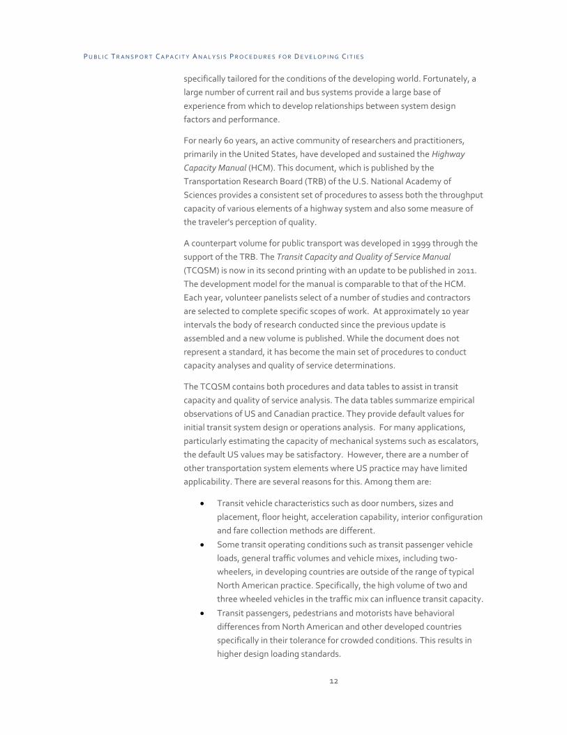
specifically tailored for the conditions of the developing world. Fortunately, a
large number of current rail and bus systems provide a large base of
experience from which to develop relationships between system design
factors and performance.
For nearly 60 years, an active community of researchers and practitioners,
primarily in the United States, have developed and sustained the Highway
Capacity Manual (HCM). This document, which is published by the
Transportation Research Board (TRB) of the U.S. National Academy of
Sciences provides a consistent set of procedures to assess both the throughput
capacity of various elements of a highway system and also some measure of
the traveler's perception of quality.
A counterpart volume for public transport was developed in 1999 through the
support of the TRB. The Transit Capacity and Quality of Service Manual
(TCQSM) is now in its second printing with an update to be published in 2011.
The development model for the manual is comparable to that of the HCM.
Each year, volunteer panelists select of a number of studies and contractors
are selected to complete specific scopes of work. At approximately 10 year
intervals the body of research conducted since the previous update is
assembled and a new volume is published. While the document does not
represent a standard, it has become the main set of procedures to conduct
capacity analyses and quality of service determinations.
The TCQSM contains both procedures and data tables to assist in transit
capacity and quality of service analysis. The data tables summarize empirical
observations of US and Canadian practice. They provide default values for
initial transit system design or operations analysis. For many applications,
particularly estimating the capacity of mechanical systems such as escalators,
the default US values may be satisfactory. However, there are a number of
other transportation system elements where US practice may have limited
applicability. There are several reasons for this. Among them are:
Transit vehicle characteristics such as door numbers, sizes and
placement, floor height, acceleration capability, interior configuration
and fare collection methods are different.
Some transit operating conditions such as transit passenger vehicle
loads, general traffic volumes and vehicle mixes, including two-
wheelers, in developing countries are outside of the range of typical
North American practice. Specifically, the high volume of two and
three wheeled vehicles in the traffic mix can influence transit capacity.
Transit passengers, pedestrians and motorists have behavioral
differences from North American and other developed countries
specifically in their tolerance for crowded conditions. This results in
higher design loading standards.

P U B L I C T R A N S P O R T C A P A C I T Y A N A L Y S I S P R O C E D U R E S F O R D E V E L O P I N G C I T I E S
13
There are some unique traffic regulatory and engineering practices
which are particular to North American practice such as right turn on
red traffic signals.
High pedestrian volumes at intersections, beyond the range of most
North American experience, can affect overall vehicle flow and
therefore transit vehicle flow.
Specific measures of the pattern of travel demand over the day (e.g.,
peaking characteristics) may vary in different countries.
More widespread use of bus rapid transit (BRT) systems in developing
countries and much more heavily used urban rail systems provides a
rich data set from which to extrapolate findings to other cities.
1.1 OBJECTIVES The objectives of this work are:
To provide a technical resource for transit planners and designers in
developing cities in their public transport capacity and performance
analysis work irrespective of mode. Specifically, to develop databases
and analytical procedures, modeled on those in the TCQSM that will
enable practitioners in the developing world to analyze existing
systems and services and/or plan new ones This volume includes
appropriate data tables and case studies of the application of selected
capacity and service quality analysis procedures using data collected
and/or appropriate to developing city conditions.
To provide a basic technical resource for academics and researchers
to use in their capacity building and research activities
As such, the document and its procedures will be incorporated into the
curricula of the World Bank’s urban transport capacity building program and
serve as a resource for the capacity building efforts of the Bank’s partners.
1.2 AUDIENCES It is expected that the primary audience for this document are public transport
planning and design practitioners, academics and researchers in developing
countries. Secondarily, it serves the same functions for academics and
researchers and to a certain extent, practitioners in the developed world.
1.3 APPLICATIONS This document is useful for both planning, design and systems analysis
purposes. The tables and procedures from this document can enable a
transportation system planner to scale each element of a rail or an enhanced
bus transportation system to the design passenger load for the system. In this
context, it is assumed that a transportation system of known required

P U B L I C T R A N S P O R T C A P A C I T Y A N A L Y S I S P R O C E D U R E S F O R D E V E L O P I N G C I T I E S
14
passenger capacity is to be planned and/or designed. The exhibits in this
manual will enable each component to be appropriately scaled to meet that
requirement. This report identifies those elements which limit overall capacity
as the traveler enters uses and departs from the transportation system. For
example, in a typical bus rapid transit or light rail system, there are a number
of “bottlenecks” (running ways/intersections, station platforms, turnstiles (if
applicable) vehicles, etc.) which can limit the overall capacity. In essence, the
overall system capacity is the minimum of the capacity of each of system
element.
Alternatively, the procedures can be used to analyze the performance of
existing transit systems and provide techniques to estimate the effects of
changes such as vehicle size, stop configuration and service patterns on the
capacity of the system and hence the quality of service offered to its
customers. This is particularly useful in planning for increased service
utilization at some time in the future. The procedures will enable the
assessment of a variety of measures to meet a target system capacity.
1.4 USING THE MANUAL This manual supplements the Transit Capacity and Quality of Service Manual
with information assembled for cities in developing countries. It is useful in
addressing two basic types of capacity analysis – one assessing the
performance of an existing transit line or system and the other in planning for
a new facility.
Assessing performance of an existing facility includes:
analyzing travel times and delay,
analyzing observed bus queues at principal stations (stops) and
congested intersections,
identifying overcrowded vehicles and stations, and
identifying car-bus-pedestrian conflicts and delays at critical locations
Assessing future conditions includes:
determining vehicle requirements for anticipated future peak
demands
providing sufficient number of vehicles to avoid overcrowding, and
designing rights-of-way and junctions (where permitted) and stations
to accommodate needed bus, rail and passenger flows.
The techniques for assessing bus rapid transit systems differ from those from a
rail system. Therefore, each is discussed separately.
The specific factors of the transit services that influence capacity included in
this work, irrespective of mode are:

P U B L I C T R A N S P O R T C A P A C I T Y A N A L Y S I S P R O C E D U R E S F O R D E V E L O P I N G C I T I E S
15
1. Running way capacity including the role of safe separation distance,
signal/control systems and junctions and turnarounds.
2. Platform capacity including allowance for circulation, waiting space,
number size and location of platform ingress/egress channels
3. Facility access elements including doorway and corridor widths,
turnstiles and other barrier gates
4. Fare collection systems including staffed fare booths and ticket
vending machines
5. Level changing systems including capacity of elevators, escalators
and stairs
6. Vehicle design elements including consist lengths, interior
configuration, doorway number, locations and widths.
7. Passenger loading standards which include the design occupancy
level for vehicles and stations.
The report has a section on facility emergency evacuation analysis in the
discussion of platform capacity to assure adequate life safety in the event of
fire or other event.
1.5 MANUAL ORGANIZATION Subsequent chapters of this guide are as follows:
Chapter 2 gives general guidelines pertaining to transit capacity and quality of
service. It contains some underlying concepts and principles.
Chapter 3 sets forth bus system capacity guidelines and estimating
procedures.
Chapter 4 contains rail rapid transit capacity guidelines
Chapter 5 contains guidance on rail and bus stations
There are a number of appendices which discuss data collection procedures
and offer some sample analyses. After the discussion for each analytical
procedure, there is a numerical problem which applies the concept to actual
practice.

P U B L I C T R A N S P O R T C A P A C I T Y A N A L Y S I S P R O C E D U R E S F O R D E V E L O P I N G C I T I E S
16
2 TRANSIT CAPACITY, QUALITY, SERVICE
AND PHYSICAL DESIGN
A good understanding of the interrelationship among capacity, resource
requirements and design in transportation operations is necessary to assess
how changes in transit design characteristics influence service quality, the
user’s perception of value of service. This section sets forth basic transit
capacity concepts, identifies the factors that influence capacity and shows how
capacity relates to quality of service and costs. It establishes the policy and
planning framework for the chapters that follow.
2.1 TRANSIT CAPACITY Transit capacity deals with the movement of both people and vehicles. It is
defined as the number of people that can be carried in a given time period
under specified operating conditions without unreasonable delay or hazard
and with reasonable certainty.1
Capacity is a technical concept that is of considerable interest to operators,
planners and service designers. There are two useful capacity concepts –
stationary capacity and flow capacity. Scheduled transit services are
characterized by customer waiting at boarding areas and traveling in discrete
vehicles along predetermined paths. The waiting area and the vehicle itself
each have a stationary capacity measured in persons per unit of area. Transit
services also have a flow capacity which is the number of passengers that can
be transported across a point of the transportation system per unit of time.
While this is usually thought of as the number of total customers per transit
line per direction per hour, flow capacity can be measured for other elements
of the system including corridors, fare turnstiles, stairs, elevators and
escalators.
2.2 KEY FACTORS INFLUENCING CAPACITY The capacity of a transit line varies along a route. Limitations may occur along
locations between stops (way capacity), at stations and terminals (station
capacity) or at critical intersections or junctions where way capacity may be
reduced (junction capacity). In most cases, station capacity is the critical
1 Source: Transit Capacity and Quality of Service Manual.

P U B L I C T R A N S P O R T C A P A C I T Y A N A L Y S I S P R O C E D U R E S F O R D E V E L O P I N G C I T I E S
17
constraint. In some stations, junctions near stations may further reduce
capacity.
The key factors which influence capacity include the following:
the type of right-of-way (interrupted flows vs. uninterrupted flows),
the number of movement channels available (lanes, tracks , loading
positions, etc.),
the minimum possible headway or time spacing between successive
transportation vehicles,
impediments to movement along the transit line such as complex
street intersections and “flat” rail junctions,
the maximum number of vehicles per transit unit (buses or rail cars),
operating practices of the transit agency pertaining to service
frequencies and passenger loading standards, and
long dwell times at busy stops resulting from concentrated passenger
boardings and alightings, on-vehicle fare collection and limited door
space on vehicles
The equations and guidelines shown in table 2.1 show how these factors can
be quantified. Further details are shown in subsequent sections.
TABLE 2-1: SUMMARY OF TRANSIT VEHICLE AND PASSENGER CAPACITY ESTIMATE
People per channel = 3600 x green x passengers x vehicles (Eq. 2.1)
Per berth per hour headway cycle vehicle unit
Minimum headway (h) = green x (dwell + dwell time + clearance time) (Eq.2.2)
cycle time variance
operating margin Source: H. Levinson
Passengers per unit depends on vehicle size and internal configuration,
passengers per unit and agency policy on the number of people per vehicle.
This policy can be approximately represented as total passengers per seat
times the number of seats. Alternatively, a better approximation would be the
passengers per meter of vehicle length times train length. An even better
approximation would be to add the number of seats to the vehicle floor area
available for standees divided by an occupancy standard of passengers per unit
of area, the latter varying by type of service, e.g., commuter rail versus
downtown people mover, commuter bus versus CBD circulator.
Service frequency is normally governed by the peak demands at the maximum
load section. Then it is necessary to assess if and how this demand can be

P U B L I C T R A N S P O R T C A P A C I T Y A N A L Y S I S P R O C E D U R E S F O R D E V E L O P I N G C I T I E S
18
accommodated at the critical constraint that governs capacity along a transit
line. The critical capacity limitations normally occur at the points of major
passenger boarding, alighting and interchange, outlying terminals, key
junctions and (for surface transit), congested intersections.
Some guidance on service design to increase capacity are enumerated below:
A simple route structure usually results in higher capacities and better
service reliability. There is less passenger confusion at stations,
impacting dwell times for both bus and rail systems and less bus-on-
bus congestion. Accordingly, especially for rail rapid transit,
branching should be avoided (or at least kept to a simple branching of
two lines)
Stop and station dwell times should be kept to a minimum by
providing off-vehicle fare collection and level entry of buses and rail
cars.
Dispersal patterns of station boardings and alightings generally
permit higher capacities than situations where passenger movements
are concentrated at a few locations.
“Crush” passenger loads should be avoided wherever possible since
they may increase station dwell times, reduce service reliability and,
in the end, reduce passenger throughput.
Various analytical methods provided bases form estimating vehicle
and passenger capacity. However, these results should be cross-
checked with actual operating experience.
Peak ridership estimate: transit capacity analysis should be based on a
peak 15 minute flow rate. This normally occurs during the morning
and evening rush hours. However, sometimes there are noon hour
and weekend peaks.
Use peak 15 minute passenger flow rather than peak hour flow rates
since ridership demand is not uniform over an entire peak period.
Fifteen minute flow rates can be obtained by direct measurement.
Commonly a peak hour factor is often used. This factor represents
the ratio of the hourly observed passenger volume to the peak 15
minute period time 4. It is a measure of the dispersion of riders about
the peak period.
The appropriate design volume for transit systems should be the peak
15 minutes since designing for the average over the peak hour will
result in operationally unstable service during peak intervals within
the peak period which have a disproportionate share of travel.
In some large urban areas, there is little variation in ridership over the
peak period. This suggests that the ridership is constrained by
capacity. Where possible, increased capacity should be provided.

P U B L I C T R A N S P O R T C A P A C I T Y A N A L Y S I S P R O C E D U R E S F O R D E V E L O P I N G C I T I E S
19
2.2.1 TH E O R E T IC A L V S . P R AC T IC AL OPE R AT I NG C AP AC I T Y
One of the most important capacity considerations is to distinguish between
maximum theoretical or crush capacity and practical operating capacity, also
called schedule design capacity). A transit vehicle may have an absolute
“maximum” capacity usually referred to as the crush load. This commonly the
capacity cited by vehicle manufacturers. The absolute capacity assumes that
all space within the vehicle is loaded uniformly at a specified passenger density
and that occupancy is uniform across all vehicles throughout the peak period, a
condition that rarely happens in practice. Similarly a rail line or a bus system
operating in an exclusive right of way may have a theoretical minimum
headway (time between two successive vehicles) based on station dwell times,
vehicle propulsion characteristics and safety margins. From these
characteristics, the theoretical maximum capacity measured as vehicles per
hour per direction can be determined. However, random variations in dwell
times, caused by such things as diminished boarding and alighting flow rates
on crowded trains, reduces the maximum or theoretical line capacity.
Operation at maximum capacity strains the system and should be avoided.
They result in serious overcrowding and poor reliability. Therefore, scheduled
design capacities should be used. This capacity metric takes into consideration
spatial and temporal variation and still results in some but not all transit
vehicles operating at crush capacity.
Further, the arriving patterns of passengers and vehicles at transit stops during
peak periods may result in some vehicles having lower than capacity loads
particularly if there is irregularity in the gap between successive arriving
vehicles. Finally, there can be a “diversity of loading” for parts of individual
vehicles (e.g., in partial low-floor LRT vehicles or buses with internal steps) and
among vehicles in multi-vehicle consists such as heavy rail trains.
Error! Reference source not found. below illustrates the relationship between
schedule and crush capacity of passengers on vehicles and scheduled track or
running way capacity. The person capacity is the product of the two, which is
represented by the areas of a rectangle between the origin and a specific
vehicle and track capacity. In both cases, the practical operating capacity is
less than the maximum capacity. The shaded area represents the likely range
of rush hour conditions.
This report recommends methods of achieving practical transit capacity during
normally encountered operating conditions. Where capacity is influenced by a
measure of dispersion of some characteristic such as stop dwell time or vehicle
headway, this is also noted. For example, line capacity is usually influenced by
both the mean and distribution of dwell times at the critical stop along the line.
At higher levels of dispersion of dwell times around the mean, capacity
diminishes in a predictable way.

P U B L I C T R A N S P O R T C A P A C I T Y A N A L Y S I S P R O C E D U R E S F O R D E V E L O P I N G C I T I E S
20
TABLE 2-2 MAXIMUM AND SCHEDULE CAPACITY
F
Crush
capacity
E
Schedule
Peak Scheduled Capacity Domain
capacity D
Ve
hic
le c
ap
aci
ty
(ve
h./
hr.
)
A B C D E F
Schedule capacity
Maximum capacity
Running way capacity (veh./hour)
The user is cautioned against designing a transit service in which the capacity
is just sufficient enough to meet expected peak passenger volumes. Transit
operations are characterized by various random events, many of which are not
in the direct control of operators particularly in bus operations. Operating at or
near capacity leaves the operator little margin to respond to such events
without substantial service disruption.
The purpose of measuring capacity is not just to provide a measure of system
capability to transport passengers but also to provide some insight into the
effect of service and physical design on customer service quality. When the
demand for a service exceeds its schedule design capacity, service quality
deteriorates either due to overcrowding on vehicles or at station platforms or
diminished ability of customers to board the next arriving transport vehicle
since it is already fully loaded, increased dwell times and hence decrease
revenue speeds. A more useful measure of service performance than capacity
from the customer perspective is the comfort level on vehicles which is usually
a function of the ratio of customers to vehicle capacity or available space per
passenger.

P U B L I C T R A N S P O R T C A P A C I T Y A N A L Y S I S P R O C E D U R E S F O R D E V E L O P I N G C I T I E S
21
2.3 QUALITY OF SERVI CE In contrast with capacity, which is largely a technical and quantitative concept,
quality of service on the other hand is a more qualitative concept. It represents
the value to the passenger of the service provided. Quality can be measured by
customer response to a number of service characteristics. In only a few cases,
however, do actions taken by transit operators (e.g., smoother
acceleration/deceleration, more gradual turning on rail systems and smoother
bus maneuvering) translate directly into a measurable change in some service
characteristic valued by customers. For example, increasing the skill of drivers
through better training does not readily convert to an improved perception of
quality. On the other hand, larger vehicle sizes and shorter waiting times at
bus or rail stops due to more frequent service directly result in measureable
changes in service attributes valued by passengers.
Two service attributes of value to customers can be influenced by the design
decisions of transportation operators. These are comfort (related to operating
and physical factors) and operating speed. Comfort is a function of the
relationship between demand (over which an operator usually has little
control) to capacity (over which an operator has considerable control). Service
speed is more than just the maximum vehicle speed. It represents the total
travel time of the passenger trip including waiting time at the boarding stop,
passenger service times at downstream stops, time lost at intersections or
decelerating and accelerating and getting into and out of stations, and time
actually in motion. The service planning and design elements of a transit
system (vehicles, stations, service frequency, operating practices etc.) will
influence both speed and comfort. This document shows through analysis of
empirical data, the relationship between service inputs and customer quality.
Service quality measurement can be portrayed as a letter level in the range of
A through F, with A representing a high quality and F a low quality. For the
attribute of passenger comfort, level of service A represents a very non-
congested condition and F, a level associated with very limited movement
within vehicles and platforms. Each of the letters represents a specific range of
densities measured in person per square meter. Owing to cultural differences
throughout the world, there are varying levels of tolerance or acceptability for
standee and seating densities. As a result, the class intervals of the densities
associated with each of the letter attributes will vary among cities throughout
the world. For passenger speed, a measure of distance per time (i.e.,
kilometers per hour) is most appropriate.
Another service attribute valued by passengers is reliability, the variation in
travel times (or speed) between trips or between days. This is a more complex
attribute than comfort and speed. Poor reliability is the result of randomness
in certain transit system operating processes. In high frequency services,

P U B L I C T R A N S P O R T C A P A C I T Y A N A L Y S I S P R O C E D U R E S F O R D E V E L O P I N G C I T I E S
22
where passengers arrive randomly at stops, the customer waiting time when
arrivals between vehicles are uniform is one-half of the headway. However,
when this uniform interval is disrupted by factors such as intersection delay, or
variability in time spent at bus stops, the average waiting time is increased.
The time variability at stops and in the case of buses – at intersections, also
results in variations in the travel times of customers already on the vehicle.
While some factors that introduce randomness are beyond the control of
transit operators, variation in time can be minimized through better service
design, scheduling practices and street operations management. Traffic signal
priority, exclusive bus lane enforcement, more efficient fare collection, better
station design and headway based scheduling are examples of such measures.
Poor reliability has consequences for both customers and operators. A service
with poor day-to-day requires riders to add buffer time to their planned
departure time to account for the probability of late arrivals of buses and trains
and variation in travel speeds. As such, a more reliable service, all other things
being equal has value to customers. Reliability also has an effect on in-vehicle
passenger comfort. Variation in the headway of scheduled vehicles results in
irregular loading patterns of vehicles and diminishes effective capacity. On
high frequency bus services, particularly where scheduled headway is nearly
the same as the traffic signal cycle length at critical intersections, there is a
tendency for buses to bunch and travel in platoons. Grade separated transit
generally has better reliability than transit vehicles subject to street traffic
interference.
While this does not diminish the theoretical capacity, it does reduce the
practical or effective capacity. This is because with headway intervals longer
than the scheduled headway, the number of customers arriving at a stop
between successive buses will exceed the design arrival rate for some of the
buses, resulting in overcrowding,
Conversely, vehicles arriving at intervals shorter than the design headway will
be underloaded. This load imbalancing deteriorates customer service quality
and operators add vehicles to compensate for this. Further, reliability has
another impact on operating costs. “Schedule recovery” time must be build
into vehicle and crew schedules so that delays do not accumulate over the
course of a peak period or day.
These result in the need for more vehicles to provide the same service
frequency and capacity. improvements in reliability also result in reductions in
“schedule recovery time” and hence on the number of vehicles/drivers and
mechanics required to carry a given number of people. For the purposes of
this report, procedures to improve reliability such as reduction of dwell time
variability, will be introduced not only so that reliability itself can be improved
but also as a means of improving comfort levels and reducing operating costs.

P U B L I C T R A N S P O R T C A P A C I T Y A N A L Y S I S P R O C E D U R E S F O R D E V E L O P I N G C I T I E S
23
The importance of service quality in transit capacity analysis cannot be
overstated. Transit operators should be mindful that the urban
transportation marketplace is mode competitive. While it might be
technically possible to design a service using a loading standard of 7 or 8
passengers per square meter, a number of customers will find that level
intolerable and will seek alternate means of travel including walking (in the
case of short distance trips), riding with someone else, riding taxis or
purchasing a motorcycle or car. Accordingly, such loading standards should
be thought of as interim measures until higher capacity at lower crowding
can be achieved.
2.4 RELATIONSHIP BETWEEN CAPACITY, QUALITY AND COST Transit production cost is rarely discussed in the context of transit capacity
since conventional thinking holds that capacity and cost are related in a linear
fashion. That is, doubling capacity requires doubling production cost. The
interrelationship is actually far more complex. A key determinant of practical
or effective capacity is variability in such things as interarrival times of
scheduled vehicles and dwell times at stops. While some of these are random
variation over which the transit operator has little control, some strategies
such as traffic signal priority and all-door loading of buses through off-board
fare collection can reduce variability and thereby positively increase capacity.
Actions to reduce variability also reduce passenger wait time, improve travel
speeds and reduce transit operating costs. The following are specific examples:
Dwell time variability results in headway variation, reduced effective
capacity due to vehicle bunching and increased customer wait time.
The reduced effective capacity (discussed in section 3.5 for buses)
results in adding more vehicles to produce the required capacity.
Dwell time and intersection time variability result in variability in
travel times between transit terminals. To assure timely departure of
the next trip to which the bus or train is assigned, additional time in
the schedule must be added. In order to maintain a specific headway,
more vehicles must be assigned to the service.

P U B L I C T R A N S P O R T C A P A C I T Y A N A L Y S I S P R O C E D U R E S F O R D E V E L O P I N G C I T I E S
24
3 BUS SYSTEM CAPACITY
3.1 INTRODUCTION Bus rapid transit (BRT) systems are increasing in importance and use in cities
throughout the developing world. They can be implemented quicker than rail
rapid transit and may cost substantially less even in total life cycle cost terms.
They can also serve as a precursor to future rail systems.
This chapter provides guidelines for estimating the capacity of BRT lines. It
overviews existing operational experience, describes the design and operating
factors that influence capacity, sets forth procedures for estimating bus
vehicles and passenger capacities and presents additional analyses related to
bus operations, service quality and capacity.
BRT, in contrast with rail rapid transit operates in a variety of environments. It
may run on segregated, fully grade separated running ways, e.g., in reserved
freeway lanes railroad rights of way, or in arterial street median busways or
single or dual curbside bus lanes. Sometimes, buses may have to operate in
mixed traffic environment. From a capacity perspective, operation through
traffic signal controlled environments is common.
3.2 OPERATING EXPERIENCE There is a growing body of information on the number of buses and people
carried by BRT lines. Examples of the peak-hour, peak direction passengers
carried by high-capacity bus systems in the developing world are shown in
Error! Reference source not found..
3.3 BUS SERVICE DESIGN ELEMENTS AND FACTORS The specific factors that influence capacity are as follows. This report treats
each of the elements of bus transit service independently and provides
empirical data on the effect of the design elements on service capacity and
quality They are:
1. Running way type and configuration including degree of segregation,
service location (curb lanes vs. median lanes), the number of lanes
(e.g., passing lanes at stations) and in the case of curb lanes, access to
the second lane for passing buses, intersection spacing, and traffic

P U B L I C T R A N S P O R T C A P A C I T Y A N A L Y S I S P R O C E D U R E S F O R D E V E L O P I N G C I T I E S
25
engineering features like signal programs (e.g., cycle length and
number of phases). The availability of space for terminal operations
also influences capacity.
2. Intersection characteristics including traffic signal cycle lengths and
phases, signal priority vehicle turning movements, near side vs. far
side vs. mid block stops.
TABLE 3-1: HOURLY PASSENGER VOLUMES OF H IGH CAPACITY BUS TRANSIT SYSTEMS IN THE DEVELOPING WORLD
Region City
Peak Volume (pphpd)*
Asia Ahmedabad 3,000
Beijing 4,100
Guanzhou 25,000
Hangzhou 6,600
Jakarta 4,000
Jinan 3,600
Seoul 6,700
Latin America Belo Horizonte 16,000
Bogota 45,000
Curitiba 14,000
Mexico City 9,000
Porto Alegre 26,100
Sao Paulo 20,000
Quito 8,000
Africa Lagos 10,000
*pphpd – passengers per hour per direction
1. Fare collection system elements including location of fare payment,
(on-board vs. off-board) complexity of fare structure and fare media
employed (cash, cards etc.)
2. Bus design factors including vehicle length, seating configuration,
floor height, door numbers and width, location and size
characteristics
3. Bus boarding area factors such as bus stop length and width, number
of berths, approach to assignment of multiple routes to boarding
berths, availability of passing lanes and platform height in relation to
floor height.

P U B L I C T R A N S P O R T C A P A C I T Y A N A L Y S I S P R O C E D U R E S F O R D E V E L O P I N G C I T I E S
26
4. Service design factors including service frequency, route structure,
operation of multiple routes or branches on a corridor and serving
stations, vehicle platooning and station spacing
5. Policy factors such as enforcement of parking restrictions at stops
and along the running way, encouragement of multi-door boarding
and alighting and passenger loading standards.
These elements are discussed separately and the effect of changes on service
quality and capacity is augmented with empirical tables. Essentially, the
capacity of a route in passengers per period per direction is a product of the
running way capacity (vehicles per hour per direction) and the vehicle capacity
(passengers per vehicle). Error! Reference source not found. illustrates how
the design decisions affect the components of system capacity.
TABLE 3-2: TRANSIT DESIGN ELEMENTS AND THEIR EFFECT ON CAPACITY
Running Way Capacity
Time at Stops
Time at Intersections
Time Moving
Vehicle Capacity
Vehicle Characteristics
Vehicle size (length) X
Seating configuration/Aisle width
X X
Floor height, number of internal steps
X X
Door location and size X
Acceleration./Deceleration rates
Stop Characteristics
Platform height X
Number of loading berths X
Platform size X
Berth assignment to routes X
Number of entry/exit channels
X
Fare Collection Characteristics
On board/off board X
Fare media X
Fare structure complexity X
Running Way Characteristics
Speed limit X
Stop spacing X

P U B L I C T R A N S P O R T C A P A C I T Y A N A L Y S I S P R O C E D U R E S F O R D E V E L O P I N G C I T I E S
27
Passing capability X
Pedestrian behavior X
Other policies
Lane enforcement X
Loading standard X
Traffic law enforcement
Intersection characteristics
Traffic signal cycle times and splits
X
Phases X
Turn restrictions X
Pedestrian flows and behavior
X
3.4 OVERVIEW OF PROCEDURES Error! Reference source not found. and Error! Reference source not found.
illustrate procedures for assessing the capacity of existing and proposed BRT
lines respectively. These tables also show ways of increasing vehicle capacity.
TABLE 3-3: CAPACITY ASSESSMENT OF EXISTING BRT L INE
Data Collection – Critical Stop 1. For each major stop determine the mean dwell time and dwell time standard headway standard deviation. 2. Identify the critical stop. This is the one with the maximum of the mean dwell time plus two standard deviations. 3. Determine the peak period passenger boarding and alighting rate and magnitude at the critical stop.
4. Determine the probability (failure rate) of a bus entering the critical station without a stopping place available to board passengers.
Data Collection – Critical Intersection
1. Determine pedestrian crossing volume per peak period that conflicts with right turning vehicles in the bus lane. (curb lane only)
2. Determine right turning vehicle movements from bus lane (curb lane only) during the same period 3. Identify the green time for turns and traffic signal cycle time. 4. Identify if there are major bus-auto or bus-pedestrian conflicts
Data Analysis 1. Determine the capacity at the critical bus stop. (Section x.x) 2. Determine capacity at critical intersection. (Section x.x)
Estimate Future Volumes 1. Estimate future passengers 2. Establish bus frequency 3. Determine conflicting right hand turns
Capacity Expansion Estimate 1. Determine if capacity expansion is necessary over the planning horizon 2. Determine required capacity expansion by year
P U B L I C T R A N S P O R T C A P A C I T Y A N A L Y S I S P R O C E D U R E S F O R D E V E L O P I N G C I T I E S
28
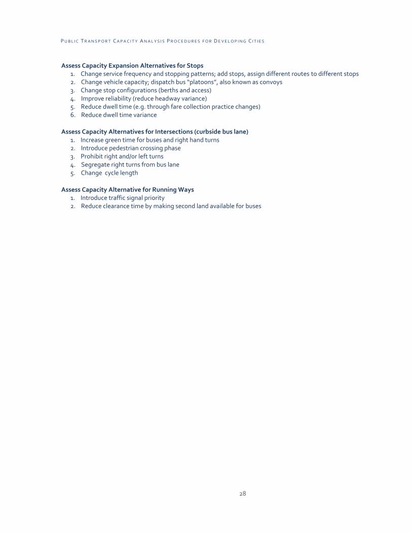
Assess Capacity Expansion Alternatives for Stops 1. Change service frequency and stopping patterns; add stops, assign different routes to different stops 2. Change vehicle capacity; dispatch bus “platoons”, also known as convoys 3. Change stop configurations (berths and access) 4. Improve reliability (reduce headway variance) 5. Reduce dwell time (e.g. through fare collection practice changes) 6. Reduce dwell time variance
Assess Capacity Alternatives for Intersections (curbside bus lane) 1. Increase green time for buses and right hand turns 2. Introduce pedestrian crossing phase 3. Prohibit right and/or left turns 4. Segregate right turns from bus lane 5. Change cycle length
Assess Capacity Alternative for Running Ways 1. Introduce traffic signal priority 2. Reduce clearance time by making second land available for buses

P U B L I C T R A N S P O R T C A P A C I T Y A N A L Y S I S P R O C E D U R E S F O R D E V E L O P I N G C I T I E S
29
TABLE 3-4: CAPACITY ASSESSMENT OF A PROPOSED BRT L INE
Develop a Proposed Running Way
1. Degree of separation between buses and cars
2. Develop passing opportunities at stops
3. Determine traffic signal controls at stops and major intersections
4. Determine spacing and location of passenger boarding stops
Initiate a Proposed Service Design
1. Develop service frequency
2. Identify trip patterns
3. Propose vehicle size and type
4. Propose fare collection system (on board, off board)
5. Develop a passenger loading standard
Data Collection – Critical Stop
1. Estimate expected passenger loading per time period at each stop.
2. Estimate on-board load after bus leaves each stop.
3. Estimate expected dwell time and dwell time variance at each stop
4. Identify the critical stop for planning purposes.
5. From the initial estimate of bus frequency, determine the probability.
(failure rate) of a bus entering the critical station without a place available to board
Passengers
Data Collection – Critical Intersection
1. Determine pedestrian crossing volume per peak period which conflicts with
right turning vehicles in the proposed bus lane. (curb lane only)
2. Determine right turning vehicle movements from bus lane (curb lane only)
3. Identify the green time for right hand turns and cycle time.
Data Analysis
1. Determine the capacity at the critical bus stop. (Section x.x)
2. Determine capacity at critical intersection. (Section x.x)
Estimate Future Volumes
1. Passengers
2. Bus frequency
3. Conflicting right hand turns
Assess Adequacy of initial Plan
1. Determine if passenger flow at critical stop can be maintained
2. Determine if vehicle flow through critical intersection can be maintained.
Assess Capacity Expansion Alternatives for Stops
1. Change service frequency
2. Change vehicle capacity
3. Change stop configurations (berths and access)
4. Improve anticipated reliability (reduce headway variance)
5. Reduce anticipated dwell time

P U B L I C T R A N S P O R T C A P A C I T Y A N A L Y S I S P R O C E D U R E S F O R D E V E L O P I N G C I T I E S
30
6. Reduce anticipated dwell time variance
Assess Capacity Alternatives for Intersections (curbside bus lane)
1. Increase green time for buses and right hand turns
2. Introduce pedestrian crossing phase
3. Prohibit right turns
4. Segregate right turns from bus lane
Assess Capacity Alternative for Running Ways
1. Introduce traffic signal priority
2. Reduce clearance time by making second land available for buses
Both sets of procedures underscore the need to reduce the number of and
dwell time at stops.
3.5 OPERATI ON AT BUS STOPS Computing the capacity of a bus route operating in an exclusive right of way is
conceptually straightforward. It is essentially the product of the number of
vehicles which can be processed through a critical point on the route and the
number of passenger spaces of each vehicle during the peak period of
passenger demand.
Where the buses operate under uninterrupted (ideal) flow conditions, as along
grade separated busways or on freeways, the capacity per station or stop is
essentially 3,600 seconds divided by the time spent per stop multiplied by the
number of effective loading positions (berths). When buses stop at signalized
intersections, less time is available for bus movement. In both cases, the stop
processing time includes the waiting time to reach a vacant berth, the dwell
time needed to board and discharge passengers, the clearance time between
successive vehicles and time to re-enter the traffic stream as needed. In some
cases, conflicts between right turning traffic and pedestrians may limit the
capacity of the curb lanes.
The delay in waiting for a vacant berth is a function of dwell time distribution,
number of berths at the stop and whether or not buses have the ability to
overtake other buses at stops to access vacant loading berths.
Boarding/discharging dwell time is a function of vehicle, passenger demand
and fare collection methods. Clearance time depends on the availability of the
adjacent lane (exclusively for buses or not) and the traffic volume and
dispersion of traffic gaps on the adjacent lane.
The distribution of dwell times at the critical stop2 in a transit system can limit
the number of vehicles per hour that can pass through the station.
Accordingly, measures that reduce the dwell time or dwell time variation can
2 The critical stop is the one in which the mean plus two standard deviations of the dwell time is
maximum.

P U B L I C T R A N S P O R T C A P A C I T Y A N A L Y S I S P R O C E D U R E S F O R D E V E L O P I N G C I T I E S
31
improve system capacity and the quality of service to customers. The
individual factors that govern bus operations at stops are described below
followed by a discussion of incorporating these factors together to estimate
stop capacity.
An operating margin must be introduced in estimating station capacity. This is
a buffer time to allow for random variation in dwell time. An operating margin
allows for dwell time variability without disrupting scheduled operating.
Another design attribute must be accounted for in berth or stop calculations is
the “failure rate.” This is defined as the percentage of the time that a bus or
train will approach a stop and not find a berth available. This is a particularly
important concept for on-street bus and tram operations with stops on the far
side of intersections. If the failure rate is too high, transit vehicles will tend to
“spill back” through the respective intersection, causing undue congestion for
vehicle flows in the perpendicular direction. This has been an issue for a
number of busway applications in China (Kunming, Shijiazhuang).
3.5.1 BE R T H (ST O P ) C AP AC IT Y UN DE R S IM P LE C O ND IT IO NS
3.5 .1 .1 L O A D I N G B E R T H D Y N A M I C S A N D C A P A C I T Y
For this discussion, it is assumed that there is a single route serving the bus
stop so that passengers can select any arriving bus to travel to their
destination and further there is a single boarding location at the bus stop.
Given the variation in arrival rates of buses and the dwell (service) times of
buses, there is a possibility that an arriving bus will not be able to immediately
access the stop. If the arrival and service time distributions are know with any
precision, the probability of delay due to bus berths being occupied, referred
to as the failure rate, can be computed. Transit planners can reduce this rate
by reducing the mean or variability of the service time, increasing the headway
or reducing the headway variance. Alternatively, the number of bus berths can
be increased.
The operating margin (tm) is defined as:
tm = s Z = cv td Z (Eq. 3.3)
Where,
tm = operating margin (sec)
s = standard deviation of dwell times
Z = the standard normal variable corresponding to a specific failure rate (one-
tailed test)
cv = coefficient of variation (standard deviation/mean) of dwell time; and

P U B L I C T R A N S P O R T C A P A C I T Y A N A L Y S I S P R O C E D U R E S F O R D E V E L O P I N G C I T I E S
32
td = average dwell time (sec).
The table below shows the z-statistic value associated with certain failure
rates.
TABLE 3-5: Z-STATISTIC ASSOCIATED WITH STOP FAILURE RATES
Acceptable Failure Rate
Z -statistic
1% 2.326
5% 1.645
10% 1.282
There is a tradeoff between the failure rate and the berth capacity. A high
operating margin is required to assure that the failure rate is tolerable. One
method is to specify a failure rate and through actual observation of mean and
standard deviation of dwell time, estimate the capacity of the stop. At
reasonable failure rates, this value represents the practical sustainable
capacity. The maximum theoretical capacity will occur at a failure rate which
may be unacceptably high.
3.5 .1 . 2 B E R T H C A P A C I T Y W I T H U N I N T E R R U P T E D F L O W
The capacity of a bus berth in vehicles per hour can be estimated by the
following equation:
B = 3600/(td + tm + tc) (Eq. 3.1)
Where,
B = berth capacity in buses per hour
td = mean stop dwell time
tm = operating margin
tc = clearance time, (the time for stopped buses to clear the station, minimum
separation between buses, and time to re-enter the traffic stream
3.5 .1 . 3 C A P A C I T Y F O R S T O P S NE A R S I G N A L I Z E D I N T E R S E C T I O N S
The maximum flow capacity at a bus stop near a signalized intersection in
vehicles per hour is:
Bl = 3600(g/C)/(td(g/C) + tm + tc) (Eq. 3.2)
Where,
Bl = buses per berth per hour
g = green time at stop

P U B L I C T R A N S P O R T C A P A C I T Y A N A L Y S I S P R O C E D U R E S F O R D E V E L O P I N G C I T I E S
33
C = cycle time at stop
td = mean stop dwell time
tc = clearance time, the time to re-enter the traffic streams defined above
tm = operating margin
The capacity of a bus stop in buses per hour is shown in Error! Reference
source not found. below. This table shows values for average dwell times
from between 10 and 80 seconds and a range of coefficient of variation
between .3 and .6. In all cases, a maximum allowable failure rate of 5% was
assumed. These estimates should be adjusted downward for flow interrupted
by traffic control devices by the ratio g/C
TABLE 3-6: BUS BERTH CAPACITY (UNINTERRUPTED FLOW) FOR A STATION WITH A S INGLE BERTH
Dwell Time Coefficient of Variation
Dwell Time Mean (sec.)
0.3 0.6
10 144 120
20 90 72
30 65 51
40 51 40
50 42 32
60 36 27
70 31 24
80 27 21
90 24 19
Table entries are in buses per berth hour Source: Transit Capacity and Quality of Service Manual
Actual US experience shows considerable scatter in observed coefficients of
variation. TCRP Report 263 indicates that the coefficients decreases as the
overall dwell time increases. Coefficients between 40% and 60% were
representative of dwell times of 20 seconds or more but tend to underestimate
variability when mean dwell times are lower.
An issue arises when the critical bus stop requires more than one loading berth
to meet the capacity requirement. If buses are able to pass each other, then
the capacity of the stop, measured in vehicles per hour, will increase almost
linearly with the number of berths. However, if the bus stop does not permit
3 St. Jacques, K.R. and Levinson, H. S. TCRP Report 26, Operational Analysis of Bus Lanes on
Arterials, TRB, national Research Council, Washington, DC 1997.

P U B L I C T R A N S P O R T C A P A C I T Y A N A L Y S I S P R O C E D U R E S F O R D E V E L O P I N G C I T I E S
34
buses to pass each other, then the efficiency of successive berths beyond the
first will be diminished. That is, doubling the number of berths will not double
the effective capacity. Simulation studies, augmented by empirical data found
the following relationships (Error! Reference source not found.) between the
number of berths and the capacity of the multi-berth stop.
Some cities, especially in South America, provide bypass lanes around stations
on median arterial busways. The service pattern should be analyzed. The
capacities should be computed for the busiest stop for each group of buses.
For example, if stop A can accommodate 80 buses per hour and stop B can
accommodate 100 buses per hour, the system capacity would be the sum
assuming that different buses serve each stop.
TABLE 3-7: ACTUAL EFFECTIVENESS OF BUS BERTHS
On-Line Station Off-Line Station
Number of Berths
Effectiveness of Berth
Total Effectiveness* of
all Berths
Effectiveness of Berth
Total Effectiveness* of
all Berths
1 1.0 1.00 1.00 1.00
2 .75 1.75 .85 1.85
3 .70 2.45 .80 2.65
4 .20 2.65 .65 3.25
5 .10 2.75 .50 3.75
*Ratio of the capacity of the number of berths to a single berth. (Source: Research Results Digest 38, Operational Analysis of Bus lanes on Arterials, Transportation Research Board.
Using observed data from Barcelona, Spain, Estrada et al., (2011) determined
that the incremental capacity of a second loading berth was a function of the
standard deviation of dwell time and developed the chart below to assess this
value.

P U B L I C T R A N S P O R T C A P A C I T Y A N A L Y S I S P R O C E D U R E S F O R D E V E L O P I N G C I T I E S
35
FIGURE 3-1INCREMENTAL CAPACITY OF A SECOND BUS BERTH:
Source: Estrada et al., (2011)
Example: A transit route at the critical stop has a mean dwell time of 30 seconds with a coefficient of variation of 0.3. Compute the capacity of the system in vehicles per hour if 3 bus bays are provided. Note that there are no passing lanes at the bus stop. Capacity of single stop berth = 87 Effectiveness of first three berths (on-line) = 2.45 Capacity of 3 bus berths (on line) = 87 * 2.45 =213 buses per hour
3.6 BUS BERTH CAPACITY IN MORE COM PLEX SERVICE
CONFI GURATIONS The US transit capacity manual has procedures for determining the increase in
capacity with successive berths at a bus stop. The operating system for this
analysis assumes that each arriving bus accesses the first vacant berth and that
buses can board and discharge customers at any berth. In cases where the stop
serves multiple routes, passengers must observe the location of arriving buses
in order to board the proper vehicle.
In several circumstances outside of the US, the service operating system is
quite different. Transmilenio in Bogota is a case in point. The Transmilenio
running way consists of two lanes in each direction and buses are able to pass
each other in most circumstances. Most of the stops are served by several
routes. The routes are partitioned into route groups and the group is assigned
to a single berth. A plan view of a typical station is shown in Error! Reference
source not found. below. Note that some stations have two or three such
modules.

P U B L I C T R A N S P O R T C A P A C I T Y A N A L Y S I S P R O C E D U R E S F O R D E V E L O P I N G C I T I E S
36
FIGURE 3-2: PLAN V IEW OF TRANSMILENIO BUS STATION
In the figure berth 2 has a queuing space behind it in the boarding lane.
Boarding and discharging is not done in the queuing space. The queuing space
can be accessed from the bypass lane. The set of routes assigned to berth 1 is
distinct from the routes assigned to berth 2.
In order to present a set of tools to analyze this and other situations, a set of
simulation models was developed to determine the capacity of the following
four configurations:
Single loading berth – no queuing space
Single loading berth – queuing space for one bus
Dual loading berth – no queuing space
Dual loading berth – queuing space for one bus
Capacity was defined for several acceptable failure rates including (5%, 10%
and 25%) with the failure rate being defined as the probability that an arriving
bus will not be able to enter either a vacant berth or a queuing space. Other
variables in each of these assessments included mean service time with values
of 20, 20, 40, 50, 60 and 75 seconds4. The final two input variables were service
time variability and arrival rate variability. To simplify the assessment, these
two variables were staged as either high or low. Definitions are shown in the
table below.
TABLE 3-8: SERVICE VARIABILITY LEVELS
Input Level Definition
Service time variability Low CV* = 0.4 times mean service time
High CV = 0.8 time mean service time
Headway variability Low CV = 0.4 times mean headway
High CV = 0.8 time mean headway
* Coefficient of variation = standard deviation/mean
4 The term service time is used in these calculations. Service time includes the dwell time (time the
bus is stopped) as well as the safe separation time between successive vehicles – about 12 seconds.

P U B L I C T R A N S P O R T C A P A C I T Y A N A L Y S I S P R O C E D U R E S F O R D E V E L O P I N G C I T I E S
37
This analysis resulted in the development of 8 tables – two for each of the four
service domains described above and the presence or absence of a traffic
signal at the station. These are shown in tables 3-22 through 3-29. A summary
table appears in Error! Reference source not found. These tables require
relatively little data collection effort to estimate station capacity. On high
volume BRT services, mean service times can be obtained with about an hour’s
worth of observations. A similar length of time would enable a determination
of low or high values of service time and headway variability. These data are
for articulated (18m) buses. Non-articulated (13 m) buses are likely to increase
capacity slightly since the time for the bus to clear the station is about 5
seconds less. Conversely, a bi-articulated bus takes 7-8 seconds to clear the
station.
The determination of an acceptable failure rate is more complex. In cases
where some buses bypass certain stops, the inability of buses serving the stop
to access either the berth or the queuing area may result in blocking through
buses. In such cases a low failure rate of about 10% is suggested. In high
volume cases, a high failure rate may result in a queue which may not dissipate
for a long time, perhaps as much as several minutes. The photograph (Error!
Reference source not found.) below shows a long queue at a TM stop.
Fortunately, this dissipated within 2 minutes.
TABLE 3-9: TRANSMILENIO STATION (BOGOTA) W ITH LONG QUEUE

P U B L I C T R A N S P O R T C A P A C I T Y A N A L Y S I S P R O C E D U R E S F O R D E V E L O P I N G C I T I E S
38
TABLE 3-10: BUS BERTH CAPACITY (UNINTERRUPTED FLOW) FOR A STATION WITH A SINGLE BERTH
Mean Service Time (sec.)
Case Berths Queue Space
Traffic Signal* 30 40 50 60 75
1 1 Yes Yes 60 45 35 25 25
2 1 Yes No 60 50 40 25 25
3 1 No Yes 35 30 25 20 15
4 1 No No 45 40 30 20 15
5 2 Yes Yes 80 55 40 40 35
6 2 Yes No 80 65 50 45 35
7 2 No Yes 60 50 40 30 25
8 2 No No 80 65 50 35 30
Table entries are capacities in vehicles per hour with a failure rate of 10% with moderate service time variation and moderate headway variation. In this table, dwell time includes time to enter the stop, and time to depart the stop. This is about 15 seconds.
* If yes, green to cycle time ratio is 0.5
3.7 STOP DWELL T IMES AND PASSENGER BOARDING T IMES The procedures described above require using the mean and distribution of
stop dwell times as inputs to determine bus berth capacity. The common
method of estimating stop dwell time is through observation of the passenger
flow at the critical door multiplied by the boarding or alighting time per
passenger. The boarding and alighting rates per passenger are a function of
variables such as method of fare payment, bus floor height relative to platform
height and level of crowding already on the bus. These can be determined
through actual observation.
Error! Reference source not found. below illustrates a range of reported
observations of transaction time per passenger for bus systems. These entries
assume a single boarding and alighting stream per doorway.
TABLE 3-11: PASSENGER SERVICE T IMES (SEC./PASS.)
Situation Observed Range
Suggested Default
Boarding
Pre-payment* 2.2-2.8 2.5
Single ticket or token 3.4-3.6 3.5
Exact change 3.6-4.3 4.0
Swipe or dip card 4.2 4.2
Smart card 3.0-3.7 3.5

P U B L I C T R A N S P O R T C A P A C I T Y A N A L Y S I S P R O C E D U R E S F O R D E V E L O P I N G C I T I E S
39
Alighting
Front door 2.6-3.7 3.3
Rear door 1.4-2.7 2.1
* includes no fare, bus pass, free transfer, pay on exit and off-board payment rear door boarding.
Add 0.5 sec./pass to boarding times when standees are present.
Subtract 0.5 sec./pass from boarding times and 1.0 sec./pass. from front-door alighting times on low floor
buses.
Source: Transit Capacity and Quality of Service Manual
The stop dwell time is also influenced by customer discipline and operating
practices. With on-board driver-controlled fare collection, boarding customers
enter through the front door and ideally exit through the rear door. In practice,
however, several passengers exit through the front door. This delays boarding
passengers and sometimes extends dwell times. The critical door capacity
calculation must take this into account.
Off board or conductor-controlled fare collection allows for multiple door
boarding and alighting and can reduce stop dwell times.
The common method for estimating dwell time requires as an input the
expected value and distribution of number of boarding passengers at each
stop. This is captured in the following equation:
td = Pata + Pbtb + toc (Eq. 3.4)
where:
td = average dwell time;
Pa = alighting passengers per bus through the busiest door (p);
ta = alighting passenger service time (pass./sec.);
Pb = boarding passengers per bus through the busiest door (p);
tb = boarding passenger service time (pass./sec.); and
toc = door opening and closing time.
Example: At a busy bus stop with off-board fare collection, the design number of boardings is 12 and the
design number of alightings is 14. There are two single stream doors, and customers use each equally for
boardings and alighting. Assume door opening and closing time is 2 seconds. Compute the expected
dwell time for this stop.
td = Pata + Pbtb + toc
= (6 * 3.3) + (7 * 3.3)+ 2 = 45 seconds

P U B L I C T R A N S P O R T C A P A C I T Y A N A L Y S I S P R O C E D U R E S F O R D E V E L O P I N G C I T I E S
40
Fernandez et al (2007) proposed a formulation for dwell times using data from
TranSantiago. Two models were calibrated – one for BRT trunk buses and the
other for feeder buses. On the BRT buses passenger fares were collected
through contactless smart cards through the front door. The feeder fares were
collected through conventional fare technology.
For the BRT routes, the model was of the form:
td = 9.32 + max j=door((2.05 + .88d1)Bj + (3.32 – 1.93d2)Aj
where,
td = dwell time
d1 = dummy variable = 1 if boardings > 40, 0 otherwise
Bj = boardings through door j
d2 = dummy variable = 1 if alightings > 15, 0 otherwise
Aj = alightings through door j
Loosely interpreted, there is a 9.3 second time for door opening and closing.
For each boarding customer, the time is 2.05 seconds unless the boardings at
the stop exceed 40. Similarly the discharge rate is 3.32 seconds per customer
unless the discharge rate exceeds 15, in which case the rate reduces by 1.93
second per customer. For the feeder routes, the model was
td = 8.04 + max j=door((3.82 + .88d1)Bj + (3.32 – 1.93d2)Aj
where,
d1 = dummy variable = 1 if boardings <5, 0 otherwise
d2 = dummy variable = 1 if alightings > 25, 0 otherwise
These models have reasonably good explanatory power with the R2 (the
proportion of variation in dwell times explained by the model) being 0.84 and
0.72 for the trunk and feeder buses respectively. Additional research in this
area is warranted, particularly in determining the effect of crowded buses on
dwell time.
Predictive models of dwell time which use boarding and alighting data have
limited utility in the planning and design of new services since travel demand
forecasting models do not explain boardings and alightings by individual trip.
Further, in high capacity bus rapid transit systems, the mean dwell time is
more a function of the physical design of station and vehicle elements such as
doorway width, fare collection scheme and the difference in height between
the bus floor and the boarding platform. Some limited data on dwell time of
the high capacity bus rapid transit service in Bogota, Colombia is shown in

P U B L I C T R A N S P O R T C A P A C I T Y A N A L Y S I S P R O C E D U R E S F O R D E V E L O P I N G C I T I E S
41
Error! Reference source not found. below. The Transmilenio system has high
floor buses, level loading platforms at stations, off-board fare collection and
articulated buses with three loading doors each capable of accommodating
two parallel boarding streams. This mode of operation was designed
specifically to minimize mean dwell time.
TABLE 3-12: STOP DWELL T IME – BOGOTA TRANSMILENIO
Stop Time Period
Mean (sec.)
Standard Deviation
(sec.)
Coefficient of Variation
Calle 100 AM Peak 24 17 0.71
PM Peak 22 14 0.64
Calle 72 AM Peak 19 15 0.79
PM Peak 20 10 0.50
Source: Transmilenio, SA
3.8 CLEARANCE T IME Clearance time must be considered when buses need to re-enter traffic stream
from curb-side stop. Clearance time has three components. (1) the time for a
bus to leave the berth, (2) the time needed before the next bus arrives and (3)
the time separation needed to re-enter the traffic stream. US experience has
found that total clearance times are roughly 15 to 20 seconds. The first two
components require about 10 seconds. The third component is necessary
when buses must change lanes. The amount of re-entry time ranges up to 15
seconds depending on the hourly traffic volumes in the adjacent lane. (See
Error! Reference source not found.)
With curbside lanes and high bus traffic volumes, passing a bus in one of the
bus berths is necessary. This is more likely to happen where there are a
number of routes assigned to the bus lane. In some instances, (Madison
Avenue, New York City) the second lane from the curb is a bus lane that
reduces the re-entry time. In cases where the adjacent lane is not exclusive,
the re-entry time can be estimated from the table below. Yield to bus laws can
reduce this re-entry time.
The exit time is estimated at 5 seconds for a 13 meter bus and about 10 seconds for an articulated bus.
This clearance time (exit plus re-entry time) should be added to the dwell time to compute the total time
associated with boarding and discharging passengers at the stop.

P U B L I C T R A N S P O R T C A P A C I T Y A N A L Y S I S P R O C E D U R E S F O R D E V E L O P I N G C I T I E S
42
TABLE 3-13: RE-ENTRY T IME
Adjacent Lane Volume (veh/hr)
Average Re-entry
Delay (sec)
100 1
200 2
300 3
400 4
500 5
600 6
700 8
800 10
900 12
1000 15
Source: Transit Capacity and Quality of Service Manual
3.9 CALCULATION PROCEDURE Bus stop capacity calculations are straightforward. The formula below shows
the effect of boarding time and clearance time and the effective capacity of
multiple berth bus stops. Essentially the computation procedure is to find the
product of the effective number of loading areas and the capacity per loading
area. The formula is generalized for a near side bus stop at a signalized
intersection. For a midblock, far side or unsignalized intersection where the
bus lane is in the major travel direction, g/C would be equal to one.
Bs = NelBl =Nel * (3600*(g/C))/(tc + td(g/C) +Zcvtd) (Eq. 3.5)
Where,
Bs = bus stop capacity (bus/h)
Bl = individual loading area bus capacity (bus/h)
Nel = number of effective loading areas
3,600 = seconds per hour
g/C = green time ratio (effective green time to total signal cycle
time)
tc = clearance time (s)
td = mean dwell time (s)
Z = standard normal variable corresponding to a desired failure
rate (one-tailed test)

P U B L I C T R A N S P O R T C A P A C I T Y A N A L Y S I S P R O C E D U R E S F O R D E V E L O P I N G C I T I E S
43
cv = coefficient of variation of dwell times
Example: Compute the capacity of a bus stop with two in-line berths where the average dwell time is 40 seconds with a coefficient of variation of 0.3 and the g/C ratio is 0.5. Assume 500 cars per hour in the adjacent lane and the tolerable failure rate is 5%.
Bs = NelBl =Nel (3600*(g/C))/(tc + td(g/C) +Zcvtd)
Nel =1.75 g/C = 0.5 tc = 5 seconds (from table x) plus 10 seconds equal 15 seconds td = 40 seconds cv = 0.3 Z = 1.645 (one-tailed z-statistic associated with 5% failure rate)
Bs = 1.75* ((3600 * .5)/(15 +(40 * 0.5)+ (1.645*0.3*40))=46 buses per hour
3.10 VEHICLE PLATOONI NG The methods of capacity analysis in the previous sections assume there is a
single route operating within the BRT corridor and the service design includes
constant service intervals within time periods. There are conditions where a
different operating pattern is in place and alternate methods of capacity
analysis should be considered for vehicle platooning and multiple routes in the
corridor.
Vehicle platooning (operation of “virtual bus trains”) is an operating system in
which two vehicles move in tandem along a busway. These can be either on
the same route or different routes. The advantage of such a scheme is
increased capacity where capacity is constrained by stop dwell time and stops
have multiple loading berths. Platooning can also reduce the probability of
bunching because the headway to provide the same capacity is longer and
irregular vehicle arrivals are a lower proportion of the total arrival interval.
Platooning can also fa-cilitate signal priority because the number of priority
events will be reduced. Finally, platooning can also obviate the need for a
passing lane at BRT stops.
If there are two routes in the two bus platoon, the operating scheme may be
either a constant sequence (i.e. Route A is always the first bus in the platoon.)
or random sequence. If both routes start at a common terminal, the constant
sequence is more easily attained. The benefit of constant sequencing is that
customers can wait at specific locations on the loading platform since the bus
for their destination will consistently arrive at that location. With random
sequencing, customers have to reposition themselves when buses arrive
causing dwell times to increase and reducing capacity. Through the use of
intelligent transportation system technology, the sequence can be made
known ahead of time. However, some passenger confusion will remain even if
such measures are implemented.

P U B L I C T R A N S P O R T C A P A C I T Y A N A L Y S I S P R O C E D U R E S F O R D E V E L O P I N G C I T I E S
44
At signalized intersections, it may be difficult to maintain the platoon without
some ITS application such as traffic signal priority or use of “count down”
clocks to ensure that the entire platoon can proceed through a green phase.
For the purpose of capacity analysis the following analytical technique is
offered.
This is an extension of the generalized capacity equation for vehicles at stops.
The number of effective loading areas for platooned operation (Nel) is
estimated to be 1.85 for two-bus platoons.
Bs = NelBl = Nel3,600(g/C)/(tc + td(g/C)+Zcvtd) (Eq. 3.6)
Where,
Bs = Bus stop capacity (buses/hour)
Bl = Individual loading area bus capacity
Nel = Number of effective loading areas = 1.85 for platooned arrival
of two buses
3,600 = seconds per hour
g/C = green time ratio (ratio of effective green time to cycle time.
This equals 1.0 for unsignalized intersections)
tc = clearance time (sec.)
td = mean dwell time (sec.) (This is the dwell time associated with
the route with the highest number of passenger transactions in cases where
the platoon serves two routes.)
Z = standard normal variable corresponding to desired failure rate (one
tail) ; and
cv = coefficient of variation of dwell time
Example: Compare the capacity in vehicles per hour of a two berth bus stop with platooning and non-platooing of arriving buses if the dwell time mean is 30 seconds and the standard deviation is 10 seconds. Assume a 5% permitted failure rate, a non-signalized intersection and a 10 second clearance time. Platooned arrival: Note: cv = standard deviation/mean Therefore, cvtd = standard deviation
Bs = NelBl = Nel 3,600(g/C)/(tc + td(g/C)+Zcvtd) =(1.85 * 3600)/(20 + 30 (1) + (1.645 * 10)) = 100 buses per hour
Non platooned arrival (no passing): Bs = NelBl = Nel 3,600(g/C)/(tc + td(g/C)+Zcvtd) =(1.75 * 3600)/(20 + 30 (1) + (1.645 * 10)) = 95 buses per hour

P U B L I C T R A N S P O R T C A P A C I T Y A N A L Y S I S P R O C E D U R E S F O R D E V E L O P I N G C I T I E S
45
Table 3.11 provides some typical values of bus capacity at a stop with multiple
berths. In the table the assumed failure rate is 5% and the clearance time is 10
seconds.
TABLE 3-14: STOP CAPACITY FOR MULTIPLE BERTH STOPS AT VARIOUS DWELL T IME LEVELS
Bus Berths
Dwell Time (sec.)
Coefficient of Variation of Dwell Time
1 2 3 4 5
20 0.3 93 162 204 255 278
20 0.6 76 132 166 208 227
30 0.3 68 118 149 186 203
30 0.6 54 95 119 149 163
40 0.3 53 93 117 146 160
40 0.6 42 74 93 116 127
Table entries are in buses per hour
Source: Calculations based on Transit Capacity and Quality of Service Manual
3.11 VEHICLE CAPACITY There is considerable diversity in the size, capacity and configuration of transit
buses among cities in the developing world. Only full size buses suitable for
bus rapid transit (BRT) services are considered here. Error! Reference source
not found. below shows a range of typical bus sizes in Pakistan.
TABLE 3-15: TYPICAL BUS MODELS IN PAKISTAN
Manufacturer Model Floor Height
Length (m)
Seating Capacity
Standing* Capacity
Ashok Leyland 222 High 10.9 50 20
Articulated bus High 16 52 20
Volvo 8700 Low 12 40 N/A
8700 Low 13.5 45 N/A
8700 Low 15 53 N/A
8700 High 12 53 N/A
8700 High 13.5 55 N/A
Tata STAR ULF Ultra low
12 27 35
STAR LF Low 12 44 35
* Manufacturer’s estimate
A generally applicable approach to the estimation of bus capacity is:
Vehicle Capacity = # seats + area available for standing/area per
standee (set as a standard)

P U B L I C T R A N S P O R T C A P A C I T Y A N A L Y S I S P R O C E D U R E S F O R D E V E L O P I N G C I T I E S
46
For planning purposes, the standee density standard would be the amount of
space each standee would be assigned to allow an acceptable level of
crowding across an average peak hour. For “crush” design purposes, the
density would correspond to the peak fifteen minutes. In either case, this is a
policy standard that reflects social norms and available resources. It also
reflects the type of service provided and the nature of the market. The longer
that people must stand (e.g., for on long distance CBD-oriented commuter
services), the more space generally assigned to each standing passenger
Typical standards for urban bus and rail services are shown in Error!
Reference source not found. below.
TABLE 3-16: URBAN BUS AND RAIL LOADING STANDARDS
Place of Application Typical Number of
Standees per Square
Meter
EU 4-5
US, Canada 3-4
Latin America BRT 6-8
Asia 8-10
A generalized formula for the capacity of a bus given its geometry, door and
seating configuration and acceptable loading standard is as follows:
Vc = (L -1)*(W-0.2) –(0.5DnWsDw) + (1- Sa/Ssp)N((L-1)-Dn(Dw+2Sh)
Ssp Sw
Where,
Vc = Total vehicle capacity (seats plus standees)
L = Vehicle length (m)
W = Vehicle width (m)
Dn = Number of doorways
Ws= Doorway setback (m)
Dw = Doorway width (m)
Sa = Area of single seat (m2) [0.5 m
2 for transverse,0.4 m
2 for
longitudinal]
Ssp = Standing space per passenger

P U B L I C T R A N S P O R T C A P A C I T Y A N A L Y S I S P R O C E D U R E S F O R D E V E L O P I N G C I T I E S
47
N = Vehicle arrangement
[2 for 2 seats/row, 3 for 2 + 1 seats/row, 4 for 2 + 2 seats/row, 5 for 2 + 3
seats/row]
Sw = Seat pitch [0.69 m for transverse, 0.43 m for longitudinal]
Sb = Single set-back allowance (additional space for storing open
door) [0.2 m]
Error! Reference source not found. below shows typical capacities for a range
of bus types (single unit, articulated and bi-articulated) and loading standard.
In each case, the assumed number of doors is 2 for single unit, 3 for articulated
and 4 for bi-articulated buses. The first table is for transverse seating, while the
second is for longitudinal (peripheral) seating.
TABLE 3-17: BUS VEHICLE CAPACITY
Transverse Seating
Bus type single articulated bi-articulated
Doorways 2 3 4
Length (m) 13 20 25
Standees/sq. m.
4 80 126 160
5 87 137 174
6 94 148 188
7 101 158 203
8 109 169 217
Longitudinal Seating Bus type single articulated bi-articulated
Doorways 2 3 4
Length (m) 13 20 25
Standees/sq. m.
4 86 136 172
5 97 153 194
6 108 170 217
7 120 188 239
8 131 205 262
The passenger capacity of a bus depends on its seating configuration and the
allowable loading design standard. The use of low-floor buses complicates the
analysis since in low floor buses, vehicle wheel wells and internal stairs reduce
passenger capacity.

P U B L I C T R A N S P O R T C A P A C I T Y A N A L Y S I S P R O C E D U R E S F O R D E V E L O P I N G C I T I E S
48
As in other discussions about capacity, these estimates are maximum
theoretical capacity which should be adjusted downward to allow for variation
in demand through the peak hour, diversity of loading within vehicles and non-
uniformity of the headway.
3.12 PASSENGER CAPACI TY OF A BUS L INE The passenger capacity of a bus route can be estimated by multiplying the bus
(vehicle) capacity at the busiest stop by the scheduled design capacity of the
vehicle used. Results should be compared with actual data for a similar route in
the same city.
Thus, if 90 articulated buses per hour are accommodated at the busiest
boarding point, and the schedule design capacity is 100 passengers, the line
could carry about 9,000 passengers per hour. Since many BRT lines have
passing opportunities at stations (or there are dual bus lanes), this capacity
would be doubled for dual berths. Note that busy BRT lines in cities carry
20,000 people per hour in the peak direction of travel. The line capacity
calculation is illustrated below:
C = VNelBl =VNel * (3600*(g/C))/(tc + td(g/C) +Zcvtd) (Eq. 3.8)
Where,
C = line capacity in passengers per hour
V = vehicle scheduled capacity
Bl = individual loading area bus capacity (bus/h)
Nel = number of effective loading areas at critical stop
3,600 = seconds per hour
g/C = green time ratio (effective green time to total signal cycle
time)
tc = clearance time (s)
td = mean dwell time (s)
Z = standard normal variable corresponding to a desired failure
rate (one-tailed test)
cv = coefficient of variation of dwell times

P U B L I C T R A N S P O R T C A P A C I T Y A N A L Y S I S P R O C E D U R E S F O R D E V E L O P I N G C I T I E S
49
Example: Compute the line capacity of a bus line with three in-line berths at the critical stop where the average dwell time is 200 seconds with a coefficient of variation of 0.3 and the critical g/C ratio is 0.6. Assume a 10 second clearance time and the tolerable failure rate is 5%.
Bs = VNelBl =Nel (3600*(g/C))/(tc + td(g/C) +Zcvtd) V = 80 passengers
Nel =2.45 (from table 3.x) g/C = 0.5 tc = 10 seconds td = 20 seconds cv = 0.3 Z = 1.645 (one-tailed z-statistic associated with 5% failure rate)
C = 80* 2.45* ((3600 * .6)/(10 +(20 * 0.5)+ (1.645*0.3*20))=14,100 passengers per hour
3.13 TRANSIT OPERATIONS AT INTERSECTI ONS While the throughput capacity of a bus transit route is usually limited by the
operation at the critical stop, the capacity can also be constrained by traffic
operations at critical intersections. This may happen in cases where there is
considerable intersection interference from other vehicles making left or right
turns, pedestrians and bicyclists, low green to cycle time ratios in the direction
of bus travel, or where the bus service operates on the minor approach of an
intersection. On curbside bus lanes, the traffic conflict occurs when right
turning cars and trucks occupy the bus lane, and are impeded by crossing
pedestrians in the direction of travel of the bus. In median bus lanes, there is
generally no comparable conflict since normal design practice is to have signal
controlled left turns in a distinct lane from the exclusive bus lane. Transit
intersection capacity is also influenced by the location of any bus stops at the
intersection.
3.13.1 CUR B LA NE O PE R AT IO N
Traffic conflicts at signalized intersections can impede bus movements when
the green per cycle time is limited and/or when right turns from or across the
bus lane conflict with through buses. The delay can constrain bus capacity
where right turn volume conflicts with heavy pedestrian movements. The
result is reduced capacity in the curb or interior bus lane.
3.1 3. 1. 1 S C R E E N I N G F O R R I G H T TU R N C O N F L I C T S
The impact of pedestrian-right turn conflicts on curb bus lane capacity may call
for restricting the right turns, or possibly grade separating the conflicting
pedestrian movement. A simple method to assess these effects is set forth in
TCRP Report 90 Bus Rapid Transit Implementation Guidelines. A more
detailed method is available in the Transit Capacity and Quality of Service
Manual at page 4-48.

P U B L I C T R A N S P O R T C A P A C I T Y A N A L Y S I S P R O C E D U R E S F O R D E V E L O P I N G C I T I E S
50
The simplified method assumes each pedestrian channel takes a specified time
to cross the area in which there is a conflict with right turns; in effect, each
pedestrian delays each right turn by this time. The time lost can be estimated
by weighing the time per pedestrian by the number of pedestrians and right
turns per signal cycle. The green time which is lost due to pedestrian-right turn
conflicts can then be approximated by the following equation:
Δt = rpts/L (Eq. 3.9)
Where,
Δt = green time to be gained per cycle,
r = right turns/cycle (peak 15 minutes)
p = conflicting pedestrians/ cycle (peak 15 minutes)
ts = time per pedestrian (e.g. 3 or 4 seconds), and
L = number of pedestrian channels in crosswalk (e.g., 1 to 4)
The lost time per cycle is deducted from the green time per cycle. If the
remaining effective green time is less than 25% of the cycle time, then the turn
conflicts will not impede operation of the curbside bus lane.
Estimated lost time per signal cycle by conflicting right turns and pedestrian
volumes is shown in Table 3.13.
TABLE 3-18: LOST T IME PER CYCLE DUE TO R IGHT TURN-PEDESTRIAN CONFLICTS
Time Lost per Cycle at 3 Seconds per Pedestrian
Typical Values of R/Nc * P/Nc
1 Lane 2 Lanes 3 lanes 4 Lanes
4 12 6 4 3
8 24 12 8 6
12 36 18 12 9
16 48 24 16 12
20 60 30 20 15
24 72* 36 24 18 R = right turns per hour
Nc = number of cycles per hour
P = pedestrians per hour
Source: Levinson, TCRP Report 90, 2003
For a 60 second cycle, time loss should not exceed 25% of the cycle time or 15
seconds. In the table, the boldface values are not acceptable, and turns should
be prohibited.

P U B L I C T R A N S P O R T C A P A C I T Y A N A L Y S I S P R O C E D U R E S F O R D E V E L O P I N G C I T I E S
51
Example: A curbside bus lane operates at an intersection where the green time per cycle is 50
seconds and the cycle time is 90 seconds. The number of pedestrian crossings per hour 200 and the
number of right turning cars is 120 per hour. Is there sufficient time to operate a curbside lane with
right turning vehicles in the bus lane?
The number of pedestrian crossing per cycle is 5(200/40). The number of right tuning vehicles per
cycle is 3 (120/40). The number of conflicts per cycle is 20. If there are 3 pedestrian lanes and the time
per pedestrian in one channel is 3 seconds then the time lost due to conflicts is 20 (5 * 4 *3/3). The
percentage loss per cycle is 20/90 or 22%. This is less than the 25% threshold, suggesting that the
right turn movement volume is compatible with the curbside bus lane.
3.1 3. 1. 2 A D J U S T M E N T F O R M I X E D TR A F F I C I N T H E R I G H T L A N E
The previous procedure provided guidance as to whether the volume of right
turn movements would affect capacity of the bus lane. The actual reduction in
capacity can be computed by applying a mixed traffic adjustment factor to the
estimated lane capacity.
Mixed Traffic Adjustment Factor
where,
fm = mixed traffic adjustment factor (from Error! Reference source
not found.)
fl = bus stop location factor (See table below)
v = curb lane volume (veh/h)
c = curb lane capacity (veh/h) (see table below)
The curb lane capacity is a function of the number of conflicting pedestrians
and the traffic signal g/c ratio and is shown in Error! Reference source not
found.
TABLE 3-19: BUS STOP LOCATION CORRECTION FACTOR
Bus Stop Location Factors
Bus Stop Location Type 1 Type 2 Type 3
Near side 1 0.9 0
Mid block 0.9 0.7 0
Far side 0.8 0.5 0
Type 1 – Buses have no use of adjacent lane Type 2 – Buses have partial use of adjacent lane Type 3 – Buses have full use of adjacent lane (i.e. second lane is a
bus lane)

P U B L I C T R A N S P O R T C A P A C I T Y A N A L Y S I S P R O C E D U R E S F O R D E V E L O P I N G C I T I E S
52
TABLE 3-20: R IGHT TURN CURB LANE VEHICLE CAPACITIES
g/C Ratio for Bus Lane
Conflicting Pedestrian
Volume (ped/h)
0.35 0.4 0.45 0.5 0.55 0.6
0 510 580 650 730 800 870
100 440 510 580 650 730 800
200 360 440 510 580 650 730
400 220 290 360 440 510 580
600 70 150 220 290 360 440
800 0 0 70 150 220 290
1000 0 0 0 0 70 150
Source: Transit Capacity and Quality of Service Manual
3.14 COMPUTING BUS FACILITY CAPACITY The bus facility capacity is:
where,
B = Bus facility capacity (bus/h)
Bl = Bus loading area capacity
Nel = number of effective loading areas
fm = mixed traffic adjustment factor
3.15 MEDIAN LANE OPERATION Median arterial bus lanes are used along wide streets in many cities to avoid
the uncertainties and turbulence of curb lane operation. In the design of
median bus lanes or busways, the normal practice is to provide an exclusive
left turn lane for non-transit vehicles that is independent of the bus lane.
These lanes, provided only at signal controlled intersections normally have a
protected signal phase. The typical phasing is:
1. Busway plus through traffic on the street parallel to the busway
2. Left turns from the street parallel to the busway
3. Cross street traffic
Buses are not permitted to cross the intersection when left turns or cross
traffic have green indications.

P U B L I C T R A N S P O R T C A P A C I T Y A N A L Y S I S P R O C E D U R E S F O R D E V E L O P I N G C I T I E S
53
3.16 CAPACITY AND QUALITY REDUCTION DUE TO HEADWAY
IRREGULARITY
3.16.1 CAP AC IT Y RE DUC T IO N
Most traditional methods of transit capacity analysis with the short bus
headways common in developing cities, assume that transit vehicles arrive at a
uniform headway and decisions on the appropriate frequency are merely a
matter of assuring that the capacity offered is sufficient to carry passengers
traveling through the maximum load point constrained by a vehicle loading
standard. Over a specified time interval, this will assure that all customers will
be carried, although it may not mean that all customers may board the next
arriving bus or train.
In actuality, owing to variation in passenger arrival patterns, boarding rates
and travel time through signalized intersections there is likely to be some
variation in the vehicle interarrival time. This introduces some diminution of
actual capacity which may be quantified. If a bus is delayed enroute at the stop
just before the maximum load segment, the actual headway interval will
exceed the design or published interval. In this case, there will be more
customer arrivals than expected. This will result in either loading above the
design limit of the vehicle or some customers having to wait until the next
arriving vehicle. On the other hand, if the actual time gap is less than the
published headway, the vehicle will depart from the station with fewer
customers than the vehicle capacity. Since capacity is perishable, once the
vehicle departs the critical stop less than fully loaded, the available capacity is
lost forever. A possible strategy of holding buses at stations until the actual
headway meets the published headway results in fewer vehicles per hour
being offered which also diminishes capacity.
The method of quantification of this requires the introduction of a term called
effective frequency. This is the equivalent frequency that provides the same
capacity as a frequency with a specific variability. The effective frequency is:
fe = f/(1 + cvh) (Eq. 3.10)
Where,
fe = effective frequency (buses/hr.)
f = scheduled frequency (buses/hr.)
cvh = coefficient of variation of headway (headway standard
deviation/mean headway)
The actual capacity of the route is the product of the vehicle capacity and the
effective frequency. While this is a good framework, there is limited data
available on the factors causing headway irregularity. Evidence indicates that

P U B L I C T R A N S P O R T C A P A C I T Y A N A L Y S I S P R O C E D U R E S F O R D E V E L O P I N G C I T I E S
54
headway variability is low at terminals and increases along the route. The
appropriate method of determining actual system capacity is to review
headway coefficient of variation at the maximum load segment to determine
effective frequency.
Data from the BRT system in Jinan, China which has an exclusive median right
of way, suggest that the coefficient of variation in headway on BRT routes is
high as shown in Error! Reference source not found. below. High frequency
routes in Jinan are very susceptible to headway variation since some traffic
signal cycle times are on the order of 4 minutes, which exceeds the scheduled
headway.
TABLE 3-21: BRT HEADWAY VARIATION - J INAN, CHINA
Line number 1 2 3
Headway (min) 3 3.5 4.5
Headway cv 0.36 0.54 0.42 Source: Huang (2010)
Data from Transmilenio in Bogota, Colombia also reveal a high coefficient of
variation of headway on the order of .9 to 1.0. More precisely, this is the cv of
buses from multiple routes arriving at a major bus station and using a common
berth. The fact that there are several bus routes serving the station adds to the
headway variability.
Example: The published frequency of a BRT route is 15 vehicles per hour and the loaded vehicle capacity is 60. What is the effective capacity if the arrival rate of passengers is uniform and if the coefficient of variation of headway is about 0.3?
fe = f/(1 + cvh) = 15/(1.3) = 11.5 vehicles per hour * 60 passengers/vehicle = 690 passengers
3.16.2 EXT E NDE D WA IT T IM E DUE T O HE A DW AY IR R E G UL AR IT Y
Note that in addition to capacity reduction, headway variation also
deteriorates the quality of the customer experience by increasing the average
waiting time for buses (or trains). If headways are constant the average
waiting time is h/2 where h is the headway. It can be shown that if there is
some variation in the headway denoted by cvh, the coefficient of variation
(standard deviation /mean) of headway, the average wait time is:
w = (h/2)* (1 + cvh) (Eq. 3.11)
where,

P U B L I C T R A N S P O R T C A P A C I T Y A N A L Y S I S P R O C E D U R E S F O R D E V E L O P I N G C I T I E S
55
w = average customer wait time
h = average headway
cvh = coefficient of variation of headway (headway standard
deviation/mean headway)
There is limited understanding of how the operating environment affects
headway variation. The evidence suggests that measures such as traffic signal
priority at intersections and management of passenger loading can assist in
this effort.5
Just as in the case of capacity diminution, the headway variability causes
irregular gaps in service and more customers arrive at the stop during longer
gaps.
Example: Compute the average customer wait time at a stop if the headway is 4 minutes with no variance? What is the average wait time if the headway coefficient of variation is 0.3? Average waiting time with no variance = h/2 = 4/2 = 2 minutes Average waiting time with headway coefficient of variation of 0.3 = (h/2)* (1 + cvh)= 2 * (1.3) = 2.6 minutes
3.16.3 TR AV E L T I M E S AN D FLE E T RE QU IR E M E NT S
Proper scheduled running times are essential for proper transit operation.
Running times that exceed what is required to maintain schedules result in
higher than necessary operating costs. Excessively tight (lower than optimal)
running times, on the other hand, result in late arrivals at timepoints. If there is
not sufficient schedule recovery time built into driver schedules, inadequate
times can also cause delays in terminal departures on subsequent trips, a key
factor in late arrivals on successive stops. This requires balancing the
requirements for operating efficiency and requirement for sufficient layover
time for schedule recovery and operator breaks.
The BRT running time between terminals will depend on both the length of the
trip and the speed of travel time. The speed or travel time rate depends on the
distance between stops, the time spent at each stop and the number of buses
operating during the design period.
Normally, when bus flows are less than about 50-70 percent of the maximum
line capacity, there is little reduction in operating speeds. Beyond that point,
5 For example, on loaded buses the flow rate of customers onto vehicles is very low. Rather than
wait until all customers are on board, a policy of loading only until the flow rate falls below some
minimum value will probably increase capacity due to reduction of dwell time and dwell time
variability, each of which also influence throughput capacity on a route.

P U B L I C T R A N S P O R T C A P A C I T Y A N A L Y S I S P R O C E D U R E S F O R D E V E L O P I N G C I T I E S
56
however, there is a rapid drop in speeds to about half the free-flowing speed
when the ratio is 0.9 or more. An illustrative example for the Avenue Caracas
corridor in Bogota is shown in figure 3.3.
FIGURE 3-3: SPEED VS. FREQUENCY
0
5
10
15
20
25
30
0 20 40 60 80 100 120 140 160
Bus Frequency (buses/hr.)
Co
mm
erc
ail s
pe
ed
(k
m./h
r.)
Source: Steer, Davies, Gleave
The actual running time for each individual trip can be prepared based on
either observed or archival data. However, preparing schedules in which the
scheduled travel times varies very often throughout the day results in irregular
headways if the number of vehicles assigned is held constant or irregular fleet
assignment patterns if headways are held constant. In actual practice, the
number of time intervals must reflect a balance between accuracy in reflecting
significant predictable variation among trips and portraying a schedule which
is easy to understand by customers and avoids complicated vehicle and
staffing patterns.
The optimal half-cycle time, the scheduled time to travel between terminals
and time allowance prior to departure of the next trip, balances schedule
efficiency, operator layover and schedule recovery. Consider the extreme case
in which there is no variability in terminal to terminal time. In such case, a
sufficient time would be allowed at the end of the bus trip to allow for operator
break. Roughly 10% is allocated to this. On the other hand, for a trip with
considerable variability between days, the objective would be to provide
sufficient time to assure on-time departure on the next trip from the same
terminal. From a simple statistical test, the running time required to assure

P U B L I C T R A N S P O R T C A P A C I T Y A N A L Y S I S P R O C E D U R E S F O R D E V E L O P I N G C I T I E S
57
that the probability that there is sufficient time for 90%, 95% or 99% of trips
departing on time can be computed. Specifically, a one-tailed normal test can
be used to make this estimate. The best half cycle time would be the larger of
(1) the times necessary for driver layover and (2) the time necessary for
punctual terminal departure on the subsequent trip. A value of 95% is
appropriate. In plain terms, sufficient time should be allowed to assure that the
probability that the next trip can depart on time is at least 95%.
Mathematically, the appropriate half cycle time is:
tc = max (tm*(1+rd)), tm * (1 + (cv * z)) (Eq. 3.12)
where,
tc = half cycle time
tm = mean terminal to terminal time
rd = driver recovery percent
cv = coefficient of variation of terminal to terminal time
Z = value of unit normal z statistic corresponding to desired probability of on-
time departure for the subsequent trip. (Error! Reference source not found.)
TABLE 3-22: Z-STATISTIC FOR ONE-TAILED TEST
Desired On-time Probability for next
departure
Z -statistic
99% 2.330
95% 1.645
90% 1.280
Example: The average terminal to terminal time in the morning peak hour is 32 minutes, with a standard deviation of 0.1 minutes. Compute the half cycle time required to assure both sufficient driver break time (10%) and schedule recovery if the desired probability of on-time departure for the following trip is 95%. What would the half cycle time be if the coefficient of variation is 0.3 and the desired on time departure was 99%.
tm = 32 min. rd = 10% cv = 0.1 z95% = 1.645 z99% = 2.33 Running time for driver recovery = 1.1 * 32 = 35 minutes Running time for on-time departure = 32 * (1+(.1 *1.645)) = 37 minutes The greater of these is 37 minutes The half cycle time if the desired on-time departure rate for the next trip is 99% is: 32 * (1 + (.1 * 2.33)) =39.5 minutes

P U B L I C T R A N S P O R T C A P A C I T Y A N A L Y S I S P R O C E D U R E S F O R D E V E L O P I N G C I T I E S
58
3.17 TERMINAL CAPACITY
Some cities in developing countries have major off-street bus terminals. In
South America, cities such as Bogota and Curitiba, “integration terminals” are
an integral part of the overall system. These terminals have several important
advantages. (1) They provide a place for passengers to transfer between bus
routes (2) When located near areas of high transit demand, they remove
passenger interchanges from street stops and stations (3) They provide
sufficient capacity to serve large numbers of passengers both during rush
hours and throughout the day. (4). They can serve as stations for express
services.Thus they can permit higher roadway vehicles and passenger volumes
than with total reliance on busway operation.The berth capacity of a terminal
will depend on operating practices – both in terms of berth assignment to
routes and stop dwell times. Typical productivity in New York’s 200 berth
midtown terminal is 4 buses per berth per hour. San Francisco’s 40-berth
Transbay Terminal serves about 7 buses per berth per hour.
TABLE 3-23: APPROXIMATE CAPACITY OF S INGLE BERTH, WITH QUEUING AREA
1 Failure Rate
Service Time (sec.) Service Time CV* Headway CV
5% 10% 25%
30 40% 40% 48 58 68
40% 80% 19 33 60
80% 40% 44 49 58
80% 80% 17 37 55
40 40% 40% 43 46 54
40% 80% 23 30 49
80% 40% 32 41 46
80% 80% 17 27 40
50 40% 40% 33 35 45
40% 80% 18 22 41
80% 40% 25 28 37
80% 80% 15 19 33
60 40% 40% 25 30 37
40% 80% 15 20 37
80% 40% 23 26 33
80% 80% 13 22 28
75 40% 40% 18 25 29
40% 80% 13 18 28
80% 40% 20 22 28

P U B L I C T R A N S P O R T C A P A C I T Y A N A L Y S I S P R O C E D U R E S F O R D E V E L O P I N G C I T I E S
59
80% 80% 11 14 21
* CV – coefficient of variation = standard deviation/mean
TABLE 3-24: APPROXIMATE CAPACITY OF S INGLE BERTH, WITH QUEUING AREA
2 Failure Rate
Service Time (sec.)
Service Time CV*
Headway CV 5% 10% 25%
30 40% 40% 58 64 83
40% 80% 33 47 66
80% 40% 45 55 68
80% 80% 31 38 56
40 40% 40% 44 47 57
40% 80% 23 35 54
80% 40% 35 42 52
80% 80% 24 30 44
50 40% 40% 35 44 50
40% 80% 20 29 43
80% 40% 28 30 41
80% 80% 15 19 37
60 40% 40% 27 33 40
40% 80% 16 26 37
80% 40% 25 27 33
80% 80% 13 22 31
75 40% 40% 25 26 32
40% 80% 15 18 28
80% 40% 22 23 28
80% 80% 11 19 26
* CV – coefficient of variation = standard deviation/mean
TABLE 3-25: APPROXIMATE CAPACITY OF S INGLE BERTH, WITHOUT QUEUING AREA
3 Failure Rate
Service Time (sec.)
Service Time CV*
Headway CV 5% 10% 25%
30 40% 40% 26 37 51
40% 80% 10 12 34
80% 40% 22 34 48
80% 80% 7 9 32
40 40% 40% 23 32 44
40% 80% 6 10 23
80% 40% 18 25 38
80% 80% 7 26

P U B L I C T R A N S P O R T C A P A C I T Y A N A L Y S I S P R O C E D U R E S F O R D E V E L O P I N G C I T I E S
60
50 40% 40% 19 26 35
40% 80% 5 8 18
80% 40% 16 21 34
80% 80% 6 10 21
60 40% 40% 16 20 30
40% 80% 5 7 16
80% 40% 14 20 26
80% 80% 6 12 16
75 40% 40% 13 17 25
40% 80% 5 6 13
80% 40% 11 15 23
80% 80% 5 13
* CV – coefficient of variation = standard deviation/mean
TABLE 3-26: APPROXIMATE CAPACITY OF S INGLE BERTH, WITHOUT QUEUING AREA
4 Failure Rate
Service Time (sec.)
Service Time CV*
Headway CV 5% 10% 25%
30 40% 40% 29 47 68
40% 80% 10 12 33
80% 40% 27 40 60
80% 80%
40 40% 40% 26 37 53
40% 80% 9 10 30
80% 40% 21 27 50
80% 80%
50 40% 40% 22 30 41
40% 80% 7 9 22
80% 40% 19 25 35
80% 80%
60 40% 40% 18 23 39
40% 80% 6 8 16
80% 40% 14 21 32
80% 80%
75 40% 40% 13 18 29
40% 80% 4 6 13
80% 40% 11 16 24
80% 80%
* CV – coefficient of variation = standard deviation/mean

P U B L I C T R A N S P O R T C A P A C I T Y A N A L Y S I S P R O C E D U R E S F O R D E V E L O P I N G C I T I E S
61
TABLE 3-27: APPROXIMATE CAPACITY OF DOUBLE BERTH, WITH QUEUING AREA
5 Failure Rate
Service Time (sec.)
Service Time CV*
Headway CV 5% 10% 25%
30 40% 40% 67 75 96
40% 80% 50 68 79
80% 40% 55 58 76
80% 80% 46 55 76
40 40% 40% 50 61 76
40% 80% 43 51 66
80% 40% 42 48 60
80% 80% 32 45 59
50 40% 40% 43 48 60
40% 80% 35 47 58
80% 40% 32 37 50
80% 80% 27 35 52
60 40% 40% 37 43 52
40% 80% 27 40 49
80% 40% 25 31 43
80% 80% 23 28 41
75 40% 40% 30 33 39
40% 80% 22 29 36
80% 40% 24 28 34
80% 80% 20 25 35
* CV – coefficient of variation = standard deviation/mean
TABLE 3-28: APPROXIMATE CAPACITY OF DOUBLE BERTH, W ITH QUEUING AREA
6 Failure Rate
Service Time (sec.)
Service Time CV
Headway CV 5% 10% 25%
30 40% 40% 74 90 105
40% 80% 56 80 94
80% 40% 56 63 84
80% 80% 54 64 82
40 40% 40% 55 67 78
40% 80% 48 62 76
80% 40% 46 51 61
80% 80% 39 44 66
50 40% 40% 48 51 68
40% 80% 36 46 60

P U B L I C T R A N S P O R T C A P A C I T Y A N A L Y S I S P R O C E D U R E S F O R D E V E L O P I N G C I T I E S
62
80% 40% 37 41 52
80% 80% 32 35 50
60 40% 40% 41 45 52
40% 80% 35 42 54
80% 40% 25 33 43
80% 80% 26 32 42
75 40% 40% 30 33 41
40% 80% 27 31 45
80% 40% 24 27 34
80% 80% 20 26 36
* CV – coefficient of variation = standard deviation/mean
TABLE 3-29: APPROXIMATE CAPACITY OF DOUBLE BERTH, W ITHOUT QUEUING AREA
7 Failure Rate
Service Time (sec.)
Service Time CV*
Headway CV 5% 10% 25%
30 40% 40% 50 64 85
40% 80% 28 45 73
80% 40% 44 55 74
80% 80% 21 36 65
40 40% 40% 46 50 68
40% 80% 20 41 62
80% 40% 32 42 53
80% 80% 18 30 52
50 40% 40% 35 41 55
40% 80% 15 29 51
80% 40% 30 37 47
80% 80% 16 25 45
60 40% 40% 31 37 49
40% 80% 15 28 42
80% 40% 24 27 40
80% 80% 13 24 32
75 40% 40% 25 30 38
40% 80% 13 23 36
80% 40% 20 23 31
80% 80% 13 19 31
* CV – coefficient of variation = standard deviation/mean

P U B L I C T R A N S P O R T C A P A C I T Y A N A L Y S I S P R O C E D U R E S F O R D E V E L O P I N G C I T I E S
63
TABLE 3-30: APPROXIMATE CAPACITY OF DOUBLE BERTH, WITHOUT QUEUING AREA
8 Failure Rate
Service Time (sec.)
Service Time CV*
Headway CV 5% 10% 25%
30 40% 40% 64 79 104
40% 80% 33 49 88
80% 40% 51 59 82
80% 80% 28 44 77
40 40% 40% 50 57 81
40% 80% 23 42 65
80% 40% 38 48 60
80% 80% 24 33 55
50 40% 40% 39 50 63
40% 80% 16 37 56
80% 40% 32 37 49
80% 80% 16 25 47
60 40% 40% 31 40 54
40% 80% 15 31 47
80% 40% 25 33 42
80% 80% 13 24 32
75 40% 40% 26 31 42
40% 80% 13 23 37
80% 40% 20 26 34
80% 80% 13 20 31
* CV – coefficient of variation = standard deviation/mean

P U B L I C T R A N S P O R T C A P A C I T Y A N A L Y S I S P R O C E D U R E S F O R D E V E L O P I N G C I T I E S
64
4 RAIL CAPACITY
4.1 INTRODUCTION Rail rapid transit systems provide important public transportation service in
very large cities in developing countries. Trains operate along rights-of-way
that are completely separated from street traffic interference. They carry
large numbers of people safely and reliably. Train control signal systems
govern train operations and capacities.
This chapter provides guidance for computing the capacities of rail lines and
stations. It overviews existing operational experience, identifies the key
design and operating factors and sets forth procedures for estimating
capacities in terms of trains per track per hour, passengers per track per hour
and station platforms and access to them.
4.2 OPERATING EXPERIENCE Most rail rapid transit systems throughout the world schedule 25 to 30 trains
per hour track per hour (2 to 2.5 minute headways). A few systems, however,
operate at shorter intervals. They are found in Sao Paulo and Mexico City as
well in Hong Kong and Paris. These systems operate single lines without any
branching.
Most rail rapid transit systems throughout the world schedule 25 to 30 trains
per hour track per hour (2 to 2.5 minute headways). A few systems, however,
operate at shorter intervals. They are found in Sao Paulo and Mexico City as
well in Hong Kong, Tokyo, Moscow and Paris. These systems operate single
lines without any branching.
Some reported peak rush hour passenger volumes are given in Error!
Reference source not found.. The highest volumes, from 60,000 to over
80,000 passengers per track per hour, are found on lines in Sao Paulo and
Hong Kong.
4.3 DESIGN CONSIDERATIONS
Rail transit capacity concepts are similar to those in bus transit in several
respects. Essentially, the running way capacity of a system measured in
vehicles per hour is constrained by the occupancy of the critical station along a
route – the one with the highest combination of mean and standard

P U B L I C T R A N S P O R T C A P A C I T Y A N A L Y S I S P R O C E D U R E S F O R D E V E L O P I N G C I T I E S
65
deviation6. While there are no on-street intersections in grade separated rail
systems, other operational and design features such as terminals and junctions
also limit capacity. Further, with generally larger volumes and either elevated
or subterranean operation, level changing devices and platforms have a larger
influence on system capacity than they do in bus systems.
TABLE 4-1: HOURLY PASSENGER VOLUME OF RAIL TRANSIT SYSTEMS IN THE DEVELOPING WORLD
Region City Peak Volume (pphpd) *
Asia
Bangkok 50,000
Chongqing (monorail) 17,000
Hong Kong 50,000
Manila 26,000
Latin America
Buenos Aires 20,000
Mexico City 39,300
Santiago 36,000
Sao Paulo 60,000
*pphpd - passengers per hour per direction
Listed below are the various aspects of transit capacity that are subsequently
discussed.
1. Running way capacity including the role of safe separation distance,
signal/control systems and turnarounds.
2. Platform capacity including allowance for circulation, waiting space,
number size and location of platform ingress/egress channels
3. Facility access elements including doorway and corridor widths,
turnstiles and other barrier gates
4. Fare collection systems including staffed fare booths and ticket
vending machines
5. Level changing systems including capacity of elevators, escalators
and stairs
6 Transit analysts generally consider the critical station to be the one with the highest mean dwell
time plus two standard deviations of dwell time.

P U B L I C T R A N S P O R T C A P A C I T Y A N A L Y S I S P R O C E D U R E S F O R D E V E L O P I N G C I T I E S
66
6. Vehicle design elements including consist lengths and configuration
(discrete vehicles or open-vestibule for entire train), interior
configuration, doorway number, locations and widths.
4.4 OVERVIEW OF PROCEDURES Error! Reference source not found. and 4.3 illustrate procedures for assessing
the capacity of existing and proposed rail transit lines respectively. These
tables also show ways of increasing system capacity.
TABLE 4-2: GENERAL CAPACITY ANALYSIS PROCEDURES - EXISTING RAIL LINE
Data Collection – Critical Stop
1. For each stop determine the mean dwell time and dwell time standard deviation during
peak hour. Also determine the peak headway and headway standard deviation.
Also determine the number of on-board passengers as each train departs.
2. Identify the critical stop. This is the one with the maximum of the mean dwell time
plus two standard deviations.
3. Determine the peak period passenger boarding rate at the critical stop. Data Collection – Terminal Stop
1. Determine headway, headway variability, dwell time and dwell time variability at terminal stops. Data Analysis
1. Determine the capacity at the critical station.
2. Determine capacity at the critical terminal stop. Estimate Future Volumes
1. Passengers Capacity Expansion Estimate
1. Determine if capacity expansion is necessary over the planning horizon
2. Determine required capacity expansion by year Assess Capacity Expansion Alternatives for Stops
1. Change service frequency
2. Change vehicle capacity – change consist length
3. Improve reliability (reduce headway variance)
4. Reduce dwell time
5. Reduce dwell time variance Assess Capacity Alternatives for Terminals
1. Change operating practices – driver takes subsequent train from terminal
2. Reduce dwell time or dwell time variance
3. Add terminal platform(s)

P U B L I C T R A N S P O R T C A P A C I T Y A N A L Y S I S P R O C E D U R E S F O R D E V E L O P I N G C I T I E S
67
TABLE 4-3: CAPACITY ASSESSMENT PROCEDURE OF PROPOSED RAIL L INE
Initiate a Proposed Service Design
1. Service frequency
2. Train consist length and vehicle configuration
3. Platform sizes
4. Terminal stop configuration
5. Fare collection system
6. Level change system at stations
7. Terminal operating practices
Data Collection – Critical Stop
1. Estimate expected passenger loading per time period at each station.
2. Estimate on-board load after train leaves each station.
3. Estimate expected dwell time and dwell time variance at each station
4. Identify the critical station for planning purposes.
This is the one with the maximum of the mean dwell time plus two standard deviations. Data Collection – Terminal Stop
1. Determine headway, headway variability, dwell time and dwell time variability at terminal stops.
Data Analysis
1. Determine the vehicle capacity at the critical station. (Section x.x)
2. Determine fare collection capacity at the critical station. (Section x.x)
3. Determine level change capacity at critical station. (Section x.x)
4. Determine platform capacity at critical station (Section x.x)
5. Determine capacity at the critical terminal stop. (Section x.x)
Estimate Future Volumes
1. Passengers
Assess Adequacy of Initial Design
1. Determine if passenger flow at critical station can be maintained. (Section x.x)
2. Fare collection
3. Level change
4. Platform capacity
5. Determine if vehicle flow through critical station can be maintained. (Section x.x)
6. Determine if vehicle flow through terminal stations can be maintained. (Section x.x)
Assess Capacity Expansion Alternatives for Stops
1. Change service frequency

P U B L I C T R A N S P O R T C A P A C I T Y A N A L Y S I S P R O C E D U R E S F O R D E V E L O P I N G C I T I E S
68
2. Change trainset capacity
3. Improve anticipated reliability (reduce headway variance)
4. Reduce anticipated dwell time
5. Reduce anticipated dwell time variance
6. Change fare collection capacity
7. Change level change capacity
8. Change platform capacity
Assess Capacity Alternatives for Terminals
1. Change operating practices – driver takes subsequent train from terminal
2. Reduce dwell time or dwell time variance
3. Add terminal platform(s)
4.5 L INE CAPACITY
4.5.1 GE NE R A L G UI D ANC E
The capacity of a rail transit line is governed by station capacity or way
capacity whichever is smaller. The critical capacity constraints are usually (1)
the busiest station in terms of passenger boardings or interchanges (2)
terminal stations where trains must reverse direction (or already have heavy
boardings and alightings) or (3) junctions.
The passenger capacity depends on (1) rail car size, seating arrangements and
door configuration (2) number of cars in the consist (3) allowable standees as
set forth in passenger loading standards and (4) the minimum headway (time
spacing) between trains. The minimum headway between trains depends on
station dwell time and train length; train acceleration and deceleration rates,
train control (signaling) systems and track arrangements.
The passenger capacity of a single track can be estimated by the following
equation.
Passengers = Trains x Cars x (Seats + Standing area/(area per
standee)) (Eq. 4.1)
Hour Hour Train Car
The precise values for this equation will vary among transit agencies.
4.5.2 RUN N ING WAY CA PAC I T Y
The running way capacity in trains per track per hour depends on the
passenger dwell time at intersections, the variation in the dwell time (the
operating margin), and the safe separations between trains.

P U B L I C T R A N S P O R T C A P A C I T Y A N A L Y S I S P R O C E D U R E S F O R D E V E L O P I N G C I T I E S
69
4.5 . 2. 1 C R I T I C A L S T A T I O N D W E L L T I M E
The major limitations on train capacity are usually the dwell time and safe
separation time between trains at the critical stop. While this is normally the
busiest stop, the distribution of actually observed dwell times has an effect on
determining the critical stop. The dwell time depends on the pattern of
passenger boardings and discharges and the number of through passengers on
the train. Trains with high levels of through passengers take more time to
board per passenger than those that are less congested. Dwell time is also
influenced by the electrical and mechanical characteristics of the train –
including time for the system to recognize that the train is fully stopped prior
to door opening, opening and closing time of doors and time for safety checks
to assure that all doors are closed prior to train departure from the station.
This time is referred to as the function time.
Dwell time distributions on existing rail systems can be measured directly and
this data can be used in planning new systems. A more detailed approach on
determining the dwell time at the critical intersection is discussed below. This
treatment discusses passenger boarding and discharge time as well as function
time.
A formulation estimating dwell time attributable to Puong (2000) is shown
below:
SS = 12.22 + 2.27 * Bd + 1.82 Ad +6.2* 10-4
* TSd3Bd (R
2 = 0.89)
Where,
SS = dwell time
Ad = alighting passengers per door
Bd = boarding passengers per door
TSd = through standees per door
(i.e. total through standees divided by the number of doors)
This formulation also includes a term (TSd3Bd ) which accounts for delayed
boarding time associated with more crowded vehicles. Source: Puong (2000)
below illustrates the effect of vehicle crowding on boarding flow rates.

P U B L I C T R A N S P O R T C A P A C I T Y A N A L Y S I S P R O C E D U R E S F O R D E V E L O P I N G C I T I E S
70
FIGURE 4-1: BOARDING T IME AS A FUNCTION OF RAILCAR OCCUPANCY
Source: Puong (2000)
4.5 . 2. 2 O P E R A T I N G M A R G I N
An operating margin must be introduced in estimating station capacity. This is
a buffer time to allow for random variation in dwell time. An operating margin
allows for dwell time variability without disrupting scheduled operating.
The operating margin can be set at 25 to 30 seconds or can be based on two
standard deviations from the mean observed dwell time. The average dwell
times, based on North American experience, range from 30 to 50 seconds and
the coefficient of variation ranges from 0.25 to 0.70.
4.5 . 2. 3 M I N I M U M S E P A R A T I O N I N T E R V A L
In addition to the dwell time and operating margin, an additional separation
time between successive trains is required. This additional separation time is
the sum of two related factors.

P U B L I C T R A N S P O R T C A P A C I T Y A N A L Y S I S P R O C E D U R E S F O R D E V E L O P I N G C I T I E S
71
the time required for a train to travel its own length and clear the station, and,
a safe separation time between trains that depends on characteristics of the
signal systems, platform length, train length and station.
The safe separation time depends on, among other things, characteristics of
the signal system, platform length, train length, and station approach speed.
Error! Reference source not found. shows safe separation time excluding
station dwell time and operating margin as a function of train length, and type
of signal system. Note that the separation distance increases with the train
length. Further, the figure shows that a three aspect fixed block signal system
has the highest safe separation distance, cab signaling is slightly less. The
moving block signal system with variable stopping distances has the lowest
separation. The Transit Capacity and Quality of Service Manual, part 5,
Chapter 7 contains a more detailed treatment of this topic.
FIGURE 4-2: M INIMUM TRAIN SEPARATION
4.5 . 2. 4 M I N I M U M H E A D W A Y R E L A T I O N S H I P
The minimum headway is obtained by summing the various headway
components. The basic equation is as follows:
h = td + tom + tcs (Eq. 4.2)
Where,
h = minimum headway
td = average dwell time at critical station

P U B L I C T R A N S P O R T C A P A C I T Y A N A L Y S I S P R O C E D U R E S F O R D E V E L O P I N G C I T I E S
72
tom = operating margin
tcs = minimum train control separation
the number of trains per track per hour, the line capacity, is computed as
follows:
T = 3600/h (Eq. 4.3)
Where,
T = line capacity (trains/h)
Modern signal systems with 182 meter trains and a critical stop with modest
average dwell times (i.e. less than 30-40 seconds) can support between 24 and
30 trains per track per hour.
Modern systems with cab or moving block signals and single routes (no
branches or merges) can operate slightly more frequently. Transit managers
rarely schedule more than 30 tranis per hour despite the fact that the
theoretical capacity is higher.
Example: The critical station in a proposed rapid transit system has been identified and the number of train boardings per hour is expected to be 5,000, and discharges of 2,000. The system will have 6 car trains each 20m long with three doors per car. The design frequency is expected to be about 30 train per hour. The busiest door will have 30% more transactions as the average door and trains are expected to have 10 through passengers per door. Determine if the system can maintain 30 trains per hour. 1. Compute peak flow through busiest doors: 5,000 passengers boarding per hour / 30 trains per hour / 6 cars per train / 3 doors per car = 9.3 passenger boardings per door . 2,000 passengers boarding per hour / 30 trains per hour / 6 cars per train / 3 doors per car = 3,7 passenger discharges per door . 2. Adjust upward for ratio of busiest door to average door: 9.3 * 1.3 = 12 boardings 3.7 * 1.3 = 5 discharges Using the Puong formulation, the expected dwell time is: SS = 12.22 + 2.27 * Bd + 1.82 Ad +6.2* 10-4 * TSd3Bd = 12.22 + 2.27 * 12 +1.82 *5 +6.2 *10 -4 * 103 * 12 = 56 seconds Operating margin = 25 seconds Safe separation time = 42 seconds The total is 123 seconds. It is likely that the 2 minute headway may be maintained.
The running way capacity in trains per track per hour depends on the
passenger dwell time at intersections, the likely variation in the dwell time (the
operating margin), the time for trains to clear stations and the safe separations
between trains.

P U B L I C T R A N S P O R T C A P A C I T Y A N A L Y S I S P R O C E D U R E S F O R D E V E L O P I N G C I T I E S
73
Example: Compute the train capacity in trains per hour of a rail transit system where the governing dwell time is 45 seconds, the operating margin is 13 seconds and the minimum train control separation is 45 seconds. Minimum headway: 45 sec + 13sec + 45 sec = 103 sec. This is about 35 trains per hour
4.5 . 2. 5 V A R I A T I O N I N L I N E C A P A C I T Y
Line capacity is influenced by several variables. These include type of signal
control, train consist length and operating speeds. The Transit Capacity and
Quality of Service Manual guide indicates the following ranges in train per
track per hour.
Fixed block – 30 or less if long dwell times
Cab single controls 30-34
Moving block 35-40
Error! Reference source not found. shows the combined effects of station
dwell times, operating margins and signal control times on line capacity.
TABLE 4-4: COMPONENTS OF M INIMUM TRAIN SEPARATION T IME
Safe Separation Time (sec.) Maximum Frequency (trains/hr.)
Average Dwell Time (sec.)
Operating Margin
(sec.)
Fixed Block
Cab Moving Block
Fixed Block
Cab Moving Block
30 20 24 50 57 49 36 34
30 30 24 50 57 43 33 31
40 20 24 50 57 43 33 31
40 30 24 50 57 38 30 28
50 20 24 50 57 38 30 28
50 30 24 50 57 35 28 26
4.5 . 2. 6 TU R N A R O U N D S
The basic end-of-line track configuration is illustrated in Error! Reference
source not found.. An entering train (presumably on the right track) goes to
the station platform on the right track unless it is occupied by another train. In
such cases, it must crossover to the other platform. The geometry and train
performance characteristics will determine a maximum layover duration per
train that can be accommodated for each value of scheduled headway. If the
layover time exceeds this maximum, then trains will be delayed and the
scheduled frequency will not be able to be maintained.

P U B L I C T R A N S P O R T C A P A C I T Y A N A L Y S I S P R O C E D U R E S F O R D E V E L O P I N G C I T I E S
74
On train systems with short headways and long train length, this may require
drop-back crew scheduling in which the driver of the entering train is relieved
by a second driver. The first trainman then walks the length of the train and
drives the following scheduled train on that platform. This enables some driver
layover time, assures on-time departure for scheduled trips and maintains
service consistent with the system design.
FIGURE 4-3: TRAIN TURNAROUND SCHEMATIC DIAGRAM
Table 4.6 below illustrates the maximum layover for the simple configuration
using common values of geometry and train performance. The last row
illustrates the number of seconds that a driver requires to walk the length of
the train at a walking speed of 1.9 km/hr.
TABLE 4-5: MAXIMUM TRAIN LAYOVER
Headway Platform length (m)
Minutes Seconds 150 200 250
2 120 186 182 179
4 240 423 419 416
5 300 529 525 522
6 360 644 640 637
seconds to walk train length
80 106 134
A common practice in train turnaround design is to extend the track beyond
the station (tail tracks) and provide a second crossover there. This allows
separate boarding and exit platforms. In such situations, three track terminals
are provided with two sets of island platforms. This arrangement allows
simultaneous boarding (or alighting) of two trains. Specific designs will depend
on service requirements and physical conditions.
In some cases, three tracks are provided at terminal stations. Capacity
calculations for such arrangements are more complex.

P U B L I C T R A N S P O R T C A P A C I T Y A N A L Y S I S P R O C E D U R E S F O R D E V E L O P I N G C I T I E S
75
4.5 . 2. 7 B R A N C H O R JU N C T I O N C A P A C I T Y
Branches and junction are rarely used in modern rail rapid transit design.
Analytical relationships are complex and train simulation models may be
appropriate. The US Transit Capacity and Quality of Service manual indicates
that flat, at grade junctions may support two minute headways but with
delays, grade separated relationships can sustain 150 to 180 second intervals
between trains.
4.6 L INE PASSENGER CAPACITY Train consist capacity in terms of people per train depends on (1) train length
and width, number of rail cars per train and passenger loading standards.
Usually, the capacity is governed by the allowable crowding during the busiest
15 or 20 minutes during the peak hour.
Examples of train capacity are shown in table 4.10. The table shows the
maximum train capacity for various rail rapid transit lines throughout the
developing world. The capacity is based on the transit agency loading standard
for passengers per square meter of standing space plus the number of seats.
Standee density ranges from 6 to 8 passengers per square meter. New York
City uses a loading standard of 3 square feet per passenger for schedule design
purposes. This translates into about .25 square meters per passenger,
substantially lower than the comparable density used in developing countries.
This suggests that a lower standard might be used in developing countries.
Suggested schedule design guidelines for cities in developing countries are as
follows:
Standing passengers per square meter 5-6
Total passengers per meter of train length 9-10
As in the case of bus service, the scheduled loading standard should be applied
to the peak within the peak. If they are applied across the entire peak hour or
peak period, there will be some trains with extraordinarily high loading beyond
the standard.
4.6.1 PAS S E N G E R C AP AC IT Y
The previous discussion illustrated computational methods for train capacity in
trains per track per hour and the vehicle capacity in persons per train car. The
passenger capacity is computed as the product of the train capacity and
vehicle capacity adjusted by the peak hour factor:
P = TV(PHF) = 3,600 V(PHF)/ hgs (Eq. 4.4)
Where,
T = track capacity in trains per hour

P U B L I C T R A N S P O R T C A P A C I T Y A N A L Y S I S P R O C E D U R E S F O R D E V E L O P I N G C I T I E S
76
V = train capacity
PHF = peak hour factor
Example: A transit system operates 6 car trains which are 20 meters feet long per car. If the peak hour factor is 0.9 and the maximum line capacity is 30 trains per hour what is the passenger capacity of the line. V = pass/car * cars/train = (20 *10) * 6 = 1200 pass/train P = V * PHF * trains/hour = 1200 * .9 *30 = 32,400 passengers/hour/track
Vehicle capacity is highly dependent on trainset length and the seating
configuration. Error! Reference source not found.Error! Reference source
not found. below shows the maximum vehicle capacity per trainset for a
variety of rail transit lines throughout the developed world. The capacity is
based on an assumed loading standard (shown in the table in standing
passengers per square meter) and the number of seats.
TABLE 4-6: TRAIN CAPACITY
City Train length (m)
Cars Seats Total Capacity
Loading Standard
(p/m2)
Bangkok 65 3 126 1,139 8
Guanzhou 59 3 142 675 6
Shanghai 140 6 288 1,860 6
Singapore 138 6 300 1,728 6
Shenzen 140 6 288 2,208 6
It is convenient to think about the capacity in the form of seats and standees
per meter of length. Planners must trade off seating capacity for standing
capacity. Higher seating density such as transverse 2 + 2 seating occupies
about 3.5 seats per meter of train length. Longitudinal or peripheral seating
occupies about 2.5 seats per meter of length. Using these estimates and
various loading conditions, the capacity of various train car lengths can be
computed.
A calculation similar to that offered for buses for an approximate capacity of
rail cars is as follows:
Vc = (L -1)*(W-0.2) + (1- Sa/Ssp)N((L-1)-DnDw)
Ssp Sw
where
Vc = Total vehicle capacity (seats plus standees)

P U B L I C T R A N S P O R T C A P A C I T Y A N A L Y S I S P R O C E D U R E S F O R D E V E L O P I N G C I T I E S
77
L = Vehicle length (m)
W = Vehicle width (m)
Dn = Number of doorways
Ws= Doorway setback (m)
Dw = Doorway width (m)
Sa = Area of single seat (m2) [0.5 m
2 for transverse,0.4 m
2 for
longitudinal]
Ssp = Standing space per passenger
N = Vehicle arrangement
[2 for 2 seats/row, 3 for 2 + 1 seats/row, 4 for 2 + 2 seats/row, 5 for 2 + 3
seats/row]
Sw = Seat pitch [0.69 m for transverse, 0.43 m for longitudinal]
Error! Reference source not found. below shows the seating capacity per car
of a rail car with transverse seating for varying car lengths and number of
doors per side. As in the case for bus capacity, the design number of
passengers per unit of area is shown.
TABLE 4-7: TRAIN CAR CAPACITY
Passengers/ sq.m
Rail Car Length (m) and number of doors per side
13 20 25
3 3 4
4 170 202 234
5 227 264 306
6 280 327 378
7 333 389 450
8 387 452 522
There is likely to be some diversity of loading of trains, especially if movement
between train cars is prohibited. Similar to the peak hour factor, a loading
diversity factor should be introduced to adjust the computed theoretical
capacity7. The effective train capacity can be computed as:
V = N * Vc * DF
7 There is little published data on this variability. It is reported that the rail transit operator in
Santiago de Chile has a system by which individual cars in a train consist are weighed upon
departure from busy stations as a means of monitoring passenger load volumes.

P U B L I C T R A N S P O R T C A P A C I T Y A N A L Y S I S P R O C E D U R E S F O R D E V E L O P I N G C I T I E S
78
where,
V = train capacity
N = number of cars per train
Vc = capacity per car
DF = loading diversity factor
The loading diversity factor is the ratio of the number of customers on the
train with the most crowded car to the theoretical capacity of the train.

P U B L I C T R A N S P O R T C A P A C I T Y A N A L Y S I S P R O C E D U R E S F O R D E V E L O P I N G C I T I E S
79
5 STATION PLATFORM AND ACCESS
CAPACITY
The transit station platform and its ancillary access facilities provide an
integrated system of pedestrian movement and accommodation. Error!
Reference source not found.shows how the various elements relate while
Error! Reference source not found. provides a more detailed description of
each element.
FIGURE 5-1" INTERRELATIONSHIP AMONG STATION ELEMENTS
TABLE 5-1: ELEMENTS OF PASSENGER FLOW IN A TRAIN STATION
Train arrival On or off schedule; train length; number and location of doors
Passengers Number boarding and alighting; boarding and alighting rates
passenger characteristics; mobility device use, baggage or packages carried,
bicycles and strollers, etc.
Platform Length, width and effective area; location of columns and obstructions;

P U B L I C T R A N S P O R T C A P A C I T Y A N A L Y S I S P R O C E D U R E S F O R D E V E L O P I N G C I T I E S
80
system coherence; stair and escalator orientation, line of sight, signs
maps and other visual information
Pedestrians Walking distance and time; number arriving and waiting; effective area
per pedestrian; levels of service
Stairs Location; width; rider height and tread; traffic volume and direction;
queue size; possibility of escalator breakdown
Escalators Location; width direction and speed; traffic volume and queue size;
Maintainability
Elevators Location; size and speed; traffic volume and queue size; maintainability
alternate provision for disabled passengers when elevator is non-functioning
5.1 PEDESTRIAN FLOW CONCEPTS An understanding of pedestrian flow through a rail transportation facility
should start with some fundamental concepts. Pedestrian capacity can be
thought of as either an occupancy level (passengers per unit of area) or a flow
(passengers passing a point per unit of space or time.) While in any terminal
element, there is a theoretical maximum occupancy or flow rate, actual
operations suggest that the practical sustainable level of occupancy or flow is
less than the theoretical value. It is this lower level which should be used in
design. Design for the maximum level does not allow either a buffer time or
space for random unexpected events such as mechanical equipment failure
and variation in station dwell time or arrival intervals between successive
trains.
The primary relationships among pedestrian speed, density and flow rate were
established years ago and are familiar to transit planners and engineers. The
governing factors are:
Pedestrian flow rate – The number of pedestrians who can travel
through a point per unit of time.
Pedestrian speed – the average pedestrian walking speed through a
facility
Pedestrian density – the average number of pedestrians per unit of
space. It is a measure of crowding. The tolerance for varying levels of
crowding varies throughout the world.
The relationship between the three is:
v = S x D (Eq. 5.1)
where,
v = pedestrian flow rate (persons/min.)
S = pedestrian speed (meters/min.)

P U B L I C T R A N S P O R T C A P A C I T Y A N A L Y S I S P R O C E D U R E S F O R D E V E L O P I N G C I T I E S
81
D = pedestrian density (persons/meter2)
The physical relationships are more complicated. At low densities, which
might occur during low volume times, the average walking speeds of
pedestrians are determined by the free flow speeds of individuals. However,
as pedestrian volume increases, facility becomes more congested, the
interaction between pedestrians results in reduced average speed. This is
because of closer contact between pedestrians and limited ability of people to
pass slower walking individuals. It is similar to traffic environments where
higher density (cars per mile) is associated with lower speed.
Error! Reference source not found. shows how pedestrian speeds (minutes
per meter) increases as pedestrian space (square meters per pedestrian)
increases.
FIGURE 5-2: WALKING SPEED RELATED TO PEDESTRIAN DENSITY
The flow rate, measured in pedestrians per hour is the product of speed and
density. Researchers commonly normalize the flow rate per unit width of the
facility (corridor, staircase etc.), it is probably more practical to think of flows
as flow rates per lane of width with each lane being about 0.75 meters.
Error! Reference source not found. shows how the pedestrians per meter per
minute decreases as the square meters of space per pedestrian.

P U B L I C T R A N S P O R T C A P A C I T Y A N A L Y S I S P R O C E D U R E S F O R D E V E L O P I N G C I T I E S
82
FIGURE 5-3: PEDESTRIAN FLOW RATE RELATED TO PEDESTRIAN DENSITY
An illustration of pedestrian occupancy on station platforms and other queuing
areas are shown in Error! Reference source not found. gives the ratings of
these areas that are used in the United States.
TABLE 5-2 : PEDESTRIAN LEVEL OF SERVICE
LOS Pedestrian Space (m
2/p)
Avg. Speed, S (m/min)
Flow per Unit Width, v (ped/m/min)
v/c
A >3.3 79 0-23 0.0-0.3
B 2.3-3.3 76 23-33 0.3-0.4
C 1.4-2.3 73 33-49 0.4-0.6
D 0.9-1.4 69 49-66 0.6-0.8
E 0.5-0.9 46 66-82 0.8-1.0
F <0.5 <46 Variable Variable
v/c = volume to capacity ratio
5.2 PLATFORM CAPACITY The capacity of a rail station platform should be sufficient to avoid
overcrowding during normal operations and ensure the safety of passengers
during emergency operations. Both conditions require adequate pedestrian
access between the platforms and the station entrance.
Station platform dimensions should be adequate to accommodate doors of
the longest train operated, with some extra distance in the case of errant
stops. They should be wide enough to allow a 0.6 meter edge strip, the entry
and maneuvering of wheelchairs and to avoid passenger overcrowding.

P U B L I C T R A N S P O R T C A P A C I T Y A N A L Y S I S P R O C E D U R E S F O R D E V E L O P I N G C I T I E S
83
Access to and from the station should be sufficient to clear at least one train,
preferable two trains, before the second train arrives.
The platform dimensions should be sufficient to minimize passenger crowding.
The acceptable degree of overcrowding will vary among systems The following
station capacity procedures are keyed to the pedestrian densities (e.g.
passenger occupancies) shown in figure xxx.
The first step in determining the required platform capacity is to establish the
design quality of service. While US practice is to assign a letter designation (A-
F) to various densities of queuing area occupancy, having a design occupancy
in persons per square meter will suffice. This level should be adjusted to
account for factors such as more persons with large briefcases or handbags.
The design level of customers at any one time should be computed to obtain
the net required area for waiting. The platform capacity must include space for
passenger circulation and designers should recognize that the effective area is
diminished by other factors.
Passengers avoid platform edges. About 0.5 to 0.6 meters from the
edge of platform should be deducted from the queuing space. If
platform screens are used, occupancy to the edge of the platform can
be assumed.
There is lower passenger density at the ends of the station platform
Capacity is diminished by columns on platforms and other items such
as street furniture
Circulation space is required where vertical circulation elements such
as stairs and escalators intersect with platforms.
There is some interaction between platform capacity and train headway. The
design headway should enable each customer to board the next arriving train
at all stations under normal operating conditions recognizing that the ability to
board passengers at a station in diminished by the number of through
passengers on arriving trains. Under normal conditions, the platform capacity
should be sufficient to hold the number of expected passenger arrivals
between the scheduled arrival of two successive trains.
The US practice is to design station platforms to be large enough to
accommodate the anticipated boardings during the peak 15 minutes under
extreme operating conditions. The design event for the purpose of platform
capacity is to assume that a single train is removed from the service schedule.
That is, for a narrow time interval, the effective train headway is twice the
published headway. Under these circumstances, there will be a larger than
normal number of persons waiting for the train. The design volume of
passengers waiting would be the expected arrival rate of passengers per
minute during the peak 15-minute interval times the scheduled headway times

P U B L I C T R A N S P O R T C A P A C I T Y A N A L Y S I S P R O C E D U R E S F O R D E V E L O P I N G C I T I E S
84
2 to account for the train removed from the schedule. Note that emergency
egress requirements of arriving trains may require larger platform sizes.
The platform size for waiting passengers is determined by the design number
of waiting passengers divided by the design occupancy standard.
5.3 STATION EMERGENCY EVACUATION Safe evacuation of station platforms in underground transit systems is an
important element of their design. Design requirements usually require
evacuation of a facility within a certain time limit. This involves an assessment
of the design volume and the capacity of the pathway from the platform to a
safe location.
In the United States, the National Fire Protection Association (NFPA) develops
minimum standards for fire safety. NFPA 130 is the Standard for Fixed
Guideway Transit and Passenger Rail Systems and is used for designing new
stations or renovating existing stations. For the purposes of capacity
assessment, essentially, the standard requires that facilities meet two tests:
1. the station platform can be evacuated in four minutes or less
2. every occupant on a platform can evacuate to a safe area within 6
minutes
In order to determine the number of required points of egress, the design
station occupant load must be established. The station occupant load is
defined as the sum of the entraining (waiting) load on the platform and the
calculated train load on the next train at or entering the station. Note that if
the station has multiple platforms, a separate calculation of the occupant load
and evacuation times must be performed for each one as the guidelines
require design for safe evacuation from individual platforms. Methods for
computing entraining and on-board train load are discussed later in this
section.
After the evacuation load of the station platform is determined, the quantity
and location of exits must be determined. NFPA guidelines state that a person
should not have to travel more than 91 m or 4 minutes to exit the platform, or
be more than 6 minutes from a point of egress. These conditions may,
however, be exceeded if certain engineering features (such as emergency
ventilation or fire retardant materials) are used. The following table (Error!
Reference source not found.) details specifications and the flow requirements
through various points of egress from the underground station.

P U B L I C T R A N S P O R T C A P A C I T Y A N A L Y S I S P R O C E D U R E S F O R D E V E L O P I N G C I T I E S
85
TABLE 5-3: EMERGENCY EXIT CAPACITIES AND SPEEDS
Minimum width
Capacity Travel Speed
Emergency Exit Type m p/m/min (m/min)
P atforms, Corridors an ramps with slope ≤ 4% 1.73 89 61.0
Stairs, Stopped Escalators up direct on 1.10 63 15.2
Stairs, Stopped Escalators down direction1
1 12 72 18.3
Ramps with slope > 4% up direction 1.83 63 15.2
Ramps with slope > 4% down directi n 1.83 70 15.2
Doors and gates 0.91 89
Fare collection gates2
0.51 50 ppm
Fare collection turnstile3
0.46 25 ppm
ppm = people per minute p/m/min = persons per meter per minute mpm = meters per minute
Notes to table: 1. Escalators cannot count for more than 50% of emergency exits 2. Gates cannot exceed 1016 mm in height 3. Turnstiles cannot exceed 914 mm in height
In addition to the main emergency exits, stations are required to have a second
emergency means of egress of at least 1.12 m in width. The second exit must
also be along a different route than the main exit.
To determine exit capacity of passengers for constricted exits which have a
capacity limitation such as doors and stairs, the capacity in persons per meter
per minute is multiplied by the width of the exit type. For example:
For a more conservative approach to determining exit capacity, effective exit
widths should be used for platforms corridors and ramps. Effective widths
take into consideration usable exit widths, and not physical dimensions. For
example, a door on side hinges, when opened, may (but not always) limit the
exitway from 0.9 m to 0.8 m, and thus reduces the exit capacity to 71 ppm.
Error! Reference source not found. shows effective widths for different
emergency exit types.
TABLE 5-4: EFFECTIVE W IDTH OF EMERGENCY EXIT TYPES
Minimum width Effective width
Emergency Exit Type M M
Platforms 1.73 1.07 at platform edge 1.22 at walls

P U B L I C T R A N S P O R T C A P A C I T Y A N A L Y S I S P R O C E D U R E S F O R D E V E L O P I N G C I T I E S
86
Corridors and Ramps ≤4% 1.73 1.22 at walls
Other types of emergency exits, such as doors, do not need effective widths
for design purposes, but any unusual features should be kept in mind when
calculating capacity on an existing facility.
When designing the flow of persons from the station to a safe distance, it is
important to consider the sequence of exit types, and any bottlenecking that
may consequently occur during escape. For example, if the path from the
platform to the street level consists of a doorway and then a staircase, the
total flow will be limited by the staircase. Thus, when calculating the design
flow, it does not matter that 81 ppm can pass through the door if the staircase
can only service 70 ppm.
Active escalators can be considered emergency exits with some restrictions. If
an escalator can operate in both directions, then it is considered an emergency
exit. If the escalator can only run in one direction, it is only an emergency exit
if running in the exit direction. If it is operating in the wrong direction, the
escalator must be capable of manual or automatic stopping to be considered
effective in evacuation. Note that a running escalator does not have any
additional emergency capacity than a stairway or a stopped escalator. Also,
when considering escalators as points of egress, one should design the facility
as if the most highly used escalator is out of order for maintenance.
An example of how the evacuation assessment is conducted in contained in an
appendix.
5.4 LEVEL CHANGE SYSTEMS Rail rapid transit stations and some bus rapid transit require a level change for
passengers. This can be done before or after fare payment or when exiting
from platforms. The methods of changing levels include escalators, stairs and
elevators.
5.4.1 ST A IR W A Y S
Stairway capacity is usually measured in number of passengers per meter of
width per minute. However, since persons on stairways (and escalators)
normally walk in line, a more practical method of estimating capacity is to
assess the flow per lane with each lane being about 0.75 meters wide.
As in the case of pedestrian flows, the flow volume of a staircase depends on
average walking speed and the pedestrian density. Error! Reference source
not found. gives pedestrian flow rates (passengers/min) at low density, free
flow operation and at design flow where density is much higher.

P U B L I C T R A N S P O R T C A P A C I T Y A N A L Y S I S P R O C E D U R E S F O R D E V E L O P I N G C I T I E S
87
TABLE 5-5: STAIRWAY FLOW CAPACITY
Traffic Type Free Design Flow (.6 P/m2) Full Design Flow (2.0 P/m
2)
Speed (m/s) Flow (p/min) Speed (m/s) Flow (p/min)
Young/Middle Aged Men
0.9 27 0.6 60
Young/Middle Aged Women
0.7 21 0.6 60
Elderly people, family groups
0.5 15 0.4 40
Source: Transit Capacity and Quality of Service Manual
5.4.2 ES C A LA T O R S
Escalators can transport passengers for level changes up to 200 feet. In most
rail transit systems, they are the primary means of changing level from the
ground to the station platform and crossovers. The theoretical and observed
capacity are shown the table below. The theoretical capacity assumes that
each stair is occupied by a traveler. The more likely case of lower density on
escalators results in a nominal observed capacity as illustrated in Error!
Reference source not found..
TABLE 5-6: ESCALATOR CAPACITY
Step Width Speed Maximum Capacity Theoretical
Nominal Capacity Observed
600 mm .45 mps 422/5 min 5063/hr 168/5 min 2025/hr
.50 mps 469/5 min 5626/hr 187/5 min 2250/hr
.60 mps 562/5 min 6751/hr 225/5 min 2700/hr
800 mm .45 mps 506/5 min 6075/hr Same as 600 mm
.50 mps 562/5 min 6751/hr Same as 600 mm
.60 mps 675/5 min 8102/hr Same as 600 mm
1000 mm .45 mps 675/5 min 8102/hr 337/5 min 4051/hr
.50 mps 750/5 min 9002/hr 337/5 min 4051/hr
.60 mps 900/5 min 10800/hr 450/5 min 5401/hr
Source: Strakosch, 1983.
5.4.3 ELE V AT O R C AP AC IT Y
Elevators are necessary to accommodate certain travelers who due to
disability, fear or personal preference do not use stairs or escalators. In some
deep tunnel transit systems, elevators are the primary means of access to
station platforms, with stairs used only for emergency evacuation. In such
cases, high capacity, high speed elevators must be deployed.

P U B L I C T R A N S P O R T C A P A C I T Y A N A L Y S I S P R O C E D U R E S F O R D E V E L O P I N G C I T I E S
88
The throughput capacity of an elevator system is primarily a function of
elevator cab size and cycle time. Due to high hoist speeds, the average cycle
time does not vary considerably in the normal range of 7 – 10 meters for each
level.
Error! Reference source not found. below shows some observed values of
elevator cab capacity of a range of commercially available elevators. Note that
the observed passenger density in the range of 4-5 passengers per square
meter. While densities may be higher in some countries, the capacity of an
elevator is also limited by the rated allowable weight.
TABLE 5-7: ELEVATOR CAB CAPACITIES
Car Inside (mm)
Capacity (kg) Width Depth Area (m2) Observed
loading (passengers)
1200 2100 1300 2.7 10
1400 2100 1450 3.0 12
1600 2100 1650 3.5 16
1600 (alt.) 2350 1450 3.4 16
1800 2100 1800 3.8 18 or 19
1800 (alt.) 2350 1650 3.9 18 or 19
2000 2350 1800 4.2 20
2250 2350 1950 4.6 22
2700 2350 2150 5.1 25 Source: Strakosch, 1983.
The cycle time of elevators is determined by vertical travel distance and speed,
door opening speed and width. Larger elevators have heavier and wider doors
resulting in longer door opening times. Further, larger elevators have longer
stop dwell time to allow for passenger entries and discharges.
Error! Reference source not found. shows some typical value of throughput
capacity. Note that the capacity is not very sensitive to elevator speed since
most of the elevator cycle time is used for boarding and discharging
passengers.
TABLE 5-8: ELEVATOR THROUGHPUT CAPACITY IN PASSENGERS PER HOUR PER D IRECTION
Elevator Speed (m/sec)
Elevator Cab Passenger
Capacity
Floor height (m)
0.5 1 1.5 2 2.5
10 4.5 390 410 420 420 430
10 6 380 400 410 420 420
10 9 360 390 400 410 420
15 4.5 430 440 450 450 450

P U B L I C T R A N S P O R T C A P A C I T Y A N A L Y S I S P R O C E D U R E S F O R D E V E L O P I N G C I T I E S
89
15 6 420 440 440 450 450
15 9 400 430 440 450 450
20 4.5 450 460 470 470 470
20 6 440 460 460 470 470
20 9 430 450 460 460 470
25 4.5 470 470 480 480 480
25 6 460 470 480 480 480
25 9 450 460 470 480 480
Source: Strakosch, 1983.
5.5 FARE COLLECTION CAPACITY8
A potential bottleneck in the flow of passengers through a transit station is the
sale of fare media. In larger cities, fare media are frequently sold by vendors
not affiliated with the transit system. Sales at transit stations (bus or rail) are
handled either by staffed agent stations or ticket vending machines.
There are two fundamental approaches to determining the capacity of vending
machines or staffed ticket booths. On the one hand, the expected number of
transactions during the peak hour divided by the mean service time per
machine or service lane provides a rough estimate of the number of machines
or service lanes required to meet capacity during the peak hour. On the other
hand, the arrival rate of customers and the distribution of service times of
TVM’s and staffed booths may result in short periods of long delays regardless
of the capability of the system to eventually process all customer requests
during the peak hour. The analysis of this section will assume a uniform flow
rate throughout the busiest hour.
In a simple construct, if TVM transactions take on average 30 seconds, a TVM
should be installed for every 120 expected transactions per hour.
5.6 STATION ENTRANCES The entrance to rail stations (and bus stations) is likely to have a barrier door
which constricts entering and exiting passengers from the station. Error!
Reference source not found. illustrates the range of observations of capacity
of a variety of doorway types per lane of travel.
TABLE 5-9: PORTAL CAPACITY
Portal Type Flow (persons/minute) Flow (persons/hour)
Gateway 60-110 3600-6600
Clear Opening 60-110 3600-6600
Swing Door 40-60 2400-3600
8 Some of this material may apply to off-board fare collection at BRT stations.

P U B L I C T R A N S P O R T C A P A C I T Y A N A L Y S I S P R O C E D U R E S F O R D E V E L O P I N G C I T I E S
90
Swing Door (fastened back) 60-90 3600-5400
Revolving
door
25-
35
1500-
2100
Source: Transit Capacity and Quality of Service Manual

P U B L I C T R A N S P O R T C A P A C I T Y A N A L Y S I S P R O C E D U R E S F O R D E V E L O P I N G C I T I E S
91
BIBLIOGRAPHY
“Bus Rapid Transit Planning Guide”, Third Edition, Institute for Transportation
and Development Policy, New York, 2007
Chen, Feng, Wu, Qibing, Zhang, Huihui, Li, Sanbing, and Zhao, Liang
“Relationship Analysis on Station Capacity and Passenger Flow: A
Case of Beijing Subway Line” Journal of Transportation Systems
Engineering and Information Technology 9(2), April 2009
Cromwell, P.R., Cracknell, J. A. and Gardener, G., “Design Guidelines for
Busway Transit”, Overseas Road Note 23, 1993 Transport Research
Laboratory, Crowthorne, Berkshire, United Kingdom
Estrada, M., Ortigosa, J. and Robuste, F., Tandem Bus Stop Capacity, paper
submitted for publication, Annual Meeting, Transportation
Research Board, Washington, DC. January 2011.
Fernandez, R., del Campo, M. de A., and Swett, C., Data Collection and
Calibration of Passenger Service Time Models for the Transantiago
System, European Transport Conference, 2008
Fernendez, Rodrigo, Zegers, Pablo, Weber, Gustavo and Tyler, Nick “Influence
of Platform Height, Door Width and Fare Collection on Bus Dwell
Time: Laboratory Evidence for Santiago, Chile”, TRB 2010 Annual
Meeting
Gibson, Jaime “Effects of a Downstream Signalized Junction on the Capacity
of a Multiple Berth Bus Stop”
Harris, N.G., Anderson, R.J., “An International Comparison of Urban Rail
Boarding and Alighting Rates”, Rail and Rapid Transit Vol. 221 Part
F: J 2007
“Highway Capacity Manual”, Transportation Research Board, Washington
D.C., 2000
Huang, Zhaoyi and Wright, Craig “The Experience of Developing Bus Rapid
Transit in China Mainland”, TRB 2010 Annual Meeting
Jaiswal, Sumeet, Bunker, Jonathan M. and Ferreira, Luis, “Relating bus dwell
time and platform crowding at a busway station”. Proceedings 31st
Australasian Transport Research Forum (ATRF), 239-249, Gold
Coast, Australia. 2008

P U B L I C T R A N S P O R T C A P A C I T Y A N A L Y S I S P R O C E D U R E S F O R D E V E L O P I N G C I T I E S
92
Jaiswal, Sumeet, Bunker, Jonathan, Ferreira, Luis “Modeling the Relationship
between Passenger Demand and Bus Delays at Busway Stations”,
TRB 2009 Annual Meeting
Jia, Hongfei, Yang, Lili, and Tang, Ming “Pedestrian Flow Characteristics
Analysis and Model Parameter Calibration in Comprehensive
Transport Terminal” Journal of Transportation Systems
Engineering and Information Technology Volume 9, Issue 5,
October 2009
Jiang C.S., Deng Y.F., Hub C., Ding, H. and Chow, W.K., “Crowding in platform
staircases of a subway station in China during rush hours” Safety
Science 47, 931–938, 2009
Kim, ByungOck, Souleyrette, Reginald R. and Maze, T.H., “Exclusive Median
Bus Lanes: The Seoul Experience- with Comments on Extensibility”,
TRB 2010 Annual Meeting
Katz, Donald, and Rahman, Md Mizanur “Levels of Overcrowding in the Bus
System of Dhaka, Bangladesh”, TRB 2010 Annual Meeting
Kittleson and Associates, Inc, et al., “Transit Capacity and the Quality of
Service Manual”, 2nd
Edition, TCRP Report 100, Transportation
Research Board, Washington D.C., 2003
Lam, William H.K, Cheung, Chung-Yu, and Lam, C.F. “A study of crowding
effects at the Hong Kong light rail transit stations” Transportation
Research Part A 33, 401-415. 1999
Levinson, Herbert S., Zimmerman, Samuel, Clinger, Jennifer, Gast, James and
Bruhn, Eric “Bus Rapid Transit” TCRP Report 90 Volume 2:
Implementation Transportation Research Board, Washington D.C.
2003
Levinson, Herbert S., Zimmerman, Samuel, Clinger, Jennifer, Gast, James and
Bruhn, Eric “Bus Rapid Transit” TCRP Report 90 Volume 2:
Implementation Transportation Research Board, Washington D.C.
2003
Lin, Zheng and Wu, Jiaqing, “Summary of the Application Effect of Bus Rapid
Transit at Beijing South-Centre Corridor of China”, Journal of
Transportation Systems Engineering and Information Technology
Volume 7, Issue 4, August 2007
Siddique, Abdul Jabbar and Khan, Ata M. “Microscopic Simulation Approach to
Capacity Analysis of Bus Rapid Transit Corridors”, Journal of Public
Transportation, 2006 BRT Special Edition

P U B L I C T R A N S P O R T C A P A C I T Y A N A L Y S I S P R O C E D U R E S F O R D E V E L O P I N G C I T I E S
93
St. Jaques, Kevin and Levinson, Herbert, “Operational Analysis of Bus Lanes on
Arterials”, TCRP Report 26, Transportation Research Board,
Washington D.C., 1997
Steer-Davies-Gleave, “Estudio de Capacidad del Sistemo Transmilenio”,
prpepared for Transmilenio, S.A., Bogota, 2007
Tann, Helen, Hinebaugh, Dennis “Characteristics of Bus Rapid Transit for
Decision Making”, 2009 Federal Transit Administration
Tan, Dandan, Wang, Wei, Lu Jian and Bian, Yang “Research on Methods of
Assessing Pedestrian Level of Service for Sidewalk”, Journal of
Transportation Systems Engineering and Information Technology
Volume 7, Issue 5, October 2007
Wang, Tiantian, Zhang, Ruhua, Zhu, Xianyuan, Wu, Xiangguo and Zhang,
Rufeng “Rapid Bus Transit in Jinan, China: Applying Flexibility to
Transit System”, TRB 2010 Annual Meeting
Zhou Xiang, Foong Kok Wai, Chin Hoong Chor “Pedestrian speed-flow model
on escalators and staircases in Singapore MRT stations”
Government of Gujarat, Ahmedabad Bus Rapid Transit System (ART), Bus
Technology, undated.
NFPA. (2000). Standard for Fixed Guideway Transit and Passenger Rail Systems.
National Fire Protection Assocation , Quincy, MA.
Schachenmayr, M. P. (1998). Application Guidelines for the Egress Element of
the Fire Protection Standard for Fixed Guideway Transit Systems.
Monograph 13, (Parsons, Brinckerhoff, Quade & Douglas), New
York.
Puong, A., Dwell Time Model and Analysis fir the MBTA Red Line, Internal
Memo, MIT, March, 2000.

P U B L I C T R A N S P O R T C A P A C I T Y A N A L Y S I S P R O C E D U R E S F O R D E V E L O P I N G C I T I E S
94
APPENDIX A - SAMPLE BUS OPERATIONS ANALYSIS PROBLEMS PROBLEM STATEMENT
A transit agency is expecting a 60% increase in ridership over the next five
years. The system is currently carrying 1,800 passengers per hour through the
peak load segment with a headway of 2 minutes. Calculate the current
capacity and establish options that will increase capacity to account for this
increase in ridership
CURRENT OPERATING CONDITIONS
The following are the current operating conditions:
On-board fare collection
1800 passengers through maximum load segment during the peak
hour
Bus length 13m
Green to cycle time at critical stop (g/C) = 0.6
Acceptable failure rate= 10%
1 Loading area at critical stop
Peak hour factor = 0.75
Right turns at critical stop in bus lane – 200 per hour
400 conflicting pedestrians per hour
Critical stop is far side
Curb Lane Volume = 400 veh/h
Curb Lane Capacity = 600 veh/h
Average dwell time = 30 sec.
Average clearance time = 11 sec.
Standard deviation of dwell times = 8 sec
Design standing capacity 4 persons/m2

P U B L I C T R A N S P O R T C A P A C I T Y A N A L Y S I S P R O C E D U R E S F O R D E V E L O P I N G C I T I E S
95
ANALYSIS APPROACH
In this analysis, we determine if the offered headway (2 minutes) is sufficient
to accommodate the current ridership level at the accepted loading standard.
The next step is to determine the capacity of the bus stop at the critical
intersection. This will enable an assessment of capacity increasing strategies
such as increasing service frequency.
B =P/ (Pmax PHF)
Where,
P = design peak hour flow
B = number of buses per hour to accommodate the peak flow
Pmax = maximum capacity of each bus (13 m, 4 m2/standee)
PHF = peak hour factor
Calculation 1
P 1,800
Pmax 11
PHF 90
B 28
This assessment suggests that the 30 buses offered per hour is sufficient to
accommodate the demand at an acceptable loading level.
Step 1 – Computer current capacity for a single berth stop
1.1 Compute operating margin
where,
tom = operating margin (s)
s = standard deviation of dwell times
Z = standard normal variable corresponding to a desired failure rate (See table
below).

P U B L I C T R A N S P O R T C A P A C I T Y A N A L Y S I S P R O C E D U R E S F O R D E V E L O P I N G C I T I E S
96
TABLE 5-10: FAILURE RATE ASSOCIATED WITH Z-STATISTIC
Failure rate Z
1% 2.33
2.5% 1.96
5% 1.65
7.5% 1.44
10% 1.28
15% 1.04
20% 0.84
25% 0.68
30% 0.53
50% 0
1.2 Compute bus loading area capacity for one berth
Bus Loading Area Capacity
Bl = loading area bus capacity (bus/h)
3,600 = number of seconds in 1 hour
g/C = green/cycle time ratio
tc = mean clearance time (s)
td = mean dwell time (s)
tom = operating margin (s) (from task 1.1)
Calculation 2
g/C 0.6
tc 11
td 90
Z 1.28
cv 0.09
s 8
tom = sZ 10
Bl(bus/h) 55
headway (sec) 60
1.3 Adjust for mixed traffic in the right lane
The operating environment includes a right turning lane in the bus lane. This
can significantly reduce the flow-through capacity of the bus lane. Fortunately,
the bus stop is a far side bus stop which reduces the conflict between right

P U B L I C T R A N S P O R T C A P A C I T Y A N A L Y S I S P R O C E D U R E S F O R D E V E L O P I N G C I T I E S
97
turning vehicles and the through buses. The procedure to determine an
adjustment factor to account for mixed traffic is: is to apply the mixed traffic
adjustment factor as follows:
Mixed Traffic Adjustment Factor
where,
fm = mixed traffic adjustment factor
fl = bus stop location factor (See table below)
v = curb lane volume (veh/h)
c = curb lane capacity (veh/h) (see table below)
The curb lane capacity is a function of the number of conflicting pedestrians
and the traffic signal g/c ratio.
TABLE 5-11: BUS STOP LOCATION CORRECTION FACTOR
Bus Stop Location Factors
Bus Stop Location Type 1 Type 2 Type 3
Near side 1 0.9 0
Mid block 0.9 0.7 0
Far side 0.8 0.5 0
TABLE 5-12: R IGHT TURN CURB LANE VEHICLE CAPACITIES
g/C Ratio for Bus Lane
Conflicting Pedestrian
Volume (ped/h)
0.35 0.4 0.45 0.5 0.55 0.6
0 510 580 650 730 800 870
100 440 510 580 650 730 800
200 360 440 510 580 650 730
400 220 290 360 440 510 580
600 70 150 220 290 360 440
800 0 0 70 150 220 290
1000 0 0 0 0 70 150
Calculation 2
fl 0.8
v 200
c 580
fm=1-fl(v/c) 0.724
1.4 Compute Bus Facility Capacity

P U B L I C T R A N S P O R T C A P A C I T Y A N A L Y S I S P R O C E D U R E S F O R D E V E L O P I N G C I T I E S
98
The bus facility capacity is:
where,
B = Bus Facility Capacity (bus/h)
Bl = Bus Loading Area Capacity
Nel = number of effective loading areas (See table below)
fm = mixed traffic adjustment factor
TABLE 5-13: ON-LINE LOADING AREAS, RANDOM ARRIVALS
Loading Area Efficiency Number of Effective Loading Areas (Nel)
1 100% 1.00
2 75% 1.75
3 70% 2.45
4 20% 2.65
5 10% 2.75
Calculation 3
Bl 55
Nel 1
fm 0.724
B 40
This suggests that the single berth facility is sufficient to accommodate the
design headway of 2 minutes or 30 buses per hour since the capacity is 40
buses per hour.
1.5 Estimate person capacity for a single berth stop
The person capacity is:
where,
P = person capacity (p/h)
Pmax = maximum schedule load per bus (p/bus) (See table below)
B = Bus facility capacity (bus/h)
PHF = Peak hour factor

P U B L I C T R A N S P O R T C A P A C I T Y A N A L Y S I S P R O C E D U R E S F O R D E V E L O P I N G C I T I E S
99
TABLE 5-14: BUS VEHICLE CAPACITY
Bus type single articulated bi-articulated
Doorways 2 3 4
Length (m) 13 20 25
Standees/sq. m.
4 86 136 172
5 97 153 194
6 108 170 217
7 120 188 239
8 131 205 262
Calculation 4
Pmax 86
B 40
PHF 0.75
P (pass/hr) 2580
The existing maximum person capacity of the berth is 2580 passengers/hour.
The current volume is about 1,800. Thus about 70% of the berth capacity is
used.
Step 2- Enumerate and Assess Alternatives
If the system peak hour volume is 1,800, a 60% increase in ridership will require
a design for at least 2,900 passengers per hour. Four alternatives were
reviewed to determine if they were feasible in increasing capacity. These
included:
1. introduce larger buses
2. introduce off-board fare collection
3. introduce additional loading areas, and
4. increase the allowable standing density
5. eliminate right turning movements from the bus lane.
The first step is to determine the increased frequency necessary to meet the
required demand of 2,900 passengers per hour. With a capacity of 85
passengers per bus, a total of 44 buses per hour are necessary to meet the
demand at the current load factor.
B =P/ (Pmax PHF)
Calculation 1

P U B L I C T R A N S P O R T C A P A C I T Y A N A L Y S I S P R O C E D U R E S F O R D E V E L O P I N G C I T I E S
100
P 2,900
Pmax 86
PHF .75
B 45
Note that in task 1.4, the capacity of the single berth stop was determined to
be 40. Introducing 45 buses per hour will require either an additional berth or
shorter stop dwell times or higher allowable failure rate.
Step 2.1 Assess the introduction of larger (articulated) buses
Using larger buses changes only Calculation 4. The current Pmax, (maximum
load per bus) is 86 at the prescribed loading density. If articulated buses are
introduced, Pmax will be 136. In this assessment, the same frequency of service
as is currently operated (30 buses per hour) is assumed.
Calculation 4
Pmax 136
B 30
PHF 0.75
P (pass/hr) 3,060
From this chart, the person capacity with the larger buses will be about 3,000
persons per hour. This increased capacity alone will accommodate the
expected ridership increase. In practice, if the increased demand were
somewhat less than 50%, the service frequency can be reduced to provide the
minimum amount of service to meet the demand at the prescribed loading
standard. In this case, the required number of buses per hour will be:
B = P/(Pmax PHF)
From the analysis in step 1.4, the number of buses per hour which can be
serviced by a single berth stop is approximately 40. The introduction of higher
capacity buses will not require a multiple berth stop.
Step 2.2 Assess the introduction of off-board fare collection Off-board fare collection reduces the amount of time per person during the
boarding process and can improve the capacity of the stop by reducing stop
dwell time. Further, with off-board fare collection, boarding customers can
enter through the rear door, further reducing stop dwell time. More precise
data collection at the critical stop will be required to determine if dwell time
reduction due to rear door boarding is significant. The assessment will
determine the single berth capacity with a reduced dwell.
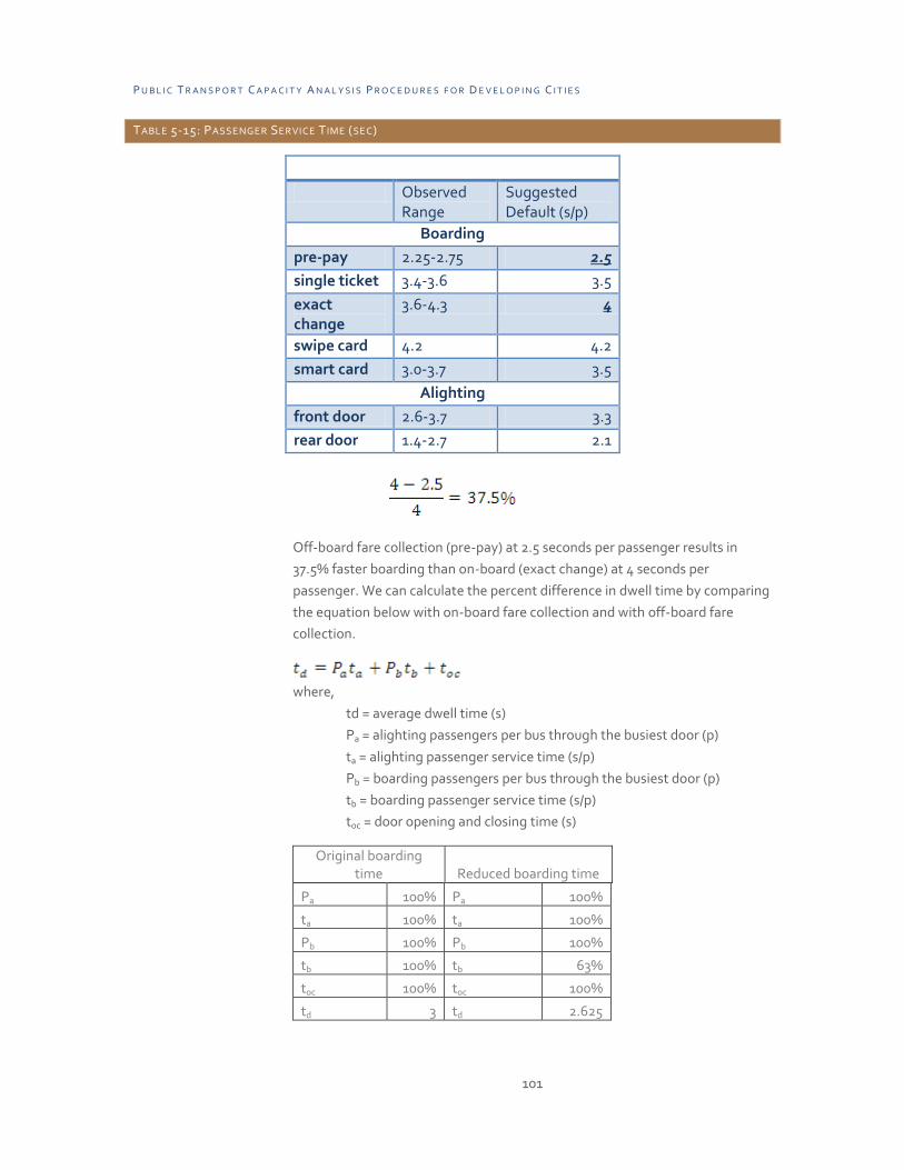
P U B L I C T R A N S P O R T C A P A C I T Y A N A L Y S I S P R O C E D U R E S F O R D E V E L O P I N G C I T I E S
101
TABLE 5-15: PASSENGER SERVICE T IME (SEC)
Observed Range
Suggested Default (s/p)
Boarding
pre-pay 2.25-2.75 2.5
single ticket 3.4-3.6 3.5
exact change
3.6-4.3 4
swipe card 4.2 4.2
smart card 3.0-3.7 3.5
Alighting
front door 2.6-3.7 3.3
rear door 1.4-2.7 2.1
Off-board fare collection (pre-pay) at 2.5 seconds per passenger results in
37.5% faster boarding than on-board (exact change) at 4 seconds per
passenger. We can calculate the percent difference in dwell time by comparing
the equation below with on-board fare collection and with off-board fare
collection.
where,
td = average dwell time (s)
Pa = alighting passengers per bus through the busiest door (p)
ta = alighting passenger service time (s/p)
Pb = boarding passengers per bus through the busiest door (p)
tb = boarding passenger service time (s/p)
toc = door opening and closing time (s)
Original boarding time Reduced boarding time
Pa 100% Pa 100%
ta 100% ta 100%
Pb 100% Pb 100%
tb 100% tb 63%
toc 100% toc 100%
td 3 td 2.625

P U B L I C T R A N S P O R T C A P A C I T Y A N A L Y S I S P R O C E D U R E S F O R D E V E L O P I N G C I T I E S
102
By going through the same calculations as previously, but using an average
dwell time of 12.5% lower than originally, we determine the capacity of the
system using off-board fare collection rather than on-board fare collection.
td = 30 * (1-.125) = 26 sec.
The ability to use rear door entry further diminishes the dwell time. A
conservative estimate of this reduction is 15%. This results in an estimate of
the mean dwell time of 22 seconds. This redetermination of dwell time
requires changes to all calculations for the baseline capacity assessment.
Calculation 1 Calculation 2 Calculation 3 Calculation 4
Bus Loading Area Capacity
Adjustment Factor Bus Facility Capacity Person Capacity
g/C 0.6 fl 1 Bl 63 Pmax 86
tc 11.1 v 200 Nel 1 B 45
td 22 c 580 fm 0.724 PHF 0.75
Z 1.28 fm 0.724 B 45.6
s 7.9 P 2,900
tom 10
Bl 63
By implementing off-board fare collection, the capacity of the single berth,
critical stop is increased from 40 to 45. The maximum passenger capacity is
2,900 customers per hour, which is exactly the design requirement. As
discussed previously, more detailed data collection at the critical stop would
be required to more precisely estimate the dwell time reduction due to rear
door entry.
Step 2.3 Assess the introduction of multiple loading areas
Introducing an additional loading area affects calculation 3 for bus facility
capacity. This, in turn increases person capacity in calculation 4. By using two
loading areas instead of one, the effective number of loading areas is increased
to 1.75
Calculation 3 Calculation 4
Bus Facility Capacity
Person Capacity
Bl 55 Pmax 86
Nel 1.75 B 70
fm 0.724 PHF 0.75
B 70 P 4,500

P U B L I C T R A N S P O R T C A P A C I T Y A N A L Y S I S P R O C E D U R E S F O R D E V E L O P I N G C I T I E S
103
Based on these calculations, by adding a second loading area, person capacity
is increased to about 4,500 passengers per hour. This is in excess of the design
requirement of 2,900.
Step 2.4 Eliminate right turn movements from bus lane
The capacity of the critical stop would be significantly improved if right turn
movements by autos were not initiated in the bus lane but rather in the second
lane. This eliminates the right turn adjustment factor and increases the person
capacity of the stop to 3,800, far in excess of the design requirement of 2,900.
Calculation 1 Calculation 2 Calculation 3 Calculation 4
Bus Loading Area Capacity
Adjustment Factor Bus Facility Capacity
Person Capacity
g/C 0.6 fl 1 Bl 63 Pmax 86
tc 11.1 V 200 Nel 1 B 45
td 22 C 580 fm .724 PHF 0.75
Z 1.28 fm 0.724 B 45
s 7.9 P 3,800
tom 10
Bl 63
Step 2.5 Increase the Allowable Standing Density
If the critical bus stop with a single loading berth is constrained to 40 buses per
hour, then a calculation can be made of the maximum standing density to
accommodate the load.
Pmax =P/ (B PHF)
Calculation 1
P 2,900
B 40
PHF .75
Pmax 97
From the table on bus sizes and densities, this indicates that the peak density
on board will be about 5 standing passengers per square meter.

P U B L I C T R A N S P O R T C A P A C I T Y A N A L Y S I S P R O C E D U R E S F O R D E V E L O P I N G C I T I E S
104
APPENDIX B - SAMPLE RAIL OPERATIONS ANALYSIS PROBLEMS
PROBLEM STATEMENT
A rail transit operating agency is expecting a 40% increase in ridership over the
next two years. The system is currently operating at a peak hour headway of 3
minutes. Calculate the current capacity and establish options that will increase
capacity to account for this anticipated increase in ridership
CURRENT OPERATING CONDITIONS
The following are the current operating conditions:
Peak direction, peak hour flow = 16,000 passengers per hour
Peak Hour Factor = 0.75
Average dwell time = 30 sec.
Standard deviation of dwell times = 12 sec
Train consist – 8 cars
Train car length – 20 meters, 3 doors per side
Acceptable loading standard – 6 persons/square meter
Advanced signal control system with train control separation of 45
seconds
Step 1 – Computer current capacity
1.1 Compute operating margin
The operating margin is:
= 24 sec
where,
tom = operating margin (s)
s = standard deviation of dwell times
1.2 Compute train station capacity
The train station capacity is:

P U B L I C T R A N S P O R T C A P A C I T Y A N A L Y S I S P R O C E D U R E S F O R D E V E L O P I N G C I T I E S
105
where,
Tl = loading area bus capacity (bus/h)
3,600 = number of seconds in 1 hour
tcs = train control separation time (s)
td = mean dwell time (s)
tom = operating margin (s) (from task 1.1)
Calculation 1
tcs 60
td 30
tom 24
Tl (bus/h) 30
headway (sec) 120
The scheduled train frequency of 20 trains per hour is less than the line
capacity of 30 trains per hour.
1.3 Estimate person capacity
The person capacity is:
where,
P = person capacity (p/h)
Pmax = maximum schedule load per traincar (see table below)
C = consist length
T = Station capacity (trains/hour)
PHF = Peak hour factor
TABLE 5-16: RAIL VEHICLE CAPACITY
Passengers/ sq.m
Rail Car Length (m) and number of doors per side
13 20 25
3 3 4
4 127 146 172
5 138 157 186
6 148 167 200
7 159 177 214
8 169 188 228
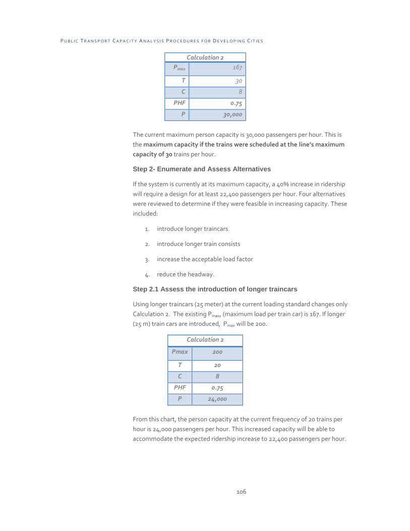
P U B L I C T R A N S P O R T C A P A C I T Y A N A L Y S I S P R O C E D U R E S F O R D E V E L O P I N G C I T I E S
106
Calculation 2
Pmax 167
T 30
C 8
PHF 0.75
P 30,000
The current maximum person capacity is 30,000 passengers per hour. This is
the maximum capacity if the trains were scheduled at the line’s maximum
capacity of 30 trains per hour.
Step 2- Enumerate and Assess Alternatives
If the system is currently at its maximum capacity, a 40% increase in ridership
will require a design for at least 22,400 passengers per hour. Four alternatives
were reviewed to determine if they were feasible in increasing capacity. These
included:
1. introduce longer traincars
2. introduce longer train consists
3. increase the acceptable load factor
4. reduce the headway.
Step 2.1 Assess the introduction of longer traincars
Using longer traincars (25 meter) at the current loading standard changes only
Calculation 2. The existing Pmax, (maximum load per train car) is 167. If longer
(25 m) train cars are introduced, Pmax will be 200.
Calculation 2
Pmax 200
T 20
C 8
PHF 0.75
P 24,000
From this chart, the person capacity at the current frequency of 20 trains per
hour is 24,000 passengers per hour. This increased capacity will be able to
accommodate the expected ridership increase to 22,400 passengers per hour.

P U B L I C T R A N S P O R T C A P A C I T Y A N A L Y S I S P R O C E D U R E S F O R D E V E L O P I N G C I T I E S
107
Step 2.2 Assess the introduction of longer train consists
Using longer train consists changes only Calculation 2. The consist length can
be increased to 10 and the calculation of capacity is shown below.
Calculation 2
Pmax 167
T 20
C 10
PHF 0.75
P 25,000
From this chart, the person capacity is increased to 25,000 passengers per hour
at the current frequency and loading standard. This increased capacity will be
able to accommodate the expected ridership increase to 22,400.
Step 2.3 Assess increasing the acceptable loading standard
If the acceptable loading standard is increased to 8 customers per square
meter, the line person capacity is computed as follows.
Calculation 2
Pmax 188
T 20
C 8
PHF 0.75
P 22,560
This is just enough capacity to accommodate the target peak load of 22,400
passengers per hour. It should be noted that operating at a higher load
standard will likely increase the stop dwell time since the passenger flow rate
on and off trains is diminished due to crowding. Given that the computed line
capacity is about 20 trains per hour, in the instant case this is not problematic.
Step 2.4 Assess increasing the service frequency
The current scheduled headway necessary to meet the demand is about 180
seconds or 3 minutes (calculated in original calculation 1). This is a frequency
of 20 trains per hour. Increasing the frequency by 40% would require
scheduling about 28 trains per hour at the current acceptable load factor. From
previous calculations, this is determined to be feasible since the flow capacity
of the line is 30 trains per hour. The number of trains per hour to meet the
requirement is:

P U B L I C T R A N S P O R T C A P A C I T Y A N A L Y S I S P R O C E D U R E S F O R D E V E L O P I N G C I T I E S
108
T = P/(Pmax C PHF )
where all terms have been defined previously
Calculation 2
P 22,400
Pmax 167
C 8
PHF 0.75
T 23
This suggests that scheduling 23 trains per hour will be able to accommodate
the passenger demand. This is less than the line capacity of 30 trains per hour.

P U B L I C T R A N S P O R T C A P A C I T Y A N A L Y S I S P R O C E D U R E S F O R D E V E L O P I N G C I T I E S
109
APPENDIX C - CASE STUDY DATA COLLECTION PROCEDURES
The report Capacity Concepts for Urban Transit Systems in Developing
Countries provides guidance on estimating transit capacity for a variety of high
capacity bus and rail transit services. In most cases, a default value is available
for use in determining transit system capacity. However, improved assessment
of capacity can be obtained by using local data. There are 8 areas where local
data would be most useful in improving the accuracy of the results.
TABLE 5-17: LIST OF PROPOSED DATA COLLECTION ACTIVITIES
1. Vehicle capacity (bus) 2. Vehicle capacity (rail)
Ticket vending machine service time 3. Rail Station headway and dwell time distribution 4. Rail Station passenger service time distribution 5. Bus Station headway dwell time distribution 6. Bus Station passenger service time distribution
These data collection efforts are grouped into two types (1) studies relating to
acceptable density on platforms and in vehicles (studies 1-3) and (2) studies
relating to the throughput capacity of passengers and vehicles (studies 4-8).
The major difference between US transit capacity analysis and that of
developing cities is determination of acceptable crowding conditions. While in
the US, densities of about 2-3 persons per square meter are determined to be
at the upper limit of acceptable crowding, much greater levels are tolerable
throughout the world. The first three data sets will help establish acceptable
ranges of static capacity on platforms and on vehicles. Operational data on
headway, dwell time and per passenger service (boarding and alighting) times
are included in the second group of data sets.
DATA SET #1 – URBAN RAIL PLATFORM CAPACITY
The objective of this data collection effort is to identify the peak capacity
based on empirical observation of actual utilization. A relatively few number of
observations, if collected at the appropriate station and at the appropriate
time can accomplish this task.
Three field measurements are proposed. The first is an estimate of the
maximum practical density of platforms in passengers per square meter. This

P U B L I C T R A N S P O R T C A P A C I T Y A N A L Y S I S P R O C E D U R E S F O R D E V E L O P I N G C I T I E S
110
would be complemented by a measure of the effective platform waiting area
which is the total platform area deducting for platform edges (about 0.5
meters), structural columns and circulation space near escalators, stairs and
elevators. Finally, during peak periods, it would be useful to determine if there
is some reduction in density at greater distances from the vertical circulation
portals.
Collection method: About four observers at the busiest station platform
during the morning and peak busiest hour would be required. This would be
done over several days. Just prior to each arriving train (in either direction if on
a center island platform), an observation of density would be made at a
number of locations along the platform. It is felt that each observer can make
two observations per arriving train. Observers would measure density at
several points along the platform to determine the average density along the
entire platform. Observers would validate the estimate of 0.5 meters from the
platform edge as the zone where passenger do not stand for waiting trains.
Alternatively, this data set might be able to be collected by reviewing
surveillance video. This would depend on the clarity of the images and the
locations of the cameras. A proposed data collection form follows as figure C.1.
The proposed analysis table to be developed from the data collection is shown
below.
TABLE 5-18: RAIL PLATFORM DENSITY DATA FORM
Date Stop
Observer Location at stop
Train Departure Time Passenger Density Train Departure Time Passenger Density

P U B L I C T R A N S P O R T C A P A C I T Y A N A L Y S I S P R O C E D U R E S F O R D E V E L O P I N G C I T I E S
111
DATA SET #2 – VEHICLE CAPACITY (BUS)
This data set involves estimating the maximum number of customers which
can be safely carried on a bus. Specifically, this effort would determine the
effective density of buses in standing persons per square meter of standing
space.
Collection method: This study might require two observers on a crowded
bus at the maximum load segment of a bus. As in the case of the rail platform
capacity, the objective is to determine the maximum observed capacity not
the mean or the distribution. If the location and time of maximum load were
determined, relatively few observations will be required to perform this study.
A data collection form is shown as Exhibit C-2.
In applying the capacity estimate, users must recognize that the boarding rate
to achieve very high loading levels may be sufficiently low as to impede
throughput capacity of the system. Data collection for this is treated in
separate data collection studies.
TABLE 5-19: BUS ON-BOARD DENSITY DATA FORM
Stop
Passenger Density Bus Departure Time Passenger Density

P U B L I C T R A N S P O R T C A P A C I T Y A N A L Y S I S P R O C E D U R E S F O R D E V E L O P I N G C I T I E S
112
DATA SET #3 – VEHICLE CAPACITY (RAIL)
This study would be similar to that of the bus capacity discussed previously. On
trainsets, it would be useful to differentiate between trains in which customers
can easily move from one car to another (open “vestibule” trains) and those in
which they cannot. The ability to “disperse” in this way tends to lower loading
diversity and thus increases effective capacity, while utilizing the protected
space between cars in this type of train (e.g., in Hong Kong, other Chinese
cities, Paris Meteor Line,) for standees also increases effective capacity.
Collection method: A data collection effort in which stationary observers on
station platforms observe the density of departing trains from the beginning
station of the maximum load segment. The data collection would focus on the
variation in density along the length of the train. The same staffing plan used
for estimating rail platform capacity (one observer for every two cars) would
be used for train set capacity. A data collection form is shown as Exhibit C-3.
This study would be similar to that of the bus capacity discussed previously.
DATA SET #4 – TICKET VENDING MACHINE SERVICE TIME
This would be a very simple study to estimate the service time distribution of
ticket vending machine transactions.
Collection method: Using a stopwatch an observation would be made of the
start time and the end time of a number of TVM transactions. If possible, the
method of payment (cash or card) would also be recorded. About 100
observations per transaction type would be sufficient to make an estimate of
the mean and distribution of the transaction time. A data collection form is
shown as Exhibit C-4.
TABLE 5-20: TVM TRANSACTION T IME DATA FORM
Date Station
Observer Start time
End Time
Transaction Duration Transaction Type
Transaction Duration Transaction Type

P U B L I C T R A N S P O R T C A P A C I T Y A N A L Y S I S P R O C E D U R E S F O R D E V E L O P I N G C I T I E S
113
DATA SET #5 – RAIL STATION DWELL TIME AND HEADWAY DISTRIBUTION
This data collection activity is to estimate the dwell time and headway
distribution of a rail transit system. This should be done at the critical stop on a
rail system – the one with the highest value of mean dwell time plus two
standard deviations.
Collection method: The data collection method is rather straightforward. The
dwell time is measured from the time that the vehicle comes to a complete
stop until the time that the train starts moving. The arrival time is the time that
the arriving train comes to a complete stop. A data collection form is shown as
Exhibit C-5.
TABLE 5-21: RAIL HEADWAY AND DWELL T IME DATA FORM
Date Station
Observer Direction
Time (train stopped) Time (train departure)
Time (train stopped)
Time (train departure)
DATA SET #6 – PASSENGER SERVICE TIMES AT RAIL STATIONS
Passenger service times are measures of the time it takes to board a passenger
under specific circumstances. The determination of passenger service times at
rail stations can be labor intensive. The data collection effort will require one

P U B L I C T R A N S P O R T C A P A C I T Y A N A L Y S I S P R O C E D U R E S F O R D E V E L O P I N G C I T I E S
114
observer for each door of a subway car. Generally, only the car determined to
be the busiest should be observed.
Collection method: The following are steps that may be used to collect field
data on passenger service times. An example of a data collection sheet is
shown in Figure C.6.
1. From a position at the rail stop under study, record the identification
number and run number for each arriving vehicle.
2. Record the time that the train comes to a complete stop.
3. Record the time that the doors have fully opened.
4. Count and record the number of passengers alighting and the number
of passengers boarding at the door.
5. Record the time that the major passengers flows end. (Note: This is
somewhat subjective but essential to correlate flows per unit of time.
This time for stragglers to board or exit should not be included.)
6. When passenger flows stop, count the number of passengers
remaining on board. (Note: If the seating capacity of the transit
vehicle is known, the number of passengers on board may be
estimated by counting the number of vacant seats or the number of
standees.) and record the time.
7. Record the times when the doors have fully closed.
8. Record the time when the vehicle starts to move. (Note: Leave time
should exclude waiting where the train must wait for a traffic signal to
turn green.
9. Note any special circumstances.
The passenger service time for each transit vehicle arrival is computed by
taking the difference between the time that the door opens and the time that
the main flow stops. The service time per passenger is computed by dividing
the number of passengers boarding (or alighting) by the total service time. A
chart showing the flow rate under varying levels of train occupancy after
departing from the station is desirable. This can be a staged variable in three
levels: all customers seated, standees at a rate of 0-2 passengers per square
meter and standees as a rate of greater than 2 passengers per square meter.

P U B L I C T R A N S P O R T C A P A C I T Y A N A L Y S I S P R O C E D U R E S F O R D E V E L O P I N G C I T I E S
115
TABLE 5-22: PASSENGER SERVICE T IME DATA SHEET
Date______ Time _______ Bus Number________ Bus Type _______ Route _____ Location _____________________________ Direction ________
Arrival Time Doors Open
Main Flow
Stops Doors
Closed Train
Leaves Ons Offs
Passengers Departing On Board
DATA SET #7 – BUS STATION DWELL TIME DISTRIBUTION
The throughput capacity of a Bus Rapid Transit System, measured in vehicles
per hour, is governed by vehicle, traffic and pedestrian and passenger behavior
at either the busiest bus stop or the most congested intersection. While it is
more likely that passenger activity at the critical stop will govern capacity, it is
possible, even with exclusive lanes that the maximum system capacity will be
determined by conflicts at intersections. These two cases will be treated
separately. The first is dwell time distribution.
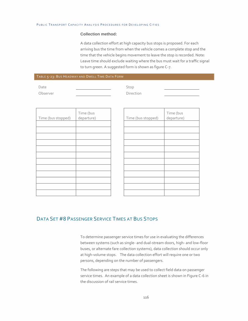
P U B L I C T R A N S P O R T C A P A C I T Y A N A L Y S I S P R O C E D U R E S F O R D E V E L O P I N G C I T I E S
116
Collection method:
A data collection effort at high capacity bus stops is proposed. For each
arriving bus the time from when the vehicle comes a complete stop and the
time that the vehicle begins movement to leave the stop is recorded. Note:
Leave time should exclude waiting where the bus must wait for a traffic signal
to turn green. A suggested form is shown as figure C-7.
TABLE 5-23: BUS HEADWAY AND DWELL T IME DATA FORM
Date Stop
Observer Direction
Time (bus stopped) Time (bus departure) Time (bus stopped)
Time (bus departure)
DATA SET #8 PASSENGER SERVICE TIMES AT BUS STOPS
To determine passenger service times for use in evaluating the differences
between systems (such as single- and dual-stream doors, high- and low-floor
buses, or alternate fare collection systems), data collection should occur only
at high-volume stops. The data collection effort will require one or two
persons, depending on the number of passengers.
The following are steps that may be used to collect field data on passenger
service times. An example of a data collection sheet is shown in Figure C-6 in
the discussion of rail service times.

P U B L I C T R A N S P O R T C A P A C I T Y A N A L Y S I S P R O C E D U R E S F O R D E V E L O P I N G C I T I E S
117
1. From a position at the transit stop under study, record the
identification number and run number for each arriving vehicle.
2. Record the time that the vehicle comes to a complete stop.
3. Record the time that the doors have fully opened.
4. Count and record the number of passengers alighting and the number
of passengers boarding.
5. Record the time that the major passengers flows end. (Note: This is
somewhat subjective but essential to correlate flows per unit of time.
This time for stragglers to board or exit should not be included.)
6. When passenger flows stop, count the number of passengers
remaining on board. (Note: If the seating capacity of the transit
vehicle is known, the number of passengers on board may be
estimated by counting the number of vacant seats or the number of
standees.)
7. Record the times when the doors have fully closed.
8. Record the time when the vehicle starts to move. (Note: Leave time
should exclude waits at timepoints or at signalized intersections
where the vehicle must wait for a traffic signal to turn green.
9. Note any special circumstances. In particular, any wheelchair
movement times should be noted.
The passenger service time for each transit vehicle arrival is computed by
taking the difference between the time that the door opens and the time that
the main slow stops. The service time per passenger is computed by dividing
the number of passengers boarding (or alighting) by the total service time.
To determine passenger service times for use in evaluating the differences
between systems (such as single- and dual-stream doors, high- and low-floor
buses, or alternate fare collection systems), data collection should only at
high-volume stops. These stops are typically downtown or at major transfer
points. The data collection effort will require one or two persons, depending
on the number of passengers.

P U B L I C T R A N S P O R T C A P A C I T Y A N A L Y S I S P R O C E D U R E S F O R D E V E L O P I N G C I T I E S
118
APPENDIX D – RAIL STATION EVACUATION ANALYSIS EXAMPLE INTRODUCTION
The computation procedure can be used to assess whether or not a particular
rapid transit station can meet the two design requirements (platform and
station evacuation) of NFPA 130. The assessment procedure involves
determining the design evacuation load, computing the platform evacuation
time and then computing the evacuation time to a safe location for a
passenger at a location farthest from an exit on the platform. The evacuation
time is the normal walking time plus any queuing time associated with level
change facilities or barriers such as door or fare collection lanes.
The example here is a side platform station with an escalator and staircase at
each end of the station. The stairs go to a fare collection concourse and then
there is another set of stairs to the outside. Figure D-1 illustrates the system.
FIGURE 5-4: RAIL STATION EXAMPLE
The following are attributes of the system being analyzed:

P U B L I C T R A N S P O R T C A P A C I T Y A N A L Y S I S P R O C E D U R E S F O R D E V E L O P I N G C I T I E S
119
Hourly volume of passengers on trains entering the station 5,600.
Peak hour factor = 0.8
Published headway = 5 minutes
Platform length = 200 m
Train capacity at 6 persons per square meter standing capacity = 193
passengers per car
Train consist length = 8 cars
Elevation to fare concourse = 9 m
Fare gates on fare concourse – 6 lanes at each of two locations
Distance from top of stairs to fare gates = 20 m.
Elevation from fare concourse to street = 9 m
Distance from top of stairs to street = 30 m.
Customer arrival rate at station = 2400/hour
Exits = 2 staircases and one escalator – one at each end of the station
(2.24 m wide)
Computation of Design Load
The design load consists of two parts (1) the design number of passengers
awaiting trains and (2) the design number of passengers on the next arriving
train at the station.
Awaiting Passengers
The design number of passengers waiting on the platform is the maximum
number of passengers who will be waiting for a train. It is computed as the
arrival flow rate per minute adjusted upward by the peak hour factor
multiplied by the maximum time between trains. The maximum arrival time
between trains is computed as 12 minutes or twice the headway, whichever is
larger. The basis for this is that on long headway services (over 6 minutes
published headway) the evacuation system is designed for a service where a
single train is missing from the schedule. On short headway services (6
minutes or under) the evacuation system is designed so that the maximum
time between trains is 12 minutes.
For the design problem:
Arrival rate in 15 minutes = Hourly arrival rate/(60 * peak hour factor) *
max(12, 2 * headway)
Awaiting Passenger Design Load = (2400/(60 * .75) *12 = 640
Arriving Passengers
The arriving number of passengers on the next train is computed by
determining the hourly flow of passengers on trains arriving at the station
during the peak hour, adjusting this result upward by the peak hour factor then

P U B L I C T R A N S P O R T C A P A C I T Y A N A L Y S I S P R O C E D U R E S F O R D E V E L O P I N G C I T I E S
120
dividing by the number of scheduled trains during the hour. This calculation
provides the number of customers on the next train during the peak 15
minutes under normal operation. The recommended practice is to increase
this number by two to account for a service interruption where a train is
eliminated from the headway. The maximum arriving passenger design load is
the maximum train capacity.
Arriving Passenger Design Load = (Arriving passengers per hour / (trains per
hour * PHF) ) *2
Arriving Passenger Design Load = (5,600/(12 * .8) ) * 2 = 1,166
Total Design Load
The total design load for platform evacuation is the sum of the design load of
awaiting passengers and arriving passengers. This is 640 + 1,166 = 1,806
passengers.
Test 1- Platform Evacuation Assessment
There are 2 staircases and 2 escalators at each end of the platform. The design
requirement is to assume that one of the escalators is out of service due to
maintenance requirements. Using capacity estimates in Error! Reference
source not found., the estimated egress capacity is illustrated in Error!
Reference source not found. below. This suggests that the evacuation rate
from the platform is 454 passengers per minute. It would take just under 4
minutes to evacuate the platform under these conditions. Therefore, the
design meets test 1 which requires platform evacuation in 4 minutes or less.
TABLE 5-24 : FLOW RATES OF MEANS OF EGRESS IN SAMPLE PROBLEM
width (m)
capacity per unit width
(Pass/m/min)
Effectiveness Flow (pass/min)
Effective Flow (pass/min)
Stair 1 3 63 1 189 189
Escalator 1 1.2 63 1 75.6 76
Stair 2 3 63 1 189 189
Escalator 2 1.2 63 0 75.6 0
Total 454
TEST 2 - STATION EVACUATION ASSESSMENT

P U B L I C T R A N S P O R T C A P A C I T Y A N A L Y S I S P R O C E D U R E S F O R D E V E L O P I N G C I T I E S
121
Walking Time
The station evacuation test requires that all occupants be able to evacuate to a
safe location within 6 minutes. The travel time to a safe location is the sum of
the travel time without any queuing delays plus to queuing delays caused by
restrictions on capacity at stairs and escalators, faregates and doors.
The normal travel time of the person leaving from a point on the platform
farthest from the street is computed. Error! Reference source not found.
below illustrates the computations.
TABLE 5-25: T IME FROM PLATFORM TO EXIT
Distance (m) Speed (m/min)
Time (min)
platform to stairs 40 61 0.66
climb stairs 9 15 0.60
stairs to fare gates 20 61 0.33
concourse to stairs 30 61 0.49
stairs to street 9 15 0.60
Total 108 2.68
The platform to stairs time assumes that an occupant is at the farthest possible
distance from a staircase or escalator. The maximum unimpeded time is about
2.7 minutes.
Waiting Time
A separate queuing assessment is made at each location where free flow is
restricted. The four restricted spaces are described in the table below.
The first part is computing the waiting time at the platform exit of the last
exiting passenger. This is the platform evacuation time (computed at 2.68
minutes) minus the walk time of the last passenger to the platform exit. (This
assumes that there will be queue at the platform exit even after walking to the
exit from the point farthest from the exit.
The next barrier is the fare exit barrier. The delay time for this barrier is the
concourse load divided by the fare barrier exit capacity. The design number of
exiting passengers is 1806. The exiting flow capacity of the faregates is 50
passengers per minute. (from table xx). With 8 exit faregates, the time to
evacuate all passengers is 1806/(8 * 50) = 4.5 minutes. The delay time

P U B L I C T R A N S P O R T C A P A C I T Y A N A L Y S I S P R O C E D U R E S F O R D E V E L O P I N G C I T I E S
122
The waiting time at the fare barrier gate by the last exiting person is the fare
barrier flow time minus the platform clearance time of 2.34 minutes.
If the flow capacity of the exit faregates were higher than that of the platform
exit, then the delay time of the last passenger at the faregate would have been
0.
The next step is to assess the delay time at the stairs from the concourse to the
street level. At each of the two exits there is a staircase 3 meters wide. No
escalators are used. From the calculation of the exit capacity from the stairs
from the platform to the concourse, the maximum flow time at the base of the
exit stairway is:
The waiting time at the concourse exit by the last evacuating passenger is
g1
The total exit time is the sum of the unimpeded walk time plus the sum of the
delay time at the three points of restricted flow – the stairs from the platform
to the concourse, the faregates and the stairs from the concourse to the street.
P U B L I C T R A N S P O R T C A P A C I T Y A N A L Y S I S P R O C E D U R E S F O R D E V E L O P I N G C I T I E S
123
This egress system does not meet the NFPA standards. Remedies which could
be considered include:
Adding an emergency staircase from the platform to the street. This
would bypass two of the barriers – the faregate and the second
staircase.
Making exit staircases wider
Increasing the exit capacity through the faregates. This might be done
by adding an emergency bypass gate at the faregates. This would
increase flow and reduce additional delay time at the faregates.
This discussion is intended to be a preliminary treatment of underground
station evacuation requirements. The NFPA requirements should be consulted
for more complex treatments such as center island platforms and multiple
station access points.
Emergency evacuation provisions are an essential consideration in capacity
analysis and station and terminal design. Specific procedures and
requirements will vary among countries. Design and performance standards
for emergency evacuation in the United States provide a guide in this effort.
Transport Division
Transport, Water and
Information and Communication
Technology Department
The World Bank
1818 H Street NW
Washington DC 20433
USA
www.worldbank.org/Transport