public journal of transportation - university of south florida
TRANSCRIPT


Volume 13, No. 2, 2010ISSN 1077-291X
The Journal of Public Transportation is published quarterly by
National Center for Transit ResearchCenter for Urban Transportation Research
University of South Florida • College of Engineering4202 East Fowler Avenue, CUT100
Tampa, Florida 33620-5375Phone: (813) 974-3120
Fax: (813) 974-5168Email: [email protected]
Website: www.nctr.usf.edu/jpt/journal.htm
© 2010 Center for Urban Transportation Research
PublicTransportation
Journal of


iii
Volume 13, No. 2, 2010ISSN 1077-291X
CONTENTS
Tax-Free Transit Benefits at 30: Evolution of a Free Parking OffsetStuart M. Baker, David Judd, Richard L. Oram .............................................................................1
Planning for Demographic Diversity: The Case of Immigrants and Public TransitEvelyn Blumenberg, Alexandra Elizabeth Evans .............................................................. 23
Are Suburban TODs Over-Parked?Robert Cervero, Arlie Adkins, Cathleen Sullivan ..........................................................47
Effect of Variable Bus Speeds on Bus Network DesignNicole Foletta, Miquel Estrada, Mireia Roca-Riu, Pere Martí...............................................71
Water-Transit Services in Dubai-UAE: User and Operator Survey Development and Quantitative AnalysisMohammad Nurul Hassan, Yaser E. Hawas, Faisal Ahmed, Munjed Maraqa, Md Bayzid Khan ........................................................................................................................................93
Investment Decision Making for Alternative Fuel Public Transport Buses: The Case of Brisbane TransportAnish Patil, Paulien Herder, Kerry Brown ................................................................................... 115


1
Tax-Free Transit Benefits at 30
Tax-Free Transit Benefits at 30: Evolution of a Free Parking Offset
Stuart M. Baker, Stuart M. Baker, Inc. David Judd, Transportation Consultant Richard L. Oram, Oram Associates, Inc.
Abstract
Tax-free employee transit benefits emerged in the 1970s along with monthly pass plans and evolved over a 30-year period to be an important part of transit market-ing, transit revenue, and traffic mitigation strategies. Transit benefit plans succeeded partly because they are an “offset” to employer-provided tax-free parking, an integral part of transit’s market context in theoretical and practical terms. First authorized in 1984 at a tax-free monthly maximum of $15, transit benefit legislation was expanded numerous times and now allows a monthly maximum of $230, equaling tax-free parking. Indicating the effectiveness of workplace market development, transit ben-efit impacts greatly exceed what comparable changes in transit fare levels suggest. A series of innovations for delivering transit benefits and unique public-private relation-ships provided ever-better ways to meet employer needs, and will continue to evolve as transit fare collection methods advance.
Introduction This paper summarizes underlying concepts, history, impacts, and status of “tran-sit benefits,” a tax incentive strategy for involving employers in efforts to reduce traffic congestion, greenhouse gas emissions, and energy use, by promoting public transit use. Transit benefits —tax-free employer-provided benefits for public trans-port—is the government tax policy in which transit fares are a tax-free employer-

Journal of Public Transportation, Vol. 13, No. 2, 2010
2
and/or employee-paid benefit, delivered using an array of programs and services provided to employers. Transit benefits are formally authorized under Section 132(f) of the United States (U.S.) Internal Revenue Code.
Economics and Free Parking The first employer-based transit programs arose in the 1970s as transit agencies began using monthly passes and sought primarily to have employers be supple-mental pass sales outlets. For example, after Massachusetts Bay Transportation Authority monthly passes were introduced, their popularity and the limited num-ber of public sales outlets led many employers to become “private” sales outlets for their employees. As passes and employer-based sales spread to other cities, employers also were encouraged to pay for passes in whole or part. Used infor-mally for years before, employer fare discount plans – transit benefits – were first authorized by the Tax Reduction Act of 1984, with use limited to employer subsidy of no more than $15 per month. Their use became popular in the late 1980s, and through the 1990s appeal expanded rapidly as the tax-free maximum rose and an employee-paid option and new administrative services were added.
Due to the tax savings and employee appeal, transit benefits are now used to varying degrees in every U.S. city. They are a standard employee benefit in New York, Chicago, Boston, San Francisco, Seattle and elsewhere. Reviewing pertinent economic theory and transit’s overall market context helps understand how this was achieved, and its importance.
National Personal Transportation Survey data show that for all purposes, free parking is available for 99 percent of daily trips (Hu and Young 1998). The impact of free or partly-subsidized work-based parking (Shoup and Pickrell 1980; Wilson and Shoup 1992; Wilson and Shoup 1997) is one reason transit benefit tax poli-cies were first established and later expanded by the government, and embraced by employers. The public policy behind transit benefits can be understood using the economics principle “theory of the second best,” formalized by economists Richard Lipsey and Kelvin Lancaster in 1956. Free or subsidized parking is a market “distortion” yielding social “externality” costs borne by third parties. These costs include pollution, congestion, inefficient energy use, and many other direct and indirect impacts of auto-focused policies. Density, largely reflecting the amount of land devoted to parking, often defines the level of transit service that is viable. Hav-

3
Tax-Free Transit Benefits at 30
ing less transit service provided than otherwise might be can also be considered an economic externality.
It is hard to understate the role of workplace parking policies in urban transporta-tion. Free parking is a potent market distortion with profound effects on transit demand, auto ownership, land use patterns, and home ownership decisions, such as commuting distance or the choice between an apartment or single family resi-dence. In short, it promotes low-density lifestyles that can even be linked (Owen 2009) to decisions about family size. Economists say that if market distortions cannot be corrected directly, as a “first best” solution, introducing a “second best” solution is appropriate. Transit subsidies in general and specifically transit-promoting tax incentives focused on the workplace are thus justified as “correc-tions.”
Free parking is difficult to address and not a solely American practice. In Canada, England, and Australia where it is technically not authorized as a tax-free benefit, for example, it is still widely provided by employers. For tax purposes, owing in part to many direct and indirect ways parking subsidies are provided in different settings, it is impossible to consistently identify parking costs or benefits, which makes the provisions largely ineffective. For example, it is hard to place a value on parking spaces adjacent to a building, especially if the number of spaces or building setback is mandated by municipal code, or when customers and employees share parking. For tax purposes, free and discounted employee parking is a ubiquitous but elusive practice, especially in suburban settings. Even when employers do not provide parking, the many other external/social costs of auto use justify favorable tax policies for transit users, and given the determinant role of commuting deci-sions, a focus on employers is most effective.
Parking subsidy clearly promotes auto use, but existence of auto subsidies (even just on-site parking spaces) also makes transit benefits attractive to employers. For employee benefits, employers are very sensitive to equity and strongly favor benefits that can be used by all employees. With many employees already receiv-ing free or discounted parking, many employers embraced transit benefit plans as they became administratively practical, partly due to pressure from transit-using employees wanting commuting benefits “equalized.” The 30 years of U.S. experi-ence with transit benefits shows that transit benefit plans reflecting employer sensitivities—which foremost means they reflect employer concerns for simplicity and equity—can be readily and successfully marketed. This also means that the theory of the second best can work.

Journal of Public Transportation, Vol. 13, No. 2, 2010
4
Transit does not serve many employment sites, and in general far fewer employees are offered tax-free transit than parking even where transit service exists. Yet in some cities large shares of transit users get transit benefits. For example, a 2006 study (Bay Area Rapid Transit District 2006) reported that 43 percent of San Fran-cisco’s Bay Area Rapid Transit riders work for employers offering a transit benefit plan, an increase from 39 percent in 2003. The 2006 measure is 63 percent when the data are adjusted to reflect only employed peak-period commuters. A series of innovations caused this important change in the U.S. transit industry.
Experience to Date U.S. transit benefits are provided in two alternate ways, and a third combines the two. The initial application was “employer subsidy” for transit, with the practice directly analogous to employer-paid (or provided) parking, where the expense is borne by the employer.
The more recent and popular application has employees paying transit fares using before-tax salary; deductions are made from gross salary before income or payroll taxes are applied. This is a “pre-tax benefit” in the U.S. and “salary sacrifice” else-where in the world.
The third or combination alternative is “fare sharing.” Here, the employer pays part of the benefit as a tax-free subsidy and the employee pays the remainder with pre-tax salary. In practice, beyond the basic options, employers adopt numerous variations to make their plan consistent with the employer’s overall benefits and “corporate culture.” For example, employers might subsidize half of employee fares or a flat amount such as $30 per month, or require participation for a certain number of months. U.S. law allows many variations, which is surely an important element in the acceptance the programs have had.
Table 1 summarizes key junctures in the evolution of transit benefits. It was for-mally established in U.S. tax code in 1984, partly to clarify the status of informal practices known as “employer pass plans” existing in some cities. Some cities had large pass plans, and it is notable that these cities had basically one transit opera-tor, in contrast to other cities with multiple providers. In pass plans, employers buy monthly passes (the programs being limited to passes is important) and sell them to employees, sometimes at a discount ,with the benefit tax-free. The pro-cess can be complex; employers need to order the correct number of passes (often more than one type), receive and store them, distribute them monthly, receive

5
Tax-Free Transit Benefits at 30
payments/co-payments from employees, return unused passes, pay the transit operator (consignment sales were most common, with monthly reconciliation), etc. Employees often change their requirement, e.g., for a vacation or month with business trips or holidays. These administrative requirements gave pass plans lim-ited use, except in a few cities such as Seattle and Boston, where they did become popular with larger employers. Cities with complex transit networks (those with multiple modes, operators, and zonal fares, as in New York and Chicago) did not have pass programs, mostly due to the even greater burden an employer would have. Employers with staff in multiple cities often could not provide comparable benefits to all employees, so these employers most often did not participate. Overall, few employers participated. Employer pass plans also are costly for transit agencies to operate.
Table 1. Highlights of U.S. History with Transit Benefits
1970s Employer pass programs emerge
1984 Legislation “codifies” use of transit benefits, allowing $15 per month
maximum benefit (“cap”); limited to employer subsidy
1987 First transit voucher plan implemented in New York
1990 First Eco-Pass plan implemented in Boulder and Denver
1990s Self-supporting national transit benefit services emerge
1991 Inflation adjustment raises transit benefit cap to $21
1992 New legislation raises cap to $60 per month
1995 Inflation adjustment raises cap to $65
1998 Employee-paid pre-tax payroll deduction feature added
2000 Executive Order mandates transit benefits for Federal employees
2002 Monthly maximum benefit raises cap to $100
2005 Inflation adjustment raises cap to $105
2007 Inflation adjustment raises cap to $110
2008 Inflation adjustment raises cap to $115
2008 City of San Francisco adopts transit benefit ordinance
2009 January: Inflation adjustment raises cap to $120
2009 February: New legislation (2009 legislation limits the increase for two years)
raises cap to $230, matching the cap for tax-free parking.
2009 Transit benefit ordinances adopted in California by City of Richmond, San
Francisco Airport Authority, City of Berkeley

Journal of Public Transportation, Vol. 13, No. 2, 2010
6
Despite limited use, the untapped promise in this area and market research find-ings showing over 80 percent of drivers entering lower Manhattan received some type of employer auto subsidy (most often free or subsidized parking) led transit agencies in New York to seek clarification of the practice in the tax code. As a result, the 1984 legislation defined the transit benefit as a “deminimus benefit” and established its maximum value at $15 per month. Focused program development efforts began in New York City in 1984.
Regulations following the 1984 legislation allowed the benefit to be provided as passes, tickets, tokens, or vouchers. Allowing vouchers (they had not yet been used) reflected a desire to devise transit benefit plans in cities with more than one transit provider, e.g., New York, San Francisco, Philadelphia, and Chicago. Vouch-ers were seen as a way for employer participation to be widespread and even simple for most employers. Focus groups found administrative simplicity vital to employer consideration of any fringe benefit. This supported the decision to develop vouchers, as an employer pass plan in New York could require employers to handle dozens of fare instruments for the many rail, bus, and ferry services and different pass types and fare zones. In contrast, vouchers are script (in most cities, specialized bank checks) that employers simply buy and give to employees, who redeem them where all participating operators’ passes or tickets are sold. That they do not expire from month-to-month also simplified administration. Figure 1 illustrates a transit voucher currently in use.
Figure 1. Transit Voucher
Focused purely on transit subsidy and piloted by a multi-agency effort of New York City transit operators as a Federal Transit Administration demonstration project, the first voucher plan began in 1987. The administrative advantages and simplicity of vouchers enabled the plan to quickly find success. Compared to employer pass

7
Tax-Free Transit Benefits at 30
plans that sought primarily to have employers be pass sales outlets, private sales outlets were not needed in New York , and the voucher plan sought what employ-ers could uniquely provide: subsidy and tax benefits. It became clear that asking employers to be sales outlets and provide subsidies meant that, in most cases, they simply did not participate. Many transit pass plans also had minimum order quantities, which meant, by definition, that small employers could not participate. In contrast, according to the U.S. Census Bureau’s Statistics on U.S. Businesses, 71 percent of U.S. employers have fewer than 20 employees.
While some cities developed local programs, scale economies and employer willingness to pay nominal fees led nationally-focused transit voucher services to emerge. Within a few years, “TransitChek®” and “Commuter Check®” vouch-ers served over a dozen cities. Transit agencies gained rides and revenue, and privately-operated programs meant transit agencies had little if any expense. Many provided marketing assistance, e.g., posters in buses and trains. The cost to transit agencies of receiving and processing vouchers was generally minimal, usu-ally negligible. As the vouchers were bank checks, they most often were received and deposited by private sales outlets (e.g., groceries), with transit agencies not even receiving them.
Vouchers had new features reflecting employer needs (Oram 1990). As a “least common denominator” instrument, they were something all employees could use. Employers usually did not have to worry about which one was for which employee; they were essentially interchangeable and did not expire for over a year. The plans were not limited to monthly pass users and avoided employee co-payment, a seri-ous limitation of most employer pass plans. With vouchers redeemable for any fare type, less-than-regular and even infrequent riders participate, which is critical for many reasons. Keenly sensitive to equity, most employers simply will not adopt programs if only some transit-using employees can participate.
Even if an employer adopts a program limited to passes, it yields far less new rid-ership than a broader plan. Research found induced transit trips resulting from voucher plans most often reflecting non-users becoming occasional users and occasional users riding more (Metropolitan Transportation Commission 1995). Instances of non-users converting to regular users were rare. Consistent with this, a “transit rider life cycle” was observed (Perk et al. 2008); on-board surveys found that most riders began using transit for occasional work trips, and if they continued riding—many did not—they increased their use and sometimes added
Journal of Public Transportation, Vol. 13, No. 2, 2010
8
off-peak trips. The studies also suggested transit benefits would diminish turnover (rider attrition), which was found to be significant.
Transit commuters are typically thought to ride every day, but U.S. and Canadian studies found less-than-regular riders comprising a large and often majority share of transit commuters. A paper (Oram and Stark 1997) published by the U.S. Trans-portation Research Board reported these “surprising” findings and suggested that transit marketing, advertising, pricing levels, and fare structure needed rethinking. A national study (Federal Highway Administration 1997) stated, “Those who say they use transit to get around constitute about 27 percent of transit riders, with usual auto users who use transit only on an occasional basis constituting about 62 percent.”
To include these users, transit benefit plans cannot be limited to passes. For example, if a pass costs $50 and an employer provides a $20 subsidy, employees do not save anything until $30 in rides is taken; hence, most employees are left out. Additionally, someone who already rides that much is unlikely or even unable to ride much more. This suggests, counter-intuitively and unlike most employer pass plans, that the most important target for a transit benefit plan is the less-than-regular and infrequent rider market segments. The role of infrequent riders means a large share of employees can participate in programs not limited to passes. Rather than serve relatively few and thus have less appeal to employers, vouchers can serve most employees; over a period of a year, virtually all employees may be able to use a $20 voucher, for example. This is vital, as most employers won’t adopt ben-efits serving few employees. Thus, serving infrequent riders is critical and arguably the core reason that transit benefits gained wider use. Again counter-intuitive, being able to serve the large number of irregular or even infrequent users “drives” the success of a transit benefit initiative.
The market data above on the role of infrequent riders, supported by transit benefit program experience, suggest that if infrequent use is not a primary focus, employee participation will be less than half of what it otherwise would be. And assuming at least five times the number of employers join simpler and broader programs (based on experience, this is a conservative estimate), one can conclude that a plan that accommodates infrequent users as well as pass users would have at least 10 times the participation of a plan limited to regular (pass) users. Fur-thermore, as regular riders are far less able to expand transit use, the impact of a broader program will be far more than a factor of 10.
9
Tax-Free Transit Benefits at 30
Being simpler, more equitable and applying to the “first dollars” of fares, vouch-ers profoundly increased interest in and impacts of employer transit programs. It was a breakthrough that re-wrote the book. Voucher plans enrolled thousands of employers in large cities and created a new ridership and revenue tool for medium-sized and smaller cities. Vouchers changed a peripheral idea to an important part of transit marketing and revenue generation strategies, and employer benefit packages. Having the private sector operate the programs and provide substantial marketing support also was critical and perhaps unique.
Compared to the pass plans that generally appealed to relatively few and mostly larger employers, vouchers appealed to far more and were notably effective in drawing thousands of small employers, where there was previously no participa-tion. As employers need to stay competitive with their peers regarding benefits and are especially interested in low-cost benefits, added participation and vali-dation of the benefit by smaller and medium-sized employers prompted larger ones to also enroll—a virtuous cycle began. Like infrequent riders, discovering the role of smaller employers was another key to the expansion of U.S. transit benefit programs.
Having found market appeal, transit benefit advocates succeeded over the years in expanding the enabling legislation. In 1991, the $15 limit became $21 as an inflation adjustment was adopted due to the demonstrated interest and result-ing political pressure. Legislative changes brought further increases and massive broadening of the provisions via the 1998 introduction of the employee-paid pre-tax option. One of the changes established a cap on parking benefits, which was previously tax-free at any level. An Executive Order signed by President Clinton established transit benefits for Federal government employees. A series of inflation adjustments brought the cap to $115 in January 2008 and $120 in January 2009, and as part of the 2009 Economic Stimulus Bill, transit and parking benefits were equalized at $230 (at least until 2011). It took 25 years, from 2004 until 2009, for the authorized transit benefit cap to reach parity with parking.
Table 1 noted EcoPass plans appearing in 1990. EcoPass began in Boulder and Denver as a way to provide discounted fares, primarily for university students (in some cities, it is called UniPass) but later for employers as well. They are almost always limited to settings with one transit operator. EcoPass entails the university or employer purchasing, under contract with the transit agency, annual transit passes for all of its students or employees, at a discounted price. With free access, experience has shown (Brown et al. 2003) that EcoPass generates considerable

Journal of Public Transportation, Vol. 13, No. 2, 2010
10
new ridership, regardless of a rider’s trip frequency. It does not build revenue, at least initially, and can lead to added service requirements, but is very popular. The EcoPass concept appeals partly because it entails no ongoing administration. The initial intent was that the employer would subsidize the annual contract amount, which would be a tax-free subsidy, but in many cases employers devised an employee monthly co-payment so that the employer removed or diminished its cost. The co-payment made EcoPass somewhat like the traditional employer pass plan, though it was less than the normal pass cost. As the law changed, some employers allowed the employee payment as a pre-tax deduction. EcoPass is pri-marily a marketing and fare collection plan and secondly a transit benefit option and can have serious long-term net revenue implications (e.g., revenue growth less added service requirements, and resistance to higher fares by employers). It was important to drawing employers into transit programs, but except at universities, is not likely to expand considerably.
Newer ServicesWith the market established, other innovations were equally important in expanding transit benefit use and will be increasingly important going forward. As internet commerce emerged, new transit benefit programs further tailored the transit benefit to employer needs. Vouchers did not appeal to many larger employers (although many do use them, e.g., the U.S. Government) and also were not well suited to needs of employers with offices in different cities. For these, “on-line/at-home” programs were devised. Many larger and multi-site employers disliked having to purchase, store, and distribute vouchers (which varied by city) and wanted streamlined procedures to match employee fares with their payroll systems. On-line programs, using websites taylored to reflect particular provisions of the employer, enabled employees to specify their ticket/pass/voucher need for the upcoming month or quarter, or set a standing order. Program administrators, again self-supporting private businesses, provided the employer with a “payroll file” tailored to the employer’s needs. When the employer made the payroll deductions and paid the administrator for the fare media and service fee, the administrator mailed the passes or vouchers to employee homes. Some employers pre-pay an estimated amount to avoid delays.
The convenience of “at-home” programs gave transit benefits further market pen-etration, especially with larger employers. That the cost of this enhanced service exceeded voucher fees was generally a subordinate consideration. Some employ-

11
Tax-Free Transit Benefits at 30
ers, however, opted for a voucher-only at-home service; as vouchers did not need to be mailed every month, this was very economical. Based on a cost-per-fulfill-ment rather than percentage of face value as vouchers involve, at-home programs gained a cost advantage as the monthly cap rose. A “direct load” to smart cards is another and increasingly important feature.
Further growth resulted by integrating transit benefits with “third-party adminis-trator” (TPA) services. TPA companies administer payroll, health, retirement, and similar plans. Most large employers and many medium-sized and smaller ones use TPAs. By drawing these “major players” into the transit benefit field, one can say the transit benefit “came of age.”
Smart cards presented challenges but ultimately resulted in another opportunity to expand transit benefits. The Washington, D.C. transit system led the way in this area. Essentially, transit benefit value must be transmitted electronically to the smart card administrator and each employee’s card. The on-line/at-home plans did this, but not all employers found this model attractive relative to vouchers. In general, integrating transit benefits with smart cards entailed significant complexi-ties, as (like the early pass plans) most employers do not want to be involved in details of employee fare payments. One informed observer noted that smart cards and transit benefits were on a collision course. To avoid this, smart cards can be integrated with transit benefits using a “virtual voucher” or “e-voucher” to marry the appeal and efficiency of vouchers with the conveniences of smart cards and the internet.
An e-voucher entails the employee receiving a unique “voucher” number for one-time use on a specialized website, where the employee applies the value for individual rides, a pass, etc. This meant the employer’s role could be even simpler than with paper vouchers, as virtual vouchers are electronic and do not necessarily require anything to be distributed. This is particularly attractive to employers who do not use TPAs or do not want or cannot have an on-line ordering platform inte-grated with their payroll system. The e-voucher can have lower costs for employers and transit agencies.
Being electronic, e-vouchers are not physically redeemed. The value is “contained” in the number and not on a piece of paper where it may be printed. E-vouchers can even be distributed simply as e-mail messages. Another important feature of an e-voucher is that customer service is handled either by the transit benefit ser-vice provider or smart card administrator, with employers essentially uninvolved. As smart cards are used in more cities, e-vouchers may become a core way to

Journal of Public Transportation, Vol. 13, No. 2, 2010
12
administer transit benefits, replacing paper vouchers, at-home delivery, and other means. An e-voucher can avoid the transit benefit/smart card collision.
Debit cards are another way to deliver transit benefits in cities where fare vending machines, ticket-by-mail plans and smart cards are used. The initial personalized debit cards met market resistance. Some vendors, often TPAs using debit cards for other benefits, felt debit cards would be the best way to offer transit benefits, but their limited initial “pick up” affirms the key employer concerns for simplicity and universality. Unlike vouchers, personalized debit cards associate a specific person and card number with the requested value and “re-loads.” The debit cards also required personal user information, which raised privacy and security issues. They also entailed more customer service than vouchers.
Initial efforts with personalized debit cards proved that they would not be a sole solution for employers or employees, and they did not gain significant market share. Furthering this were Internal Revenue Service regulations issued in 2006 on the use of transit benefit debit cards. The regulations phased-in restrictions to limit and ultimately (in 2011) preclude their use in situations where employees might receive cash from the card, e.g., retail sales outlets. This made debit cards less attractive than vouchers, the majority of which are redeemed at retail outlets, or an at-home service. Customer service issues also arose, many related to the non-transferable nature of personalized cards, which is not a factor for vouchers. Many of the TPA vendors withdrew their cards, but others with expertise in the transit industry made their programs fully compliant and efficient for employers and users.
To avoid many of the personalized card issues, a streamlined non-personalized debit card (“stored value card”) was devised; this is more popular but still has re-loading, customer service, and other complexities. When used at transit fare vending machines, debit cards also impose 2-3 percent transaction fees on transit agencies and, as they are discarded after use, they create trash and environmen-tal concerns. It remains unclear how important debit cards, in any form, will be to the future of transit benefits. They are less attractive when most transit fares are bought at retail outlets, but are needed in some cities and will likely be more attractive as automated fare collection serves more cities and users.
Transit fare collection procedures vary greatly from city to city. This adds to the varying preferences that employers have and means that a single solution for administering transit benefits likely does not exist. What is efficient or attractive in one city is often less attractive or unworkable in another. What one city sees as a cost, such as debit card transaction fees that can be avoided with a retail sales net-

13
Tax-Free Transit Benefits at 30
work, may be accepted in another city as just a cost of automated fare collection and offset by those benefits. Going forward, debit cards with embedded chips, cell phone, and other emerging payment technologies may be important in fare col-lection, which means they also would gain use in transit benefit plans. As with the current options, each will have pros and cons. Like employer-supported parking, transit benefits likely will always be provided in numerous ways. Transit benefits will hopefully become just as integrated as parking is as an employee benefit.
Table 2 presents the sequence in which the transit benefit administrative options emerged. Most notable is their evolution regarding the employer’s key concern: simplicity and administrative ease. Increased efficiency and thus participation resulted when vouchers became the primary mechanism. EcoPass provided an annual option. Further efficiency resulted as on-line programs emerged to meet needs of larger and multi-site employers, and bring in TPAs. Debit cards are needed and work well in some cities. Serving smart cards will yield further efficiency by allowing the “tangible” elements and activities to disappear.
Table 2. Evolution of Transit Benefit Administration Options
1970s: Employer pass plans
1987: Transit vouchers begin in New York
1990: First EcoPass program begins
1990s: Transit vouchers used nationally
1999: At-home programs emerge
2000: Third-party administrator programs emerge
2004: Debit card programs begin
2006: E-voucher program begins
Tables 3, 4 and 5 offer opinions on the relative appeal, market impacts, and prom-ise of the options now used. While vouchers gave transit benefits broad appeal, integrating transit benefits with the constantly-evolving technology of fares and benefits quickly became important and will be increasingly vital as transit ben-efits reach ever-more employees. In sum, a self-supporting industry with robust services emerged to meet diverse employer needs and provide tax savings and transit incentives to reduce auto use where such efforts are most effective, at the workplace.

Journal of Public Transportation, Vol. 13, No. 2, 2010
14
Table 3. Relative Appeal of Transit Benefit Administration Options
Employer Pass Plans: Larger employers, generally located in one city
Voucher Plans: Initially smaller employers, subsequently larger
EcoPass Plans: Generally universities and larger employers
At-Home Plans: Generally larger employers, often multi-city
Third-Party Administrator Plans: Medium to larger employers, all cities
Debit Card Plans: Large employers, often multi-city
E-Voucher Plans: Employers in cities with smart card fare collection
Table 4. Relative Impact of Transit Benefit Administration Options
Employer Pass Plans: Ground-breaking option but limited appeal and
only in some cities
Voucher Plans: Rapid growth into new markets, validated concepts
EcoPass Plans: Substantial impact on ridership in a few cities
At-Home Plans: Substantial appeal in most major markets
Third-Party Administrator Plans: Substantial appeal in most major markets
Debit Card Plans: Appeal limited to cities where credit/debit cards
are accepted
E-Voucher Plans: To be determined as smart card fare collection
expands
Table 5. Future of Transit Benefit Administration Options
Employer Pass Plans: Use has declined and will continue to
Voucher Plans: Unclear; large markets still not penetrated but
conversion to new options occurring, esp. in automatic
fare collection cities
EcoPass Plans: Unlikely to expand except in university or similar settings
At-Home Plans: Substantial growth likely
Third-Party Administrator Plans: Substantial growth likely
Debit Card Plans: Substantial growth likely as automatic fare collection
expands
E-Voucher Plans: Likely very important as smart card fare collection
advances

15
Tax-Free Transit Benefits at 30
Impacts of Transit BenefitsConceptually, impacts of transit tax incentives can be projected using standard measures of fare change sensitivity, or elasticities, observed from decades of fare changes. Summarizing experience with price changes, Litman (2009) notes work trips are especially insensitive to fare changes, reporting elasticities ranging from -0.1 to -0.19. Assuming an average of -0.15, a 10 percent fare change would lead to a 1.5 percent change in ridership. (The minus sign indicates the inverse relation-ship between fares and usage.) The -0.15 figure, however, is an average; different measures for bus vs. rail, small vs. medium vs. large cities, urban vs. suburban settings, fare types, rider categories, and other factors have been determined. In considering transit benefit impacts, it is important to consider that a -0.15 average figure also does not reflect significant differences in sensitivity shown by regular vs. infrequent riders, e.g., a rider changing all trips to transit or just a few (Lewis and Williams 1999; Tromer et al. 1995; Oram 1988, 1994). Also notable is that fare change sensitivity is generally inverse to city size, suggesting transit benefits can have more impact where auto use is greater. Still, the -0.15 work trip elasticity can be used when considering changes over broad areas.
Using the -0.15 factor, Table 6 shows the transit ridership changes that transit benefits would be projected to yield. The pre-tax benefit would yield a savings of about 30-40 percent for most riders, resulting from savings in Federal income and payroll taxes and state taxes. Using the -0.15 elasticity measure, a 40 percent sav-ings would be expected to yield a 6 percent increase in transit trips (-0.4 * -0.15 = 0.06). The 30 percent savings would yield 4.5 percent more riding. A subsidy pro-gram, where an employer reduces its employees’ fares by 50 percent for example, would be expected to build ridership by 7.5 percent (-0.5 * -0.15). Full subsidy of employee fares, i.e., a 100 percent reduction, could be expected to yield 15 percent ridership growth (-1.00 * -0.15).
Table 6. Elasticity-Based Projections of Transit Benefit Ridership Changes
Pre-Tax Benefit Tax Savings Theoretical Impact
• 40%worktripfarereduction -40%*-0.15=+.060=6%
• 30%worktripfarereduction -30%*-0.15=+.045=4.5%
Fare Subsidy Savings Theoretical Impact
• 50%worktripfarereduction -50%*-0.15=+.075=7.5%
• 100%worktripfarereduction -100%*-0.15=+0.150=15%

Journal of Public Transportation, Vol. 13, No. 2, 2010
16
The actual impacts of transit benefits are much greater than these elasticity pro-jections suggest. Many studies have been done, in many different settings (major/older cities in the eastern U.S., newer western cities, urban and suburban settings, etc.). Subsidy as well as pre-tax plans have been evaluated. Sponsored by the National Academy of Sciences, 22 of these local studies were reviewed and sum-marized by national studies done in 2003 (Transportation Research Board 2003) and 2005 (Transportation Research Board 2005).
Subsidy ImpactsA 1994 study of the San Francisco Bay Area Commuter Check voucher program (Metropolitan Transportation Commission 1995) was done before the pre-tax option existed and thus considered only subsidy. Its general finding was that transit use rose an average of 34 percent as a result of partial fare discounts, which were normally just $20 or $30 per month and a maximum of $60. These programs clearly had more impact than elasticities would suggest. It also found differences in the level of new riding at San Francisco employers compared to those elsewhere in the region. The average growth in ridership at San Francisco employers was 25 percent, but it was 43 percent at suburban employers. Most of the new use came from non-users riding some and infrequent riders riding a bit more, and not as “full converts” from auto to transit use. While regular riders were generally the “activ-ists” that pressed their company to adopt the plan, the increased use primarily came from other employees.
The very strong “infrequent use” impacts can be considered as follows. As most employers provided fractional subsidies using vouchers requiring no employee co-payment, transit use for a certain number of rides was free. That is, even though a $20 subsidy might be just a 33 percent discount on a regular rider’s $60 pass, its effect on infrequent usage would be stronger; in fact, it means free fares up to a certain level. This simply indicates the very positive impacts resulting when a transit benefit plan is designed with a focus on building infrequent ridership, and expressly avoiding employee co-payment of any sort. As discussed above, this was the major change that vouchers achieved compared to pass plans.
Pre-Tax ImpactsThe newer and now more popular use of transit benefits is the pre-tax plan. This is easier to analyze, as all employees, regardless of frequency, enjoy the 30-40 percent
17
Tax-Free Transit Benefits at 30
tax savings. The 40 percent savings and -0.15 elasticity factor suggest ridership under these plans should grow about 6 percent (-0.4 * -0.15). However, the 2005 national study (Transportation Research Board 2005) reported ridership gains of 3 percent to 155 percent and an average gain of 39 percent. While this figure is similar to the findings of the 1994 San Francisco study’s findings, which generally reflected $20 and $30 subsidies, the 2005 pre-tax results reflected the higher ben-efit levels available at that time. Other things equal, impacts of employer subsidies are notably higher than for pre-tax.
Interpretation Why do transit benefits—either type or the combination—have so much more impact on ridership than elasticity factors project? One suggestion reflects the larger increases seen at employers outside San Francisco vs. those in San Francisco. The greater “induced use” in suburban areas is consistent with elasticity data showing larger response to fare changes in smaller cities and the greater incidence of free parking “distortions” in suburban areas. Parking is virtually always provided free in non-urban settings in the U.S. If the existing auto subsidy was offset by the transit benefit plan, it suggests the theory of the second best as an explanation. As parking subsidies are far less common within San Francisco, there was less distor-tion to offset, meaning less of an immediate increase in use.
Perhaps the results are just different from the -0.15 elasticity average. As noted above, infrequent riders have very different elasticities than regular riders. And there are no elasticity data predicting riding changes specifically when free parking is available. Both of these explanations further suggest the importance of transit benefits.
Relative to general fare-level changes, a primary focus on existing transit riders and the lower results that elasticity projections suggest, it appears that the workplace, where all commuters can be directly marketed, is simply the best place to focus fare incentives and promote transit use. Employers have special abilities to encour-age or discourage transit use; the tax savings provided by transit benefits thus elic-its employer support in other tangible and intangible ways. Many employers, for example, direct staff time to promoting transit use or provide other types of tran-sit marketing support, realizing it is a good employee benefit with valuable results for the employer (recruiting and retaining staff, productivity, parking savings, etc.), in addition to tax savings. Transit use becomes part of corporate culture, a positive

Journal of Public Transportation, Vol. 13, No. 2, 2010
18
part. Transit benefits help companies be seen as “sustainable” and a good place to work; the “Best Workplaces for Commuters” program was developed by the U.S. Environmental Protection Agency to provide this recognition.
By delivering employer support, transit benefits improve transit’s overall market context, diminishing the typical bias favoring auto use. The theory of the second best works! As commuting often determines car ownership and home location decisions, one can argue that workplace marketing of transit, and thus the transit benefit, is vital in re-framing transit’s market position. Even from a short-term focus on transit ridership and revenue maximization, the argument for increased attention to transit benefits is compelling.
The best evidence of the broad support transit benefits now enjoy and the contin-ued promise for substantial impact is the adoption of municipal ordinances man-dating the use of transit benefits by employers with 20 or more employees in 2008 and 2009 by four municipal governments in the San Francisco Bay Area: City and County of San Francisco, City of Richmond, City of Berkeley, and the San Francisco Airport Authority. The latter affects numerous airlines, food service, and other large airport employers and includes a $200-per-day fine for non-compliance. It is notable that all of the local Chambers of Commerce supported their respective ordinances, as did other business groups. That the transit benefit provides tax savings to employers and employees, and requires minimal administration, likely offsets the natural opposition of business groups to new regulations.
This new regulatory dimension will surely yield massive expansion of transit ben-efit use. If replicated widely, and especially where free parking is common, it could fundamentally change transit’s market position.
Shoup (1992) and other transportation professionals support the “Parking Cash Out” strategy that allows employees to elect more salary in lieu of a parking sub-sidy. While technically sound, this idea has not gained broad use, partly due to added taxes employers and employees pay as a result of salary increases. Some employers administer Cash Out on a daily basis, but it generally does not reflect the infrequent use factor—that many employees prefer using transit some days and driving on others and are thus reluctant to relinquish parking spaces. Cash Out would be a “first-best” solution to the auto subsidy problem, but its limited appeal suggests the “second best” transit benefit solution is a better one overall.

19
Tax-Free Transit Benefits at 30
What’s Next?Transit benefit plans are popular with employers, employees, and government policy makers, and have impressive results when designed well. Researchers and most professionals in the transportation demand management (TDM) field believe financial incentives are vital for employer-based traffic reduction programs to have more than nominal impact. Reflecting the strong reluctance by employers to charge for parking and the excellent match with “corporate culture” that transit benefits can provide, many believe transit benefits are the most potent TDM mea-sure that can have wide appeal. It’s a second best action, but appears to be the one that can induce the most overall change. Transit benefits also can be a catalyst for employer use of other TDM actions (such as guaranteed ride home programs or flexible work hours), which can further and often dramatically magnify the overall impact of transit benefits.
Whether one feels the lost tax revenue implicit in transit benefits is desirable likely reflects one’s views about auto subsidies and transit overall. Yet it is not arguable that, intentionally or not, public policy delivers auto-related subsidies, which means transit also deserves subsidy as most, if not all, developed countries do. Thus, the question becomes whether employer-based tax (user) incentives are a cost-effective way to increase transit ridership and supplement general (capital or operating) subsidies for transit systems. Broad evidence suggests they are. Some economists believe “user side” subsidies are always preferable to “supplier side” subsidies.
At every level, automobile subsidies are ingrained in American transportation. Just at the worksite, free parking and auto subsidies are provided in myriad ways: company-provided cars, on-site parking in lots and structures, parking provided at third-party locations, company-paid parking subsidies, employee-paid pre-tax parking, etc. As reviewed here, over the past 30 years, the transit benefit evolved to compete quite well, with a robust set of products: pass plans, vouchers, Eco-Pass, on-line programs, smart card programs, e-vouchers, debit cards, stored value cards, etc. By tailoring programs to the varying needs of employers, transit ben-efits have offset at least some of the effects of free parking. In sum, it appears that employer-based transit incentives are one of the best ways to promote transit use, due to their demonstrated broad appeal, their ability to directly offset the auto subsidies in place at most worksites, and the long-term benefits that offsetting such subsidies can deliver.

Journal of Public Transportation, Vol. 13, No. 2, 2010
20
The new “transit benefit industry” is also a notable and profoundly successful example of public-private cooperation, delivering new transit marketing resources from employers and transit benefit administrators. It is estimated that three mil-lion U.S. transit users now participate in transit benefit plans nationwide. This is an impressive achievement, but the opportunity for further market penetration remains enormous. Free parking is still the rule, and transit benefits are not offered at most employers. That the current $230 transit benefit cap equals the parking cap, or that an array of transit benefit service options now exists, does not mean there has been substantial impact on the basic land use, transportation invest-ment, or other dimensions of our automobile subsidy culture. Still, huge advances were made and the first 30 years are just that … the first 30 years.
References
Bay Area Rapid Transit District 2006 Customer Satisfaction Survey; further interpre-tation provided by Robert Lockhart, BART Market Research Manager.
Brown, J., et al. 2003. Fare free public transit at universities: An evaluation. Journal of Planning Education and Research 23(1), Fall.
Federal Highway Administration. 1997. Transportation users’ views of quality. U.S. Department of Transportation.
Hu, P., and J. Young. 1998. Summary of travel trends. 1990 Nationwide Personal Transportation Survey. Federal Highway Administration.
Lewis, D., and F. Williams. 1999. Policies and Planning as Public Choice: Mass Transit in the United States. Aldershot/Ashgate.
Litman, T. 2009. Transportation elasticities: How prices and other factors affect travel behavior. Victoria Transport Policy Institute.
Metropolitan Transportation Commission. 1995. Impact of Bay Area Commuter Check Program: Results of 1994 employee survey.
Oram, R. 1990. Transit vouchers and employer fare subsidies. Urban Mass Trans-portation Administration, U.S. Department of Transportation.
Oram, R., and S. Stark. 1997. Surprise, surprise: Infrequent riders are a key to new transit ridership and revenue. Transportation Research Board.

21
Tax-Free Transit Benefits at 30
Oram, R. 1988. Deep discount fares: Building transit productivity with innova-tive pricing. Urban Mass Transportation Administration, U.S. Department of Transportation
Oram, R. 1994. Implementation experience with deep discount fares. Research and Special Programs Administration, U.S. Department of Transportation.
Owen, D. 2009. Green Metropolis: What the City Can Teach the Country about True Sustainability. Riverhead Books.
Perk, V., J. Flynn, and J. Volinski. 2008. Transit ridership, reliability and retention. National Center for Transit Research, University of South Florida.
Shoup, D., and D. Pickrell. 1980. Free parking as a transportation problem. Urban Mass Transportation Administration, U.S. Department of Transportation.
Shoup, D. 1992. Cashing out employer-paid parking. Federal Transit Administra-tion, U.S. Department of Transportation.
Transportation Research Board. 2003. Strategies for increasing the effectiveness of commuter benefits programs. Transit Cooperative Research Program Report 87, National Academy of Sciences.
Transportation Research Board. 2005. Analyzing the effectiveness of commuter benefits programs. Transit Cooperative Research Program Report 107, National Academy of Sciences.
Tromer, S., M. Jewell, R. Peskin and J. Schwenk. 1995. Evaluation of deep discount fare strategies. Research and Special Programs Administration, U.S. Depart-ment of Transportation.
Wilson, R., and D. Shoup. 1992. Employer paid parking. Transportation Quarterly 46(2).
Wilson, R., and D. Shoup. 1997. The high cost of free parking. Access 10, Spring.
Acknowledgments and Authors’ Note
This paper, offering observations, opinions, and interpretations of practitioners in the transit benefit field, is less academic than most appearing in the Journal of Public Transportation. We appreciate the reviewers’ and editor’s belief in its value as consistent with the Journal’s motto:

Journal of Public Transportation, Vol. 13, No. 2, 2010
22
“Our troubled planet can no longer afford the luxury of pursuits confined to an ivory tower. Scholarship has to prove its worth, not in its own terms, but by service to the nation and the world.”—Oscar Handlin
Thanks are extended to Michael Grant, Timothy Grzesiakowski, Todd Litman, Wil-liam Menczer, and Phillip Winters for review and comments on this paper.
About the Authors
Stuart Baker ([email protected]) has worked promoting transportation alternatives since 1995. He now assists companies providing transit benefits and manages a foundation supporting urban-based environmental projects. As Vice President of Marketing for Accor Services USA and President of Commuter Benefits Management, Inc., he developed and marketed transit benefit solutions for Fortune 500 companies. Previously, he managed the transit benefit plan for 2500 City and County of San Francisco employees, trained Employee Transportation Coordinators and managed programs at the Bay Area’s regional rideshare organization.
David Judd ([email protected]) has expertise in transportation market devel-opment, with focus on employers, private sector service providers, and vendors. As Vice President, Business Development of Accor Services USA /Commuter Check, he devised new products and services and implemented strategies to increase vis-ibility. Other experience includes intelligent transportation systems and incident, special event, and emergency management. He was Vice President of Commuter Check Services Corp., Marketing Manager at TransitCenter in New York City, Contracts Administrator for Edison Parking Corp., and manager of NJ Transit’s Rail Station Leasing Program. He has a BA in Urban Affairs and an MPA from George Washington University.
Richard L. Oram ([email protected]) has a 35-year career in the urban transit industry, focused on fares and revenue strategies, traffic mitigation, market research, and strategies for involving the business community in urban transport innovations. He worked for the Urban Mass Transit Administration (now Federal Transit Administration) in the 1970s, with local transit agencies, and as a consultant. He founded Commuter Check Services Corp. in 1990. He currently chairs an interna-tional foundation, The Fund for the Environment and Urban Life (www.enviro-urban.org). He has economics and urban planning degrees from Lehigh University and the London School of Economics and Political Science, and received an Outstanding Public Service Award from the U.S. Department of Transportation in 1982.

Planning for Demographic Diversity
23
Planning for Demographic Diversity:The Case of Immigrants and
Public TransitEvelyn Blumenberg, UCLA Institute for Transportation Studies
Alexandra Elizabeth Evans, Louisiana Recovery Authority
Abstract
This research examines the significant effects of immigration on transit use. Drawing on data from the U.S. Census, we examine how the enormous influx of immigrants to Cali-fornia has altered the demographics of transit commuting in the state and contributed importantly to a growth in transit ridership. California immigrants commute by public transit at twice the rate of native-born commuters, comprise nearly 50 percent of all transit commuters in the state, and are responsible for much of the growth in transit commuting in the state. But over time, immigrants’ reliance on transit declines. Transit managers would be well advised to plan for these inevitable demographic changes by enhancing transit services in neighborhoods that serve as ports to entry for new immi-grants, those most likely to rely on public transportation.
IntroductionImmigration to the U.S. continues to change both the size and composition of the nation’s population. Although dispersing over time, immigrants remain highly concentrated in particular states and metropolitan areas. In 2008, 22 percent of all legal immigrants to the U.S.—almost one quarter million (238,444) persons—settled in California, a figure substantially larger than for any other state (U.S. Department of Homeland Security 2008). Census data show that the foreign-born

Journal of Public Transportation, Vol. 13, No. 2, 2010
24
population now comprises more than one quarter of the California population (26%),withLatinosthedominantforeign-borngroupinthestate.Mostanalystspredict that the elevated immigration rates of the 1990s will slow (Passel and Cohn 2008; Myers et al. 2005), but continued immigration coupled with the already sub-stantial size of the immigrant population will affect the American demographic landscape for years to come.
The recent political focus on immigration reform has sparked interest among both policymakers and the public in the costs and benefits associated with a growing immigrant population. Numerous studies have examined the economic, social, and cultural trajectories of immigrants in the U.S. However, academic scholarship on the relationship between immigration and daily travel is sparse, particularly regarding public transit use upon which recent immigrants tend to heavily rely.
In this study, we examine the impact of immigrants on public transit commuting in California. We draw on data from the 1980, 1990, and 2000 Integrated Public Use Microdata Series of the U.S. Census (Ruggles et al. 2004) to examine trends in transit commuting in California by immigrant workers. We then use census-tract level data from the 2000 Census Summary File 3 to examine the relationship between immigrants and transit commuting, controlling for other factors that influence transit use. Combined, these analyses demonstrate the important role of immigrants in both maintaining transit ridership as well as in predicting areas within metropolitan areas that are likely to have the highest rates of transit com-muting.
However, with time in the U.S., transit use among immigrants declines. Recent immigrants today are less likely to use transit than recent immigrants in previ-ous decades. Holding all else constant, these patterns coupled with the predicted slowdown in immigration likely will have a negative effect on transit ridership. We conclude from this analysis that transit managers would be well advised to plan for these inevitable demographic changes. One way in which transit agencies can address the potential loss of immigrant riders is to better meet the needs of newly-arrived immigrants by enhancing transit services in neighborhoods that serve as ports of entry for recent immigrants.
Immigrants and Transit Ridership As the schematic in Figure 1 suggests, immigration’s effect on transit ridership operates through a number of demand- and supply-side factors. At a macro level,

Planning for Demographic Diversity
25
immigration contributes to population and employment growth and, therefore, to transit ridership. At a more micro level, studies show that immigrants are more likely to travel by public transit than native-born adults. Yet despite immigrants’ disproportionate use of public transit, the evidence suggests that immigration’s contribution to transit ridership diminishes over time, as immigration to the U.S. slows and immigrants gradually assimilate to the auto-oriented travel patterns of the native born.
Immigration positively affects population size, which, in turn, correlates with transit demand. Studies show that public transit ridership is positively related to population size since larger cities or metropolitan areas have a greater number of potential transit riders (Taylor et al. 2009; Kain and Liu 1995, 1998, 1998). In recent years, immigration has had a substantial effect on the size of the California population. Immigration accounted for less than 10 percent of the state’s popula-tion growth in the three decades prior to the 1970s; however, this figure rose to almost 50 percent, becoming the dominant factor in population growth in more recent years (McCarthy and Vernez 1997). With the slowing of immigration since 2002, natural increase (that is, the increase in population due to births minus deaths) has become the major source of population growth. In 2005, 64 percent of California’s population growth was due to natural increase, with the remaining 36 percent attributed to net migration (California Department of Finance 2006). Immigration also expedites the natural increase in the population in cases where immigrants have higher birthrates than the native-born population. In California, the birthrates among Hispanics and Asian immigrants are significantly higher than those of the native-born (Hill and Johnson 2002).
Aggregate transit ridership levels are linked to the health of the economy, which many economists argue is enhanced by immigrant labor (Council of Economic Advisors 2007). However, the economy’s effect on transit ridership can be con-tradictory. Economic prosperity increases employment and employment rates, which, in turn, generate additional commute trips (Taylor and McCullough 1998; Taylor et al. 2009; Kain and Liu 1995, 1998, 1998), some of which are likely to occur on public transit. At the same time, a robust economy generates positive income effects, enabling some transit-dependent families to purchase and drive automo-biles, thereby reducing their reliance on public transit (Lave 1992).
Residential location is similarly important to transit ridership, as locating in areas of greater population density implies better access to transit supply and higher levels of transit use (Cervero 2002; Kain and Liu 1999; Ming 2006; Taylor et al. 2009;

Journal of Public Transportation, Vol. 13, No. 2, 2010
26
Figu
re 1
. Im
mig
rati
on a
nd T
rans
it C
omm
utin
g

Planning for Demographic Diversity
27
Transportation Research Board 1997). Dense development reduces distances between trip origins and destinations, increasing transit’s appeal to potential users. Immigrants have established dense urban neighborhoods; often termed “ethnic enclaves,” these neighborhoods contain clusters of immigrant residences, businesses, services, and institutions that cater to the needs of particular ethnic groups (Logan et al. 2002). Such clusters most often are located in central-city neighborhoods where housing is relatively affordable and transit networks exten-sive. As immigrants assimilate, many relocate to the suburbs—sometimes even to suburban ethnic neighborhoods—where transit service tends to be more limited, travel distances are greater, and cars thus become a superior mode of travel (Blu-menberg 2009).
Demographic characteristics further relate to transit use, which is highest among those with limited or no access to automobiles because of age, income, or disabil-ity (Polzin et al. 2000). Sex, race/ethnicity, and educational attainment affect tran-sit use, as women, racial/ethnic minorities, and those with less formal education are more likely to use transit than other population groups (Rosenbloom 1998). Direct causal relationships are difficult to establish, since many demographic characteristics are highly collinear with both income and auto access. Like other minority groups, immigrants cross many of the principal markets for public tran-sit. They are more likely to be non-white and to have lower incomes compared to native-born adults and, hence, are twice as reliant on public transportation (Rosenbloom 1998).
For immigrants and native-born alike, transit demand fluctuates in response to the time and monetary cost of transit’s principal substitute—the automobile. Travelers tend to prefer the automobile to public transit in terms of comfort, reli-ability, travel time, and flexibility and, therefore, are willing to pay more to drive than to take public transit. In general, transit use is negatively related to automo-bile access (McFadden 1974; Taylor et al. 2009); census data show that zero-vehicle households are almost six times more likely than households with cars to com-mute by transit. Income is one of the primary determinants of vehicle ownership (Schimek 1996). Immigrants have higher poverty rates and lower incomes than native-born adults, making the decision to purchase vehicles more financially onerous for immigrant families as a group than native-born families (Chapman and Bernstein 2003). More settled immigrant households—those who have been in the U.S. 10 years or longer—are twice as likely as recent immigrant households
Journal of Public Transportation, Vol. 13, No. 2, 2010
28
to own vehicles; however, they are still half as likely to own vehicles as native-born households (McGuckin and Srinivasan 2003).
Nevertheless, the transit-commuting patterns of immigrants differ from native-born whites, even controlling for income and other determinants of transit use (Blumenberg and Shiki 2007; Blumenberg and Smart forthcoming). Automobile ownership levels, driving propensities in immigrant countries of origin, and other factors including cultural differences may account for variations in transit use across immigrant groups. With respect to immigrants, a lack of driving experience also may be a significant barrier to auto ownership, particularly among immigrant families who had little or no access to automobiles in their countries of origin. Although auto ownership is increasing rapidly in many developing countries, large variation in automobile ownership among countries remains. Data from a sample of world cities show that in 1995 there were 26 passenger cars per 1,000 persons in China; 202 passenger cars per 1,000 persons in Latin America; and 587 passenger cars per 1,000 persons in the U.S. (Kenworthy and Laube 2002). Cultural variation in women’s roles also may influence travel behavior. Compared to women in the U.S., women living in many other countries are much less likely to possess driver’s licenses or to know how to operate vehicles (Pisarski 1999).
Yet, the influence of immigration on transit ridership likely has declined over time. For one, immigration is still increasing but at a decreasing rate (Myers 2008). Moreover, immigrants tend to assimilate toward the travel patterns of native-born adults (Myers 1996; Blumenberg and Shiki 2007; Rosenbloom 1998; Casas et al. 2004; Heisz and Schellenberg 2004; McGuckin and Srinivasan 2003). Increased earnings and household incomes allow immigrants to purchase automobiles and reduce their dependence on public transit.
A number of previous studies have used microdata—data on individuals—to examine the determinants of transit use among immigrants (Blumenberg and Shiki 2007; Blumenberg and Smart forthcoming; Heisz and Schellenberg 2004; Tal and Handy 2010). However, far less research has relied on aggregate data to exam-ine the impact of immigration on transit ridership levels across geographic areas and, over time, the focus of this study.
Research and DesignTo examine the effect of immigrants on public transit commuting in California, we begin with an analysis of commute mode trends for native- versus foreign-born

Planning for Demographic Diversity
29
adults from 1980 to 2000 using data from the Integrated Public Use Microdata Series (IPUMS) of the U.S. Census (Ruggles et al. 2004). The Census microdata are the best available source of information on the travel of immigrants in California. They include large sample sizes that allow for analysis of relatively small population groups and detailed demographic information for each adult, including race and ethnicity, immigrant status, and year of arrival.
One drawback to using these data, however, is the limited number of transpor-tation-related variables. The primary question related to travel mode focuses on journey-to-work travel and, more specifically, how respondents “usually” traveled to work in the week prior to the survey. As such, transit use is underreported if respondents used transit only sporadically for work and for trips other than the commute; however, transit mode share tends to be highest for the commute (Polzin and Chu 2005). Ideally, we would have data on transit ridership over time by nativity; however, these data are unavailable. Therefore, we use transit com-muting as a proxy—albeit an imperfect one—for transit ridership in general.
A second drawback of the PUMS data set is that, for confidentiality reasons, it includes very limited geographic information on the residential location of respondents and, therefore, limits our ability to examine the relationship between neighborhood characteristics and transit use. To examine this relationship, in the second part of the analysis, we draw on census-tract level data from the Neighbor-hood Change Database (Urban Institute 2004) to model the relationship between the percentage of immigrants and transit use by census tract for 1980, 1990, and 2000, controlling for other neighborhood characteristics.
A third drawback to Census data is that they lack information on characteristics of transit systems such as transit service levels, coverage, and fares. Such data at the statewide level do not exist in California. Therefore, the statistical models presented later in the paper are underspecified. To minimize this limitation par-ticularly related to service levels and coverage, we control for the eight largest cities in California, where transit networks are the most extensive. Within urban areas, we use population density as a proxy for transit service levels. However, relationships—between large, dense urban areas and transit use—are endog-enous. Transit agencies tend to provide higher levels of service in dense urban areas than in dispersed outlying suburbs, since ridership in these areas tends to be relatively high (Taylor et al. 2009). At the same time, transit-dependent popula-tion groups are more likely to live in dense urban areas where they can rely with greater ease on public transit (Glaeser et al. 2008). While transit service data are

Journal of Public Transportation, Vol. 13, No. 2, 2010
30
available by transit agency, they are difficult to use in a census-tract level analysis; transit service areas overlap and, therefore, residents—particularly in areas where transit usage is highest—likely use multiple providers. The price of transit—or the fare—influences transit usage. However, its effect on transit use tends to be less significant than that of transit service levels (Cervero 1990; Kain and Liu 1996; Kain and Liu 1999).
Finally, the most recent census-tract-level data are for 2000, almost 10 years old. Unfortunately, more recent census-tract level data are unavailable. We hope that this analysis can provide an important point of reference from which we can revisit the travel behavior of native- and foreign-born persons using the 2010 Decennial Census data when they become available.
Immigrants and Public Transit Commuting in California (2000) Like other commuters, most immigrants travel to work by automobile. In 2000, almost 90 percent of California’s foreign-born population commuted by car and just 8 percent by public transit. Still, as Figure 2 shows, immigrants in California commute by public transit at rates twice that of native-born adults. Further, statewide data mask substantial differences in public transit use among particular immigrant groups and across urban areas. Some immigrant groups, such as those fromGuatemala(19%),ElSalvador(16%),andChina(13%),haveratesoftransituse substantiallyhigher than theaverage forall foreign-borncommuters (8%).Public transit use varies widely across metropolitan areas, with the highest levels of patronage concentrated in the very largest U.S. urban areas such as New York and San Francisco, areas that have residential and employment densities conducive to public transit use. As Figure 3 shows, public transit usage rates among immigrants in SanFrancisco (23%)arehigher than for anyothermetropolitanarea in thestate. However, the ratio between the public transit usage rates between foreign- and native-born commuters is largest in Southern California—in Orange and Los Angeles counties where 37 percent of the California population lives. The data suggest that immigrants are much more likely to use transit in metropolitan areas where transit is available but overall transit usage rates are relatively low. Con-versely, their use of public transit is more similar to that of native-born adults in metropolitan areas where either transit rates are high (San Francisco and Oakland) and public transit works well for many residents and in areas where public transit service is limited (i.e., San Bernardino, Fresno).

Planning for Demographic Diversity
31
Figure 2. Public Transit Commuting by Nativity and Country of Origin (2000)
Figure 3. Public Transit Commuting by Nativity and Metropolitan Area (2000)

Journal of Public Transportation, Vol. 13, No. 2, 2010
32
With growing acculturation, immigrants tend to transportation assimilate; in other words, with time in the U.S., they gradually assume the travel patterns of native-born workers (Blumenberg and Shiki 2007; Myers 1996; Tal and Handy, 2010). However, some immigrant groups, particularly immigrants from Latin America, have such high rates of transit use upon arrival that they remain more likely than native-born white commuters to commute by public transit even after many years of residence in the U.S. Figure 4 shows the transit usage rates of immi-grants in California by race/ethnicity and year of arrival. Almost one-quarter of recent Hispanic immigrants—those who have lived in the U.S. less than six years—commute by public transit. After more than 20 years in the U.S., both Hispanic and Asian immigrants still rely on public transit in rates higher than native-born commuters.
Figure 4. Public Transit Commuting by Race/Ethnicity and Year of Arrival (2000)
Immigrants and Transit Commuting, 1980-2000Cumulatively, these trends have affected the size and composition of public tran-sit commuters in the state. Drawing on data from the 1980, 1990, and 2000 U.S. Censuses, we examine changes in transit commuting by nativity; these trends are

Planning for Demographic Diversity
33
depicted in Figure 5. To distinguish the contribution of recent immigrants from more-established immigrants, we categorize immigrants as follows: new or recent immigrants who, at the time of the U.S. Census, had lived in the U.S. for less than 10 years, and more settled immigrants who had lived in the U.S. for 10 or more years.
Figure 5. Transit Commuting in California by Nativity, 1980-2000
Figure 5 shows that California experienced a 19 percent increase in the total number of transit commuters between 1980 and 2000, an increase almost entirely attributable to immigrants.1 Transit commuting among native-born adults dipped substantially during the 1980s, declining by more than 17 percent. It then rose by less than 8 percent during the 1990s, approximately 11 percent below 1980 levels. In contrast, the number of immigrant transit commuters grew throughout this period. The largest growth in immigrant transit commuting—a 70 percent increase—occurred during the 1980s, a decade in which immigration to both the U.S. and California rose rapidly. Immigration peaked in 1991 when almost 2 million legal immigrants and refugees entered the U.S. (Office of Immigration Statistics 2008). In the subsequent decade, the growth in immigrant transit com-muters slowed, paralleling the slowdown in immigration flows to the U.S. During

Journal of Public Transportation, Vol. 13, No. 2, 2010
34
this decade, the number of immigrant transit commuters increased modestly by 12 percent.
These trends resulted in a substantial shift in the composition of transit commut-ers in the state. In 1980, 30 percent of all transit commuters were foreign born; by2000,immigrantscomprisedalmosthalf(47%)ofalltransitcommutersinthestate.Amongimmigranttransitcommuters,themajorityareHispanic(65%)andtheremainderareAsian(24%),white(7%),andblack(1%).InsomeCaliforniamet-ropolitan areas, the percentage of immigrant transit commuters is substantially higher than the state average. For example, immigrants in Los Angeles comprised 36 percent of the population but nearly two-thirds of all transit commuters.
Figure 5 also highlights the shifting tenure composition of immigrant transit com-muters showing more established or settled immigrants as a growing share of transit commuters. The percentage and the number of recent immigrants, defined here as immigrants who arrived during the decade prior to each census, increased substantially from 1980 to 1990 and then declined between 1990 and 2000. These figures reflect a number of different trends. By 2000, we see the remaining cohort effects from high immigration in previous decades. However, not all recent immi-grant transit users remain transit users across decades; as mentioned previously, immigrants are less likely to use public transit with time in the U.S.
The number and characteristics of recent immigrants also have changed. In par-ticular, recent immigrants in 2000 were fewer and slightly less reliant on public transit than were earlier cohorts of recent immigrants. In 1980, 14.5 percent of recent immigrants commuted by transit compared to just over 12 percent in 2000. This last finding may be due to changes in the composition of immigrant migrants; for example, recent immigrants in 2000 may have higher incomes upon arrival and, therefore, be better able to afford automobile ownership or they may migrate from countries where auto use is prevalent. These patterns also could be explained by the growth in auto use internationally and changes in the propensity to drive.
Without immigrants and absent other changes, the number of transit commuters in California would be significantly lower than current levels by almost 50 per-cent. Nonetheless, the percentage of commuters who travel by public transit has remained relatively constant over time despite substantial public investments in transit services over this period. For example, total public expenditures on transit in California increased from $248.6 million in 1991 to $1.9 billion in 2000, a 644 percent increase in transit funding (Federal Transit Administration 2009).2 Yet,

Planning for Demographic Diversity
35
the percentage of transit commuters in the state declined from 6 percent in 1980 to 5 percent in 1990 and remained just above 5 percent in 2000. Over this time period, public transit commute rates among immigrants declined from 11 percent to 8 percent.
Transit Use and the Independent Effect of Immigrants These descriptive data are instructive; however, they do not allow us to examine the factors that influence public transit usage. To do so, we use ordinary least squares (OLS) models to analyze the independent effect of immigrants on transit use over three time periods—1980, 1990, and 2000. In these models, we focus on the relative influence of immigrants, controlling for a variety of other factors. The models take the following specification:
Ti = ai +xiβ +εi for i=1…n tracts
where xi is the vector of observed values for the listed independent variables for tract i, β is a vector of coefficients, and εi is the stochastic term that is assumed to have an expected value of 0 and a normal distribution. We hypothesize that the correlation between percent foreign-born and percent transit commuting, while exhibiting a strong positive relationship in all three census years, would have declined over time due to assimilation and broader changes in demography and travel behavior. Our results support this hypothesis.
Table 1 lists the variables, their hypothesized relationship to transit commuting, and their means. To isolate the effect of immigrants on public transit commut-ing, we controlled for the characteristics of census-tract residents including their foreign-born status and race/ethnicity. Poverty status and the percentage of zero-vehicle households—both strong predictors of transit use—are highly correlated. To overcome this problem, we created an index combining the effects of poverty rate and zero-vehicle households on transit use. Finally, to capture the effects of residential location as well as the relative supply of public transit, which is likely to be higher in large cities and dense urban areas, we included three variables—population density, the percentage of the housing stock built prior to 1939 (serv-ing as a proxy for central-city neighborhoods), and the eight most populous cities in the state.

Journal of Public Transportation, Vol. 13, No. 2, 2010
36
Table 1. Spatial Variation in Transit Use Model Variables
Variables
Hypothesized
Relationship
Means
1980 1990 2000
%CommutebyTransit Dependent Variable 5.7% 5.2% 5.6%
%ForeignBorn + 15.0% 21.1% 25.5%
%White - 67.3% 58.6% 49.9%
%Black + 7.3% 7.0% 6.6%
%Hispanic ? 19.2% 24.6% 31.8%
%Asian ? 5.4% 9.3% 11.1%
%Other ? 0.7% 14.4% 0.8%
Poverty*Car + 1.8% 1.8% 2.2%
Poverty Rate + 11.5% 12.5% 14.3%
%in0-VehicleHouseholds + 9.4% 8.9% 9.8%
Population Density + 6,056 7,382 8,041
%Pre-1939Structures + 13.5% 10.7% 9.8%
Los Angeles + 11.0%
San Diego - 3.5%
San Jose - 2.3%
San Francisco + 2.3%
Long Beach - 1.4%
Fresno - 1.2%
Sacramento - 1.2%
Oakland + 1.4%
Table 2 presents the results for each of the census years. As expected using aggre-gate data, the models explain a large percentage of the variation with adjusted R2 values of 0.74 or higher. Apart from living in San Francisco, the strongest predictor of transit use in 1980 and 1990 is the percentage of foreign-born (with standard-ized estimates of 0.313 and 0.368, respectively). By 2000, however, the models suggest a waning role for immigrants in explaining transit use. In this most recent census year, the percentage of the census tract population that is foreign-born still is significant, but less important than the poverty rate/zero-vehicle index.

Planning for Demographic Diversity
37
Tabl
e 2.
Det
erm
inan
ts o
f Tra
nsit
Use
acr
oss
Calif
orni
a Ce
nsus
Tra
cts
***<
0.00
1, *
*<0.
01,
*<0.
05,
ns n
ot st
atist
ical
ly si
gnifi
cant

Journal of Public Transportation, Vol. 13, No. 2, 2010
38
Certainly to be taken with some caution, given the level of aggregation, the results are supportive of the findings of the descriptive analysis. Immigrants are an important predictor of transit use across geographic areas. However, their effect on transit commuting in California is waning, as demonstrated by its declining importance in predicting transit use in 2000. This finding may be the result of immigrants’ assimilation to auto use over time. It also might be explained by the slowdown in the growth of California’s immigrant population and, therefore, a decline in the number of recent immigrants, those most reliant on public transit. Data from the U.S. Census show that the foreign-born population in California increased by 80 percent from 1980 to 1990 but by only 37 percent from 1990 to 2000 (Gibson and Lennon 1999; U.S. Census Bureau 1990 and 2000). Still “percent immigrant” is strongly related to transit use.
Immigrants and Transit—Analysis and Policy PrescriptionsForecasting the future is difficult, particularly since immigration largely is deter-mined by federal immigration policy, currently the focus of national political attention. However, future trends in immigration, immigrant transit use, and immigrant residential location patterns suggest that transit agencies in Califor-nia—and other traditional immigrant ports of entry—ought to be concerned about their ridership and, therefore, adopt ridership retention policies to retain immigrant transit users.
Unless transit agencies intervene, with time in the U.S., the foreign-born popula-tion—a historically dependable transit market—will continue to assimilate away from public transit. Compounding these trends are population forecasts that indi-cate that future immigration will occur at a slower pace than in previous decades (Myers et al. 2005; Passel and Cohn 2008). While recent immigrants substantially contributed to the increase in transit ridership in California from 1980 to 1990, their influence dwindled in 2000 and likely will continue to decline in tandem with immigrant growth rates. Further, the evolving residential location patterns of immigrants also pose a threat to transit agencies. Over time, fewer immigrants to the U.S. settle in traditional port-of-entry states such as California. In 1998, 26 percent of those who obtained legal permanent residency in the U.S. resided in California, a figure that declined to 22 percent in 2007 (Office of Immigration Sta-tistics 2008). At the same time, immigrants increasingly live in the suburbs—both in California and nationally—where transit networks are sparse and residents are more likely to rely on automobiles (Singer 2004).

Planning for Demographic Diversity
39
The absolute size and continued growth of immigrant communities throughout the U.S. underscores the relevance of immigrants to transit agencies. Transit agencies must either find ways to retain immigrant riders or fill the ridership gap with other travel markets. In the last 10 years, researchers have recognized the importance not only of attracting new choice riders but also of retaining existing riders as perhaps a more cost effective strategy for maintaining transit ridership levels (Elmore-Yalch 1998; National Center for Transit Research 2008). Given the high percentage of immigrants who rely on public transit when they first arrive and, therefore, have experience using public transit, immigrants are an impor-tant group around which many transit agencies ought to target their retention efforts.
Some transit agencies already have adopted strategies to better serve the needs of immigrants; however, the effects of these programs are unknown. For example, many agencies now provide transit information in multiple languages to improve the transit experience of linguistically-isolated riders. Language services must be only one component of much larger efforts to improve transit services targeted to immigrants. Overall, the specific transit concerns of immigrants tend to mir-ror those of non-immigrant transit riders (Lovejoy and Handy 2007). Immigrants want better spatial and temporal coverage, increased transit service frequency, improved in-vehicle and out-of-vehicle safety and comfort, and easier transfers. To better capture the immigrant market—and potentially slow immigrants’ assimi-lation to cars—these types of transit service enhancements could be targeted to immigrant ports of entry, many still located in dense urban neighborhoods. Another promising approach is to develop alternatives to traditional fixed-route, fixed-schedule transit service. Such alternatives include a range of services—both formal and informal—such as taxis, vanpools, minibuses, jitneys, demand-responsive van services, station cars and bicycles, and limited route-deviation bus service, many of which immigrants already use (Garnett 2001; Kemper et al. 2007; Valenzuela et al. 2005).
In many cities, immigrants are an important and, in some places, the most impor-tant segment of the transit market. Immigrant reliance on transit, however, is waning, a disquieting trend for transit managers, particularly in places such as Los Angeles, New York, and Chicago, where immigration is slowing. To retain their most reliable customers, transit managers must understand the dynamics of immigrant travel behavior and the transit needs of their immigrant ridership.

Journal of Public Transportation, Vol. 13, No. 2, 2010
40
In some states such as California, failure to do so—holding all other trends con-stant—will have grave consequences for the future of public transit.
Endnotes1 In comparison, historical data on U.S. transit ridership show a 9 percent increase in transit ridership from 1980 to 2000 (American Public Transit Association 2008).
2 These figures are in 2000 dollars, adjusted by the Consumer Price Index for urban consumers in the West.
References
American Public Transit Association. 2008. 2007 Public Transportation Fact Book. Historical Tables. Washington, D.C.: American Public Transit Association, January. http://www.apta.com/research/stats/factbook/documents/fact_book_history_no_blanks_for_internet.pdf
American Public Transit Association. 2009. 2009 Public Transportation Fact Book. Part 3: Transit Agency and Urbanized Area Operating Statistics. Washington, D.C.: American Public Transit Association, April. http://www.apta.com/research/stats/ factbook/documents08/2009_fact_book_final_part_3.pdf.
Blumenberg, E. 2009. Moving in and moving around: Immigrants, travel behavior, and implications for transport policy. Transportation Letters 1(2): 169-180.
Blumenberg, E., and K. Shiki. 2007. Transportation assimilation: Immigrants, race and ethnicity, and Mode Choice. Conference Proceedings of the Transportation Research Board Annual Meeting, Paper #07-2475, Washington, D.C.
Blumenberg, E., and M. Smart. Forthcoming. Getting by with a little help from my friends … and family. Immigrants and carpooling. Transportation.
California Department of Finance. 2006. California population tops 37 million in 2005, adds nearly half a million according to new state demographic report. March 2. Retrieved June 2006 from http://www.dof.ca.gov/HTML/DEMOGRAP/Estimates/E-2/E-2_2000-05_PressRelease.pdf.
Casas, J., C. Arce, and C. Frye. 2004. Latino immigration and its impact on future travel behavior. Conference Proceedings of the 2004 National Household Travel

Planning for Demographic Diversity
41
Survey Conference. Washington, D.C. Retrieved June 2006 from http://trb.org/ conferences/nhts/Casas.pdf.
Cervero, R. 1990. Transit pricing research: A review and synthesis. Transportation 17: 117-139.
Cervero, R. 2002. Built environments and mode choice: Toward a normative framework. Transportation Research Part D-Transport and Environment 7(4): 265-284.
Chapman, J., and J. Bernstein. 2003. Immigration and poverty: How are they linked? Monthly Labor Review 126: 10-15.
Council of Economic Advisors. 2007. Immigration’s economic impact. Executive Office of the President, June 20. http://www.whitehouse.gov/cea/ cea_immi-gration_062007.pdf.
Elmore-Yalch, R. 1998. A handbook: Integrating market research into transit management. U.S. Federal Transit Administration, National Research Council, Transportation Research Board, Transit Development Corporation, Transit Cooperative Research Program.
Federal Transit Administration. Historical Data Files. TS1. Operating and Capital Funding. National Transit Database, http://204.68.195.57/ntdprogram/data.htm. Accessed July 7, 2009.
Garnett, N. 2001. The road from welfare to work: Informal transportation and the urban poor. Harvard Journal on Legislation 38(1): 173-229.
Gibson, C. J. and E. Lennon. 1999. Historical census statistics on the foreign-born population of the United States 1850-1990. Population Division Working Paper No. 29. U.S. Bureau of the Census, Washington, D.C., February.
Glaeser, E. L., M. E. Kahn and J. Rappaport. 2008. Why do the poor live in cities? Journal of Urban Economics 63: 1-24.
Gomez-Ibanez, J. A. 1996. Big city transit ridership, deficits, and politics: Avoiding reality in Boston. Journal of the American Planning Association 62(1): 30-50.
Heisz, A., and G. Schellenberg. 2004. Public transit use among immigrants. Cana-dian Journal of Urban Research 13(1): 170-191.

Journal of Public Transportation, Vol. 13, No. 2, 2010
42
Hendrickson, C. 1986. A note on the trends in transit commuting in the U.S. relat-ing to employment in the CBD. Transportation Research Part A: General 20(1): 33–37.
Hill, L. E., and H. P. Johnson. 2002. Understanding the Future of Californians’ Fertility: The Role of Immigrants. San Francisco: Public Policy Institute of California.
Kain, J. F., and Z. Liu. 1995. Secrets of success: How Houston and San Diego transit providers achieved large increases in transit ridership. Report prepared for Federal Transit Administration.
Kain, J. F., and Z. Liu. 1996. An econometric analysis of the determinants of transit ridership, 1960-1990. Report prepared for the U.S. Department of Transporta-tion, Transport System Center, Cambridge, Massachusetts.
Kain, J. F., and Z. Liu. 1999. Secrets of success: Assessing the large increases in transit ridership achieved by Houston and San Diego transit providers. Transporta-tion Research A 33: 601-624.
Kenworthy, J., and F. Laube. 2002. Urban transport patterns in a global sample of cities & their linkages to transport infrastructure, land use, economics & envi-ronment. World Transport Policy & Practice 8(3): 5-19.
Kemper, R.V., J. Adkins, M. Flores, and J. L. Santos. 2007. From undocumented camionetas (mini-vans) to federally regulated motor carriers: Hispanic trans-portation in Dallas, Texas, and Beyond. Urban Anthropology 36(4): 381-423.
Lave, C. 1992. Cars and demographics. Access Magazine 1 (Fall): 4-7.
Logan, J. R., R. D. Alba, and W. Q. Zhang. 2002. Immigrant enclaves and ethnic com-munities in New York and Los Angeles. American Sociological Review 67(2): 299-322.
Lovejoy, K., and S. Handy. 2007. Transportation experiences of Mexican immigrants in California: Results from focus group interviews. Research Report, Institute of Transportation Studies, University of California Davis.
McCarthy, K. F., and G. Vernez. 1997. Immigration in a Changing Economy: Cali-fornia’s Experience. Center for Research on Immigration Policy, Santa Monica, CA: RAND Corporation.
McFadden, D. 1974. The measurement of urban travel demand. Journal of Public Economics 3: 303-328.

Planning for Demographic Diversity
43
McGuckin, N., and N. Srinivasan. 2003. National Summary, Journey to Work Trends in the United States and its Major Metropolitan Areas 1960-2000. FHWA -EP-03-058.
Ming, Z. 2006. Travel choice with no alternative—Can land use reduce automobile dependence? Journal of Planning Education and Research 25(3): 311-326.
National Center for Transit Research, Center for Urban Transportation Research. 2008. Transit Ridership, Reliability, and Retention. Final Report. University of South Florida. October. FDOT BD-549-32.
Myers, D., J. Pitkin, and J. Park. 2005. California Demographic Futures: Projections to 2030, by Nativity, Immigrant Generations, and Time of Arrival in the U.S., Full Report. Population Dynamics Research Group, School of Policy, Planning, and Development. Los Angeles, CA: University of Southern California.
Myers, D. 2008. Thinking ahead about our immigrant future: New trends and mutual benefits in our aging society. Immigration Policy in Focus 6(1): 1-11.
Myers, D., J. Pitkin, and J. Park. 2005. Demographic futures project: Projections to 2030, by immigrant generations, nativity, and time of arrival. Population Dynamics Research Group. Los Angeles, CA: School of Policy, Planning, and Development, University of Southern California.
Passel, J., and D. Cohn. 2008. U.S. Population Projections: 2005-2050. Washington, D.C.: Pew Research Center.
Pisarski, A. 1999. Cars, women, and minorities. The Democratization of Mobility in America. Automobility and Freedom Project, November. Accessed June 2006. http://www.cei.org/PDFs/pisarski.pdf.
Polzin, S. E., and X. Chu. 2005. A closer look at public transportation mode share trends. Journal of Transportation and Statistics 8(3): 41-53.
Polzin, S. E., X. Chu, and J. R. Rey. 2000. Density and captivity in public transit suc-cess: Observations from the 1995 Nationwide Personal Transportation Study. Journal of the Transportation Research Board 1735: 10-18.
Rosenbloom, S. 1998. Transit Markets of the Future. The Challenge of Change. Transit Cooperative Research Program, Report 28. Washington, D.C.: National Academy Press.
Ruggles, S., M. Sobek, T. Alexander, C. A. Fitch, R. Goeken, P. K. Hall, M. King, and C. Ronnander. 2004. Integrated Public Use Microdata Series: Version 4.0
Journal of Public Transportation, Vol. 13, No. 2, 2010
44
(machine-readable database). Minneapolis, MN: Minnesota Population Cen-ter. http://ipums.org.
Schimek, P. 1996. Household motor vehicle ownership and use: How much does residential density matter? Transportation Research Record 1552: 120–125.
Singer, A. 2004. The Rise of New Immigrant Gateways. Washington, D.C.: Brookings Institution. http://www.brookings.edu/urban/pubs/20040301_gateways.pdf
Tal, G., and S. Handy. 2010. Travel behavior of immigrants: An analysis of the 2001 National Household Transportation Survey. Transportation Quarterly 17(2): 85-93.
Taylor, B. D., and W. S. McCullough. 1998. Lost riders. Access 13: 26-31.
Taylor, B, D., D. Miller, and H. Iseki. 2009. Nature and/or nurture? Analyzing the determinants of transit ridership across US urbanized areas. Transportation Research Part A-Policy and Practice 43(1): 60-77.
Transportation Research Board. 1997. Building Transit Ridership. An Exploration of Transit’s Market Share and the Public Policies that Influence It. Washington, D.C.: National Academy Press.
Urban Institute. Neighborhood Change Database [NCDB] Tract Data from 1970-2000 . Accessed March 2006 from http://www.geolytics.com/USCensus,Neighborhood-Change-Database-1970-2000,Products.asp.
U.S. Census Bureau (1990). Summary File 3. http://factfinder.census.gov/servlet/ DatasetMainPageServlet?_program=DEC&_tabId=DEC2&_submenuId=datasets_1&_lang=en&_ts=265059729452.
U.S. Census Bureau (2000). Summary File 3. http://www.census.gov/Press-Release/www/2002/sumfile3.html
U.S. Department of Homeland Security. 2008. Yearbook of Immigration Statistics: 2008. Washington, DC: Office of Immigration Statistics. http://www.dhs.gov/ ximgtn/statistics/publications/yearbook.shtm.
U.S. Government Accountability Office. 2005. Transportation Services: Better Dis-semination and Oversight of DOT’s Guidance could Lead to Improved Access for Limited-English Proficient Population, GAO-06-52. Washington, D.C.: U.S. Government Accountability Office.

Planning for Demographic Diversity
45
Valenzuela, A., Jr., L. Schweitzer, and A. Robles. 2005. Camionetas: Informal travel among immigrants. Transportation Research Part A-Policy and Practice 39(10): 895-911.
About the Authors
Evelyn Blumenberg ([email protected]) is Associate Professor of Urban Planning in the Department of Urban Planning at the University of California, Los Angeles (UCLA) School of Public Affairs. Her research focuses on travel demo-graphics, particularly the role of transportation in facilitating the mobility needs of welfare recipients, the urban poor, and low-income women. She received a Bach-elor of Arts degree in Political Science from the University of California, Berkeley and a Master of Arts degree and Doctorate in Urban Planning from UCLA.
Alexandra Evans ([email protected]) received a Bachelor of Arts degree in Political Science and a Master of Arts degree in Urban Planning from UCLA. She currently is the American Recovery and Reinvestment Act Administrator and Director of Hurricane Recovery Special Projects in Transportation, Coastal Protec-tion and Environmental Policy Advisor for the Louisiana Recovery Authority.

Journal of Public Transportation, Vol. 13, No. 2, 2010
46

47
Are Suburban TODs Over-Parked?
Are Suburban TODs Over-Parked?Robert Cervero, Arlie Adkins, and Cathleen Sullivan
University of California, Berkeley
Abstract
A survey of 31 multi-family housing complexes near rail stations in the San Francisco Bay Area and Portland, Oregon, show peak parking demand is 25-30 percent below supplies and, for most projects, falls below national standards. Peak parking demand is generally less for less expansive projects with short walking distances to rail stations that enjoy frequent peak-period services. Case study experiences suggest that well-designed, short and direct walking paths to rail stops lessen peak parking. A national survey of 80 U.S. cities with rail stations revealed that 75 percent have minimum TOD parking requirements that mandate more parking than suburban design standards and 39 percent grant variances for housing projects near rail stops.
Parking and Transit in the U.S.Excessive parking could explain why transit-oriented development (TOD) in the United States often has failed to yield hoped-for benefits, such as big ridership gains and less traffic congestion. Critics charge that many large-scale housing projects near urban rail stations are “over-parked”—more parking is provided than is needed (Daisa 2004; Dunphy et al. 2004). This can drive up the cost of hous-ing, consume valuable land near transit, and impose such environmental costs as increased impervious surface area.
Part of the blame for the surfeit of parking in TODs could be the reliance on park-ing generation figures from the Institute of Transportation Engineers (ITE). Implic-itly, ITE standards assume that car ownership levels are no different in rail-served and non-rail-served areas. Outdated parking standards have a way of perpetuating

Journal of Public Transportation, Vol. 13, No. 2, 2010
48
themselves. A study of Southern California communities, for example, found the vast majority based their parking requirements on those of surrounding commu-nities or ITE standards, and only 3 percent conducted their own parking studies (Willson 2000).
Research suggests neighborhoods designed according to TOD principles, includ-ing below-norm parking, are associated with lower car ownership rates (Dunphy 2004; Cervero et al. 2004; Renne 2009b), appreciably higher transit modal splits for commuting (Cervero 1994; Lund et al. 2006), and fewer vehicle trips per day (Cervero and Arrington 2008). In 2000, the number of AM peak vehicle trip ends per dwelling unit was measured at 0.17 for the Rosslyn-Ballston TOD corridor in Arlington County compared to an ITE average for similar housing of 0.54—a three-fold differential (Cervero et al. 2004).
The full cost of excessive parking supplies is large (Shoup 2005). From the private consumer standpoint, mandatory parking codes (e.g., two off-street spaces per dwelling unit) unnecessarily drive up the price of housing (Poticha and Wood 2008). Podium, tuck-under parking, or underground parking spaces can add upwards of $60,000 to the cost of housing in pricey markets such as the San Fran-cisco Bay Area. Requiring more parking than is needed also deters central-city redevelopment, thus shifting growth to auto-oriented suburbs (Loukaitou-Sideris and Banjeree 2000; Hess and Lombardi 2004). From a larger societal standpoint, excess parking supplies impose such costs as inordinate land consumption (par-ticularly in the case of surface lots); creation of more impervious surfaces that pol-lute streams and water supplies as well as raise temperatures (through heat-island effects); increased separation of buildings, which deters walking and encourages motorized travel; and the blemishing of natural landscapes.
Why might parking demand fall below parking supply for TOD housing projects? Part of the explanation is “self-selection”—for lifestyle reasons, including the desire to transit commute and reduce household expenditures on cars, people move into neighborhoods well-served by transit (Boarnet and Crane 2001). Using nested logit analysis, a recent San Francisco Bay Area study estimated that 40 percent of the increased odds of rail commuting among TOD residents are due to self-selection (Cervero 2007).
Why, then, do planners continue to use ITE parking generation numbers? One rea-son is that it is difficult to break away from standard practices in the transporta-tion field, often for political reasons, such as a fear among businesses of insufficient customer parking and among residents that parking will spill into their neighbor-

49
Are Suburban TODs Over-Parked?
hoods (Shoup 2005). In the past, the Urban Land Institute recommended that suburban commercial projects be parked above conventional standards as a “mar-keting advantage” and cautioned “when in doubt, over-build parking” (Dunphy 2004). Remarked the developer of a recently opened 449-unit apartment building atop a Los Angeles subway station: “We never reduce the amount of parking at our developments. People still want their cars,” adding that “Nothing would make us happier than to reduce the expensive underground parking” (Karp 2008).
Continued reliance on ITE numbers to judge the parking needs of new transit-oriented housing is cause for concern, given the growing market demand for housing near transit. The Urban Land Institute (2004) has estimated that around one-third of newly-formed households in large metropolitan areas of the U.S. are highly receptive to TOD living. The Center for Transit Oriented Development (CTOD) predicts that the demand for housing near transit in America will more than double by 2030 (Poticha and Wood 2009).
This study empirically investigates the proposition that TOD, and specifically housing near suburban rail stops, is “over-parked” in the U.S. This is done by com-paring parking generation rates for 31 housing complexes near rail stops in the San Francisco Bay Area and Portland, Oregon, with on-site parking supplies and with ITE parking generation rates. The ITE rates, representing averages for mostly suburban settings in the U.S., effectively serve as the “control group.” Factors that explain parking demand also are investigated, both statistically and through case analyses. The results of a national survey on parking codes of 80 U.S. cities with rail stops also are presented. The paper ends with several policy prescriptions that fall out of the research findings.
Empirical Analysis To compare actual parking demand to supply levels and ITE rates, data were com-piled for 31 multi-family rental housing projects in two rail-served areas: Metro Portland, Oregon (15 projects) and the East Bay of the San Francisco-Oakland Bay Area (16 projects). These two regions were chosen, in part, to compare results to a recent study of TOD vehicle trip generation rates conducted in both areas, published in this journal (Cervero and Arrington 2008). All of the surveyed hous-ing projects were within two-thirds of a mile of the nearest rail stop (the mean straight-line distance was 1530 feet, or a little over a quarter mile). We refer to

Journal of Public Transportation, Vol. 13, No. 2, 2010
50
these projects as “transit oriented” purely in terms of their walkable proximity to a rail stop.
Table 1 summarizes key attributes of the projects, organized by the four BART (Bay Area Rapid Transit) heavy-rail stations in the East Bay and the nine MAX light-rail stations in Metro Portland that were closest to the projects. The ITE mean estimated parking generation rate is 1.2 vehicles per unit at peak periods. Table 1 shows that parking supplies clearly exceed this figure in most cases: at only one of the 13 rail stations in Portland (E. 162 Ave.) was the average parking supply of all nearby multi-family housing projects below the ITE rate (and just barely). Among the 31 individual projects, only two (Sequoia Square near the E. 162 Ave. station and Diablo Oaks near the Pleasant Hill BART station) had fewer than 1.2 spaces per dwelling unit. The number of parking spaces per dwelling unit for all 31 projects (i.e., the weighted average statistic) was 1.57, or about 31 percent above the ITE standard. Housing projects in the East Bay had particularly inflated parking sup-plies relative to ITE’s standards.
Given the suburban setting and character of most surveyed projects, many fea-tured garden apartment designs. Of the 31 projects, 17 were 3 stories in height, 11 were 2 stories, and 4 were 4 stories. Table 1 reveals the expansiveness of many projects, with the surface area (devoted to parking, driveways, open spaces, swim-ming pools, etc.) typically being more than twice as large as the footprint of the buildings. Among the 31 projects, the mean building coverage rate was 31 percent, ranging from 18 percent to 54 percent. Projects in Metro Portland tended to be closer to stations than in the East Bay. East Bay projects, however, were generally in denser neighborhoods with relatively higher incomes.
Data CollectionHousing projects that were suburban in character and within walking distance of rail stops in both regions were chosen for the study. Efforts also were made to collect data from some of the same projects used to study TOD trip generation (Cervero and Arrington 2008). Further winnowing down the sample frame was the agreement of property owners and building managers to allow the research team to collect data on site. This was not always easy because of (1) when data were collected—the wee hours of the morning when most tenants are at home asleep, thus constituting “the peak”; and (2) how data were collected—driving through each project and visually counting parked cars. In the end, 31 property owners and managers agreed to let the research team on their sites to compile data.

51
Are Suburban TODs Over-Parked?
Tabl
e 1.
Bac
kgro
und
Info
rmat
ion
on T
OD
Hou
sing
Pro
ject
s
* Wei
ghte
d A
vera
ges:
Wei
ghte
d by
num
ber o
f uni
ts in
pro
ject
** S
ourc
e: C
ente
r for
Tra
nsit
Orie
nted
Dev
elop
men
t 200
0 U
.S. c
ensu
s dat
a

Journal of Public Transportation, Vol. 13, No. 2, 2010
52
Empirical data were collected during the late spring and early fall of 2008, corre-sponding to the non-rainy period of both regions when school was still in session, both considered to be peak conditions for parking. All parking counts were made on a mid-week day when the odds of someone being away for an extended week-end were the least. Data on the number of cars parked in on-site parking stalls (including smaller stalls for motorcycles) were collected during both the peak period (defined as 12 midnight to 5 a.m.) and the off-peak (10 a.m. to 2 p.m.).
Comparison of Parking Generation RatesGiven that most surveyed housing projects had parking supplies that exceeded ITE standards, was the seemingly over-supply of parking backed up by demand num-bers as well? That is, is there empirical evidence that TODs are over-parked?
Parking demand levels recorded for the surveyed projects were compared to the number of parking stalls as well as rates from the 2003 ITE manual for “Low/Mid-Rise Apartments” (Land Use Category 221) in suburban locations. As noted, ITE’s average rate of peak parking on weekdays is 1.2 vehicles per unit. This is a weighted average drawn from 19 data observations. (The ITE manual defines weighted aver-age as the sum of parked vehicles for all projects divided by the number of dwelling units.)
The weighted-average peak-parking demand for all 31 projects was 1.15. This is 27 percent below the weighted-average peak parking supply shown earlier in Table 1(i.e.,1-1.15/1.57≈0.27,or27%).Itisjust4percentbelowtheITErate,however(i.e.,1-1.15/1.20≈0.04,or4%).ForMetroPortland,theweightedaveragedemandwas 1.07 parked vehicles per dwelling unit, and for the East Bay, it equaled the ITE target—1.2.
Figure 1 breaks down the findings for the 31 individual projects. In Metro Portland, peak parking occupancies were less than supplies in all instances and less than the ITE rate for 12 of the 15 surveyed projects. In the case of the 57-unit Gateway Ter-race apartment complex near the MAX’s Gateway Station, parking demand was less than half the ITE average rate and two-thirds below supply levels (i.e., only one third of stalls were occupied). Factors such as relative high vacancy rates could explain lower demand for some of these projects; however, in general, vacancy rates for surveyed rental projects were similar to regional averages and implicitly, we assume, to projects in the ITE database. We acknowledge, however, that empty rental units translate into empty parking stalls and, in some instances, relatively low parking demand could be a result of relatively high vacancy rates.

53
Are Suburban TODs Over-Parked?
Site
Supp
ly
per U
nit
Peak
D
eman
d pe
r Uni
t
Dem
and:
%
diff
. fro
m
Supp
ly
Dem
and:
%
diff
. fro
m
ITE
Rate
Beav
erto
n C
reek
Sta
tion
Cen
ter P
oint
e 1.
61.
23-23.1%
2.5%
Elm
onic
a St
atio
nEl
mon
ica
Cou
rt1.
500.
90-40.0%
-25.0%
Cam
brid
ge C
ross
ing
2.15
1.04
-51.6%
-13.3%
Will
ow C
reek
W
yndh
aven
1.
350.
90-33.3%
-25.0%
Qua
ntam
a St
atio
nBr
iarc
reek
Apa
rtm
ents
1.
501.
12-25.3%
-6.7%
Qua
tam
a C
ross
ing
1.
551.
32-14.8%
10.0%
Qua
tam
a V
illag
e
1.41
1.37
-2.8%
14.2%
Ore
nco
Stat
ion
Ore
nco
Gar
dens
1.53
0.76
-50.3%
-36.7%
Site
Supp
ly
per U
nit
Peak
D
eman
d pe
r Uni
t
Dem
and:
%
diff
. fro
m
Supp
ly
Dem
and:
%
diff
. fro
m
ITE
Rate
Gat
eway
Sta
tion
G
atew
ay T
erra
ce
1.58
0.53
-66.5%
-55.8%
Gat
eway
Par
k
1.34
0.82
-38.8%
-31.7%
E. 1
48th
Ave
. Sta
tion
Rach
el A
nne
1.41
0.88
-37.6%
-26.7%
Dal
ton
Park
1.
311.
17-10.7%
-2.5%
E. 1
62nd
Ave
. Sta
tion
M
orga
n Pl
ace
1.
310.
65-50.4%
-45.8%
Sequ
oia
Squa
re
0.
840.
79-6.0%
-34.2%
Gre
sham
Cen
tral
Sta
tion
Gre
sham
Cen
tral
1.44
1.00
-30.6%
-16.7%
ALL
15
PORT
LAN
D S
TATI
ON
SW
eigh
ted
Ave
rage
1.52
1.07
-30.0%
-11.0%
Figu
re 1
. Met
ro P
ortl
and
Res
ults
: Pea
k Pa
rkin
g G
ener
atio
n R
ates
(Par
ked
Vehi
cles
per
Dw
ellin
g U
nit)
R
elat
ive
to S
uppl
y Le
vels
and
ITE
Stan
dard
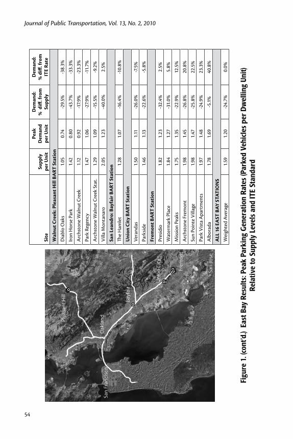
Journal of Public Transportation, Vol. 13, No. 2, 2010
54
Site
Supp
ly
per U
nit
Peak
D
eman
d pe
r Uni
t
Dem
and:
%
diff
. fro
m
Supp
ly
Dem
and:
%
diff
. fro
m
ITE
Rate
Wal
nut C
reek
: Ple
asan
t Hill
BA
RT S
tati
on
Dia
blo
Oak
s
1.
050.
74-29.5%
-38.3%
Iron
Hor
se P
ark
1.
420.
80-43.7%
-33.3%
Arc
hsto
ne W
alnu
t Cre
ek
1.12
0.92
-17.9%
-23.3%
Park
Reg
ency
1.47
1.06
-27.9%
-11.7%
Arc
hsto
ne W
alnu
t Cre
ek S
tat.
1.29
1.09
-15.5%
-9.2%
Vill
a M
onta
naro
2.
051.
23-40.0%
2.5%
San
Lean
dro:
Bay
fair
BA
RT S
tati
on
The
Ham
let
1.28
1.07
-16.4%
-10.8%
Uni
on C
ity
BART
Sta
tion
Vera
ndas
1.50
1.11
-26.0%
-7.5%
Park
side
1.
461.
13-22.6%
-5.8%
Frem
ont B
ART
Sta
tion
Pres
idio
1.82
1.23
-32.4%
2.5%
Wat
erm
ark
Plac
e
1.84
1.27
-31.0%
5.8%
Mis
sion
Peak
s
1.75
1.35
-22.9%
12.5%
Arc
hsto
ne F
rem
ont
1.98
1.45
-26.8%
20.8%
Sun
Poin
te V
illag
e
1.
981.
47-25.8%
22.5%
Park
Vist
a A
part
men
ts
1.97
1.48
-24.9%
23.3%
Alb
orad
a
1.78
1.69
-5.1%
40.8%
ALL
16
EAST
BAY
STA
TIO
NS
Wei
ghte
d A
vera
ge1.
591.
20-24.7%
0.0%
Fi
gure
1. (
cont
’d.)
Eas
t Bay
Res
ults
: Pea
k Pa
rkin
g G
ener
atio
n R
ates
(Par
ked
Vehi
cles
per
Dw
ellin
g U
nit)
R
elat
ive
to S
uppl
y Le
vels
and
ITE
Stan
dard

55
Are Suburban TODs Over-Parked?
In the East Bay, owning and parking a car seemed to be a bit more of a necessity for TOD residents. None of the surveyed East Bay lots was saturated, with, on average, around 25 percent of stalls empty; however, this occupancy rate was higher than in Metro Portland. The weighted average parking rate of 1.2 for East Bay sites matched ITE’s standard, though with a fair amount of variation. At three of the four East Bay stations, nearby parking demand was considerably less than the ITE rate. Below-rate parking levels characterized most projects near the Pleasant Hill BART station, one of the East Bay’s first “transit villages” (Bernick and Cervero 1997). The Fremont BART station is an outlier, inflating the East Bay average. For all projects near Freemont BART, parking levels exceeded the ITE rate, by as much as 41 percent.
In general, overestimation of parking demand suggests people are shedding cars, taking advantage of the accessibility benefits of living near high-quality transit. Fewer cars per household should translate to fewer parked cars. Little is known about car ownership levels for the surveyed projects however some insights can be gained from modal split statistics. In the East Bay, a 2003 survey of residents living in the Verandas Apartments near Union City BART and Park Regency near Pleasant BART found that 54 percent and 37 percent, respectively, commuted to work by transit (versusa2000censusfigureof10.6%ofcommutersinthenine-countySanFranciscoBay Area) (Lund et al. 2004). These high transit mode splits were matched by our findings of relatively low parking demand: 8 percent and 12 percent below the ITE rate for Verandas and Park Regency, respectively. While none of the Metro Portland projects in our sample have been surveyed for modal splits, one study estimated the share of commute trips by transit among those living within ½ mile of the Elmonica and Orenco MAX Stations at 30 percent and 24 percent, respectively (versus a 2000 censustransitcommuteshareof6.4%)(Dill2006).Oursurveysfoundpeak-parkingdemands considerably below ITE rates for both stations (see Figure 1).
While car-shedding no doubt occurs among those living near transit, it might not be as extensive as assumed, particularly among those living in car-dependent suburbs. This is suggested by comparing the differentials between parking genera-tion rates and vehicle-trip generation rates relative to their respective ITE manu-als. A recent study of five TOD housing projects in the East Bay and five in Metro Portland found clear evidence of “trip de-generation”: the weighted average of vehicle trip rates were 40 percent and 27 percent below that estimated by ITE trip generation rates (Cervero and Arrington 2008). As shown in Figure 1, the weighted differential for parking generation matched the ITE rate for East Bay projects and was 11 percent below for Metro Portland projects. Owning and parking a car was particularly a necessity for Fremont’s TOD residents.

Journal of Public Transportation, Vol. 13, No. 2, 2010
56
What’s going on? It is likely that in most suburban TODs, which characterizes the 31 projects in our survey, residents still need access to a car. They just do not use them as much to get to work. But like most suburbanites, they still need a car to get to most non-work destinations, the vast majority of which are away from rail stops. While transit-oriented housing might mean that more trip origins are near rail stops, as long as most destinations are not, many TOD residents still will own cars and use them for shopping , going out to eat, and the like. One policy response to this finding, discussed in the conclusion, is to create car-sharing programs in rail-served neighborhoods. Car-sharing would enable residents not only to rail-commute but also to shed one or more cars.
Why Do Rates Vary?To probe factors that might explain why peak parking demand varies among transit-oriented housing projects, this section presents several best-fitting mul-tiple regression equations. The influences of both on-site and off-site factors on parking demand are investigated. Among on-site factors considered as possible predictors were parking supplies, project size (e.g., land acreage), project density (e.g., land coverage percentages, dwelling units per acre), project design (e.g., whether a gated project, whether surface or structured parking), distance to the region’s CBD, and average rents (a proxy for tenant income levels). A longer list of off-site candidate variables was also considered for model entry, including walk-ing distance, a circuitry index, transit service levels (e.g., headways), road designs (e.g., road widths and presence of nearby freeway interchange), and a number of variables denoting neighborhood attributes within ½ mile of stations, including housing density, income levels, and the presence of retail shops. This analysis thus draws from a substantial literature that holds that various built-environment factors, such as urban densities and walking quality, have a significant bearing on travel behavior (Ewing and Cervero 2001; Handy 2005).
Table 2 presents the best-fitting multiple regression equation for predicting peak parking demand that yielded results consistent with theory and expectations. The two most significant on-site factors—parking supply and project land area—were strongly associated with increased parking demand. These two factors probably are not independent since more spacious land area allows for more parking supply and, in general, a more car-oriented built environment (e.g., wider internal roads). Holding other factors constant, the model estimates that reducing parking by 0.5 spaces per unit will lower peak demand by 0.11 parked cars per unit.

57
Are Suburban TODs Over-Parked?
Table 2. Best-Fitting Multiple Regression Equation for Predicting Peak Parking Rates
Dependent Variable:Peak Parking per Dwelling Unit
Coeff. Std. Err. t Statistic Prob.
Parking Supply: Parking spaces per dwelling unit 0.225 0.122 1.84 .077
Land Area: Project’s land acreage 0.001 0.006 2.254 .033
Walking Distance: Shortest distance along sidewalk network from project center to station, in 1000 ft
0.689 0.307 2.223 .035
Peak Rail Headways: Minutes between trains in AM peak at nearest station
0.059 0.019 3.111 .005
Metro Portland Project: 1 = yes; 0 = no -0.182 0.078 -2.341 .028
Constant 0.122 0.199 0.615 .544
Summary Statistics:F statistics (prob.) = 10.657 (.000)R Square = .681Number of Cases = 31
Among off-site factors, the only two candidates that yielded statistically significant results were walking distance and peak headways of nearby rail services. The model suggests that for every 1,000 feet of walking distance that a project lies away from a station, peaking parking can be expected to increase by 0.7 cars per dwelling unit, all else being equal. Longer headways, denoting less frequent train services, also seem to be an inducement to car ownership and high peak parking demand. A fifth variable in the equation, “Metro Portland Project,” served as a fixed-effect control, denoting less peak parking demand in Metro Portland vis-à-vis East Bay projects. Fixed-effect factors aim to capture the uniqueness of observations from the same city; thus, the significance of this variable could be capturing Portland’s legacy as a pro-transit, smart-growth setting.
While Table 2 reveals a model with fairly good statistical fits—explaining two-thirds of the variation in peaking parking demand—some variables that we felt might be significant were not. Notably, once controlling for walking distance, the circuity of the walk was not significant. This is consistent with findings from other studies showing that quality of walking environment and micro-design features (e.g., presence of street trees) have relatively little influence on travel behavior among those living within five minutes of a station (Cervero 2001; Lund et al.

Journal of Public Transportation, Vol. 13, No. 2, 2010
58
2004). Other non-significant predictors included project density, rent levels, and socio-demographic characteristics of the surrounding neighborhood.
Figure 2 presents a sensitivity analysis of the two variables over which TOD housing developers have some influence: parking supplies and walking distance to a station. Based on the best-fitting multiple regression equation and using mean values for other predictors (i.e., 8 acres of land surface and 8-minute AM peak headways), the figure plots predicted peak parking demand over a range of parking supply and walking distance data. This plot applies to Metro Portland cases (i.e., the variable “Metro Portland Project” was set at 1); however, the same patterns hold for East Bay projects as well (notably, the Y-intercepts of the sloping lines simply slide up by a value of 0.182). For example, the model predicts that at 1.25 parking spaces per unit (roughly ITE’s recommended rate) at 500 feet walking distance from a station, peak parking demand is slightly above 1 space per dwelling unit. At a generous supply of 1.75 spaces per unit and a quadrupling of distance to 25,000 feet, it shoots up to 2.5 parked cars per dwelling unit. Clearly, supply and distance matter.
Figure 2. Sensitivity Analysis: Influences of Parking Supplies and Walking Distances on Predicted Peaking Parking Demand

59
Are Suburban TODs Over-Parked?
One additional multiple regression equation was estimated to shed light on transit usage among TOD tenants. The dependent variable is off-peak parking demand divided by peak parking demand. A high value denotes that significant shares of tenants are leaving their cars at home during daylight hours and thus presumably commuting by transit—i.e., there are almost as many parked cars in the midday as in the wee hours of the morning. Very low values suggest the obverse: most ten-ants are driving to work or other destinations.
Numerous available variables were used as candidate predictors; however, as shown by the best-fitting equation in Table 3, only two were reasonably sig-nificant: land area and walking distance. The coefficients on both variables are negative, indicating that large, spacious projects far removed from stations were associated with most tenants driving to work—i.e., parking lots tended to empty out during the day.
Table 3. Best-Fitting Multiple Regression Equation for Predicting the Rate of Off-Peak to Peak Parking Demand
Dependent Variable:Off-Peak Parking/Peak Parking
Coeff. Std. Err. t Statistic Prob.
Land Area: Project’s land acreage -0.009 0.003 -2.493 .019
Walking Distance: Shortest distance along sidewalk network from project center to station, in 1000 ft
-0.244 0.000 -1.651 .110
Constant 0.688 0.041 16.766 .000
Summary Statistics:F statistics (prob.) = 6.073 (.006)R Square = .303Number of Cases = 31
Case Studies The previous analysis showed that walking distance and parking supplies were the two most significant predictors of parking generation rates. Several case examples around the Fremont BART Station amplify this point. Projects near the Fremont BART station stand out for their high peak parking rates, ranging from 1.23 to 1.69. Alborada Apartments is notable for having the highest peak parking demand of the entire study. Another site, Archstone Fremont Center, distinguishes itself not because its peak generation is unique (at 1.45, its rate is average for Fremont)
Journal of Public Transportation, Vol. 13, No. 2, 2010
60
but because its off-peak generation is so high. The off-peak parking generation at Archstone was 1.14, the highest of all surveyed projects. That is, almost 80 percent of the cars present in the middle of the night were still there in the middle of the day. Archstone’s high ratio (0.78) of off-peak to peak demand indicates that most residents own cars but are not driving for their daily commute. What neighbor-hood and design features might explain the seemingly high level of car parking and use at the surveyed Fremont projects? Focusing on these two “outlier” cases might shed light on this question.
Fremont Station Area The city of Fremont was designed for the car (Renne 2009a). Despite the presence of pedestrian and bicycle infrastructure, such as audible pedestrian countdown signals, bike lanes, and wide, shaded sidewalks, it is not an inviting place to walk or bike due to its scale and the vast distances that separate activities. The streets immediately adjacent to the Fremont BART station are quite wide, ranging from 80 to 100 feet, and the blocks are 800-2000 feet long. Over half of the surveyed projects in Fremont are more than 13 acres in size. A block away from the Fremont station lies large office and institutional buildings that turn large blank walls to the sidewalk. Retail stores and eateries are few and far between.
Fremont BART’s Archstone and Alborada Projects A comparison of Archstone and Alborada reveals several salient differences that could explain variations in parking demand. One difference pertains to on-site uses. Ground-floor retail uses at Archstone (a coffee shop, grocery store, and res-taurants) enable residents to meet basic daily needs on foot en route to or from the BART station. In contrast, Alborada has no retail on-site or along the walkway to BART. This could partly explain why larger shares of Archstone residents leave their cars at home during the workday—i.e., its relatively high off-peak to peak parking ratio.
Another difference pertains to site design. Both Archstone and Alborada are rela-tively large complexes, with 323 and 442 units, respectively, but the projects have strikingly different physical forms (Photo 1). Alborada is a garden-style project with individual buildings interlaced by surface parking. It is an insular, gated develop-ment, set back from the street and detached from its surroundings. Over 16 acres in size, it averages 27 units per acre. Two-thirds of Alborada’s land area is devoted to surface parking and roadways. In contrast, at 54 units and covering only 6 acres, Archstone is more compact, conveying the feeling of an urban place. Cars have
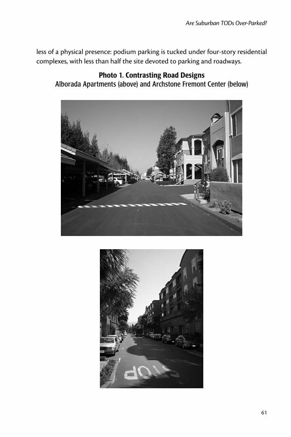
61
Are Suburban TODs Over-Parked?
less of a physical presence: podium parking is tucked under four-story residential complexes, with less than half the site devoted to parking and roadways.
Photo 1. Contrasting Road Designs Alborada Apartments (above) and Archstone Fremont Center (below)

Journal of Public Transportation, Vol. 13, No. 2, 2010
62
It is not form alone but also how Alborado’s design affects connectivity to BART that likely influences travel choices. Despite Alborada lying within a half mile of BART, the shortest walking route to the station is over a mile (Photo 2). This circu-ity results from two factors: (1) the entire perimeter of Alborada’s16-acre expanse is fenced and the sole gate is at the opposite end from the station; and 2) the sheer size of the development, together with limited access points, inflates walking times to almost anywhere. It takes around six minutes to walk from one end of the Alborada complex to the other. Even Alborada residents who take transit may be tempted to drive to the station when faced with a choice of a two-minute drive or a circuitous 20-minute walk along a route lacking anything of pedestrian interest. The fact that reaching the local BART station is far more convenient by car than foot likely contributes to Alborada’s high peak parking rate.
Photo 2. Trip Circuitry Comparison of shortest walking path to straight-line distance from center of
Alborada Apartments project to the Fremont BART station entrance.

63
Are Suburban TODs Over-Parked?
In contrast, Archstone Fremont’s considerably higher off-peak/peak parking ratio is no doubt partly due to easier foot access. Most Archstone tenants are within 10 minutes of the BART fare gate. This is due partially to the fact that Archstone is closer to BART than Alborada, which, as shown earlier in Table 3, is a significant predictor of this ratio. Additionally, Archstone’s proximity is enhanced by the absence of clear borders and fences. The project’s smaller scale and grid layout also create a more pedestrian-friendly setting.
In sum, the Archstone and Alborada cases suggest that the presence or absence of mixed uses, direct pathways, and connectedness to surroundings could very well affect how TOD residents use and park their cars. The Quatama MAX station in Beaverton, Oregon , can serve as a model for cities such as Fremont on designing for transit connectivity. There, a walking path provides direct and nicely-landscaped access to the MAX station (Photo 3). The city required the project developer to build the path as a condition of approval. Retrofitting current development with such pathways, while challenging, could improve current pedestrian connectivity, and requiring such pathways in new developments could ensure better connectiv-ity in the future.
Photo 3. Pathway from the Quatama Station toward nearby residences
Journal of Public Transportation, Vol. 13, No. 2, 2010
64
TOD Parking OrdinancesWhile our research has found that peak parking levels of housing near suburban rail stops are not significantly below national averages (based on ITE data), we also found that factors such as constrained parking supplies and short walking distances to stations can lower demand. In light of these findings, have cities been responsive through their parking zoning ordinances, making adjustments for proj-ects near rail transit?
National SurveyTo probe this question, we conducted a national survey. The sample frame was all U.S. cities with rail transit stations, identified using coordinates from the Center for Transit-Oriented Development station database. From this list of cities, contact information was gathered and an online survey was sent to senior planning staff.
Of the 363 cities surveyed, 22 percent (or 80 in total) returned a completed ques-tionnaire, which is in line with typical response rates for online surveys (Fink 2003). A higher response rate of 40 percent from cities with over 100,000 residents and a 10 percent response rate from cities under 10,000 skewed the sample to an aver-age population of 167,000 versus 144,000 for all cities with rail stops. Ten or more responses were received from cities in metropolitan Los Angeles, San Francisco-Oakland, Chicago, and the Washington-Boston corridor.
Survey FindingsOf thecities surveyed,nearly all (96%)have some formofminimumoff-streetparking requirement for multi-family housing. Most cities with minimum parking requirements (89%)alsoallow forvariancesor exceptions to theseminimums.Proximity to rail transit is grounds for a variance in 39 percent of cities that allow variances, which is just over one third of all cities with minimum off-street parking requirements for multi-family housing. Parking space reductions for proximity to rail transit range from fewer than 10 percent to as high as 60 percent, with a mean reductionof22.8percent(standarddeviation=13.7%).
Differences by housing type and across locations in a city complicate the ability to quantify a city’s average or typical parking requirement. In the interest of obtain-ing some sort of comparison, we calculated per-unit parking requirements in each city for a hypothetical transit-oriented multi-family housing project located ¼ mile from a rail station using zoning requirement and variance information that was provided. These calculated minimum off-street parking requirements are, of

65
Are Suburban TODs Over-Parked?
course, a simplification and likely miss some nuances of applied zoning codes, but they provide a useful tool for comparing requirements across jurisdictions.
The calculated off-street minimum parking requirements for transit-oriented multi-family housing in our sample ranged from 0 to 3 parking spaces per unit for both one and two bedrooms units. The mean across all cities surveyed was 1.37 stalls per one-bedroom unit and 1.61 per two-bedroom unit, both above the ITE per-unit rate of 1.2. If we assume an even mix of one- and two-bedroom units, our average calculated parking requirement for a hypothetical transit-oriented hous-ing project is 1.48 per unit, well above the ITE average of 1.2 per unit and even above ITE’s 85th percentile of 1.46 per unit. Put another way, 75 percent of cities surveyed have minimum TOD parking requirements that exceed ITE parking gen-eration rates. Based on both ITE rates and the empirical findings presented earlier, these numbers show that even when cities adjust parking requirements to take transit-proximity into account, far too much parking is required.
Respondents also were asked questions about their views on current parking poli-cies and the willingness of elected officials and developers to support changes to parking requirements. When asked about their city’s current minimum off-street parking requirements near rail stops, 59 percent of respondents answered they “are about right”; however, 37 percent replied “too much was being required.” When asked about the likely stance of local elected officials to lowering minimum off-street parking requirements for multi-family housing near rail transit, 59 per-cent of those who responded felt officials would be supportive versus 32 percent who thought they would be opposed. Moreover, among those who recorded a response, 85 percent felt elected officials would oppose efforts to eliminate minimum parking requirements even if a project is near a rail stop. However, 55 percent also believed elected officials would support efforts to set a cap on parking for housing near rail transit.
In general, survey respondents felt housing developers were inclined to provide less parking than necessary. Among those answering the question, 60 percent felt that developers of multi-family housing would build too little parking if given the chance. Just 10 percent felt developers would provide too much parking. The prevalence of high minimum parking requirements likely reflects the public sec-tor’s fear that, if left to their own accord, private developers will under-supply parking. Planners fear the resulting spillover will affect surrounding neighbor-hoods, which was cited by respondents as the number one obstacle to enacting zoning reforms.

Journal of Public Transportation, Vol. 13, No. 2, 2010
66
Conclusions This study posed the question: “Are TODs over-parked?” From a design standard perspective, our response is “probably so.” For the 31 surveyed multi-family proj-ects combined, there were 1.57 spaces per dwelling unit, nearly one third higher than ITE’s suburban standard of 1.2 spaces per unit. From a supply-demand stand-point, transit-oriented housing also seems over-parked: the weighted-average sup-ply of 1.57 spaces per unit was 37 percent higher than the weighted-average peak demand of 1.15 parked cars per unit. From our national survey responses, there is evidence of over-parking: the estimated average minimum parking requirement for multi-family housing near rail transit was 1.48 spaces per unit, also well above the ITE standard. From a pure demand standpoint, however, it appears that peak parking demand for transit-oriented housing aligns fairly closely with the ITE stan-dard. Experiences in the East Bay and Metro Portland suggest that TODs are only slightly over-parked, if at all. In sum, we believe parking supplies are over-inflated, not due to bloated ITE design standards but other factors, such as developers’ fears of insufficient parking to attract prospective tenants or local officials’ fears of spillover on-street parking problems in surrounding neighborhoods. It is because of such concerns that municipal parking standards for TOD housing appear on the high side, which probably further induces car ownership and usage—i.e., the classical vicious cycle of supply and demand feeding off each other.
We acknowledge that a simple comparative analysis such as ours has limita-tions and is certainly not the final word on this subject. For this reason, we have refrained from using words such as “caused” or “proved” in describing relation-ships. The best we can say is that many suburban TODs appear to have more park-ing than is needed. In truth, “thumbs-up/thumbs-down” decisions on whether to approve proposed TOD projects rely heavily on the kinds of simple comparisons to ITE rates presented in this paper. They certainly are not based on multinomial logit estimates of transit ridership impacts. While we, no doubt, need more sophis-ticated studies that probe the influences of parking supplies and policies on travel behavior and car ownership, there is also a need for straightforward comparisons of actual and estimated rates to inform TOD design and approval decisions.
While we conclude that transit-oriented housing seems to be mostly over-parked, the research also points to factors that can moderate demand. As expected, supply matters. From our regression estimates, reducing parking by 0.5 spaces per unit is associated with 0.11 fewer cars parked per unit at the peak. Also, parking demand generally fell as the walking distance to a station shortened. Smaller scale projects
67
Are Suburban TODs Over-Parked?
with less land coverage also average lower parking rates. These findings favor clus-tered development with good internal pathways that provide fairly short, direct connections to rail stops. Such designs can shrink parking demand and its foot-print, unleashing a “virtuous cycle”—i.e., less land is given over to surface parking which, in turn, allows more compact site designs. Last, the other policy lever to lower parking demand is transit service levels. Our model showed that reducing headways between trains reduces parking loads, ostensibly because one is less in need of a car in areas with superb transit services.
Other policy responses also are supported by our findings. One response should be the introduction of more flexibility in parking policies for housing near rail stops. Flexibility can be in the form of enabling projects to provide below-code parking levels when justified—e.g., compact projects with short, direct walking connections to transit and perhaps on-site retail establishments. In their chapter “Ten Principles for Developing around Transit,” Dunphy et al. (2004, p. 174) note that “flexible parking standards provide some latitude in providing the optimal number of parking spaces.” Flexibility also can take the form of unbundling the cost of providing parking from the cost of building (or renting) housing (Daisa 2004; Shoup 2005). This would allow developers to better scale the amount of parking provided to what each tenant or homeowner is willing to pay for each car owned—i.e., let the market demand, rather than a possibly outdated govern-ment fiat, determine supply. And flexibility can be in the form of allowing TOD tenants to choose deeply discounted transit passes for frequent riders instead of a 300 square foot parking space. Shoup (2005 p. 259) argues that the substitution of such “Eco Passes” for parking among transit-oriented residents could “reduce the cost of TOD, improve urban design, reduce the need for variances, and reduce traffic congestion, air pollution, and energy consumption … at a low cost.”
Our finding that TODs de-generate automobile trips a lot more than they de-generate parking demand, at least relative to ITE standards, suggests TOD resi-dents commute by transit proportionately more than they shed cars. That is, many self-select into TOD neighborhoods for the very reason that they want to avoid congestion and thus take transit to work, but for non-work travel, they still need a car. We believe a significant share of TOD residents would shed a car if they had carsharing options. Cervero et al. (2007) carried out a panel study of how San Fran-cisco’s City CarShare program affected car ownership. Four years after the inaugu-ration of City CarShare, 29 percent of carshare members had gotten rid of one or more of their cars, and 63 percent lived in zero-vehicle households. A predictive

Journal of Public Transportation, Vol. 13, No. 2, 2010
68
model showed that living close to a carshare pick-up spot was strongly associ-ated with car-shedding. By extension, putting shared-cars in and around TODs could relieve many households from owning a second car or a vehicle altogether. Through a combination of proximity advantages and lifestyle predispositions, liv-ing near transit can de-generate vehicle trips. And with the option of car-sharing, it can likely reduce parking demands as well.
References
Bernick, M., and R. Cervero. 1997. Transit Villages for the 21st Century. New York: McGraw-Hill.
Boarnet, M., and R. Crane. 2001. Travel by Design: The Influences of Urban Form on Travel. New York, Oxford University Press.
Cervero, R. 1994. Transit-based housing in California: Evidence on ridership impacts. Transport Policy 1(3): 174-183.
Cervero, R. 2001. Walk-and-ride: Factors influencing pedestrian access to transit. Journal of Public Transportation 3(4): 1-23.
Cervero, R., and others. 2004. Transit Oriented Development in America: Experi-ences, Challenges, and Prospects. Washington, D.C.: Transit Cooperative Research Program, Report, 102.
Cervero, R. 2007. Transit oriented development’s ridership nonus: A product of self selection and public policies. Environment and Planning A 39: 2068-2085.
Cervero, R., A. Golub, and B. Nee. 2007. City CarShare: Longer-term travel-demand and car ownership impacts. Transportation Research Record 199: 70-80.
Cervero, R., and G. Arrington. 2008. Vehicle Trip Reduction Impacts of Transit-Oriented Housing. Journal of Public Transportation, 11 (3): 1-17.
Daisa, J. 2004. Traffic, parking, and transit oriented development. In Dittmar, H., and G. Ohland, eds. The New Transit Town: Best Practices in Transit-Oriented Development. Washington, DC: Island Press, pp. 114-129.
Dill, J. 2006. Travel and Transit Use at Portland Area Transit-Oriented Develop-ments (TODs). Seattle: Final Technical Report, Transportation Northwest (TransNow).
69
Are Suburban TODs Over-Parked?
Dunphy, R. 2004. Who, What, Where, Why. In DunphyR., et al., eds. Developing Around Transit: Strategies and Solutions That Work. Washington, D.C.: Urban Land Institute, Chapter One.
Dunphy, R., D. Myerson, and M. Pawlukiewicz. 2004. Ten Principles for Developing Around Transit. In Dunphy, R., et al., eds., Developing Around Transit: Strate-gies and Solutions That Work. Washington, D.C.: Urban Land Institute, Chapter Seven.
Ewing, R., and R. Cervero. 2001. Travel and the built environment: A synthesis. Transportation Research Record 1780: 87-114.
Fink, A. 2003. The Survey Kit. Thousand Oaks, California: Sage Publications.
Handy, S. 2005. Smart Growth and the transportation-land use connection: What does the research tell us? International Regional Science Review 28(2): 1-22.
Hess, D., and P. Lombardi. 2004. Policy support for and barriers to transit-oriented development in the inner city: Literature review. Transportation Research Record 1887: 26-33.
Institute of Transportation Engineers. 2003. Parking Generation. Washington: ITE, 3rd Edition.
Karp, J. 2008. Suburbs a mile too far for some. Wall Street Journal, June 17, 2008, A18.
Loukaitou-Sideris, A., and T. Banjaree. 2000. The blue line blues: Why the vision of transit village may not materialize despite impressive growth in transit rider-ship. Journal of Urban Design 5(2): 101-125.
Lund, H., R. Willson, and R. Cervero. 2006. A re-evaluation of travel behavior in Cali-fornia TODs. Journal of Architecture and Planning Research 23(3): 247-263.
Poticha, S., and J. Wood. 2008. Transit oriented for all: Delivering mixed-income housing in transit served neighbourhoods. In Curtis, C., et al., eds., Transpor-tation Oriented Development: Making It Happen. Surrey, England: Ashgate, 153-169.
Renne, J. 2009a. From transit-adjacent to transit-oriented development. Local Environment 14(1): 1-15.

Journal of Public Transportation, Vol. 13, No. 2, 2010
70
Renne, J. 2009b. Measuring the success of transit oriented development. In Curtis, C., et al., eds., Transportation Oriented Development: Making It Happen. Surrey, England: Ashgate, pp. 241-255.
Shoup, D. 2003. Truth in transportation planning. Journal of Transportation and Statistics 6: 1-16.
Shoup, D. 2005. The High Cost of Free Parking. Chicago: Planner’s Press.
Urban Land Institute. 2004. Emerging Real Estate Markets: 2004. Washington: ULI.
Willson, R. 2000. Reading Between the regulations: Parking requirements, planners’ perspectives, and transit. Journal of Public Transportation 3(1): 111-128.
About the Authors
Robert Cervero ([email protected]) is professor of City and Regional Plan-ning at the University of California, Berkeley, where he also directs the Institute of Urban and Regional Development and the University of California Transportation Center (UCTC).
Arlie Adkins ([email protected]) is a recent graduate in City Planning at the University of California, Berkeley and is currently enrolled in the doctoral program in Urban Studies at Portland State University. He previously worked as a transit planner with Portland’s TriMet.
Cathleen Sullivan ([email protected]) just completed a Masters in City Planning at the University of California, Berkeley. She now works as a trans-portation planner for Nelson\Nygaard Consulting Associates in San Francisco.

Effect of Variable Bus Speeds on Bus Network Design
71
Effect of Variable Bus Speeds on Bus Network Design
Nicole Foletta, Miquel Estrada, Mireia Roca-Riu, and Pere Martí Center for Innovation in Transport (CENIT)
Abstract
This article provides a methodology for solving the bus network design problem, covering network design and frequency setting and taking into consideration that commercial speeds of buses vary depending on the aggregated frequency of buses on each corridor. This methodology, referred to as Variable Speed Methodology, uses a variation of an algorithm proposed by Baaj and Mahmassani that assumes speeds remain constant (denoted Fixed Speed Methodology). Both methodologies were applied to the street network of Barcelona. Outputs were compared, and it was found that the Variable Speed Methodology produces a bus network with faster average travel speeds, shorter travel times, smaller fleet size, less route kilometer, and fewer buses per link while still serving the same level of demand. These results demonstrate that taking variability of bus speeds into consideration when performing route gen-eration and frequency setting can significantly improve the performance of the bus network produced.
IntroductionThe focus of this article is the analysis of the bus network design problem. Planning an efficient transit network is a complex process and usually is divided into three main components: strategic planning (network design), tactical planning (fre-quency setting) and operational planning (allocation of resources to each route). Through re-evaluation of both network layout and route frequency setting, great

Journal of Public Transportation, Vol. 13, No. 2, 2010
72
improvements in the efficiency of a transit network are possible, and both user and operator costs can be reduced. This is particularly important as public trans-portation systems have become an integral and essential tool for cities to tackle the problems of escalating vehicle emissions and congestion.
It is notable that in several cities, such as Barcelona, a common practice of public transportation planners has been the concentration of several key bus routes along the main corridors of the city. This measure strengthens the ease and number of transfers at shared stops along the corridor, although as number of buses increases, the aggregated bus flow may approach the theoretical capacity value of the lane or bus stop. The key consequences of this effect are queues of vehicles at stops and a significant drop in the commercial speed of buses. It is important to take such factors into consideration when creating or expanding a transit network.
Previous research on route generation and frequency setting has not taken con-gestion into consideration. The main objective of this article is to provide a meth-odology for the network design problem that covers both strategic planning and tactical planning, taking into consideration that commercial speeds of buses vary depending on the aggregated flow of buses on each corridor. Its main application is in areas with high bus frequency, as is the case in many cities in South America and Europe. The aim of the methodology is to generate a set of routes and fre-quencies that minimize both user and operator costs.
This article is organized as follows. The following section summarizes past research on this topic, and then the methodology is described. Next, the methodology is applied to Barcelona’s street network, and experimental results are detailed. The most important conclusions of the work are summarized, information for apply-ing the model is provided, and steps for future research are briefly discussed.
BackgroundMuch attention has been paid to the bus network design problem and the setting of efficient frequencies to cover demand. The problem is considered NP-complete and, therefore, a way to find an optimal solution can take a considerable amount of time, especially for large problems (Van Ness 2002). For this reason, most research related to this topic has included adding constraints to the problem or reducing the search space in order to shorten calculation time within reasonable limits. However, the resulting solutions may not be optimal.
Effect of Variable Bus Speeds on Bus Network Design
73
In past research, two approaches generally have been used for transit route gener-ation: a continuous approach and a discrete approach. The continuous approach formulates a problem on a solution space with certain completeness. In general, this approach provides a global optimal solution, but the solution might not be realistic. For example, the solution might contain stop spacing or line spacing that is not applicable on the actual network (Van Ness and Bovy 2000). This approach works well for small problems, but as the size of the problem increases, solution time quickly reaches unreasonable values.
The discrete approach formulates the problem directly on possible solution sub-spaces defined based on domain specified heuristic guidelines. This approach will provide a feasible solution, but often not a global or even local optimal solution. However, the discrete solution generally requires much less computing time, dem-onstrating the tradeoff between solution optimality and computational time.
Recently, the development of algorithms based on local search and metaheuristics have been implemented in the bus network design problem in order to further optimize the network produced (Chien et al. 2001; Ngamchai and Lovell 2003; Verma and Dhingra 2005). Finally, other metaheuristics such as taboo search or simulated annealing have been used to search the optimal set of routes in the solu-tion domain (Fan and Machemehl 2006).
Table 1 provides a summary of past research on this topic, including both the continuous and discrete approaches. The objective of each of these models is to produce a set of bus routes and route frequencies.

Journal of Public Transportation, Vol. 13, No. 2, 2010
74
Table 1. Overview of Past Research on Transit Network Design
Author Description
Lampkin and Saalmans (1967) Minimize travel time given fleet size and vehicle size.
Hasselstrom (1981) Maximize number of passengers (demand) given budget and minimum frequency constraints.
Ceder and Wilson (1986) Minimize travel time, transfer time and fleet size given con-straints on route length, number of routes and frequency.
Janarthanan and Schneider (1988)
Includes manual network design, assignment and feedback.
Van Nes et al. (1988) Maximize the number of passengers with no transfer given a budget constraint.
Baaj and Mahmassani (1995) Includes computer aided network design, assignment and line improvement.
Ceder and Israeli (1998) Minimize travel time, empty seat hours and fleet size.
Shih et al. (1998) Includes computer aided network design, transfer nodes, assignment and line improvement.
Chien et al. (2001) Minimize user and supplier costs subject to constraints, ap-plies genetic algorithm.
Saka (2001) Reduce operating costs by finding optimal spacing of buses.
Ngamchai and Lovell (2003) Includes frequency setting and headway coordination. Ap-plies a genetic algorithm to help optimize bus transit route design.
Verma and Dhingra (2005) Routes are generated based on shortest paths, also considers transfers to rail stations. Applies a genetic algorithm.
Fan and Machemehl (2006) Includes computer aided network design and assignment. Applies a simulated annealing procedure to select an opti-mal set of routes.
MethodologyThe aim of the methodology proposed in this article is to solve the bus network design problem and frequency determination. This methodology includes a modi-fication of the solution approach proposed in Baaj and Mahmassani (1995). While the contribution of Baaj and Mahmassani assumes that the shortest path between nodes remains fixed, our methodology recalculates the shortest path during the network building process. This information subsequently is used to determine frequencies and develop the assignment of passengers to the network. The overall methodology process is outlined in Figure 1. On the right is the methodology pro-posed in Baaj and Mahmassani (1995), referred to here as the Fixed Speed Meth-odology (FSM), and on the left is the new methodology proposed in this article,

Effect of Variable Bus Speeds on Bus Network Design
75
referred to as the Variable Speed Methodology (VSM). Both consist of two princi-pal components: (1) the route generation algorithm (RGA) which designs routes, and (2) the assignment process, which assigns demand to the network, determines frequencies, and evaluates network performance. In the following subsections, the Variable Speed Methodology is described as are the differences between it and the Fixed Speed Methodology.
Figure 1. Model Methodology

Journal of Public Transportation, Vol. 13, No. 2, 2010
76
Methodology Inputs and FormulationBoth methodologies require information about the underlying street configura-tion on which the bus network will be created, the demand distribution in the network and the minimum performance quality required. We represent the street configuration by a directed graph G=(N,L), with node set N representing transit stops and intersections and link set L representing links between nodes. We denote d as an asymmetrical bus demand matrix, where the element dij represents the demand between node i and node j. Regarding quality of service, a number of parameters are set by the user, including the minimum percentage of demand that must be satisfied by the bus network.
The solution of these methodologies is the bus network and its frequencies. The bus network can be described as a set of routes, R={r1,r2,r3,...,rs}, where each route, rz, is defined by a sequence of nodes: rz={(i,j),(j,k),..,(u,v)}/ i,j,k,u,vN. Each route, rz, has a scheduled frequency, fz (bus/h).
Route GenerationThe route generation algorithm (RGA) is a heuristic algorithm for route design. Its three main features are (1) it is heavily guided by the demand matrix, (2) it allows the designer’s knowledge to be implemented so as to reduce the search space, and (3) it generates different sets of routes corresponding to different trade-offs among conflicting objectives. The algorithm starts by creating a number of initial skeletons (M) for the routes, which are expanded and complemented as demand is assigned to existing or new route segments. At the end of the process, a minimum percentage of total demand must be satisfied directly with zero transfers (D0), and a minimum percentage of total demand with one or fewer transfers (D1).
Modified Route Generation Algorithm. The RGA described in Baaj and Mahmas-sani (1995) was modified to include additional features. The main difference is that the Modified RGA (MRGA) recalculates travel times on links in order to account for reduced speeds due to bus congestion (particularly related to interference at bus stops). In addition, the MRGA accommodates networks with one-way streets by designing both an initial route and a return route. The structure of the MRGA consists of the following steps.
Select the node pair (1. i,j) with the highest demand not yet satisfied and search for the shortest path between the nodes.
Expand the path generating a new route.2.
Design the return route. 3.

Effect of Variable Bus Speeds on Bus Network Design
77
Filter the set of routes: check if any routes are overlapped, if there is an 4. overlap delete the smallest route.
Re-calculate new travel times on the links with congestion.5.
Add new route to set of routes and compute the directly served demand. If 6. it is greater than D0 go to the next step; otherwise, go to step 1.
Compute the demand served with zero or one transfer. If it is greater than 7. D1, stop and return the set of routes; otherwise, go to step 1.
Travel Time Calculation. A key variation between the FSM and VSM is the con-sideration that bus travel speeds will vary based on the flow of buses in the lane. This variation will affect the travel times calculated on each link. The FSM assumes that travel speeds are constant no matter how many buses are using the link. How-ever, the Transit Capacity and Quality of Service Manual (TCQSM) by Kittleson & Associates et al. (2003) presents an analysis of bus speeds, providing a compact formula to estimate this operational variable. Equation 1 is taken from this report and evaluates bus commercial speeds as a function of a basic travel time, time spent at intersections, the effect of skip-stop operations, and the effect of interfer-ence from other vehicles.
(1)
Where:
St : Speed on link t
tr : Basic travel time considering dwell time
tl : Time spent at intersections considering effects of other vehicles
fs : Parameter measuring the effect of skip-stop operations
fb : Parameter measuring the effect of interference from other buses
The basic travel time, tr , is determined by taking an estimate of bus running times as a function of stop spacing and average dwell time per stop. Running time losses, tl , are estimated considering effects of traffic signals, intersections, and other vehicles sharing the lane. TCQSM contains estimated values for these variables (based on field measurements) considering five different lane configurations: (1) bus lane, (2) bus lane with no right turns, (3) bus lane with right turn delays, (4) bus lane blocked by traffic, and (5) mixed traffic flow.

Journal of Public Transportation, Vol. 13, No. 2, 2010
78
Our modification does not consider the effect of skip-stop patterns ( fs is equal to one). However, the parameter fb is especially important because it is ruled by the relationship between bus flow and lane capacity. As the flow of buses in the lane increases, the probability of buses having to wait for other buses at bus stops or buses needing to pass other buses increases, thus reducing the overall speed of buses. Table 2 displays the values used for fb , as evaluated in TCQSM. This param-eter is the key behind our measurement of the variation of bus speeds.
Table 2. Values for Bus-Bus Interface Factor
Lane Volume/Capacity Ratio Bus-Bus Interface Factor (fb)
<0.5 1.00 0.5 0.97 0.6 0.94 0.7 0.89 0.8 0.81 0.9 0.69 1.0 0.52 1.1 0.35
The travel time on each link is calculated by taking the length of the link divided by the speed on the link (St ). In the VSM, link travel times are recalculated after each route is generated using the speed of Equation 1. If the new route shares a link with an existing route, the parameter fb could be affected, thus changing the values of the link speed and link travel time. The link travel times are used to calculate the shortest path between each node pair. Therefore, the adjusted link travel times are used when determining each subsequent route.
One important consideration is that the travel times on each route generated by the FSM will appear lower than would be evaluated in a real network with high transit frequencies. Therefore, after the routes have been generated for the FSM, the speed on each link is recalculated, using Equation 1, to account for the effect of multiple buses on a link.
Network AssignmentNetwork assignment is the process of assigning demand to the bus network. Once routes have been generated by RGA and MRGA, the network assignment process is applied to the routes to determine frequencies and generate a set of performance indicators. The network assignment process used in the models is a program called TRUST, described in Baaj and Mahmasani (1990). This assignment method uses a transit path choice logic to apply the demand to the network, con-sidering number of transfers as the most important criteria.
Effect of Variable Bus Speeds on Bus Network Design
79
AnalysisThe FSM and VSM were programmed using JAVA. The two models were applied to the street network of Barcelona, which is composed of 5,928 street nodes and 8,783 links. Of the street nodes, 198 are potential bus stops with a total of 12,254 non-zero origin-destination pairs. The average daily demand matrix during the peak hour (8:00 AM - 9:00 AM), with an associated demand of 51,689 passengers per hour, was obtained from data from a mobility survey of the metropolitan area of Barcelona (IDESCAT 2001).
Speed Calculation ValidationAn analysis was performed to assure that the speed calculation shown in Equation 1, defined in TCQSM, was appropriate for the case of Barcelona. The values of tr , tl
and fb were analyzed using real data from the city of Barcelona. The real values were found to be similar to the values detailed in TCQSM in all cases (CENIT 2006).
In particular, data for the bus-bus interface factor ( fb) collected for the city of Barcelona produced the following best-fit curve (Equation 2). These values match very closely with the values from TCQSM, listed in Table 2.
(2)
Where:
fb : Parameter measuring the effect of interference from other buses
v : Lane volume (vehicles/hour)
C : Lane capacity (vehicles/hour)
Subsequently, the TCQSM model for calculating velocity was used to estimate velocity in Barcelona during different periods of the day. These values were com-pared with the actual velocity values of buses in Barcelona during those periods, and the differences were very small, with a maximum error of 15 percent. This analysis validates the TCQSM model as an appropriate model for estimating the velocity of buses in the city of Barcelona. Therefore, values of tr , tl and fb were taken from the corresponding tables in TCQSM.
Parameter InputsAs mentioned, many parameter values must be defined by the user. The param-eters in Table 3 were selected specifically for the case of Barcelona. In addition,

Journal of Public Transportation, Vol. 13, No. 2, 2010
80
the values from Table 2 were used to define fb , which varies based on the flow of buses in the lane.
Table 3. Parameter Values for Barcelona Network
Variable Description Value
M Initial number of skeleton routes 7
D0 %ofdemandthatmustbesatisfiedwith0transfers 20%-80%
D1 %ofdemandthatmustbesatisfiedwith1orfewertransfers 50%-100%
tr Base bus running time (min/km) 3.49
tl Base bus running time losses (min/km) 1.2
Ttran Transfer time penalty (min) 5
Cap Seated bus passenger capacity (passengers/bus) 90
LFmax Maximum allowable load factor 1.25
Several scenarios have been considered regarding various combinations of D0 and D1. These variables greatly influence the composition of the bus network created because the algorithms will continue adding routes to the network until these minimum demand values are satisfied. The value of D0 governs the directness of service, while D1 influences network coverage. Table 4 summarizes the various combinations of D0 and D1 used.
Table 4. Input Values for D0 and D1 D0 (%) D1 (%) 20 50 20 60 20 80 20 90 20 100 40 60 40 80 40 90 40 100 60 80 60 90 60 100 80 90 80 100

Effect of Variable Bus Speeds on Bus Network Design
81
Sensitivity AnalysisThe inputs listed in Table 3 and Table 4 were used for both the VSM and FSM. Figure 2 displays the total travel time in terms of passenger-minutes for each model run versus the percentage of the total demand satisfied by one or fewer transfers (each point represents a different combination of D0 and D1 for each of the models). The slightly larger markers represent the case where D0=40%andD1=60%.Itshouldbenotedthatthedemandsatisfiedbythenetworkmightbehigher than the minimum demand required by D1, since as routes are added to the network, demand satisfied increases in discrete increments. These results show that as demand satisfied increases, total passenger travel time also increases. This is intuitive since as the number of passengers served increases, the total passenger-minutes also increase. The networks created by the VSM satisfy the demand using fewer overall passenger minutes than the networks created by the FSM.
Figure 2. Total Travel Time vs. Satisfied Demand
Figure 3 shows the mean passenger travel time versus satisfied demand. The VSM model provides shorter travel times than the FSM model. This is a very attractive quality for users.

Journal of Public Transportation, Vol. 13, No. 2, 2010
82
Figure 3. Mean Travel Time vs. Satisfied Demand
Figure 4 shows the number of buses versus satisfied demand. This plot shows that as demand satisfied increases, the number of buses required to serve that demand also increases, which is expected. The VSM generally requires fewer buses to serve the same level of demand as the FSM. This suggests that the buses in the VSM networks are used more efficiently.
Figure 5 depicts the percentage of total routes that have low ridership versus the minimum demand satisfied directly. Low ridership routes are defined as those requiring fewer than one bus per hour. As demand satisfied directly increases, per-cent of low ridership routes also increases. Furthermore, when D1=100%,meaningall demand must be satisfied with one or fewer transfers, the percent of low rider-ship routes increases significantly. These results demonstrate that forcing a higher percentage of demand to be satisfied directly or requiring that all demand be satisfied will lead to a higher occurrence of low ridership routes. This reduces the efficiency of the network because more resources are required to provide services on routes that are used by fewer passengers, thus requiring more resources per passenger served. These passengers might be more efficiently served by demand-responsive transit services such as paratransit.

Effect of Variable Bus Speeds on Bus Network Design
83
Figure 4. Fleet Size vs. Satisfied Demand
Figure 5. Percent Low Ridership Routes vs. Demand Satisfied Directly
Figure 6 shows the mean passenger travel speed versus satisfied demand. The mean passenger travel speed does not include waiting time or time stopped at bus stops, but includes only the average time all passengers spend traveling on links in the system. As Figure 6 demonstrates, networks created by VSM have higher passenger travel speeds in networks with less than 95 percent of demand satisfied.

Journal of Public Transportation, Vol. 13, No. 2, 2010
84
However, when demand satisfied reaches 100 percent, the networks designed by both VSM and FSM seem to have similar travel speeds. This could be because, to satisfy a higher percentage of the demand, the network must be extended to cover more nodes, thus creating routes on outlying links and reducing frequencies, hence reducing congestion in the network, which, in turn, increases travel speeds. However, it should be noted that this increase in travel speed comes at the cost of reduced efficiency in the network and higher operating costs.
Figure 6. Mean Passenger Travel Speed vs. Satisfied Demand
Figure 7 shows mean route speed versus mean route frequency. As frequency increases for FSM, route speed decreases dramatically. This is likely a result of sev-eral bus routes running on the same streets, causing bus speeds to decrease as bus congestion and bus interference at stops increases. In the VSM, however, route speed decreases at a slower rate as frequency increases. This suggests that the bus networks generated by VSM are more spread out across the street network and, as a result, encounter less congestion. Even as bus frequencies increase overall, it has a much lower impact on bus speeds.
As discussed, a variety of potential bus networks can be produced depending on the model used and inputs selected. The above analysis shows that VSM generally provides a more efficient network than FSM.

Effect of Variable Bus Speeds on Bus Network Design
85
Figure 7. Mean Passenger Travel Speed vs. Mean Route Frequency
Model Results Using Same InputsTable 5 displays the most important parameters for measuring the performance of the bus networks produced by each of the models when the same set of inputs are entered into each. The values D0=40%andD1=60%wereselectedforthisanalysisbecause the networks produced have reasonable values for each of the indicators analyzed; for example, the percent of demand served is high while the number of low ridership routes and fleet size are relatively low. These networks are denoted in the previous figures by slightly larger markers. The network produced by the VSM serves about the same amount of demand as the FSM. Both serve the minimum amount required plus additional demand due to the discrete addition of routes to the network. The VSM network requires more routes but fewer buses than the FSM network and fewer route kilometers, which would result in lower expenses for purchasing buses and providing bus maintenance.
The mean passenger travel speed is higher for VSM than for FSM. This reflects the importance of variable speed consideration in the network design process. In addition, the VSM network has a lower mean passenger travel time than the FSM network. This signifies that the VSM network is more attractive to passengers than the FSM network.
The maximum number of buses operating on a single link is lower for VSM; fur-thermore, the network produced by VSM has the highest percentage of links in

Journal of Public Transportation, Vol. 13, No. 2, 2010
86
the street network covered by routes. This demonstrates that VSM produces a network that is more spread out, covering more links, and the links in the network are less congested than the network produced by the FSM.
These results are specific to this set of inputs and results can vary depending on the inputs used, but based on this analysis, VSM tends to produce a more efficient network and one that is more attractive to both users and operators than FSM.
Table 5. Comparison of Networks
NETWORK COMPARISON FSM VSM % Difference
Total demand (pax/hr) 51,689 51,689
Demandassigned,D1(%) 60 60
Demandwithnotransfer,D0(%) 40 40
Demand served with 0 transfers (pax/hr) 19,858 19,805 -0.3%
Demand served with 1 transfer (pax/hr) 22,582 21,978 -2.7%
Demandsatisfied(%) 85 84 -1.2%
Number of routes 112 115 2.7%
Percentoflowridershiproutes(%) 12 11 -8.3%
Fleet (vehicles) 861 803 -6.7%
Max buses per link 110 98 -10.9%
Linkscoveredbyroutes(%) 51 53 3.9%
Mean frequency of the routes (buses/hr) 3.5 3.5 0.0%
Mean passenger travel time (min) 57 55 -3.5%
Mean person speed (km/hr) 11.8 12.4 5.1%
Total travel time (pax·min) 2,669,388 2,585,779 -3.1%
Total route kilometer 2,805 2,798 -0.2%
Total seat kilometer offered (pax·km), SKO 908,290 896,633 -1.3%
Total person kilometer transported (pax·km), PKT
462,438 455,045 -1.6%
Load factor (PKT/SKO) 0.51 0.51 0.0%
Bus Network Layout ComparisonThe bus network layout and vehicle flow distribution associated with these two networks are represented in Figures 8 and 9. At first glance, both networks share the corridors with more demand (transversal arterials). Nevertheless, the network
INPU
TSO
UTP
UTS

Effect of Variable Bus Speeds on Bus Network Design
87
proposed by the VSM covers more streets, providing a more extensive network, and, generally, each street has less frequency, therefore reducing congestion. On the other hand, the network proposed by the FSM presents a consolidation of routes on fewer streets, which worsens the bus congestion phenomenon.
Figure 8. Network Layout for FSM
Figure 9. Network Layout for VSM

Journal of Public Transportation, Vol. 13, No. 2, 2010
88
ConclusionsIn this article, we have proposed a bus network design methodology that takes into consideration the reduced speed caused by multiple buses using the same link in generating routes and setting frequencies for a bus network. We have devel-oped a model using this methodology and have shown that this model produces different results than a model that does not include this consideration. Not only does the Variable Speed Methodology more accurately simulate the actual prac-tice of buses than the Fixed Speed Methodology, it also produces a more efficient and more attractive bus network.
The FSM and VSM models were applied to the street network of Barcelona. This, itself, is a valuable contribution as past research generally has applied transit network design models to small networks. This is an example of a network design model applied to a large network of an actual city. Overall, the VSM was found to produce bus networks with faster travel speeds, lower travel times, fewer buses, less route kilometers, and fewer buses per link than the networks produced by the FSM. This demonstrates that the VSM model was able to create bus networks that were more spread out, less congested, faster, and able to use resources more efficiently than the networks created by the FSM model.
These results show that the variable speed consideration is an important improve-ment to network design models that have been created in the past. Therefore, this adjustment is a valuable contribution to research attempting to solve the bus network design problem.
ApplicationThe Variable Speed Model offers a flexible modeling tool that transit operators can use to create and evaluate various sets of bus networks. The model can be adapted to any street network using inputs specific to that network.
The sensitivity analysis performed in this article also gives some insight to operators on how to use the model. When selecting values for D0 (the percent of demand that must be served directly) and D1 (the percent of demand that must be served with one or fewer transfers), the operator should consider the trade-off between these values and travel time, fleet size, and percent of low ridership routes. The values chosen should be high enough to ensure that a sufficient level of demand is served, but low enough to maintain reasonable user and operator costs.
Effect of Variable Bus Speeds on Bus Network Design
89
Further ResearchFuture work on this model would consider a multi-modal approach. Information from the local metro and regional train system would be included to determine how these systems would affect efficient bus network design.
Acknowledgements
We would like to give special thanks to the Fulbright Program for making this work possible. We would also like to thank Nati Franco Cherta for her help in generating the bus network layout maps.
References
Baaj, M., and H. Mahmassani. 1995. Hybrid route generation heuristic algorithm for the design of transit networks. Transportation Research – C 3(1): 31-50.
Baaj, M., and H. Mahmassani. 1990. TRUST: A LISP program for the analysis of transit route configurations. Transportation Research Record: Journal of the Transportation Research Board 1283: 125-135.
Ceder, A., and Y. Israeli. 1998. User and operator perspectives in transit network design. Transportation Research Record: Journal of the Transportation Research Board 1623: 3-7.
Ceder, A., and M. Wilson. 1986. Bus Network Design. Transportation Research – B 20B(4): 331-344.
CENIT, Centre d’Innovació del Transport. 2006. Millora de la velocitat comercial de la Xarxa d’Autobusos de Barcelona – Aplicació a 30 eixos. Barcelona.
Chien, S., Z. Yang, and E. Hou. 2001. Model for determining optimum bus-stop spacing in urban areas. Journal of Transportation Engineering 127(3): 195-199.
De Cea, J., and J. E. Fernandez. 1993. Transit assignment for congested public trans-port systems: An equilibrium model. Transportation Science 27(2): 133-147.
Fan, W., and R.B. Machemehl. 2006. Using simulated annealing algorithm to solve the transit route network design problem. 2006. Journal of Transportation Engineering 132(2): 122-132.
IDESCAT, Institut d’Estadistica de Catalunya. 2001. Survey of the metropolitan region of Barcelona.

Journal of Public Transportation, Vol. 13, No. 2, 2010
90
Hasselström, D. 1981. Public transportation planning - A mathematical program-ming approach. PhD dissertation, University of Göteborg, Sweden.
Janarthanan, N., and J. B. Schneider. 1988. Development of an expert system to assist in the interactive graphic transit design process. Transportation Research Record: Journal of the Transportation Research Board 1187: 30-46.
Kittleson & Associates et al. 2003. Transit Capacity and Quality of Service Manual 2nd ed. TCRP Report 100. Washington. D.C.: TRB.
Lam, W. H. K, Z. Y. Gao, K. S. Chan, and H. Yang. 1999. A stochastic user equilibrium assignment model for congested transit networks. Transportation Research – B 33: 1-18.
Lampkin, W., and P. D. Saalmans. 1967. The design of routes, service rrequencies, and schedules for a municipal bus undertaking: A case study. Operational Research Quarterly 18(4): 375–397.
Ngamchai, S., and D.J. Lovell. 2003. Optimal time transfer in bus transit route net-work design using a genetic algorithm. Journal of Transportation Engineering 129(5): 510-521.
Shih, M., H. Mahmassani, and M. Baaj. 1998. Planning and design model for transit route networks with coordinated operations. Transportation Research Record: Journal of the Transportation Research Board 1623: 16-23.
Van Nes, R. 2002. The Design of Multimodal Transport Networks: A Hierarchial Approach. Delft: Delft University Press.
Van Nes, R., and P. H. L. Bovy. 2000. The importance of objectives in urban transit network design. Transportation Research Record: Journal of the Transportation Research Board 1735: 25-34.
Van Nes, R., R. Hamerslag, and B. H. Immers. 1998. Design of public transport net-works. Transportation Research Record: Journal of the Transportation Research Board 1202: 74–83.
Verma, A., and S.L. Dhingra. 2005. Feeder bus routes generation within integrated mass transit planning framework. Journal of Transportation Engineering 131(11): 822-834.

Effect of Variable Bus Speeds on Bus Network Design
91
About the Authors
Nicole Foletta ([email protected]) is a civil engineer specializing in transporta-tion and city planning. She earned master’s degrees in Transportation Engineering and City and Regional Planning at UC Berkeley and joined CENIT in 2008 as a Visiting Scholar with a Fulbright Fellowship. She also worked at Nelson Nygaard Consulting in San Francisco. Her research interests include public transportation operations, modeling of transport systems, and transportation sustainability.
Miquel Estrada ([email protected]) holds a Ph.D. in Civil Engineering from the Technical University of Catalonia (UPC). He joined CENIT in June 2003 after working on the completion of railway construction works. He has been Asso-ciate Professor in the Department of Infrastructure of Land and Transport since September 2004 and is author of a publication in Science Citation Index (SCI). His research interests include operations in public transport and logistics & transport terminals.
Mireia Roca Riu ([email protected]) holds a degree in mathematics from the Technical University of Catalonia (UPC) and a master’s degree in Statistics and Operations Research from UPC. She joined CENIT as a researcher in 2008 and pri-marily works on projects related to public transportation. Her research interests include modeling transport systems, designing public transportation networks, city planning and mobility.
Pere Martí ([email protected]) is currently in his last year of studies for a degree in computer science from the Technical University of Catalonia (UPC). He studied in Grenoble (France) at INPG (Institut National Polytechnique de Grenoble) and joined CENIT as a researcher in 2007. His primary work includes developing various ad-hoc software used in several research projects using Java, Visual Basic andC++.

Journal of Public Transportation, Vol. 13, No. 2, 2010
92
93
Water-Transit Services in Dubai-UAE
Water-Transit Services in Dubai-UAE: User and Operator Survey
Development and Quantitative Analysis
Mohammad Nurul Hassan, Yaser E. Hawas, Faisal Ahmed, Munjed Maraqa, and Md Bayzid Khan
UAE University
Abstract
The Marine Agency-Roads and Transport Authority (MA-RTA) of Dubai-UAE is cur-rently undertaking a study to develop a new transport policy for service delivery. The goal of the new policy is to increase rider share and use of MA-RTA services. To attain this goal, a five-year service policy will be adopted to establish modern, cost-effective, and efficient services to attract higher ridership. An integral part of the development of the policy is to assess baseline conditions, particularly user and operator opin-ions of current services. This paper focuses on developing user and operator survey questionnaires and providing quantitative statistical analyses of survey results. The majority of the assessment tools for the operations practice indicated acceptable levels of services. However, there is a need for a reduction of trip fares, better facili-ties at the stations, and a broader survey to identify prospective users and attrac-tion methods to the marine services. In addition, development of a database for the marine transport system could assist in better planning, operational, and manage-ment aspects of the system.

Journal of Public Transportation, Vol. 13, No. 2, 2010
94
IntroductionThe Marine Agency-Roads and Transport Authority (MA-RTA) of Dubai-UAE is currently developing its service delivery policy. The overall goal of the new policy is to increase the rider share or use of MA-RTA services and to provide quality marine transport services that meet the needs of the riding public. To attain that goal, MA-RTA will adopt a five-year service policy for the establishment of modern, cost-effective, and efficient services to attract higher ridership. Several previous studies showed how ferry services could be financially viable (Ceder 2006; Melissa and Michael 2007). Furthermore, Lai and Lo (2004) developed a ferry fleet management model and solution algorithm to optimize ferry fleet size, ferry rout-ing, and service schedules for both direct and multi-stop services in Hong Kong.
MA-RTA has two types of public marine transport services in Dubai Creak: Abra and Waterbus. These two marine transport modes share some characteristics, but differ mainly in the comfort level of service, fare, and loading or capacity utiliza-tion. Some basic information of these services is listed in Table 1. Abra service is operated by individual operators in two routes (R1 and R2 in Figure 1). Waterbuses are operated by a private firm on four routes (B1-B4 in Figure 1). Nonetheless, MA-RTA oversees all marine services by setting legislation, operation codes, planning services, and licensing.
An integral part of the development of the service policy of MA-RTA is to involve the public in the planning process in a consistent, fair, and thorough manner (MBTA 2006). Moreover, system monitoring and feedback are critical compo-nents in the planning and decision making processes (Pickrell and Neumann 2000). No study has been conducted to assess the current conditions of marine transport services in Dubai. Thus, one of the objectives of this study was to assess the baseline performance of MA-RTA services and suggest measures for higher efficiency. Odeck and Brathen (2009) conducted a similar type of study in Norway to demonstrate the performance evaluation and improvement of ferries serving the road network. These authors presented causes of inefficiency and ways to improve the system.
In general, the literature on issues of relevance to water-transit operations and planning is rather limited and quite diverse. Predicting ferry ridership historically has been difficult because water-transit riders often choose their travel mode based on factors other than travel time and cost (Outwater et al. 2003). Water-transit has been addressed as an element of the overall intermodal connectivity matrix (Russell and Eugene 1999). Issues of intermodal connectivity were par-

95
Water-Transit Services in Dubai-UAE
ticularly useful in planning ferry terminals to separate travel modes for safe and efficient travel, to minimize intermodal transfer time, and to maximize intermodal transfers of passengers from transit to ferries (Russell and Eugene 1999).
Ferry fleet management ,including ferry fleet size selection, ferry routing, and ser-vice scheduling, were addressed by Lai and Lo (2004). An optimization algorithm was developed for the direct and multi-stop service in Hong Kong, using both operator and passenger performance measures.
Table 1. Basic Information on MA-RTA Services1
RouteStation Name
Working Hours
Vessel Capacity
Number of
Vessels
Number of
Operators
Route Length
(km)
Average Daily
Person Trips
R1 S1- S2 5am-12am 20 40 80 0.55 10,839
R2 S3 - S4 24 hrs 20 110 220 0.8 28,186
B1 S1 - S4 6am - 11pm 36 1 24 1.058 109
B2 S3 – S5 6am - 11pm 36 2 1.286 335
B3 S4 - S5 - S6 6am - 11pm 36 2 1.966 393
B4 S3 - S4 12 Midnight - 6am 36 1 0.907 107
1 Legend: R = Abra, B = Waterbus, S1 = Bur Dubai station, S2 = Diera Old Souk station, S3 = Dubai Old Souk station, S4 = Al Sabkha station, S5 = Baniyas station, S6 = Al Seef station.
Figure 1. Location of Dubai Marine Service Stations and Routes

Journal of Public Transportation, Vol. 13, No. 2, 2010
96
Recent market developments facing the European ferry industry, including com-petition and safety-related implications, are addressed in the study by Dunlop (2002). The growing interest in waterborne transit in Florida has been addressed by Wilson (2005). An overview of how key local players initiated regular ferryboat service was provided. The role of coordination among federal, state, and regional transportation authorities has been appraised in contributing to the growth of waterborne transit in Florida.
Survey Design ProcessThe survey design adopted here was the “stated preference survey.” In this type of survey, respondents are placed in hypothetical choice situations and asked what they would do if they were faced with a particular choice (Polak and Jones 1995; Espino et al. 2007; Ahern and Tapley 2008). Two different types of survey were conducted, one for users (customers) and the other for operators of the vessels.
The user survey form provides the stated preference of the responses in terms of service characteristics, accessibility, and marine transport station facilities. The questions are designed to capture the (1) socioeconomic characteristics in terms of gender, age, level of education, and personal (family) income and (2) factors affecting the choice of modes for connecting trips, the purpose of the trips, the possibility of switching to an alternative mode or unwillingness to pay increased trip fares, the origin and destination of their regular travel patterns, general sat-isfaction level regarding the service, and problems/suggestions in using the infra-structure facilities.
Substantial efforts were invested in ensuring that the relevant information on preferences was elicited with fewer questions. The on-site survey method was used as it allows the interviewer to elaborate on the marine transport character-istics as well as personally interview the respondents. This enabled respondents to make more informed “stated preference” decisions on the marine transport and increased the reliability of the responses. An on-board survey was adopted in this study. The population of the survey represents actual MA-RTA services users, but does not include non-users (or prospective users). Extension of the survey to marine service non-users could be the subject of a future study.
Aiming at accounting for operator opinions in developing MA-RTA policy, and to balance between user and operator satisfaction, the views of the operators of the Waterbus and Abra with regard to day-to-day problems, working schedules, and

97
Water-Transit Services in Dubai-UAE
concerns, as well as suggested recommendations to improve the marine transport systems, all were captured via a separate operator survey form.
The key data from the user survey include purpose of the trip, route, fare, eco-nomic ability of the user, accessibility of the modes with other land transport systems, trip travel time, frequency, comfort, safety, and user preference regard-ing services. Operator survey data include the experience of the operators, work schedule, workload, service satisfaction, vessel performance, and opinion on the service.
Sample SizeA simple random sampling procedure was considered. Each response, either quantitative or qualitative, of a question is considered of equal importance and has equal likelihood of selection. For distribution of responses with normal distri-bution,theminimumnumberofsurveysrequiredfora90%confidenceleveliscalculated by using the following formula (Miller et al., 1990):
where,
n is the minimum sample size (number of users),
v is the coefficient of variation (assumed as 0.5), and
disthetolerancelevel(assumedas5%).
For the user survey, the minimum sample size was estimated to be 324. A sample size of 500 was targeted to enhance the reliability and confidence level of the find-ings of the survey analysis. For the operator survey, it was originally planned to take asampleof75(theminimumnumberrequiredfora95%confidenceintervalwitha10%marginoferror).But,duetothereluctanceoftheAbraoperatorstotakethe survey as well as their time constraints, only 42 samples (28 from Abra and 14 from Waterbus) were collected.
Survey Management ProcessThe survey team consisted of transport engineers, transport planners, and survey specialists. The members of the team were from different nationalities who can

Journal of Public Transportation, Vol. 13, No. 2, 2010
98
speak Arabic, English, Hindi, Urdu, Bengali, and Filipino fluently in order to com-municate with users and operators more comfortably.
The preliminary survey (pilot survey) questionnaire was tested to determine if the questions were understandable, answerable, well-motivated, and useful, to check timing and response behavior. Also, the pilot survey was intended to examine whether or not the survey questions included technical jargons, were long-winded, biased, or redundant, or made the respondent uncomfortable. The questionnaire was slightly modified after the pilot survey to incorporate shortcomings.
The survey was conducted on weekdays and weekends to cover the potential vari-ability of the service on different days as well as the various trip purposes. The survey schedule also considered hourly variations (i.e., morning and evening work hours).
As the survey management process was critical to the successful execution of the sur-vey, survey quality control and response rate were monitored carefully. Survey quality control included recruitment and training of interviewers, supervision of survey staff, procedures for data capture and cleaning, and communications with the public.
Users at the stations were either given the survey form to fill or interviewed by a survey team member, whichever was more convenient to the user. In many instances, the survey team member boarded along with the Abra or Waterbus pas-sengers to increase the convenience level for the users. Respondent who seemed to be of little education were interviewed by a survey team member.
Quantitative AnalysisThe user and operator surveys were descriptively analysed using the combination of the SPSS statistical program and Microsoft Excel. This section highlights some of the most important findings of the analyses.
User SurveySocio economic characteristics of users.AbouthalfoftheAbrausers(52%)werehad some or no education. About 13 percent were illiterate (Figure 2). Among the Waterbus users, 79 percent were graduate or post-graduate level (Figure 2). The occupation and income level data of marine service users are illustrated in Figures 3and4,respectively.Thegeneralworkerclasswasthemaincategory(75%)amongAbrausers;professionalswere themajorusers (46%)of theWaterbus systems.MorethanhalfoftheAbrausers(53%)earnAED2000orbelowpermonth,while58 percent of Waterbus users earn AED 5,000 or more per month (Figure 4).
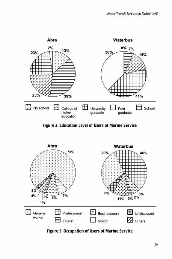
99
Water-Transit Services in Dubai-UAE
Figure 2. Education Level of Users of Marine Service
Figure 3. Occupation of Users of Marine Service

Journal of Public Transportation, Vol. 13, No. 2, 2010
100
Figure 4. Income Level (AED per Month) of Users of Marine Service
These figures indicate that highly-qualified and relatively high-income groups use Waterbus services and low-income groups generally use Abra services. Such pat-terns could be attributed to several reasons. First, there is a difference in the fare of the two marine transport systems, with the Waterbus fare four times higher than that of Abra. Second, there are differences in the surrounding land uses of the sta-tions. For example, S1, S2, and S3 are surrounded by traditional old market areas of Dubai, while S5 and S6 are surrounded mainly by offices and S4 is surrounded by a mixed use of marketplaces and offices. Third, the network itself does not allow a choice between the two modes for any destination (except for S3 and S4 from 12:00 midnight to 6:00 a.m.).
Performance of the existing system. The overall mobility rate (denoting the aver-age number of trips per user per day) for the marine transport system (combina-tion of Abra and Waterbus only) was 0.88, while for the Abra system it was 0.89, indicating more or less the same mobility characteristics for both mode users.

101
Water-Transit Services in Dubai-UAE
Figure 5. Frequency of Use of Marine Service
The main purpose for use of the marine transport service was work (Figure 6). About 61 percent of the marine transport users made their trips for work purposes only. On weekdays, it was 80 percent for Abra and 80 percent for Waterbus. On weekends, 22.4 percent was for Abra and 25 percent was for Waterbus. The next higher portion of trip purposes is leisure and shopping; on weekends, more than 70 percent Abra trips and 66 percent of Waterbus trips were made for these purposes. In conclusion, both modes are similar in accommodating the same trip purposes.
Figure 6. Purpose of Use of Marine Service
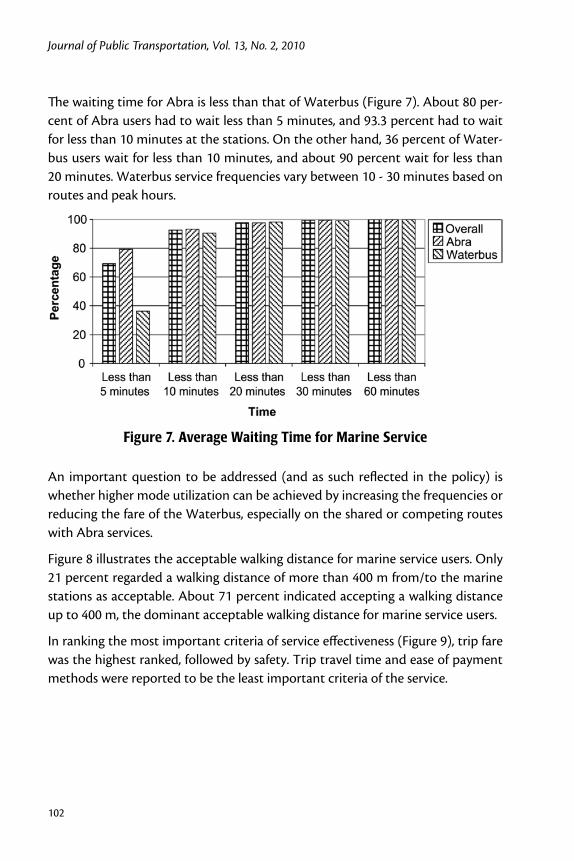
Journal of Public Transportation, Vol. 13, No. 2, 2010
102
The waiting time for Abra is less than that of Waterbus (Figure 7). About 80 per-cent of Abra users had to wait less than 5 minutes, and 93.3 percent had to wait for less than 10 minutes at the stations. On the other hand, 36 percent of Water-bus users wait for less than 10 minutes, and about 90 percent wait for less than 20 minutes. Waterbus service frequencies vary between 10 - 30 minutes based on routes and peak hours.
Figure 7. Average Waiting Time for Marine Service
An important question to be addressed (and as such reflected in the policy) is whether higher mode utilization can be achieved by increasing the frequencies or reducing the fare of the Waterbus, especially on the shared or competing routes with Abra services.
Figure 8 illustrates the acceptable walking distance for marine service users. Only 21 percent regarded a walking distance of more than 400 m from/to the marine stations as acceptable. About 71 percent indicated accepting a walking distance up to 400 m, the dominant acceptable walking distance for marine service users.
In ranking the most important criteria of service effectiveness (Figure 9), trip fare was the highest ranked, followed by safety. Trip travel time and ease of payment methods were reported to be the least important criteria of the service.

103
Water-Transit Services in Dubai-UAE
Figure 8. Acceptable Walking Distance to Marine Station
Figure 9. Most and Least Important Criteria in Ranking Service Effectiveness

Journal of Public Transportation, Vol. 13, No. 2, 2010
104
The willingness to pay a higher fare for service is reported in Figure 10. Nearly 43 percent, 25 percent, and 20 percent of the marine users indicated a willingness to pay a fare increase of 50 percent, 75 percent, or 100 percent, respectively. The reported willingness levels are a bit higher for Abra service users. As for Waterbus users, 33 percent, 15 percent, and 9 percent indicated a willingness to pay for a fare increase of 50 percent, 75 percent, and 100 percent, respectively. Apparently, the willingness levels of Waterbus users to pay a fare increase are less than those of Abra users. This can be explained by the relatively high fare of Waterbus com-pared to Abra.
Figure 10. Willingness to Pay Increased Fares
Figure 11 illustrates user satisfaction levels for the marine services. The user survey shows similar satisfaction levels for both Abra and Waterbus service. A total of 84 percent of marine service users were satisfied, 15 percent were partially satisfied, and only 1 percent were not satisfied with the service.

105
Water-Transit Services in Dubai-UAE
Figure 11. Satisfaction Level with the Marine Service
Existing Intermodal ConnectivityWith regard to the use of other public transportation modes, Abra users indicated the use of bus and taxi, while Waterbus users indicated the use of private car and taxi (Figure 12). The cross-use percentage of Abra and Waterbus is quite minimal and insignificant; very few Waterbus users use Abra, and the use of Waterbus by Abra users is quite rare. One possible reason for this low cross-use-percentage is the rare existence (only for R2 and B4 routes) of a choice between Abra and Water-bus on different routes.
Figure 12. Mode of Transportation Regularly Used by Marine Transport Users
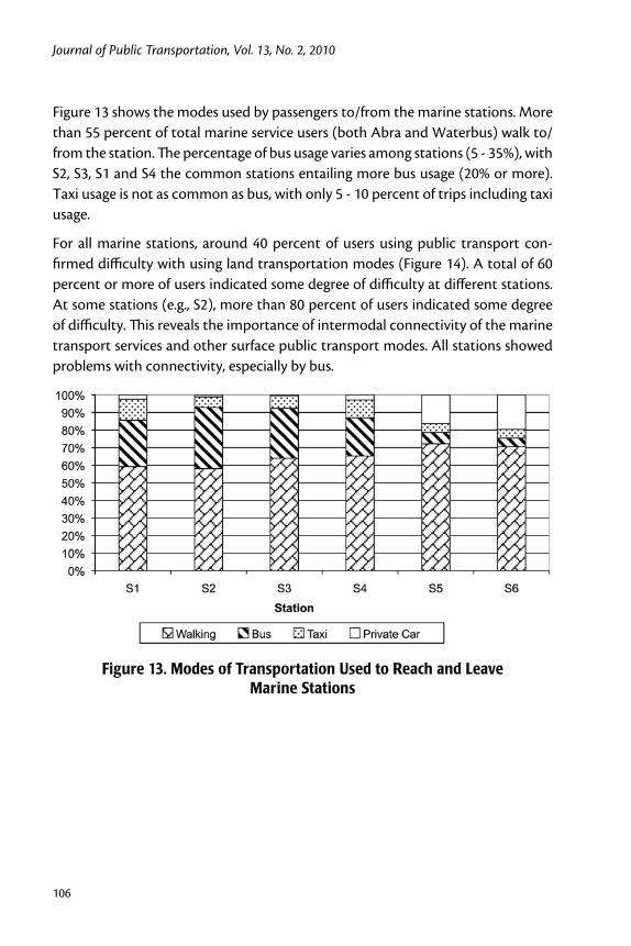
Journal of Public Transportation, Vol. 13, No. 2, 2010
106
Figure 13 shows the modes used by passengers to/from the marine stations. More than 55 percent of total marine service users (both Abra and Waterbus) walk to/fromthestation.Thepercentageofbususagevariesamongstations(5-35%),withS2,S3,S1andS4thecommonstationsentailingmorebususage(20%ormore).Taxi usage is not as common as bus, with only 5 - 10 percent of trips including taxi usage.
For all marine stations, around 40 percent of users using public transport con-firmed difficulty with using land transportation modes (Figure 14). A total of 60 percent or more of users indicated some degree of difficulty at different stations. At some stations (e.g., S2), more than 80 percent of users indicated some degree of difficulty. This reveals the importance of intermodal connectivity of the marine transport services and other surface public transport modes. All stations showed problems with connectivity, especially by bus.
Figure 13. Modes of Transportation Used to Reach and Leave Marine Stations

107
Water-Transit Services in Dubai-UAE
Figure 14. Availability of Public Transport (Bus and Taxi) To/From Marine Stations
Operator SurveyMost Abra operators had good experience with this mode. About 96 percent of Abra operators had more than one year of operating experience in the UAE, and 89.3 percent had the same experience with the current vessel (Figure 15). Water-bus is a relatively new mode (started in 2007). Only 41.6 percent of Waterbus operators had more than one year of experience in the UAE, and only 14.3 percent had more than one year of experience with the current vessel.
Mostoperators (85% forAbraand100% forWaterbus) thought the serviceofthe vessel was good or very good (Figure 16). Most Waterbus operators felt that the Waterbus is safe. However, only 68 percent of Abra operators indicated good safety levels, and 14 percent indicated acceptable levels. In general, the Abra safety level was perceived to be a bit less than that of Waterbus.

Journal of Public Transportation, Vol. 13, No. 2, 2010
108
Figure 15. Experience of Marine Transport Operators in the UAE

109
Water-Transit Services in Dubai-UAE
Figure 16. Level of Service and Safety of Marine Vessels Indicated by Operators

Journal of Public Transportation, Vol. 13, No. 2, 2010
110
With regard to what measures to implement to make the marine service more attractive tousers (Figure17), addingnewer stations (39%), increasing the fre-quencyofoperation(19%),andincreasingthecomfortlevel(19%)wereindicated.On the other hand, operators suggested more frequent updates to roster and operatorschedules(47%)anddecreasingtheservicespantime(29%).
Figure 17. Measures to Increase Attractiveness of Service (Users and Operators)
111
Water-Transit Services in Dubai-UAE
Additional Discussion of Survey FindingsFrom the user survey, trip fare was found to be the most important criteria for service effectiveness (see Figure 9). Respondents also suggested a reduction in fare for Waterbus service. Some Abra users showed interest in shifting to Waterbus if the price were reduced by 50 percent. Ahmed et al. (2009) investigated the price elasticity of Waterbus in Dubai and found it to be elastic. This means that a reduc-tion in the trip fare would increase revenue earnings.
Currently, there is no database of the marine transport system except collected records of monthly passenger counts. Establishing a database for the marine trans-port system could assist in better planning, operational, and management aspects of the system. The database platform could be such that it can support GIS analy-sis. For example, the authority can use GIS technology to manage routes, define locations to establish new stations, define influence/catchments areas of each station, prioritize routes based on demand, etc. Furthermore, interaction with Google maps can help users choose the routes and plan their journey in advance.
During the study, the authors observed a deficiency of quality waiting areas and toilet and wash facilities in the stations. This point also was raised by some respon-dents (users and operators). Users also indicate some difficulties with intermodal connectivity to and from the marine stations, especially by bus. Improving these conditions could increase the ridership of current users and may encourage non-users to start using the marine services.
As previously indicated, one of the limitations of this study was the exclusion of non-users or prospective users in the survey process. A further study should be conducted to identify prospective users and find means to increase the ridership of the marine services. Nonetheless, from the results collected in this study and the above discussion, the following improvements are suggested:
Consideration should be given to reducing the service fare for Waterbus. •This service may earn more revenue by reducing the fare.
The level of comfort for users should be enhanced by providing better •facilities at stations, including better shading and air-conditioned waiting locations, toilets, and washrooms.
A database for the marine transport system should be developed that could •be used for planning, operational, and management purposes. The database platform should support GIS analysis.

Journal of Public Transportation, Vol. 13, No. 2, 2010
112
Initiatives should be undertaken by MA-RTA to develop a good intermodal •connectivity to and from the marine stations, including public bus stops near stations, more bus routes with good frequency, and more parking spaces for private cars.
ConclusionThe majority of assessment tools for the operation practice of MA-RTA services indicated quite acceptable levels of services. Nonetheless, some areas of deficien-cies exist. Success of MA-RTA services requires adequate planning and maximiza-tion of linkage and connectivity among marine services and land public transport facilities. While MA-RTA services might not be profitable, they are a critical sector in complementing all other RTA services. In this perspective, business opportuni-ties of MA-RTA services should be looked at as those that could help reduce the “marginal” cost on all existing transport services (i.e., marine and land services). A profitable project is the one whose capital cost plus long-run operational costs are compromised by the profit of the service itself as well as the overall reductions in (direct and indirect) costs among all other modes of transportation.
Acknowledgment
This research was funded by the MA-RTA project number MR014. The authors would like to acknowledge the efforts of Farida Yaqoob, Hussain Al Saffar, and Sarah Mohammad of MA-RTA for their valuable contributions and feedback throughout the study.
References
Ahern, A. A., and N. Tapley. 2008. The use of stated preference techniques to model modal choices on interurban trips in Ireland. Transportation Research Part A 42: 15–27.
Ahmed F., Y. E., Hawas, M. Hassan, M. Maraqa, and M. B. Khan. 2009. A framework for the assessment and policy development of the water-transit services in Dubai, UAE, submitted to Journal of Public Transportation.
Ceder, A. 2006. Planning and evaluation of passenger ferry service in Hong Kong, Transportation, 33(2), 133-152.

113
Water-Transit Services in Dubai-UAE
Dunlop G. 2002. The European ferry industry: Challenges and changes. Interna-tional Journal of Transport Management 1(2): 115-116.
Espino, R., J. De D. Ortu´zar, and C. Roma´n. 2007. Understanding suburban travel demand: Flexible modelling with revealed and stated choice data. Transporta-tion Research Part A 41: 899–912.
Lai, M. F., and H. K. Lo. 2004. Ferry service network design: Optimal fleet size, rout-ing and scheduling, Transportation Research Part A 38(4): 305-328.
MBTA. 2006. Service Delivery Policy. Massachusetts Bay Transportation Authority.
Melissa, M. L., and G. D. Michael. 2007. Ferry service market analysis: National Parks of New York Harbor. Transportation Research Record 1793: 99-105.
Miller, I. R., J. W. Freund, and R. Johnson. 1990. Probability and Statistics for Engi-neers, 4th edition. Prentice Hall Inc., New Jersey.
Odeck, J., and S. Brathen. 2009. The efficiency of Norwegian ferries in providing public transport services. International Journal of Transport Economics 36(1): 121-139.
Outwater, M. L., S. Castleberry, Y. Shiftan, M. Ben-Akiva, Y. S. Zhou, and A. Kup-pam. 2003. Attitudinal market segmentation approach to mode choice and ridership forecasting: Structural equation modeling. Transportation Research Record 1854: 32-42.
Pickrell, S., and L. Neumann. 2000. Use of performance measures in transportation decision making. In Performance Measures to Improve Transportation Systems and Agency Operations, Transportation Research Board, Irvine, California.
Polak, J., and P. Jones. 1995. Using stated-preference methods to examine trav-eler preferences and responses. In Understanding Travel Behaviour in an Era of Change, eds. P.R. Stopher and M.E.H. Lee-Gosselin, Pergamon-Elsevier, Oxford.
Russell, S. E., and V. A. Eugene. 1999. Intermodal ferry terminal master plans for Washington State Ferries: Planning for the future. Transportation Research Record 1677: 105-116.
Wilson, B. 2005. Waterborne transit: On the move in Southeast Florida. Transpor-tation Planning 30(1): 6-7.

Journal of Public Transportation, Vol. 13, No. 2, 2010
114
About the Authors
Mohammad Nurul Hassan ([email protected]) is a research assistant at the Roadway, Transportation and Traffic Safety Research Center (RTTSRC) at UAE University. He has an M.Sc. degree in Urban and Regional Planning from Bangladesh University of Engineering and Technology. His research focuses on land use and transport planning and policy.
Yaser E. Hawas ([email protected]) currently serves as a professor in the Department of Civil and Environmental Engineering at UAE University, where he also serves as Director of the RTTSRC. He obtained his Ph.D. from the Civil Engineering Department at the University of Texas at Austin in 1996 and joined UAE University in 1998. He has published more than 40 international journal and conference papers and has carried out several professional studies and consultancy works for local and international agencies including the Texas Department of Transportation (US), the Federal Highway Administration, Holden Vehicle Manufacturers (Australia), the United Nations (ESCWA), and many others in the UAE.
Munjed Maraqa ([email protected]) is an associate professor in the Depart-ment of Civil and Environmental Engineering at the UAE University. He has a Ph. D. degree in Environmental Engineering from Michigan State University. His research focuses on mass transfer in porous media. He also is associated with the RTTSRC at UAE University and maintains a research interest in environmental issues associ-ated with transportation.
Faisal Ahmed ([email protected]) is a research assistant at the RTTSRC at UAE University. He obtained his M. Sc. degree in Civil Engineering from Chalmers University of Technology (CTH) in Sweden. His research focuses on traffic engineer-ing, transport planning, and ITS.
Md Bayzid Khan ([email protected]) is an M. Sc. student and a research assistant at the RTTSRC at UAE University. He has a B.Sc. degree in Urban and Regional Planning from Bangladesh University of Engineering and Technology and a keen interest in GIS applications in transport planning and accident research.

115
Investment Decision Making for Alternative Fuel Public Transport Buses
Investment Decision Making for Alternative Fuel Public Transport
Buses: The Case of Brisbane Transport
Anish Patil and Paulien Herder Delft University of Technology
Kerry Brown
Southern Cross University
Abstract
Cleaner and less polluting public transport buses based on alternative fuels are of paramount importance if cities are to attain their ambitious emissions reduction tar-gets. Public transport buses are high usage vehicles that operate in heavily congested areas where air quality improvements and reductions in public exposure to harmful air contaminants are critical. As such, they are good candidates for achieving both near-term and long-term emission reductions. Decision making for the investment in alternative fuel buses is dependent on future technological development and emissions standards, and it is difficult, given the uncertainty in regards to both these factors. The objective of this paper is to develop an analytical framework that will give us more insight into the trends in emissions standards as well as technology development, and eventually translate these insights into a sound investment deci-sion making strategy. This paper concludes that, due to presence of uncertainties, the decision maker (public transport fleet manager) can take only incremental steps that will allow him or her to safeguard investments. Furthermore, if policy makers

Journal of Public Transportation, Vol. 13, No. 2, 2010
116
are serious about accelerating the diffusion of alternative fuels, they should aim at creating stable policy environment.
IntroductionCities around the world have set ambitious emissions reduction targets. The pri-mary environmental objective of any city is to reduce human exposure to harm-ful pollutants while at the same time not hindering the movement of people. This objective can be achieved in two ways—reduce the number of vehicles and reduce the pollution from each vehicle. The number of vehicles can be reduced by improving public transport and simultaneously encouraging residents to use public transport instead of driving their personal automobiles. Pollution from each vehicle can be reduced by promoting the use of alternative fuel vehicles that have lower emissions. Given the potential of alternative fuels as a clean and safe energy resource, they can be expected to play a larger role powering the transport sector in the future. Cleaner and less polluting public transport buses based on alternative fuels are of paramount importance if cities are to attain their ambitious emissions reduction targets, as public transport buses are high usage vehicles that operate in heavily congested areas where air quality improvements and reductions in public exposure to harmful air contaminants are critical. As such, they are good candidates for achieving both near-term and long-term emissions reductions, as many buses are centrally kept and fueled, making the introduction of new tech-nologies and alternative fuels more efficient (Kojima 2001).
This paper establishes the importance of emissions standards and technological development during the decision making process of procurement of new public transport buses. A bus has a life expectancy of about 20 years. If the emissions standards change during the lifespan of a bus and if it can no longer satisfy the requirements, the bus has to be phased out or upgraded to comply with the emissions standards requirements—which cost time and money, thus leading to financial and service losses. The objective of a decision maker while investing is to optimize the returns of his/her investments—low costs for high returns. Given the long life span of the buses, a decision maker is faced with a number of uncertainties while making the investment decision. These uncertainties are related to the pro-gression of the technology development and emissions standards for diesel buses, i.e., the pace at which they will become more stringent and the development of technology over time. Numerous strategies can be employed to face this uncer-tainty (Walker et al. 2001; Kim and Sanders 2002), including delay of decision, do

117
Investment Decision Making for Alternative Fuel Public Transport Buses
further research, implement a flexible solution, implement a robust solution, take incremental steps by implementing a solution that builds on the existing compe-tencies, etc.
This paper focuses on Brisbane Transport as a case study. The aim is to develop an analytical framework that will allow insight into both the trends in emissions standards and technology development, eventually translating these insights into sound investment decision making. First, the paper discusses the types of uncer-tainties and their impact on the investment decision making strategy. Second, the Brisbane Transport case study is introduced. Third, different alternative fuel tech-nologies for public transport buses and their characteristics are discussed. Fourth, the paper focuses on the trends in emissions standards for public transport buses and how they affect the public transport fleet manager in their procurement strat-egy. Finally, recommendations are given with respect to the implications for future emissions standards trends and the choice of alternative fuel buses for the fleet by applying this to Brisbane case study.
Impact of uncertainties on investment decision making The transport sector is capital intensive, and investments are characterized by longevity of technological components and irreversibility due to the large up-front sunk costs. In addition, there are different sources of uncertainty that have an impact on investment decisions, such as the uncertainty about the pace and direc-tion of technological developments and uncertainty about future policy and regu-lations (Meijer et al. 2007). Technological uncertainty can relate to the technology itself, to the relation between the technology and the technological system, or to the availability of alternative technological solutions (both technologies that are already available as well as technologies that might become available in the future) (Meijer 2008). Furthermore, uncertainty can emerge about current policy (e.g., uncertainty about the interpretation or effect of policy, or uncertainty due to a lack of regulation) or about future changes in policy. Uncertainty about gov-ernmental behavior (policies) is also an important cause for political uncertainty (Meijer 2008) and, as such, can have a detrimental impact on the diffusion of new alternative fuel technologies. The decision of any actor to invest in alternative fuel technology buses is highly influenced by governmental policies, which determine the “rules of the game”; if the policies are uncertain, then it sends wrong signals to the decision makers and shows that the government is not serious about transi-tion towards sustainability. There are many rules and regulations affecting the

Journal of Public Transportation, Vol. 13, No. 2, 2010
118
decision making process, but the most relevant of those that directly affect the investment decision making is emissions standards (Welsh 2007).
Decision making for procurement of new buses is heavily based on the emissions standards, as every new bus should comply with the corresponding emissions standards (AATA 2002; Hao et al. 2006). In case a new bus satisfies the “current most stringent emissions standards,” then that bus often is selected (Welsh 2007). What makes the job of the decision maker difficult is the uncertainty regarding future emissions standards, coupled with the fact that many competing alterna-tive fuel technologies are still unproven and their long term impact is yet unknown (WSU 2004). A bus has a life expectancy of about 20 years (Welsh 2007); during its lifespan, if the emissions standards change and the bus can no longer satisfy the requirements, then it has to be phased out or upgraded to comply with the emis-sions requirements. The objective of a decision maker while investing is to optimize the returns of investments – low costs and lower emissions. The new buses should have to be reliable, efficient, and environmentally-friendly and, at the same time, be cost effective in terms of purchasing price, operation and maintenance in order to optimize the taxpayer’s resources. Any decision today could have repercussions for the next 25 years or so as the life cycle of a regular bus constitutes 20 years in addition to a lag time of about 4 to 5 years for the process of order and delivery.
In this paper, although we consider that the decision maker is a public transport fleet manager, at the same time we are aware that these decisions are influenced by many political players, a characteristic of every public sector governance envi-ronment. Decisions to invest in alternative fuel technology are politically sensitive and influenced by strategic and political reasons (Wüstenhagen et al. 2007). The analytical framework we propose in this paper has the ability to take into account factors such as political sensitivity and other external inputs that affects the deci-sion making process; however, to keep this discussion and our recommendations crisp, we focus only on emissions standards and technological developments. The aim of the framework is to show that investment decision making is impacted by both social and technical components. The public transport sector is a socio-technical system (STS), as it combines social and technical components that inter-act and function together (Ottens et al. 2006). Social components include actors, rules, regulations, etc; technical components include machinery, buses, etc. An analysis of such systems cannot focus only on technological components; equal relevance should be given to social components (Weijnen et al. 2008; Bauer and

119
Investment Decision Making for Alternative Fuel Public Transport Buses
Herder 2009). It is the interaction between these components that determine the direction of system development.
Analytical FrameworkWe use the socio-technical systems perspective to analyze the problem of invest-ment decision making; such perspective allows the collective analysis of the social and technical components. Our analytical framework as described below is devel-oped to capture the interactions within the transport sector. The framework ana-lyzes technology, actors and rules—technology refers to the physical network such as machinery, buses, engines, etc; actors refer to the presence of the multi-actor network; and rules refer to regulations and standards. Rules can be classified as for-mal and informal rules. Formal rules include operational standards (interoperabil-ity, process), technical standards (engineering practices), organizational standards (management styles), environmental standards (such as emission limit values), etc. Informal rules include norms, cultures, traditions, etc. Rules are not mere con-structs but part of the system; standards co-evolve during the development of the socio-technical systems, and they change or are changed as system functionalities are modified. As shown in the Figure 1, the analytical framework accentuates the interactions within the various components of an STS. For example, actors create rules and, at the same time, the behavior of the actors is more or less governed by rules; technology development is constrained by the prevailing system of rules, and rules are shaped by the current technology status; and, finally, actors create and manage technology and, at the same time, technology influences actor behavior.
All the three components of a socio-technical system are interdependent; actors, rules and technology interact with each other for the proper functioning of an STS. This implies that the actors’ decision making is influenced by both the rules and the technology. As discussed earlier, the aim of this paper is to provide recom-mendations to the decision maker while investing in alternative fuel technology buses. To gather insight into this decision making process, we apply our analytical framework to a case study, Brisbane Transport.

Journal of Public Transportation, Vol. 13, No. 2, 2010
120
Figure 1. Interactions within a Socio-Technical System
Brisbane Transport case studyThe Brisbane City Council predicts huge population growth in Brisbane, especially in the suburbs. With population growth comes more traffic, more vehicles, more emissions; hence, the Brisbane City Council in its Living in Brisbane 2026—Vision for Brisbane and Climate Change and Energy Taskforce—A Call for Action docu-ments identified safe, reliable and clean public transport as a means to keep Bris-bane’s air clean and reduce green house gas emissions to counteract the impacts of climate change (Brisbane-Council 2006).
Brisbane Transport is a business unit of the Brisbane City Council, operating subur-ban and urban bus services in the Brisbane metro area. The current Brisbane trans-port fleet is 1053 buses (as of Jan 2010) (www.brisbanetransport.info/fleetlist.php). The fleet has a balance of CNG (compressed natural gas) and diesel buses (ratio 60:40). Since the year 2000, only CNG buses have joined the fleet. In line with the

121
Investment Decision Making for Alternative Fuel Public Transport Buses
above mentioned 2026 Vision documents, Brisbane Transport has formulated two strategies to achieve the 2026 vision for Brisbane: increase bus patronage from the existing 67 million to 110 million and add cleaner (i.e., lower emissions) buses to the fleet. Brisbane Transport has estimated that a fleet of 1,785 buses will allow it to reach its 2026 patronage targets (Brisbane-Council 2007). About 85 new buses should join the fleet every year in order to have 1,785 buses in 2026. This number accounts for the older buses that will be withdrawn after 20 years of service life. Hence, about 1,500 new buses will be joining the fleet from 2010 until 2026.
Overview of alternative fuel technologies for busesThere are numerous alternative fuel technologies for public transport buses avail-able in the market; most notable are clean diesel buses, compressed natural gas (CNG) buses, hythane buses, hybrid buses and fuel cell buses powered by pure hydrogen (AATA 2002; WSU 2004). In this section, we discuss, compare and con-trast these technologies.
Clean Diesel BusesThere have been tremendous innovations in diesel engine technology over the past few years—for example, advanced engine electronic combustion control, fuel injection systems and turbochargers to optimize performance and lower the emissions (Gifford 2003). Advanced low-sulphur fuels are available in the market. These cleaner diesel fuels produce lower emissions and enable advanced emissions treatment systems (catalysts and filters). Lower amount of sulphur in diesel fuel enables catalytic converters to be used, which, in turn, lower carbon monoxide (CO), nitrogen oxide (NOx) and hydrocarbon (HC) emissions. Emis-sions treatment such as particulate filters and oxidation catalysts reduce emissions of ozone-forming compounds (NOx and HC) and trap and eliminate particulate matter (PM) (Gifford 2003; Kassel and Bailey 2004). Currently, diesel emissions are reduced by turbo-charging, after-cooling, high pressure fuel injection, retard-ing injection timing and optimizing combustion chamber design. Turbochargers reduce both NOx and PM emissions by approximately 33 percent when compared to naturally-aspirated engines. Combustion chamber improvements and air-fuel injection advancements are ongoing in the industry and result in improved fuel economy and emission reductions (WSU 2004). As diesel engine improvements have already reached their limit, NOx and PM emission control requires after-treatment devices to satisfy new, stringent emissions standards.

Journal of Public Transportation, Vol. 13, No. 2, 2010
122
CNG BusesNatural gas (NG) has been proposed as a much cleaner alternative to conventional diesel. Consisting primarily of methane and other light hydrocarbons, natural gas does not contain hydrocarbons that form harmful emissions. In fact, the principal source of particulate emissions from natural gas vehicles is the combustion of lubricant. Replacing heavy-duty diesel vehicles with CNG equivalents is one option for reducing vehicular particulate emissions dramatically (DOE 2002; Tzeng et al. 2005). Many cities have started investing in CNG buses. For example, cities such as Mumbai and Delhi have completely shifted their fleet from diesel buses to CNG buses (Yedla and Shrestha 2003); for cities in developing countries such as India, CNG buses offers low emissions and cost-effective public transport.
Hythane BusesCNG buses are looked upon as a potential alternative to diesel buses – they are less polluting and the fuel is widely available. However, in an effort to reduce their pollutants further, CNG buses can be converted to run on hythane (Bauer and For-est 2001). Mixtures of hydrogen and natural gas are considered viable alternative fuels to lower overall pollutant emissions but suffer from problems associated with on-board storage of hydrogen, resulting in limited vehicle range (Nagalingam et al. 1983; Karim et al. 1996). Hythane, a patented product, is a mixture of 20 percent by volume of H2 and 80 percent methane (Hythane 2007). The laboratory for Trans-port Technology at University of Gent in Belgium has done considerable research on the suitability of hythane for public transport buses. In its experiment, a city bus with an adapted MAN CNG engine was tested on a chassis dynamometer at four speeds (30, 50, 70 and 80 km/h) with natural gas and hythane (HydroThane 2004). The same load conditions at the same speed were realized for the two fuels so that exhaust emissions concentrations can be compared. The averages over the four speeds of the exhaust gas concentrations with hythane as a fuel compared to natural gas are 66 percent reduction of unburned hydrocarbons (HC), 32 percent reduction of nitrogen oxides (NOx), 17 percent reduction of carbon monoxide (CO), and 13 percent reduction of carbon dioxide (CO2). Experiments at the Uni-versity of Lund and City of Malmo gave similar results for hythane (Ridell 2005). There are many cities in the world that are experimenting with hythane, such as the Beijing Hythane Bus Project, whose demonstration phase will be to adapt 30 natural gas engines for hythane operation (Ortenzi et al. 2007).

123
Investment Decision Making for Alternative Fuel Public Transport Buses
Hybrid BusesAn emerging alternative to conventional diesel engines is electric hybrid bus tech-nology. Hybrid buses typically use an electric drive coupled in series or operating in parallel with a combustion engine and traction battery. Hybrid technology allows the use of a smaller internal combustion engine that is designed to operate near its optimum efficiency, thereby minimizing engine emissions and maximizing fuel economy. Typically, a hybrid system also employs regenerative braking, which transforms kinetic energy into electric energy, again improving fuel economy. To a fleet operator, hybrid technology is attractive because it does not require the development of new refueling infrastructure or modifications to existing mainte-nance areas (WSU 2004; Tzeng et al. 2005).
Fuel Cell BusesFuel cell buses run on hydrogen, which can be stored on board in high pressure cyl-inders or could be produced on board through natural gas or methanol. There are many cities in the world currently experimenting with fuel cell buses; for example, the Clean Urban Transport for Europe (CUTE) is a European Union project that saw the development and testing of 27 hydrogen fuel cell buses, three in each of nine cities in Europe (CUTE). This technology is still in its experimental phase; it will be few years before it is commercialized. The main advantage of using fuel cell buses is zero tailpipe emissions, but there are many drawbacks. Obtaining hydro-gen fuel is difficult, as hydrogen does not exist in free form in nature. Hydrogen has to be produced from either natural gas or electrolysis that makes it an expensive fuel. Bus prices are currently exorbitant compared to other alternative fuel buses, thus putting this technology out of reach of many public transport authorities (Tzeng et al. 2005).
Table 1 summarizes the comparative assessment of different alternative fuel tech-nologies. The criteria for analysis is maturity of technology, cost of production and operation, safety and performance. As can be seen in the table, hybrid and fuel cell technologies are the cleanest and have the highest potential to reduce emissions. Yet, at this point, they are in the development phase and long-term reliability is yet unknown. This, coupled with the fact that they are exorbitantly expensive, makes them an unattractive choice. CNG technology is quite clean and over the years has proved efficient in reducing emissions when compared to diesel buses., Given their affordability and reliability, many cities around the world are moving to CNG buses. To further reduce emissions from CNG buses, hydrogen could be added to CNG to create hythane buses. This combines the strengths of both CNG
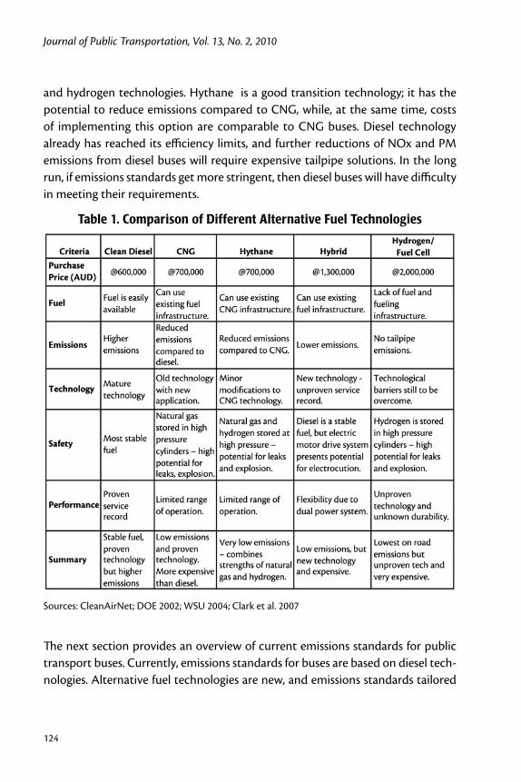
Journal of Public Transportation, Vol. 13, No. 2, 2010
124
and hydrogen technologies. Hythane is a good transition technology; it has the potential to reduce emissions compared to CNG, while, at the same time, costs of implementing this option are comparable to CNG buses. Diesel technology already has reached its efficiency limits, and further reductions of NOx and PM emissions from diesel buses will require expensive tailpipe solutions. In the long run, if emissions standards get more stringent, then diesel buses will have difficulty in meeting their requirements.
Table 1. Comparison of Different Alternative Fuel Technologies
Sources: CleanAirNet; DOE 2002; WSU 2004; Clark et al. 2007
The next section provides an overview of current emissions standards for public transport buses. Currently, emissions standards for buses are based on diesel tech-nologies. Alternative fuel technologies are new, and emissions standards tailored

125
Investment Decision Making for Alternative Fuel Public Transport Buses
for their performance are yet to evolve. For example, at this point, alternative fuel buses such as CNG have to satisfy equivalent diesel bus emissions standards.
Emissions from diesel buses and emissions standardsEmissions from diesel engines are the byproducts of the combustion of the fuel. As per a British Petroleum (BP) fact sheet, for every 1kg of diesel burned, there is about 1.1kg of water (as vapor/steam) and 3.2kg of carbon dioxide produced. Unfortunately, as there is no 100 percent combustion, there is also a small amount of byproduct of incomplete combustion: carbon monoxide, hydrocarbons, and soot or smoke. In addition, the high temperatures that occur in the combustion chamber promote an unwanted reaction between nitrogen and oxygen from the air. This results in various oxides of nitrogen, commonly called NOx (BP 2002). Fig-ure 2 shows the composition of different gases in diesel engine exhaust. Exhaust from the public transport buses typically contains:
Particulate matter (PM) – soot •
Nitrogen oxides (NOx) – lung irritant and smog. •
Carbon monoxide (CO) – poisonous gas•
Hydrocarbons (HC) – smog•
Carbon Dioxide (CO• 2) – Greenhouse gas
Figure 2. Exhaust from diesel buses

Journal of Public Transportation, Vol. 13, No. 2, 2010
126
Particulate matter is the general term for the mixture of solid particles and liquid droplets found in the air. Particulate matter includes dust, dirt, soot, smoke and liquid droplets. It can be emitted into the air from natural and manmade sources, such as windblown dust, motor vehicles, construction sites, factories and fires. NOx emissions produce a wide variety of health and welfare effects. NOx can irritate the lungs and lower resistance to respiratory infection (such as influenza). NOx emissions are an important precursor to acid rain that may affect both ter-restrial and aquatic ecosystems. CO is the product of the incomplete combustion of carbon-containing compounds (Cohen 2005). CO contributes to green house gas effects and global warming. HC comprises unburned hydrocarbons in the fuel; it contributes to smog (blue haze over heavily populated cities). Although CO2 emissions are more than 75 percent of the total emissions, and it is a green house gas (GHG) and has a huge global warming potential, it is still not mandatorily regu-lated by emissions standards. This will be elaborated further in the next section.
Emissions StandardsEmissions standards are minimum compliance requirements that set the upper limits for the amount of pollutants a vehicle can emit into the air. Emissions standards for heavy duty diesel vehicles generally limit the exhaust emissions of four pollutants (DieselNet; Walsh 2000): nitrogen oxides (NOx), particulate mat-ter (PM), hydrocarbons (HC), and carbon monoxide (CO). Carbon dioxide (CO2) emissions correlate to the fuel efficiency of the vehicle and are not limited by emis-sions standards. For example, the current European emissions standards do not set limits for CO2 emissions—CO2 is controlled through voluntary agreements with the automobile manufacturers. Australian public transport buses are subject to European Union (EU) emissions standards. They are a set of requirements outlin-ing the limits for tailpipe exhaust emissions for new vehicles sold in Australia. The emissions standards are defined in a series of EU directives—emissions standards for new heavy-duty diesel engines are commonly referred to as Euro I through Euro V (DieselNet). Euro I standards were introduced in 1992, as shown in Figure 3, over the period 1992-2008; the permissible NOx emission limits have reduced by 75, PM limits have reduced by over 97 percent, HC limits have reduced by 58 percent, and CO limits have reduced by 67 percent. Currently, Australian public transport buses should satisfy Euro IV standards (DOTARS ; DOTARS 2004).

127
Investment Decision Making for Alternative Fuel Public Transport Buses
Figure 3. Changes in Emissions Limits, as a % of 1992 Limits
Results of the current stricter emissions standards could be witnessed within the next 15-20 years. As can be seen in Figure 4, over the next 10 years, NOx, PM, HC and CO are projected to decrease in Australia, but CO2 concentration is forecasted to increase in the future (Walsh 2000; Schulte-Braucks 2006). Improve-ments in diesel technology and fuels have made this possible, and this transition has resulted in heavy-duty diesel engines that are more reliable, durable and less polluting than the diesel engines of the past (Scheinberg 1999). On the other hand, carbon dioxide emissions from road transport are forecasted to increase in the future due to increases in the number of vehicles. Carbon dioxide is not regulated through emissions standards; carbon dioxide emissions are a function of the vehicle’s fuel efficiency, which is regulated with voluntary agreements with vehicle manufacturers.

Journal of Public Transportation, Vol. 13, No. 2, 2010
128
Figure 4. Projected Emissions for Key Pollutants for Australia
DiscussionCNG buses are inherently clean and are capable of reducing emissions, but, consid-ering the 2026 clean air targets, Brisbane Trasnport should invest in hythane buses. Hythane buses will allow Brisbane Transport to considerably lower NOx and GHG emissions at only a marginally higher cost than CNG buses. Existing CNG buses can be easily converted to hythane buses with minor modifications. Natural gas regulators and carburetors are converted with only minor modifications, such as change of spring to accommodate the lighter gas (Nagalingam et al. 1983). Cur-rent hybrid and fuel cell bus technology is still immature and entails high invest-ment costs for these buses. Although hybrid buses have higher fuel efficiency, the technology is undeveloped and has high maintenance and repair costs that do not warrant the investment in such expensive technology. Fuel cell and hydrogen buses are in their infancy and experimental phase—hence, huge investments in this technology should be avoided at this time unless subsidized by the Australian or Queensland government. The decision making process outlined in this research indicates that Brisbane Transport should invest in hythane buses for the future. Given the uncertainties about future policies and technology development, the hythane option entails incremental steps that build upon existing proven CNG technology. Also, hythane buses can use the existing CNG infrastructure with minor modifications. Brisbane Transport would be well positioned to convert its older CNG bus fleet into hythane with the introduction of stricter emissions stan-

129
Investment Decision Making for Alternative Fuel Public Transport Buses
dards, as hythane buses are better poised to deal with the uncertainties in future emissions standards.
ConclusionEmissions standards can create incentives for the transition towards sustainability. Over the years, as emissions standards have become more stringent, bus manufac-turers and fuel producers have developed numerous innovations (advanced engine electronic combustion control, fuel injection systems, and turbochargers to opti-mize performance) to increase thermal efficiency and reduce emissions in order to comply with the standards. Looking at the trends in emissions, it is observed that the aggregate amount of PM, NOx, CO and HC (mandatorily controlled by emissions standards) in the air due to transport has reduced over the years and is forecasted to further reduce, in spite of increases in number of vehicles. The framework developed in this paper gives insight into the interactions between the actors, rules and technology components of the transport sector and highlights the way policies affect technology development and actor decision making. Due to the uncertainties about future policy rules, the decision makers should take incremental steps (build on the existing competencies) to safeguard investments. Hence, we recommend an incremental change by investing in hythane technology buses for Brisbane Transport, as this will safeguard investments for the decision makers in the short term. If the government aims at accelerating the diffusion of alternative fuel technologies, it should create a stable policy framework. Such a policy framework would give an idea to the decision makers about the future progression of rules and regulations. As seen from the case study, voluntary agree-ments to reduce CO2 have so far been unsuccessful; future emissions standards should aim at mandating CO2 emissions.
Although decision making for the procurement of new buses is an important issue for transit authorities to achieve future environmental targets, little research has been done to date to assist the fleet manager in making these procurement decisions. This research aims to bridge this gap in the literature. The decision making process outlined in this research, based on forecasting, trend analysis and technology assessment, is adaptable to other types of infrastructure decisions to enable strategic procurement. We understand that there is a larger scope for improvement in terms of future research; this research was done for the Brisbane Transport and is by no means comprehensive, as it ignores many other sources of uncertainty and limitations faced by a decision maker during procurement. Future
Journal of Public Transportation, Vol. 13, No. 2, 2010
130
research should be more comprehensive and could build on the analytical frame-work discussed in this paper to develop a decision making tool for the benefit of public transport authorities.
Acknowledgement
The author would like to thank CIEAM (Co-operative Research Center for Engi-neering Asset Management), Australia for facilitating this research.
References
AATA. 2002. Alternative fuels, emissions & technology. White paper. Ann Arbor, Ann Arbor Transportation Authority.
Bauer, C. G., and T. W. Forest. 2001. Effect of hydrogen addition on the perfor-mance of methane-fueled vehicles. Part I: Effect on S.I. engine performance. International Journal of Hydrogen Energy 26(1): 55-70.
Bauer, J. M., and P. M. Herder. 2009. Designing Socio-Technical Systems. Handbook of the Philosophy of Science. A. Meijers, Elsevier.
BP. 2002. Diesel engine emissions. www.bp.com.au/fuelnews.
Brisbane-Council. 2006. Our shared vision - Living in Brisbane 2026, Brisbane City Council.
Brisbane-Council. 2007. Transport Plan for Brisbane 2006-2026 (Draft). Brisbane, Brisbane City Council.
Clark, N. N., and F. Zhen et al. 2007. Transit Bus Life Cycle Cost and Year 2007 Emissions Estimation. Washington, D.C., U.S. Department of Transportation Federal Transit Administration.
CleanAirNet. Advanced diesel bus. Clean Air Initiative.
Cohen, J. T. 2005. Diesel vs. compressed natural gas for school buses: A cost-effec-tiveness evaluation of alternative fuels. Energy Policy 33(13): 1709-1722.
CUTE. HyFLEET - Clean urban transport for Europe. www.global-hydrogen-bus-platform.com/About/History/CUTE.
DieselNet. Emission standards. www.dieselnet.com/standards/.

131
Investment Decision Making for Alternative Fuel Public Transport Buses
DOE 2002. Alternative fuels in public transit: A match made on the road. Depart-ment of Energy, USA (Office of Scientific and Technical Information).
DOTARS. Australia design rules - Vehicles and the environment. www.dotars.gov.au/roads/motor/design/adr_online.aspx.
DOTARS. 2004. Regulation impact statement for vehicle emissions and fuel qual-ity standards for the post 2006 period. Department of Transport and Regional Services on behalf of Land Transport Environment Committee.
Gifford, K. 2003. Advances in diesel engine technology. Clean Diesel Conference, Denver, Diesel Technology Forum.
Hao, J., and J. Hu et al. 2006. Controlling vehicular emissions in Beijing during the last decade. Transportation Research Part A: Policy and Practice 40(8): 639-651.
HydroThane. 2004. Clean Technology for Public Transport (CTPT) - Hydrogen as a renewable alternative for diesel and gasoline.
Hythane. 2007. Hythane - Blue Sky, Clean Air. www.hythane.com/.
Karim, G. A., and I. Wierzba et al. 1996. Methane-hydrogen mixtures as fuels. Inter-national Journal of Hydrogen Energy 21(7): 625-631.
Kassel, R., and D. Bailey. 2004. Cleaning up today’s dirty diesels - Retrofitting and replacing heavy duty vehicles in the coming decade. National Resources Defense Council.
Kim, Y. J., and G. L. Sanders. 2002. Strategic actions in information technology investment based on real option theory. Decision Support Systems 33(1): 1-11.
Kojima, M. 2001. Breathing clean - Considering the switch to natural gas buses. World Bank Technical Paper. Washington, D.C., World Bank.
Meijer, I. 2008. Uncertainty and entrepreneurial action. The role of uncertainty in the development of emerging energy technologies. Utrecht, Netherlands, Utrecht University.
Meijer, I. S. M., and M. P. Hekkert et al. 2007. How perceived uncertainties influence transitions: The case of micro-CHP in the Netherlands. Technological Forecast-ing and Social Change 74(4): 519-537.
Journal of Public Transportation, Vol. 13, No. 2, 2010
132
Nagalingam, B., and F. Duebel et al. 1983. Performance study using natural gas, hydrogen-supplemented natural gas and hydrogen in AVL research engine. International Journal of Hydrogen Energy 8(9): 715-720.
Ortenzi, F., and M. Chiesa et al. 2007. Experimental tests of blends of hydrogen and natural gas in light duty vehicles. HYSYDAYS - 2nd World Congress of Young Scientists on Hydrogen Energy Systems, Turin.
Ottens, M., and M. Franssen et al. 2006. Modelling infrastructures as socio-techni-cal systems. International Journal of Critical Infrastructures 2(2/3).
Ridell, B. 2005. Malmo hydrogen and CNG/hydrogen filling station and Hythane bus project. Risoe Energy Conference, Roskilde, Denmark.
Scheinberg, P. 1999. Mass transit - Use of alternative fuels in transit buses. Report to Congressional Committee. Washington, D.C., United States General Accounting Office.
Schulte-Braucks, R. 2006. European vehicle emissions regulations. European Natu-ral Gas Vehicles Association Conference, Brussels.
Tzeng, G.-H., and C.-W. Lin et al. 2005. Multi-criteria analysis of alternative-fuel buses for public transportation. Energy Policy 33(11): 1373-1383.
Walker, W. E., S. A. Rahman et al. (2001). Adaptive policies, policy analysis, and policy-making. European Journal of Operational Research 128(2): 282-289.
Walsh, M. P. (2000). Vehicle Emission Trends. Paris, European Conference of Min-isters of Transport.
Weijnen, M. P. C., and P. M. Herder et al. 2008. Designing complex systems: A con-tradiction in terms. In Eekhout, M., R. Visser and T. Tomiyama, Delft Science in Design², A Congress on Interdisciplinary Design 3: 235-254.
Welsh, M. 2007. Importance of emission standards during the procurement of new buses. Brisbane.
WSU. 2004. New engine technologies: Diesel emissions reports. Olympia, Washing-ton, Washington State University - Energy Program.
Wüstenhagen, R., and M. Wolsink et al. 2007. Social acceptance of renewable energy innovation: An introduction to the concept. Energy Policy 35(5): 2683-2691.
133
Investment Decision Making for Alternative Fuel Public Transport Buses
Yedla, S. and R. M. Shrestha. 2003. Multi-criteria approach for the selection of alternative options for environmentally sustainable transport system in Delhi. Transportation Research Part A: Policy and Practice 37(8): 717-729.
About the Authors
Anish Patil ([email protected]) is a researcher at the Faculty of Technology, Policy Management at the Delft University of Technology in The Netherlands. His scientific interests lie in the areas of sustainable infrastructure development and environmentally-conscious industrial planning. His Ph.D. research focuses on model-ing complex, multi-actor energy systems and studying the effects of various policy implications during transition to a more sustainable energy system.
Paulien Herder ([email protected]) is a Professor of Engineering Systems Design in Energy and Industry in the Energy & Industry group at the Delft Univer-sity of Technology and Scientific Director at the Next Generation Infrastructures. She obtained her M.Sc. degree in Chemical Engineering at the Delft University of Technology in 1994. Her Ph.D. research was aimed at the design and design process of chemical plants.
Kerry Brown ([email protected]) is the Mulpha Chair in Tourism Asset Management and Professor in the School of Tourism and Hospitality Management at Southern Cross University in Australia. Her previous role was Professor in the School of Management at Queensland University of Technology and Program Leader for the Cooperative Research Centre for Integrated Engineering Asset Management (CIEAM) Strategic Human Dimensions Program. She is the interim Program Leader for the Organizational Performance and Human Capability Program for CIEAM2.