journal of public transportation - university of south florida
TRANSCRIPT

Factors Influencing Young Peoples’ Perceptions of Personal Safety on Public Transport
An Analysis of Special Needs Student Busing
�e Impact of Hiawatha Light Rail on Commercial and Industrial Property Values in Minneapolis
State and Federal BRT Project Development Procedures: Managing Differences and Project Implementation Delays
Impacts of the Cedar Avenue Driver Assist System on Bus Shoulder Operations
Definition and Properties of Alternative Bus Service Reliability Measures at the Stop Level
Maintaining Key Services While Retaining Core Values: NYC Transit’s Environmental Justice Strategies
A Bus Rapid Transit Line Case Study: Istanbul’s Metrobüs System
Volume 16, No. 1, 2013
Vo
lum
e 16, No
. 1
Jo
urn
al of P
ub
lic Transp
ortatio
n
2013
N C T R
Graham Currie Alexa DelboscSarah Mahmoud
Behrooz Kamali Scott J. MasonEdward A. Pohl
Kate KoXinyu (Jason) Cao
Mark A. Miller
Brian Pessaro
Meead Saberi Ali Zockaie K.Wei Feng Ahmed El-Geneidy
Ted Wang Alex LuAlla Reddy
M. Anıl Yazıcı Herbert S. LevinsonMustafa Ilıcalı Nilgün CamkeseCamille Kamga

Gary L. Brosch, EditorLisa Ravenscroft, Assistant to the Editor
EDITORIAL BOARD
Robert B. Cervero, Ph.D. University of California, Berkeley
Chester E. ColbyE & J Consulting
Gordon Fielding, Ph.D.University of California, Irvine
Jose A. Gómez-Ibáñez, Ph.D. Harvard University
Naomi W. Ledé, Ph.D.Texas Transportation Institute
SUBSCRIPTIONS
Complimentary subscriptions can be obtained by contacting:
Lisa Ravenscroft, Assistant to the EditorCenter for Urban Transportation Research (CUTR)University of South FloridaFax: (813) 974-5168Email: [email protected]: www.nctr.usf.edu/jpt/journal.htm
SUBMISSION OF MANUSCRIPTS
The Journal of Public Transportation is a quarterly, international journal containing original research and case studies associated with various forms of public transportation and re-lated transportation and policy issues. Topics are approached from a variety of academic disciplines, including economics, engineering, planning, and others, and include policy, methodological, technological, and financial aspects. Emphasis is placed on the identifica-tion of innovative solutions to transportation problems.
All articles should be approximately 4,000 words in length (18-20 double-spaced pages). Manuscripts not submitted according to the journal’s style will be returned. Submission of the manuscript implies commitment to publish in the journal. Papers previously published or under review by other journals are unacceptable. All articles are subject to peer review. Factors considered in review include validity and significance of information, substantive contribu-tion to the field of public transportation, and clarity and quality of presentation. Copyright is retained by the publisher, and, upon acceptance, contributions will be subject to editorial amendment. Authors will be provided with proofs for approval prior to publication.
All manuscripts must be submitted electronically in MSWord format, containing only text and tables —no linked images. If not created in Word, each table must be submitted separately in Excel format and all charts and graphs must be in Excel format. Each chart and table must have a title and each figure must have a caption. Illustrations and photographs must be submitted separately in an image file format (i.e., TIF, JPG, AI or EPS), having a minimum 300 dpi and measuring at least 4.5” x 7” in size, regardless of orientation. However, charts and graphs may be submitted for use as spreads, covering two facing pages of an article. Please include all sources and written permissions for supporting materials.
All manuscripts should include sections in the following order, as specified:Cover Page - title (12 words or less) and complete contact information for all authorsFirst Page of manuscript - title and abstract (up to 150 words)Main Body - organized under section headingsReferences - Chicago Manual of Style, author-date formatBiographical Sketch - for each author
Be sure to include the author’s complete contact information, including email address, mailing address, telephone, and fax number. Submit manuscripts to the Assistant to the Editor, as indicated above.
The contents of this document reflect the views of the authors, who are responsible for the facts and the accuracy of the information presented herein. This document is disseminated under the sponsorship of the U.S. Department of Transportation, University Research Institute Program, in the interest of information exchange. The U.S. Government assumes no liability for the contents or use thereof.
William W. Millar American Public Transportation Association
Steven E. Polzin, Ph.D., P.E.University of South Florida
Lawrence SchulmanLS Associates
George Smerk, D.B.A.Indiana University
Vukan R. Vuchic, Ph.D., P.E.University of Pennsylvania

Volume 16, No. 1, 2013ISSN 1077-291X
The Journal of Public Transportation is published quarterly by
National Center for Transit ResearchCenter for Urban Transportation Research
University of South Florida • College of Engineering4202 East Fowler Avenue, CUT100
Tampa, Florida 33620-5375Phone: (813) 974-3120
Fax: (813) 974-5168Email: [email protected]
Website: www.nctr.usf.edu/jpt/journal.htm
© 2013 Center for Urban Transportation Research
PublicTransportation
Journal of


iii
Volume 16, No. 1, 2013ISSN 1077-291X
CONTENTS
Factors Influencing Young Peoples’ Perceptions of Personal Safety on Public TransportGraham Currie, Alexa Delbosc, Sarah Mahmoud ......................................................................1
An Analysis of Special Needs Student BusingBehrooz Kamali, Scott J. Mason, Edward A. Pohl ......................................................................21
The Impact of Hiawatha Light Rail on Commercial and Industrial Property Values in MinneapolisKate Ko, Xinyu (Jason) Cao..................................................................................................................47
State and Federal BRT Project Development Procedures: Managing Differences and Project Implementation DelaysMark A. Miller ............................................................................................................................................67
Impacts of the Cedar Avenue Driver Assist System on Bus Shoulder OperationsBrian Pessaro ...............................................................................................................................................83
Definition and Properties of Alternative Bus Service Reliability Measures at the Stop LevelMeead Saberi, Ali Zockaie K., Wei Feng, Ahmed El-Geneidy ...............................................97
Maintaining Key Services While Retaining Core Values: NYC Transit’s Environmental Justice StrategiesTed Wang, Alex Lu, Alla Reddy ........................................................................................................ 123
A Bus Rapid Transit Line Case Study: Istanbul’s Metrobüs SystemM. Anıl Yazıcı, Herbert S. Levinson, Mustafa Ilıcalı, Nilgün Camkesen, Camille Kamga........................................................................................................................................ 153


1
Factors Influencing Young Peoples’ Perceptions of Personal Safety on Public Transport
Factors Influencing Young Peoples’ Perceptions of Personal Safety on
Public TransportGraham Currie and Alexa Delbosc, Monash University Sarah Mahmoud, Royal Automobile Club of Victoria
Abstract
This paper explores factors influencing perceptions of safety on public transport using an empirical analysis of a survey of young people in Melbourne, Australia. In the literature, some studies disagree as to the extent to which perceptions of safety are affected by actual experience of crime. Some suggest perceptions of personal safety are not justified by actual crime rates, whereas others find that direct experience of unsafe incidents results in greater safety concerns. Related research suggests that psychological factors can make some people feel uncomfortable on public transport and that this may increase perceptions of poor personal safety. However, these links have not yet been tested empirically in the public transport context. In this study, three statistically reliable MANOVA models demonstrated that psychological influ-ences, i.e., “feeling comfortable with people you don’t know on public transport,” had the largest individual influence on perceptions of safety with a medium-size effect. Gender and actual experiences of a personal safety incident also influenced percep-tions of personal safety but with a small effect size. Overall, the research suggests that feelings of anxiety and discomfort associated with traveling with people you do not know is the most influential factor driving negative feelings of personal safety on public transport. Gender and actual experience of unsafe incidents were not as important. Areas for further research are identified.

Journal of Public Transportation, Vol. 16, No. 1, 2013
2
IntroductionFear of crime is now widely recognized as a barrier to public transport use (Crime Concern 2002; Booz Allen Hamilton 2007). For example, research in the UK has identified that an additional 10.5 percent of rail trips would be generated if people felt more secure when traveling and waiting at stations (Crime Concern 2002). A majority of car drivers in inner Los Angeles claimed they would use transit if public buses were perceived as safe and clean (Loukaitou-Sideris 1997). Concerns about personal safety on public transport are frequently mirrored in media coverage (e.g., Sexton 2009; van den Berg 2009).
Although fear of crime on public transport is clearly an important issue, some stud-ies disagree as to the extent to which perceptions of safety are affected by actual experience of crime. Some researchers suggest perceptions are not related to expe-rience (Box, Hale, and Andrews 1988; Feltes 2003; Toseland 1982), whereas others demonstrate a direct relationship (Crime Concern 2002, 2004; Reed, Wallace, and Rodriguez 2000; Mawby and Gill 1987). A range of related research shows that psy-chological influences, notably personal stress and anxiety associated with traveling in confined spaces with others, is important to travelers (Thomas 2009). However, links between these influences and perceptions of crime on public transport have not been established in published research to date.
There is clearly a role for research that can isolate which factors influence user per-ceptions of safety on public transport. This paper explores these influences using a survey of young people using public transport in Melbourne, Australia.
The paper starts with a short review of the research literature in this field. This is followed by a description the methodology adopted to collate and analyze survey evidence. The results are then described. The paper concludes by summarizing key findings and a discussion of their implications for research and policy.
Research ContextIn Melbourne, traveling on public transport is, statistically speaking, a relatively safe undertaking. In 2010/2011, there were 1,284 assaults recorded on public transport (Victoria Police 2011); far more assaults are committed in homes, on public foot-paths, and even in places of business. With over 500 million trips taken annually on public transport (Public Transport Victoria 2012), the statistical chance of being assaulted is extremely low.

3
Factors Influencing Young Peoples’ Perceptions of Personal Safety on Public Transport
There is some degree of disagreement within the research literature regarding links between the fear of crime and actual risk of crime. In some cases, those who have direct experience of crime (as a victim or as an observer) have greater concerns about personal safety. Studies in both the UK and the U.S. have found that people who experienced or observed crime on public transport were more likely to rate their personal safety as poor or very poor (Crime Concern 2002, 2004; Reed, Wal-lace, and Rodriguez 2000; Mawby and Gill 1987). Other studies have found that people who had been victims of crime were generally no more fearful than people who were not victims and that fears are unrelated to risk (Feltes 2003; Toseland 1982; Box, Hale, and Andrews 1988). One study of crime surveys and empirical studies suggests that fear of crime and victimization is not well justified when compared to crime rates that show low rates of reported crime against groups such as women in public spaces (Loukaitou-Sideris et al. 2009). Another study found that although personal experience had little influence on fears, people who knew somebody who had been a victim exhibited far higher levels of fear and anxiety, suggesting a sense of “victimization through hearsay” (Feltes 2003). The media has also been identified as over-emphasising the relative risk of travel on public trans-port (Crime Concern 2002).
Psychological research suggests that fear is related to unpredictability and lack of control of exposure to potential crime. Fears of darkness, disorderly spaces, and strangers are all powerful psychological triggers (Feltes 2003). There is a rich design literature that demonstrates that lighting, sight lines, and other design features of rail and bus stations can have real impacts on fear of crime (e.g., Wallace et al. 1999; Cozens et al. 2003). Unfamiliar strangers behaving in an unusual way are particu-larly likely to trigger distrust and fear (Feltes 2003). To date, however, no literature in transport has empirically measured the influence of psychological fear of strang-ers on fear of crime on public transport.
The invasion of personal space when traveling on public transport vehicles has also been linked to general feelings of anxiety (Thomas 2009). Humans generally prefer to limit access to personal space, but traveling on public transport forces strangers into intimate social distances that are commonly reserved for those with stronger personal relationships (Hall 1966). The invasion of personal space in general has been shown to lead to greater self-reported anxiety (Greenberg and Firestone 1977) and physiological stress (Nicosia et al. 1979).
Certain demographic groups are more likely to fear crime in public spaces, even if they are less likely to be victims themselves. Older people are more likely to fear

Journal of Public Transportation, Vol. 16, No. 1, 2013
4
crime, and this anxiety can lead to social isolation (Crime Concern 2004; Feltes 2003). Women, people with disabilities, and people born overseas also demonstrate higher-than-average concerns for personal safety (Crime Concern 2002; Loukaitou-Sideris et al. 2009; Toseland 1982; Wasfi and Levinson 2007). One study found that demographic variables were more important than crime-related or psycho-social variables in predicting feelings of fear (Toseland 1982). However, specific research in this area related to public transport users has not been published to date.
Overall, previous research suggests a need to directly compare the influence of actual experience of crime, demographics, and psychological influences on percep-tions of safety on public transport.
MethodologyThe aim of the research was to empirically test factors linked to negative percep-tions of personal safety on public transport, including experience of crime and psychological factors.
The focus for the analysis is a survey of young people in Melbourne undertaken in May 2009. The survey targeted young people between ages 18–25 and was promoted through a local university newsletter (Monash Memo), Facebook, and also through word of mouth promotion within a range of transport planning and support groups in Melbourne.
Unfortunately, this age range limits the ability to explore the influence of age on perceptions of safety. Several studies have noted particularly high ratings of safety concerns in older adult riders (Booz Allen Hamilton 2003; Crime Concern 2002). Nevertheless, young people have also been found to be concerned about safety issues, and they represent a significant market group in transit ridership. They also represent potential riders of the future (Charles River Associates Inc 1997) and have been shown to be a good target market for ridership growth initiatives (Yoh, Haas, and Taylor 2003). From a personal safety research perspective, they are also an under-researched market group.
An online survey approach was adopted with a short five-minute questionnaire aimed to increase response rates. The survey was not marketed with a “personal safety” emphasis; rather, general questions on public transport were said to be the focus. This was to avoid self-selection bias in the returns. The survey was designed to understand general usage characteristics of public transport and to assess per-sonal safety factors and respondent views on improvements to personal safety.

5
Factors Influencing Young Peoples’ Perceptions of Personal Safety on Public Transport
Results of the survey are reported in full in a separate paper (Mahmoud and Currie 2010). This analysis concerns the survey results in relation to factors influencing personal safety perceptions.
Particular questions that were the focus of this analysis included:
• PerceptionsofPersonalSafety–respondentswereaskedtoratehoweasyor difficult they found feeling safe on public transport (in general), feeling safe on public transport at night, and feeling safe on public transport dur-ing the day. Responses were categorized into five groups—Very Easy, Easy, Neutral, Difficult and Very Difficult.
• Aseparatemoredirectquestionasked,“Howsafedoyoufeelusingpublictransport?” in various contexts such as at night, during the day, waiting at a bus stop, or walking to a train station. Again, there were five response categories, including Very Unsafe, Unsafe, Neutral, Safe and Very Safe.
• PublicTransportSafetyExperience–Respondentswereaskedif(onpublictransport) they had ever been attacked, threatened, observed an attack, observed someone being threatened, or felt threatened.
The analysis explored the results of the above variables but also sought to under-stand links between them and a series of dependent or explanatory variables, including:
• Frequencyofpublictransportuse–Increasedfamiliaritywithpublictrans-port may increase or even decrease feelings of safety.
• Gender–Arangeofpreviousresearchdemonstratesthatyoungwomentend to feel more unsafe on public transport than young men (Loukaitou-Sideris et al. 2009)
• Countryofbirth–Previousresearchandmorerecentmediacoveragesug-gests that overseas students and immigrants may have worse perceptions and more experience of safety issues on public transport (Crime Concern 2002; Booz Allen Hamilton 2007).
• Feelingcomfortablewithpeopleyoudonotknowonpublictransport–This is essentially a psychological personality variable; people who are not comfortable around strangers may feel unsafe in a shared environment such as public transport. Inclusion of this variable tested the influence of psychological factors in feelings of safety about public transport.

Journal of Public Transportation, Vol. 16, No. 1, 2013
6
Because this analysis involves several dependent variables, a Multivariate Analysis of Variance (MANOVA) was chosen as the analysis method. In addition, analysis explored the distribution of survey responses to better inform the analysis of influ-ences on personal safety perceptions.
Analysis and ResultsGeneral Sample DemographicsOverall, 239 respondents undertook the survey. Table 1 shows some key summary statistics regarding the survey sample. The majority of the sample were women (71%), and most were students (76%). A total of 80 percent were born in Austra-lia, 13 percent were migrants, and 7 percent were classified as overseas students because they migrated to Australia one or two years before and gave “student” as their main occupation. The average age of the sample was 21. Around half of the sample owned a car.
Table 1. Sample Demographics
GenderMaleFemale
29%71%
Employment
StudyEmployed full-timeEmployed part-time or casualOtherUnemployed
76%10%8%5%1%
Country of birthAustralianMigrantOverseas student
80%13%7%
Age
1819202122232425No age givenAverage age
15%13%16%13%10%11%9%9%5%21
Do you own a car?YesNo
54%46%

7
Factors Influencing Young Peoples’ Perceptions of Personal Safety on Public Transport
Perceptions of Safety on Public TransportFigure 1 shows the responses to the question “How easy or difficult do you find feeling safe traveling on public transport at night,” “in general,” and “during the day.” It also considers the response to the question “How easy or difficult do you find feeling comfortable traveling with people you don’t know?”
Figure 1. How easy or difficult do you find ...
Nearly 40 percent of the sample found it difficult or very difficult to feel safe travel-ing on public transport at night. This compares to 14 percent during the day and 12 percent in general. Some 14 percent said they found “Feeling comfortable with people you do not know on public transport” to be difficult or very difficult.
Figure 2 shows responses to the more direct safety question “How safe do you feel?” in various contexts of public transport usage. This suggests that over 40 percent of young people felt unsafe or very unsafe using public transport at night. Waiting at or traveling to/from train stops were the next most common concerns, followed by waiting at bus stops. Using public transport during the day was the least common concern, with 90 percent of respondents feeling safe or very safe. In

Journal of Public Transportation, Vol. 16, No. 1, 2013
8
general, these patterns are fairly typical of those found in previous studies (Crime Concern 2002; Booz Allen Hamilton 2003).
Figure 2. How safe do you feel ...
Experience of Unsafe Circumstances on Public Transport Figure 3 shows the responses concerning actual experiences of safety events on public transport. Very few young people in the sample have ever experienced a direct attack on themselves (4%), although over one-quarter said they had been directly threatened at some point. Over 30 percent had seen someone attacked, and over 60 percent had seen someone threatened. Although experiencing an actual attack was rare, over 70 percent said they had felt threatened at some time.

9
Factors Influencing Young Peoples’ Perceptions of Personal Safety on Public Transport
Figure 3. Experience of unsafe conditions on public transport
Direct experience is not the only way people learn about safety on public trans-port. The survey also explored how respondents had found out about safety issues (Figure 4). Some 98 percent of respondents had heard about attacks on public transport through the media. This was the most common source of information about personal safety issues.
Figure 4. Hearing about unsafe conditions on public transport

Journal of Public Transportation, Vol. 16, No. 1, 2013
10
Exploring Factors Influencing Safety Perceptions Dependent Variables: Feelings of Safety on Public TransportFive variables from two different sets of questions directly measured feelings of safety on public transport:
A. How easy or difficult you find ...
1. Feeling safe traveling on public transport?2. Feeling safe traveling on public transport at night?3. Feeling safe traveling on public transport during the day?
B. How safe you feel ...
4. Using public transport at night?5. Using public transport during the day?
There are a further nine questions measuring feelings of safety on specific modes and locations, but these five questions measure feelings of safety on public trans-port more generally.
Because this analysis involves several dependent variables, a Multivariate Analysis of Variance (MANOVA) was chosen as the analysis method.
Initial modeling of these variables quickly revealed that two variables (“feeling safe traveling on public transport” and “feeling safe traveling on public transport dur-ing the day”) violated a basic assumption of statistical analysis: the error variance between groups was not equal (shown in Levene’s Test of Equality of Error Vari-ance). That is, for these two variables, the random variance of responses was much greater in some groups than others.
There are very few options available to MANOVA when this assumption is not met. Because there were five variables from which to choose, it was decided that these two variables would be excluded from the analyses.
Independent Variables: Predictors of Feelings of SafetyThe survey contains a range of questions that may influence feelings of safety. The primary explanatory variables of interest are the five variables measuring actual experience of safety issues on public transport. For the sake of parsimony, two variables were combined into a measure of whether they had been attacked or threatened. Similarly, another two were combined into whether they had seen someone attacked or threatened. The final explanatory variable set examining the issue of actual experience were:

11
Factors Influencing Young Peoples’ Perceptions of Personal Safety on Public Transport
1. Ever been attacked or threatened?2. Ever seen someone attacked or threatened?3. Ever felt threatened?
In addition to these variables, the following explanatory variables were also con-sidered:
• Frequency of public transport use • Gender • Country of birth • Feeling comfortable with people you do not know on public transport
Table 2 shows the average ratings of feelings of safety on public transport cross-tabulated with different categories of the dependent variables. The score of each safety variable can range between 1 to 5, with a 5 being high and 1 being a low score. Feelings of safety are considerably higher when people travel during the day (average rating 4.2) than when they travel at night (average rating 2.9 and 2.8).
Table 2. Feelings of Safety by Dependent Variables
Easy/Difficult How Safe You Feel?
Feeling safe on PT at night
Using PT at night
Using PT during the day
Overall Average Rating 2.9 2.8 4.2
Ever been threatened/ attacked?
Yes 2.7 2.5 4.1
No 3.0 2.9 4.3
Ever seen someone threatened/attacked?
Yes 2.7 2.7 4.2
No 3.2 2.9 4.4
Ever felt threatened? Yes 2.7 2.6 4.2
No 3.4 3.2 4.5
PT trips in last 3 days(average = 3.6)
Below avg. 2.9 2.8 4.2
Above avg. 3.0 2.8 4.2
Frequency of PT use < weekly 2.9 2.8 4.2
> weekly 2.9 2.8 4.2
Gender Female 2.8 2.7 4.2
Male 3.3 3.0 4.4
Country of birth Australia 2.9 2.7 4.3
Overseas 2.9 2.9 4.2
Comfortable with people you don’t know on PT (average = 3.5)
Below avg. 2.5 2.4 4.0
Above avg. 3.3 3.1 4.5

Journal of Public Transportation, Vol. 16, No. 1, 2013
12
From this simple table, several patterns are already clear. Feelings of safety are slightly lower among those who have experienced unsafe behaviors, although the MANOVA analysis will show if these differences are significant. Gender and being comfortable with people you do not know also appear to have an influence on feelings of safety with the latter having the larger effect. Interestingly, another vari-able that may have an effect is ‘”Ever felt threatened?” This is a related psychologi-cal influence variable since it considers the respondents’ feelings, not their direct experience of events.
Use of public transport does not appear to have any effect on feelings of safety. For this reason and for the sake of parsimony, public transport use was not included in the MANOVA.
Interestingly, country of birth did not appear to have an effect on feelings of safety. This contrasts considerably with the findings of previous research and the view suggested by media reports. Due to the sample size, it would be impractical to include both country of birth and gender into a single analysis. For example, there were only nine participants who were male and born overseas, and of those, only one or two had ever experienced, witnessed, or felt threatened or attacked. In this context, country of birth was also excluded from MANOVA analysis.
This analysis also demonstrated fairly consistent findings across the explanatory variables for each of the three dependent variables. Feeling safe on public transport during the day had higher ratings of safety compared to the others, but the relative ratings of individual explanatory variables were fairly consistent between the two safety at night factors.
The Final Models: What Predicts Feelings of Safety?Based on initial explorations in the previous sections, three MANOVA models were run (Table 3). All three models had the same three dependent variables and the independent variables “gender” and “feeling comfortable with strangers.” But each model contained only one of the following independent variables:
• Ever been attacked or threatened?
• Ever seen someone attacked or threatened?
• Ever felt threatened?

13
Factors Influencing Young Peoples’ Perceptions of Personal Safety on Public Transport
Table 3. Variables included in the Three MANOVA Analyses Models
Independent Variables Model 1 Model 2 Model 3
Ever been attacked or threatened? *
Ever seen someone attacked or threatened? *
Ever felt threatened? *
Gender * * *
Feel comfortable around people you do not know on PTa? * * *
Dependent Variables
Feeling safe while traveling on public transport at night * * *
[How safe you feel] using public transport at night? * * *
[How safe you feel] using public transport during the day? * * *a As a continuous variable, this was included as a covariate.
All three models met Box’s Test of Equality of Covariance Matrices and Levene’s Test of Equality of Error Variances.
Table 4 shows the results from the multivariate tests. In general, the results of three models are very similar. Factors influencing perceptions of safety are equally influential if safety is measured as having been attacked/threatened (Model 1), ever witnessed an attack/threat (Model 2), or ever felt threatened (Model 3).
The partial η2 shows the effect size of the influence variable on perceptions of safety. As with other measures of effect size, values below 0.3 are considered “small,” values between 0.3 and 0.5 are “medium,” and values over 0.5 are generally considered “large” effects. Overall, these results suggest that the psychological variable “feeling comfortable with people you do not know” was of medium size across all three models. It is, by far, the largest influence on feelings of safety on public transport: the more comfortable people felt being with strangers, the safer they felt on public transport. By comparison, gender and experiences of unsafe behavior had only a small effect size (all less than .10).

Journal of Public Transportation, Vol. 16, No. 1, 2013
14
Table 4. Multivariate MANOVA Tests
Model 1 Model 2 Model 3
Multivariate tests (df = 3, 210) F Partial η2 F Partial η2 F Partial η2
Intercept 148.3 152.2 153.5
Ever attacked/threatened? 3.4b .04 - - - -
Ever witness attack/threat? - - 5.0a .06 --
Ever felt threatened? - - - - 4.0a .05
Gender 3.5 b .05 4.9a .06 7.0a .09
Gender*attack/threat interaction 0.7c n/a 0.8 c n/a 0.9 c n/a
Comfortable with people you don't know?
36.7a .33 34.7a .32 35.4a .33
a Significant at p < .01 b Significant at p < .05 c Not significant Note: effect size (η2) values below .3 are “small.” between .3 and .5 are “medium” and over .5 “large” effects.
Discussion and ConclusionsThis paper explores the factors influencing negative perceptions of personal safety on public transport using an empirical analysis of a survey of young people. The research literature demonstrates contrasting findings; some studies find that expe-riences with crime decrease feelings of safety (Mawby and Gill 1987; Reed, Wallace, and Rodriguez 2000; Crime Concern 2002, 2004), whereas others have found fears to be unrelated to risk (Box, Hale, and Andrews 1988; Toseland 1982; Feltes 2003). Other research suggests that feelings of anxiety and psychological factors make some people feel uncomfortable on public transport and that this discomfort increases perceptions of safety risks (Feltes 2003; Thomas 2009). However, no direct link between psychological factors and perceptions of personal safety has been established in published empirical research.
The survey results reinforced many already-established patterns of perceptions of safety from previous research. Traveling at night and on trains were considered more unsafe behaviors, whereas bus travel and travel during the day were less of a concern. In examining experience with personal safety incidents, four percent said they had actually been attacked, whereas over one-quarter said they had been threatened. Some 70 percent said they had felt threatened at some time. Of the

15
Factors Influencing Young Peoples’ Perceptions of Personal Safety on Public Transport
potential sources where individuals had learned about personal safety incidents, the most common was media reports.
Factors influencing personal safety perceptions were explored using a series of three MANOVA models to predict personal feelings of safety on public transport. In each model, psychological influences, i.e., “feeling comfortable with people you do not know,” had the largest individual influence on perceptions of safety (partial η2 were over 0.30, representing a medium-size effect). Gender and actual experi-ences of a personal safety incident also influenced perceptions of personal safety. However, the size of these effects was small relative to the influence of feeling com-fortable with people you do not know (partial η2 were under 0.10, representing a small effect size).
Overall, the research suggests that feelings of anxiety and discomfort associated with traveling with people you do not know is the most influential factor driving negative feelings of personal safety on public transport. Gender and actual experi-ence of unsafe incidents were not as important. And interestingly, the effect of being attacked or threatened on feelings of safety was quite small (partial η2 = .04) and no larger than the effect of witnessing an attack/threat or feeling threatened.
No link was found in the modeling between frequency of use of public transport and perceptions of personal safety.
An important implication of these findings from a policy perspective is the need to consider psychological factors in addressing safety concerns among existing and potential public transport users. Although only around 14 percent of the survey sample had difficulties feeling comfortable traveling with other people on public transport, and these feelings appear to be important in influencing safety barriers to travel. Design measures to engender feelings of space on public transport vehi-cles and measures to promote more positive social interaction and understanding about other passengers should have a positive impact on feeling comfortable with others and, thus, perceptions of safety. It seems likely the targeting of these mea-sures to women would be worthwhile, as they are slightly more likely to feel unsafe on public transport.
There is also a role for additional research exploring the links between perceptions and experience of personal safety concerns in greater depth. This research was based on a modest sample of young people and, hence, could not explore influ-ences at a high degree of disaggregation. A large sample in future research may remove this barrier.

Journal of Public Transportation, Vol. 16, No. 1, 2013
16
Furthermore it may be that negative psychological feelings, feelings of anxiety, and stress will also influence interpretation of events that are observed. There is much scope for misinterpretation of events when these contexts are mixed with an indi-vidual’s personal beliefs, mores, and social standards and how these contrast with those of other races, ages, and genders. Measures to enhance understanding and consideration of others who are different have been suggested in recent research (Moore 2011). There is much room to explore these concepts further through an expansion of research considering psychological influences on the perceptions of public transport users.
References
Booz Allen Hamilton. 2003. Investigation into public transport passenger safety and security on the arterial road network. Melbourne, Australia: VicRoads R&D Project.
Booz Allen Hamilton. 2007. Personal security in public transport travel – Problems issues and solution. Land Transport New Zealand Research Report.
Box, S., C. Hale, and G. Andrews. 1988. Explaining fear of crime. British Journal of Criminology 28(3):340-356.
Charles River Associates Inc. 1997. Building Transit ridership: An exploration of transit’s market share and the public policies that influence it. Transit Coopera-tive Research Program. Washington, D.C.
Cozens, Paul, Richard Neale, Jeremy Whitaker, and David Hillier. 2003. Managing crime and fear of crime at railway stations – A case study in South Wales (UK). International Journal of Transport Management 1: 121-132.
Crime Concern. 2002. People perceptions of personal security and their concerns about crime on public transport: Literature review. London, UK: Department for Transport.
Crime Concern. 2004. People perceptions of personal security and their concerns about crime on public transport: Research findings. London, UK: Department for Transport.
Feltes, Thomas. 2003. Public safety and public spaces: The citizen's fear of strangers. In Vandalism, Terrorism and Security in Urban Public Transport, Round Table

17
Factors Influencing Young Peoples’ Perceptions of Personal Safety on Public Transport
123, edited by European Conference for Ministers of Transport: Economic Research Centre.
Greenberg, C. I., and I. J. Firestone. 1977. Compensatory responses to crowding: Effects of personal space instrusion and privacy reduction. Journal of Personal-ity and Social Psychology 35(9): 637-644.
Hall, E. 1966. The Hidden Dimension. New York: Doubleday.
Loukaitou-Sideris, A. 1997. Inner city commercial strips: Evolution decay or retrofit? Town Planning Review 68(1): 1-29.
Loukaitou-Sideris, A., A. Bornstein, C. Fink, L. Samuels, and S. Germai. 2009. How to ease women's fear of transportation environments: Case studies and best practices. Mineta Transportation Institute.
Mahmoud, S., and G. Currie. 2010. The relative priority of personal safety concerns for young people on public transport - Nature of concerns and user priorities for action. Australasian Transport Research Forum. Canberra, Australia.
Mawby, R., and M. Gill. 1987. Crime Victims: Needs, Services and the Voluntary Sec-tor. London UK: Routledge Kegan & Paul (November 1987).
Moore, Stephen. 2011. Understanding and managing anti-social behaviour on public transport through value change: The considerate travel campaign. Transport Policy 18: 53-59.
Nicosia, Gregory J., Douglas Hyman, Robert A Karlin, Yakov M. Epstein, and John R. Aiello. 1979. Effects of bodily contact on reactions to crowding. Journal of Applied Social Psychology 9(6): 508-523.
Public Transport Victoria. Track record annual results - Metropolitan and regional patronage 2010-11 2012 [cited 3 April 2012. Available from http://corp.ptv.vic.gov.au/managing-victoria-s-public-transport-network/track-record.
Reed, Thomas B., Richard R. Wallace, and Daniel A. Rodriguez. 2000. Transit passen-ger perceptions of transit-related crime reduction measures. Transportation Research Record 1731: 130-141.
Sexton, R. 2009. Scary Night trains rated network's biggest problem. The Age, 28 Nov.
Thomas, Jared. 2009. The social environment of public transport. Victoria Univer-sity of Wellington, Wellington.

Journal of Public Transportation, Vol. 16, No. 1, 2013
18
Toseland, Ronald W. 1982. Fear of crime: Who is most vulnerable? Journal of Crimi-nal Justice 10: 199-209.
van den Berg, L. 2009. Young fear attack on late-night trains. Herald Sun, 14-12-2009.
Victoria Police. 2011. Crime statistics 2010/2011.
Wallace, Richard R., Daniel A. Rodriguez, Christopher White, and Jonathan Levine. 1999. Who noticed, who cares? Passenger reactions to transit safety measures. Transportation Research Record 1666: 133-138.
Wasfi, Rania, and David Levinson. 2007. The transportation needs of people with developmental disabilities. University of Minnesota Center for Transportation Studies.
Yoh, A. C. , P. J. Haas, and D. B. Taylor. 2003. Understanding transit ridership growth case studies of successful transit systems in the 1990s. Transportation Research Record 1835.
About the Authors
Graham Currie ([email protected]) holds Australia’s first professorship in public transport where he researches and provides training in public transport planning. He has over 27 years’ experience as a transit planner and has worked for some of the world’s leading operators including London Transport. He has led numerous research projects in public transport in all states and territories of Aus-tralia as well as assignments in Europe, Asia, and North America and has a unique range of experience in relation to the development of public transport strategies for special events. He developed the public transport plan for the successful 1996 Australian Grand Prix, led independent reviews of both the Atlanta and Sydney sum-mer Olympic Games transport systems, and was an advisor to the Athens Olympic Committee for the design of transport services for the 2004 Olympic Games.
Alexa Delbosc ([email protected]) is a research fellow in the Institute of Transport Studies. Her research interests include public transport ridership, traveler behavior, the social implications of public transport, and transport disadvantage. Her background is in social research from her studies in social psychology at Har-vard University. Her work at Harvard culminated in a collaborative project on the egocentric estimation of God’s beliefs, which was published in the Proceedings of the National Academy of Sciences.

19
Factors Influencing Young Peoples’ Perceptions of Personal Safety on Public Transport
Sarah Mahmoud ([email protected]) is a Senior Public Transport and Mobility Officer at the Royal Automobile Club of Victoria. Her key roles include project management, writing Government submissions, transport research, member correspondence, building stakeholder relationships, and policy development. She studied civil engineering at Monash University, majoring in transport engineering and graduated with first class honors in 2009. Prior of joining RACV, she was a transport consultant, working on projects for the Australian Government, State government, statutory bodies, local Councils, and private organizations. Her main interests include policy development, transport planning, sustainable transport, travel behavior change programs, and project management.

Journal of Public Transportation, Vol. 16, No. 1, 2013
20

21
An Analysis of Special Needs Student Busing
An Analysis of Special Needs Student BusingBehrooz Kamali, Virginia Tech
Scott J. Mason, Clemson University Edward A. Pohl, University of Arkansas
Abstract
Population growth can lead to public school capacity issues as well as increased school bus utilization, which, in turn, can result in longer school bus transport times for regular and special needs students. Special needs or medically fragile students are children with special health care needs who are at increased health and safety risk. It is common practice to provide special needs students with specially-equipped buses and/or special classroom environments with specific facilities or services. However, the assignment of student services to schools is regularly made without regard to bus transportation considerations for special needs students. Considering the potentially negative impact of long school bus rides on these students, we present the first sys-tematic, integrated analyses of special needs student busing and classroom assign-ments. We provide models and algorithms for maintaining administration-based transportation financial performance measures while simultaneously designing smarter transportation networks considering both student geographical location and service needs.
IntroductionAs urban areas grow in population, some people choose to relocate to the suburbs, often for “more space”—to be more spread out across suburban neighborhood areas. One of the main public services that is impacted by these city-to-suburb moves is rural public education systems. When a school district grows both in

Journal of Public Transportation, Vol. 16, No. 1, 2013
22
terms of its number of schools and its geographic area, school capacity limitations and student bus transportation can become important challenges. Ineffectively making student-to-school assignments and/or inefficient bus routing plans can result in longer school bus rides for students. The magnitude of these inefficien-cies is further magnified when one considers the transportation of special needs students.
According to McPherson et al. (1998), special needs or medically fragile students are “children with special health care needs who have or are at increased risk for a chronic physical, developmental, behavioral, or emotional condition and who also require health and related services of a type or amount beyond that required by children generally.” Given this characterization, it follows that longer school bus rides caused by the planning inefficiencies described above can adversely impact special needs students.
Special needs students typically require special buses and/or special classroom environments with specific facilities or services. Based on the severity of their needs, special needs students are placed into a class containing a specific teacher-to-student ratio, such as a 1:6 class containing a maximum of 6 students and 1 teacher. Additionally, 1:10 and 1:15 classrooms are typically found in practice. Stu-dents in the latter classroom type typically have less or fewer needs for services.
In terms of busing, not all buses in a school district can be used for special needs student transport since they require special facilities. In terms of service needs, the special services required are not offered in all schools in a school district—often, they are offered in less than one half of the district’s schools. These special ser-vices do not necessarily refer to lifts and physical equipment; they could refer to a trained teacher for special needs students, for example. It follows that these limited busing and services options can result in one or more special needs students being assigned to a school that is not necessarily close to his/her home, resulting in longer bus transportation times.
Interviews with school district officials suggest that current practice is for school administrators to assign special needs services to district schools based on either experience and/or requests from a principal, often with little or no consideration of where the special needs students reside. In one extreme case, the authors learned about a special needs student who rides her bus two hours each way to and from school every day. Since the assignment process is somewhat subjective and cur-rently is not supported by any type of analytical models in the school districts we investigated, it is quite possible that model-supported assignment decisions can

23
An Analysis of Special Needs Student Busing
help impact current special needs student transportation practices by providing better transportation and special needs service assignments for school districts.
Previous ResearchA number of previous research studies investigated both assignment and transpor-tation models. Unfortunately, only a small portion of the existing literature focuses on special needs students. Further, most special needs student-focused studies either present case study results or do not examine transportation-related issues. However, it is important to understand the current body of knowledge in order to effectively address the problem under study in this paper.
The assignment problem for special needs students is similar to the general-ized assignment problem in many ways. Generally, assignment problems can be thought of as having a number of agents and a number of tasks. Each agent should be assigned to one task under some conditions in order to accomplish some total job with minimal cost/maximal value. In the research problem of interest, the agents are special needs students and the tasks are available seats or positions in special needs classrooms at district schools of the previously defined types (i.e., 1:6, 1:10, or 1:15 teacher-to-student ratios).
Among the different assignment models, the semi-assignment problem has the greatest similarity to the problem under study, because each agent should be assigned to exactly one task and, also, there are a limited numbers of task groups, each of which requires some number of agents (Pentico 2007). These problems can be solved very quickly for large-scale problems.
Lee and Schniederjans (1983) developed a multi-criteria assignment model for assigning teachers to schools using goal programming with two objectives: cost minimization and maximization of preference goals. They solved the model under different priority ranking schemes and were able to find some solution combina-tions that satisfy a range of stated goals. Ferland and Guenette (1990) developed a decision support system for school districts to assign groups of students to a school. They developed a student network and used heuristic procedures to assign the network’s edges (i.e., students) to schools such that the total distance cost is minimized.
There exists some previous transportation literature related to the general school bus routing problem, such as the Vehicle Routing Problem with Pickups and Deliveries (VRPPD) and the Dial-A-Ride Problem (DARP). However, the bus rout-

Journal of Public Transportation, Vol. 16, No. 1, 2013
24
ing problem for special needs students is different from the general student bus routing problem, as special needs students often require door-to-door service. It is possible to consider each special needs student’s home as an individual bus stop containing a single student.
While the classical Vehicle Routing Problem considers only pickups or deliveries, the VRPPD assumes both pickups and deliveries can be performed on the same vehicle tour. Nagy and Salhi (2005) developed a heuristic transportation model for VRPPD. The main objective of their model was minimizing the total distance traveled using a four-step method that allows for weak feasibility/infeasibility of starting solutions.
The VRPPD can be extended to include time constraints. In a student transporta-tion application, the Vehicle Routing Problem with Pickups and Deliveries and Time Windows (VRPPDTW) examines the case in which students from different schools with different starting times are on the same school bus. There are some heuristic approaches developed to tackle VRPPDTW such as variable-depth algo-rithm, which has two steps of finding an initial solution and improving the solution (Bruggen et al. 1993). Ioachim et al. (1995) developed a clustering approach for the VRPPDTW problem. Their approach divides all requests into mini-clusters and then solves the problem for these mini-clusters using a column generation-based approach to improve upon an initial, existing solution. The authors also present a heuristic for minimizing the size of the mini-cluster network.
DARP is defined as requests for transportation that are submitted by users. This is a typical problem that applies to the transportation of older adults or persons with disabilities in urban areas. Requests are for transportation from a specific origin to a specific destination, and vehicles based at a common depot perform transporta-tion. Since service is shared, typical objectives are to minimize user inconveniences and to minimize operation costs (Cordeau 2006).
Cordeau and Laporte (2003) develop a Tabu search metaheuristic for the DARP. Their algorithm begins with an initial, feasible solution, and then moves to the best solution within the current solution’s neighborhood. Attanasio et al. (2004) proposed a more comprehensive version of a Tabu search for DARP that accom-modates dynamic model data. The authors suggest that their problem can be solved using parallel computing techniques for real-time vehicle routing problems. Cordeau (2006) introduced a branch-and-cut algorithm and presents valid inequal-ities for the DARP. Although his algorithm is fast and efficient in comparison to other techniques, it cannot be used for large-scale problems.

25
An Analysis of Special Needs Student Busing
Russell and Morrel (1986) presented one of the only papers to address special needs student bus routing. They developed a shuttle system to reduce bus rides and number of school visits. They identified two schools with the most students and visited them after picking up all the students; then they rerouted and dropped other students. Ripplinger (2005) focused on rural school vehicle routing and pro-vides models and analysis for separating special needs student transportation from general students and generating single routes for both types of students. Braca et al. (1997) briefly mentions special needs students in one part of their research. The authors describe the difference between special needs students and general stu-dents, but did not develop any pertinent or applicable transportation models for the research problem under study.
Our review of the published literature to date reveals very little previous research on special needs student transportation. As our research problem contains many impor-tant decisions to be made, we employed a phased research approach as described above that contains two important subproblems: the student-to-school assignment problem and the student transportation/bus routing problem. We investigated these problems by developing assignment models and vehicle routing models to minimize the total amount of time students travel. Given the complexity of the problem under study, we also present heuristic approaches for analyzing this challenging problem.
Student-to-School AssignmentIn the student-to-school assignment problem, students are assigned to district schools having some known classroom services and capacities such that total student-to-school distance is minimized. For this purpose, we use existing service/classroom assignments in a local school district. We use distance as a surrogate measure for student bus riding time, because in this phase, the direct distance between each student’s home and his/her school is used in the model without any consideration of bus routing. Even though vehicle routing is not included in this model, the result of this phase can estimate how much improvement may be pos-sible under “smarter” assignment decisions.
The assignment model developed is a mixed-integer model formulated to mini-mize the total direct distance that all students would travel in a straight line (with-out any regard to routing) from each of their houses to reach their school. First, we introduce the following set notation:
S Set of schools, indexed by i
T Set of students, indexed by j

Journal of Public Transportation, Vol. 16, No. 1, 2013
26
C Set of class (service) types, indexed by k
L Set of school levels, indexed by l
In addition, we define six parameters for use in our model:
nk Maximum number of students that can attend class type k
di,j Distance from student j place of residence to school i (miles)
gj,k 1 if student j requires class/service type k, otherwise 0
ai,k Number of classes of type k available in school i
ej,l 1 if student i should go to school level of l, otherwise 0
bi,l 1 if level of school i is l, otherwise 0
The assignment model determines the student-to-school assignments that mini-mize the total direct distance between student homes and their schools. This deci-sion is captured via the decision variable xi,j which equals 1 if student j is assigned to school i, otherwise, xi,j = 0. Since it is possible that all currently-available classes at a given school may not be used in any given assignment scheme recommended by the model, we define an additional integer bookkeeping variable to count the number of students assigned to a specific class (and its associated service type) at each school. Let yi,k denote the number of students assigned to class/service type k in school i.
Given this notation, we now present our model. We seek to minimize total direct distance (in miles) that students travel to their school.
(1)
(2)
(3)
(4)
(5)
(6)

27
An Analysis of Special Needs Student Busing
The objective function (1) minimizes total direct distances and ensures that bookkeeping variable yi,k does not become unnecessarily inflated. The very small coefficient of the second term makes sure the primary objective function term of interest is not adversely affected. Constraint set (2) requires that each student be assigned to exactly one school. Constraint set (3) verifies that each student is assigned to a school that offers his/her needed class/service type. Constraint set (4) guarantees that the number of students assigned to each class type at any school does not exceed the class’s available capacity. Constraint set (5) ensures that each student is assigned to a school of his/her appropriate level (e.g., elementary school students should be assigned only to elementary schools). Finally, constraint set (6) is a valid inequality we introduced to update the bookkeeping variable yi,k accord-ing to the values of our primary decision variable of interest, xi,j.
Bus Routing ProblemThe vehicle routing problem (VRP) model developed is a mixed-integer program-ming model that minimizes the total travel distance driven by all the buses when picking up all special needs students and delivering them to their intended school destinations. In this model, students and schools are considered to be nodes, and the different routes between students and schools are captured via arcs. Buses start their travel in the network from an origin node, which represents a depot. Similarly, each bus’s travel is deemed complete once it returns to the depot after marking all of its appropriate student drop-offs.
As mentioned earlier, the assignment model presented in the previous section recommends the optimal assignment of students to schools based on their service needs, and its output will, in turn, be used as an input parameter in the routing model. Using assignment model output as an input of the routing model makes these two problems dependent. For example, in low-density networks, the quality of the routes becomes more dependent on the network shape. Based on the given description, we define five sets for our routing model:
S Set of schools, indexed by i and j
T Set of students, indexed by i and j
D Set of depots, indexed by i and j
N Set of nodes, which is union of S, T, and D, indexed by i and j
B Set of buses, indexed by k

Journal of Public Transportation, Vol. 16, No. 1, 2013
28
In addition, the following parameters are defined for use in our routing model:
dij Distance from node i to node j
ck Capacity of bus k
aij 1 if student i is assigned to school j, 0 otherwise
The primary decision variable in this model is xijk, which equals 1 if node i is imme-diately followed by node j on bus route k, otherwise xijk = 0. To formulate the model, some bookkeeping variables are required. First, we introduce bookkeeping variable yik to record which student is served by which bus: yik = 1 if student i is served by bus k; otherwise, yik = 0. Bookkeeping variable zik is similar to yik , but keeps track of which school is visited by which bus: zik = 1 if school i is visited by bus k; otherwise, zik = 0. Finally, bookkeeping variable wik shows the position of each node on each bus route. For example, if student A is the third student visited by bus Z and bus Z has not visited any schools yet, then wAZ = 4, as the bus depot is always the first node to be visited by any bus. In addition to keeping track of the position of the nodes visited by each bus, bookkeeping variable wik also serves the purpose of eliminating any possible sub-tours traveled by each bus. We now formally state our routing model:
(7)
(8)
(9)
(10)
(11)
(12)

29
An Analysis of Special Needs Student Busing
(13)
(14)
(15)
(16)
(17)
(18)
(19)
(20)
(21)
(22)
(23)
(24)
(25)
(26)
Objective function (7) has two terms. The first term models the primary objective of minimizing the total distance traveled by all buses, while the second term makes sure that bookkeeping variable wik is not unnecessarily inflated. We use a very small constant multiplier on our second objective function term so as to not adversely impact the value of the overall objective function.

Journal of Public Transportation, Vol. 16, No. 1, 2013
30
Constraint set (8) forces each bus to visit exactly one node immediately after visiting a student node. This is necessary to make sure all picked up students are delivered. Constraint set (9) makes sure that exactly one node is visited before each student visit. Constraint set (10) guarantees that there is at least one student visited before any school is visited. Constraint set (11) ensures that, at most, one node is visited immediately after each school visit by any bus. The visited node can be a student node, another school node, or the final depot destination node when all the students are dropped off. Constraint set (12) makes sure that the capacity of each bus is not exceeded. Constraints sets (13) and (14) are valid equalities that update bookkeeping variable yik by relating it to the main decision variable, xijk. Constraint set (15) forces all buses to start their daily trips from the origin depot node. Constraint set (16) ensures that all buses end their daily trips at the depot. Constraint set (17) guarantees that no bus goes directly from the depot to a school. Constraint set (18) verifies that no bus goes directly from a student node to the depot. Constraint sets (19) and (20) update bookkeeping variable zik by relating it to the main decision variable xijk.
Next, constraint set (21) makes sure that each student is picked up by a bus that visits his/her assigned school. This is one of the constraint sets that makes use of the results from our assignment model. Constraint set (22) ensures that there is no return travel from a node back to itself. Constraint set (23) sets bookkeeping variable wik for the origin depot node = 1, thereby forcing the depot to be the first node visited by each bus. Constraint sets (24) and (25) update bookkeeping vari-able wik and together disallow sub-tours in the routing model. Constraint set (25) guarantees that a bus picks up students before that same bus visits their destina-tion school. Finally, constraint set (26) is another valid inequality that ensures no student is on a bus that does not visit his/her destination school.
Given the complexity of the problem under study, it was necessary to develop and test heuristic solution approaches for the research problem under study.
HeuristicsGiven the well-established NP-hard complexity of vehicle routing models contain-ing only a single vehicle (Nagy and Salhi 2005), large, practically-motivated, real-world problem instances for the research problem under study are unsolvable in any practical amount of computation time. Therefore, we turn our focus to the development of (hopefully) practically-implementable heuristic solution methods. First, we present a constructive heuristic based on a greedy approach that gener-

31
An Analysis of Special Needs Student Busing
ates feasible solutions quickly. Next, we introduce two local search-based post-pro-cessing techniques designed to improve the constructive heuristic’s initial solution.
Greedy HeuristicWe employed the greedy procedure InitialSolution below to construct an initial, feasible solution to the problem under study in our heuristic Greedy. This proce-dure requires the following a group of input parameters: 1) number of students, 2) number of schools, 3) number of buses, 4) bus capacities, 5) from/to straight line distance matrix between all pairs of students and schools, and 6) existing list of student-to-school assignments. By assuming that all buses start their respective trips from the depot, following the procedure below guarantees the creation of a feasible solution, as first, all students are assigned to buses, and then each bus is required to visit all required schools for student drop-off.
Procedure InitialSolution1. Main Student Assignment Loop:
a. Let S denote the set of all current students assigned to a school. Initially, S is empty.
b. Let S’ denote all current students not yet assigned to a school. Initially, S’ contains all students.
c. Let Nb denote the last visited network node of bus b. Initially, Nb is set to the depot for all buses.
d. If S’ is empty, go to Step 2. Otherwise,
i. Find the student s in S’ that lives closest to any node Nb (the current location of each bus b) for each bus b that has remaining capacity to take on more students.
ii. Assign student s to bus b. Update Nb to reflect the network node associated with student s’s house. Remove s from S’. Add s to S. Go to Step 1d.
2. Main Bus Assignment Loop:a. For each bus, determine the schools, which need to be visited for drop-
ping off each student assigned to the bus. Let Db denote the set of des-tination schools to be visited by bus b. Initially, Db contains all schools attended by the students on bus b.

Journal of Public Transportation, Vol. 16, No. 1, 2013
32
b. If Db is empty for all buses, STOP. Otherwise,
i. Find the school e in Db that is closest to any node Nb (the current location of each bus b) for each bus b.
ii. Assign bus b to travel to school e by updating Nb to reflect the network node associated with school e. Remove e from Db. Go to Step 2b.
Procedure InitialSolution produces two main outputs: the total distance traveled by all buses and the order in which nodes are visited by each bus. It is quite possible that procedure InitialSolution might produce inefficient solutions in terms of mini-mum total student distances to the assigned schools, given its greedy approach. It is this reality that led us to the following improvement methods in our heuristic development.
Improving the Greedy SolutionNext, we sought to improve our initial, greedy solution by focusing on 1) the way students are assigned to buses from the unassigned student pool S’ and 2) the placement of school visits in the bus route. In procedure InitialSolution, a student is added to each bus during every iteration of (d) in the main student assignment loop. Now, instead of simultaneously assigning students to every bus during the main assignment loop, we assign students to only one single bus at a time. When the number of students on the bus reaches capacity, the bus is removed from fur-ther consideration and the next empty bus is used for student assignment.
Considering the main bus assignment loop in procedure InitialSolution, we also sought to improve the placement of school visits on each bus’s route. In the greedy heuristic, schools are visited at the end of each bus’s route, regardless of when and where the last student is picked up; this could lead to a missed opportunity for earlier student drop-off. To identify this opportunity, we performed an additional step after assigning all students to schools that identifies the earliest position that each school can be assigned in each bus’s route. Then, when performing the main bus assignment loop, we could assess school placement in each bus route from this earliest point to the end of the bus’s route. The two improvement steps were included in our first improvement heuristic, IH1.
A Potential Issue with IH1Preliminary experiments uncovered a potential issue with IH1. Consider a problem instance of 21 students and 2 buses, each with capacity for 20 students. Our IH1 would assign the first 20 students to the first bus and then, as this bus is at capacity,

33
An Analysis of Special Needs Student Busing
it would put the last remaining student on the second bus. While, logically, there is no problem with this assignment, it is not practically attractive or reasonable. To address this potential problem, we considered different combinations of assigning students to buses by establishing and analyzing temporary bus capacities. Consider a problem instance containing n students and b buses. While we keep the upper bound on bus capacity at 20 (its true value), we set a lower bound bus capacity value of n⁄b and analyze the same problem for all bus capacity values from n⁄b up to 20. For example, in the case n = 21 students and b = 2 buses, we now exam-ine temporary bus capacities from 11 to 20 in our second improvement heuristic, IH2. In IH2, we solved each problem for all valid temporary bus capacity values and selected the solution with the lowest objective function value.
Finally, we performed a local search operation in IH1 after the best heuristic solu-tion was found. We post-processed this “best” IH1 solution via adjacent pairwise interchanges within each bus’s route to see if an improved (i.e., less distance), feasible solution exists. The interchanges are made starting from the head of each bus’s route, after the depot visit. We ensured that feasibility was maintained such that all students can still be delivered to their proper destination school. Finally, the “best” overall routing plan identified was reported once heuristic IH2 terminated.
Experimental Results and AnalysisAll mathematical models developed in this research were coded in AMPL and solved using CPLEX’s mixed-integer programming solver. CPLEX was run on a 2.93 GHz quad core, quad processor server with 128 GB of RAM. We first validated each mathematical model with a variety of small, trivial sample problems that are easily solved by hand. Once model functionality was verified, we used real-world information furnished by our project sponsor, the Fort Smith Public School (FSPS) District, as a means of analyzing each model’s computational performance and solution quality under real-world school district conditions. In addition, the heu-ristic solution methods developed in this paper were all verified and validated in similar manner. To validate and analyze performance of the model, the following set of experimental factors were used:
• Number of buses (3 levels): 2, 3, 4
• Number of special needs students (3 levels): 20, 40, 60
• Number of special needs schools (3 levels): 2, 4, 6
• School district area (2 levels): 10 miles x 10 miles, 20 miles x 20 miles
• Bus capacity (1 level): 20 students

Journal of Public Transportation, Vol. 16, No. 1, 2013
34
Our research sponsor verified these values to be valid in terms of typical school district size and complexity with regards to special needs student busing. In each problem instance, student home and school locations were randomly generated within the corresponding school district area. Given this random component of our experimental design, we generated 10 problem instances for each of the fac-tor combinations, resulting in a total of 540 problem instances. However, close inspection revealed that 60 of these instances were infeasible: the cases wherein 60 students were to be bused with only 2 buses of capacity 20. As we focused only on feasible problem instances, a total of 480 feasible instances remained for analysis by our optimization models and heuristic solution methods.
As mentioned previously, our assignment model solves quickly and optimally for all cases, due to its structure. Therefore, we present results below pertaining to the more complex vehicle routing model. This is appropriate in that the assignment model’s outputs are used as input in the routing model, and it is the routing model that lends itself to direct comparison with our heuristic solution methodologies.
Vehicle Routing Model ResultsWe set a maximum model run time limit of 1 hour and analyzed each of the 480 test instances. In terms of required solution time, while some instances solved to optimality in less than 1 minute, CPLEX could not find any solution to some other instances in 1 hour. Table 1 shows a summary of the overall CPLEX results.
Table 1. Overall Status of CPLEX Results
CPLEX Solution Type Optimal Time Limit No Solution
Number 121 241 118
Percentage 25.21% 50.21% 24.58%
Results from Table 1 confirm the need for a reliable, fast heuristic. Almost 75 per-cent of the problem instances were not solved to optimality within the 60-minute time limit. In addition, CPLEX could not produce any solution for almost 25 percent of the instances. However, for the cases in which CPLEX could find a solution, the average gap between CPLEX’s best solution and the problem’s lower bound (i.e., the optimality gap) was 23.6 percent. The summary results in Table 1 are further broken down by experimental factor level in Table 2.

35
An Analysis of Special Needs Student Busing
Table 2. Analysis of the Solutions of the Test Problem using CPLEX
InstanceCPLEX
Optimal Time Limit No Solution
Number of Buses
2 46 74 0
3 41 90 49
4 34 77 69
Number of Students
20 121 59 0
40 0 154 26
60 0 28 92
Number of Schools
2 57 90 13
4 43 72 45
6 21 79 60
District Area10x10 67 116 57
20x20 54 125 61
Table 2 confirms that increasing either the number of buses, students, and/or schools makes the problem under study more difficult to solve. It appears that the number of students has the biggest effect on CPLEX’s ability to achieve optimal solutions. While 67 percent of the solutions are optimal in the 20-student case, CPLEX found no optimal solutions for the 40- and 60-student cases. In fact, 77 per-cent of the 60-student cases resulted in no solution after the 1-hour time limit had elapsed. However, school district area has little to no effect on solution optimality. Again, these results confirmed the need for our heuristic solution methodology, given the complexity of the problem under study.
Heuristic Solution ResultsAll three heuristics (Greedy, IH1, and IH2) were coded in C# using Microsoft Visual Studio. Each heuristic easily solved every one of the 480 test instances in less than 5 seconds, which compares favorably to the optimization model’s 60-minute maxi-mum solution time. We assessed the quality of our heuristic solutions as compared to the optimization model in order to determine whether their implementation in practice was justifiable.
Let PR(H,I) be the performance ratio computed by dividing the problem instance solution produced by heuristic H for problem instance I by the solution produced by the routing model for the same problem instance. Table 3 displays both the average and standard deviation of the PR ratios for each heuristic across the experi-

Journal of Public Transportation, Vol. 16, No. 1, 2013
36
mental design space. The results are separated according to whether or not the optimization model was able to produce the optimal solution or if the one-hour time limit was reached.
Table 3. Comparison of Performance Ratios for Heuristic Methods
Greedy IH1 IH2
Optimal Time Limit Optimal Time Limit Optimal Time Limit
AVG STD AVG STD AVG STD AVG STD AVG STD AVG STD
2 buses 1.68 0.26 1.37 0.19 1.27 0.10 1.07 0.16 1.20 0.09 1.01 0.14
3 buses 1.91 0.33 1.51 0.33 1.58 0.15 1.22 0.27 1.43 0.13 1.14 0.23
4 buses 2.08 0.40 1.78 0.42 1.67 0.23 1.43 0.33 1.53 0.16 1.29 0.27
20 stds 1.87 0.37 1.95 0.31 1.49 0.24 1.59 0.25 1.37 0.19 1.41 0.19
40 stds - - 1.49 0.25 - - 1.18 0.18 - - 1.11 0.18
60 stds - - 1.07 0.13 - - 0.82 0.10 - - 0.80 0.09
2 schools 1.71 0.32 1.44 0.33 1.42 0.19 1.15 0.25 1.35 0.16 1.11 0.24
4 schools 1.99 0.37 1.57 0.30 1.55 0.27 1.25 0.27 1.40 0.20 1.16 0.22
6 schools 2.05 0.29 1.67 0.42 1.54 0.25 1.34 0.34 1.38 0.22 1.19 0.26
100 sq mi 1.82 0.32 1.53 0.37 1.48 0.23 1.22 0.29 1.37 0.18 1.14 0.25
400 sq mi 1.93 0.41 1.57 0.37 1.50 0.25 1.25 0.30 1.38 0.19 1.16 0.25
Overall 1.87 0.37 1.55 0.37 1.49 0.24 1.24 0.30 1.37 0.19 1.15 0.25
The overall performance ratio of the original Greedy constructive heuristic was 1.87 for the cases in which the vehicle routing model gave optimal solution. This ratio improved to 1.49 for IH1 and 1.37 for IH2. This trend confirmed that the proposed improvements to the original constructive heuristic helped to produce better solu-tions. In the cases where CPLEX found a solution but not the optimal solution, all three heuristics again showed superior performance as expected. Table 4 presents the 95% confidence intervals for each of the sets of heuristic results described in Table 3.

37
An Analysis of Special Needs Student Busing
Table 4. Performance Ratio 95% Confidence Intervals
Greedy IH1 IH2
Optimal Time Limit Optimal Time Limit Optimal Time Limit
5% 95% 5% 95% 5% 95% 5% 95% 5% 95% 5% 95%
2 buses 1.25 2.11 1.06 1.68 1.11 1.43 0.81 1.33 1.05 1.35 0.78 1.24
3 buses 1.37 2.45 0.97 2.05 1.33 1.83 0.78 1.66 1.22 1.64 0.76 1.52
4 buses 1.42 2.74 1.09 2.47 1.29 2.05 0.89 1.97 1.27 1.79 0.85 1.73
20 stds 1.26 2.48 1.44 2.46 1.10 1.88 1.18 2.00 1.06 1.68 1.10 1.72
40 stds - - 1.08 1.90 - - 0.88 1.48 - - 0.81 1.41
60 stds - - 0.86 1.28 - - 0.66 0.98 - - 0.65 0.95
2 schools 1.18 2.24 0.90 1.98 1.11 1.73 0.74 1.56 1.09 1.61 0.72 1.50
4 schools 1.38 2.60 1.08 2.06 1.11 1.99 0.81 1.69 1.07 1.73 0.80 1.52
6 schools 1.57 2.53 0.98 2.36 1.13 1.95 0.78 1.90 1.02 1.74 0.76 1.62
100 sq mi 1.29 2.35 0.92 2.14 1.10 1.86 0.74 1.70 1.07 1.67 0.73 1.55
400 sq mi 1.26 2.60 0.96 2.18 1.09 1.91 0.76 1.74 1.07 1.69 0.75 1.57
Overall 1.26 2.48 0.94 2.16 1.10 1.88 0.75 1.73 1.06 1.68 0.74 1.56
It is interesting to observe how increasing the number of students affects heuristic solution performance. While this increase negatively impacted our vehicle routing model’s performance, it improves the performance of each heuristic. However, increasing the number of buses or the number of schools slightly decreased heu-ristic performance. Finally, as was the case with the optimization model, school district area had no noticeable effect on our performance ratios. Overall, our results tables confirm that IH2 produced the best overall performance. Based on these findings, we now turn our final research efforts to investigating a real-world case study of a local school district to assess the ability of our heuristics to perform well in practice.
Case StudyFort Smith is the second largest city in Arkansas and has a population of approxi-mately 100,000 people. It is approximately 53 square miles in area and is located on the border of Arkansas and Oklahoma. Currently, 9 Fort Smith schools serve 111 special needs students. There are 3 types of classes/service levels with differ-ent capacities offered for special needs students in Fort Smith: 1:6, 1:10, and 1:15 teacher-to-student ratios. Further, there exist three levels of schools that offer ser-

Journal of Public Transportation, Vol. 16, No. 1, 2013
38
vices to special needs students in Fort Smith: elementary, junior high, and senior high. After gathering all pertinent data from FSPS personnel for our models, we converted the data into an appropriate format for each of our solution method-ologies.
Assignment Model ResultsOur assignment model was used to ascertain the total distance between special needs student homes and their currently assigned schools in Fort Smith in order to make future comparisons to some known, existing baseline. This calculation resulted in a total of 467.2 miles of direct distance for the current FSPS solution of today. Again, this distance does not account for bus routing. To further describe the current conditions, Table 5 shows the number of students currently assigned to each class type in each FSPS school today (i.e., our baseline case). School names have been changed to numbers for ease of reference.
Table 5. Current Special Needs Student Assignments in FSPS by Class Type
School 1:6 1:10 1:15
1 3
2 1
3 9 6 34
4 3
5 3 8 7
6 6 24
7 1
8 1
9 5
Total 18 52 41
In solving the assignment model, the current baseline conditions in FSPS were kept the same with respect to the number of available classes of each type in each school. Table 6 displays the results from assignment model.
Using the assignment model to make student-to-school assignments, the total directed distance between student residences and their school was reduced by 13.2 percent, from 467.2 to 405.7 miles. If a similar amount of mileage savings (in terms of percentage) can be realized from our bus routing analysis, this would prove to be a significant savings for FSPS.

39
An Analysis of Special Needs Student Busing
Table 6. Optimal FSPS Student Assignment for Directed Student Distance
School 1:6 1:10 1:15
1 1
2 3
3 9 4 34
4 10
5 3 6 7
6 6 17
7 1
8 2
9 8
Total 18 52 41
Upon comparing the results in Table 6 to the original Table 5 baseline case, the only changes that occurred were for the 1:10 classes. Therefore, it appears that under the current service assignment and capacities, FSPS has optimally assigned both 1:6 and 1:15 classes in terms of directed student distance to their respective schools. However, student assignments for the 1:10 classes change in 8 out of the possible 9 schools with no need to increase the number of teachers or classes.
Vehicle Routing Model ResultsWe now sought to produce a practical solution for implementation in practice by creating a bus routing strategy to accompany our assignment decisions. Based on FSPS’s stated bus capacity of 20 special needs students per bus on average, we assumed this value for all buses. Student-to-school assignment data was obtained from the results of our assignment model. One important consideration was that because our vehicle routing model forces all available buses to be used in its solu-tion, we chose to examine each problem instance with varying numbers of avail-able buses. For this case study, no maximum CPLEX solution time limit was speci-fied. Therefore, the solution process finished either by finding the optimal solution or by exceeding the memory resources available to CPLEX. Results of the vehicle routing model for our FSPS case study are shown in Table 7 by type of school in terms of distance traveled, optimality gap, and model computation time.

Journal of Public Transportation, Vol. 16, No. 1, 2013
40
Table 7. Vehicle Routing Model Results for FSPS Case Study
Level # of Buses Distance Traveled (mi) Optimality / Gap Solve Time (s)
Junior High School
1 36.9 Optimal 3.6
2 33.3 Optimal 2.1
3 33.0 Optimal 6.0
4 34.0 Optimal 114.7
Senior High School
2 50.5 22.7% 6,036.2
3 44.2 13.7% 10,697.0
4 45.8 15.7% 8,149.4
5 50.5 24.7% 13,758.3
Elementary School
3 100.6 53.6% 11,596.3
4 127.0 67.7% 15,379.8
5 - - -
6 - - -
As expected, the cases with fewer buses were solved optimally in a short amount of time. But as instance size grows, more time was required to solve the problem—this results in even poorer solution quality. This is evident when one considers that all junior high instances were solved optimally. In the junior high cases, 19 students were assigned to two schools. Although increasing the number of buses increases model solution time, all results for the junior high cases were optimal.
None of the senior high cases, which each contain 33 students and 2 schools, were solved to optimality. Although the average optimality gap was approximately 20 percent, the required model solve time was much larger than that of the junior high instances. This example demonstrates how a small increase in problem size can affect solution times exponentially in NP-hard problems. Finally, the elemen-tary school cases with 59 students and 5 schools were not easily analyzed by the vehicle routing model.
Table 7 results suggest the optimal busing strategy for different school levels. However, practical considerations such as the available number of buses and bus drivers must be assessed in practice to see if these solutions can be implemented. Often, a small difference in total miles can be taken on in order to save requiring an additional bus. For example, while junior high results suggest 3 buses is best, an entire bus can be saved for the cost of only 0.3 additional miles each morning and

41
An Analysis of Special Needs Student Busing
afternoon. However, length of bus ride should also be analyzed for these recom-mended solutions, as clear tradeoffs may exist between the available options.
Heuristic ResultsAs was the case previously, all three heuristic approaches can solve the FSPS case study models very quickly (e.g., in less than two seconds). As expected, Table 8 confirms that IH2 generates the best solutions in all test cases when comparing the three heuristic approaches. The amount of improvement achievable by using IH2 instead of the other two heuristic methods is much larger for the elementary school case that has the largest number of students. Table 9 displays the ratio of each heuristic’s results to the vehicle routing model for the FSPS case study prob-lems. Again, improving performance is evident for IH2, especially in the cases where there is a larger number of available buses for student transport.
Table 8. Heuristics Results in Total Miles for FSPS Case Study
Level Buses Greedy IH1 IH2
Junior High School
1 50.6 50.6 47.0
2 65.3 42.4 40.4
3 60.7 45.9 44.0
4 76.7 51.0 44.3
Senior High School
2 72.8 50.7 48.2
3 83.7 53.8 50.4
4 86.0 68.6 64.6
5 100.3 55.0 51.8
Elementary School
3 95.2 94.5 70.6
4 115.8 95.4 74.9
5 134.6 90.5 74.7
6 154.4 94.9 80.1

Journal of Public Transportation, Vol. 16, No. 1, 2013
42
Table 9. Comparison of Heuristics to Vehicle Routing Model for FSPS Case Study
Level Buses Greedy IH1 IH2
Junior High School
1 1.37 1.37 1.27
2 1.96 1.27 1.21
3 1.84 1.39 1.33
4 2.26 1.50 1.30
Senior High School
2 1.44 1.00 0.95
3 1.89 1.22 1.14
4 1.88 1.50 1.41
5 1.99 1.09 1.03
Elementary School
3 0.95 0.94 0.70
4 0.91 0.75 0.59
5 - - -
6 - - -
Conclusion and Future ResearchIn this research, we conducted what we believe to be the first systematic, analyti-cal study of special needs student busing and produced models and algorithms to aid decision makers with this challenging, practically-motivated problem. We developed the first monolithic solution approach for helping public school sys-tems to effectively 1) assign special needs students and their associated services to schools and 2) route transportation resources. We investigated the special needs student busing problem using a phased approach to assess both optimization- and heuristic-based solution approaches’ ability to produce effective solutions to this challenging problem in a practically-acceptable amount of time. The approach developed in this study can also be applied to other problems containing both assignment and vehicle routing phases.
Experimental results demonstrated our proposed methods’ abilities to develop transportation plans for both our experimental design dataset as well as for the data supplied by our research partner, the Fort Smith (Arkansas) Public School sys-tem. In the future, we hope to obtain the necessary permission/clearance to verify our case study results with current FSPS practice, as the school district’s concerns for student privacy currently are precluding us from doing so. Also, as our heuristics shows promising results for problem instances with a large number of students and a few number of schools, further modifications can be made to IH2 in the future to

43
An Analysis of Special Needs Student Busing
improve its performance over a wider range of school district scenarios. As a future step, we can also include administrative costs such as labor costs and bus financing costs in our analysis as shown in Ibeas et al. (2006, 2009). Finally, school district flex-ibility in terms of the offering of special needs services at different district schools should be investigated, as our Phase 1 model sensitivity cases suggest that some minor reassignments of special needs teachers and/or classrooms may result in a non-trivial decrease in transportation costs.
References
Attanasio, A., J. Cordeau, G. Ghiani, and G. Laporte. 2004. Parallel Tabu search heu-ristics for the dynamic multi-vehicle dial-a-ride problem. Parallel Computing 30(3): 377-387.
Braca, J., J. Bramel, B. Posner, and D. Simchi-Levi. 1997. A computerized approach to the New York City school bus routing problem. IIE Transactions 29: 693-702.
Cordeau, J. 2006. A branch-and-cut algorithm for the dial-a-ride problem. Opera-tions Research 54(3): 573-586.
Cordeau, J., and G. Laporte. 2003. A Tabu search heuristic for the static multi-vehi-cle dial-a-ride problem. Transportation Research Part B, 37(6): 579-594.
Ferland, J., and G. Guénette. 1990. Decision support system for the school district-ing problem. Operations Research 38(1): 15-21.
Ibeas, A., J. L. Moura, and L. Dell’Olio. 2009. Planning school transport: Design of routes with flexible school opening times. Transportation Planning and Tech-nology 32(6): 527-544.
Ibeas, A., J. L. Moura, L. Dell’Olio, and J. D. Ortuzar. 2006. Costing school transport in Spain. Transportation Planning and Technology 29(6): 483-501.
Ioachim, I., J. Desrosiers, Y. Dumas, M. Solomon, and D. Villeneuve. 1995. A request clustering algorithm for door-to-door handicapped transportation. Transpor-tation Science 29(1): 63-78.
Lee, S., and M. Schniederjans. 1983. A multicriteria assignment problem: A goal programming approach. Interfaces 13(4): 75-81.

Journal of Public Transportation, Vol. 16, No. 1, 2013
44
McPherson, M., P. Arango, H. Fox, C. Lauver, M. McManus, J. Perrin, and others. 1998. A new definition of children with special health care needs. Pediatrics 102(1): 137-139.
Nagy, G., and S. Salhi. 2005. Heuristic algorithms for single and multiple depot vehicle routing problems with pickups and deliveries. European Journal of Operational Research 162(1): 126-141.
Pentico, D. 2007. Assignment problems: A golden anniversary survey.” European Journal of Operational Research 176(2): 774-793.
Russell, R., and R. Morrel. 1986. Routing special-education school buses.” Interfaces 16(5): 56-64.
Ripplinger, D. 2005. Rural school vehicle routing problem. Transportation Research Record 1992: 105–110.
Van Der Bruggen, L., J. Lenstra, and P. Schuur. 1993. Variable-depth search for the single-vehicle pickup and delivery problem with time windows. Transportation Science 27(3): 298-311.
About the Authors
Behrooz Kamali ([email protected]) is a Ph.D. student in Industrial and Systems Engineering at Virginia Polytechnic Institute and State University. He received a master's degree in Industrial Engineering from University of Arkansas and a bachelor's degree from Sharif University of Technology in Iran. His main research interests are optimization and mathematical modeling in the areas of transporta-tion, logistics, and supply chain systems. He is a member of Institute of Industrial Engineers and INFORMS.
Dr. Scott J. Mason ([email protected]) is the Fluor Endowed Chair in Sup-ply Chain Optimization and Logistics and a Professor of Industrial Engineering at Clemson University. Prior to joining Clemson, he spent 10 years in the Department of Industrial Engineering at the University of Arkansas. He received a Ph. D. in Industrial Engineering from Arizona State University after earning bachelor’s and master’s degrees from The University of Texas at Austin. His areas of focus include operations planning, scheduling, and control of capital project supply chains and large-scale systems modeling, optimization, and algorithms, with domain expertise in semiconductor manufacturing. He is an Associate Editor for IEEE Transactions on

45
An Analysis of Special Needs Student Busing
Electronics Packaging Manufacturing, a senior member of the Institute for Indus-trial Engineers, and a member of INFORMS.
Edward A. Pohl, Ph.D. ([email protected]) is an Associate Professor in the Department of Industrial Engineering at the University of Arkansas. He serves as the Director of the Operations Management Program. He received a Ph.D. in Systems and Industrial Engineering from the University of Arizona, an M.S. in Reli-ability Engineering from the University of Arizona, an M.S. in Systems Engineering from AFIT, an M.S. in Engineering Management from the University of Dayton, and a B.S.E.E. from Boston University. His primary research interests are in repairable systems modeling, reliability, decision making under uncertainty, engineering opti-mization, and probabilistic design. He is a senior member of IIE, a senior member of ASQ, and a senior member of IEEE and serves as an Associate Editor for both the Journal of Military Operations Research and the Journal of Risk and Reliability. He is a member of RAMS management committee and is a two-time winner of the Alan Plait award for Outstanding Tutorial at RAMS.

Journal of Public Transportation, Vol. 16, No. 1, 2013
46

The Impact of Hiawatha Light Rail on Commercial and Industrial Property Values
47
The Impact of Hiawatha Light Rail on Commercial and Industrial
Property Values in MinneapolisKate Ko, HDR, Inc., and University of Minnesota
Xinyu (Jason) Cao, University of Minnesota
Abstract
The impact of proximity to transit on property values has become a key question in the debate on the relationships between public infrastructure investment and economic development. The focus has been on value captured by residential proper-ties, with far fewer studies examining non-residential properties. Furthermore, few studies differentiate the effect of rail access and the effect of access to major interac-tions that later become station sites, and even fewer addressed the gradient of the accessibility effect. Based on the economic theory of firm location choice, this study develops hedonic pricing models to assess the value-added of the Hiawatha LRT on commercial and industrial properties, using data on properties sold before and after its completion. The results show that the LRT has induced a significant price premium for properties nearby and that the impact extends to almost 0.9 miles away from LRT stations.
IntroductionAs evidenced by the recent rounds of Transportation Investment Generating Economic Recovery (TIGER I–IV) Grants, economic development spurred by transit has been deemed as one of the key drivers for many awarded projects. In particular, policy makers and planners are interested in knowing the return on transit investment, which is often captured in the accessibility effect of rail transit

Journal of Public Transportation, Vol. 16, No. 1, 2013
48
on property values. If the willingness to pay for the access is positive, among oth-ers social benefits, it counters the claim that rail investments “almost always waste taxpayer dollars” (O'Toole 2010, p.18). Further, due to inadequate capital funding, tax incremental financing (TIF) has increasingly became a potential funding strat-egy for transit investment (Zhao, Das, and Larson 2010). Empirical studies related to value-capturing of transit investment in property prices are able to provide essential evidence for the adoption and implementation of transit finance strate-gies (that can also include special assessment, joint development, and other tools, aside from TIF) (Iacono et al. 2009). Thus, it has become a common practice in the transportation economics and planning literature to investigate the impact of rail transit on property values.
Rail transit has been touted as an effective way to promote economic development (Litman 2011). Transportation investment on a corridor increases its accessibility relative to the whole transportation network. According to urban economics, the increase is likely to be capitalized in properties nearby because the demand for highly-accessible locations drives up the bid for lands in those locations (Mills and Hamilton 1994). It is the monetized amount of the change in demand, or willingness to pay, that can be inferred as the amount of value-capturing of transportation investment. On the other hand, property values may not increase if the investment on a single cor-ridor does not significantly reduce travel costs of households and firms, due to unpre-dictable travel patterns associated with a polycentric urban structure (Ryan 1999). In this case, the quantifiable benefits for accessing such locations may be negligible.
Using the Hiawatha light rail transit (LRT) as a case study, we explored the impact of accessing rail transit on commercial and industrial property sales prices. In particular, we develop two hedonic models—one for subregion and the other for station area—to capture firms’ willingness to pay for proximity to rail transit, also defined in this study as accessibility effect of rail transit. The selection of explanatory variables in the models is guided by the theory of firm location choice. Using longitudinal data, the study examines properties sold before and after the opening of the LRT. This allows us to disentangle the extents to which the observed effect is attributable to accessing rail stations or major intersections/activity centers (which later become LRT stations). Moreover, by our definition of accessibility effect, the willingness to pay for proximity to rail transit reduces as the distance to rail station increase. This study employs a nonlinear function and determines the boundary of the accessibility effect.
The paper is organized as follows: Section 2 reviews the accessibility effect of rail transit on commercial property values; the next section describes the background of

The Impact of Hiawatha Light Rail on Commercial and Industrial Property Values
49
the Hiawatha LRT and associated economic development since its opening; Section 4 presents methodology, data, and variables; Section 5 discusses hedonic models; and the last section replicates the key findings and discusses their implications.
Literature ReviewIn this section, we provide a review of studies to examine the current state of research in evaluating the impact of transit investment on non-residential proper-ties and to demonstrate the need for such an assessment.
Limited Efforts on Non-Residential PropertiesMany recent studies have examined the impact of rail transit on residential prop-erty values (Debrezion, Pels, and Rietveld 2011; Duncan 2011; Hess and Almeida 2007) with analytical rigor. Previous studies measured residential property values in terms of sales price, assessed market value, or rental rates. Although the results are mixed, most studies concluded positive associations between access to rail transit and residential property values. This offers supportive evidence for the accessibility benefits of rail transit.
However, less effort has been made for non-residential properties. The data are the major barrier. Previous studies usually use either sales prices or rental rates to measure property values. Compared to non-residential properties, it is relatively easier to obtain the rental and sales data on residential properties. Specifically, researchers often use assessor’s data, parcel data, or multiple listing service (MLS) data for residential properties (Iacono and Levinson 2011; Hess and Almeida 2007), and rental rates can be obtained from self-administered surveys or rental offices of apartment complex (Bina, Warburg, and Kockelman 2006; Cao and Hough 2008).
However, various challenges arise with the use of different types of non-residential property value data. In particular, the quality of rental data for non-residential properties is inferior to that for residential properties for several reasons. First, ten-ant leases are proprietary in many states and, hence, not obtainable from public sectors. An assessor for the City of Minneapolis stated that even if lease informa-tion could be released, the number of records was rather limited because property owners were reluctant to report their leases to City assessors (personal com-munication with Scott A. Lindquist, June 26, 2008). Therefore, a few authors turn to private database for lease data (Weinberger 2001). However, even if leases are available, contract rents can be problematic because they may not reflect effective rents due to non-rent-related incentives, concessions, and rent escalation during the lifespan of leases (Cervero and Duncan 2002c; Nelson 1999; Fuerst 2007). Due

Journal of Public Transportation, Vol. 16, No. 1, 2013
50
to the scarcity of lease data, other authors use asking/advertising/quoted rents to measure property values (Ryan 2005; Fuerst 2007; Landis and Loutzenheiser 1995; Bollinger, Ihlanfeldt, and Bowes 1998). However, asking rents are often expressed as a range rather than a scale, and they do not precisely reflect the real estate market equilibrium prices. More importantly, the error between asking and actual rents is often systematic depending on market cycles (Fuerst 2007).
Sales data may also present some challenges to researchers. Many studies are con-ducted a few years after the opening of rail transit, while the Federal Transit Admin-istration (FTA) requires a before-after study for New Start projects shortly after their completion. Because non-residential properties are sold not as frequently as personal homes, the sample size for sold non-residential properties in a short period tends to be much smaller than that for residential properties. For example, Nelson (1999) uses only 30 properties in his hedonic model when analyzing the impact of the Metropolitan Atlanta Rapid Transit Authority (MARTA) on property values. Any statistical analysis (let alone a regression model) with a small sample size may generate insufficient power of the test (Utts 2003): a statistically insignifi-cant relationship between access to rail transit and property values may not mean “no effect.” Further, sales prices of non-residential properties in some states are also proprietary (ten Siethoff and Kockelman 2002).
Empirical Relationships and Research GapsNotwithstanding the data challenges, empirical studies have shed light on the impact of rail transit on non-residential property values. Ryan (1999) provides a summary of the findings of seven studies, and among them, a positive relation-ship is found in about half of the location-industry combinations; Landis et al. (1995) find a negative relationship between rail access and sales prices; and others conclude no significant effect. Most studies published thereafter demonstrate a positive impact of rail transit on property values (Cervero and Duncan 2002b; Fuerst 2007; Nelson 1999; Weinberger 2001; Cervero and Duncan 2002c), whereas a few others find a negative impact (Bollinger, Ihlanfeldt, and Bowes 1998; Ryan 2005; Cervero and Duncan 2002a). Overall, these studies produce mixed outcomes, although a positive impact is prevalent in more recent studies. Because the studies explore different types of rail transit, adopt different regression functions, use data during different periods, examine different dependent variables, measure access to rail station differently, and control for different sets of confounding variables, the extent of the impact varies substantially. Debrezion, Pels, and Rietveld (2007)

The Impact of Hiawatha Light Rail on Commercial and Industrial Property Values
51
report that the impact ranges from -62 percent to 145 percent between proper-ties within and beyond ¼ mile of rail stations, and the average is about 16 percent.
One factor that contributes to the lack of consensus is that the model specification of many studies is ad hoc. Specifically, profit maximization is the goal of operating a business. A number of factors are expected to influence a firm’s profit maximizing location choice (Parsons Brinckerhoff Quade Douglas 1998), although the extent of their influences varies for different types of firms (Raper and Ihlandfeldt 1993). These factors include costs of space, access to transportation network, access to labor pool, access to market, agglomeration economies, amenities of locations, public services, and taxes. Essentially, location choice will implicitly price these fac-tors as it reflects one’s willingness to pay for a property in a specific location, ceteris paribus. To isolate the impact of access to rail transit, it is necessary to control for as many confounding factors as possible. Otherwise, omitted variable bias can be a concern. The consequence is that the rail access variable may absorb the effect of omitted variables and the resulting model estimate is biased. For example, Bol-linger, Ihlanfeldt, and Bowes (1998) speculate that the unexpected negative con-nection between rail access and asking rents shown in their model results from the unsafe environment around MARTA station areas; Ryan (1999) concludes that once travel times savings are included, the connection tends to be consistently significant and positive. Due to the lack of data, many studies control for only a lim-ited set of confounding variables; to our knowledge, Cervero and Duncan (2002c) include the most complete list. Therefore, it is desirable for future studies to inves-tigate the potential influence of most (if not all) confounding factors, especially when the model produces an unexpected and/or biased result.
Second, many studies rely on longitudinal data after the opening of rail transit or cross-sectional data to capture its accessibility effect. Because rail stations are often located at major interactions or activity centers, the properties close to those loca-tions may have already had a higher value than those farther away before any rail transit investment. That is, the accessibility effect found in previous studies may not represent the effect of rail transit, but the effect of the locations. Therefore, it is important to conduct a before-after study to test whether the effect of the loca-tions exists before the opening of rail transit, and to identify the extent to which the premium being close to station is attributable to rail transit itself.
Third, the size of the accessibility impact is influenced by the measurement of access to rail station. Some studies measure distance to rail station using dummy variables (such as within ½ mile) rather than continuous variables. An implicit

Journal of Public Transportation, Vol. 16, No. 1, 2013
52
assumption is that the impact within the buffer is constant. This simplifying assumption is unrealistic because the impact has been found to diminish as the distance increases (Weinberger 2001). More importantly, the use of station area dummy variables hinders the ability to precisely estimate the boundary of the accessibility impact. Cervero and Duncan (2002c) conclude a premium for a prop-erty located within ¼ mile of light rail station, yet planners believe that people are willing to walk more than ¼ mile to reach rail stations. Weinberger (2001) includes several dummy variables in her models. She finds that dummy variables indicating within ¼ mile and ¼–½ mile are significant, whereas the variable indicating ½–¾ mile is insignificant. It suggests no effect when a property is located within ½–¾ mile of a station. However, it is unclear whether the accessibility impact disappears at ½ mile, ¾ mile, or somewhere in between. Due to the insufficient information, Weinberger conducts a further analysis to determine distance gradient.
An accurate estimate for distance gradient is important for policy concerning the boundary for TIF districts, special assessment, and joint development. Therefore, the research question should go beyond “does rail transit impact property value?” to “how far does the impact extend?” To answer the latter question, we can use a continuous variable to measure distance to rail station and employ a nonlinear function of the variable to capture the accessibility effect, as was done by Chen, Rufolo, and Dueker (1998).
As indicated, the purpose of this study is to address the gaps and further shed light on the impact of rail transit on non-residential property values.
BackgroundThe Hiawatha LRT in Minneapolis was completed in 2004. The 12-mile line has 19 stations and runs north to south between downtown Minneapolis and the Mall of America in Bloomington, Minnesota, through the Minneapolis–Saint Paul Inter-national Airport (MSP). There are five stations located in the northernmost down-town Minneapolis area, and six stations located at the southernmost part of the line, starting at the MSP, the Bloomington corporate center, and ending at the Mall of America. The station areas at either end of the line are dominated by commercial developments or institutional land uses, while the station areas in the middle of the line are dominated by industrial land uses and residential properties (Figure 1).
The Hiawatha LRT is the first line in a network of transitways proposed by the Metropolitan Council (Metropolitan Planning Organization, MPO). NorthStar Commuter Rail, running between downtown Minneapolis and the north suburbs,

The Impact of Hiawatha Light Rail on Commercial and Industrial Property Values
53
opened in 2009. The Central Corridor, connecting downtown Minneapolis and downtown St. Paul, has started construction and will open in 2014. The Southwest LRT has entered the stage of preliminary engineering, and a few other transitways
Figure 1. Land use pattern in station and subregion areas

Journal of Public Transportation, Vol. 16, No. 1, 2013
54
are in various planning stages. Given the immense interest in rail transit in the Twin Cities, the experience of the Hiawatha LRT can offer valuable input for other transitways. It is evident that the completion of the LRT has affected economic development nearby; it has attracted and/or sustained a steady growth of several corporate commercial and retail developments at both ends of the line, as well as other smaller retailers and restaurants in neighborhoods along the line (Metropoli-tan Council 2006). In addition, the positive premium induced by the LRT has been capitalized in residential property prices (Goetz et al. 2010).
Methodology and DataTo evaluate the impact of the LRT, we specified treatment study areas as one-mile buffers from all station areas. Also, we identified a subregion (defined by the boundary intersections of one mile west of I-35W [Lyndale Avenue], one mile north of the last downtown Minneapolis station, the Mississippi River, and one mile south of the Mall of America [see Figure 1]) of Minneapolis and Bloomington so we could compare the overall price fluctuations in the real estate market in the region.
Although previous studies employed various techniques (such as meta-analysis of transit premium, benefit-cost analysis, and production function) to investigate the economic impact of transportation investment, a hedonic pricing model is the most prevalent in capturing its impact on property values (Iacono and Levinson 2009). Specifically, the model assumes that goods are characterized as a package of inherent attributes, and the observed prices of goods reflect the utility (or implicit prices) of the attributes (Rosen 1974). Therefore, the value of a property is the sum-mation of implicit prices for the characteristics associated with the property, such as location and structural attributes.
We employed hedonic models to capture the effect of access to the Hiawatha LRT on commercial and industrial properties while controlling for other factors. Based on a theoretical framework of firm location choice (Parsons Brinckerhoff Quade Douglas 1998), the model specification is as follows:
pi = f (Li ,Ti ,Ei ,Si ,Ni )
where,
Li is the set of structural characteristics for the ith property
Ti is the set of transportation network accessibility characteristics for the ith property
Ei is the set of agglomeration economies characteristics for the ith property

The Impact of Hiawatha Light Rail on Commercial and Industrial Property Values
55
Si is the set of socioeconomic characteristics for the ith property
Ni is the set of labor poor accessibility characteristics for the ith property
In this specification, the transaction price of a property is a function of five sets of explanatory variables, and the key variables are transportation network accessibil-ity characteristics. In this study, we used a network analysis of ArcGIS to measure the transportation network distance from a property to the closest LRT station and the distance to the closest highway on-ramp. We did not include variables pertaining to access to specific markets because of the diverse industries in the study area, and we did not include variables related to public services and taxes due to their limited variation.
In this study, we used the sales price of commercial (including retail sales, offices, services, hotels, motels, health care facilities, and recreational services that are privately owned and operated for profit) and industrial (manufacturing, transpor-tation, construction, communications, utilities, and wholesale trade) properties (defined by the Metropolitan Council) as the dependent variable. The property data set was the individual parcel data from the Metropolitan Council, and struc-tural characteristics were from the City of Minneapolis. Since the research focused on the impact of access to the LRT before and after its opening, we included prop-erties sold between 2000 and 2008. All monetary values were adjusted to constant year 2000 dollars, using Gross Domestic Product deflators from the Nation Income and Product Account. Table 1 summarizes the number of observations in the dataset, and Figure 2 shows that the majority of sales occurred near downtown Minneapolis and the Mall of America in Bloomington. We took the most recent sales into consideration (as opposed to repeat sales). Taking data inconsistency and structural information availability into account, the number of observations used in the models is smaller than what is available in the parcel data.
Table 1. Property Sales Volume

Journal of Public Transportation, Vol. 16, No. 1, 2013
56
Figure 2. Sales activity in station and subregion areas
Table 2 summarizes the data within the subregion. Socioeconomic variables were derived from the 2000 Census (at the block group level), and the number of jobs and labor pool are from 2002–2006 Census Longitudinal Employment Household Dynamics (at the block group level). On average, the parcels were 83 percent

The Impact of Hiawatha Light Rail on Commercial and Industrial Property Values
57
commercial, less than 2 stories, and built around 1939. The properties are located around 2,000 meters from LRT stations (which are located at major traffic intersec-tions of Hiawatha Avenue–State Highway 55) and highway on-ramps and are much closer to downtown Minneapolis than to the Mall of America. Within a one-mile buffer of a typical property, about 41 percent are single-family homes, 25 percent are multi-family homes, 13 percent are commercial properties, and 10 percent are industrial properties.
Table 2. Summary of Variables
Results When we developed models in Stata 10, both the distance to the LRT station and its quadratic term were included to capture the boundary of the accessibility effect. To isolate the effect of the Hiawatha LRT, we used a dummy variable, post LRT, to indicate a parcel sold after 2004. Some of the variables listed in Table 2 were removed. Specifically, using a variation inflation factor (VIF) to eliminate variables

Journal of Public Transportation, Vol. 16, No. 1, 2013
58
with large variances due to the dependency of other variables, we examined mul-ticollinearity among independent variables. This required examining the VIF of the model and then one by one eliminating variables that were not statistically signifi-cant. In the final model, we manually removed the following variables: building age, distance to downtown Minneapolis, distance to Mall of America, distance to LRT track (to capture nuisance effect), interaction between commercial property and distance to LRT station, single-family housing area, and multi-family housing area. We included a downtown dummy variable. After examining preliminary regression results, we discarded properties that were sold for more than $50 million as they were distorting some of the regression coefficients in counterintuitive manners in both magnitudes and signs. The removal of the 10 outliners produced more intui-tive results and increased the explanatory power of several variables.
Subregion AreaTable 3 presents the hedonic model for the subregion. As expected, the value of commercial properties was, on average, $801,821 more than industrial proper-ties. The estimated coefficients for the structural characteristics were statistically significant (except for number of stories) with expected signs. The coefficient for building size increased substantially after the opening of the LRT, as shown by its interaction term with the post LRT dummy.
Property values tended to increase as the number of jobs within a one-mile buffer increased. This substantiates the effect of economic agglomeration on property values. Further, the proportion of African Americans had a negative association with property values. The areas with a higher share of African Americans were more likely to be neighborhoods with a high level of diversity. It is hard for busi-nesses to get established in these areas because of the diverse tastes and purchas-ing power of their residents.
The coefficients for network distance to LRT stations and its quadratic term were not significant in the model. Neither were their interaction terms with the post LRT dummy. In other words, we did not find any significant impact of the LRT on property values in the subregion before and after the opening of the LRT. Thus, the accessibility impact of the LRT, if any, seems to be localized. Access to highway ramps also was not significant.
Access to labor tended to increase property values; however, it was statistically insignificant. All other variables were also insignificant in explaining changes in a firm’s willingness to pay for non-residential properties.

The Impact of Hiawatha Light Rail on Commercial and Industrial Property Values
59
Table 3. Hedonic Model for Subregion
Station AreasWe now turn to the model for stations that are within a one-mile radius from LRT stations. The adjusted R-square increased from 0.605 to 0.800. Thus, independent variables carried more explanatory power for prices in station areas than for the subregion. As shown in Table 4, the dummy variable for property type was not statistically significant, and lot size was negatively associated with sales prices. We attribute these to the distorting impact of the high concentration of industrial properties (mainly grain elevators and storage facilities). Since taller buildings occupy a smaller amount of land, it is not surprising to find that property values were inversely related to the number of stories, after controlling for building size. All other variables significant in the model for the subregion were significant in this model.

Journal of Public Transportation, Vol. 16, No. 1, 2013
60
Table 4. Hedonic Model for Station Area
We compared the coefficients for building size in Tables 3 and 4 and found that, in terms of sales prices per square foot, the properties in the station areas are more expensive than those in the subregion. After the opening of the LRT, the increase in sales prices per square foot in the subregion ($24.60) was larger than that in station areas ($19.86). The difference was statistically insignificant, however.
The regression coefficient on the interaction term between the post LRT dummy and distance to LRT station (post LRT x network dist. LRT stn) suggests a significant accessibility effect of the LRT on sales prices after its opening. Since this coefficient for the distance to LRT station and its quadratic term were significant, proximity to LRT station increases property values and does so in a nonlinear fashion. Figure 3 illustrates that the premium of the LRT extends to about 1,400 meters (0.875 miles)

The Impact of Hiawatha Light Rail on Commercial and Industrial Property Values
61
away from stations and substantiates the need for including properties within a one-mile radius for this study. The finding suggests that the benefits associated with access to LRT declines with distance. For example, the price gradient (defined as the first derivative of the price function with respect to distance away from sta-tion) is approximately $6,000 per meter for a typical property located 400 meters (¼ mile) away from LRT station, while it drops to about $4,000 for a property 800 meters (½ mile) away.
Left figure: accessibility effect; Right figure: price gradient. Unit $ million Left vertical axis is for post LRT and right axis is for pre LRT.
Figure 3. Price Premium and Access to LRT Station
Table 4 also reports the accessibility effect of the major intersections of Hiawatha 55 (which later became the sites of LRT stations) on property values (network dist. LRT stn). Although, graphically, we illustrated a negative price gradient associated with access to these intersections in Figure 3, the coefficients for distance to the intersections that later became sites of LRT stations and their quadratic terms were not statistically significant. In other words, we did not observe the effect of being close to major interactions. Therefore, the accessibility effect on property values after opening solely results from the Hiawatha LRT.

Journal of Public Transportation, Vol. 16, No. 1, 2013
62
ConclusionGiven the recent rounds of applications and awards of TIGER Grants, the impact of access to rail transit on property values has become a centerpiece in the discussion on the relationships between rail investment and economic development. Based on firm location choice theory, this study explores three aspects of the value-added effect of the Hiawatha LRT on commercial and industrial properties: when, where, and how much.
After controlling for multiple structural and location factors, the model for sta-tion areas generated a continuous price function that suggests property prices decrease with distance away from LRT stations since the line became operational. The results demonstrate how much and how far the LRT may have increased prop-erty prices in Minneapolis. Further, before the opening of the LRT, the distance to station sites and its quadratic term are not significant. That is, the proximity to major interactions does not significantly add values for properties nearby. Thus, the observed effect after its opening results from access to the LRT.
The size of the effect boundary has implications on value-capture and, ultimately, project financing. In general, the value-capture districts should not include areas where development would have happened, regardless of the transportation invest-ment or other reasons. In this case study, which accounted for demographic and socioeconomic factors, distance to LRT station and related variables are insignificant in the model for the subregion, but they are significant in the model for station areas. These confirm the localized impact of the LRT. Based on previous research, Ryan (1999) states that “property [including both residential and commercial properties] value effects occur close to a facility, within 1 mile for highways and 0.33 of a mile for rail transit” (p.423). Weinberger (2001) concludes that rail transit has no effect on the rental of properties beyond ¾ mile of stations. This study adopts a quadratic func-tion and found that the effect on sales prices extends to almost 0.9 mile away from stations. This suggests that future studies that assess property value effects should go beyond the traditional ¼-mile and ½-mile buffers while imposing some form of boundary limitations. Such a refinement on the study area of transportation invest-ment can help reconcile the differences in the size of impact area of transit voiced by various stakeholders, especially in applications for federal and state funding such as TIGER or in developing financing instruments such as TIF.
Other potential benefits related to the LRT investment were not quantified and monetized in this study. Besides the accessibility effect of the Hiawatha LRT itself, proactive planning and policies associated with the LRT play a key role in creating a

The Impact of Hiawatha Light Rail on Commercial and Industrial Property Values
63
sustainable community for both residents and businesses: the City of Minneapolis encourages redeveloping surface parking lots for efficient use of downtown lands served by mixed transportation options; the Minneapolis Planning Department recommends a maximum parking requirement in downtown areas; the City cre-ated pedestrian overlay districts and changed zoning regulations in the neighbor-hoods along the line and finished station area planning for most stations (Curtner 2009). In Bloomington, because of the LRT, the development plan for the Central Station areas, which previously were vacant lands, was completely overhauled to take advantage of the LRT. Accordingly, one station on American Boulevard was added to meet the demand of riders in 2009.
Overall, the Hiawatha LRT has increased commercial and industrial property val-ues nearby, and, to some extent, revitalized the neighborhoods and stimulated economic development along the corridor. However, this may not represent a net increase of economic activities in the region. Transportation investment may shift business activities from one area to the other within a region (Giuliano 2004; Handy 2005). On the other hand, the increase in property values and, hence, taxes may create challenges for small businesses, especially those serving low-income people. Some business owners along the Central Corridor LRT have longstanding concerns about its potential impacts on their businesses. To alleviate the accessibility impact, governments can provide tax relief for long-term small businesses and establish a loan fund to support the transition of small businesses.
References
Bina, Michelle, Valdemar Warburg, and Kara Kockelman. 2006. Location choice vis-à-vis transportation: Apartment dwellers. Transportation Research Record 1977: 93-102.
Bollinger, Christopher R., Keith R. Ihlanfeldt, and David R. Bowes. 1998. Spatial vari-ation in office rents within the Atlanta region. Urban Studies 35(7): 1097-1118.
Cao, Xinyu, and Jill A. Hough. 2008. Hedonic value of transit accessibility: An empirical analysis in a small urban area. Journal of the Transportation Research Forum 42(3): 171-183.
Cervero, Robert, and Michael Duncan. 2002a. Land value impacts of rail transit services in Los Angeles County. Prepared for National Association of Realtors, Urban Land Institute.

Journal of Public Transportation, Vol. 16, No. 1, 2013
64
Cervero, Robert, and Michael Duncan. 2002b. Land value impacts of rail transit services in San Diego County. Prepared for National Association of Realtors, Urban Land Institute.
Cervero, Robert, and Michael Duncan. 2002c. Transit's value-added effects: Light and commuter rail services and commercial land values. Transportation Research Record 1805: 8-15.
Chen, Hong, Anthony Rufolo, and Kenneth Dueker. 1998. Measuring the impact of light rail systems on single-family home values: A hedonic approach with geographic information system application. Transportation Research Record 1617: 38-43.
Curtner, Sarah. 2009. Land use changes at Hiawatha light rail stations to encourage development. Humphrey School of Public Affairs, University of Minnesota.
Debrezion, Ghebreegziabiher, Eric Pels, and Piet Rietveld. 2007. The impact of rail-way stations on residential and commercial property value: A meta-analysis. The Journal of Real Estate Finance and Economics 35(2) :161-180.
Debrezion, Ghebreegziabiher, Eric Pels, and Piet Rietveld.. 2011. The impact of rail transport on real estate prices. Urban Studies 48(5): 997-1015.
Duncan, Michael. 2011. The impact of transit-oriented development on housing prices in San Diego, CA. Urban Studies 48(1): 101-127.
Fuerst, Franz. 2007. Office rent determinants: A hedonic panel analysis. Hanley Business School, University of Reading.
Giuliano, Genevieve. 2004. Land use impacts of transportation investments: High-way and transit. In The Geography of Urban Transportation, edited by S. Han-son and G. Giuliano. New York: The Guilford Press.
Goetz, Edward G., Kate Ko, Aaron Hagar, Hoang Ton, and Jeff Matson. 2010. The Hiawatha Line: Impacts on land use and residential housing value. Center for Transportation Studies, University of Minnesota.
Handy, Susan. 2005. Smart growth and the transportation-land use connection: What does the research tell us? International Regional Science Review 28(2): 146-167.
Hess, Daniel Baldwin, and Tangerine Maria Almeida. 2007. Impact of proximity to light rail rapid transit on station-area property values in Buffalo, New York. Urban Studies 44(5-6): 1041-1068.

The Impact of Hiawatha Light Rail on Commercial and Industrial Property Values
65
Iacono, Michael, and David Levinson. 2009. The Economic impact of upgrading roads. Minneapolis, MN: Department of Civil Engineering, University of Min-nesota.
Iacono, Michael, and David Levinson. 2011. Location, regional accessibility and price effects: evidence from Twin Cities home sales. Transportation Research Record 2245: 87-94.
Iacono, Michael, David Levinson, Zhirong Zhao, and Adeel Lari. 2009. Value capture for transportation finance: Report to the Minnesota Legislature. Minneapolis, MN: Center for Transportation Studies, University of Minnesota.
Landis, John, Subhrajit Guhathakurta, William Huang, and Ming Zhang. 1995. Rail transit investments, real estate values, and land use change: A comparative analysis of five California rail transit systems. Berkeley, CA: University of Cali-fornia Transportation Center.
Landis, John, and David Loutzenheiser. 1995. BART access and office building per-formance. The University of California Transportation Center, University of California Berkeley.
Litman, Todd A. 2011. Rail transit in America: A comprehensive evaluation of ben-efits. Victoria Transport Policy Institute.
Metropolitan Council. 2011. Hiawatha light rail transit development 2006 [cited May 15 2011]. Available from http://www.metrocouncil.org/directions/transit/transit2006/hiawatha_TODMar06.htm.
Mills, Edwin, and Bruce Hamilton. 1994. Urban Economics. 5th ed. New York: Harper-Collins.
Nelson, Authur C. 1999. Transit stations and commercial property values: A case study with policy and land-use implications. Journal of Public Transportation 2(3): 77-95.
O'Toole, Randle. 2010. Defining success: The case against rail transit. CATO Insti-tute.
Parsons Brinckerhoff Quade Douglas. 1998. Land Use Impacts of Transportation: A Guidebook. Prepared for National Cooperative Highway Research Program, Transportation Research Board.
Raper, Michael, and Keith R. Ihlandfeldt. 1993. Towards understanding how office-location decisions differ. In Dynamics of Office Markets: Empirical Findings and

Journal of Public Transportation, Vol. 16, No. 1, 2013
66
Research Issues, edited by J. M. Clapp. Washington, DC: The Urban Institute Press.
Rosen, Sherwin. 1974. Hedonic prices and implicit markets: Product differentiation in pure competition. Journal of Political Economy 82: 34-55.
Ryan, Sherry. 1999. Property Values and transportation facilities: Finding the trans-portation-land use connection. Journal of Planning Literature 13(4): 412-427.
Ryan, Sherry. 2005. The value of access to highways and light rail transit: Evidence for industrial and office firms. Urban Studies 42(4): 751-764.
ten Siethoff, Brian, and Kara Kockelman. 2002. Property values and highway expan-sion: Timing, size, location, and use effects. Transportation Research Record 1812: 191-200.
Utts, Jessica. 2003. What educated citizens should know about statistics and prob-ability. The American Statistician 57(2): 74-79.
Weinberger, Rachel. 2001. Light rail proximity: Benefit or detriment in the case of Santa Clara County, California? Transportation Research Record 1747: 104-113.
Zhao, Zhirong, Kirti Das, and Kerstin Larson. 2010. Tax increment financing as a value capture strategy in funding transportation. Transportation Research Record 2187: 1-7.
About the Authors
Kate Ko ([email protected]) is a senior economist at HDR Decision Economics and a Ph.D. candidate at the University of Minnesota. She is active in research on community livability in relation to transit infrastructure investments, with focuses on the quantification of the interconnectedness of household consumption and infrastructure investment.
Xinyu (Jason) Cao ([email protected]) is an assistant professor at the Humphrey School of Public Affairs at the University of Minnesota, Twin Cities. He is interested in transportation planning and policy and travel behavior analysis, including the relationships between the built environment and travel behavior and the impact of information and communication technologies on travel demand.

67
State and Federal BRT Project Development Procedures
State and Federal BRT Project Development Procedures:
Managing Differences and Project Implementation Delays
Mark A. Miller
Abstract
Implementing a Bus Rapid Transit (BRT) system that is on a State Highway System and is part of the federal New Starts Project Planning and Development Program brings together two traditionally-separate types of transportation implementation projects: the traditional highway construction project and a public transportation project. The project development procedures (PDPs) for each of these types of proj-ects—both of which must at times be followed—sometimes differ and can result in conflicts arising, can contribute to the use of resources that might not otherwise be used, and can create project implementation delays. An investigation was con-ducted of site-specific BRT projects, initially focusing on California and then extend-ing nationwide, which led to the development of recommendations that, when put into practice, can help BRT project implementers mitigate the impact of having to follow multiple sets of PDPs and help implement the project more efficiently.
Project Development Procedures for Bus Rapid Transit Running ways are the key element of Bus Rapid Transit (BRT) systems around which other BRT components (stations, vehicles, fare collection, service patterns, and identity and branding) revolve because running ways serve as the infrastructural foundation on which these other elements are based. Moreover, it is the running

Journal of Public Transportation, Vol. 16, No. 1, 2013
68
ways that allow for rapid and reliable movement of buses with minimal traffic interference to provide a definite sense of presence and permanence for BRT. BRT vehicles can operate on various types of running ways such as arterial streets, free-way lanes, and busways. Arterial streets include mixed traffic flow, a median bus lane, a curb bus lane, and a contraflow bus lane. Freeway lanes include reserved concurrent and contraflow lanes and bus-only lanes. Busways include tunnels as well as at-grade or grade-separated running ways (Levinson et al. 2003; Diaz and Hinebaugh 2009; Kittelson & Associates, Inc., et al. 2007).
When BRT is implemented on arterial streets or freeway lanes, such running ways may also be part of a State Highway System (SHS). In such a setting, two custom-arily-distinct types of transportation implementation projects—a traditional State highway construction project and a public transportation project—converge in a single undertaking. This situation becomes even more complex if the BRT system is also part of the federal New Starts Project Planning and Development Program. The added complexity derives from the fact that two sets of sometimes differing Project Development Procedures (PDPs)—State or highway-based and federal or transit-based—may both have to be observed and, because of such differences in the PDPs, conflicts can arise and contribute to the use of resources that might not otherwise be used, and may also create implementation delays.
This paper presents an assessment of implementation delay for BRT systems result-ing from having to follow either or both State-based and federally-based PDPs and is organized as follows: First, the methodology used in analyzing the differences between State-based and federally-based PDPs and the occurrence of project implementation delay is discussed. This is followed by an analysis and findings of a site-specific analysis of implementation delay and a discussion of recommenda-tions developed to help mitigate the issues and implementation delays associated with having to follow both sets of PDPs. Last, conclusions and next steps for follow-on research are presented.
MethodologyReviewing the Literature for Project Development ProceduresTo investigate both State and federal PDPs used to implement BRT systems, perti-nent documents dealing with both federal and State PDPs were reviewed, the latter focusing on California at the request of the California Department of Transporta-tion (Caltrans), the sponsor of this research. For California PDPs, we reviewed the California PDP Manual (Caltrans 2009); a Caltrans booklet entitled “How Caltrans

69
State and Federal BRT Project Development Procedures
Builds Projects,” which provides an overview of the Caltrans project delivery pro-cess (Caltrans 2011); and an online PDP tutorial available at www.dot.ca.gov/hq/oppd/pdp/index.htm, developed by the Caltrans Division of Design, Office of Proj-ect Development Procedures. “How Caltrans Builds Projects” and the online tuto-rial are simplified versions of the complete and lengthy PDP Manual. To understand the set of procedures for the construction of a transit project—in particular, a BRT project—when federal funding has been applied for and/or approved under the Federal Transit Administration’s (FTA’s) New Starts Project Planning and Develop-ment Program, we examined numerous capital transit investment fact sheets that deal with different stages of project development, including Alternatives Analysis, Preliminary Engineering, and Final Design, and that also deal with Small Starts and Very Small Starts (Federal Transit Administration 2011). Studies by Levinson et al. (2003), Diaz and Hinebaugh (2009), and Kittelson & Associates, Inc., et al. (2007) also assisted in understanding the BRT project development process with, respec-tively, planning and implementation guidelines for BRT, a reference tool that pro-vides information on BRT systems including its seven major elements together with their respective features and attributes, and information on the costs, impacts, and effectiveness of implementing BRT.
Comparing Transit- and Highway-Based PDPsAfter reviewing the PDP literature, we arranged side-by-side the stepwise flow-charts that Caltrans and FTA produced to describe the process of developing California-based highway projects and transit projects, respectively, as shown in Table 1. Each step within each PDP flow-chart, whether functionally simple or com-plex, was individually identified by either Caltrans or FTA as sufficiently important to have been included in their respective PDP. Accordingly, we maintained these flowcharts unchanged. The side-by-side nature of the flowcharts facilitated their comparison in order to more readily note similarities and differences.

Journal of Public Transportation, Vol. 16, No. 1, 2013
70
Table 1. Stepwise Flowcharts for California (Highway-Based) and Federal (Transit-Based) Project Development Procedures

71
State and Federal BRT Project Development Procedures
Assessing Project Implementation DelaysWe examined the specific PDPs used by BRT projects both within and outside California by conducting site-specific assessments of these projects. Initially, we identified 12 applicable BRT projects in California and initial points of contact based on input from this study’s Project Advisory Group. Final and appropriate points of contact at the relevant implementing agencies were subsequently identi-fied, contacted, and interviewed by phone. Areas of the state with BRT projects that were investigated include:
• Sacramento metropolitan area (2 projects)
• San Francisco Bay Area (4 projects)
• San Diego metropolitan area (4 projects)
• Los Angeles metropolitan area (1 project)
• Monterey-San Luis Obispo area (1 project)

Journal of Public Transportation, Vol. 16, No. 1, 2013
72
For BRT projects outside California, initially, we focused on identifying projects that have either applied for and/or already received federal funding through FTA’s New Starts Program. We reviewed each annual report on New Starts ranging from FY 2012 back through FY 2000, each of which contain a list of the projects recommended for funding in the President’s budget for that specific year (Federal Transit Administration 2011). Many of the recent reports (2004 and later) include a “project profile” that identified the project sponsor and a project description. In some cases, Google Maps was used, which helped to accurately identify actual State Routes. We then determined the following four locations and associated transit agencies that either have already implemented or are in the process of implementing a BRT project within their operational boundaries and that have been recommended for or already received federal funding and are on the SHS in their respective state:
• Roaring Fork Valley, Colorado (Roaring Fork Valley Transit)
• Cleveland, Ohio (Greater Cleveland Regional Transit Authority)
• Eugene-Springfield, Oregon (Lane Transit District)
• Austin, Texas (Capital Metro Transit)
Similarly, appropriate points of contact were subsequently identified, contacted, and questioned by means of phone interviews.
Analysis and Findings Similarities and Differences between Transit- and Highway-Based Project Development ProceduresFrom Table 1, we observe that both sets of procedural steps begin and end at the same phase, that is, Systems and Regional Planning and Construction, respectively. There is also a high overall level of similarities contained within each procedural step, with instances in which the same individual action occurs in the same pro-cedural step. For example, “Identify & prioritize local, regional, and statewide transportation objectives” is included in System and Regional Planning for both flowcharts and “Contractor carries out construction activities” is included in Con-struction for each of the flowcharts. However, there are also instances in which the same individual action occurs in different procedural steps. Table 1 shows (by means of arrows) several examples connecting the same individual action between each set of PDPs. For example, “Identify the transportation problem(s) and proj-ect need to address problem(s)” is included in Systems and Regional Planning for

73
State and Federal BRT Project Development Procedures
highway-based projects, while it is included in Alternatives Analysis for transit-based projects (indicated by the top arrow connecting these two steps in Table 1).
There are also Caltrans-specific and FTA-specific individual actions. For example, there are steps within the FTA-based PDP where FTA approval is required to authorize transition of the project sponsor or implementer from the Alternatives Analysis phase to the Preliminary Engineering step and from Preliminary Engineer-ing to the Final Design step.
There are also rules or practices established by usage that govern the order of implementing individual steps. For example, according to the FTA-based PDP, the Alternatives Analysis and resulting selection of the Locally Preferred Alternative (LPA) are conducted immediately after the Systems and Regional Planning phase near the start of its PDP, whereas for the Caltrans-based PDP, the Alternatives Analysis and subsequent LPA selection are conducted later during the Project Approval & Environmental Document step.
Finally, the two sets of PDPs sometime use the same term that may not be associ-ated with the exact same meaning or interpretation; this can also contribute to delay in the implementation of a BRT project. For example, preliminary engineering is conducted during the Project Approval & Environmental Document phase of the highway-based PDP, and its activities include the Alternatives Analysis as well as “surveys and mapping, traffic forecasts and modeling, value analysis, hydraulic studies, right-of-way and utilities need/impact assessments, railroad issues, materi-als/geotechnical information studies, and multimodal alternatives” (Caltrans 2011). For transit-focused projects, the preliminary engineering phase consists of “iden-tification of all environmental impacts and making adequate provision for their mitigation in accordance with NEPA” and the “design of all major or critical project elements to the level that no significant unknown impacts relative to their costs or schedule will result” (Federal Transit Administration 2011).
Project Implementation Delays: General and Site-SpecificThere are two primary criteria that determine which PDPs are followed:
• Whether the BRT project is located along the SHS.
• Whether the agency implementing the BRT project (transit agency, metro-politan planning organization [MPO], transportation authority) has applied and been approved for federal financial support for at least partial funding of its project.

Journal of Public Transportation, Vol. 16, No. 1, 2013
74
Each of these criteria may be satisfied or not, producing a total of four possible outcome combinations to consider. The qualitative likelihood of implementation delay for a BRT system for each of these four outcomes is described in Table 2. Clearly, delays are more likely when a BRT project is both on an SHS and receiving federal funding and least likely when a BRT project is neither on an SHS nor receiv-ing federal funding. When a BRT project is not on an SHS, yet it is receiving federal funding, the implementing agency such as the relevant transit agency or MPO has to follow only the FTA set of project development procedures, and process-related delays are not likely. Similarly, when a BRT project is on an SHS but receives no federal funding, the implementing agency has to follow only the State’s PDP, and, again, process-related delays are unlikely. However, in the latter case, the imple-menting agency could require assistance to ensure that it is sufficiently familiar with the State’s PDP to preclude further delay.
Table 2. BRT Project Implementation Delay Resulting from Following PDPs
On State Highway System?
Applied/Approved for Federal Financial Support?
Yes No
Yes
Can and sometimes do experience process-related delays because transit agency must conform to two project development processes that have differ-ences in content and order of steps, and/or timing for completion of steps.
Implementing agency has to follow only State highway-based PDP and so process-related delays are unlikely. However, implementing agency could require assistance to ensure that it is sufficiently familiar with State’s PDP to preclude further delay.
No
Implementing agency has to conform only to FTA transit-related PDP. Level of detail and how streamlined the PDP depends on whether project is part of New Starts, Small Starts, or Very Small Starts Program. Process-related delays are unlikely.
Transit agencies will still use some form of generic PDP and likely base it on known FTA PDP (as opposed to Caltrans highway-based PDP), yet they do not have to worry about being com-pliant with FTA’s rules and guidelines. Delays are unlikely.
In total, there were 16 site-specific assessments conducted by phone interviews with appropriate points of contact. Four of the 16 BRT projects investigated have experienced implementation delays, while the remaining 12 have not; each is on the SHS in their respective state and has either applied for or already received federal funding:

75
State and Federal BRT Project Development Procedures
• East Bay BRT, San Francisco Bay Area/AC Transit
• VelociRFTA/Roaring Fork Valley Transportation Authority (RFTA), Colorado
• Euclid Avenue BRT/Greater Cleveland Regional Transit Authority (GCRTA)
• Monterey Peninsula BRT/Monterey Salinas Transit (MST) District
Factors Contributing to BRT Project Implementation DelaysNumerous factors have played an influential role in the type of issues and extent of time delays that were experienced by the four BRT implementing agencies in the context of following both State and federal PDPs for these projects. Such factors include:
• Relationships among organizational and agency stakeholders and the level of coordination among them.
• Specific agency (and its type) with project approval and implementation authority.
• Degree of common language used in the PDPs and potential for multiple interpretation of terms because of potentially differing transit and highway contexts.
• Extent of impact of BRT project on the SHS, e.g., queue lane or traffic signal only; full or partial removal of a travel lane or parking lane.
• Type and level of financial commitment, especially extent of State funding that can serve as an incentive to participate and see the project to a suc-cessful conclusion because of such a financial investment.
• Experience and familiarity of state DOT and implementing agency (transit agency or local/regional transportation authority) with each other’s culture and way of conducting business.
• Federal view of the State’s role, i.e., whether seen as equal partner or just one of the locals.
• Issues and potential implementation delays are more likely to occur in certain PDP steps than others, e.g., early in the PDP, there is less likelihood of delays.
Implementing BRT Projects with No Time DelaysIn the other 12 projects, there were no implementation delays. Four of these projects consist of routes that are both on the SHS and have either applied for or already received federal funding. For two of these four projects, it is important to note that the relevant state DOTs are sufficiently flexible in their project oversight to permit the FTA-based set of PDPs to have priority over their own set of State procedures. For another one of these four projects, it is currently too early in the

Journal of Public Transportation, Vol. 16, No. 1, 2013
76
implementation to have experienced delays, according to the project implementa-tion agency. The fourth project has not experienced delays because of current very limited involvement in the project by the state DOT due to resource constraints and uncertainty of continued involvement.
For the 5 of 12 BRT projects that are on the SHS but without federal funding, 1 project is currently not actively moving forward; another is at an extremely early stage of development, having not yet applied for federal funding; another essen-tially does not have state DOT involvement because it is in mixed-flow traffic, not a bus-only lane. The implementing agency for another project is negotiating with the state DOT over State relinquishment of control over the BRT route, and for the fifth of these 12 projects, which is actively moving forward toward implementa-tion, there is some unfamiliarity with the state DOT’s PDP, but this is not an issue contributing to any process-related delay.
For the three remaining BRT projects that are not on the California SHS—all of which are in the San Diego metropolitan area—two are not receiving federal fund-ing and the third, which is receiving federal funding, strictly follows the FTA-based PDP and so is not experiencing any delay thus far.
Summary of FindingsTable 3 summarizes the findings of the 16 site-specific case studies in terms of which sets of PDPs each implementing agency must adhere to and whether there have been project implementation delays. The table also provides a brief description of each project’s capital improvements (where data are available) to understand the potential influence that capital intensity may have on project implementation delay. Capital improvement data were available for 14 of the 16 case study projects. Only 3 of the 14 projects are minor (Monterey Peninsula, Rapid 3, and Escondido Breeze), while the remaining 11 are capital-intensive.
Three of the 4 projects that have experienced implementation delay and that fol-low both federal and State PDPs are capital-intensive, while 8 of the 10 projects without implementation delay are also capital-intensive. In particular, all four of the projects without implementation delay that follow both federal and State PDPs are capital-intensive. Thus, based on the available data for this limited case study sample, the degree to which capital intensity may contribute to implementation delay, if at all, is uncertain.

77
State and Federal BRT Project Development Procedures
Tabl
e 3.
Sum
mar
y of
BR
T Pr
ojec
t Im
plem
enta
tion
Del
ays
BRT
Proj
ect F
eatu
res/
Cap
ital
Impr
ovem
ents
Impl
emen
ting
Age
ncy
On
Stat
e H
ighw
ay
Syst
em?
Fede
ral
Fund
ing?
Impl
emen
tati
on
Del
ays?
East
Bay
BRT
– E
xclu
sive
bus l
anes
ove
r app
roxi
mat
ely
¾ o
f its
al
ignm
ent,
tran
sit si
gnal
prio
rity
(TSP
), re
al-t
ime
info
rmat
ion
at
stat
ions
, bar
rier f
ree
proo
f-of-p
aym
ent f
are
colle
ctio
n.
AC
Tra
nsit
(SF
Bay
Are
a)Y
YY
Mon
tere
y Pe
nins
ula
BRT
– Q
ueue
jum
p la
nes,
TSP,
cus
tom
-de
signe
d sh
elte
rs w
ith e
lect
roni
c pa
ssen
ger i
nfor
mat
ion
signa
ge.
Mon
tere
y Sa
linas
Tra
nsit
Dist
rict (
SF B
ay A
rea)
YY
Y
Velo
ciRF
TA B
RT –
Low
-floo
r bus
es, 1
4 st
atio
ns, I
ntel
ligen
t Tra
ns-
port
atio
n Sy
stem
s (IT
S) te
chno
logy
on
buse
s and
at s
tatio
ns,
addi
tiona
l new
par
king
spac
es; l
imite
d ro
adw
ay im
prov
emen
ts
and
TSP.
Roar
ing
Fork
Val
ley
Tr
ansp
orta
tion
Aut
horit
y (C
olor
ado)
YY
Y
Eucl
id A
venu
e BR
T –
Excl
usiv
e ce
nter
med
ian
busw
ay, T
SP, l
ow-
floor
& m
ulti-
door
art
icul
ated
bus
es, o
ff-bo
ard
fare
col
lect
ion,
pa
ssen
ger s
helte
rs a
t sta
tions
.
Gre
ater
Cle
vela
nd
Regi
onal
Tra
nsit
Aut
horit
yY
YY
Van
Nes
s Ave
. BRT
– E
xclu
sive
guid
eway
faci
lity,
traffi
c sig
nal-
pree
mpt
ion,
ped
estr
ian
cros
sings
, and
new
veh
icle
s.SF
Cou
nty
Tran
spor
tatio
n A
utho
rity
(SFC
TA)
YY
N
El C
amin
o Re
al B
RT –
Exc
lusiv
e de
dica
ted
bus l
ane,
upg
rade
d/en
hanc
ed st
atio
ns in
clud
ing
real
-tim
e bu
s arr
ival
info
rmat
ion
and
shel
ters
, TSP
, spe
cial
“gre
en” v
ehic
les,
wire
less
cap
abili
ties.
Sant
a C
lara
Val
ley
Tr
ansp
orta
tion
Aut
horit
y (S
CV
TA) (
SF B
ay A
rea)
YY
N
Met
ro R
apid
BRT
– N
ew st
atio
ns w
ith re
al-t
ime
pass
enge
r in
form
atio
n sy
stem
, TSP
, 40
new
low
-floo
r, m
ulti-
door
, bra
nded
ve
hicl
es.
Cap
ital M
etro
polit
an
Tran
sit A
utho
rity
(C
apM
etro
) (A
ustin
, TX)
YY
N

Journal of Public Transportation, Vol. 16, No. 1, 2013
78
BRT
Proj
ect F
eatu
res/
Cap
ital
Impr
ovem
ents
Impl
emen
ting
Age
ncy
On
Stat
e H
ighw
ay
Syst
em?
Fede
ral
Fund
ing?
Impl
emen
tati
on
Del
ays?
EmX
BRT
– Ex
clus
ive
singl
e an
d du
al b
us la
nes o
ver 6
0% o
f rou
te
with
TSP
and
que
ue ju
mp
lane
s, six
new
art
icul
ated
bus
es, I
TS
tech
nolo
gy in
clud
ing
GPS
-bas
ed a
utom
atic
veh
icle
loca
tion,
co
mpu
ter a
utom
ated
disp
atch
ing,
and
aut
omat
ic p
asse
nger
co
untin
g sy
stem
s.
Lane
Tra
nsit
Dist
rict
(Eug
ene-
Sprin
gfiel
d, O
R)Y
YN
Sout
h Ba
y BR
T –
Ded
icat
ed tr
ansit
-onl
y la
nes/
guid
eway
, new
ve
hicl
es, s
tatio
n am
eniti
es.
San
Die
go A
ssoc
iatio
n of
G
over
nmen
ts (S
AN
DA
G)
YN
N
Rapi
d 3
BRT
– N
ew lo
wer
-floo
r bus
es ru
nnin
g on
cle
aner
bu
rnin
g liq
uefie
d na
tura
l gas
, TSP
, im
prov
ed si
gnag
e, n
ew lo
go/
bran
ding
on
buse
s and
bus
shel
ters
.
Sant
a M
onic
a M
unic
ipal
Bu
s Lin
es (B
ig B
lue
Bus)
YN
N
I-80
/ Pl
acer
Cou
nty-
Wat
t Ave
. to
SR65
– N
/APl
acer
Cou
nty
Tran
spor
-ta
tion
Plan
ning
Age
ncy
YN
N
Jack
son
Hig
hway
(SR1
6) –
N/A
Sacr
amen
to A
rea
Cou
ncil
of G
over
nmen
ts–C
ity
of
Sacr
amen
toY
NN
Alu
m R
ock
BRT
– Ex
clus
ive
dedi
cate
d m
edia
n bu
sway
, en
hanc
ed st
atio
ns in
clud
ing
real
-tim
e bu
s arr
ival
info
rmat
ion,
sh
elte
rs, s
peci
al “g
reen
veh
icle
s, an
d w
irele
ss c
apab
ilitie
s.
SCV
TAY
NN
Mid
-Cit
y Ra
pid
Bus –
Ded
icat
ed m
edia
n la
ne a
nd tr
ansit
-onl
y la
ne a
long
por
tions
of r
oute
, TSP
and
real
-tim
e ar
rival
in
form
atio
n at
key
stat
ions
, enh
ance
d st
atio
ns w
ith a
men
ities
.
SAN
DA
GN
YN
Esco
ndid
o Br
eeze
BRT
– Q
ueue
jum
p la
nes,
TSP,
enh
ance
d bu
s st
ops (
with
shel
ters
, ben
ches
, and
am
eniti
es),
cust
omiz
ed b
rand
lo
go.
SAN
DA
GN
NN
I-15
Cor
rido
r BRT
– N
ew v
ehic
les,
new
BRT
stat
ions
.SA
ND
AG
NN
N
Tabl
e 3.
Sum
mar
y of
BR
T Pr
ojec
t Im
plem
enta
tion
Del
ays
(con
t'd.)

79
State and Federal BRT Project Development Procedures
RecommendationsBased on our investigative case studies of agencies implementing BRT projects, we developed general recommendations that, when converted into practice, can help mitigate the issues and implementation delays associated with having to follow both State and federal PDPs. However, it should still be noted that every project is different, with its own set of jurisdictional, institutional, and operational charac-teristics, and that a period of adjustment and trial-and-error may be necessary to determine which recommendations work best for each project. The recommenda-tions are as follows:
1. There should be more direct and improved communications among project partners, especially between the relevant state DOT and federal partners (FTA representatives), throughout the course of the project; this may be converted into practice by having direct meetings—teleconference, video conference, or face-to-face—among project partners but especially between the state DOT and FTA. It is important for State officials to understand that the federal perception of the State project role may at times be that the State is “just one of the locals” instead of a co-equal project partner. It is also important to get federal recognition of the existence of and need to sometimes adhere to the State PDPs as well as the federal PDPs and that conflicts can sometimes arise.
2. The implementing agency (local/regional transit agency) needs to be proac-tive and assume a leadership role in seeking FTA and state DOT guidance to help preclude issues from occurring.
3. Each set of PDPs should be examined at the start of the project with state DOT and FTA representatives to:
a. identify similarities and differences
b. determine where comprises can and cannot be made
c. determine who has priority under what circumstances at what pro-cedural steps and whether one partner is willing to grant priority status to the other partner
d. recognize and resolve differences among terms and language used vis-à-vis the transit vs. highway contexts
e. identify steps in the State and federal PDPs where merging of tasks between them may be allowed as part of a plan to allow more flex-ibility in carrying them out; this will depend on the unique charac-

Journal of Public Transportation, Vol. 16, No. 1, 2013
80
teristics of each individual BRT project and the extent of the impact of each BRT project on the SHS.
This recommendation may be converted into practice by conducting the start of a discussion at the project kick-off meeting on both the state DOT’s and FTA’s PDPs to follow sub-bullets a. through e. above. This task should continue throughout the project planning, design, and construction phases; a working subgroup of the Project Team could be tasked with this assignment and with submitting follow-up progress reports.
4. Agencies should become aware and take advantage of project-specific opportunities; one way this may be converted into practice is by identifying, if possible, agency staff who have experience and familiarity with the busi-ness culture of both the state DOT and the implementing agency. Having someone able to “see both sides” of an issue can help smooth out differences and issues that arise and make forward progress on the project.
ConclusionsThis paper documents an investigation of PDPs for the implementation of BRT sys-tems whose routes are on an SHS and are also part of the federal New Starts Project Planning and Development Program, which brings together two different types of transportation implementation projects: the traditional highway construction project and a public transportation project. The focus is on two sometimes differ-ing PDPs—State and federal—both of which must, at times, be followed. Because of such differences, conflicts can arise and contribute to the use of resources that might not otherwise be used and to project implementation delays. Initially, a com-parison of both State and federal PDPs was made to understand the similarities and differences between these two sets of procedures, which was followed by site-specific assessments of BRT projects that formed the basis of recommendations that, when put into practice, could help mitigate the impact of having to follow multiple sets of PDPs for a single BRT project and to help implement such a project more efficiently with fewer delays.
The recommendations involve working within the framework of existing PDPs used by State and federal agencies—“low hanging fruit” type of recommendations—and initially targeting what is easier to achieve or solve. The recommendations do not involve changes to either set of State or federal procedures, which could be chal-lenging to implement. Modifying only federal procedures could be especially prob-lematic because of the potential need for such procedures to be simultaneously

81
State and Federal BRT Project Development Procedures
more aligned and compatible with each set of individual State procedures, which could be a very difficult logistical task to implement.
Next steps that may be followed in the short-term in the pursuit of reducing BRT project implementation delays are to carry out these recommendations on specific BRT projects and test their effectiveness at reducing the conflicts arising together with associated delays due to the need to adhere to both State and federal PDPs. If these recommendations prove to be less effective than hoped for, then an alterna-tive strategy would be to modify each individual State PDP to be more in line with the federal PDP.
Acknowledgments
This work was performed under the sponsorship of the State of California Business, Transportation and Housing Agency, Department of Transportation (Caltrans), Division of Research and Innovation (DR&I). The contents of this paper reflect the views of the author, who is responsible for the facts and the accuracy of the data presented herein. The contents do not necessarily reflect the official views or poli-cies of the State of California. The author thanks Bradley Mizuno of DR&I for his management of and advice during the project. The author also thanks each mem-ber of the Caltrans Project Advisory Panel for their valuable reviews and comments during the project.
References
Caltrans. 2009. Project Development Procedures Manual. State of California, Department of Transportation, Division of Design.
Caltrans. 2011. How Caltrans builds projects. Caltrans Office of Project Develop-ment Procedures.
Diaz, R. B., and Hinebaugh, D. 2009. Characteristics of Bus Rapid Transit for Decision-Making (CBRT). Federal Transit Administration, FTA-FL-26-7109-2009.1.
Federal Transit Administration. FTA Major Capital Transit Investment Fact Sheet—New Starts Project Development. FTA Office of Planning and Environment and Office of Program Management, http://fta.dot.gov/12347_5221.html [accessed December 10, 2011].

Journal of Public Transportation, Vol. 16, No. 1, 2013
82
Federal Transit Administration. 2011. Annual report on New Starts. FTA Office of Planning and Environment and Office of Program Management, http://fta.dot.gov/12304_2618.html [accessed May 15, 2011].
Kittelson & Associates, Inc., et al. 2007. TCRP Report 118—Bus Rapid Transit practitioner’s guide. Transit Cooperative Research Program, Transportation Research Board, Washington, D.C.
Levinson, H. S., et al. 2003. TCRP Report 90—Bus Rapid Transit volume 2: Imple-mentation guidelines. Transit Cooperative Research Program, Transportation Research Board, Washington, D.C.
About the Author
Mark A. Miller ([email protected]) is a transportation research consultant who retired in 2011 from the California PATH Program at the University of California, Berkeley after 22 years as a Research Specialist. While at PATH, his research centered on developing evaluation frameworks and methodologies and performing impact assessments of ITS technologies in the setting of field tests and site-specific case studies. His work experience was well balanced between quanti-tative and qualitative investigations covering technical, deployment, societal, and institutional aspects of ITS. Mr. Miller has significant work experience in the areas of transit operations research and policy and behavioral research, including BRT. Between 2003 and 2011, he was also a Visiting Scholar at the Institute of Trans-portation Studies within the Luskin School of Public Affairs at the University of California, Los Angeles. In addition to conducting his research at UCLA, he gave lectures on ITS.

83
Impacts of the Cedar Avenue Driver Assist System on Bus Shoulder Operations
Impacts of the Cedar Avenue Driver Assist System on
Bus Shoulder OperationsBrian Pessaro, University of South Florida
Abstract
This paper summarizes the first comprehensive evaluation of vehicle assist and automation (VAA) technology in bus revenue service by a U.S. transit agency. The technology in question is a GPS-based technology suite used by the Minnesota Val-ley Transit Authority for vehicle guidance in the shoulder. Called the Driver Assist System, or DAS, it provides accurate lane position feedback to the driver via a head-up display, virtual mirror, vibrating seat, and actuated steering. The evaluation confirmed that the DAS improved bus operations and reduced driver stress. Driv-ers stayed in the shoulders 4.3 percent longer, drove 3.5 miles per hour faster, and reduced their side-to-side movement by 4.7 inches when the DAS was activated. The changes in speed and side-to-side movement were statistically significant at the 95% confidence level. In surveys, a majority of the drivers believed the DAS made driving in the shoulder safer and less stressful.
Literature ReviewThe Driver Assist System (DAS) installed on the buses of the Minnesota Valley Transit Authority (MVTA) is a form of vehicle assist and automation (VAA) tech-nology. The purpose behind VAA is to create an “intelligent” vehicle that is capable of understanding the environment around it. VAA can be categorized into systems that provide collision warning to the driver, systems that take partial control of the vehicle, and systems that take full control of the vehicle (Bishop 2000). They can

Journal of Public Transportation, Vol. 16, No. 1, 2013
84
be categorized further according to the type of control they provide. Longitudinal control can take the form of adaptive cruise control and forward collision warning systems. Lateral control can take the form of warning systems for lane departure, side obstacles, curve negotiation, and speed (Furukawa 2000).
Two primary uses of VAA in transit service are precision docking and lateral guid-ance (i.e., lane-keeping). The theoretical benefit of precision docking is that it improves the amenity value of bus transit by minimizing boarding times and the gap distance between the bus and station platform (Shladover and Miller 2004). The theoretical benefit of lateral guidance is that the bus is able to operate in narrow lanes (such as highway shoulders) that would otherwise be impractical. This would enable full speed operations in places where the bus would otherwise have to slow down, and it would reduce construction and right-of-way costs for new busways (Shladover and Miller 2004). VAA technologies, in general, have the potential to enhance safety by reducing visual demand on the driver’s attention and improving reaction times (Griffiths and Gillespie 2004). Surveys of bus driv-ers in Rouen, France, confirm that the optical guidance system in use there has resulted in reduced stress (Shladover et al. 2007).
Research on the impacts of VAA to transit service is an emerging, but largely untapped, field. VAA research to date has relied on computer simulations (Brown, Moeckli, and Marshall 2009; Griffiths and Gillespie 2004), cost-benefit analyses using theoretical assumptions (Hardy and Proper 2006; Shladover and Miller 2004), and fact-finding tours of a few European transit systems that use VAA (Shladover et al. 2007). No empirical studies were found that evaluated the impacts of VAA on bus transit service. Much of this is due to the fact that there is very limited application of VAA worldwide. Almost all applications of VAA have been outside the United States. In Rouen, the TEOR transit system has used an optical guidance system for lane-keeping and precision docking since 2001 (Levinson et al. 2003). Mechanical guidance has been used on Fulerumer Straße in Essen, Germany, since 1980 (Boegner and Koch 1984), the O-bahn busway in Adelaide, Australia since 1986, and on the Superbus in Leeds, England, since 1995 (Levinson et al. 2003). Since 2004, the city of Eindhoven in the Netherlands has used magnetic guidance for precision docking on the Phileas bus rapid transit (BRT) system (APTS 2011). VAA applications in the United States have been limited mostly to field testing (Tan 2008). The only revenue service applications of VAA in the U.S., other than the DAS, was a brief application of an optical guidance system (OGS) by the MAX BRT transit in Las Vegas (Kim, Darido, and Schneck 2005) and mechanical guidance used by the HealthLine BRT in Cleveland (Pessaro 2011).

85
Impacts of the Cedar Avenue Driver Assist System on Bus Shoulder Operations
The mechanical guidance used by the HealthLine is still in operation today. The optical guidance system on the MAX was discontinued due to the extensive mainte-nance required to keep pavement markings clean and therefore readable by the OGS (Kim, Darido, and Schneck, 2005).
Driver Assist System DescriptionIn November 2010, MVTA implemented the Driver Assist System (DAS) for bus shoulder operations on Cedar Avenue (Trunk Highway 77). The DAS is a GPS-based technology suite that provides accurate lane position feedback to the bus driver. It includes a head-up display (HUD) mounted at eye level in front of the driver that digitally displays the shoulder boundaries under all weather conditions. Other features include a virtual mirror that digitally displays vehicles in the left adjacent lane, a vibrating seat that simulates the sensation of a rumble strip, and a steering activator that provides mild corrective torque to the steering wheel when the bus drifts over the fog line. Some of the DAS features are illustrated in Figure 1. MVTA’s primary goal for the DAS was to enhance driver confidence in the shoulders. Sec-ondary goals included reducing travel times and increasing reliability, safety, and customer satisfaction.
Figure 1. View of MVTA Driver Assist System (DAS)

Journal of Public Transportation, Vol. 16, No. 1, 2013
86
MethodologyThe evaluation looked at six broad areas: efficiency/productivity, technical per-formance, bus driver satisfaction, customer satisfaction, safety, and maintenance. It involved two test periods; the first was from March 5–25, 2011, when the DAS was set to passive mode. During this time, use of the DAS was not available to the bus driver. However, the onboard computer was still collecting lane position and speed data. The second test period was from March 26–April 30 when the DAS was switched to active mode. The month evaluation period was a compromise from the original plan to collect six months’ worth of data. This compromise was necessitated by three events. First, MVTA had to unexpectedly resolve liability issues with its contracted operator’s insurance agency. While those negotiations were occurring, MVTA was required to completely disengage the DAS from the buses. The negotiations were completed around September 2010, and revenue operations with the DAS began in October. Unfortunately, much of the original baseline data had been lost after the DAS was disengaged. A second event occurred when it was discovered that a major driver “pick/shake-up” would take place on March 5, 2011. Because it was important to use the same drivers throughout the evaluation, MVTA recommended postponing the evaluation until after March 5. The third event was securing the permission of the MVTA Board of Directors to switch the DAS to pas-sive mode and collect baseline data. By March 2011, the DAS had been in service for six months. The MVTA Board was concerned that switching the DAS to passive mode could negatively impact customer service. In the end, March 5–25 was the maximum amount of time the Board would allow the DAS to be switched to pas-sive mode.
To develop a sound methodology for the evaluation, several challenges had to be addressed. The first challenge was making sure the results would not be tainted by driver inexperience with the DAS. This challenge was addressed through train-ing. MVTA required all drivers who chose routes with DAS-equipped buses to go through a month of training both in a simulator and on the road. By the time of the evaluation, all the drivers had adapted to using the DAS. A second challenge was controlling for individual driving behavior. To address this, the same pool of drivers was used during both test periods. The third challenge was that use of the shoulder is restricted to when speeds in the general-purpose lanes drop below 35 mph. Even then, the decision to use the shoulder is left to the discretion of the bus driver. This means there is no guarantee that on any given day a bus driver will use the shoulder. To address this challenge, drivers were included in the analysis only if they used the shoulder during both test periods. Unfortunately, this reduced the number of driv-

87
Impacts of the Cedar Avenue Driver Assist System on Bus Shoulder Operations
ers that could be included in the study from 25 to 6. In other words, there were 25 drivers who drove a DAS-equipped bus at some point in the evaluation, but only 6 used the shoulder during both test periods. During the evaluation period with the DAS in passive mode, 25 trips in the shoulder were recorded, and 44 were reported during the evaluation period with the DAS in active mode (see Table 1).
Table 1. Number of Trips Recorded
Driver DAS Off DAS On
1 4 11
2 3 4
3 4 4
4 6 8
5 3 9
6 5 8
Total 25 44
The evaluation included an independent samples T test on several performance measures and the calculation of p values. It was not possible to calculate p values for each individual driver because some of them had very few trips. However, it was possible to calculate p values for the composite results with the DAS on and off.
The evaluation also included soliciting feedback from bus drivers and passengers via surveys and focus groups. All 25 DAS-trained bus drivers completed a survey, and 16 participated in 2 focus groups. A passenger survey was distributed on all DAS-equipped buses; 135 surveys from 457 recorded passengers were completed, resulting in a response rate of 29.5 percent. The margin of error was ±7 percentage points at the 95% confidence level. The DAS’s impacts on safety were measured by comparing the accident data of the DAS-equipped buses for the first six months of operations to the same six months of the previous year. Additionally, the drivers were asked about their perceptions of safety. The level of effort to maintain the DAS was evaluated by examining the maintenance logs kept by the DAS integrator, the Intelligent Vehicles Laboratory at the University of Minnesota.
ResultsEfficiency and ProductivityThis part of the evaluation looked at changes in shoulder usage and bus speeds. For shoulder usage, the measure of performance was the percentage of total available

Journal of Public Transportation, Vol. 16, No. 1, 2013
88
shoulder used. There was 9,055 feet (2,760 m) of available shoulder on the test seg-ment. If a bus stayed in the shoulder for all 9,055 feet on any given trip, it used 100 percent of the shoulder. The logic behind this measure is that the more confident a driver feels in the shoulder, the greater percentage of the shoulder he/she will use. Table 2 shows the percentage of the total available shoulder each driver used, on average, during the two test periods. The results are mixed. Two of the six drivers used a greater percentage of the shoulder when the DAS was active and did so by a large percentage. Four of the drivers used less shoulder, but the difference was mostly minimal. Overall, drivers stayed in the shoulder 4.3 percent longer when the DAS was active. However, this change was not statistically significant at the 95% confidence level.
Increased speeds in the shoulder are another corollary of driver confidence. The maximum allowable shoulder speed for the buses is 35 mph (56.3 km/hr). All six drivers drove faster in the shoulder when the DAS was in use. As Table 3 shows, two of the drivers increased their speeds by 6.1 and 7.7 mph (9.8 and 12.4 km/hr). The average increase was 3.5 mph (5.6 km/hr), and this increase was statistically significant at the 95% confidence level.
Speed fluctuation also was examined. Large speed fluctuations are a sign of rapid acceleration and braking. The logic behind this measure was that the DAS would lead to less speed fluctuation. The measure of performance was the standard devi-ation from the average speed. As the standard deviation approaches zero, there is less fluctuation in speed. As shown in Table 4, three of the six drivers had slightly less standard deviation of speed, and three had slightly more. Overall, the standard deviation of speed with and without the DAS was roughly the same at about 4 mph (6.4 km/hr). The change was not statistically significant at the 95% confidence level.
Technical PerformanceThe technical performance component of the evaluation compared how well the buses stayed inside the shoulder with and without the DAS. This part of the evalu-ation required considerable thought because the DAS is a vehicle “assist,” not an “automation” technology. This means the driver can chose to ignore the feedback from the DAS and drive at the offset he/she prefers. If, for example, a driver chooses to “hug” the fog line, it should not be counted against the performance of the DAS. The performance measure that was used was the standard deviation of average offset from the shoulder middle. This is a measure of the side-to-side movement of the bus. As the standard deviation approaches zero, there is less side-to-side move-

89
Impacts of the Cedar Avenue Driver Assist System on Bus Shoulder Operations
Table 2. Percentage of Available Shoulder Used
Driver DAS Off (%) DAS On (%) Change (%) P Value
1 25.6 24.5 -1.1 n/a
2 18.5 65.8 +47.3 n/a
3 21.2 59.7 +38.5 n/a
4 50.2 48.3 -1.9 n/a
5 49.0 30.6 -18.4 n/a
6 10.4 7.8 -2.6 n/a
Average 29.7 34.0 +4.3 0.548*
*Not statistically significant at 95% confidence level.
Table 3. Average Speeds in the Shoulder
Driver DAS Off (mph) DAS On (mph) Change (mph) P Value
1 31.0 37.1 +6.1 n/a
2 29.3 32.2 +2.9 n/a
3 31.0 33.1 +2.1 n/a
4 31.3 31.4 +0.1 n/a
5 29.6 37.3 +7.7 n/a
6 33.2 34.0 +0.8 n/a
Average 31.2 34.7 +3.5 0.038*
*Statistically significant at 95% confidence level.
Table 4. Standard Deviation of Speed
Driver DAS Off (mph) DAS On (mph) Change (mph) P Value
1 3.9 3.3 -0.6 n/a
2 2.4 3.0 +0.6 n/a
3 3.4 1.9 -1.5 n/a
4 5.2 5.3 +0.1 n/a
5 7.2 5.3 -1.9 n/a
6 2.9 3.8 +0.9 n/a
Average 4.2 4.0 -0.2 0.834*
*Not statistically significant at 95% confidence level.

Journal of Public Transportation, Vol. 16, No. 1, 2013
90
ment. Reducing side-to-side movement is important because the average shoulder width is 11 feet (3.35 meters), and the width of the bus is 9.5 feet (2.89 meters) from mirror to mirror. That leaves an 18-inch (0.46 m) margin of error. As Table 5 shows, five of the six drivers had less side-to-side movement when using the DAS. Overall, side-to-side movement was reduced by 4.7 inches, going from 17.6 to 12.9 inches (44.7 to 32.8 cm), well below the 18-inch margin of error. This change was statisti-cally significant at the 95% confidence level.
Table 5. Standard Deviation of Offset from Shoulder Center
Driver DAS Off (in.) DAS On (in.) Change (in.) P Value
1 17.0 13.9 -3.1 n/a
2 17.3 9.6 -7.7 n/a
3 20.9 9.7 -11.1 n/a
4 13.7 13.9 +0.2 n/a
5 17.2 13.2 -4.0 n/a
6 20.6 13.5 -7.1 n/a
Average 17.6 12.9 -4.7 0.000*
*Statistically significant at 95% confidence level.
Bus Driver SatisfactionIn the bus driver survey, 88 percent agreed or strongly agreed that the DAS was easy to use, and 64 percent agreed or strongly agreed that the DAS made driving in the shoulder less stressful. However, there were some negative comments in the focus groups. Many of the drivers indicated that the HUD was distracting. According to their testimony, there are too many things going on while driving in the shoulder to be able to focus on the head-up display (HUD) screen. Similar results were found from the survey question that asked drivers for their opinion of the various DAS components. As Table 6 shows, 40 percent disagreed or strongly disagreed that the HUD was helpful, and 48 percent disagreed or strongly disagreed that the steering wheel feedback was valuable. In contrast, the vibrating seat was highly regarded in both the survey and the focus groups. In the survey, 80 percent agreed or strongly agreed that the vibrating seat was valuable. In the focus groups, the vibrating seat was regarded as the best feature of the DAS because, as one driver put it, “It doesn’t take your eyes off the road.”

91
Impacts of the Cedar Avenue Driver Assist System on Bus Shoulder Operations
Table 6. Survey Results of Driver Opinions about DAS Components
Strongly Agree (%)
Agree (%) Disagree (%)Strongly
Disagree (%)Total
Responses
I find the head-up display helpful.
16 44 20 20 25
I find the steering wheel helpful.
8 44 32 16 25
I find the vibrating seat helpful.
24 56 8 12 25
I find the virtual mirror helpful.
8 56 16 20 25
Note: All 25 DAS-trained drivers responded to the survey. Margin of error is 0 points.
In terms of confidence, 32 percent of the drivers said they were more confident when driving in the shoulder with a DAS-equipped bus, and 60 percent said their confidence was the same. Similarly, 32 percent said they were more confident driving in the shoulder having completed DAS training, and 60 percent said their confidence was the same. A comment made by several drivers in the focus groups was that the DAS simulator was an excellent training tool for the newer drivers and that it helps to instill good driving habits.
SafetyThe safety component of the evaluation looked at accident report data and survey data from the bus drivers. Accident data of the DAS-equipped buses was compared for the first six months of operations (November 2010 to April 2011) to the same six months from the previous year. The empirical data confirms that bus shoulder operations were and continue to be safe. There were zero accidents in the shoulder during both periods. As of September 2012 (17 months after the evalu-ation), there still had been no accidents in the shoulder with the DAS-equipped buses. In the bus driver surveys, 62.5 percent agreed or strongly agreed that the DAS made driving in the shoulder safer (see Table 7).
Table 7. Impacts of DAS on Perceptions of Safety
QuestionStrongly
Agree (%)Agree (%) Disagree (%)
Strongly Disagree (%)
Total Responses
The DAS makes driving in the shoulder safer.
12.5 50.0 20.8 16.7 24
Note: All 25 DAS-trained drivers responded to the survey. Margin of error is 0 points.

Journal of Public Transportation, Vol. 16, No. 1, 2013
92
Customer SatisfactionThis part of the evaluation sought to find out whether the presence of the DAS influenced any passengers to switch to transit and whether any of the passengers could detect a change in ride quality when the DAS was used. The survey revealed that 11.9 percent of the passengers said they were influenced to try transit because of the presence of the DAS. Most likely, they were influenced by the “Bus 2.0” wrap that was featured on the outside of the buses, as shown in Figure 2.
Figure 2. “Bus 2.0” Wrap
Riders were asked to rate various aspects of the ride quality of the bus such as merging in and out of the shoulder, vehicle swaying, accelerating/decelerating, and overall smoothness of the ride. As shown in Table 8, more than 80 percent of pas-sengers rated these aspects as very good or good.
Table 8. Customer Comments about Ride Quality
How would you rate the quality of each of the following aspects of the ride when the bus is on the shoulder?
Very Good (%)
Good (%)
Fair (%)
Poor (%)
Very Poor (%)
Don’t Know (%)
Merging in/out of shoulder 52.2 34.3 5.2 1.5 0.0 6.7
Swaying of bus 49.3 35.1 8.2 2.2 0.0 5.2
Accelerating / decelerating 43.6 39.1 9.8 2.3 0.8 4.5
Overall smoothness of ride 49.3 34.3 10.4 0.7 0.7 4.5
Margin of Error: ± 7 percent at the 95 percent confidence level.
MaintenanceThe intent of the maintenance portion of the evaluation was to measure the level of effort required to maintain and repair the DAS. The measure of effectiveness was the number of hours/days the DAS was down for repair. A maintenance log was

93
Impacts of the Cedar Avenue Driver Assist System on Bus Shoulder Operations
kept by the system integrator, the Intelligent Vehicles Laboratory at the University of Minnesota, which includes date/timestamps for each time a problem with the DAS was reported and for when the repair was completed. Based on a review of the maintenance log, the 10-vehicle DAS fleet was operative 91.9 percent of the time during the evaluation period. The most frequently cited malfunction was a lack of feedback to the vibrating seat.
ConclusionThe Cedar Avenue DAS is the first lane-keeping application of vehicle assist and automation technology (VAA) in bus revenue service by a U.S. transit system. MVTA’s primary goal for implementing the DAS was to enhance driver confidence in the shoulders. Their secondary goals included reducing travel times and increas-ing reliability, safety, and customer satisfaction. This report is the first comprehen-sive evaluation of VAA technology in the U.S. and confirms that VAA technologies such as the DAS can improve bus operations and reduce driver stress. When the DAS was activated, bus drivers stayed in the shoulders 4.3 percent longer and drove 3.5 miles per hour faster. Lateral (side-to-side) movement was reduced by 4.7 inches. The increase in speed and the decrease in lateral movement were both statistically significant at the 95% confidence level. A total of 32 percent of bus drivers said their level of confidence in driving in the shoulder was greater when using the DAS, and 60 percent said it was the same. These results suggest that the DAS may not have influenced the extent to which the drivers used the shoulder, but it did improve their driving performance when they were in the shoulder. The majority of drivers believed the DAS made driving in the shoulder safer and less stressful. During the evaluation, there were zero accidents in the shoulder with DAS-equipped buses and, as of September 2012 (17 months later), there still had been no accidents. Nevertheless, many drivers raised concerns about one of the components—the head-up display—being a distraction. For customer satisfaction, more than 80 percent of surveyed passengers rated the ride quality in the shoulder as very good or good. For maintenance, a review of the maintenance logs showed that the buses were operative 91.9 percent of the time.
Acknowledgment
The authors wish to acknowledge the funding support of the Federal Transit Administration through the National Bus Rapid Transit Institute for the conduct of this research.
Journal of Public Transportation, Vol. 16, No. 1, 2013
94
References
Advanced Public Transport Systems. The Eindhoven project in The Netherlands, http://www.apts-phileas.com, accessed July 27, 2011.
Bishop, R. 2000. A Survey of intelligent vehicle applications worldwide. Presented at IEEE Intelligent Vehicles Symposium, Dearborn, MI.
Brown, T., J. Moeckli, and D. Marshall. 2009. Use of high-fidelity simulation to evalu-ate driver performance with vehicle automation systems. Engineering Psychol-ogy and Cognitive Ergonomics 5639: 339–348.
Boegner, J., and U. Koch. 1984. Dual-mode buses in the city of Essen, West Germany. Journal of Advanced Transportation 18(2): 163–183.
Furukawa, Y. 2000. Status and future direction of intelligent drive assist technology. Presented at IEEE Intelligent Transportation Systems Conference, Dearborn, MI.
Griffiths, P., and R. Gillespie, R. 2004. Shared control between human and machine: Haptic display of automation during manual control of vehicle heading. Pre-sented at 12th International Symposium on Haptic Interfaces for Virtual Envi-ronment and Teleoperator Systems.
Hardy, M., and S. Proper. 2006. Analyzing the impacts of vehicle assist and automa-tion systems on BRT. Journal of Public Transportation 9(3): 51–68.
Kim, E., J. Darido, and D. Schneck. 2005. Las Vegas Metropolitan Area Express (MAX) BRT Demonstration Project Evaluation. Publication FTA VA-26-7222-2005.1. Federal Transit Administration, Washington, D.C.
Levinson, H., et al. 2003. Bus rapid transit, Volume 1: Case studies in bus rapid tran-sit, Appendix B. TCR P Report 90, Transportation Research Board.
Pessaro, B. 2011. An evaluation of the cleveland healthline mechanical guide wheel. Publication FTA- FL- 26-7110.2011.2. Federal Transit Administration, Washing-ton, D.C.
Shladover, S. and M. Miller. 2004. Evaluation of lane-assist systems for urban transit operations. Presented at IEEE Intelligent Transportation Systems Conference, Washington, D.C.

95
Impacts of the Cedar Avenue Driver Assist System on Bus Shoulder Operations
Shladover, S., et al. 2007. Lane assist systems for bus rapid transit, Volume I: Technol-ogy assessment. Publication RTA 65A0160, U.S. Department of Transportation, Washington, D.C.
Tan, H., et al. 2008. Field demonstration and tests of lane-assist/guidance and pre-cision docking technology. Publication UCB-ITS-PRR-2009-12. University of California, Berkeley.
About the Author
Brian Pessaro ([email protected]) is a senior research associate with the National Bus Rapid Transit Institute, Center for Urban Transportation Research, at the University of South Florida in Tampa.

Journal of Public Transportation, Vol. 16, No. 1, 2013
96

Definition and Properties of Alternative Bus Service Reliability Measures at the Stop Level
97
Definition and Properties of Alternative Bus Service Reliability
Measures at the Stop LevelMeead Saberi and Ali Zockaie K., Northwestern University
Wei Feng, Portland State University Ahmed El-Geneidy, McGill University
Abstract
The Transit Capacity and Quality of Service Manual (TCQSM) provides transit agen-cies with tools for measuring system performance at different levels of operation. Bus service reliability, one of the key performance measures, has become a major con-cern of both transit operators and users because it significantly affects user experi-ence and service quality perceptions. The objective of this paper is to assess the exist-ing reliability measures proposed by TCQSM and develop new ones at the bus stop level. The latter are not suggested as replacements for the existing measures; rather, they are complementary. Using empirical data from archived Bus Dispatch System (BDS) data in Portland, Oregon, a number of key characteristics of distributions of delay (schedule deviation) and headway deviation are identified. In addition, the proposed reliability measures at the stop level are capable of differentiating between the costs of being early versus late. The results of this study can be implemented in transit operations for use in improving schedules and operations strategies. Also, transit agencies can use the proposed reliability measures to evaluate and prioritize stops for operational improvement purposes.

Journal of Public Transportation, Vol. 16, No. 1, 2013
98
IntroductionMonitoring of the performance measures of public transportation systems has improved since advanced surveillance, monitoring, and management systems have been deployed by transit agencies worldwide. In recent years, service reliability, a key performance measure, has become an important topic for researchers, transit agencies, and policy makers because it significantly affects user experience and service level perceptions. Reliability affects the waiting time of passengers at a stop for a bus to arrive. Reliability also affects total trip time of a passenger. Abkowitz et al. (1978) suggested that reliability is one of the most important factors influencing passenger mode choice. Bowman and Turnquist (1981) found that service unreli-ability increases operating costs. Reliability is influenced by a number of factors. As listed in the TCQSM (2004), these factors include:
• traffic conditions
• road construction
• vehicle and maintenance quality
• vehicle and staff availability
• transit preferential treatments
• schedule achievability
• evenness of passenger demand
• differences in operator driving skills, route familiarity, and adherence to schedule
• wheelchair lift and ramp usage (generally dwell time)
• route length and number of stops
• operations control strategies
• weather
• incidents
Despite all these, the transportation profession lacked a uniform set of transit-capacity and quality-of-service definitions, principles, practices, and procedures for planning, designing, and operating vehicles and facilities until the publication of the Transit Capacity and Quality of Service Manual (TCQSM 1999), First Edition. Also the Highway Capacity Manual 2000 (HCM 2000) provides a broad range of Level-of-Service (LOS) measures for all the modes, including auto, transit, bicycle, and pedestrian modes. Chapter 27 of the HCM 2000 provides four transit LOS measures: service frequency, hours of service, passenger load, and service reliabil-

Definition and Properties of Alternative Bus Service Reliability Measures at the Stop Level
99
ity. Most recently, the Highway Capacity Manual 2010 (HCM 2010) defines transit service reliability as the “unplanned passenger waiting time at the stop.” Also, chapter 17 of the HCM 2010 suggests that excess wait time reflects transit vehicle reliability. In 2004, Transportation Research Board’s Transit Cooperative Research Program (TCRP) released the second edition of the TCQSM (2004), which contains information about various types of public transportation and provides a frame-work for measuring transit availability and quality of service from the passenger point of view. The TCQSM introduces a new approach to measure performance of transit service using a two-dimensional LOS framework covering two service quality dimensions (availability and comfort/convenience) for three levels (stops, route segments, and the whole system). Camus et al. (2005) discussed advantages and limitations of the TCQSM method for LOS estimation. The TCQSM reliability measures 1) do not consider the amount of delay but only the number of trips that are late, 2) do not adequately address the effect of early departures on users, and 3) introduce a fixed tolerance around the schedule to estimate the on-time performance.
From different perspectives, it may be of interest to investigate reliability from the standpoint of changes and adaptations necessary in case of system disturbances (such as unavailability of service between certain stations, etc.). This is considered in some publications (see, e.g., Kepaptsoglou and Karlaftis, 2009) but usually is not a topic in transit reliability. Moreover, issues considered in behavioral sciences may also be investigated in public mass transit. For instance, according to Duarte et al. (2010), public transport service impacts the quality of travel experience and the well-being of travelers, as well as their travel behavior leading to the influences of transportation happiness or satisfaction on transport mode choice.
The objective of this paper is to assess the existing reliability measures proposed by the TCQSM and develop alternative complementary reliability measures that account for the interactions among the above-listed factors and capture more characteristics of transit service unreliability. This paper uses the TCQSM defini-tion of reliability: “Reliability includes both on-time performance and the even-ness of headways between transit vehicles” (TCQSM 2004). Using empirical data from archived Bus Dispatch System (BDS) data in Portland, Oregon, several key characteristics of distributions of delay and headway deviation are identified, and alternative measures at the stop level are proposed. Toward this end, the results of this study can be fed into the transit operations field for use in improving schedules and operations strategies. Also transit agencies can use the proposed reliability measures to evaluate and prioritize stops for operational improvement purposes.

Journal of Public Transportation, Vol. 16, No. 1, 2013
100
The remainder of this paper is organized as follows. The second section provides a brief background on transit reliability. In the third section, existing reliability measures in the TCQSM are reviewed. In the fourth section, derivations of the pro-posed reliability measures are presented. The fifth section presents some empirical analysis results, and the last section concludes the paper.
BackgroundVarious studies build upon the body of research on bus service reliability by employing detailed statistical analysis to measure service reliability using archived Automatic Vehicle Location (AVL) data. AVL technology has been widely imple-mented in the transit industry in the past decade. Bertini and El-Geneidy (2003) demonstrated robust ways that data collected by a BDS can be converted into potentially valuable transit performance measures.
The Metropolitan Transportation District of Oregon (TriMet) provides transit service in the three-county Portland metropolitan area. TriMet operates 62 million annual bus trips, serving a population of 1.2 million in a 592-square-mile area with 700 vehicles on 98 routes. TriMet’s BDS reports detailed operating information in real time, every 90 seconds. In addition, the BDS archives very detailed stop-level data from the bus during all trips (Bertini and El-Geneidy 2003). This includes actual stop time, dwell time, and number of boarding and alighting passengers at every stop. Each geocoded stop has a predefined 30-m (98-ft) stop circle around the stop. The BDS records the arrival time when the bus enters the stop circle and records the departure time when the bus departs the same circle (Bertini and El-Geneidy 2004) (see Figure 1).
Using the archived BDS data, a number of measures can be simply calculated. The scheduled headway at a particular stop can be computed as the scheduled stop time for trip i at a stop minus the scheduled stop time for trip i-1 at the same stop:
Scheduled Headway = stop timei ‒ stop timei-1 (1)
Similarly, actual headway, delay (or schedule deviation), and headway deviation can be computed as follows:
Actual Headway = leave timei ‒ leave timei-1 (2)
Delay (schedule deviation) = leave timei ‒ stop timei (3)
Headway Deviation = Actual Headway ‒ Scheduled Headway (4)

Definition and Properties of Alternative Bus Service Reliability Measures at the Stop Level
101
Source: Bertini and El-Geneidy 2003
Figure 1. TriMet BDS system: (a) time distribution, (b) stop circle description
Lin et al. (2008) used AVL data from Chicago Transit Authority (CTA) bus routes to develop a quality control framework involving Data Envelopment Analysis (DEA). The framework aggregates different service reliability measures into a comprehen-sive reliability measure. El-Geneidy et al. (2010) used AVL data from Metro Transit in Minnesota to analyze bus service reliability of a few routes at the segment and route levels in Minneapolis. A review of AVL system implementations in the U.S. can be found in El-Geneidy et al. (2010) and Furth et al. (2003).
Several studies have evaluated existing reliability measures and proposed new met-rics at different levels (Camus et al. 2005; Xin et al. 2005; Tumlin et al. 2005; Furth and Muller 2006; Fu et al. 2007; Ap. Sorratini et al. 2008; Chen et al. 2009). Camus et al. (2005) discussed advantages and limitations of the TCQSM method for LOS estimation and proposed a new reliability measure named “weighted delay index.” Xin et al. (2005) used the TCQSM measures to study several routes and found that

Journal of Public Transportation, Vol. 16, No. 1, 2013
102
TCQSM measures are sensitive to planning/design variables and can be simply cal-culated by transit agencies using available data. Tumlin et al. (2005) developed a method to evaluate transit performance in the context of different transportation environments. Furth and Muller (2006) found that traditional transit service mea-sures underestimate the total costs of service unreliability because waiting time and service reliability are analyzed separately. Fu et al. (2007) developed a Transit Service Indicator (TSI) that estimates the quality of service results from the interaction of supply and demand. TSI uses multiple performance measures, including hours of service and service frequency. Ap. Sorratini et al. (2008) investigated measures to assess reliability, such as headway, excess waiting time, service regularity, and recovery time of an urban network, using a dynamic micro-simulation model (DRACULA). Most recently, Van Oort et al. (2012) studied ways to improve reliability by adjusting schedule timetables using holding points. To measure reliability, they used punctual-ity (deviation from the scheduled arrival time) and probability of departing on time.
Reliability measures are important because they can be used to identify bus bunching. Unreliable routes are more likely to experience bunching. “Bus bunching takes place when headways between buses are irregular leading to longer waiting times for riders, overcrowding in some buses, low numbers of passengers in the remaining buses, and an overall decrease on the level of service and capacity” (Feng and Figliozzi 2011). For additional information on bus bunching see, e.g., Bellei and Gkoumas (2010).
None of the above-mentioned studies have used empirical cumulative distribution of delay or headway deviation obtained from detailed AVL data. Chen et al. (2009) proposed three reliability measures using data from the Beijing transit system: a Punctuality Index based on routes (PIR), a Deviation Index based on stops (DIS), and an Evenness Index based on stops (EIS). The EIS and DIS measures proposed by Chen et al. (2009) require a coefficient of variation of headway, individual headway deviation at each stop, and boardings at each stop. However, unlike the proposed measures in this paper, they do not fully take advantage of the characteristics pro-vided by a cumulative distribution.
Existing Reliability MeasuresBus service reliability has been defined in a variety of ways, from the perspective of both users and transit agencies. Characterizing the user-perceived service reli-ability is quite complicated due to the heterogeneity of user preferences, views, and values of time. That is, transit agencies use several different reliability measures. The most widely used of these are on-time performance and headway adherence.

Definition and Properties of Alternative Bus Service Reliability Measures at the Stop Level
103
Some agencies also use missed trips and distance traveled between mechanical breakdowns. When buses run at frequent intervals, usually less than 10 minutes, headway adherence becomes more important from the perspective of a passen-ger. Poor headway adherence causes bus bunching, overcrowding on the lead bus, and longer waiting times. For a passenger arriving shortly before a scheduled bus departure, an early departure is equivalent to a bus being delayed a full headway.
The current reliability LOS proposed by the TCQSM considers on-time perfor-mance to be an arrival no more than five minutes after the scheduled time. Early departures are considered on-time only in locations where no passengers would typically board. Most transit agencies consider a bus to be late when it is more than five minutes behind the schedule. Early departures are considered to be as bad as being late. Some agencies allow buses to depart up to one minute ahead of the scheduled time. Transit agencies use on-time performance as a key measure of schedule adherence for evaluating system reliability. Therefore, it is important to differentiate between buses that are late versus early, because the cost of being late is different from the cost of being early. Also, it is necessary to know how late and how early buses are. The on-time performance measure proposed by the TCQSM does not take these factors into account.
For frequent services, headway adherence is used to determine reliability. As in the TCQSM, headway adherence can be calculated as follows:
cvh = standard deviation of headway deviations
(5) mean scheduled headway
where cvh= coefficient of variation of headways (headway adherence).
Headway adherence is based on standard deviation only and does not capture the extreme cases of unreliability. Also, similar to the on-time performance measure, it does not differentiate between the cost of being early versus late.
Figure 2 shows a color counter time-space diagram of a selected bus route in Port-land, Oregon (Route 15 westbound), visualizing hourly calculated headway adher-ence. The color, ranging from gray to light gray, represents low LOS to high LOS. The white area in the color counter time-space diagram shows that there are no data for those time intervals and the outlined area represents the high frequency service time periods and stop locations.

Journal of Public Transportation, Vol. 16, No. 1, 2013
104
Source: Feng and Figliozzi 2011
Figure 2. Color counter time-space diagram of headway adherence
Figure 3 illustrates the empirical cumulative distribution of delay at the SE Stark & 82nd stop (solid curve) from the same bus route shown in Figure 2. The dashed curve is the same distribution when altered slightly, representing delay distribution at a hypothetical stop. These two distributions have identical standard deviation (121.5 sec) and, therefore, identical headway adherences. However, they have con-siderably different width, defined as the 95th percentile of delay minus the 5th percentile of delay. The distribution width of the solid curve is 378 sec, and the dis-tribution width of the dashed curve is 442.5 sec. This implies different unreliability characteristics that cannot be captured by the existing TCQSM metrics and, thus, calls for a supplementary measure.

Definition and Properties of Alternative Bus Service Reliability Measures at the Stop Level
105
Figure 3. Empirical cumulative distribution of delay at the SE Stark & 82nd (solid curve) and a hypothetical cumulative distribution curve
(dashed curve)
Derivation of New Measures for Bus Service ReliabilityFocusing on service reliability from the perspective of a transit agency, we propose new reliability measures, using distribution of delays and headway deviations. Here, we use the term delay for schedule deviation. It should be noted that, in some cases, reliability measures from the perspective of a transit agency are entirely dif-ferent from the user-perceived service reliability. Passenger perceptions of service reliability are partly related to service frequency. Routes with higher frequency may be considered reliable by passengers even if they have poor service reliability. A study by TriMet reported in Kimpel (2001) showed that passengers are more likely to express satisfaction with the performance of bus routes that operate at high frequencies, although later analysis demonstrated that these same routes were among the least reliable. This obvious discrepancy exists because passenger waiting times are still relatively short on high frequency routes with inadequate service reli-ability, compared to better-performing routes that operate less frequently (Kimpel 2001). Therefore, schedule adherence has been the most important existing reli-ability measure for infrequent services that operate with headways of more than 10 minutes. For routes characterized by high frequency service, headway variability has been the most important existing reliability measure.

Journal of Public Transportation, Vol. 16, No. 1, 2013
106
In the remainder of this section, three alternative reliability measures are proposed. For frequent services the distribution of headway deviations and for non-frequent services the distribution of delays are used to capture unreliability characteristics of a bus service.
Earliness IndexThe Earliness Index (EI) is defined as the percentile rank of delay/headway deviation of zero. The percentile rank of a particular delay/headway deviation is the percent-age of delay/headway deviations in its frequency distribution that are lower or equal to it. Let X denote the delay (for infrequent services) or headway deviation (for frequent services) and F(x) denote the cumulative distribution function of x as follows:
F(x) = P(X ≤ x) (6)
Therefore, EI can be defined as F(x) when x=0:
EI = F(0) (7)
Figure 4(a) is a graphical representation of EI on an empirical cumulative distribu-tion function of x. EI ranges between 0 and 1. For frequent services, an EI of 0 rep-resents the “all behind schedule” condition and an EI of 1 represents the “all ahead of schedule” condition. For not frequent services, an EI of 0 represents the “all late” condition and an EI of 1 represents the “all early” condition. For infrequent services, the theoretical ideal distribution lays on the y-axis of the cumulative distribution function. Buses that are early can be treated as being one headway late, because passengers who are arriving near the scheduled departure time would have to wait for the next bus. Therefore, the “all late” condition is expected to be the achievable ideal distribution for non-frequent services to avoid early departures. Note that the above statement is true only when the theoretical ideal distribution (all “on-time” condition) is not achievable. The closer the EI is to 0, the more reliable is the service. For frequent services, one cannot argue similarly, since maintaining a fixed head-way with a small deviation is more important than being ahead of or behind the schedule. Thus, another measure is required to capture the variation of headways.
Width IndexTo capture the width of the distribution of headway deviations in frequent services, the Width Index (WI) is defined as the 95th percentile of headway deviations minus the 5th percentile of headway deviations divided by the average scheduled head-

Definition and Properties of Alternative Bus Service Reliability Measures at the Stop Level
107
way. Note that the percentiles used here are based on the level of desired reliability and can be adjusted:
(8)
where F -1 (p) is the inverse of the cumulative distribution function defined earlier. Similarly, for frequent services, WI can be defined as the 95th percentile of delays minus the 5th percentile of delays divided by the average scheduled headway.
Figure 4(a) is a graphical representation of WI on an empirical cumulative distribu-tion function of x. The ideal width of the distribution of delays/headway deviations is zero (WI = 0) when the 95th percentile and the 5th percentile are equal. Regard-less of the frequency of the system, average scheduled headway is used in the denominator of the WI to keep the measure unitless.
To distinguish between the cost of being early versus being late, some modifica-tions can be made to Equation (8) as follows:
(9)
where F -1 (0.95)>0, F -1 (0.05)<0, α is the weight associated with the cost of being late, and β is the weight associated with the cost of being early. Note that the formulation should be adjusted if needed for other shapes of CDF. If the CDF is completely on the right side of the y axis in Figure 4(a), where F -1 (0.95)>0 and F -1 (0.05)>0, then the WI can be adjusted as follows:
(10)
If the CDF is completely on the left side of the y axis in Fig. 4(a), where F -1 (0.95)<0 and F -1 (0.05)<0, then the WI can be adjusted as follows:
(11)
It is also worth mentioning that the width index is capturing more extreme values in a distribution compared to the coefficient of variation (headway adherence).

Journal of Public Transportation, Vol. 16, No. 1, 2013
108
Figure 4. Graphical representation of (a) EI and WI and (b) SSDI on an empirical cumulative distribution function of x
(SE Belmont & 60th stop, Route 15, Portland, OR)

Definition and Properties of Alternative Bus Service Reliability Measures at the Stop Level
109
Second Order Stochastic Dominance (SSD) IndexTo further capture characteristics of the distribution of delays/headway deviations, the second-order stochastic dominance (SSD) concept is applied. Assume we have two cumulative distribution functions of FA and FB. A is considered second-order stochastically dominant over B if and only if:
(12)
In other words, A is considered second-order stochastically dominant over B if and only if the area under the curve for A is smaller than B. Let a denote F-1(0) and b denote F-1(1) for a distribution of delays or headways (see Fig. 4(b)). Therefore, the SSD Index (SSDI) is defined as the adjusted second-order stochastic dominance of the distribution of delays/headway deviations as follows:
(13)
where a<0 and b>0. Note that the boundaries of the integrations should be adjusted if needed for other shapes of CDF—for example, where the CDF is com-pletely on the right or left side of the y axis in Fig. 4(b). SSDI is a unitless measure that is always equal to or greater than zero. The smaller the SSDI is at a specific stop, the more reliable is the service at that stop.
Similar to the WI, the SSDI is capable of distinguishing between the cost of being early and the cost of being late. Following is a modified formulation for SSDI when distinguishing between these costs:
(14)
where α is the weight associated with the cost of being late, and β is the weight associated with the cost of being early. The SSDI is particularly useful when two or more distributions have similar width but different earliness indices. It is also useful to differentiate between distributions with similar width and similar earliness index but with a different curvature, which represents different unreliability characteris-tics. For example, the following two distributions, shown in Figure 5, have identical width indices and earliness indices. SSDI helps to differentiate between these two distributions by taking the area under and above the curves as formulated in Eqs.
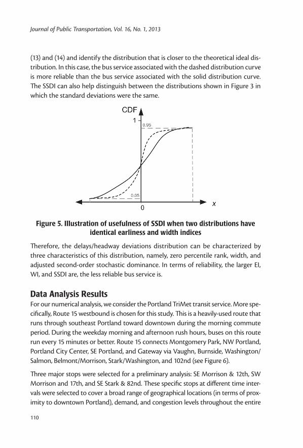
Journal of Public Transportation, Vol. 16, No. 1, 2013
110
(13) and (14) and identify the distribution that is closer to the theoretical ideal dis-tribution. In this case, the bus service associated with the dashed distribution curve is more reliable than the bus service associated with the solid distribution curve. The SSDI can also help distinguish between the distributions shown in Figure 3 in which the standard deviations were the same.
Figure 5. Illustration of usefulness of SSDI when two distributions have identical earliness and width indices
Therefore, the delays/headway deviations distribution can be characterized by three characteristics of this distribution, namely, zero percentile rank, width, and adjusted second-order stochastic dominance. In terms of reliability, the larger EI, WI, and SSDI are, the less reliable bus service is.
Data Analysis ResultsFor our numerical analysis, we consider the Portland TriMet transit service. More spe-cifically, Route 15 westbound is chosen for this study. This is a heavily-used route that runs through southeast Portland toward downtown during the morning commute period. During the weekday morning and afternoon rush hours, buses on this route run every 15 minutes or better. Route 15 connects Montgomery Park, NW Portland, Portland City Center, SE Portland, and Gateway via Vaughn, Burnside, Washington/Salmon, Belmont/Morrison, Stark/Washington, and 102nd (see Figure 6).
Three major stops were selected for a preliminary analysis: SE Morrison & 12th, SW Morrison and 17th, and SE Stark & 82nd. These specific stops at different time inter-vals were selected to cover a broad range of geographical locations (in terms of prox-imity to downtown Portland), demand, and congestion levels throughout the entire

Definition and Properties of Alternative Bus Service Reliability Measures at the Stop Level
111
Sour
ce: F
eng
and
Figl
iozz
i 201
1
Figu
re 6
. Rou
te 1
5 m
ap

Journal of Public Transportation, Vol. 16, No. 1, 2013
112
route. Archived BDS data for Route 15 from 11/30/2009 to 5/23/2010 including more than 115 weekdays were used. For the selected stops, general descriptive statistics along with the TCQSM reliability measures were computed, as shown in Table 1. The TCQSM reliability measure, including on-time performance and headway adherence, were used to determine the LOS at the selected stops. As can be seen, the SW Mor-rison & 17th (2-3 PM) and SE Stark & 82nd (9–10 AM) stops had an LOS of F for their infrequent services while the SW Morrison & 17th (9–10 AM) stop had an LOS of E and the SE Morrison & 12th (6–7 AM) stop had an LOS of A for their frequent services.
Current reliability measures do not tell the whole story of the service reliability. To improve the service reliability, transit agencies should know more than just the percentage of buses that are considered “on-time” and the coefficient of variation of headway deviations. The consequences of late buses may be much different than those of early buses. More information, such as how late or early buses arrive at the stop or how much they are ahead or behind the schedule, is needed to effec-tively improve schedules and operations strategies. Therefore, we recommend that additional measures, such as those presented in this paper, be used as guidance in discussions of reliability.
Table 1. Descriptive Statistics and TCQSM Reliability Measures for the Selected Stops
Service Stop TimeTotal
Number of Trips
Average Scheduled Headway
(sec)
Average Headway Deviation
(sec)
Stdv. of Headway Deviation
(sec)
Headway Adherence
LOS
Frequent
SW Morrison
& 17th
9–10 AM
917 403 5.27 241.69 0.60 E
SE Morrison
& 12th
6–7 AM
509 600 -8.76 124.12 0.21 A
Stop TimeNumber of Trips
Average Scheduled Headway
(sec)
Average Delay (sec)
Stdv. of Delay (sec)
On-time Perfor-mance
LOS
Not Frequent
SW Morrison
& 17th
2-3 PM
404 2100 318.64 264.90 0.53 F
SE Stark & 82nd
9–10 AM
603 735 80.33 145.98 0.63 F

Definition and Properties of Alternative Bus Service Reliability Measures at the Stop Level
113
We carried out an empirical analysis to assess the proposed reliability measures EI, WI, and SSDI for the same selected stops and time periods of Route 15, as shown in Table 1. For frequent services, delay distribution was used and for less frequent (or infrequent) services, headway deviation distribution was used as described in the previous sections.
Figure 7 shows the cumulative distributions of delays and headway deviations for frequent and infrequent service at the selected stops and time periods.
Figure 7. Cumulative distributions of delays and headway deviations for frequent and not frequent services at selected stops
and time periods of Route 15

Journal of Public Transportation, Vol. 16, No. 1, 2013
114
The cumulative distributions of headway deviations shown in Figures 7(a) and 7(b) represent the studied frequent service at SW Morrison and 17th (9–10 AM) and SW Morrison and 12th (6–7 AM) stops. The cumulative distributions of delays shown in Figures 7(c) and 7(d) represent the studied less-frequent service at SW Morrison and 17th (2–3 PM) and SE Stark and 82nd (9–10 AM) stops. Note that TriMet allows its buses to depart up to one minute ahead of schedule. This may explain a large portion of the 30 percent that are not on-time due to early depar-tures at the SE Stark and 82nd (9–10 AM) stop.
As an illustration, Table 2 summarizes the computed reliability measures EI, WI, and SSDI associated with each service at each stop along with its headway adherence and on-time performance. The EI for the less frequent service at SW Morrison and 17th is as low as 0.04, while the EI at SE Morrison and 12th is as large as 0.54. In other words, only four percent of buses at SW Morrison and 17th depart early between 2–3 PM, while 54 percent of buses depart early at SE Morrison and 12th between 6–7 AM. Also, the bus service at SW Morrison and 17th has a WI as large as 1.83 between 9–10 AM, while the WI at the same stop between 2–3 PM is only 0.39. This clearly shows the changing pattern of service reliability in different times of the day. Similarly, the service at SW Morrison and 17th between 9–10 AM has the largest SSDI compared to the other studied services. Note that the SSDI at SW Morrison and 17th reduces from 0.8 between 9–10 AM to 0.15 between 2–3 PM. Overall, the service at SE Morrison and 12th at between 6–7 AM has the worst reliability in terms of EI and SW Morrison and 17th between 9–10 AM has the worst reliability in terms of WI and SSDI.
Table 2. New Reliability Measures at Stop Level
Service Stop Time EI WI SSDIOn-time
PerformanceHeadway
Adherence
FrequentSW Morrison & 17th 9–10 AM 0.5 1.83 0.80 - 0.60
SE Morrison & 12th 6–7 AM 0.54 0.67 0.15 - 0.21
Not Frequent
SW Morrison & 17th 2–3 PM 0.04 0.39 0.15 0.63 -
SE Stark & 82nd 9–10 AM 0.32 0.46 0.14 0.53 -
To further explore the applicability of the proposed measures in the real world, a more comprehensive analysis was carried out using the same archived BDS data for Route 15 westbound including more than 115 weekdays for 11 AM to 12 PM. The new reli-ability measures are applied to the whole route to highlight stops that are candidates for operational improvements such as implementing holding strategy, expressing, schedule adjustment, and re-routing. Figure 8 provides a comparison of the proposed

Definition and Properties of Alternative Bus Service Reliability Measures at the Stop Level
115
reliability measures with headway adherence at each stop, without differentiating between the cost of being early versus late. Note that travel direction is from Gateway Transit Center to NW 23rd & Lovejoy stop. The last two stops were removed from our analysis due to their geometry, which is inconsistent with the rest of the route.
Figure 8. Comparison of (a) Earliness Index; (b) Width Index; and (c) Second Order Stochastic Dominance Index with headway adherence
for Route 15 westbound (travel direction from right to left)

Journal of Public Transportation, Vol. 16, No. 1, 2013
116
The stops with the highest (worst) EI are SE Belmont & 39th and SE Belmont & 60th. Figure 8(a) suggests that there is no correlation between the EI and headway adherence. Also, as shown in Figure 8(b), the stops with the highest (worst) WI are NW 23rd & Lovejoy and SW Morrison & 17th. The WI is following a clear trend throughout the route. As one would expect, the variability of headway adherences are increasing as they move toward the end of the route. This implies the existence of a correlation between consecutive stops in a route. Similarly, the stops with the highest (worst) SSDI are NW 23rd & Love Joy and SW Morrison & 17th. However, the trend in SSDI is not as clear until the middle of the route, where SSDI starts increasing constantly as it moves toward the end of the route.
In this study, an overall consistency was observed among the WI, SSDI, and head-way adherence, as expected. To eliminate the impacts of the existing correlation between consecutive stops along the route and quantitatively demonstrate the dif-ference between the proposed measures and headway adherence, a further analy-sis was performed. Figure 9 shows the percentages of relative difference of selected measures between consecutive stops. The graph shows that SSDI, WI, and headway adherence are capturing different levels of unreliability at each stop relative to its previous stop, despite the general consistency among them. For example, at SE Morrison and 12th (relative to SE Belmont and 60th), the SSDI captures more unre-liability compared to WI and headway adherence, while at SE 102nd & Washington (relative to SE Belmont and 60th), the SSDI captures less unreliability compared to WI and headway adherence. To verify this, further research using data from other routes and time periods is required to study situations where unexpected consis-tency or inconsistency of the proposed measures arises.
Figure 10 illustrates how the EI and On-Time Performance provide different images of service reliability. As shown, On-Time Performance decreases as it moves toward the end of the route, whereas the EI does not follow a specific trend. As explained earlier, arrivals no more than five minutes after the scheduled time and no more than one minute early are considered on-time based on the TCQSM definition, whereas the EI highlights the service unreliability due to the early buses only.
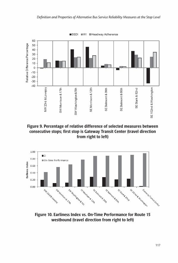
Definition and Properties of Alternative Bus Service Reliability Measures at the Stop Level
117
Figure 9. Percentage of relative difference of selected measures between consecutive stops; first stop is Gateway Transit Center (travel direction
from right to left)
Figure 10. Earliness Index vs. On-Time Performance for Route 15 westbound (travel direction from right to left)

Journal of Public Transportation, Vol. 16, No. 1, 2013
118
Conclusion and Future ResearchThis paper evaluated current measures of bus service reliability, specifically the current TCQSM measures, and developed alternative reliability measures at the stop level. Note that the proposed reliability measures are not suggested as replacements for the existing measures; rather, they are complementary. We inves-tigated the distribution of delays and headway deviations on the basis of empirical archived BDS data from Route 15 in Portland, Oregon, for more than 115 weekdays in 2009–10. Findings are summarized below:
For frequent services, the distribution of headway deviations can be used to mea-sure the percentage of buses that are ahead of the schedule or early. For infrequent services, the distribution of delays should be used. The Earliness Index is proposed.
The distribution of delays/headway deviations is often wide. Commonly-proposed reliability measures in the TCQSM only use the standard deviation and do not take into consideration the full width of this distribution. Also, existing measures do not differentiate between the cost of being early versus late. The Width Index is proposed to capture more of the extreme cases of unreliability and differentiate between the costs of being early versus late.
To further capture characteristics of the distribution of delays/ headway deviations, the concept of second order stochastic dominance is used. As a result, second order stochastic dominance index is proposed. This index is particularly useful when two or more distributions have similar width but different earliness indices. It is also useful to differentiate between distributions with similar width and similar earliness index but with a different curvature that represents different unreliability characteristics.
It was found for the studied route and time period that the Width Index and coef-ficient of variation (or headway adherence) were fairly consistent, whereas the second order stochastic dominance index captured more unreliability in some cases. The Earliness Index provides reliability information that the coefficient of variation does not capture. Eliminating the impacts of the existing correlation between consecutive stops along the route, the difference between the proposed measures and coefficient of variation are quantitatively demonstrated. To further verify the findings and study the situations where consistency or discrepancy of the proposed measures arises, more research using data from other routes and time periods is required.

Definition and Properties of Alternative Bus Service Reliability Measures at the Stop Level
119
Transit agencies can use the proposed reliability measures to evaluate and priori-tize stops for operational improvement purposes, such as bus holdings or schedule adjustments. This paper exhibits how reliability can vary across stops and how important this variation is in prioritizing stops for improvements. A key topic for future research is defining LOS thresholds for bus service reliability. Furthermore, studying the characteristics of the distribution of delays and headway deviations using more data at stop, route, and network level is required to gain more knowl-edge of transit service reliability. Causes of service unreliability are also important to investigate.
Acknowledgments
The authors gratefully acknowledge the contributions of Josh Crain from DKS Associates and Charlotte Frei and Madison Fitzpatrick from Northwestern Uni-versity for their review and feedback. The authors also acknowledge the TriMet and PORTAL team at Portland State University for providing the data. The authors would like to thank Stefan Voss and the anonymous reviewers for their valuable comments and suggestions to improve the quality of the paper.
References
Abkowitz, M., H. Slavin, R. Waksam, L. Englisher, and N. Wilson. 1978. Transit service reliability. TSC Urban and Regional Research Series, U.S. Department of Trans-portation, Cambridge.
Ap. Sorratini, J., R. Liu, and S. Sinha. 2008. assessing bus transport reliability using micro-simulation. Transportation Planning and Technology 31(3): 303–324.
Bellei, G., and K. Gkoumas. 2010. Transit vehicles’ headway distribution and service irregularity. Public Transport 2(4): 269–289.
Bertini, R. L., and A. El-Geneidy. 2003. Generating transit performance measures with archived data. Transportation Research Record 1841: 109–119.
Bertini, R. L., and A. El-Geneidy. 2004. Modeling transit trip time using archived bus dispatch system data. Journal of Transportation Engineering 130(1): 56–67.
Bowman, L. A., and M. A. Turnquist. 1981. Service frequency, schedule reliability and passenger wait times at transit stops. Transportation Research Part A 15(6): 465–471.

Journal of Public Transportation, Vol. 16, No. 1, 2013
120
Camus, R., G. Longo, and C. Macorini. 2005. Estimation of transit reliability level-of-service based on automatic vehicle location data. Transportation Research Record 1927: 277–286.
Chen, X., L. Yu, Y. Zhang, and J. Guo. 2009. Analyzing urban bus service reliability at the stop level, route, and network levels. Transportation Research Part A 43: 722–734.
Duarte, A., C. Garcia, G. Giannarakis, S. Limão, A. Polydoropoulou, and N. Litinas. 2010. New approaches in transportation planning: Happiness and transport economics. Netnomics 11: 5–32.
El-Geneidy, A., J. Horning, and K. Krizek. 2010. Analyzing transit service reliabil-ity using detailed data from automatic vehicular locator systems. Journal of Advanced Transportation 45(1): 66–79.
Feng, W., and M. A. Figliozzi. 2011. Using archived AVL/APC bus data to identify spatial-temporal causes of bus bunching. Proceedings of the 90th Transporta-tion Research Board Annual Meeting, Washington, D.C.
Fu, L., and X. Yaping. 2007. A new performance index for evaluating transit quality of service. Journal of Public Transportation 10(3): 47–70.
Furth, P., B. Hemily, T. Muller, and J. Strathman. 2003. Uses of archived AVL-APC data to improve transit performance and management: Review and potential. TCRP Web Document No. H-28, Washington, D.C.: Transportation Research Board.
Furth, P., and T. Muller. (2006. Service reliability and hidden waiting time: Insights from automatic vehicle location data. Transportation Research Record 1955: 79-87.
Highlights of the Transit Capacity & Quality of Service Manual: 1st Edition (Kittleson & Associates, Inc.) 1999. Research Result Digest, Transit Cooperative Research Program.
Highway Capacity Manual. 2000. Transportation Research Board.
Highway Capacity Manual. 2010. Transportation Research Board.
Kepaptsoglou, K., and M. G. Karlaftis. 2009. The bus bridging problem in metro operations: Conceptual framework, models and algorithms. Public Transport 1: 275–297.

Definition and Properties of Alternative Bus Service Reliability Measures at the Stop Level
121
Kimpel, T. J. 2001. Time point-level analysis of transit service reliability and passen-ger demand. Ph.D. dissertation, Portland State University.
Lin, J., P. Wang, and D. T. Barnum. 2008. A quality control framework for bus sched-ule reliability. Transportation Research Part E 44: 1086–1098.
Transit Capacity and Quality of Service Manual, Second Edition. 2004. Transporta-tion Research Board.
Tumlin, J., J. Walker, J. Hoffman, and R. Hutabarat. 2005. Performance measures for the urban village transit network. Proceedings of the 84th Transportation Research Board Annual Meeting, Washington, D.C.
Van Oort, N., J. W. Boterman, and R. Van Nes. 2012. The impact of scheduling on service reliability: Trip-time determination and holding points in long-headway services. Public Transport 4(1) 39-56.
Xin, Y., L. Fu, and F. Saccomanno. 2005. assessing transit level of service along travel corridors using TCQSM—A case study. Proceedings of the 84th Transportation Research Board Annual Meeting, Washington, D.C.
About the Authors
Meead Saberi ([email protected]) is a Ph.D. candidate in Transporta-tion Systems Analysis and Planning at Northwestern University, Evanston, IL. He received his M.S. degree in Transportation Engineering at Portland State University, Portland, OR. His main research interests are traffic flow theory and characteristics, urban network modeling, transportation data management, and public transit.
Ali Zockaie K. ([email protected]) is a Ph.D. candidate in Trans-portation Systems Analysis and Planning at Northwestern University, Evanston, IL. He received his M.S. degree in Transportation Engineering at Sharif University of Technology, Tehran, Iran. His main research focus is on network modeling and reliability, specifically dynamic network assignment of travelers with heterogeneous risk preferences. His other research interests include public transit, network traffic theory, and airline operations.
Wei Feng ([email protected]) is a Ph.D. candidate in Transportation Engineering at Portland State University, Portland, OR. He received his M.S. degree in Transporta-tion Engineering at Beijing Jiaotong University, Beijing, China. His research interests

Journal of Public Transportation, Vol. 16, No. 1, 2013
122
include traffic flow theory and characteristics, transportation operations, intelligent transportation systems, public transportation, and freight transportation.
Ahmed El-Geneidy ([email protected]) is an associate professor at the School of Urban Planning, McGill University. Ahmed's research interests include land use and transportation planning, transit operations and planning, travel behavior analysis including using motorized and non-motorized modes of transportation, and measurements of accessibility and mobility in urban contexts. Ahmed has a special interest in transportation needs of disadvantaged populations. He received B.S. and M.S. degrees from the Department of Architectural Engineering at Alexandria University, Egypt, and continued his academic work at Portland State University, where he received a Graduate GIS Certificate and earned a Ph.D. in Urban Studies from Nohad A. Toulan School of Urban Studies and Planning. After finishing his Ph.D. he moved to the Twin Cities to work as a post-doctoral research fellow at the University of Minnesota. In 2007 Ahmed moved to Montreal, Canada to start his current position at the School of Urban Planning, McGill University.

123
Maintaining Key Services While Retaining Core Values
Maintaining Key Services While Retaining Core Values: NYC Transit’s
Environmental Justice StrategiesTed Wang, Alex Lu, Alla Reddy
MTA New York City Transit
Abstract
In a recession, transit agencies aim to provide key services while retaining national core values. When making service changes, federal funding recipients are prohibited from discriminating on the basis of race, color, or national origin and must not place undue burden on Environmental Justice (EJ) populations. To ensure compliance, New York City Transit developed analytical methodologies to identify impacts for the 50 proposed service rationalization initiatives, allowing for proactive mitigation. For 38 routes with span changes, load factor analysis across demographic and income categories (during periods of service elimination) demonstrated that impacts were equitably shared. For route changes, impacts were measured using shortest-path trip time and cost analysis using Census Transportation Planning Package Journey-to-Work data. The “M” and “V” Train modifications and the Co-op City bus restruc-turing illustrate package analysis of complex service changes, capturing mitigating effects of adjacent route restructurings. These service changes reduced costs while ensuring that Title VI/EJ communities were not disproportionately affected. After extensive EJ work and community outreach, the proposed changes were imple-mented in June 2010.

Journal of Public Transportation, Vol. 16, No. 1, 2013
124
IntroductionFinding millions of dollars worth of savings in a public transit authority requires shared sacrifice among stakeholders. In 2010, the financial outlook for New York State was deteriorating. Taxes and levies that subsidize New York City Transit (NYCT) fell substantially short of projections. State government was cutting service, and transit needed to do the same to remain solvent. The goal was to keep key public services functioning while seeking budgetary savings. At the same time, the Federal Transit Administration (FTA) requires that funding recipients to comply with Title VI of the Civil Rights Act 1964, ensuring level and quality of service without regard to race, color, and nationality. Executive Order 12898 requires funding recipients to identify and address, as appropriate, disproportionately high and adverse human health and environmental effects, including social and economic effects of programs and activi-ties on minority populations and low income populations (FTA Circular 4702.1A).
FTA provides guidance to transit operators on methods of compliance and allows room for flexibility. It is the operator’s responsibility to develop its own Title VI and Environmental Justice (EJ) programs that comply with FTA and any local standards set by the agency. At the time of this writing, EJ issues are at the forefront of fed-eral rulemaking, as FTA has released two proposed circulars (Circulars 4702.1B and 4703.1) for public comment. The proposals separate Title VI and EJ considerations and reiterate the requirements for service and fare change analysis. There are understandably widespread concerns within the transit practitioner’s community.
This paper demonstrates methods used at NYCT and may serve as an example for other properties concerned with federal compliance when changing route and service span. The purpose of these changes is to seek long-term budgetary savings while minimizing the impact on the community and to safeguard federal funding by remaining in compliance with Title VI and Executive Order 12898. This was achieved through analytical methods detailed in this paper. The service changes discussed in this paper were implemented in June 2010.
Strategic Elements of EJ/Title VITitle VI analysis is also a useful gauge on community relations. Being a good social steward brings positive attention to a business during a difficult time. Transporta-tion infrastructure directly affects job access, property values, and livelihoods. Transit executives need to know the impacts of their decisions.
This information shows its worth when government officials and elected leaders invite transit executives to address concerns of their constituencies. The Oakland

125
Maintaining Key Services While Retaining Core Values
Airport Connector project raised concerns of three San Francisco community groups; they brought the issue to FTA (Thomas and McDaniel 2011), and in 2009, the operator was found to be in violation of Title VI and lost $50 million in federal funding. Ensuring that actions taken by the transit operator are non-discriminatory requires proactive data analysis because outside groups are likely doing this already to influence the outcome. In 1996, Los Angeles County was required by a federal court decision to spend more than $1 billion dollars on its bus system when external groups proved investments on light rail in wealthy neighborhoods were dispropor-tionate compared to the bus network used by the majority of its customers (Garcia 2011). Proactive strategic analysis, therefore, allows operators to take the initiative in matters of decision making, public relations, funding, and control of finances.
Complying with Title VI and Environmental Justice requirements is the law, as well as the right thing to do. However, having first and foremost fulfilled the legal and moral imperatives, taking a proactive approach to Title VI provides the additional benefit of helping to maintain open channels of communication and a good work-ing relationship with community stakeholders and regulators alike. Having a track record of going above and beyond builds an understanding that the operator is well-managed. Satisfying stakeholders consistently indicates that the operator is on the right track in service delivery.
Literature ReviewA literature search for different strategies and analyses yielded a diversity of topics. Some of these reports are unique, such as the analysis done on American Indian tribal territories and transportation in relations to housing and demographics (Ward 2005). One paper described how a transit agency was found to be non-compliant with Title VI and strived to become compliant once again by reviewing the strategies of other operators (Bender et al. 2007). Another paper profiles a list of legal complaints pertaining to alleged Title VI violations (Thomas 2007). Others are more holistic, covering fare analysis, Americans with Disabilities Act (ADA) compliance, and Civil Rights. Recent papers use statistical significance testing to analyze Title VI data (Reddy et al. 2010). This is a logical development since it was already done in many areas: quality control, industrial engineering, and the social sciences, such as crime data mining. Many agencies at the New York Metropolitan Transportation Authority (MTA) have adopted this method of analysis. The con-tribution of NYCT’s experience in 2010 provides focus on a particular case study where a large transit operator faced a financial situation and navigated itself to a fiscally-stronger position using detailed internal analysis as a guide.

Journal of Public Transportation, Vol. 16, No. 1, 2013
126
BackgroundIn 2005, the MTA reduced fares by half for all riders during the holiday season to share with the public an unexpected budgetary surplus. Towards the end of 2007, the world economy entered a recession. Unemployment rose close to 10 percent (New York State Department of Labor 2011). Nationally, those numbers were higher for minority (Holt 2009) and young workers, especially for those with no college degree and even worse for those without a high school diploma (U.S. Department of Labor 2011). Gas prices remained historically high and had made their way past $4 per gallon. Transit provided an alternative means of coping with the cost of auto operation.
Transit also had funding challenges, due to falling tax revenues and rising costs of resources such as fuel and labor. In October 2010, the MTA Board approved fare increases and service reductions for 2011. Title VI analysis found that monthly MetroCard holders tended to be more affluent than other fare media users (Hickey et al. 2010). The decision was to minimize impact on customers least able to pay. An $89 monthly unlimited pass increased to $104; weekly passes increased from $27 to $29; single rides increased by 25 cents to $2.25. Service changes were made to reflect ridership and return on investment. Before any route was discontinued, impact analyses were done to minimize, mitigate, or offset negative effects towards all transit users, especially minority and low-income riders.
Mass transit plays a vital role to those least able to afford private automobiles. Main-taining private auto ownership can cost close to $15,000 annually in New York City (APTA 2011). “At or Below Poverty” is defined as a yearly income of $22,350 for a fam-ily of four and $10,890 for an individual (U.S. Dept. of Health and Human Services 2011). The poverty rate in New York City hovers around 20 percent (Roberts 2010). Despite fare increases, the average annual cost to use transit is a fraction of auto-mobile ownership and can mean the difference between making ends meet or not.
Selection of Analytical TechniquesThere were 50 service rationalization initiatives in 2010. According to guidelines adopted by the MTA in 1988, analysis was not needed if changes are less than 25 per-cent of the net route miles or less than 1 hour of the service span. A total of 14 initia-tives out of the 50 did not surpass thresholds that would require a Title VI Analysis. The remaining initiatives needed a change analysis for route or span. Table 1 shows a selection of initiatives and affected segments and their corresponding analysis types (Span or Route). It was not applicable (N/A) if Title VI analysis was not required.

127
Maintaining Key Services While Retaining Core Values
Table 1. Type of Analysis for Sample List of Services to be Modified
Route SegmentRoute
or Span
% Net Change
Above 25%? Notes
“Q”“N”“W”
Queens ExtensionManhattan LocalAll
RouteN/A
Route
+320
–100
YesNoYes
Extend to AstoriaReplace “W” in NorthEliminated
“V”“M”
Queens EliminationQueens ExtensionBrooklyn Elimination
RouteRouteN/A
–100+71–62
YesYesYes
EliminatedRerouted to replace “V”Discontinued south of Delancey-Essex
“G” Queens EliminationBrooklyn Extension
RouteN/A
–51+14
YesNo
Discontinued East of Court Sq.24hr operation South of Court Sq.
SIR Stadium Service N/A –100 Yes Not a regularly scheduled service
BX25BX26BX28BX30BX38
Co-op CityCo-op CityCo-op CityCo-op CityCo-op City
RouteRouteRouteRouteRoute
–100–33–29–3
+100
YesYesYesNoYes
EliminationRerouted Rerouted
New route
BX55 BX15
BronxBronx
N/AN/A
–23+8
NoNo
BX20 Bronx Span –63 Yes
B1B8B64B70
BrooklynBrooklynBrooklynBrooklyn
RouteRouteRouteRoute
–21–15+41+31
NoNoYesYes
B4 Coney Island Av. East N/A –17 No Modified to operate via Avenue Z
B2B24
BrooklynBrooklyn
SpanSpan
–28–30
YesYes
Weekend discontinuedWeekend discontinued
M22 West of City HallN/A 0 No
Changes recinded due to public hearing
M8M50
ManhattanManhattan
SpanSpan
–32–51
YesYes
Weekend discontinuedWeekend discontinued
S40/90 Staten Island N/A –5 No Discontinued to Howland Hook
S54S76
Staten IslandStaten Island
SpanSpan
–250
YesNo
Q74Q75Q79
QueensQueensQueens
SpanSpanSpan
–100–100–100
YesYesYes
EliminatedEliminatedEliminated
X6 Hylan Blvd Route –100 Yes Express Bus X6 eliminated

Journal of Public Transportation, Vol. 16, No. 1, 2013
128
Span Change AnalysisIt is efficient to reduce bus in-service hours when few people are riding. The follow-ing formula is used to determine number of seats occupied:
Load Factor = (Average Riders / Trip) / Bus Seats
Standard buses have 40 seats and articulated buses have 62 seats. A load factor of 20 percent on a standard bus means that, on average, only 8 seats are occupied at the peak load point during a span of time. A span change analysis is conducted when proposed cuts to service are considered “major,” defined as exceeding more than 1 hour.
Three different span reduction actions were proposed in 2010: (a) span reduction by hour—up to two hours of service at the beginning or end of the day, (b) over-night service elimination (1:00–5:00 AM), and (c) off-peak and weekend service elimination—service may be reduced to weekdays or to peak hours only.
Equitability of span reduction is determined by comparing load factors during the period proposed for span reduction on impacted routes classified for Title VI as Minority or Non-Minority and for EJ as At or Below Poverty (Low Income), or Above Poverty (High Income). A route is defined as Minority if at least one-third of its total route mileage is in a Minority Census tract. The ⅓ rule was first pro-mulgated in Urban Mass Transportation Administration Circular C4702.1 (UMTA 1988) and was retained by NYCT despite the current FTA Circular C4702.1A that allowed each entity to develop local standards. This ⅓ rule is also used to define “At or Below Poverty” routes. One can conclude from Table 2 that the routes selected for span reduction are low performing and sensible candidates for rationalization.

129
Maintaining Key Services While Retaining Core Values
Table 2. Bus Routes Analyzed for Service Span Reduction – Load Factor Analysis
(a) Span Reduction by Hour
Non-Minority Minority
Route Day Type Loads*/ Trip Load Factor Route Day Type Loads*/ Trip Load Factor
B64 ALL 4 10% BX34 ALL 3 8%
B67 ALL 3 7% BX32 WKD 12 29%
B2 WKD 4 10% BX33 WKD 4 11%
B9 WKD 4 10% BX33 SAT 7 18%
B16 WKD 6 15% BX33 SUN 6 15%
B9 SAT 4 9% BX17 SUN 5 12%
B9 SUN 3 8% B7 ALL 6 14%
B16 SUN 3 8% B31 ALL 3 7%
M8 ALL 1 3% B45 ALL 4 10%
M16 ALL 3 6% B57 ALL 6 15%
M50 ALL 2 6% B65 ALL 5 13%
M66 ALL 2 5% B11 WKD 4 10%
M11 WKD 7 18% B13 WKD 4 9%
M20 WKD 6 16% B24 WKD 10 24%
M21 WKD 8 20% M1 ALL 2 6%
M20 SAT 6 15% M22 ALL 1 3%
Q30 ALL 3 9% M22 SAT 3 8%
S54 WKD 4 11% M22 SUN 2 6%
S57 WKD 5 13% M100 SAT 6 14%
S66 WKD 12 29% M116 SAT 7 16%
S57 SAT 3 7% Q48 SUN 3 7%
S57 SUN 4 9%

Journal of Public Transportation, Vol. 16, No. 1, 2013
130
Table 2 (cont'd.). Bus Routes Analyzed for Service Span Reduction – Load Factor Analysis
(b) Overnight Service Elimination
Above Poverty At or Below Poverty
Route Day Type Loads*/ Trip Load Factor Route Day Type Loads*/ Trip Load Factor
B2 WKD 4 10% B9 WKD 4 10%
M8 ALL 1 3% B16 WKD 6 15%
M50 ALL 2 6% B9 SAT 4 9%
M66 ALL 2 5% B9 SUN 3 8%
M20 WKD 6 16% B16 SUN 3 8%
M20 SAT 6 15% M16 ALL 3 6%
Q30 ALL 3 9% M11 WKD 7 18%
S54 WKD 4 11% M21 WKD 8 20%
S57 WKD 5 13% BX34 ALL 3 8%
S66 WKD 12 29% BX32 WKD 12 29%
S57 SAT 3 7% BX33 WKD 4 11%
S57 SUN 4 9% BX33 SAT 7 18%
B31 ALL 3 7% BX33 SUN 6 15%
M1 ALL 2 6% BX17 SUN 5 12%
Q48 SUN 3 7% B7 ALL 6 14%
B45 ALL 4 10%
B57 ALL 6 15%
B65 ALL 5 13%
B11 WKD 4 10%
B13 WKD 4 9%
B24 WKD 10 24%
M22 ALL 1 3%
M22 SAT 3 8%
M22 SUN 2 6%
M100 SAT 6 14%
M116 SAT 7 16%

131
Maintaining Key Services While Retaining Core Values
Tabl
e 2
(con
t'd.).
Bus
Rou
tes
Ana
lyze
d fo
r Se
rvic
e Sp
an R
educ
tion
–
Load
Fac
tor
Ana
lysi
s
(c) W
eeke
nd &
Off
Peak
Ser
vice
Elim
inat
ion
Non
-Min
orit
yM
inor
ity
Abo
ve P
over
tyA
t or B
elow
Pov
erty
Rout
eD
ay
Type
AFC
Lo
ads/
Tr
ip
Load
Fa
ctor
Rout
eD
ay
Type
AFC
Lo
ads/
Tr
ip
Load
Fa
ctor
Rout
eD
ay
Type
AFC
Lo
ads/
Tr
ip
Load
Fa
ctor
Rout
eD
ay
Type
AFC
Lo
ads/
Tr
ip
Load
Fa
ctor
B2SA
T12
31%
BX20
SAT
1332
%B2
SAT
1231
%BX
20SA
T13
32%
B2SU
N9
23%
BX20
OFF
PE
AK
1538
%B2
SUN
923
%BX
20O
FF
PEA
K15
38%
M8
SAT
1129
%BX
34SA
T17
43%
M8
SAT
1129
%BX
34SA
T17
43%
M8
SUN
1024
%BX
34SU
N17
43%
M8
SUN
1024
%BX
34SU
N17
43%
M50
SAT
820
%B2
4SA
T22
55%
M50
SAT
820
%B2
4SA
T22
55%
M50
SUN
616
%B2
4SU
N16
41%
M50
SUN
616
%B2
4SU
N16
41%
Q76
SAT
2870
%Q
26O
FF
PEA
K13
31%
Q76
SAT
2870
%Q
84SA
T19
48%
S54
SAT
1128
%Q
31SA
T31
78%
S54
SAT
1128
%Q
84SU
N16
41%
S54
SUN
820
%Q
31SU
N23
57%
S54
SUN
820
%
S76
SAT
3279
%Q
84SA
T19
48%
S76
SAT
3279
%
S76
SUN
2459
%Q
84SU
N16
41%
S76
SUN
2459
%
Q26
OFF
PE
AK
1331
%
Q31
SAT
3178
%
Q31
SUN
2357
%

Journal of Public Transportation, Vol. 16, No. 1, 2013
132
The average load factors shown Table 3 are less than 50 percent any day of the week for any socio-economic category. That means at least half of the bus seats are empty on weekends, overnight, and the first few hours of service at the beginning of the day and the last few hours at the end. When comparing Minority and Non-Minority on a weekday, the difference in average load factors is 1 percent. The difference between High and Low Income is 2 percent. The t-test shows “No disparity” among these groups. Statistically speaking, the differences between groups are not significant.
Table 3. Comparing Load Factors between Community Groups and Determining Disparity Using t-Tests (Dataset in Table 2)
Title VI Environmental Justice
MinorityNon-
MinorityAt or Below
PovertyAbove
Poverty
Weekday Analysis
Average load factor 12% 11% 12% 10%
Variance 0.0038 0.0036 0.0034 0.0039
t-test -2.02 < -0.60 < 2.02 -2.04 < -1.32 < 2.04
Comparison results No disparity No disparity
Weekend Analysis
Average load factor 46% 36% 43% 40%
Variance 0.018 0.049 0.0046 0.0529
t-test -2.12 < -1.32 < 2.12 -2.11 < -0.34 < 2.11
Comparison results No disparity No disparity
The load factor analysis acts on the systemwide level, with each route being a unit of analysis. This analysis is applicable when many routes are having their service spans reduced and essentially tests to see if span reductions are over-represented among certain routes to detect unintentional discrimination, if any. In contrast, route change analysis, discussed in the next section, is a route-by-route method that focuses on equity within the route, with Census tracts being the unit of analysis.
Subway Route ChangeWorking toward the goal of saving $4 million per annum, planners at NYCT pro-posed eliminating the “V” Train and replacing it with a rerouted and extended “M” Train (Figure 1). The “V” Train had relatively low ridership. The neighborhoods that lost and gained service had parity in demographics; thus, equity was preserved. Public hearings were held and comments were collected in March 2010. The route change offered a new Midtown direct service for riders originating from Middle Village, Ridgewood, and Fresh Pond in Queens and Bushwick and Williamsburg in

133
Maintaining Key Services While Retaining Core Values
Brooklyn. This modification was considered major because it changed at least 25 percent of the “M” Train route length and, thus, required a Title VI analysis (NYCT 1985). The results from an Equity Analysis using a t-test showed that average travel times in affected Minority and Non-Minority areas showed no significant difference.
Figure 1. “M” and “V” train service changes: (a) description from 2010 service reduction proposal, (b) schematic map

Journal of Public Transportation, Vol. 16, No. 1, 2013
134
Figure 1 (cont'd.). “M” and “V” train service changes: (a) description from 2010 service reduction proposal, (b) schematic map

135
Maintaining Key Services While Retaining Core Values
Route Analysis MethodsFor routes that are being modified (eliminated or extended), or those that have greater than 25 percent of total revenue miles being changed, NYCT conducts a travel time and cost analysis. All Census tracts within ¼ mile of the route are reviewed. According to FTA Circular 4702.1A, a “Predominantly Minority Area” is a geographic area such as a neighborhood, Census tract, or traffic analysis zone where the proportion of minority persons residing in that area exceeds the average proportion of minority persons in the recipient’s service area. The 2000 citywide average showed minorities to be 65.02 percent of the population of New York City. Thus, a Census tract in New York City is considered to be “Minority” if the minor-ity population is equal to or greater than 65.02 percent; otherwise, it is defined as “Non-Minority.” A Census tract is considered to be “At or Below Poverty” if the population is equal to or greater than the 2000 citywide average of 21.25 percent; otherwise, it is defined as “Above Poverty.”
Thresholding is a necessary part of binary EJ analysis, where the population is divided into only two categories. Some observers feel it would be simpler or more appropriate to set the boundary at 50 percent, such that if more than half the people in a tract are minority, then the entire tract should be considered minority. However, this is problematic for New York City where minorities make up more than half of the population, resulting in most of the city being classified as minority and giving rise to analysis that would not be sensitive to actual disparities between heavily-minority areas versus somewhat-minority areas. Using the metro area aver-age as the threshold is an appropriate way of ensuring that there is approximately same number of tracts in both categories, thereby maximizing the detection power of the statistical t-tests.
Similarly, defining areas of poverty at 50 percent will dramatically reduce the detec-tion power of the analyses since most tracts will not meet the 50 percent threshold, and impact analysis may never be triggered. FTA provides guidelines on thresholds, and NYCT abides by the current standard practice (FTA C 4702.1A, 2007).
An Origin-Destination (O-D) table was created from the 2000 Census Journey-to-Work Matrix, separately for Minority- and Non-Minority-originating Census tracts. The top five tracts in terms of passenger origination within ¼ mile of the route were selected. From these top five origin tracts, the top three destinations within NYCT’s service area were selected, making a selection of 15 O-D pairs with heavy traffic on NYCT’s services, on which travel time and cost analysis were conducted.

Journal of Public Transportation, Vol. 16, No. 1, 2013
136
1. The shortest path using the route being proposed for elimination is selected as the “before” travel time. The shortest path without the use of that route is the “after” travel time. The shortest path is recommended by a generic Web-based shortest-path journey planning tool.
2. If the shortest path is to walk between the origin and destination Census tracts, the walk time is entered and $0 is entered for the fare.
3. In some cases, it is necessary to find the shortest path by forcing a transfer at an intermediate transfer point, as a trip planner is not always able to pick a path using the route in question. Paths are rejected for being unreasonable if they involve circuitous changes of direction (e.g., travel south on a bus in order to go back north on an express bus.)
4. If there is no way to use the subject route (e.g., the Census tract is at the northern end of the subject route, and the O-D pair requires the traveler to travel north; thus, every path involving the subject route results in a “go south to go north” condition), then the shortest path travel time is used for both the before and after conditions (i.e., elimination of route will have no impact for that O-D pair.)
The travel times and costs are found for each O-D pair before and after route modi-fication. The average difference is calculated. A t-test is conducted to determine if the changes in travel times and cost are equitable.
Application and ResultsThis method was applied to the “M” Train modification from Lower Manhattan to South Brooklyn. Prior to the major revamp of the subway map, the “M” Train from Broad Street in Manhattan to Bay Parkway in Brooklyn was a dotted line, indicating a part-time extension. It ran only during rush hours Monday through Friday from 6:30–9:30 AM and 3:30–8:00 PM. There was no service available during midday, evenings, weekends, and late nights. Between Broad Street in Manhattan and 36th Street in Brooklyn, it shared the Montague Street tubes and 4th Avenue subway local tracks with “R” Trains. Then, it shared the West End Line tracks with “D” Trains as far as Bay Parkway. The redundancy reduced the impact of its elimination. Table 4 illustrates the top five origins and top three destinations for the “M” Train. The results are graphed in Table 5 to show the average difference in travel time and cost affecting four demographic categories before and after the “M” Train was modified.

137
Maintaining Key Services While Retaining Core Values
The bar graph shows the differences before and after the “M” Train modification (“M” Elimination). In terms of average travel times for minorities, there is a frac-tion of a minute difference. The same is true for non-minorities. The comparison is between the average difference of minorities and non-minorities. The change was equitably small. The two-tailed test of hypothesis (t-test) confirms this conclusion of “No Significant Disparity.” Due to the “One City, One Fare” policy, the average difference in total cost per trip between minority and non-minority riders are iden-tical; therefore, there was no Title VI disparity. The average difference for Above Poverty and At or Below Poverty was also insignificant according to t-test results.
The new orange “M” Train (“M” Extension) runs from Broadway/Lafayette Street in Manhattan to Forest Hills in Queens. This extension completely replaces—and thus eliminates in name only—the “V” Train. The neighborhoods the “M” now travels through (all former “V” stops) include a largely non-minority and above-poverty population in Manhattan. Once the “M” Train crosses underneath the East River and enters Queens, the population becomes quite diverse in terms of race and income.
The methodology used to analyze the “M” Extension and the “V” Elimination is based on the route change analysis done on the “M” modification in Lower Manhattan to South Brooklyn. There are geographic differences between the eliminated segment of the “M” Train and the extended portion going into Queens. Brooklyn has higher transit density, providing more options for transfers.

Journal of Public Transportation, Vol. 16, No. 1, 2013
138
Tabl
e 4.
Tit
le V
I—M
inor
ity/
Non
-Min
orit
y A
naly
sis

139
Maintaining Key Services While Retaining Core Values
Tabl
e 4
(con
t'd.).
Tit
le V
I—M
inor
ity/
Non
-Min
orit
y A
naly
sis

Journal of Public Transportation, Vol. 16, No. 1, 2013
140
Tabl
e 4
(con
t'd.).
Tit
le V
I—M
inor
ity/
Non
-Min
orit
y A
naly
sis
Tota
l Tra
vel T
ime:
Usin
g a
two-
taile
d te
st o
f hyp
othe
sis w
ith a
5%
err
or (9
5% c
onfid
ence
), th
e re
sulti
ng t-
stat
istic
= -1
.69.
The
t-cr
itica
l val
ues a
re
+/- 2
.05.
Sin
ce -1
.69
> –2
.05
and
< +2
.05,
we
can
ther
efor
e co
nclu
de th
at th
ere
is no
sign
ifica
nt d
iffer
ence
in th
e to
tal t
rave
l tim
e be
fore
and
aft
er
elim
inat
ing
the
prop
osed
rout
e be
twee
n m
inor
ity a
nd n
on-m
inor
ity p
opul
atio
n.
Tota
l Cos
t per
Tri
p: Th
e av
erag
e di
ffere
nce
in to
tal c
ost p
er tr
ip b
etw
een
min
ority
and
non
-min
ority
ride
rs a
re e
qual
; the
refo
re th
ere
is no
Titl
e V
I di
spar
ity.
Not
e: O
-D c
entr
oid
pairs
com
e fro
m C
ensu
s yea
r 200
0 jo
urne
y-to
-wor
k m
atrix
. Tra
cts a
re a
djac
ent t
o aff
ecte
d ro
utes
. Top
5 o
rigin
s and
top
3 de
stin
atio
ns
are
sele
cted
.

141
Maintaining Key Services While Retaining Core Values
Table 5. Travel Time and Cost Analysis: “M” and “V” Subway Restructuring
Travel Cost Analysis
GroupBefore (Mins.)
After (Mins.)
Avg. Diff. Var. t-Test Result
“M” Elim Minority“M” Elim Non-Minority
5.99.1
5.79.2
-0.20.1
0.30.3
-2.05 < -1.69 < 2.05 No disparity
“V” Elim Minority“V” Elim Non-Minority
15.44.7
15.14.7
-0.3-0.1
0.40.1
-2.09 < -1.54 < 2.09 No disparity
“M” Ext Minority“M” Ext Non-Minority
14.94.7
14.94.7
0.00.0
0.00.0
Not required No change
No disparity
“M” Elim Poverty“M” Elim Non-Poverty
5.710.8
5.510.9
-0.20.1
0.30.3
-2.05 < -1.69 < 2.05 No disparity
“V” Elim Poverty“V” Elim Non-Poverty
14.34.7
16.94.7
2.7-0.1
52.80.1
-2.14 < 1.46 < 2.14 No disparity
“M” Ext Poverty“M” Ext Non-Poverty
14.74.7
14.74.7
0.00.0
0.00.0
Not required No change
No disparity

Journal of Public Transportation, Vol. 16, No. 1, 2013
142
Table 5 (cont'd.). Travel Time and Cost Analysis: “M” and “V” Subway Restructuring
Travel Cost Analysis
Group Before AfterAvg. Diff. Var. t-Test Result
“M” Elim Minority“M” Elim Non-Minority
$0.60$1.00
$0.60$1.00
0¢0¢
0¢0¢
Not RequiredNo Change
No disparity
“V” Elim Minority“V” Elim Non-Minority
$1.23$0.90
$1.33$0.90
10¢0¢
15¢0¢
-2.14 < 1.00 < 2.14 No disparity
“M” Ext Minority“M” Ext Non-Minority
$1.43$0.90
$1.43$0.90
0¢0¢
0¢0¢
Not requiredNo change
No disparity
“M” Elim Poverty“M” Elim Non-Poverty
$0.60$1.00
$0.60$1.00
0¢0¢
0¢0¢
Not requiredNo change
No disparity
“V” Elim Poverty“V” Elim Non-Poverty
$0.90$0.90
$1.77$0.90
87¢0¢
523¢0¢
-2.14 < 1.47 < 2.14 No disparity
“M” Ext Poverty“M” Ext Non-Poverty
$2.20$0.90
$2.20$0.90
0¢0¢
0¢0¢
Not requiredNo change
No disparity
DiscussionThe methodology takes into account people who walk distances up to a quarter mile, and there could be several stops in between. The distance between Allen Street at Delancey Street and Crosby Street at Grand Street is easily 4–5 minutes

143
Maintaining Key Services While Retaining Core Values
walking but has four separate subway stations within its vicinity. The variances in these O-D pair comparisons (Table 4) jump to 52.81 when trips between 31 Avenue at 34th Street in Queens and Stone Street at Broad Street in Manhattan are added. The distance between these two points is approximately 7 miles and requires, at minimum, a transfer between two train routes. The difference in travel time could range from 4 to 44 minutes.
The trip planner method has its limitations, and this could be seen when analysis was done on total cost per trip for the “V” Train elimination. The journey planner generates the top 3–5 shortest travel paths for each given O-D pair. On two occa-sions, it recommended use of the Long Island Rail Road (LIRR)—if no “V” Train were available—to travel between 35th Avenue at 71st Street, Queens and Midtown Manhattan, which is a distance of about five miles. The LIRR is a viable, if not more expensive, mode of transport for that trip. However, the trip planner (at time of analysis) could not take into account the fact that the new “M” Train would replace the “V” Train in its entirety and that, in reality, a subway option continued to be available. The journey planner data cannot be modified until these proposals are adopted and MTA releases appropriate timetable data. One can make an excep-tion, but in this study, the method was strictly followed to ensure that NYCT has a consistent and defensible Title VI/EJ analytical method.
As a result of the “V” Train elimination being analyzed separately from the “M” Train re-route, the methodology makes the data appear that At or Below Poverty riders are paying almost twice as much as Above Poverty riders. In actuality, the fare did not change before or after the elimination of the “V” train. Based on new package analysis methodology submitted for FTA review, NYCT will analyze route changes such as the “M” Train and the “V” Train together in the future.
Bus Service Change: Co-op CityCo-op City is a middle-income housing development located on the northeast peninsula of the Bronx, privately built under New York’s Mitchell-Lama limited-profit housing program. It is not a separate municipal jurisdiction but is the name of a neighborhood that contains a high density of co-operatively-owned apartments situated on attractive parkland with easy access to parking and state parkways but not rail rapid public transit. Nearby amenities include a golf course, a beach, a shopping mall, and a municipal park. Per Census data, this neighborhood is Minority and Above Poverty.

Journal of Public Transportation, Vol. 16, No. 1, 2013
144
Consider the Title VI analysis of restructuring four bus lines in Co-op City. The cessation of an entire bus line (BX25) is projected to save $2.8 million per annum. The other three buses (BX26, BX28, BX38) will be altered to absorb the ridership of BX25: 1) reroute the BX26 to match the eliminated BX25 path at all times (the BX25 designation would no longer be used); 2) split the BX28 into two branches, with one serving the northern section of Co-op City (which would be extended to Bay Plaza and numbered BX38) and one serving the southern section of Co-op City (which would be numbered BX28); and 3) BX38 will not enter Asch Loop. These buses serve as feeders to the “2” and “5” Trains going into Manhattan and Brooklyn; they also go to the Metro-North Williams Bridge commuter rail station.
BX25, BX26, and BX28 are considered Minority bus routes because at least ⅓ of their total route mileage is in Minority Census tracts. These Census tracts are defined as Minority when 65.02 percent or more of their population are minority, per the 2000 New York City minority population threshold. Even though 34.98 percent or less are Non-Minorities, the entire Census tract is considered Minority. Thus, non-minorities do exist there even though the methodology treats these Census tracts as one or the other. Despite the route being predominately minority, the analysis compares the experience of minorities and non-minorities within the route by comparing Census tracts. The income levels are also worth mentioning because Co-op City is well known for being a community of the urban middle class popular among minorities and émigrés. The income requirements to live in Co-op City start at $23,160 for up to two people, which is just above poverty.
The method of analysis to determine Title VI compliance in Co-op City is simi-lar to the “M” and “V” Train modification discussed earlier. The difference is the additional variables of four routes being modified as opposed to just two for the “M” and “V” trains. The graphs on Table 6 show the changes in travel time and cost before and after modification. The average differences among the four socio-economic categories are less than half a minute or zero.

145
Maintaining Key Services While Retaining Core Values
Table 6. Travel Time and Cost Analysis: Co-op City
Travel Cost Analysis
GroupBefore (Mins.)
After (Mins.)
Avg. Diff. Var. t-Test Result
BX25 MinorityBX25 Non-Minority
25.524.1
25.524.1
0.00.0
0.00.0
Not requiredNo change
No disparity
BX26 MinorityBX26 Non-Minority
34.20.0
34.60.0
0.40.0
0.00.0
No comparisonData
No disparity
BX28 MinorityBX28 Non-Minority
34.20.0
34.60.0
0.40.0
0.00.0
No comparisonData
No disparity
BX38 MinorityBX38 Non-Minority
24.526.6
24.526.6
0.00.0
0.00.0
Not requiredNo change
No disparity
BX25 PovertyBX25 Non-Poverty
18.430.6
18.430.6
0.00.0
0.00.0
Not requiredNo change
No disparity
BX26 PovertyBX26 Non-Poverty
0.031.9
0.032.3
0.00.4
0.00.0
No comparisonData
No disparity
BX28 PovertyBX28 Non-Poverty
0.031.9
0.032.3
0.40.4
0.00.0
No comparisonData
No disparity
BX38 PovertyBX38 Non-Poverty
16.929.5
16.929.7
0.00.2
0.00.6
Not requiredNo change
No disparity

Journal of Public Transportation, Vol. 16, No. 1, 2013
146
Table 6 (cont'd.). Travel Time and Cost Analysis: Co-op City
Travel Cost Analysis
Group Before AfterAvg. Diff. Var. t-Test Result
BX25 MinorityBX25 Non-Minority
$1.22$1.32
$1.22$1.32
0¢0¢
0¢0¢
Not requiredNo change
No disparity
BX26 MinorityBX26 Non-Minority
$1.10$0.00
$1.10$0.00
0¢0¢
0¢0¢
No comparisonData
No disparity
BX28 MinorityBX28 Non-Minority
$1.10$0.00
$1.10$0.00
0¢0¢
0¢0¢
No comparisonData
No disparity
BX38 MinorityBX38 Non-Minority
$1.51$1.20
$1.51$1.20
0¢0¢
0¢0¢
Not requiredNo change
No disparity
BX25 PovertyBX25 Non-Poverty
$1.53$1.00
$1.53$1.00
0¢0¢
0¢0¢
Not requiredNo change
No disparity
BX26 PovertyBX26 Non-Poverty
$0.00$1.10
$0.00$1.10
0¢0¢
0¢0¢
No comparisonData
No disparity
BX28 PovertyBX28 Non-Poverty
$0.00$1.10
$0.00$1.10
0¢0¢
0¢0¢
No comparisonData
No disparity
BX38 PovertyBX38 Non-Poverty
$1.02$1.19
$1.02$1.19
0¢0¢
0¢0¢
Not requiredNo change
No disparity

147
Maintaining Key Services While Retaining Core Values
The top five origination method has a notable effect on the analysis. BX25 and BX26 travel along a similar path, but the top five origins for each route fall on different Census tracts. BX25 has data to compare between minorities and non-minorities. BX26 top five origins do not fall on any Non-Minority Census tracts, so there are no data to compare with Minority. BX26 top five origins do not fall on any At or Below Poverty Census tracts either, so there are no data to compare with Above Poverty tracts (Table 6).
Public ReactionThe residents of Co-op City formed a “Coalition to Stop the MTA Cuts” and pre-sented a petition to the MTA and their elected representatives signed by thou-sands. Nine months of meetings among the stakeholders yielded “the relocating of a bus stop from under the I-95 overpass to a better lit location closer to Baychester Avenue. A request to add buses to the BX28 line serving the north section of the community during the overnight hours was accepted” (Stuttig 2011, 22).
Still, a local city council believed the concessions have not gone far enough. He called for the MTA to “return to the drawing board and make sure the residents of Co-op City are not stranded” (Stuttig 2011). Having learned that these cuts saves millions of dollar per year, he claimed that “Co-op City has received an unfair share of the cuts made system-wide and as such should be given some consideration for having some of the previous level of service restored.” FTA auditors may be satis-fied and are assured that the reductions have been necessary and fair. However, NYCT strives to be customer-oriented and has maintained communications and negotiations with community leaders and their constituents. There may be no legal requirement to do so, given the exhaustive Title VI and EJ analysis, but it is a matter of working in good faith with stakeholders. One local media outlet reported that “ridership data will be reviewed to determine if service adjustments need to be made. Bronx residents will be given opportunities to speak out at town hall meet-ings” (News 12 2011).
Package Level Analysis Route level analysis is cumbersome and can be misleading because it does not capture the mitigating effects of restructuring other adjacent routes. A segment of the “M” Train in this study was eliminated in one area of Census tracts that have route redundancy mitigating any impacts to riders there. The “V” Train was elimi-nated, but only in the sense that the designation was no longer used. The Queens Boulevard Line local track that the “V” Train traveled was not physically removed.

Journal of Public Transportation, Vol. 16, No. 1, 2013
148
Riders still have access to train service with a different letter (“M”) and, in some sense, can go further with fewer transfers than before. Yet, analysis of the “V” Elimi-nation absent the “M” makes the result appear to impact one group more (albeit negligibly). Nevertheless, a route change has occurred and, thus, Title VI route level analysis must be done. The following formula summarizes when it is important to conduct an impact analysis as a package of changes.
Above X% Net Route Miles Change =
(New Mileage + Eliminated Mileage) / Σ (Original Route Mileage)
The X% is for each operator to decide. At NYCT, if the X% Net Route Miles Change is greater than 25 percent, then a package analysis should be conducted; no action is required if it is under 25 percent. Future NYCT Title VI analysis involving a com-bination of changes will use the method of package analysis in cases such as Co-op City. This method has been reviewed by FTA auditors and yields results that better represent the experiences of the riding public, not to mention making the analysis process easier.
Figure 2 is a hypothetical package analysis on a series of changes made to four routes. The focus of change is on Route 4 (or R4) because it is being eliminated. The original routes are R3, R4, R5, and R6. The gray horizontal line that makes a right-angle turn is R4 and stretches from segments E, F, G, and H, ending at D. The adjacent R5 is being extended to segment E, covering a portion of the R4 elimina-tion. Segment F would not be covered by any bus route, and riders will have to walk to bridge that distance. The adjacent R6 used to run in a straight line but, in order to cover a little more of the R4 elimination, now has to make a turn to run through segment G before heading south again to segment J. The distance of segment H also will not be covered by any bus route. The final segment to cover is D, which is taken over by extending R3. The modification of bus routes R5, R6, and R3 has now made bus route R4 no longer necessary. The percent of net route change is the quotient produced by the above formula. If the percentage is above 25 percent, then a Title VI analysis will be necessary.
This method of rationalization keeps the network relatively intact, which means people can still get to where they need to go but with some impact in connectivity. A rider may be accustomed to riding R5 to the end and transferring to R4 to get towards G. The transfer would be within the same block. Eliminating R4 means the rider has to walk distance F to catch R6 in order to complete the journey.

149
Maintaining Key Services While Retaining Core Values
% Net Route Change = Length (J+F+H+I) / Length (R3+R4+R5+R6)
Figure 2. Net route change example in a package analysis
ConclusionIt is the dynamic communication with the community and the analysis of the cus-tomer base that ensures the provision of the best level of service with the resources available. This effort makes every dollar count. Proving to the public that the impact on travel time for minorities in Co-op City is minimal frames the grievance they may have about losing an entire bus line and counters anecdotal experiences of poor service. Even if the impact can be measured by minutes, it helps to show that, statistically speaking and as a measure on the whole, the change is equal for minori-

Journal of Public Transportation, Vol. 16, No. 1, 2013
150
ties and non-minorities on that route. The effort and methods invested could save the operator from having to reverse their decisions, which in itself is costly.
Analysis of these issues needs to evolve to meet the needs of the operator and the community. In the case of the “M” and “V” trains, it may have been appropriate to analyze them as one route because the two were designed to be complementary as parts of a package of service changes. Likewise, this method could also be used to conduct surface analysis in Co-op City. Although the restructuring of routes in rapid transit is infrequent, the future of these types of service changes will likely be analyzed as a combined “package” of changes to account for the complex and interlinked nature of such system modifications.
Despite the scientific methods, there is still a qualitative element that operators must heed. Title VI analyses are just tools employed in multi-lateral communica-tion, ensuring that the operator, the riding public, and the government are all “on the same page” in terms of the effects of service changes on the community.
These methods for analyzing service changes are being developed at a time when the federal government is tightening the Title VI and EJ enforcement machinery through more thorough and detailed audits, promulgation of new rules, and requirements of transparency and accountability. FTA has affirmed its position through its proposed circulars, requiring all transit agencies to consider Title VI and EJ in service and fare changes that are becoming increasingly commonplace. Proper application of and further developing the methods discussed in this paper will allow the transit industry to move forward and maintain the balance between providing socially necessary services and upholding fiduciary responsibility. Retain-ing national core values require transit operators to go back to the basics: listening to the customers that it serves.
Acknowledgments
The authors would like to acknowledge the assistance of the following col-leagues during this manuscript’s development: Thomas Chennadu, Anthony Cramer, John Cucarese, Michael Kelly, Santosh Kumar, Brian Levine, and Svetlana Rudenko. Responsibility for errors or omissions remains with the authors. Opinions expressed are those of the authors and do not necessarily reflect official policy of Metropolitan Transportation Authority, MTA New York City Transit, or the Federal Transit Administration.

151
Maintaining Key Services While Retaining Core Values
References
American Public Transportation Association (APTA). 2011. Double digit rise in gas prices marks largest savings in nearly three years, giving public transit rid-ers economic edge. http://www.apta.com/mediacenter/pressreleases/2011/Pages/110414_TSR_april.aspx. Accessed June 1, 2011.
Bender, J., C. Bell, and B. Hill. 2007. Title VI: implementing a transit equity program. DMJM Harris and Maryland Transit Administration.
Garcia, R. Transportation equity in Los Angeles: The MTA and beyond. Environ-mental Defense Fund. http://www.edf.org/article.cfm?contentID=1238. Accessed June 10, 2011.
Hickey, R. L., A. V. Reddy, and A. Lu. 2010. Using quantitative methods in equity and demographic analysis to inform transit fare restructuring decisions. Transpor-tation Research Record, TRB Paper #10-0280.
Holt, A. 2009. Women and people of color down for the count in jobless recovery. Huffington Post, October 13. http://www.huffingtonpost.com/arlene-holt/women-and-people-of-color_b_318672.html Accessed June 1, 2011.
MTA New York City Transit. 1985. MTA guidelines—service change procedures. NYCT Operations Planning Department (Report OP - X85006), June 1.
New York State Department of Labor. 2011. Employed, unemployed, and rate of unemployed by place of residence for New York State and major labor areas. May. http://www.labor.ny.gov/stats/pressreleases/prtbur.txt Accessed June 1, 2011.
News 12. 2011. BX28 riders say cuts are hurting service. News 12 The Bronx, April 19.
Reddy, A. V., T. Chennadu, and A. Lu. 2010. Safeguarding minority civil rights and environmental justice in service delivery and reductions: Case study of New York City Transit Authority Title VI Program. Transportation Research Records 2163, TRB Paper #10-1155.
Roberts, S. 2010. Calculating poverty in New York: More by city standard, and less by federal one. The New York Times, March 2.
Stuttig, B. 2011. Benedetto invites MTA chairman to tour Co-op City. Co-op City Times, March 26.

Journal of Public Transportation, Vol. 16, No. 1, 2013
152
Thomas, L. W., and J. B. McDaniel, J.B. 2011. Reductions in transit service or increases in fares: Civil rights, ADA, regulatory, and environmental justice implications. TCRP Legal Research Digest 35: 13–14.
Thomas, L. W. 2007. Civil rights implications of the allocation of funds between bus and rail. TCRP Legal Research Digest.
U.S. Department of Labor, Bureau of Labor Statistics. 2011. Employment status of the civilian population 25 years and over by educational attainment. http://www.bls.gov/news.release/empsit.t04.htm Accessed June 1, 2011.
Urban Mass Transportation Administration (UMTA). 1988. Title VI Program guide-lines for Urban Mass Transportation Administration recipients. Circular UMTA C4702.1 Section I-3, May 26.
Ward, B. G. 2005. Case Studies in environmental justice and public transit Title VI reporting. National Center for Transit Research, University of South Florida.
About the Authors
Ted Wang ([email protected]) has been a Staff Analyst since 2007 in the Divi-sion of Operations Planning at New York City Transit. He has co-authored published papers on profitability of transit operations and transportation workforce devel-opment. His current research interest is in transportation equity and international best practices. He holds an M.A. in Urban Affairs from Queens College, where he focused his interest and thesis on the political feasibility of Bus Rapid Transit for New York City.
Alex Lu ([email protected]) is a transit analyst with 14 years of experience in transportation research and railroad management in the United States and Great Britain. Currently an employee of a U.S. commuter railroad, his research interest is in strategic planning, international best practice, and decision-support analyses and algorithms. He obtained an M.S.T. from the Massachusetts Institute of Technology.
Alla V. Reddy ([email protected]) is the Senior Director of System Data & Research in New York City Transit’s Division of Operations Planning. He obtained an M.S. in Operations Research from Polytechnic University in Brooklyn in 1976. In his more than 30 years of NYCT experience, he has practiced in the areas of industrial engineering, internal auditing, materials management, performance analysis, and environmental justice. His research interest is in using quantitative research to solve management problems and improve system productivity and efficiency.

153
A Bus Rapid Transit Line Case Study: Istanbul’s Metrobüs System
A Bus Rapid Transit Line Case Study: Istanbul’s Metrobüs System
M. Anıl Yazıcı Region-2 University Transportation Research Center, New York
Herbert S. Levinson, P.E., NAE
Mustafa Ilıcalı
Bahçeşehir University, Istanbul
Nilgün Camkesen Bahçeşehir University, Istanbul
Camille Kamga
City College of New York
Abstract
Implementation of Metrobüs, the first bus rapid transit (BRT) line in Istanbul, Turkey, started in 2007. Since then, the line has been extended several times. After opening of the fourth phase in 2012, the BRT line will extend for 51.3 km. Currently, Metrobüs carries around 600,000 passengers per day. It is the only intercontinental BRT system in the world. This paper describes Istanbul’s Metrobüs system features and usage and its reported benefits and costs. It also gives the reasons that underlie the positive public reception and the rapid ridership increase.

Journal of Public Transportation, Vol. 16, No. 1, 2013
154
IntroductionHigh levels of traffic congestion in urban areas and constrained resources require public agencies to fund timely and effective solutions, preferably with low initial costs. Istanbul’s intercontinental Metrobüs bus rapid transit (BRT) line is one such solution. The line, first opened in 2007 and progressively expanded, carries a large number of riders and has dramatically reduced travel times.
This paper describes the Metrobüs system and identifies the reasons underlying the rapid increase in ridership and public acceptance. It overviews Istanbul’s vari-ous public transportation systems, gives the history and physical features of the Metrobüs project, and sets forth ridership trends, rider demographics, and changes in accessibility and modal shift. The presented analysis is largely based on the data provided by the Istanbul Public Transport Authority (IETT), the Metrobüs opera-tor. It also presents the reported benefits of Metrobüs and the passenger attitudes based on a survey conducted by IETT. The paper then compares Metrobüs features and performance with major BRT lines elsewhere in the world. It concludes with a discussion of the role of Metrobüs in Istanbul’s public transportation system and the reasons underlying its popularity.
Transportation in IstanbulIstanbul is one of the largest cities in the world, with a population of more than 13 million inhabitants, according to the 2010 census (TurkStat 2010). Similar to New York City and other megacities similar in size and complexity, Istanbul’s metropoli-tan area is even larger. The Bosporus Sea channel divides the city into two parts and connects the Black Sea and Mediterranean Sea through the Marmara Sea. It also forms the natural boundary between Europe and Asia. Despite the Bosporus’s posi-tive impact on the city’s landscape and historic development, it concentrates and complicates access within the city. The two sides of Istanbul are connected by two highway bridges (the Bosporus Bridge and the Fatih Sultan Mehmet Bridge) and by maritime transportation (ferries, passenger boats). The demand for maritime transportation is limited since it serves only certain waterfront locations.
The Bosporus Bridge (also known as the First Bridge) was completed in 1973 and became increasingly congested in subsequent years. The Fatih Sultan Mehmet Bridge (the Second Bridge) project started in 1986 and was completed in 1988. The two bridges accommodate only highway vehicles—cars, trucks, and buses. The Marmaray project, an underground rail tunnel, is under construction and, when completed, will also connect the European and Asian sides of Istanbul. At pres-

155
A Bus Rapid Transit Line Case Study: Istanbul’s Metrobüs System
ent, passenger transportation between the residentially-heavy Asian side and the business-oriented European side can use only using the two existing bridges over the Bosporus, which are congested for many hours each day.
Car ownership in Istanbul is lower than in other European cities. It has increased sub-stantially over the last decade, significantly exceeding population growth (Gercek and Demir 2008). The current car ownership rate is 134 cars per 1,000 inhabitants; about 65 percent of households in Istanbul do not have a car (Gercek and Demir 2008).
Transportation in Istanbul mainly relies on road-based transportation (92.3%), followed by rail (5.5%) and water (2.2%) (Gunay 2007). The city’s residents have a strong dependence on the its comprehensive public transportation system. Over-all, 53 percent of the population use one or more forms of public transportation (Gunay 2007), including commuter rail, metro, light rail, and extensive networks of bus and minibus services. Minibuses, as the name implies, are small-scale buses with around a 15-seat capacity. Dolmuş (means filled-up or full in Turkish) is a larger-scale taxi with about a 10-passenger capacity. Both systems are privately-owned, but they are regulated by the Istanbul Municipality. Minibuses and dolmuş run on established routes with undetermined schedules, waiting for departure at the origin until the vehicle is full. Minibuses pick up passengers en route, but Dolmuş run mainly non-stop between origin and destination.
Metro (subway) construction has been protracted over the years. This results from the historic nature of the city, the desire to protect artifacts that are often uncov-ered by subway construction, and limits to available funding. Therefore, emphasis was placed on less expensive alternatives such as light rail lines and, later, Metrobüs BRT to reduce the long journey times.
Metrobüs DevelopmentIETT opened its BRT system, Metrobüs, for service in 2007. A median busway with center island stations was built within the median of the freeway D100 by removing a travel lane in each direction. Bus operation is counter-flow to reduce costs and implementation times and uses conventional buses with right-hand doors. The entire Metrobüs system has a dedicated right-of-way except for the mixed traffic operations on the Bosporus Bridge.
Metrobüs has been progressively expanded through a four-phase implementation plan. Figure 1 shows the three completed phases of Metrobüs system and the fourth phase that is under construction.

Journal of Public Transportation, Vol. 16, No. 1, 2013
156
Sour
ce: I
ETT,
201
1
Figu
re 1
. Ist
anbu
l Met
robü
s Sy
stem

157
A Bus Rapid Transit Line Case Study: Istanbul’s Metrobüs System
Phase 1 of Metrobüs BRT corridor development between Avcilar and Topkapi started operation on September 17, 2007, after a construction period of eight months, and is the first BRT line in Turkey. The buses run in completed grade-separated, dedicated median lanes with no grade crossings.
Phase 2 started operations on September 8, 2008, after 77 days of construction. This construction period of less than three months is a clear example of the rapid implementation of BRT service. In Phase 2, Metrobüs started serving the main business district, which is adjacent to the highway right-of- way that is unused by Metrobüs. This increased public acceptance and ridership.
Phase 3 opened on March 3, 2009, after a construction period of only five months. It provides BRT service between the European and Asian parts of Istanbul, making Metrobüs the first and only intercontinental BRT line in the world. Buses use the Bogazici (Bosporus) Bridge to cross over the Bosporus Strait. Istanbul’s Metrobüs system runs on dedicated lanes everywhere except across the Bosporus Bridge. In close proximity to the bridge entrance, buses run on dedicated lanes, merge with bridge traffic via underpasses as they enter the bridge, and continue on the dedi-cated lanes after exiting the bridge (Figure 2). By having dedicated lanes almost to the bridge, Metrobüs vehicles bypass the general traffic queues on either side.
Figure 2. Merging of Metrobüs median contraflow to mixed right-hand traffic on Bosporus Bridge
Construction of Phase 4 started on March 15, 2011, and was scheduled to be com-pleted by early 2012, but was not completed until July 19, 2012, after constructions

Journal of Public Transportation, Vol. 16, No. 1, 2013
158
delays. Phase 4 increased the system length from 42 to 51.3 km. The cost of the project was stated as $366 million for 3 phases, which translates to around $9 mil-lion per km (Istanbul Metropolitan Municipality press release, March 15, 2011). This corresponds to approximately $466 million total project cost after the last phase is completed.
Metrobüs started with about 3,250,000 monthly riders in January 2008; in May 2011, it served 17,300,000 passengers. These ridership numbers represent a 530 per-cent increase in less than 3.5 years. These ridership volumes make Metrobüs one of the most used BRT systems in the world. Thus, Metrobüs has become an essential part of Istanbul’s rapid transit system and provides effective BRT operation.
Design FeaturesMetrobüs operates on a transitway built in the center of a freeway. Operation is contra-flow with conventional buses with right-hand doors and center platform sta-tions and is within a constraint right-of-way. The bus lanes are physically separated from the adjacent general-purpose lanes in each direction. Grade separated U-turn roadways are provided at key locations to enable buses to change direction. Buses operate in mixed traffic over the Bosporus Bridge, but they are given priority access.
Center island station platforms provide passenger loading and alighting. The plat-forms extend beyond the actual bus berths to provide space for off-vehicle fare collection and bus queuing space and connect with overhead passenger ways that span the busway and general purpose travel lanes. The platforms are connected to the overhead pedestrian bridges by stairs and elevators. Figure 3 shows some snapshots of Metrobüs transitway lanes and stations.
Bus TypesThe Metrobüs system uses three types of articulated buses (Table 1). All buses have four right-hand doors to expedite passenger boarding and alighting. As shown in Table 1, the vehicles were specified to meet Euro-III and Euro-IV emission standards (see http://www.dieselnet.com/standards/eu/hd.phpfor specification details) and to provide universal access. Metrobüs vehicles also provide in-vehicle passenger information screens and air conditioning. Table 1 presents salient features of the three buses as reported by IETT. The IETT’s passenger capacity estimates assume crush load conditions that are higher than those used elsewhere.

159
A Bus Rapid Transit Line Case Study: Istanbul’s Metrobüs System
Source: IETT, 2011
Figure 3. Snapshots from Istanbul’s Metrobüs system
Table 1. Summary of Bus Features, Metrobüs System
FeaturesManufacturer, Model
Evo Capacity Evo Citero ATC Phileas
Number of vehicles 250 50 50
Length 19.5 meters 18 meters 26 meters
Width 2.55 meters 2.55 meters 2.55 meters
Height 2.95 meters 3.16 meters 3.08 meters
Number of doors 4 4 4
Propulsion system Diesel Diesel Diesel
Emission standards Euro IV Euro III Euro III
Handicapped access Available Available Available
Crush passenger capacity 193 136 230
Source: Istanbul Metropolitan Municipality Department of Transportation, 2011
Service and Operations PlanThe five different Metrobüs routes are shown in Figure 4. Each route has its own span of service and service area. Routes 34 and 34T operate 24 hours a day, and 34Z runs from ~5:30 to ~2:00am . Route 34A runs only during peak hours. Route 34G runs from ~5:00 to ~2:00pm and 1:00 to 5:00am with less frequent service.

Journal of Public Transportation, Vol. 16, No. 1, 2013
160
Figure 4. Metrobüs routes
An overall summary of Metrobüs operations is given in Table 2. Buses operate at 15- to 20-second intervals at the maximum service point during peak hours, 45- to 60-second intervals all day, and every 30 minutes overnight. The maximum trip time between terminals for the 42-km line is 63 minutes, an average of 40 km/hour. IETT reports the maximum passenger volume as 30,000 passengers per hour per direction. This figure assumes around 125 passengers for each bus with 15 -second service intervals, ignoring dwell times. Although high passenger occupancies are achieved during peak hours, the cited volume of 30,000 passengers per hour per direction is difficult to achieve within the current bus fleet and service frequency. Such volumes could be possible with double articulated buses (such as the ATC Phileas; see Table 1); however, these buses constitute a minor percentage of the total fleet. Hidalgo (2008) has estimated the maximum ridership at about 18,000 persons per hour in the peak direction; this passenger volume is more realistic in terms of the passengers per bus and service frequency.
Table 2. Summary of Metrobüs Facts
Maximum load point, peak hour, peak direction passenger volume 30,000/hr per direction
Daily passenger volume 600,000
Number of vehicle/service trips 3,300 trips per day
Peak-hour frequency 15–20 seconds
Off-peak-hour frequency 45–60 seconds
Night (1:00–5:00 PM) frequency 30 minutes
Maximum terminal to terminal trip time between (max) 63 minutes
Total length of the Metrobüs transitway 42 km
Total number of vehicles 315
Total number of stops/stations 33
Average distance between stops/stations 1.2 km
Maximum service operating hours 24/7
Total number of staff 845
Source: Istanbul Metropolitan Municipality Department of Transportation, 2011

161
A Bus Rapid Transit Line Case Study: Istanbul’s Metrobüs System
RidershipMetrobüs ridership has increased substantially since its opening in 2007. Figure 5 shows the upward trend from January 2008 to May 2011.
Source: Istanbul Metropolitan Municipality Department of Transportation, 2011
Figure 5. Metrobüs ridership trend, January 2008–May 2011
Table 3 shows that an average passenger trip covers about 12 stops. Assuming equally-spaced stops along the existing line, the 12 stops translate to around 15 km as the average distance that passengers travel on Metrobüs itself, not counting feeders/access-egress modes (IETT 2010).
Table 3. Average Number of Stops Traveled for Each Metrobüs Trip
Number ofStops Traveled
Number of Responses
PercentageCumulative Percentage
Average Number of Stops Traveled
1–3 stops 86 7.7 7.7
11.9
4–6 stops 175 15.6 23.3
7–9 stops 234 20.9 44.2
10–12 stops 164 14.6 58.8
13–15 stops 150 13.4 72.2
16–19 stops 122 10.9 83.1
20–22 stops 87 7.8 90.8
> 23 stops 103 9.2 100.0
Total 1,121 100.0 100.0
Source: IETT, 2010

Journal of Public Transportation, Vol. 16, No. 1, 2013
162
As shown in Figure 5, opening of each phase immediately increased the number of riders. This suggests the high public acceptance and popularity of Metrobüs system.
Reasons for riding Metrobüs are shown in Table 4. High operating speed and congestion-free travel account for about 40 percent of the reasons cited for choos-ing Metrobüs. Comfortable travel and high frequency of service were reported as other major reasons (each about 7%). Economic advantages and 24/7 operation both received about 2 percent. About 10 percent of the passengers say “they have to” ride Metrobüs but their reasons are not given. Overall, about 80 percent of Metrobüs users are attracted to the system because of its speed, congestion-free operations, and reliability.
Table 4. Factors Affecting Metrobüs Mode Choice
Reasons for Using Metrobüs Frequency (Multiple Selections) %
Fast 731 35.9
No traffic congestion 730 35.9
Comfortable 149 7.3
Economical/cheap 44 2.2
Frequent service 132 6.5
I have to … 201 9.9
Runs 24 hours 44 2.2
Safety/security 3 0.1
Total 2034 100.0
Source: IETT, 2010
Monthly ridership trends are shown in Figure 5. Ridership continues to increase, especially after the BRT service was extended. There are some slight variations in ridership between the spring/summer and fall/winter months.
A Metrobüs research report (IETT 2010) shows that boarding passengers some-times wait for several buses until the arrival of a bus that is not already full. Con-sidering the very frequent peak-hour service, this suggests that Metrobüs system operates at full (or near-full) capacity during peak hours.
Trip Purposes and DemographicsTable 5 summarizes Metrobüs passenger trip purposes based on gender and age. It shows that most Metrobüs trips are made for work or school purposes (~54%). Among younger age groups, school trips have the highest percentage. For middle-

163
A Bus Rapid Transit Line Case Study: Istanbul’s Metrobüs System
age/working-class-age groups, home/work commute has the highest trip purpose share. The 65+ age group uses Metrobüs heavily for health-related trips (49.2%), e.g., doctor or hospital, and for socializing purposes, e.g., family/friend visits, with a share of 29.2 percent. In countries with low car ownership such as Turkey, the older adult population’s means of travel becomes an important concern. Istanbul’s Metrobüs offers a reliable and safe travel mode alternative for Istanbul’s older adult population.
Table 5. Trip Purposes vs. Demographics of Metrobüs Users
Metrobüs Trip Purpose (%)
Demographics
OverallGender Age Group
Female Male 15–18 19–24 25–34 35–44 45–54 55–64 65+
From/to home/work
31.5 44.6 5.0 20.3 51.3 60.8 43.4 22.5 3.1 38.2
From/to home/school
22.0 10.5 68.0 50.0 10.1 0.9 0.6 0 1.5 16.1
Shopping 10.6 4.6 5.0 3.8 8.1 5.6 12.7 8.8 9.2 7.5
Business 4.0 8.0 1.0 3.2 6.7 10.8 7.2 4.9 0 6.1
Entertain-ment/social activities
9.5 8.0 9.0 10.8 8.1 7.3 7.8 12.7 7.7 8.7
Hospital/doctor/health services
6.2 8.4 2.0 2.5 1.0 3.9 7.2 19.6 49.2 7.3
Friend/family visit
16.2 15.9 10.0 9.5 14.8 10.8 21.1 31.4 29.2 16.1
Total 100 100 100 100 100 100 100 100 100 100
Source: IETT, 2010
The percentages of trip purposes also reflect the frequency of Metrobüs use (Table 6). About 29 percent of the surveyed passengers ride Metrobüs every day and 25 percent ride every weekday. An interesting finding is the share of “rarely” users (10%). This percentage suggests that despite the relatively short history of BRT in Istanbul, the public is well aware of the Metrobüs system and occasional riders understand how to use Metrobüs in terms of access points, routing, and schedules.

Journal of Public Transportation, Vol. 16, No. 1, 2013
164
Table 6. Frequency of Metrobüs Use
Frequency # of Responses %
Every day 326 29.1
Every weekday 283 25.3
Once in 2–3 days 172 15.3
Only weekends 73 6.5
Once a week 116 10.3
Once in 2 weeks 30 2.7
Rarely 121 10.8
Total 1,121 100.0
Source: IETT, 2010
Survey respondents were divided into five groups, based on household incomes and education level: A (Top), B (Upper), C1 (Upper Middle), C2 (Lower Middle), and DE (Bottom) socio-economic status. The survey findings show that Metrobüs users mainly belong to DE (30.6%) or C2 (30.1%) status. Category A constitutes 2.6 per-cent, followed by categories B (17.4%) and C1 (39.3%). Overall, the Metrobüs system is used mainly by low-income groups who are less likely to have access to a private vehicle. Given the relatively low Metrobüs fare, the system plays an important role in term of transportation equity.
Accessibility, Integration with Other Modes, and Modal ShiftMetrobüs connects with regular IETT bus, subway, and light rail systems. IETT encourages multimodal trips by offering free transfers between Metrobüs and other modes. Metrobüs also provides accessibility to the Ataturk Airport (Istan-bul’s largest airport) by connecting with a light rail system that goes directly to the airport.
Access modes to Metrobüs stations are shown in Table 7. A large share (37%) of Metrobüs riders walks to and from Metrobüs to reach their destinations. Most walking takes less than 10 minutes, and the share of walking is higher for egress from Metrobüs. The second highest access mode is dolmuş/minibus, followed by regular IETT buses. The high share of walking shows that the Metrobüs mainly serves people living or working near Metrobüs stations. The high share of regular IETT buses and dolmuş/minibus access shows that these modes function as impor-tant feeders to the Metrobüs system. However, there is no special infrastructure available to make transfers easy to and from Metrobüs.

165
A Bus Rapid Transit Line Case Study: Istanbul’s Metrobüs System
Table 7. Access Modes to Metrobüs and Mode Choice Before Metrobüs
Access ModeTransfer to
Metrobüs (%)Transfer from Metrobüs (%)
Average Access
Share (%)
Travel Mode for Same Trip Before
Metrobüs (%)
Walk (less than 10 mins) 27.8 32.4 30.11.8
Walk (more than 10 mins) 7.0 6.9 6.9
Tram/subway 3.5 6.0 4.7 6.1
IETT bus 22.0 19.1 20.6 55.7
Private public bus 9.0 8.0 8.5 18.1
Commuter rail 0.3 0.2 0.3 0.7
Service buses 0.2 0.4 0.3 0.4
Private car 1.3 0.3 0.8 4.0
Dolmuş/minibus 25.5 21.1 23.3 9.4
Taxi 3.4 5.6 4.5 1.0
Total 100.0 100.0 100.0 97.2
Source: IETT, 2010
On the other hand, the share of tram/subway access is barely above the share of taxi. This suggests a need for additional planning and incentives for Metrobüs-rail integration. Nevertheless, the survey results show that almost 30 percent of pas-sengers reach their destination within 20 minutes, about 58 percent reach within half an hour, and 96.2 percent before one hour.
Table 7 also shows the previous travel modes of Metrobüs riders for the same trip before Metrobüs was available. In addition to the modes shown in Table 7, another 1.8 percent of the passengers reported maritime transportation (ferries, catamaran-type sea buses, etc.) as their previous travel mode. Another one per-cent of passengers reported that they did not make their trip before Metrobüs was implemented.
The highest level of modal shift is from regular IETT buses (55.7%), followed by pri-vate public buses (18.1%) and dolmuş/minibus (9.4%). In other words, the Metrobüs system draws its users mainly from previous bus riders. However, this modal shift should be interpreted with caution. IETT and Istanbul Municipality adjusted sev-eral IETT private/public bus and minibus lines and schedules after the start of BRT operations. Eighteen lines were canceled, and 11 were shortened. Hence, the modal shifts from regular buses are not necessarily by choice, but they also reflect changes in the public transit network. On the other hand, four percent of passengers report

Journal of Public Transportation, Vol. 16, No. 1, 2013
166
shifting from private car and taxi to Metrobüs and almost seven percent from various rail modes. This shift from car and taxi travel to Metrobüs suggests a high level of convenience offered by Metrobüs, while for the seven percent shifting from urban rail (metro, light rail, commuter rail), it shows that the Metrobüs alternative provides a more convenient service for those riders.
Benefits and SavingsThe reported Metrobüs project savings for operator, passengers, and the environ-ment are summarized in Table 8. On the operator side, Metrobüs helped IEET to remove 113 IETT and 76 private buses. A total of 1,296 minibuses were also removed from street traffic and the passengers were directed to Metrobüs. IETT canceled and shortened some bus lines as the Metrobüs system was extended, but some lines were reported to be reinstated due to demand from passengers. Overall, 18 bus lines were canceled (mainly the ones that cross the Bosporus) and 11 were shortened. As a result, in addition to lower operating and maintenance costs com-pared to standard bus operations, 242 tons of daily fuel savings were reported. The fuel saving translates to 623 tons of reduction in daily CO₂ emissions.
Table 8. Summary of Savings/Benefits after Introduction of Metrobüs
Source: Istanbul Metropolitan Municipality, Department of Transportation, 2011

167
A Bus Rapid Transit Line Case Study: Istanbul’s Metrobüs System
Operating fewer buses in city traffic and more buses in dedicated and thus safer lanes achieved a 64 percent reduction in accidents (IETT 2011). The Metrobüs pas-senger survey found that more than 87 percent of Metrobüs ridership came from other road vehicles (private car, taxi, private bus, regular bus, minibu, dolmuş), including 4 percent of car users who switched to Metrobüs. Hence, Metrobüs encourages greater use of a safer public transportation mode.
The uninterrupted bus flow in dedicated rights-of-way allows the operator to adjust services based on changes in passenger density and demand. Boarding a Metrobüs bus is more efficient than boarding a regular bus because the fare is paid before entering the station area and the tickets are not collected inside the bus. This makes all bus doors available for passenger boarding movements, thereby reducing dwell times and increasing efficiency. Furthermore, the predictability of bus arrivals and the restricted access to bus stops make it possible to provide reli-able passenger information displays and use advanced fare collection technologies.
From the passenger perspective, Metrobüs guarantees fast, safe, and reliable on-time travel. There was a recent fare increase throughout the IETT-managed public transportation system, including Metrobus, effective by September 1, 2012. Before the increase, Metrobüs charged 1.45 Turkish Liras (TL) for an adult fare for up to 3 stops of travel and 2.10TL for traveling more than 3 stops. After the increase, IETT also changed the Metrobüs fare structure to be distance-based. Currently, Metro-bus charges 1.60TL for an adult fare for up to 3 stops of travel, 2.40TL for traveling more between 3–9 stops, and 0.10TL for more for each additional 6 stops up to 39 stops, e.g., 2.50TL for 10–15 stops, 2.60TL for 16–21 stops, and so on. The maximum fare is 2.95TL for 40 more stops. IETT offers discounted student fares and other discounted fares for older adults, teachers, and so on. Student fares were kept the same after the last increase, paying flat fare of 1.00TL for more than 3 stops.
Integration with other transportation modes allows additional time savings. However, the main cost saving arises because regular bus lines that cross the Bos-porus charge double fare, whereas Metrobüs does not. Hidalgo and Bulay (2008) estimated 31.5 minutes per passenger travel time savings in 2008 following the opening of the Metrobüs line. As of 2011, IETT reported an average of 52 minutes of daily travel time savings per passenger, which corresponds to 316 hours of yearly travel time reduction per user. Table 9 shows the travel time savings for Avcilar and Sogutlucesme (see Figure 1) travel and fare savings for short- and long-distance trips for different fare categories. IETT reported average passenger cost savings of 61 percent before the September 2012 fare increase and opening of Phase 4. As

Journal of Public Transportation, Vol. 16, No. 1, 2013
168
shown in Table 9, the average savings per passenger could be less than 61 percent based on the distance traveled with Metrobüs.
Table 9. Travel Time and Fare Savings with Metrobüs
Travel without Metrobüs Travel with Metrobüs Savings (+)
Start to end travel time (mins)
180 63 65%
September 12 Increase
Fare Type (TL) Before After Before After Before After
Adult5.25 (4.50
discounted transfer)
5.85 (5.15 discounted
transfer)2.10 2.40–2.95
60% (53% discounted
transfer)
50–59% (43–53%
discounted transfer)
Student3.00 (2.75
discounted transfer)
3.00 (2.75 discounted
transfer)1.00 1.00
67% (64% discounted
transfer)
67% (64% discounted
transfer)
Discounted3.60 (3.00
discounted transfer)
4.05 (3.45 discounted
transfer)1.20 1.40-1.60
67% (60% discounted
transfer)
60%-65% (54%-59%
discounted transfer)
Short Distance Adult
1.75 1.95 1.45 1.60 17% 18%
Short Distance Student
1.00 1.00 0.85 0.85 15% 15%
Short Distance Discounted
1.20 1.35 1.00 1.15 17% 15%
Source: IETT, 2011
Passenger SatisfactionIETT’s Metrobüs passenger survey includes a long section on passenger satisfac-tion. Satisfaction levels are categorized as “Not satisfied at all,” “Unsatisfied,” “Nei-ther satisfied nor unsatisfied,” “Satisfied,” and “Very satisfied.” The survey findings show that Istanbul residents report a 58 percent positive response (“Satisfied” and “Very satisfied”) for overall satisfaction. Negative responses (“Not satisfied at all” and “Unsatisfied”) constitute only 5 percent, with the remaining 36 percent being neutral (“Neither satisfied nor unsatisfied”). Similar positive reception rates are also valid for specific facility and trip concerns. For example, Metrobüs travel time,

169
A Bus Rapid Transit Line Case Study: Istanbul’s Metrobüs System
passenger waiting time, and trip frequency received 56, 45, and 49 percent positive responses, respectively, as compared to 5, 13, and 16 percent negative responses.
The least satisfaction is reported for Metrobüs trip costs and crowding of buses. The survey reports that 31 percent of the passengers are “Satisfied” or “Very satis-fied” with the travel cost, whereas 41 percent of the passengers are either “Not sat-isfied at all” or “Unsatisfied,” and 28 percent are “Neither satisfied nor unsatisfied.”
Two questions in the survey provide important information regarding mode choice. In the first question, respondents were asked about their satisfaction with Metrobüs travel time compared to making the same trip with another public transportation mode. In the second question, the same comparison was asked for the same trip using a private vehicle or taxi. Most of the passengers responding to the first question (57.9%) favored Metrobüs rather than other public trans-portation modes, 35.7 percent were neutral, and only 6.4 percent were negative. The responses to the second question showed that even a higher percentage of Metrobüs users (64.4%) favored Metrobüs over making the same trip in a private vehicle or taxi, with only 4.5 percent giving negative responses. These two responses indicate that the higher speed and reliability of Metrobüs travel on dedicated lanes has the potential to alter the mode choice of travelers, including the shifts from private vehicles to public transportation.
Comparison of Metrobüs with Other BRT Systems WorldwideAlthough Metrobüs has a relatively short history, it is one of the most highly-used BRT systems in the world. This is apparent from Figure 6, which compares Metrobüs with other BRT lines. Currently, Metrobüs carries approximately 600,000–800,000 passengers per day (EMBARQ 2011). Bogota’s multi-line Trans-Milenio serves 1,600,000 passengers per day and has the highest total number of passengers, followed by Metrobüs. On the other hand, TransMilenio has 1,027 passenger boardings per bus per day compared to Metrobüs’s 2,255 boardings per bus per day. Guayaquil’s Metrovia and Guadajalara’s Macrobus have the highest number of passenger boardings per bus per day (Hidalgo and Carrigan 2010).
Bogotá has the highest total cost (infrastructure plus equipment) at $12.5 million per km, and Istanbul’s Metrobüs has the second highest cost at $8.9 million. In terms of commercial speed, Metrobüs operates at 40 km/hr, followed by Bogotá’s TransMilenio at 28 km/hr commercial speed (Hidalgo and Carrigan 2010). On the other hand, based on year 2009 user fares, Metrobüs charges slightly lower fares/

Journal of Public Transportation, Vol. 16, No. 1, 2013
170
Sources: Hidalgo and Carrigan, 2010; Istanbul Metropolitan Municipality, Department of Transportation, 2011
Figure 6. Comparison of Metrobüs and other BRT systems worldwide

171
A Bus Rapid Transit Line Case Study: Istanbul’s Metrobüs System
km than the worldwide average. Overall, since starting its operations, Metrobüs has earned high rankings compared to other BRT systems in the world.
Conclusions, Concerns and Possible ImprovementsThe long history of civilization in Istanbul raises the challenge of dealing with the built environment in transportation planning. For instance, construction of the Istanbul subway was stopped several times by the discovery of new archeological sites during excavations (Landler 2005). There also had been fatality incidents due to failures at structures above subway construction (NTVMSNBC 2011). Another structure failure at the French Consulate resulted in a court case that suspended the project (Hurriyet 2000). The slow progress of subway construction led to plac-ing more emphasis on at-grade, surface public transport such as LRT and BRT, and several new light rail lines were constructed.
AccomplishmentsMetrobüs BRT implementation can be regarded as significant transport improve-ment with more immediate results. Built in a few years, Metrobüs has expanded several times since its opening in 2007. Construction complexities were simplified and costs were lowered by operating in a freeway median and in mixed traffic over the Bosporus Bridge. Off-vehicle fare collection and the use of multi-door articulated buses expedite passenger boarding and allow high passenger capacity. Metrobüs is a heavily-used intercontinental BRT line that carries about 18,000 to 20,000 passengers per hour in the maximum load section per direction in the rush hour at its busiest point. This is considerably more than the passengers carried by automobile in the adjacent general purpose lanes. Thus, it dramatically increases the total person capacity of the freeway.
Considering its ridership and positive public reception, Metrobüs is a successful BRT project. The reasons for its success are summarized as follows:
• Fast, convenient, cheaper, congestion free travel: Metrobüs provides considerable time savings for passengers and offers more convenient and cheaper rides than modern buses. IETT reports average travel time savings of 52 minutes per day per passenger.
• High public transportation rider potential: Istanbul is a transit-dependent city with low car ownership. Although the forecasts anticipate rapidly-increasing car ownership, the city’s high density makes public transport a viable and essential option, even for car owners and private taxi users.

Journal of Public Transportation, Vol. 16, No. 1, 2013
172
• Politically-favored and supported: Although Metrobüs received some initial resistance, particularly from car users, the high demand for public transportation makes most transit investments in Istanbul (including BRT) politically acceptable when the new mode increases passenger convenience. The resistance from car users was not strong enough to reclaim the two general purpose lanes that were occupied by Metrobüs.
• Phased construction to balance public acceptance and available resources: Metrobüs was implemented phase by phase. This allowed assessing public response and planning accordingly. The first phase was not constructed through the middle of the business district where it would likely receive more resistance. After first phase increased ridership, the second phase was opened and the line then passed through the main business district. The third phase further reduced travel times for passengers com-muting between the European and Asian sides of Istanbul.
The main concern for Phase 3 was how to sustain a high level of service across the Bosporus Bridge without dedicating lanes to BRT—whether buses using the general traffic lanes on the Bosporus Bridge would delay the Metrobüs services. However, the priority access provided on both sides of the bridge allowed Metrobüs vehicles to jump ahead of the bridge-related queues and largely eliminated the problem. Thus, a phased implementa-tion approach helped build political and popular acceptance of Metrobüs, leading to even higher increases in ridership than otherwise would have been expected.
• High-speed, reliable alternative for intercontinental travel: There is a debate regarding BRT’s effectiveness and cost compared to a light rail system alternative. However, the main problem for an uninterrupted LRT system appears to be the connection over the Bosporus. It is neither practical nor possible to add a rail system on the existing bridges that were designed without considering a rail system on the bridge.
There are plans for building a third bridge over the Bosporus in the future; however, the new bridge will not directly serve the existing commercial districts. A tunnel under the Bosporus along the Metrobüs corridor would be costly and, because of maximum permissible grades and the great depth of the sea, long approach distances would be needed. A rail line between the two sides of the strait is under construction (the Marmaray project). However, more time is needed before the underground service will be operational. A ferry system, no matter how well inte-

173
A Bus Rapid Transit Line Case Study: Istanbul’s Metrobüs System
grated with the rest of the public transport system on both sides of the Bosporus, would require double transfers of most passengers. Hence, Metrobüs emerged as the only viable, readily-buildable, uninterrupted travel option to increase passen-ger capacity and save passenger time, in both the short and medium terms. In the near- and mid-terms, Metrobüs faces no real competition from other modes and attracts a large number of passengers, especially during peak hours.
ConcernsThe Metrobüs project was criticized mainly during the early stages of development. Concerns were expressed over the rush of its opening, thereby not providing suf-ficient design and infrastructure for large bi-articulated buses (Şişli Gazetesi 2008). Some purchased buses were not able to satisfactorily operate on steep grades (Hur-riyet 2009). There was insufficient signage and lack of directions at stations. Also, there was inconvenience created by canceled regular bus lines (Cumhuriyet 2008). Controversy about the malfunctions of Phileas double-articulated buses was cited to be a major factor that increased the cost of the project (Hurriyet 2009). IETT cited the very high loading at peak hours as the reason for malfunctioning rather than the road slope and dismissed the criticisms regarding the insufficient planning (Hurriyet 2009). IETT’s general manager also cited Phileas’s high fuel efficiency and high passenger-loading capacity as justifications for the purchase of these buses (Sonsayfa News Site 2009).
As previously discussed, the high passenger volume capacity estimation of Metrobüs is based on high passenger capacity buses such as Phileas, which could not be fully used in Metrobüs operations due to the aforementioned technical difficulties. Nevertheless, IETT responded to the criticisms by reinstating some regular bus lines with popular demand, improved the physical appearance of Metrobüs stations, added more signage and directions, and built additional neces-sary infrastructure for safe bus maneuvers. On the other hand, the overall safety of Metrobüs operations was also questioned, because several accidents happened after vehicles at regular lanes crossed over to the counter-flowing Metrobüs lane and crashed with Metrobüs (Chamber of Mechanical Engineers 2011). However, IETT reports that the number of Metrobüs accidents since 2007 is significantly lower than the number of accidents previously reported for the regular bus lines that were replaced by Metrobüs.
In IETT’s own evaluation, complaints from public due to traffic delays, and disrup-tions in commercial operations during the construction phase are highlighted. It is reported that although the infrastructure along the Metrobüs line has been

Journal of Public Transportation, Vol. 16, No. 1, 2013
174
reconstructed, the temporary service disruptions created inconvenience for the public. In addition, other public services such as garbage collection caused tempo-rary suspensions in Metrobüs construction and consequently increased the project costs (IETT 2011).
Possible Improvements Despite the cited concerns, Metrobüs receives very high passenger satisfaction ratings and stands as a popular and effective mode. Meanwhile, there are still opportunities for further improvements. Hidalgo and Bulay (2009) identify several key points of improvement, including efficient pedestrian access, disabled acces-sibility, better bus stop design and increasing capacity, and better physical transfer facilities between Metrobüs and other modes. Currently, an envisioned automatic docking system is not implemented, use of hybrid bi-articulated buses show some difficulties, and level passenger boarding has not been achieved. Better transfer facilities from/to Metrobüs from other modes are also needed for more efficient flow of passengers. Pedestrian access via overpasses works efficiently at locations with appropriate alignment; however, access for passengers with limited mobil-ity remains a major problem. Possible system improvements include extending the Metrobüs line to the west, progressively replacing the Metrobüs fleet with bi-articulated buses, and providing more efficient pre-payment technologies. Using bi-articulated buses that provide level, no-gap boarding and alighting could substantially reduce dwell times and increase capacity. Longer-term improvements should also include providing high platform stations to be used with high platform buses and providing places en route to pass buses.
In ProspectFrom a transportation planning and operations perspective, Metrobüs shows that converting general purpose freeway travel lanes to BRT use is viable where there is high passenger demand and an existing high volume of surface public transport users. The operation of Metrobüs on both dedicated lanes and in mixed traffic is consistent with BRT operations in other cities. This type of treatment uses the flex-ibility of BRT and can be applied to BRT systems elsewhere throughout the world (Bulay 2011). As a future research direction, analyzing socioeconomic indicators and conducting an economic cost-benefit evaluation may shed more light on the economic feasibility of Metrobüs.
Acknowledgments

175
A Bus Rapid Transit Line Case Study: Istanbul’s Metrobüs System
The authors would like thank the Istanbul Metropolitan Municipality Department of Transportation, Istanbul Public Transport Authority (IETT) for providing the Metrobüs data used in this study. The authors would also like to thank Sam Zim-mermann and Sibel Bulay for supplying complementary information and visuals about the Metrobüs system.
References
Bulay, S. 2011. Surdurulebilir ulasim politika ve projeleri. 2011 Sustainable Transport Symposium, April 6-8, Kocaeli, Turkey.
Cumhuriyet. 2008. Metrobüs: Toplu ulaşımda kaos (in Turkish). November 14. Available at http://www.cumhuriyet.com.tr/?hn=17062.
Embarq Turkey Office, Metrobüs Study Website. Available at http://www.embarq.org/en/project/istanbul-Metrobüs (last accessed September 30, 2011).
Gercek, H., and O. Demir. 2008. Urban mobility in Istanbul. Blue Plan Workshop on Urban Mobility in Istanbul, Developments and Prospects, Istanbul. Available at http://www.planbleu.org/publications/Mobilite_urbaine/Istanbul/Atelier/Istanbul_%20Urban_Mobility_HG.pdf (last accessed September 30, 2011).
Gunay, E. 2007. Interaction of urban fringe and transportation system: Istanbul case. M.S. Thesis, Izmir Institute of Technology. Available at http://library.iyte.edu.tr/tezler/master/sehirplanlama/T000697.pdf (last accessed September 30, 2011).
Hidalgo, D., and A. Carrigan. 2010. Modernizing public transportation. Research Report, EMBARQ, World Resources Institute’s Center for Sustainable Trans-port. Available at http://pdf.wri.org/modernizing_public_transportation.pdf (last accessed September 30, 2011).
Hidalgo, D., and S. Bulay. 2009. Istanbul Metrobus BRT. Adapted from Presenta-tions by World Resources Institute/EMBARQ. Available at http://siteresources.worldbank.org/AZERBAIJANEXTN/Resources/301913-1241195959430/E05b.pdf.
Hidalgo, D., and S. Bulay. 2008. Istanbul Metrobüs, a high performance BRT system. Preliminary Evaluation, EMBARQ, the WRI Center for Sustainable Transport.
Hurriyet. 2000. Fransız Başkonsolosluğu metrodan davacı oldu (in Turkish). June 26. Available at http://webarsiv.hurriyet.com.tr/2000/06/29/218974.asp.

Journal of Public Transportation, Vol. 16, No. 1, 2013
176
Hurriyet. 2009. Expensive buses head to the garage. April 21. Available at http://arama.hurriyet.com.tr/arsivnews.aspx?id=11474078.
Istanbul Metropolitan Municipality. 2009. Metrobüs bilet ücreti ile ilgili açiklama! (in Turkish). Media release November 16. Available at http://www.iett.gov.tr/haber_detay.php?nid=577.
Istanbul Metropolitan Municipality, Department of Transportation. 2011.
Istanbul Metropolitan Municipality. 2011. Metrobüs dream comes true for people of Beylikdüzü. Media release March 15. Available at http://www.ibb.gov.tr/en-US/Pages/Haber.aspx?NewsID=529.
Istanbul Public Transport Authority (IETT). 2011. Public transportation fares. Toplu taşıma ücret tarifesi (in Turkish). Available at http://www.iett.gov.tr/metin.php?no=237.
Istanbul Public Transport Authority (IETT). 2010. Metrobüs research report. Final report. IETT, Istanbul, Turkey.
Landler, Mark. 2005. A subway bores into the Ottoman and Byzantine eras. The New York Times, August 2. Available at http://www.nytimes.com/2005/08/02/international/europe/02istanbul.html.
NTVMSNBC. 2001. İstanbul’da pansiyon çöktü: 2 ölü (in Turkish). September 19. Available at http://arsiv.ntvmsnbc.com/news/107400.asp.
Şişli Gazetesi. 2008, Metrobüs dönüşü olmayan yolda (in Turkish). May 9. Available at http://www.sisligazetesi.com.tr/guncel/metrobus-donusu-olmayan-yolda-h13025.html.
Sonsayfa. 2009. İETT Müdürü iddialara rest çekti (in Turkish). May 23. Available at http://www.sonsayfa.com/Haberler/Guncel/IETT-Muduru-iddialara-rest-cekti-113081.html.
Turkstat, Turkish Statistical Institute, Prime Ministry, Republic of Turkey. 2010. Address based population registration system results of 2010. Available at http://www.turkstat.gov.tr/PreHaberBultenleri.do?id=8428.
Union of Chambers of Turkish Engineers and Architects, Chamber of Mechani-cal Engineers. 2011. Metrobüs kazalarinin sorumlusu yetkililerdir (in Turkish). Press release, December 8. Available at http://www.mmo.org.tr/genel/biz-den_detay.php?kod=26633&tipi=3&sube=10.

177
A Bus Rapid Transit Line Case Study: Istanbul’s Metrobüs System
www.diesel.net. European Union emission standards for heavy duty diesel truck and bus engines. Available at http://www.dieselnet.com/standards/eu/hd.php.
Tavlan, Yahya Özgür, and Merve Yüksel. 2008. Metrobüs, kimine çile kimine mutluluk (in Turkish). Haber Vesaire News, October 28. Available at http://tr.habervesaire.com/haber/1043/.
About the Authors
M. Anıl Yazıcı ([email protected]) is a research associate at Region-2 University Transportation Research Center (UTRC-II). He received B.S. and M.S. degrees in Civil Engineering from Bogazici University, Istanbul, Turkey, and a doctoral degree from the Rutgers University Department of Civil and Environmental Engineering, New Jersey. He also holds an M.S. degree in Operations Research from Rutgers University.
Herbert S. Levinson ([email protected]) is a transportation consultant and a University Transportation Center (UTRC) Icon Mentor. He was a senior vice presi-dent of Wilbur Smith and Associates and served on the faculty of the University of Connecticut and Yale University. He has worked on projects across North America and in many countries around the world. He is an elected member of the National Academy of Engineers, an honorary member of the Institute of Transportation Engineers (ITE), and recipient of awards from the Transportation Research Board (TRB), the American Society of Civil Engineers (ASCE), and ITE.
Mustafa Ilıcalı ([email protected]) is the director of the Trans-portation Application and Research Center at Bahçeşehir University, Istanbul. He received a B.S. in Civil Engineering from Istanbul Technical University and M.S. and Ph.D. degrees in Civil Engineering from Yildiz Technical University, Istanbul.
Nilgün Camkesen ([email protected]) is the project man-ager, assistant professor, and coordinator of graduate studies in transportation at Transportation Application and Research Center at Bahçeşehir University, Istanbul, She received B.S., M.S., and Ph.D. degrees in Civil Engineering from Yildiz Technical University, Istanbul.
Camille Kamga ([email protected]) is acting director of Region-2 University Transportation Research Center and an assistant professor in the City College of New York Department of Civil Engineering. He received a Ph.D. from the City Col-lege of New York in Civil Engineering.

Factors Influencing Young Peoples’ Perceptions of Personal Safety on Public Transport
An Analysis of Special Needs Student Busing
�e Impact of Hiawatha Light Rail on Commercial and Industrial Property Values in Minneapolis
State and Federal BRT Project Development Procedures: Managing Differences and Project Implementation Delays
Impacts of the Cedar Avenue Driver Assist System on Bus Shoulder Operations
Definition and Properties of Alternative Bus Service Reliability Measures at the Stop Level
Maintaining Key Services While Retaining Core Values: NYC Transit’s Environmental Justice Strategies
A Bus Rapid Transit Line Case Study: Istanbul’s Metrobüs System
Volume 16, No. 1, 2013
Vo
lum
e 16, No
. 1
Jo
urn
al of P
ub
lic Transp
ortatio
n
2013
N C T R
Graham Currie Alexa DelboscSarah Mahmoud
Behrooz Kamali Scott J. MasonEdward A. Pohl
Kate KoXinyu (Jason) Cao
Mark A. Miller
Brian Pessaro
Meead Saberi Ali Zockaie K.Wei Feng Ahmed El-Geneidy
Ted Wang Alex LuAlla Reddy
M. Anıl Yazıcı Herbert S. LevinsonMustafa Ilıcalı Nilgün CamkeseCamille Kamga