© Copyright 2019, PSIG, Inc. This paper was prepared for presentation at the PSIG Annual Meeting held in London,

England, 14 May – 17 May 2019. This paper was selected for presentation by the PSIG Board of Directors following review of information contained in an abstract submitted by the author(s). The material, as presented, does not necessarily reflect any position of the Pipeline Simulation Interest Group, its officers, or members. Papers presented at PSIG meetings are subject to publication review by Editorial Committees of the Pipeline Simulation Interest Group. Electronic reproduction, distribution, or storage of any part of this paper for commercial purposes without the written consent of PSIG is prohibited. Permission to reproduce in print is restricted to an abstract of not more than 300 words; illustrations may not be copied. The abstract must contain conspicuous acknowledgment of where and by whom the paper was presented. Write Librarian, Pipeline Simulation Interest Group, 945 McKinney, Suite #106, Houston, TX 77002, USA – info@psig.org.

ABSTRACT

In the design and operation stages of multiphase pipelines,

prediction of flow temperatures and pressure variations is

important. Dynamic evaluation of process changes in real-time

and calculation of thermodynamic properties of multi-

component mixtures is challenging. In this paper a mechanism

to counter phase change losses due incorporating real-time

dynamics is presented. A case-study for a major oil and gas

distribution company with real-world deployment and

observation has been included. The model provides

notification of changes and displays a PT-phase diagram using

different gas compositions and oil assay data to compare the

phase changes in model and commercial pipelines in real-time.

With density and viscosity considerations in the approach, gas

condensation alarms are raised dynamically depending on the

total vapor fraction in the mixture.

INTRODUCTION AND BACKGROUND

Pipelines are used to transport volatile and flammable liquids

for widespread applications in chemical and petroleum

industries. The design, construction and optimization of

pipelines is conducted based on normal operating conditions.

However, gas flowing through a pipeline or entering a facility

may contain solids and liquids as particulates or in a different

phase. In a condensate well, production is usually a high-

pressure process, thus the heavy ends are in the liquid state, as

the wellhead pressure decreases, more heavy components

vaporize into the gas stream increasing the potential amount of

pipeline liquids. Liquid may form during transportation of

natural gas in pipelines due to pressure loss, temperature

change, or retrograde condensation of heavier hydrocarbons in

the gas phase. One of the many challenges faced today with

pipeline flow assurance is maintaining lowest pressure losses.

Existence of two-phase flow in pipelines can cause different

pressure-drop than the intended pressure-drop based on single

phase calculations. Separation of solubles and impurities is a

critical field process operation. With advent of standards in

gas transmission lines, separation becomes necessary to

condition the gas. Selecting separation technologies not only

requires the knowledge of the process conditions, but also

knowledge of the characteristics of the liquid contaminants.

Knowledge of phase changes in pipelines, facilitates

operations and provides an insight about the process changes

with respect to a phase diagram. Oil and gas pipelines

encounter multiple “phase diagram disasters” which incur

losses and add downtime into pipeline production systems.

The study presented here provides an example of real-time

deployment of phase-separation and gas condensation

algorithm. The modeling and algorithm have been

implemented at a major oil and gas company’s site on a 1700

km (~1056 mi) commercial pipeline network. The network is

responsible for transporting ~2700 MMSCF (million standard

cubic feet) of gas from 17 different reservoir units. The

algorithm delivers a reliable and accurate model to obtain

phase changes in oil and gas pipelines using a real-time

monitoring system. The approach utilizes a multi-parameter

equation-of-state and solves the Rachford-Rice equation to

calculate phase compositions. Different gas compositions and

oil assay data are used to compare the phase changes in model

and commercial pipelines. The study presents an analytical

approach for easy prediction of these parameters at any point

along the two-phase - gas/gas-condensate transmission lines

by applying laws of conservation. Results for the multi-

component systems are shown by the design of a gas

transmission line with varying compositions and

thermodynamic properties presented for an industrial scenario.

PSIG 1921

Gas Condensation and Phase Diagram in Multiphase Flow Systems Ullas Pathak1, Aaron West1 1 Statistics & Control, Inc.

2 Ullas Pathak, Aaron West PSIG 1921

SCIENTIFIC FOUNDATION

Phase Behavior is crucial for accurate prediction of the P-V-T

properties of narual gases, especially when dealing with

pipeline design, gas storage, measurement and transport. A

consideration in gas pipeline design is the differentiation

between dry gas and wet gas flow - where multiphase

conditions due to condensate dropout are possible.

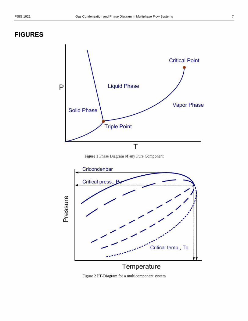
A phase diagram (Figure 1) describes regions of pure

component behavior transitioning between phases. Figure (1)

shows that in pure materials, decreasing the pressure at a fixed

temperature, results in phase change but just at a point (vapor

pressure curve is a line). At extremely high temperatures and

pressures, the liquid and gaseous phases become

indistinguishable. The phase boundary for liquid and gas does

not continue indefinitely, it terminates at a point on the phase

diagram called the critical point. For multi-component systems

phase diagram is more complex and elaborate than that of pure

compounds. Generally, components with widely different

structure and molecular sizes comprise the system. PT

diagram is a graphical representation of phase changes of

compounds that describes the set of pressure-temperature

combinations for the transition zone between the complete

liquid and complete vapor phase. Figure (2) shows an

idealized P-T diagram for a multi component with a fixed

overall composition. There is a region where the two phases

are at equilibrium. The two-phase region that is bounded by

the bubble point and dew point curves is called “phase

envelope”.

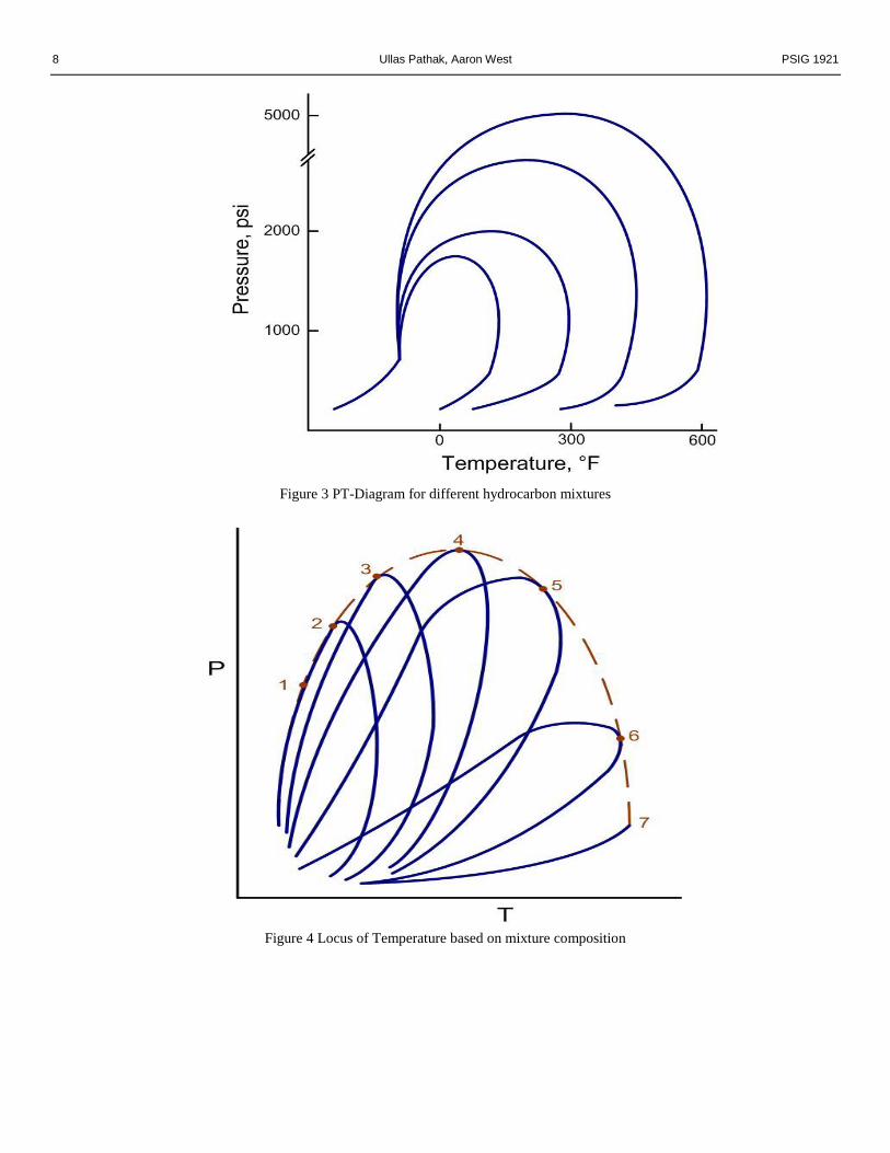
A two-phase mixture has critical temperature which is

between the critical temperatures of the pure components,

presented by the locus of all critical temperature points for

pure components as shown by the dashed line (Figure 4). The

two-phases unlike a pure component can co-exist at a pressure

greater than critical pressure and at a temperature greater than

critical temperature. For a multicomponent system the

maximum pressure that two phases (vapor-liquid) can co-exist

in equilibrium and the maximum temperature that they can

exist in equilibrium, are known as cricondenbar and

cricondentherm, respectively.

The difference between the critical pressure of two component

system and each pure component critical pressure increases by

increasing the difference between the critical points of the two

pure components (Figure 3). A binary mixture cannot exist as

a two-phase system outside the region bounded. To have a

miscibility of two compounds with any composition, at each

temperature the pressure should be higher than the pressure

indicated by the locus of critical pressure line for that specific

temperature. A minimum miscible pressure for each

temperature could be determined according to graph’s data

(Figure 4). Although a lower pressure might be possible for

concentrations when the system will separate into two phases.

When the two-phase mixture enteres the phase envelope and

tends to move towards the liquid phase a timely notification of

these events will help pipeline operators to make effective

decisions. If the different components in the mixture start

condensing and form liquids, it causes hinderance to flow

assurance. The liquid hold-up not only leads to downtime but

also clogging, pressure losses and hence loss in revenue.

These losses can range from 10-15% for gas pipelines.

THERMODYNAMIC MODELING

The thermodynamic behavior of nonideal gas mixtures where

liquid and gas are in equilibrium can be used for the real-time

detection of gas condensation in pipeline monitoring system.

When the gas phase and the liquid phase exist in equilibrium

together, the gas phase fugacity and liquid phase fugacity of

each component is equal.

i.e.

𝑓𝑖𝑔𝑎𝑠

= 𝑓𝑖𝑙𝑖𝑞𝑢𝑖𝑑

(1)

In this work, a gas condensation algorithm (GCA) and

dynamically updated pressure-temperature phase diagram (P-T

diagram) are developed using this principle along with several

other well-known approximations. The Peng-Robinson

Equation of State (PR-EOS), Rachford-Rice Equation, and the

known experimental properties of pure components in the

mixture are all used to model condensation in the pipeline

monitoring system.

The following assumptions have been made in order to

describe the gas-liquid equilibrium:

• The feed compositions are known.

• Each component that condenses is assumed to form a

pure component.

• Quadratic mixing rule for mixtures is used for non-

ideal gas mixtures.

INITIAL PURE COMPONENT PROPERTIES

The acentric factor 𝜔 is a measurement of molecular centricity

of pure components and is used to explain higher boiling

points. Acentric factor (𝜔) can be estimated in various ways.

For reduced boiling temperatures 𝑇𝑏𝑟 =𝑇𝑏

𝑇𝑐 ≤ 0.8 where Tb

denotes the normal boiling temperature and Tc denotes the

critical temperature, the Lee-Kesler methodi was used in this

study.

ω =−ln

Pc1.01325

−5.92714+6.09648

Tbr+1.28862 ln Tbr−0.169347 Tbr

15.2518− 15.6875

Tbr−13.4721 ln Tbr+0.43577 Tbr

(2)

where Pc is in bar.

Otherwise, the Korsten methodii was used in this study.

ω = [0.5899 Tbr

1/3

1 − Tbr1/3

logPc

1.01325] − 1 (3)

where Pc is in bar.

PSIG 1921 Gas Condensation and Phase Diagram in Multiphase Flow Systems 3

PENG ROBINSON EQUATON OF STATE (PR-EOS)

For a pure gas, the PR-EOSiii relates pressure P, molar volume

V, and temperature T as,

𝑃 =𝑅𝑇

𝑉 − 𝑏−

𝑎

𝑉2 + 2𝑉𝑏 − 𝑏2 (4)

where a is given by,

𝑎 = [0.45724𝑅2𝑇𝑐2/𝑃𝑐] [1 + 𝜅 (1 − (

𝑇

𝑇𝑐

)1/2

)]

2

(5)

where 𝜅 is given by,

𝜅 = 0.37464 + 1.54226𝜔 − 0.2699𝜔2 (6)

where, 𝜔 is the acentric factor and b is given by,

𝑏 =0.07780𝑅𝑇𝑐

𝑃𝑐

(7)

For a mixture with N pure components, the PR-EOS can also

be expressed in cubic form as,

Zmix3 − (1 − Bmix)Zmix

2 + (Amix − 2Bmix − 3Bmix2 )Zmix

− ABmix + Bmix2 + Bmix

3 = 0 (8)

where 𝑍𝑚𝑖𝑥 denotes the compressibility of the mixture,

Amix = amix P

R2T2 (9)

Bmix = bmix P

RT (10)

𝑎𝑚𝑖𝑥 = ∑ ∑ 𝑎𝑖𝑗𝑛𝑖𝑛𝑗 (11)𝑁

𝑗=1

𝑁

𝑖=1

𝑎𝑖𝑗 = √𝑎𝑖𝑎𝑗 (1 − 𝑘𝑖𝑗) (12)

𝑏𝑚𝑖𝑥 = ∑ 𝑏𝑖𝑛𝑖 (13)𝑁

𝑖=1

the 𝑘𝑖𝑗 denotes the binary interaction parameter between

components i and j, the ni denotes the mole fraction of the ith

pure component, ai and bi are given for each component i by

equations (12) and (13), respectively.

In this study, the analytical solution (see reference 4 and

reference 5) was used to solve for the compressibility Zmix of

the PR-EOS.

Using the PR-EOS from equation (8), the fugacity coefficient

𝜙𝑖 for the ith component is calculated as,

ln ϕi =(𝑍𝑚𝑖𝑥 − 1)𝑏𝑖

𝑏𝑚𝑖𝑥− ln(𝑍𝑚𝑖𝑥 − 𝐵𝑚𝑖𝑥) −

𝐴𝑚𝑖𝑥

√2𝐵𝑚𝑖𝑥(

1

𝑎𝑚𝑖𝑥

∑ 𝑥𝑖𝑎𝑖𝑗 − 𝑏𝑖

2𝑏𝑚𝑖𝑥

𝑁𝑖=1 ) ln (

𝑍𝑚𝑖𝑥+ (1+ √2)𝐵𝑚𝑖𝑥

𝑍𝑚𝑖𝑥+ (1−√2)𝐵𝑚𝑖𝑥), (14)

where Zmix is the fluid mixture compressibility, 𝐴𝑚𝑖𝑥 =𝑎𝑚𝑖𝑥𝑃

𝑅2𝑇2 ,

and 𝐵𝑚𝑖𝑥 =𝑏𝑚𝑖𝑥𝑃

𝑅𝑇.

GAS CONDENSATION ALGORITHM (GCA)

Using the total mole fractions ni, or compositions, of the N

pure components, the operating temperature T, and the

operating pressure P, GCA ultimately determines the gas mole

fractions yi and liquid mole fractions xi when two phases are

present. The mole fractions are all normalized.

∑ 𝑛𝑖 = 1𝑁

𝑖=1, ∑ 𝑦𝑖 = 1

𝑁

𝑖=1, ∑ 𝑥𝑖

𝑁

𝑖=1= 1 (15)

In turn, the equilibrium constants Ki are defined through the

mixture compressibility Zmix using the operating pressure P,

operating temperature T, gas mole fraction yi, and liquid mole

fraction xi.

𝑙𝑛𝐾𝑖 = 𝑙𝑛𝑦𝑖

𝑥𝑖

= 𝑙𝑛𝜙𝑖

𝑔𝑎𝑠(𝑍𝑚𝑖𝑥 , 𝑦𝑖)

𝜙𝑖𝑙𝑖𝑞𝑢𝑖𝑑(𝑍𝑚𝑖𝑥 , 𝑥𝑖)

, 𝑖 = 1, … , 𝑁 (16)

Using the equilibrium constants Ki and the total mole fractions

ni of the pure components, the total vapor fraction 𝛽 can be

obtained through numerical solution of the Rachford-Rice

equation described in reference 6, and can be expressed as,

𝑔(𝛽) = ∑𝑛𝑖(𝐾𝑖 − 1)

1 + 𝛽(𝐾𝑖 − 1)

𝑁

𝑖=1 (17)

The numerical solution is implemented through a combination

of the bisection method and Newton-Raphson method,

reference 7.

In order to express the Rachford-Rice equation in its form in

equation (17), the gas phase composition yi and liquid phase

composition xi must be related to the equilibrium constants Ki

and total mole fractions ni through the total vapor fraction β by

equations (18) – (20).

𝑦𝑖 =𝐾𝑖𝑛𝑖

1 + 𝛽(𝐾𝑖 − 1), 𝑖 = 1, … , 𝑁 (18)

𝑥𝑖 =𝑛𝑖

1 + 𝛽(𝐾𝑖 − 1), 𝑖 = 1, … , 𝑁 (19)

𝑛𝑖 = 𝛽𝑦𝑖 + (1 − 𝛽)𝑥𝑖 , 𝑖 = 1, … , 𝑁 (20)

4 Ullas Pathak, Aaron West PSIG 1921

If two phases are present, the total vapor fraction β and gas

and liquid mole fractions are solved by an iterative procedure.

In order to initialize the procedure, the approximate Wilson

equilibrium constants Ki are used and are estimated using

generalized correlations, reference 8.

𝑙𝑛𝐾𝑖 = 𝑙𝑛𝑃𝑐,𝑖

𝑃+ 5.373(1 + 𝜔𝑖) (1 −

𝑇𝑐,𝑖

𝑇) (21)

Given the operating pressure P and temperature T, critical

pressure Pc,i, critical temperature Tc,i , and acentric factor 𝜔𝑖 of

the ith component as defined in equation (3), the iterative

procedure, reference 9, is performed as follows:

• The total vapor fraction 𝛽 is determined by solving

the Rachford-Rice equation (17).

• The gas phase mole fractions yi and liquid phase

mole fractions xi are calculated with equations (18)

and (19).

• The fugacity coefficients 𝜙𝑖𝑔𝑎𝑠

and 𝜙𝑖𝑙𝑖𝑞𝑢𝑖𝑑

are

calculated using equations (14) and (16).

• The equilibrium constants Ki are determined from the

fugacity coefficients using equation (21).

The iterations are performed until one of the following

conditions is satisfied.

• The total vapor fraction converges between

successive iterations: |𝛽𝑛 − 𝛽𝑛−1| < 10−7.

• Equilibrium is reached: ∑ (1 −𝜙𝑖

𝑔𝑎𝑠

𝜙𝑖𝑙𝑖𝑞𝑢𝑖𝑑)

2

𝑁𝑖=1 < 10−14

• 𝛽 = 1 or 𝛽 = 0

Now that the total vapor fraction is known, pipeline operators

can set threshold limits of detection for warnings that too

much condensation has occurred in a given pipe.

DYNAMIC PRESSURE-TEMPERATURE PHASE DIAGRAM (PT-DIAGRAM)

Using the properties of the pure components in a mixture, a

dynamic PT-diagram for the mixture is constructed on-the-fly.

First, in order to construct the PT-diagram for the mixture,

vapor-liquid equilibrium (VLE) curves must be constructed

for the pure components. The critical pressures Pc and critical

temperatures Tc are known and stored in advance for each

pure component. Starting at (P c, T c), incrementally decreasing

the temperature, and using the last determined saturation

pressure as an initial guess to the current saturation pressure

Psat, the pure component VLE curves are generated.

Starting at the initial guess Psat, the pressure is lowered until

solving the PR-EOS for the compressibility yields two real

roots: a gas root and a liquid root. Then, by setting N=1, n1=1,

and k11=0, equation (22) reduces to the pure component

version. Then, using the gas and liquid compressibility roots,

the pure component fugacity coefficients 𝜙𝑖(𝑍𝑝𝑢𝑟𝑒𝑔𝑎𝑠

, 1) and

𝜙𝑖(𝑍𝑝𝑢𝑟𝑒𝑙𝑖𝑞𝑢𝑖𝑑

, 1) are determined. At this point, the old saturation

pressure 𝑃𝑠𝑎𝑡𝑜𝑙𝑑 is updated to a new saturation pressure 𝑃𝑠𝑎𝑡

𝑛𝑒𝑤 as

follows.

𝑃𝑠𝑎𝑡𝑛𝑒𝑤 = (𝑃𝑠𝑎𝑡

𝑜𝑙𝑑) (𝑓𝑟𝑎𝑡𝑖𝑜) (22)

where 𝑓𝑟𝑎𝑡𝑖𝑜 is defined as,

𝑖𝑓 |1 −𝜙𝑖

𝑙𝑖𝑞𝑢𝑖𝑑

𝜙𝑖𝑔𝑎𝑠 | < |1 −

𝜙𝑖𝑔𝑎𝑠

𝜙𝑖𝑙𝑖𝑞𝑢𝑖𝑑

| , 𝑓𝑟𝑎𝑡𝑖𝑜 = 𝜙𝑖

𝑙𝑖𝑞𝑢𝑖𝑑

𝜙𝑖𝑔𝑎𝑠 (23)

otherwise,

𝑓𝑟𝑎𝑡𝑖𝑜 = 𝜙𝑖

𝑔𝑎𝑠

𝜙𝑖𝑙𝑖𝑞𝑢𝑖𝑑

(24)

When equilibrium is reached and 𝑓𝑟𝑎𝑡𝑖𝑜=1, the new saturation

pressure 𝑃𝑠𝑎𝑡𝑛𝑒𝑤 converges to the saturation pressure 𝑃𝑠𝑎𝑡 for the

pure component.

It is important to note that as gas flows through the pipeline,

new components might be added into the mixture. When a

new component is added into the mixture, a new pure

component VLE is generated and stored in a permanent

location.

Once all the pure component VLE’s are available for the

current mixture, the mixture PT diagram is constructed and

consists of the connected bubble and dew curves. The

following is performed for each separate pure component.

Starting at the largest critical temperature Tc of all the pure

components, if the temperature T > Tc, a weighted

contribution of the critical pressure Pc based on the mole

fractions is made only to the bubble curve. On the other hand,

if the temperature T <=> Tc, then weighted contributions of

Psat are made to both the bubble curve and the dew curve.

Given the PT diagram for the mixture and the operating

pressure and temperature, pipeline operators can check

dynamically for condensation.

CASE STUDY: PHASE SEPARATION

AND GAS CONDENSATION IN A

PIPELINE

The modeling and simulation have been implemented and

validated at a major oil and gas company’s site on a 1700 km

(~1056 mi) commercial pipeline network being used to

transport ~2700 MMSCFD (million standard cubic foot) of

gas from ~17 reservoir units to different distribution units. The

PSIG 1921 Gas Condensation and Phase Diagram in Multiphase Flow Systems 5

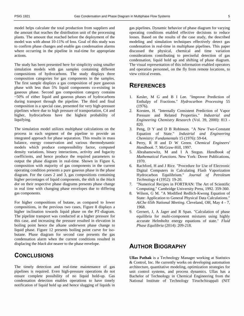
model helps calculate the total production from suppliers and

the amount that reaches the distribution unit of the processing

plants. The amount that reached before the deployment of the

model was with about 10-11% of loss. Goal of this study was

to confirm phase changes and enable gas condensation alarms

where occurring in the pipeline in real-time for appropriate

actions.

The study has been presented here for simplicity using smaller

simulation models with gas samples containing different

compositions of hydrocarbons. The study displays three

composition categories for gas components in the samples.

The first sample displays a gas composition of pure gaseous

phase with less than 5% liquid components co-existing in

gaseous phase. Second gas composition category contains

~50% of either liquid and gaseous phases of hydrocarbons

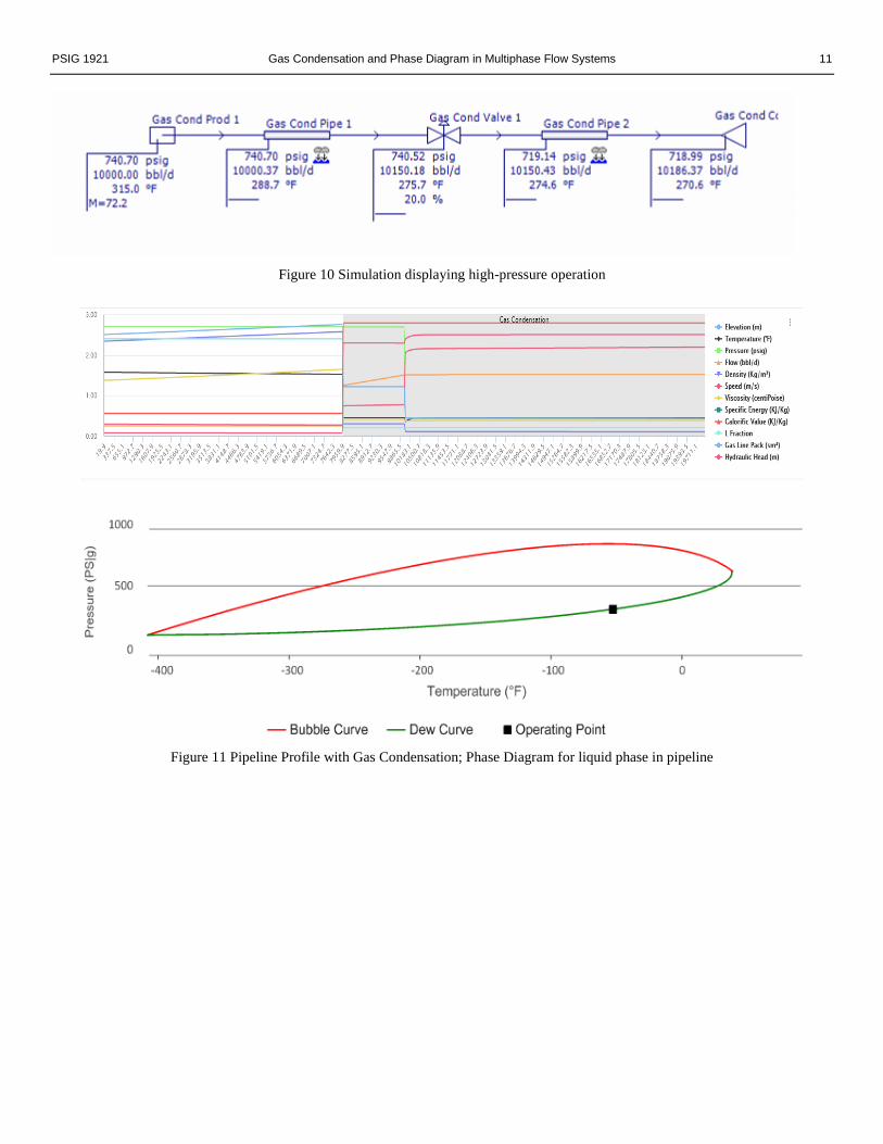
during transport through the pipeline. The third and final

composition is a special case, presented for very high-pressure

pipelines where due to high pressure of transportation, C4 and

higher, hydrocarbons have the highest probability of

liquifying.

The simulation model utilizes multiphase calculations on the

process in each segment of the pipeline to provide an

integrated approach for phase separation. This results in mass

balance, energy conservation and various thermodynamic

models which produce compressibility factor, computed

density variations, binary interactions, activity and fugacity

coefficients, and hence produce the required parameters to

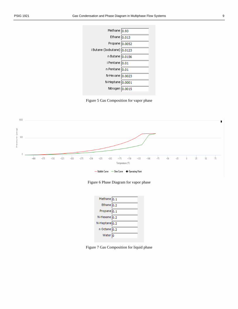
output the phase diagram in real-time. Shown in Figure 6,

composition with majority of gas components in the current

operating condition presents a pure gaseous phase in the phase

diagram. For the cases 2 and 3, gas compositions containing

higher percentages of liquid components, the shift in the black

dot on their respective phase diagrams presents phase change

in real time with changing phase envelopes due to differing

gas components.

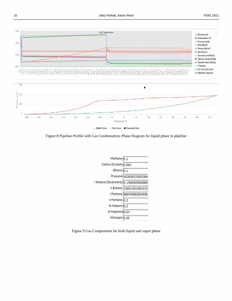
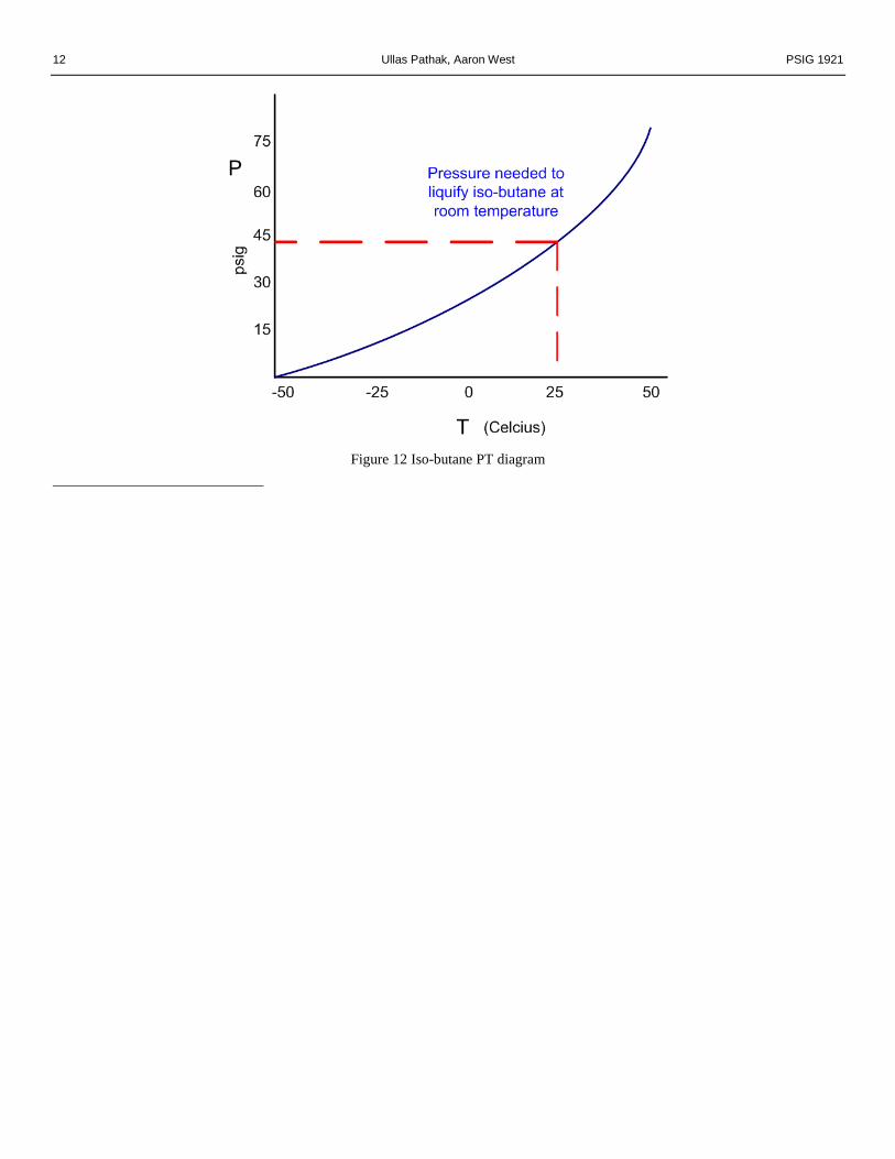
For higher compositions of butane, as compared to lower

compositions, in the previous two cases, Figure 8 displays a

higher inclination towards liquid phase on the PT-diagram.

The pipeline transport was conducted at a higher pressure for

this case, and increasing the pressure resulted in elevation in

boiling point hence the alkane underwent phase change to

liquid phase. Figure 12 presents boiling point curve for iso-

butane. Phase diagram for second case presents the gas

condensation alarm when the current conditions resulted in

displacing the black dot nearer to the phase envelope.

CONCLUSIONS

The timely detection and real-time maintenance of gas

pipelines is required. Even high-pressure operations do not

ensure complete possibility of no liquid hold-up. Gas

condensation detection enables operations to have timely

notification of liquid hold up and hence slugging of liquids in

gas pipelines. Dynamic behavior of phase diagram for varying

operating conditions enabled effective decisions to reduce

losses. Based on the results of the case study, the described

modeling and simulation techniques effectively detect gas

condensation in real-time in multiphase pipelines. This paper

discussed the physical, chemical and time variation

considerations contributing to preciseful detection of gas

condensation, liquid hold up and shifting of phase diagram.

The visual representation of this information enabled operators

and operation personnel, on the fly from remote locations, to

view critical events.

REFERENCES

1. Kesler, M G and B I Lee. "Improve Prediction of

Enthalpy of Fractions." Hydrocarbon Processing 55

(1976).

2. Korsten, H. "Internally Consistent Prediction of Vapor

Pressure and Related Properties." Industrial and

Engineering Chemistry Research (Vol. 39, 2000): 813 -

820.

3. Peng, D Y and D B Robinson. "A New Two-Constant

Equation of State." Industrial and Engineering

Chemistry: Fundamentals 15 (1976): 59-64.

4. Perry, R H and D W Green. Chemical Engineers'

Handbook. 7. McGraw-Hill, 1997.

5. Abrahamowitz, M and I A Stegun. Handbook of

Mathematical Functions. New York: Dover Publications,

1970.

6. Rachford, H and J Rice. "Procedure for Use of Electronic

Digital Computers in Calculating Flash Vaporization

Hydrocarbon Equilibrium." Journal of Petroleum

Technology 4 (1952): 19-20.

7. "Numerical Recipes in FORTRAN: The Art of Scientific

Computing." Cambridge University Press, 1992. 359-360.

8. Wilson, G M. "A Modified Redlich-Kwong Equation of

State: Application to General Physical Data Calculations."

AiChe 65th National Meeting. Cleveland, OH, May 4 - 7,

1968.

9. Gernert, J, A Jager and R Span. "Calculation of phase

equilibria for multi-component mixtures using highly

accurate Helmholtz energy equations of state." Fluid

Phase Equilibria (2014): 209-218.

AUTHOR BIOGRAPHY

Ullas Pathak is a Technology Manager working at Statistics

& Control, Inc. He currently works on developing automation

architecture, quantitative modeling, optimization strategies for

unit control systems, and process dynamics. Ullas has a

Bachelor of Technology in Chemical Engineering from the

National Institute of Technology Tiruchchirappali (NIT

6 Ullas Pathak, Aaron West PSIG 1921

Trichy), a Master of Science in Chemical Analytics from

Arizona State University, and a Master of Engineering in

Biorenewable Technologies from Iowa State University. Ullas

has led many global-energy projects, focusing on optimizing

operations, process enhancement and product engineering.

Dr. Aaron C. West is a Software Engineer working at

Statistics & Control, Inc. He has a Bachelor of Arts in

Chemistry from Augustana College, Bachelor of Arts in

Biology from Augustana College, and Doctor of Philosophy in

Physical Chemistry from the Iowa State University of

Technology. Aaron has over 10 years of experience in the

development and use of computer software for modeling

complex physical processes.

PSIG 1921 Gas Condensation and Phase Diagram in Multiphase Flow Systems 7

FIGURES

Figure 1 Phase Diagram of any Pure Component

Figure 2 PT-Diagram for a multicomponent system

8 Ullas Pathak, Aaron West PSIG 1921

Figure 3 PT-Diagram for different hydrocarbon mixtures

Figure 4 Locus of Temperature based on mixture composition

PSIG 1921 Gas Condensation and Phase Diagram in Multiphase Flow Systems 9

Figure 5 Gas Composition for vapor phase

Figure 6 Phase Diagram for vapor phase

Figure 7 Gas Composition for liquid phase

10 Ullas Pathak, Aaron West PSIG 1921

Figure 8 Pipeline Profile with Gas Condensation; Phase Diagram for liquid phase in pipeline

Figure 9 Gas Composition for both liquid and vapor phase

PSIG 1921 Gas Condensation and Phase Diagram in Multiphase Flow Systems 11

Figure 10 Simulation displaying high-pressure operation

Figure 11 Pipeline Profile with Gas Condensation; Phase Diagram for liquid phase in pipeline

12 Ullas Pathak, Aaron West PSIG 1921

Figure 12 Iso-butane PT diagram