Provided by the author(s) and University College Dublin Library in accordance with publisher

policies. Please cite the published version when available.

Title A new methodology for determining thermal properties and modelling temperature

development in hydrating concrete

Authors(s) O'Donnell, John J.; O'Brien, Eugene J.

Publication date 2003-04

Publication information Construction and Building Materials, 17 (3): 189-202

Publisher Elsevier

Link to online version http://dx.doi.org/10.1016/S0950-0618(02)00099-5

Item record/more information http://hdl.handle.net/10197/2302

Publisher's version (DOI) 10.1016/S0950-0618(02)00099-5

Downloaded 2019-12-31T03:21:16Z

The UCD community has made this article openly available. Please share how this access

benefits you. Your story matters! (@ucd_oa)

Some rights reserved. For more information, please see the item record link above.

1

A New Methodology for Determining Thermal Properties and

Modelling Temperature Development in Hydrating Concrete

John J. O’Donnell BE, PhD, MIEI

Lecturer, Dept. of Civil/Structural Engineering,

Dublin Institute of Technology.

Eugene J. O’Brien MSc, PhD, CEng, FIEI, MIStructE

Head of Civil Engineering, University College Dublin.

2

Abstract

A method is described for determining both the rate of heat generation and the time-dependent thermal properties

of concrete so that the temperature development in a concrete section can be modelled. The method uses measured

temperature data from concrete prisms and involves fitting data from the sample prisms of concrete to a simple

theoretical heat-flow model. It is intended to facilitate on-site tests of concrete mixes; the resulting data can be

used

in computer models to predict the stresses that can lead to early thermal cracking in large pours.

The method is tested by using the thermal properties obtained from the model to predict the temperature versus

time profile at a number of locations in a large rectangular block of concrete and comparing these predictions with

measured temperatures from the block.

3

1. INTRODUCTION

It is well known that the setting of concrete involves exothermic chemical reactions (1). When large concrete

sections, such as thick walls or deep foundations, are being poured it is often required to control (usually

minimise)

temperature rise in the concrete. The simplest control measure that can be adopted is to minimise the rate of

hydration (and consequently the rate of heat generation) in a given member. This can be done by using the

minimum cement content consistent with other design criteria, using a cement with low heat evolution

characteristics

or replacing some of the cement with a pozzolan such as pulverised fuel ash or blast-furnace slag (5). Minimising

the concrete placing temperature and choosing an appropriate formwork type can also be beneficial.

In general, if a large section is being cast the main factor to be controlled is the temperature difference between the

core and the surface. If a thin member cast onto existing mature concrete is involved then the maximum overall

temperature rise is the critical factor.

In order to decide what control method is appropriate and to estimate the thermal stresses that may arise in the

concrete it is of great benefit to be able to estimate the full temperature/time history of the concrete during

hydration. A knowledge is needed of both the rate of heat generation and the other thermal properties of the

concrete if the complete temperature/time history of the concrete structure is to be modelled numerically.

A number of methods have been described in the literature for determining the relevant properties, with most

attention being paid to the rate of heat generation. The use of controlled adiabatic tests has been described by a

number of authors in this context (2,3). In one study, measured temperatures from three adiabatic samples were

combined to determine the heat generation properties of a concrete mix (3). Large insulated blocks have also been

used to approximate adiabatic conditions (4). In another approach isothermal calorimetry on a cement sample was

used to estimate the rate of heat generation (5).

In this paper a method is described whereby three short prisms of fresh concrete are used to estimate the required

thermal properties. While the prisms are stored in different ambient conditions, none have to be stored in a

carefully controlled thermal environment. This flexibility in the thermal environment renders the method

particularly suitable for use on site.

In each prism, temperature is monitored at a number of nodes along the axis. A one-dimensional theoretical model

is then formulated where the unknown properties consist of the thermal properties and the quantities relating to

heat generation. A standard optimisation algorithm is used to find the property values that give the closest match of

theoretical to actual temperature profiles.

4

To test the accuracy of this approach, the property values obtained were used in a finite element model of a large

rectangular block of concrete. The temperature profiles predicted by this model were compared with temperatures

measured in the block. This provided a measure of the accuracy of the thermal property values obtained from the

optimisation.

2. EXPERIMENTAL PROGRAMME

A total of five concrete specimens were cast in the test. They comprised three short prisms, one long prism and one

partially insulated block. The aim was to use measured temperatures from the prisms to predict temperatures in the

block and to compare these predictions with measured values. The long prism was used to determine the heat loss

coefficients for the sides and ends of the prisms.

All specimens were cast indoors using Ordinary Portland Cement. The constituents of the mix are given in Table 1.

Fine aggregate (sand) 545 kg.

Coarse aggregate (10mm) 1010 kg.

Ordinary Portland Cement 595 kg.

Water 230 kg.

Table 1 - Concrete mix constituents, per m3 of concrete

The fine aggregate, coarse aggregate and cement were initially mixed manually as a single batch until a uniform

matrix was obtained. Due to the limited size of the mixer used the addition of the water and the final mixing was

done in two batches, one batch being used for the prisms and the second being used for the block. There was a time

delay of approximately twenty minutes between the mixing of the two batches. This time delay was recorded and

was

allowed for when the results were being analysed.

The short prisms used are illustrated in Figures 1 and 4. All the prisms contained 5mm thick steel plates at the

locations shown. Each concrete prism was 450mm long (including the steel plates) with a 100mm x 100mm cross

section. These plates were placed for purposes outside the scope of this paper. Prism Nos. 1 and 3 were stored at a

room temperature of about 15 oC. Prism No. 2 was initially stored at room temperature and after eight hours was

placed in an oven, at about 50 oC. It was then alternated every eight hours, between the oven environment and the

room temperature environment. This was done so that a temperature difference was always maintained between

the concrete in the prism and its environment.

5

Each prism contained a 20 mm diameter hollow plastic tube along its axis. Thermocouples were placed along the

tube at the locations shown in Fig. 1. The thermocouple wires were passed through the plastic tube to the outside

of each prism. Temperatures were recorded, at fifteen minute intervals, for a period of seven days, the first set of

readings being taken approximately fifteen minutes after the second batch of concrete was mixed. Additional

thermocouples were used to record room and oven ambient temperatures.

The long prism is illustrated in Fig. 2. This prism was 950mm long, including ten 5mm thick metal plates, with a

100 mm x 100 mm cross-section. As for the short prisms it contained a 20mm diameter plastic tube along its axis.

A total of eight thermocouples were placed on the tube at the locations indicated in the figure. The prism was lined

on all sides, except one end face, with 50 mm of dense extruded polystyrene.

The long prism was initially stored in an oven at about 40 oC for a period of two weeks to ensure that the hydration

rate had reduced to a negligible level, that is, the concrete had matured. At the end of the two week period the

prism was initially heated up to a temperature of approximately 50 oC and was then removed from the oven to a

room temperature environment of about 15 OC. Temperatures were monitored along its axis, at five minute

intervals, until it had cooled to within about 5 oC of ambient temperature. The prism was then put back into the

oven (at about 50 oC) and thermocouple readings were again taken at five minute intervals until the prism concrete

had heated up to within 5 oC of oven temperature. This cooling/heating procedure was repeated a number of times

with temperatures being recorded for each cycle. Additional thermocouples were used to record room and oven

ambient temperatures throughout the test.

The block dimensions were 300mm x 500mm x 1000mm as illustrated in Figures 3 and 5. All faces were lined

with 50mm of polystyrene except for one 300mm x 500mm face and one 300mm x 1000mm face which were

lined with plywood only. This arrangement was chosen to simulate a horizontal “slice” through a thick concrete

wall or abutment. Six thermocouples were placed in the block. The gauges were placed in the plane midway

between the two 500mm x 1000mm insulated faces at the locations indicated in the figure. Readings were recorded

at 15 minute intervals for a period of seven days.

Type K thermocouples were used throughout. Each thermocouple was microwelded at its end and connected to a

data-logger. The data-logger was attached to a personal computer which recorded and stored all of the temperature

readings.

3. THEORETICAL DEVELOPMENT

6

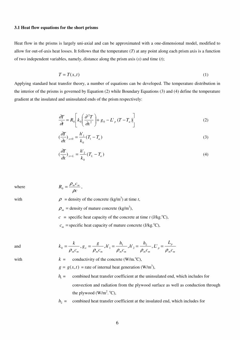
3.1 Heat flow equations for the short prisms

Heat flow in the prisms is largely uni-axial and can be approximated with a one-dimensional model, modified to

allow for out-of-axis heat losses. It follows that the temperature (T) at any point along each prism axis is a function

of two independent variables, namely, distance along the prism axis (x) and time (t);

T T x t= ( , ) (1)

Applying standard heat transfer theory, a number of equations can be developed. The temperature distribution in

the interior of the prisms is governed by Equation (2) while Boundary Equations (3) and (4) define the temperature

gradient at the insulated and uninsulated ends of the prism respectively:

−−+

= )('02

2

00 ap TTLgx

TkR

t

T

∂

∂

∂

∂ (2)

( ) ( )∂

∂

T

x

h

kT Tx a= = −0

1

0

1

' (3)

( )'

( )∂

∂

T

x

h

kT Tx L L a= = −2

0

(4)

where c

cR mm

ρ

ρ=0 ,

with ρ = density of the concrete (kg/m3) at time t,

ρ m = density of mature concrete (kg/m3),

c = specific heat capacity of the concrete at time t (J/kg.oC),

cm = specific heat capacity of mature concrete (J/kg.oC),

and kk

cg

g

ch

h

ch

h

cL

L

cm m

o

m m m m m m

p

p

m m

0 11

22= = = = =

ρ ρ ρ ρ ρ, , ' , ' , '

with k = conductivity of the concrete (W/m.oC),

g g x t= ( , ) = rate of internal heat generation (W/m3),

h1 = combined heat transfer coefficient at the uninsulated end, which includes for

convection and radiation from the plywood surface as well as conduction through

the plywood (W/m2. oC),

h2 = combined heat transfer coefficient at the insulated end, which includes for

7

convection and radiation from the plywood surface as well as conduction through

the insulation and plywood (W/m2. oC),

T1 = temperature on the prism axis just inside the plywood at the uninsulated end ( oC),

Ta = ambient temperature ( oC),

TL = temperature on prism axis just inside the insulation at the insulated end ( oC) ,

Lp = heat loss coefficient for the out-of -axis heat losses (W/m3. oC) .

The normalised total heat generated per unit volume (often called the maturity) at a distance x along the prism axis

up to time t can be expressed as:

Q x t g x t dto

t

t

( , ) ( , )= ∫0

(5)

where Q = normalised total heat generated ( oC), at time t.

The rate of heat generation can be modelled by the Arrhenius equation (6) to give:

+−

+−=

)273(

1

)273(

1exp0

r

rTT

Kgg (6)

where Tr = an arbitrary reference temperature ( oC),

gr = the value of the heat generation parameter at the reference temperature,

and K = E

R is a constant (

oK)

with E = activation energy for the hydration reaction (kJ/mole),

R = Gas Constant (kJ/mole.oK).

273 is added to each oC temperature to convert it to

oK because the Arrhenius equation uses absolute temperatures

in degrees Kelvin.

Substituting Equation (6) in Equation (2) gives:

−−

+−

+−+

= )('

)273(

1

)273(

1exp

2

2

00 ap

r

r TTLTT

Kgx

TkR

t

T

∂

∂

∂

∂ (7)

Equations (3), (4) and (7) determine the temperature distribution in the prisms throughout the hydration period. A

total of seven unknown parameters can be identified in these equations, namely gr, k0, R0,K, h h L p' , ' , '1 2 . The first

two parameters - gr and k0, - representing heat generation and conductivity respectively, are assumed to be unique

8

functions of maturity (Q). The assumption regarding gr is supported by existing literature (10,11). With regard to

k0, the conductivity of concrete does not vary significantly with temperature in the normal ambient range (1) and,

accordingly, it was not considered necessary to allow this parameter to vary as a function of temperature.

Conductivity will change somewhat as the amount of free water in the concrete changes and this in turn depends

on the degree of hydration. Therefore, it is assumed that k0 varies as a function of Q. Both gr and k0, were

determined from the temperature data recorded in the short prisms.

The third parameter c

cR mm

ρ

ρ=0 , can usually be assumed to equal unity as neither the specific heat capacity nor

the density of the concrete vary significantly throughout the main hydration period.

The remaining four parameters - K h h, ,' '1 2 and L’p - are assumed to be constants. This assumption is again

supported by the literature (11). The first of these parameters - K- was determined from the short prisms while the

remaining three were determined from the long prism experiment.

Thus the three parameters representing the heat generation rate and the other thermal properties of concrete,

namely, k0, gr, K, were determined from the short prism data while the three parameters governing the heat loss

rate from the sides and ends of the prism, namely L p' , h'1 and h'2 , were determined from the long prism data. A

computer program was written to find the values for each set of three parameters that give a best fit of measured

temperatures to those predicted by theoretical models of the long and short prisms. The program also calculates Q

at each node along the prism at the end of each time step. The program solves the heat flow equations, given

above, using the finite difference method and uses a standard, least squares, optimisation procedure to find the

best-fit values for the unknown parameters.

3.2 Heat Flow Equations for the Long Prism

As the concrete is mature in the long prism when the temperature measurements are being taken, hydration will

have dropped to negligible levels. Therefore, the heat generation term can be set to zero and the R term will equal

unity. The temperature/ time gradient for any point along the axis of the prism can be expressed as:

∂

∂

∂

∂

T

tk

T

xL T Tm p a= − −

0

2

2( ) ' ( ) (11)

where k m0( ) = value of the conductivity parameter 0k for mature concrete

9

Since the long prism cross section is the same as that used for the short prism, the loss factor L’p will also be the

same. The boundary equations are the same as those already given in Equations (2) and (3) for the short prism.

The loss term, L p' , was found as follows. Consider the plane of cross-section A-A through the long prism located

halfway along the prism axis (Fig. 2). When there is a temperature difference between the prism concrete and the

surrounding air, heat flow will occur in this plane. The results of a number of numerical tests, using the finite

difference program, showed that, for a prism of this length, the heat flow along the axis of the prism at the location

A-A is insignificant compared with the out-of-axis heat flow in the plane of the cross-section. Therefore, the

temperature time gradient at the centre of cross-section A-A can be expressed as:

∂

∂

T

tL T Tc

p c a= −' ( ) (12)

where Tc = temperature at the intersection of the prism axis and section A-A

L p' = loss factor for prism cross-section

In the laboratory the ambient temperature is relatively constant in comparison with the prism temperature which is

changing quite rapidly. Therefore Equation (12) can be rewritten as:

∂

∂

∂

∂

T

t

T

tL Tc d

p d≈ = ' ( ) (13)

where T T Td c a= −( ) is the difference in temperature between the prism axis, at

location A-A, and ambient temperature.

The solution to this differential equation is

T L t Cd p= +exp( ' ) (14)

where C = an unknown constant.

Taking the natural log of both sides we get

ln ln ' ( ' ' )T C L t C L td p p= + = + (15)

where C’ = lnC = a constant

10

If the long prism is heated up in an oven and is then allowed to cool in a room temperature environment then

Equation (15) can be applied to the cooling phase. By plotting ln Td against t over a period of time and fitting a

straight line to the data, an estimate of L’p is obtained. Similarly Equation (15) can be applied when the prism is

being heated up from ambient to oven temperature with L’p , in this case, being a heat gain factor.

3.3 Variation of Thermal Properties during Hydration

Two of the unknown parameters determined from the short prism analysis, gr and k0, are assumed to be functions of

Q. In order to model these parameters using the computer program described at the end of Section 3.1, some

assumptions had to be made about how these parameters vary over the range of Q. Two different methods were

initially considered; a Global and a Local method. In both approaches the two parameters were assumed to be

either constants throughout the time interval or specified functions of Q. A combination of the Local and Global

methods was finally adopted when determining the best-fit values for the unknown parameters.

In the Local analysis method the Q range is divided up into a number of ‘maturity’ bands. Within each band the

heat generation term - gr - is assumed to vary linearly with Q. Thus:

g Q g g Qr ( ) = +1 2 for each band (16)

where g g1 2, are constants

The k0, term is assumed to be constant within each band. Thus, for each maturity band, the short prism analysis

was reduced to finding values for four constant parameters - g1, g2, k0, and K, The values of these four parameters

are allowed to vary from one maturity band to the next so that the properties have freedom to vary across the Q

range. An optimisation is done for each band to find the values of the parameters that give a best fit of measured

temperatures to those calculated by the theoretical model.

The Local Method of analysis has a number of complications. Firstly, for a given prism at any given time, the

nodes along the prism axis will be hydrating at different rates and will therefore have different values of Q at any

particular time. This can be illustrated by means of an example. Fig. 6 shows a typical case of a prism where

temperatures are being monitored at four nodes along the prism axis.

Temperature readings are taken at each node at times t0, t1, t2 and t3. Q(i,tj ) and T(i,tj ) represent the values of Q

and T at node i, at time tj. In the figure the value of Q is plotted on the vertical axis for each node at the end of each

time step (it should be noted that in a real example the Q values at the end of each time step will not be known in

advance). The Q range is divided into three maturity bands in this case. These bands are indicated, in the diagram,

by the dotted lines.

11

The figure illustrates how, at any given time (t), the different nodes will have different values of Q. For example,

at time t1 the Q value for node 1 lies in Band 2 while the Q values for nodes 2, 3 and 4 lie in Band 1. It is clear,

therefore, that before optimising to find the unknown parameters for any band the temperature readings whose Q

values fall into that band must be identified. In the example illustrated in Fig. 6 only four temperature readings

have Q values that fall into Band 1, namely, T(2,t1), T(3,t1), T(4,t1) and T(4,t2). Therefore only these four readings

should be used in the optimisation for Band 1.

An iterative method has been developed to identify the temperature readings relevant to each Q band. The method

is started by analysing all of the temperature readings (sixteen in the example illustrated in Fig. 5) to get an initial

estimate of parameter values for Band 1. These parameter values are then used to calculate Q values corresponding

to each temperature reading and any readings with Q values outside Band 1 are eliminated. A second run is carried

out with the remaining set of temperature readings to get an improved estimate of the parameter values for Band 1

and these are again used to calculate Q values for each reading. Again any readings with Q values outside Band 1

are eliminated and the optimisation is repeated with the new data set. This procedure is repeated in an iterative

manner until the temperature readings relevant to Band 1 have been identified and the corresponding best-fit

parameter values have been obtained.. A similar analysis is then carried out for Band 2, Band 3 etc.

It is clear that this iterative procedure requires a large number of optimisations to identify the temperature readings

relevant to each band. This makes the Local optimisation method computationally slow. The second difficulty that

arises with the Local Method is that discontinuities tend to occur between adjacent bands for the optimised values

obtained for the various parameters. This occurs because each band is treated as a separate optimisation problem

without regard to continuity with adjacent bands.

Because of the complications arising from the Local Method an alternative approach was examined. This second

method was designated “the Global Method”. In the simplest version of the Global Method a single equation is

used to represent each unknown property for the entire range of Q. Therefore all of the temperature data is

analysed in a single run. This method eliminates both the banding and discontinuity problems discussed in the

previous section. It is also much faster, computationally, than the Local Method. However, the major difficulty

with the method is finding a single equation that accurately reflects the variation of each property as a function of

Q. In general, for the Global Method, the parameters K, h'1 and h'2 are assumed to be constants, k0 is assumed to

vary linearly with Q and gr is assumed to be given by an exponential type function of Q. In practice, it was found

that gr cannot be accurately represented by a single equation. Typically two or more equations are required, each

applying to a different part of the Q range, to give a good match to measured data. However this does not alter the

principle that one set of equations is used for each parameter to describe its variation over the full range of Q.

After a trial and error process involving the comparison of Local and Global results obtained from the short prism

data it was found that the g0 parameter could be represented adequately by the following functions:

12

( ) [ ]3

32

2

31 )(exp)()( gQggQgQg r +−+= for Q < 30 (17)

= C1(-C2Q1.5

) for Q > 30 (18)

where g1, g2, g3, C1 and C2 are constants

The constants C1 and C2 were chosen to ensure continuity of both the function value and its first derivative about

the point Q = 30. Thus C1 and C2 were determined by the values of g1, g2 and g3 and were not additional variables.

The short prism analysis, therefore, involved finding the values for five constant parameters - g1, g2, g3, K and k0 -

that give a best fit of measured temperature in the three short prisms to those predicted by a theoretical model.

3.4 Heat Flow Equations for the Large Block

The temperature at an internal point in the mid-plane of the block (midway between the two 500mm X 1000mm

faces) is given by the two-dimensional version of Equation (2) with R0 again being taken to equal unity. As for the

prism, the out-of-plane losses at any point are proportional to ( T Ta− ) where T , in this case, is the temperature at

the relevant point on the mid-plane. Therefore, the temperature-time gradient, at an internal point on the mid-plane

of the block, is given by:

−−++= )()( 02

2

2

2

0 ab TTLgy

T

x

Tk

t

T

∂

∂

∂

∂

∂

∂ (19)

where Lb = heat loss factor to allow for losses perpendicular to the mid-plane of the block

The boundary equations for the four side-wall boundaries are all of the form

)('

)(0

aSS TTk

h

s

T−=

∂

∂ (20)

where 'h = combined convection and radiation coefficient for the boundary.

Ts = temperature of the concrete just inside the insulation or plywood

=Ss

T)(

∂

∂ temperature gradient at the surface where the s direction is normal to surface

The other terms are as previously defined.

3.5 Finite Element Model for the Large Block

13

The heat-flow in the large block was modelled using a two-dimensional finite element heat-flow model

representing

the mid-plane of the block (see Fig. 3 - Sectional Plan). A heat loss factor was included to account for out-of-plane

heat losses. In reality, as the block is 3-dimensional, the method adopted introduces a level of approximation and

there may be some 3-D effects that are not allowed for in the model used. An eight-node rectangular element was

chosen for the model.

The rectangular block was modelled with an 8 x 4 grid of these elements with each element being 0.125 metres

square. The time-step used in the analysis was 150 seconds.

Additional computer code was developed by the first author to allow for a time-varying rate of heat generation,

(specifically a rate of heat generation that varied as a function of the total heat generated to date) as well as

convection and radiation heat loss from the surface of the block

4. RESULTS

4.1 Long Prism Analysis

The first part of the long prism analysis involved estimating the heat loss factor, L’p, which governs the out-of-axis

heat loss/heat gain. The out-of-axis heat flow at the midpoint along the prism axis is governed by Equation (15).

The long prism was initially placed in an oven, at a temperature of approximately 50 oC, for a period of two weeks.

It was then removed from the oven and temperatures were recorded along its axis as it cooled from 50 oC towards

an ambient room temperature of about 20 oC. Fig. 7 illustrates a plot of ln(Td) versus t for this data. The

temperature difference, Td was obtained by subtracting the ambient temperature recorded outside the prism from

the temperatures recorded by the temperature gauge located at the centre point of the prism axis (Gauge No. 5). It

can be seen that the plot of ln(Td) versus t is virtually linear.

The second part of the long prism test involved monitoring temperatures in the prism as it was being heated up

from a temperature of about 25 oC towards an oven temperature of 50

oC. When ln(Td) is plotted against t for this

case a similar plot to that in Fig. 7 is obtained. The whole heating and cooling procedure was then repeated a

number of times resulting in a number of plots similar to those in Fig 7. For each such plot, linear regression was

used to find the best-fit straight line through the data points and the slope of each such line was calculated. It is

clear from equation (15) that the slope of these lines is a measure of L’p.

14

From a comparison of the slopes the heat loss factor and the heat gain factor were found to be approximately

equal. Accordingly, the average of all the slopes was obtained and this figure was adopted as an estimate for the

heat loss/heat gain factor Lp’. The following value was obtained from this analysis:

L’p = 1.09 × 10

-5 sec

-1.

This value was adopted in subsequent analyses for both the long and the short prisms.

The second part of the long prism test involved an analysis of heat flow along the prism axis. The temperature/time

gradient at any point along the axis of the long prism is given by Equation (11). The boundary equation for the two

ends are given by Equations (3) and (4). Equations (3), (4) and (11) together contain three unknown parameters,

namely, ko(m), h’1 and h’2. The optimisation procedure was used to find the values of these three parameters that

gave a best-fit of measured temperatures, along the long prism axis, to those predicted by a theoretical model. The

optimised parameter values obtained from this analysis were as follows:

ko(m) = 8.27 × 10-7

m2/sec

h’1 = 1.40 × 10

-6 m/sec

h’2 = 1.68 × 10-7

m/sec

A typical temperature versus time profile obtained from these parameter values is illustrated in Fig. 8 for Node 1 in

the long prism when the prism is losing heat. Figs. 9(a) and 9(b) illustrate actual and best-fit theoretical

temperature profiles along the prism axis for one particular time for both the “losing heat” and “gaining heat”

phases. It can be seen that a reasonably good match has been obtained between actual and best-fit theoretical

temperatures.

4.2 Short Prism Analysis

The measured temperature data from the short prisms was analysed to find the unknown parameters relating to

heat generation and conductivity. The temperature/time gradient, along the axes of the short prisms, is given by

Equation (2). The boundary conditions at the insulated and uninsulated ends of the prisms are defined by

Equations (3) and (4). These three equations contain six unknown parameters - k0, gr, K, L’p, h’1 , and h’2. The

15

three latter parameters were determined from the long prism analysis as described in Section 4.1. Thus, only three

parameters - k0, gr and K - remained to be determined from the short prism data. These are the parameters which

define the concrete conductivity, the rate of heat generation and the temperature dependence of the rate of heat

generation respectively.

The long prism analysis determined the parameter k0(m) which represents the conductivity of mature concrete. The

general conductivity parameter, k0, was assumed to vary linearly as a function of Q, reaching a value of k0(m) at Q =

Qmax where Qmax is the maximum Q value obtained at the end of the period during which temperature data was

recorded. Thus the conductivity parameter was assumed to be given by:

k0(Q) = k0(m) +k1(Qmax - Q) (19)

where k1 = an unknown constant

The heat generation parameter gr was assumed to be given by Equations (17) and (18). Thus the short prism

analysis was reduced to finding the values of five constant parameters - g1, g2, g3, K and k1. The best fit results

were as follows:

g1 = 4.38 × 10-6

g2 = 6.26 × 10-5

g3 = 11.56

K = 6019 (oK)

k1 = 1.94 × 10-8

Actual and best-fit theoretical temperature versus time profiles resulting from these best-fit values, for one

representative node in each prism, are illustrated in Fig. 10. There is quite good agreement between measured and

predicted profiles indicating that the theoretical model has modelled, reasonably accurately, the generation and

flow of heat in the short prism samples. Accordingly, the best-fit values given above were used to make the

temperature predictions in the block.

4.3 Temperature Predictions for Block

The block is illustrated in Fig. 3. A finite element analysis of this block was carried out using the best-fit thermal

property parameters given in Sections 4.1 and 4.2. The optimised h1‘ and h2

‘ parameters were used as heat loss

coefficients for the insulated and uninsulated sides of the block respectively. It should be noted that the heat loss

16

coefficients h1‘ and h2’ are not strictly applicable to the boundaries of the block. These loss coefficients were

obtained for the ends of the prisms and could include some corner or end effects which are specific to the prism

and therefore not strictly applicable to the block. Also there may be corner effects in the block which are not

allowed for in the finite element model. However, it was felt that these coefficients were sufficiently accurate for

the purposes of the model. Fig. 11 illustrates measured and predicted temperature versus time profiles for Gauge

Nos. 1, 2, 3, 5 and 6 in the block. Node 4 has been omitted as its plot is very similar to Node 1.

In general, there is reasonable agreement between measured temperatures and those predicted by the theoretical

model. While the shapes of the actual and theoretical temperature profiles are somewhat different, in general the

discrepancies are relatively small. All of the graphs show a noticeable deviation between predicted and measured

temperatures between approximately fifteen hours and twenty-five hours after the pour with the theoretical profiles

showing a sharper peak than the measured profiles. However, the predicted and measured peak temperatures are

within 2.5 oC of each other at all of the nodes. Only one thermocouple showed a persistent deviation between

predicted and measured temperatures. This occurred at node 3, which gave a predicted temperature consistently

lower than the measured temperature after the peak had been reached. This could possibly be explained by the fact

that the optimised heat loss coefficients h1‘ and h2’ do not adequately model the corner of the block.

On site, for most practical situations, the temperature profile at the centre and near the surface of a section will be

the most critical. The results of the above test give reasonably good agreement between predicted and measured

temperature for the centre (node 5) and the midside surface (node 6) of the block.

5. CONCLUDING COMMENTS

A method for determining the thermal properties of concrete is described. It is shown that the method produces

properties that can be used to predict, with reasonably good accuracy, the temperature/time profile at various

locations in a large concrete member. It is also illustrated how the method can be used to predict the degree of

hydration at any point in a concrete specimen.

Various methods have been described in the literature for determining both the rate of heat generation and the

temperature rise in concrete due to hydration (2, 3, 4, 5). However, the method described in this paper (hereafter

called the prism method) does have some new features that make it particularly suitable for use on site:

(i) The prism samples do not have to be stored in a strictly controlled thermal environment.

(ii) Continuous predicted temperature/time profiles can be obtained from the finite element model. Most currently

used temperature prediction methods only predict peak temperature and/or the maximum temperature difference

within the structure.

(iii) The finite element model can be used to assess the affect on temperature of various activities on site. For

example, if the contractor wants to remove his shuttering from a particular member after, say, two days the finite

17

element model could be used to assess the effect that this would have on the maximum temperature difference

occuring in that member.

(iv) The prism method of calculating the total heat generated (Q), is based on temperature measurements from

prisms made with the same concrete as that used in the main structure. In contrast, the maturity and degree of

hydration methods of strength prediction currently in use involve general functions which can be applied to any

given mix. Thus the prism method should be more reliable if a non-standard mix was used.

(v) The prism method can also predict the total heat generated (Q) in the concrete at any given location and time

and this can be used to predict the strength of the concrete. Therefore, temperature and strength predictions can be

obtained using a single method whereas, at present, separate methods are required.

The prism method has a number of potential practical applications. Firstly it could be used on site throughout the

construction phase of a project to make temperature and strength predictions for the various concrete pours. Ideally

a set of prisms would be cast each time there is a (large) concrete pour. In this way, a database of information

would be built up, which would provide information for ongoing temperature and strength predictions that would

be useful in controlling operations on site. For example, the temperature and strength predictions could be used to

decide the timing of operations such as formwork removal and the application of post-tensioning forces.

Secondly the prism method could be used as part of a trial mix process. For example, if a certain concrete mix was

being proposed for a large concrete structure there might be concerns that large temperature rises could occur,

which could lead to lead to early thermal cracking. In this situation it would be possible to do a trial mix, cast and

monitor some prisms and, using the measured temperatures from the prisms, make temperature predictions for the

main structure. If the predicted temperatures were too high the concrete mix could be adjusted or some other

method specified to limit temperature rise.

18

1 2 3 4 5 6 7 8 9

10 41 63 45 56 53 52 48 39

1 2 3 4 5 6 7 8 9

11 43 53 52 55 51 52 42 45

1 2 3 4

48 103 38

12

20mm Plywood

50mm Insulation

5mm Steel Plate

Thermocouples

attached to plastic

tube

Concrete

Prism Number 1

Prism Number 2

Prism Number 3

Cross-section

20mm dia. plastic tube

450

450

450

100

100

Fig. 1 Short Prism Details

19

1 3 4 5 6 7 8

12

57 317 105 273 75

20mm Plywood

50mm Insulation

5mm Steel Plate

Thermocouples

attached to

plastic tube

Concrete2

42

950

A

A

47

Fig. 2 Long Prism Details

1 2

3 4

5

6

50m m Insulation

C oncrete

Sectional E levation

300

20m m P lywood

500

1000

Sectional P lan

Therm ocouples

Fig. 3 Block Details

20

Fig. 4 Prism Number 2 (prior to pour)

Fig. 5 Block with temperature gauges (prior to pour)

21

Q

Q(1,t3)

Q(2,t3) BAND 3

Q(1,t2)

Q(3,t3)

Q(2,t2)

BAND 2

Q(1,t1) Q(3,t2) Q(4,t3)

Q(2,t1) Q(4,t2)

Q(3,t1)

Q(4,t1) BAND 1

Q(1,t0) Q(2,t0) Q(3,t0) Q(4,t0)

1 2 3 4 Node Number

Fig. 6 Example of maturity bands for nodes along prism

22

2.5

2.6

2.7

2.8

2.9

3

3.1

3.2

3.3

3.4

0 36000 72000 108000 144000 180000

Time (hours)

ln(T

d)

20 30 40 5010

Fig. 7 Plot of log of Td versus time for centre of long prism when losing heat

23

25

27

29

31

33

35

37

39

41

43

0 18000 36000 54000 72000Time (hours)

Te

mp

. (

oC

)

node 1 - meas.

node 1 - theory

15 205 10

Fig. 8 Temperature versus time profile at Node 1 for long prism losing heat

23

Note: In all subsequent figures measured temperatures are shown as individual black squares and

calculated temperatures as a solid line.

20

21

22

23

24

25

26

27

00.20.40.60.81

Distance from exposed surface (m)

Te

mp

. (

oC

)

0.2 0.4 0.6 0.8 1.0

(a) Prism losing heat

Fig. 9 Temperature profile along the long prism axis at 22.75 hours

38

39

40

41

42

43

44

45

46

00.20.40.60.81

Distance from exposed surface (m)

Te

mp

. (

oC

)

0.2 0.4 0.6 0.8 1.0

(b) Prism gaining heat

Fig. 9 Temperature profile along the long prism axis at 22.75 hours

24

15

20

25

30

35

40

0 10 20 30 40 50 60 70 80

Time (hours)

Te

mp

. (

oC

)

(a) Prism No. 1, Node 3

Fig. 10 Temperature Profiles in Short Prisms

15

20

25

30

35

40

0 10 20 30 40 50 60 70 80

Time (hours)

Te

mp

. (

oC

)

(b) Prism No. 3, Node 3

Fig. 10 Temperature Profiles in Short Prisms

25

0

10

20

30

40

50

60

0 10 20 30 40 50 60 70 80Time (hours)

Te

mp

(oC

)Prism moved from

room to oven

Prism moved from

oven to room

(c) Prism No. 2, Node 3

Fig. 10 Temperature Profiles in Short Prisms

10

15

20

25

30

35

40

45

50

55

0 10 20 30 40 50 60 70 80

Time (hours)

Te

mp

. (

oC

)

(a) Node 1

Fig. 11 Temperature versus time profiles in the Block

26

10

15

20

25

30

35

40

45

50

55

0 10 20 30 40 50 60 70 80

Time (hours)

Te

mp

. (

oC

)

(b) Node 2

Fig. 11 Temperature versus time profiles in the Block

10

15

20

25

30

35

40

45

50

55

0 10 20 30 40 50 60 70 80

Time (hours)

Te

mp

. (

oC

)

(c) Node 3

Fig. 11 Temperature versus time profiles in the Block

27

10

15

20

25

30

35

40

45

50

55

0 10 20 30 40 50 60 70 80

Time (hours)

Te

mp

. (

oC

)

(d) Node 5

Fig. 11 Temperature versus time profiles in the Block

10

15

20

25

30

35

40

45

50

55

0 10 20 30 40 50 60 70 80

Time (hours)

Te

mp

. (

oC

)

(e) Node 6

Fig. 11 Temperature versus time profiles in the Block

28

REFERENCES

1. Neville, A.M., (1995) Properties of concrete (4th Edition), Longman.

2. De Sitter, W.R. and Ramler J.P.G., (1991) "The Concrete Hardening Control System: CHCS" in Testing during

Concrete Construction, Proc. of an Int. RILEM Workshop, ed. H.W. Reinhardt, Chapman & Hall, pp

224-243.

3. Harada, S., Suzuki, Y. and Maekawa, K., (1990) "Coupling analysis of heat generation and diffusion for massive

concrete" in Computer Aided Analysis and Design of Concrete Structures, Proceedings of SCI-C,

Second International Conference, ed. N. Bicanic, and H. Mang, Zel am See, Austria, pp.785-797.

4. Trinhztfy, H. W., Blauwendraad, J. and Jongendijk, J., (1981) "Temperature development in concrete structures

taking account of state dependent properties", International Conference on Concrete at Early Ages,

RILEM, pp 211-218.

5. Harrison, T. A., (1978) "Early age temperature rises in Concrete Sections with reference to B.S.5337:1976",

Interim Technical Note No. 5, Cement & Concrete Association.

6. O'Brien, E.J., O'Donnell, J.J., Waldron, P. and El-H.Lahlouh., (1992) "Non-linear Conduction Modelling of

Concrete Walls under the Influence of Heat of Hydration of Cement" in Advanced Computational

Methods in Heat Transfer II ,Vol. 1:Conduction,Radiation and Phase Change, eds. R.C. Wrobel,

C.A. Brebbia, A.J. Novak, Computational Mechanics Publications & Elsevier Applied

Science,Milan, pp 121-130.

7. O'Donnell, J.J., O'Brien, E.J., Waldron, P. and El-H. Lahlouh., (1993) "Prediction of Early Age Strength in

Concrete" in Concrete 2000, Economic and durable construction through excellence, Vol. 1:

Design,Materials,Construction, eds. R.K. Dhir and M.R. Jones,E & FN Spon,Dundee, pp 839-845.

8. Rao, S.S., (1984) Optimisation Theory and Applications, John Wiley & Sons.

9. O'Brien, E.J. and O'Donnell, J.J., (1993) "The Effectiveness of Optimization Techniques for Material Property

Characterization", in Computational Methods and Experimental Measurements, Vol. 2: Stress

Analysis, eds. C.A. Brebbia and G.M. Carlomango, Computational Mechanics Publications &

Elsevier Applied Science,Siena, pp 45-56.

10. Thurston, S. J., Priestley, M.J.N. and Cooke N., (1980) "Thermal Analysis of Thick Concrete Sections", Journal

of the American Concrete Institute, 77, 5, Sept-Oct. 1980, pp 347-357.

11. Wang, C. and Dilger, W.H. (1995) “Prediction of Temperature Distribution in Hardening Concrete” in Thermal

Cracking in Concrete at Early Ages, Proc. of the Int. RILEM Symposium, ed. R Springenschmid, E &

FN Spon, pp 21-28.