proton acceleration through a charged cavity created by
TRANSCRIPT

Proton acceleration through a charged cavity created by ultraintenselaser pulse
Ter-Avetisyan, S., Singh, P. K., Cho, M. H., Andreev, A., Kakolee, K. F., Ahmed, H., Scullion, C., Sharif, S.,Hadjisolomou, P., & Borghesi, M. (2019). Proton acceleration through a charged cavity created by ultraintenselaser pulse. Physics of Plasmas, 26(10), [103106]. https://doi.org/10.1063/1.5100094
Published in:Physics of Plasmas
Document Version:Peer reviewed version
Queen's University Belfast - Research Portal:Link to publication record in Queen's University Belfast Research Portal
Publisher rightsCopyright 2019 AIP. This work is made available online in accordance with the publisher’s policies. Please refer to any applicable terms ofuse of the publisher.
General rightsCopyright for the publications made accessible via the Queen's University Belfast Research Portal is retained by the author(s) and / or othercopyright owners and it is a condition of accessing these publications that users recognise and abide by the legal requirements associatedwith these rights.
Take down policyThe Research Portal is Queen's institutional repository that provides access to Queen's research output. Every effort has been made toensure that content in the Research Portal does not infringe any person's rights, or applicable UK laws. If you discover content in theResearch Portal that you believe breaches copyright or violates any law, please contact [email protected].
Download date:12. Dec. 2021

1
Proton acceleration through a charged cavity created by ultraintense laser pulse
S. Ter-Avetisyan1, , P. K. Singh2, M. H. Cho2, A. Andreev1, K. F. Kakolee2, H. Ahmed3, C. Scullion3, S.
Sharif4, P. Hadjisolomou3, and M. Borghesi3
1ELI-ALPS, Szeged 6728, Hungary
2Center for Relativistic Laser Science, Institute of Basic Science, Gwangju 61005, South Korea
3School of Mathematics and Physics, The Queen’s University of Belfast, Belfast BT7 1NN, UK
4Department of Physics and Photon Science, Gwangju Institute for Science and Technology, Gwangju
61005, South Korea
The potential of laser-driven ion beam applications is limited by high quality requirements. The excellent
“point-source” characteristics of laser accelerated proton beam in a broad energy range was found by using proton
radiographs of a mesh. The “virtual source” of protons, the point where the proton trajectories are converging and
form a waist, gradually decreases and moves asymptotically to the target with increasing particles’ energy.
Computer simulations confirmed that the beams profile at the centre is fully conserved, the “virtual source” of
higher energy protons gradually moves closer to the target, and if the particles energy is further increased the
“virtual source” will be located on the target front surface (for portions above 13 MeV, in this case) with a size
comparable to the laser spot size. The laser ponderomotive force pushes the electrons deep into the target creating
a bipolar charge structure, i.e., an electron cavity and spike which produces strong accelerating field, realising a
point-size source of accelerated protons. This behaviour has had not previously been predicted. These results
contribute to the development of next generation laser-accelerators suitable for many applications.
Thi
s is
the
auth
or’s
pee
r re
view
ed, a
ccep
ted
man
uscr
ipt.
How
ever
, the
onl
ine
vers
ion
of r
ecor
d w
ill b
e di
ffere
nt fr
om th
is v
ersi
on o
nce
it ha
s be
en c
opye
dite
d an
d ty
pese
t.
PL
EA
SE
CIT
E T
HIS
AR
TIC
LE
AS
DO
I: 1
0.1
063/1
.5100094

2
Introduction
Recent advances in laser technology have led to an extremely intense and high contrast laser pulses which have
made realistic to develop laser-driven ion sources as a reliable, generic technology for applications [1-3].
Laser-driven protons have already opened up new research areas e.g. proton probing or proton radiography [4,5]
by studying the transient plasma fields with unprecedented temporal and spatial resolution, despite the current
technology not meeting the required ion beam parameters for many applications. Proton source and beam
characteristics are dominated by the ion acceleration scheme and laser pulse parameters.
Ions are created and accelerated in a quasi-static electric field arising from the displacement of hot electrons
created by the laser field along the target normal. These ions have maximum energy in the forward direction, the
laser propagation direction. In general, charge displacement can occur at the place of laser pulse interaction with
the target where electrons, driven mainly by the laser ponderomotive force, electrostatically couple their energy
to the ions [6,7,8], or, the ions are accelerated through a self-consistent electrostatic field generated by fast
electrons escaping in vacuum at the target rear [9] – the target-normal-sheath-acceleration (TNSA).
These processes are not mutual expulsive and the dominance of one mechanism depends on the interaction
conditions – the target and laser parameters [10]. However, at oblique laser incidence on µm thick target, the
rear side acceleration, i.e. TNSA is the dominant process because inherent laser pre-pulse or pedestal create a
preplasma at the front of the target and, therefore, only at the rear of the target is it possible to maintain the high
gradient of electron temperature and density, and hence, high accelerating field. Ejection of hot electrons to the
backside of the target include phenomena such as the fountain effect [11], electron recirculation through the foil
[12,13] and electromagnetic surface field excitation and propagation [14] which lead to the transverse expansion
of the hot electrons along the target surface. Consequently, ion acceleration takes place at the target rear from
much larger area than laser focal spot, from about 100s of micrometres area [15] typically with 40 - 60 cone
angles [16], known from TNSA scenario [17]. Because the emission of those protons is laminar the concept of
“virtual source” was implemented to describe the proton source/beam properties [4, 5]. Assuming the straight line
trajectories of protons, the “virtual source” is the point from where the protons “straight line trajectories” virtually
originate. In TNSA scenario it was found that the “virtual source” size is in the order of 10s micrometres and
located 100s of micrometres in front of the target [18].
This paper examines laser driven proton source and beam characteristics at intensity of 1020 W/cm2 with
pulse length 30 fs using mesh proton radiography. Measurements show that having very high contrast laser pulse
(the ratio of peak intensity to pre-pulse or pedestal intensity) results in the protons, in a broad energy range,
Thi
s is
the
auth
or’s
pee
r re
view
ed, a
ccep
ted
man
uscr
ipt.
How
ever
, the
onl
ine
vers
ion
of r
ecor
d w
ill b
e di
ffere
nt fr
om th
is v
ersi
on o
nce
it ha
s be
en c
opye
dite
d an
d ty
pese
t.
PL
EA
SE
CIT
E T
HIS
AR
TIC
LE
AS
DO
I: 1
0.1
063/1
.5100094

3
accelerated from a very small target region and different energies have similar partial divergence, the divergence
of the particles flux from a small volume in the source. The emittance of the beam is preserved in the whole
measured spectral range. 2D particle–in-cell (PIC) simulations have revealed the complex dynamic of acceleration
processes beyond the experimental limits. It indicates on a new mechanism of ion acceleration.
At high intensity and high contrast laser pulse, the ponderomotive force pushes the hot electrons deep into a
target in the form of moving electron density spike [19]. This produces an electron cavity at the target front with
a radius close to the laser focal spot radius 𝑟𝐿 with a depth about the nonlinear relativistic skin depth 𝑙𝑠. The latter
can be roughly estimated from the balance between the Coulomb force and the ponderomotive force, as the
electron spike experiences a strong restoring electrostatic field due to the positive charge left behind [20,21]. The
hot electrons propagate along the normal to the surface of this charged cavity with the divergence angle 𝜃𝑑 ≈𝑙𝑠/𝑟𝐿 [22,23]. Ions, including protons from naturally occurring surface contaminants on the target, are accelerated
in the electrostatic field generated between the charge cavity and the electron density spike and this plays an
important role in defining the proton source and beam properties.
In analytical model assuming the adiabatic energy transfer between hot electrons and ions, the temporal
evolution of the transverse scale of hot electrons charge density profile behind the charge cavity can be predicted,
and the distribution of accelerated ions depending on the emission angle can be obtained. Corresponding
comparison with PIC simulations has shown good agreement with the suggested approach.
Experimental set-up
A mesh radiography setup is shown in Fig.1. The experiments were carried out using a Ti:Sa laser [24]. A 30 fs,
p-polarised laser beam along 𝑥-axis was focused onto a 6 μm Aluminum target at 30 of incidence using f/3 off-
axis parabolic mirror. A beam waist of 4 μm FWHM (contained 30% of 4 J laser energy) resulted in an intensity
of 1020 W/cm2. The laser pulse contrast was <10−10 several picoseconds before the peak intensity. A 30 µm thick
copper mesh with 200 lines per inch was positioned in a distance of 𝑎 =3.7 mm from the target and imaged by
proton beam on a stack of radio-chromic-films (RCF, type HD-V2) detector located at 𝑏 =26.3 mm from the mesh
(Fig. 1). The proton images of the mesh, shown in Figs. 2 and 3.
Radiograph imaging of a mesh:
Because of distinct different radiograph images of the mesh obtained with protons having energies above or below
5 MeV (see Figs. 2 and 3), it is convenient to consider them separately. The images are obtained instantaneously
in the same RCF stuck detector.
Thi
s is
the
auth
or’s
pee
r re
view
ed, a
ccep
ted
man
uscr
ipt.
How
ever
, the
onl
ine
vers
ion
of r
ecor
d w
ill b
e di
ffere
nt fr
om th
is v
ersi
on o
nce
it ha
s be
en c
opye
dite
d an
d ty
pese
t.
PL
EA
SE
CIT
E T
HIS
AR
TIC
LE
AS
DO
I: 1
0.1
063/1
.5100094

4
“High” energy protons: Typical examples of radiograph imaging of a mesh with protons having energies above
5 MeV, shown in Fig.2a). Images exhibit the proton beams split into small beamlets, and these images have the
following features: (i) Imaging of a mesh results in clear sharp images of the mesh for each energy of protons. (ii)
The spatial profile of proton beamlets at discrete energies have uniform size distribution and (iii) they are
equidistance for all measured energies. However, at the outer part of the beams and at low energies there is
measurable symmetric, progressive displacement of beamlets towards to the edges of the mesh but only in a
direction perpendicular to the laser polarisation (𝑦-axis). This displacement is less noticeable at higher energies.
It is also interesting that the detected signal intensity has an ellipse form with a long axis along laser polarisation
(𝑥-axis). It is worth mentioning that the “size” of the beam seeing on RCF is not the entire size of the proton beam,
but only a part of the beam close to the distribution maximum, where the irradiated dose is within the sensitivity
of RCF detector.
The same size of all beamlets, observed in the experiment, is possible if a mesh with accurate periodicity is
installed perfect-parallel to the detector plane and the beams originate from a point source according to the basic
proportionality theorem, Thales theorem. This suggests that the realised imaging geometry is rather accurate and
the proton source is like a “point source”. Assuming the ballistic propagation of protons and that there are no
interactions within the beam, the source properties can be revealed by ray-tracing of the mesh image through a
mesh to a point where the traces are converging and form a waist, the “virtual source”. In Fig. 2a) a MATLAB
code tracks the centroids of all square shapes formed on RCF picture and subsequently creates an image of the
mesh with respect to these centroids. The straight line trajectories of protons (ballistic propagation), connecting
the mesh to the mesh image, virtually originate from the source with a size of 5 – 8 µm, as exemplified for 6.5
MeV protons in Fig.2b), called “virtual source”.
The “virtual source” located at the target front only about 20 - 30 µm far from the target (the target between
the “virtual source” and the mesh in Fig. 2b) is not shown in order to do not overload the picture) which is much
shorter distance than literature reported values, e.g., in [15], it was estimated several 100s of μm. It can be found
from geometry that the protons in a broad energy range are emitted from a region on the target less than 20 µm,
which is also much smaller than reported value 100s of µm [15]. Additionally, systematic move of the “virtual
source” towards to the target is observed with increasing the proton energy. This have not been mentioned so far
in the literature, to the best of our knowledge.
A qualitatively interpretation of these results is that the particles are accelerated from the “virtual point source”
which is located very close to the target and at the same curvature of quasi-static sheath field. Obviously, the
Thi
s is
the
auth
or’s
pee
r re
view
ed, a
ccep
ted
man
uscr
ipt.
How
ever
, the
onl
ine
vers
ion
of r
ecor
d w
ill b
e di
ffere
nt fr
om th
is v
ersi
on o
nce
it ha
s be
en c
opye
dite
d an
d ty
pese
t.
PL
EA
SE
CIT
E T
HIS
AR
TIC
LE
AS
DO
I: 1
0.1
063/1
.5100094

5
curvature of the sheath field rapidly changed in time and space during and after the laser pulse. Therefore, either
whole proton spectrum was generated within the very short time period when there is no significant change in the
curvature of the sheath field or the self-similar dynamics of the sheath field has to take place. Similar observations
have been made for high energy components of the proton beams in [25,26].
“Low” energy protons: Typical example of radiograph imaging of a mesh with protons having energies below
5 MeV, shown in Fig. 3), where a “distorted” image of the mesh appears. The zoomed central part of the left
image of Fig. 3 (see right of Fig. 3) shows that indeed the “distorted” image represent the overlap of the two
images: one, is the image of the mesh that have similar properties as the protons above 5 MeV, and the other is
the image of the mesh with relatively less divergent beam. Thus, the Fig. 3 is the image of the mesh exposed with
two beams with different properties but the same energy.
Ray-tracing of the two overlap images of the mesh shows existence of two distinct virtual sources (Fig. 4):
One source is about 10 m and located 30 µm far from the target front, which makes it very similar to the source
of high energy protons (above 5 MeV). The other virtual sources is almost 4 to 5 times bigger than the first one
and located far from the target front. The latter is most likely the virtual source of protons accelerated by the
TNSA, since it has similar characteristics as protons at TNSA regime [15, 18]. Obviously, these sources emit
protons with different partial divergences (Fig. 3). Therefore, it is conceivable to conclude that in Fig. 3 the TNSA
protons overlap with the protons accelerated from the source whose characteristics differ from TNAS protons, but
very similar to the source observed for high energy protons (above 5 MeV) .
Data analyses and error estimates:
The mesh, as a pepper-pot emittance probe, is used for beam emittance measurements where the main errors
are the accuracy of spacing in the mesh, pepper-pot to RCF distance measurement, the detector resolution and the
source size. The detector resolution is defined as 𝛿𝑑 = 1.22𝑑(1 − (𝑏/(𝑎 + 𝑏))), where 𝑑 is the detector pixel
size. Using the experimental values 𝑑 =21.2 μm, 𝑏 =26.3 mm, and (𝑎 + 𝑏) = 30 mm, the detector resolution will
be 𝛿𝑑 =3.2 μm, smaller than the resolution obtained in source size estimate (10 μm). Therefore, the anticipated
emittance value is limited by the accuracy of source size measurement.
The emittance can be estimated as [27]: ε𝑛𝑡 = 𝛽𝛾𝜎Ѳ𝜎𝑟 (1)
where ε𝑛𝑡 is the normalized transverse emittance, 𝛽 the ratio of proton velocity to speed of light, 𝛾 the beam
Lorentz factor, 𝜎Ѳ the measured beam RMS divergence, and 𝜎𝑟 the corresponding RMS virtual source size.
Thi
s is
the
auth
or’s
pee
r re
view
ed, a
ccep
ted
man
uscr
ipt.
How
ever
, the
onl
ine
vers
ion
of r
ecor
d w
ill b
e di
ffere
nt fr
om th
is v
ersi
on o
nce
it ha
s be
en c
opye
dite
d an
d ty
pese
t.
PL
EA
SE
CIT
E T
HIS
AR
TIC
LE
AS
DO
I: 1
0.1
063/1
.5100094

6
Applying eq. (1) to the proton beams above 5 MeV, e.g., to the 6.5 MeV protons, the parameters: 𝛽 =0.118, 𝛾 =1.00698; 𝜎Ѳ =174 mrad, 𝜎𝑟 =10 µm, yield the normalized transverse emittance value ε𝑛𝑡 0.065 π mm mrad.
Applying eq. (1) to the proton beams below 5 MeV, e.g., to the 3.1 MeV protons, the parameters: β=0.081, 𝛾 =1.003; 𝜎Ѳ = 235 mrad, 𝜎𝑟 45 µm, yield the normalized transverse emittance: ε𝑛𝑡 0.273 (0.06) π mm mrad.
Source size and error estimates: The error in estimating of the “virtual source” size in Fig. 2b) is due to
non-perfect imaging conditions and uncertainties caused by the detector spatial resolution. The analysis of error
contributions from different sources is made in estimating the angles of beamlets, e.g., errors in an individual
pointing’s on mesh image: ±2 µ𝑚, errors in every direction due to mesh spacing, opening size and position: ±1 µ𝑚, and mesh-to-image miscentering, although this error is systematic for an individual setup. The error due to
inherent spatial resolution of RCF detectors has additionally degraded to ±5 µ𝑚 due to the increased background
noise. Therefore, the error in mathematically reconstructed “virtual source” size and its projections estimate in
Fig. 2b) is at the limit of the method, ±8 µ𝑚. It should be noted also that because of this limit the measured
normalized transverse emittance values for proton beams are an upper estimation.
The G4beamline particle tracer code [28] was used for source size estimates. By placing an object in a path of
a divergent proton beam of a given source size and energy ballistically propagating in free space, a projection
image of the object can be formed. A 6.5 MeV monoenergetic proton beam of a Gaussian source (𝜎𝑥 = 𝜎𝑦 are
the width of distribution), consist of 5 million particles is used to image of a mesh with 200 lines per inch on a
flat detector. The distances of mesh and detector from the proton source are 3.7 mm and 30 mm, respectively,
similar to the experiments.
A uniform mesh image pattern was generated. The uniformity of mesh resolution across the image plane was
examined by the line out of the proton counts for different cells and no difference could be observed. Line out of
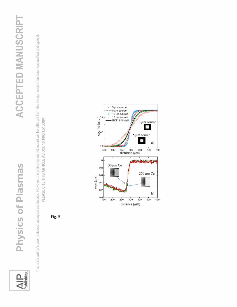
the mesh edge projections at 3, 5, 10 and 15 µm size of proton source shown in Fig. 5a) and, in inset, simulated
mesh cell radiographs at 3 and 5 µm size of proton source is shown, as an example. In Fig. 5a) the line out of
measured mesh edge projection gives the best fit, in terms of sharpness of the edges, to the simulated data for 10
µm source size, which is of the same order as the independently estimate from the ray-tracing code (Fig. 2b)).
Additionally, in order to verify the effect of possible degradation of spatial resolution of the image due to
transparency of the used 30 µm thick mesh to the e.g., 6.5. MeV protons which have stopping range of 120 µm, a
comparative study was carried out where 6.5 MeV protons were used for projection imaging of 30 µm and 250
µm thick Cu strip, shown in Fig. 5b). Mesh cell radiographs shown in inset. In simulated images for transparent
(30 µm) vs opaque (250 µm) copper meshes for 6.5 MeV protons (Fig. 5b)) the line outs of the cells edges show
Thi
s is
the
auth
or’s
pee
r re
view
ed, a
ccep
ted
man
uscr
ipt.
How
ever
, the
onl
ine
vers
ion
of r
ecor
d w
ill b
e di
ffere
nt fr
om th
is v
ersi
on o
nce
it ha
s be
en c
opye
dite
d an
d ty
pese
t.
PL
EA
SE
CIT
E T
HIS
AR
TIC
LE
AS
DO
I: 1
0.1
063/1
.5100094

7
negligible difference in sharpness, indicating that there is no additional degradation of the image due to the
transparency of the mesh.
Simulations and modelling
Particle-in-cell simulations. In the 2D PIC simulations, based on the code EPOCH [29], a 𝑝-polarized, 30 fs laser
pulse with a Gaussian profile (temporal and spatial) at 𝜆 =0.8 µ𝑚 wavelength is focused into a 4 m spot, having
normalised vector potential 𝑎0 =7, under 30 on a 1 µ𝑚 thick 𝐴𝑙4+ target with 90 nm 𝐻+ contaminant layers on
both sides. These are the parameters used in the experiments except of target thickness. A 1 m target thickness
was simulated instead of 6 m used in the experiments in order to run high-resolution simulation in reasonable
time slot. Also, there are experimental evidences that at the applied intensities here (1020 W/cm2) the target
thickness has almost no influence on maximum proton energy at optimized conditions [30]. In simulations the
initial electron temperature 𝑇𝑒 =100 eV. The target is in 𝑥𝑦 plane and 𝑧 is the target normal direction. The
simulation mesh has a size of 𝑑𝑥 = 𝜆/100 and 𝑑𝑦 = 𝜆/50 with 400 particles per cell. The target density was set
1.74×1023 cm-3 for 𝐻1+ and 6.0×1022 cm-3 for 𝐴𝑙4+. The somewhat “low” density of hydrogen contaminant layer
corresponds to the case of deposit, unstructured atomic layer of hydrogen on the target surface.
The simulation was mainly focused on reproducing the experimental findings, in particular, on virtual source
and beam properties, rather than on details not yet confirmed by the experiments. 2D PIC simulations have
reproduced the spatial characteristics of protons and revealed the details of the source and beam characteristics
far beyond the experimental limits. The momentum distribution of protons with energies from 3 MeV up to 15
MeV in phase space at a distance of 50 m from the target is shown in Fig. 6a). Here, different energy protons
have acquired different transverse momenta which stays unchanged during their further propagation.
The temporal evolution of protons momentum at an early stage of propagation exemplified for 4, 8 and
12 MeV protons in Figs. 6 b) and c). Up to about 400 fs, there is a rapid increase of all particles transverse
momentum before it saturates and bunches start to expand linearly after 400 fs due to the particles time-of-flight
(TOF) (Fig. 6b). This somehow contradicts the assumption of ballistic propagation of proton beam made in
reconstructing the virtual source of protons. The transverse momentum change of the particles during propagation
has direct impact on the “virtual source” position and size. This finding, however, does not affect the concept of
“virtual source” defined from the linear expansion part of the beam and its importance for applications.
The longitudinal momentum gain for different energy protons takes place differently (Fig. 6c)). The high
energy protons gain longitudinal momentum for much longer time than the low energy once, e.g., in Fig. 6c)
shown that the momentum of 8 MeV and 12 MeV protons increases during 300 fs and 400 fs after acceleration,
Thi
s is
the
auth
or’s
pee
r re
view
ed, a
ccep
ted
man
uscr
ipt.
How
ever
, the
onl
ine
vers
ion
of r
ecor
d w
ill b
e di
ffere
nt fr
om th
is v
ersi
on o
nce
it ha
s be
en c
opye
dite
d an
d ty
pese
t.
PL
EA
SE
CIT
E T
HIS
AR
TIC
LE
AS
DO
I: 1
0.1
063/1
.5100094

8
respectively, and 4 MeV protons start to expand linearly by TOF after 100 fs. This changes the longitudinal
emittance of the beam and needs to be taken into account at time resolved measurements. The dynamics of electric
field profiles in the vicinity of the beams (Fig. 7) shows that the transverse electric field (𝐸𝑥) at any time step is
much weaker as compared to longitudinal field (𝐸𝑧). Moreover, there is almost no transverse electric field at the
centre of the beams. Therefore, at the centre the beams profile is fully conserved. However, even small transverse
electric field at the outer part of the beams results in the progressive displacement of beamlets in a transverse
direction as measured in the experiments for outer region of the mesh images. The particles are gaining additional
forward momentum mainly from longitudinal electric field (𝐸𝑧), as shown Fig. 6c).
Fig. 8a) shows simulated “virtual source” size and position in front of the target at different proton energies
from the particles final momentum values, as it is reconstructed from the experimental mesh images (see Fig. 2).
It calculates mean and standard deviation of the particle position until the smallest standard deviation is reached.
The virtual source size is gradually decreases and moves asymptotically towards to the target surface with
increasing particles’ energy. The “virtual source” of protons above 13 MeV is located on the target surface with
a size comparable to the laser spot size, which may suggest that the “virtual source” becomes a real source on the
target front. When the rapid increase of particles transverse momentum at early time (<400 fs, Fig. 6b) is
considered, the “virtual source” will be even smaller and become located on the target surface at even for lower
proton energies (about 10 MeV).
It is interesting to note that the simulated virtual source size of protons with energy less than 5 MeV in Fig.
8a) corresponds to the virtual source size of TNSA protons (Fig. 3, “distorted image”).
The simulated 1D proton image of the mesh at a distance of 4 cm from the target by 4 MeV and 9 MeV proton
beams shown in Fig. 8b). Despite of simulated large difference in the divergences of chosen proton beams (Fig.
6a)), the mesh image is similarly reproduced by these two beams. Hence, their partial divergence is the same. The
latter agrees well with the experimental findings.
Theoretical modelling. The laser ponderomotive force pushes the hot electrons from the focal spot region deep
into a target in the form of moving electron density spike [19]. This produces an electron cavity at the target front
with a radius close to the laser focal spot radius and the hot electrons propagate along the normal to the surface of
this charged cavity. It constitutes the lower limit of the proton source size and the divergence of hot electrons.
This is in contrast to the longer laser pulses (0.4 and 1 ps) where electrons have rather large divergence [31] and
proton source size is much larger than the laser focal spot size. Adopting the theoretical model [32] based on
adiabatic energy transfer between the hot electrons and ions, the hot electron density 𝑛𝑒 as a function of the
Thi
s is
the
auth
or’s
pee
r re
view
ed, a
ccep
ted
man
uscr
ipt.
How
ever
, the
onl
ine
vers
ion
of r
ecor
d w
ill b
e di
ffere
nt fr
om th
is v
ersi
on o
nce
it ha
s be
en c
opye
dite
d an
d ty
pese
t.
PL
EA
SE
CIT
E T
HIS
AR
TIC
LE
AS
DO
I: 1
0.1
063/1
.5100094

9
potential 𝜑 of charge displacement field behind the charge cavity can be obtained from the adiabatic equation: 𝜂𝑒 = 1 + |𝑒|𝜑 2𝑇𝑒0⁄ , 𝜂𝑒 = 𝑛𝑒 𝑛𝑒𝑜⁄ . We suppose a temporal evolution of transvers profile of hot electron charge
density 𝜂(𝜉. 𝑡) results from the normalized transverse scale of the hot electrons at the rear of charge cavity (𝑙(𝑡) =𝐿(𝑡)/𝑟𝐷), which means 𝜂(𝜉. 𝑡)= 𝜂(𝜉. 𝑙(𝑡)). Compared to [32], the Lorenz distribution was considered: 𝜍 = 3/[1 +(3𝜉/𝑙)2], which is close to the simulations, for the longitudinal charge density profile of hot electron density spike
behind the charge cavity instead of delta function used in [32] for the rear of the target, and the dynamic of electric
field was determined. From the Poisson equation 𝜂𝑒(𝜉. 𝜍, 𝑙(𝑡)) is deduced.
The equations of ion motion in the charge separation field can be written as: 𝜕2𝜍𝜕𝜏2 = 𝛿 𝜕𝜓𝜕𝜍 , 𝜕2𝜉𝜕𝜏2 = 𝛿 𝜕𝜓𝜕𝜉 (2)
where 𝛿 = 𝑚𝑒/𝑚𝑖, 𝜍 = 𝑧/𝑟𝐷, 𝜉 = 𝑦/𝑟𝐷 are the coordinates normalized to the Debye radius of hot electrons 𝑟𝐷 = √𝑇𝑒0/4𝜋𝑒2𝑛𝑒0, 𝑇𝑒0 and 𝑛𝑒0 their initial temperature and density, 𝜓 = |𝑒|𝜑/𝑇𝑒0. The solution gives the
angle of ion departure for the given profile of charge distribution: 𝜃(𝜉0) = �̇�|𝜏→∞ / 𝜍̇|𝜏→∞ (3)
Eq. (3) is calculated describing the speed components in terms of field components: transverse and longitudinal
in respect to the foil surface, taking into account linear trajectories of ion, according to numerical calculations:
𝜃(𝜉0) = 𝜕𝜉 𝜕𝜏⁄ |𝜏→∞𝜕𝜍 𝜕𝜏⁄ |𝜏→∞ ≈ ∫ 𝐸𝜂(𝜉𝑜, 𝜈𝑖(𝜉𝑜)𝜏; 𝑙(𝜏))𝑑𝜏∞0∫ 𝐸𝜉(𝜉𝑜, 𝜈𝑖(𝜉𝑜)𝜏; 𝑙(𝜏))𝑑𝜏∞0 (4)
where 𝜈𝑖 - effective collision frequency, 𝐸𝜂,𝜉(𝜉, 𝜍; 𝑙(𝜏)) = −2𝜕𝜂𝑒(𝜉, 𝜍; 𝑙(𝜏))/𝜕(𝜉, 𝜂) are the tangential and
normal component of the electric field in respect to the foil surface. To calculate the angle at large distance from
the target in the solution of Poisson equation for 𝜂𝑒(𝜉. 𝜍, 𝑙(𝑡)) we substitute the Bessel function with its asymptotic
value at 𝜍 > 1 and calculate this integral by the method of steepest descend. We get: 𝜃 ≈ √2 1𝜂 𝜕𝜂/𝜕𝜉. The
maximum speed accumulated by an ion at the coordinate 𝜉𝑜 is determined by the maximal value of the non-
stationary potential in this point. Fig. 9 shows accelerated proton beam divergence at different laser intensities
calculated at zero initial speed of the particles at any starting position 𝜉𝑜. Here, for comparison, the simulation
results from Fig. 6a) for different laser intensities are plotted which is in a good agreement with calculations.
Discussions and conclusions
It has been experimentally demonstrated that energetic protons have been accelerated together in the strong
charge-separation field from a “point-size source” with a similar partial divergence in a broad energy range. These
findings suggest that a bipolar charge structure, i.e. electron cavity and electron spike is formed from the
Thi
s is
the
auth
or’s
pee
r re
view
ed, a
ccep
ted
man
uscr
ipt.
How
ever
, the
onl
ine
vers
ion
of r
ecor
d w
ill b
e di
ffere
nt fr
om th
is v
ersi
on o
nce
it ha
s be
en c
opye
dite
d an
d ty
pese
t.
PL
EA
SE
CIT
E T
HIS
AR
TIC
LE
AS
DO
I: 1
0.1
063/1
.5100094

10
interaction of high intensity, high contrast and short laser pulse with a solid target which produces a strong
accelerating field where protons are accelerated to high energy. This scenario makes possible forward acceleration
of protons from a “point-size source” for a short time, which leads to a similar partial divergence of a beams at
different energies. The simulations confirmed that the protons beams profile at the centre is fully conserved,
because the transverse electric field (𝐸𝑥) at any time step during the acceleration is much weaker as compared to
longitudinal field (𝐸𝑧) and, moreover, there is almost no transverse electric field at the centre of the beams. This
is in contrast to protons accelerated in the TNSA regime, which have relatively larger “virtual source” size. The
cavity–spike accelerated protons normalized emittance was estimated to be ε𝑛𝑡 0.065 π mm mrad. The
experimental results and simulations qualitatively agree that the “virtual source” located close to the target front
moves towards to the target and the size is gradually decreasing with increasing particles energy (Fig. 8a). There
is clear experimental evidence confirmed by simulations that the “virtual source” of high energy protons gradually
moves close to the target and, according to simulations, the “virtual source” of protons above 13 MeV, in this
case, located on the target front surface with a size comparable to the laser spot size. The latest may suggest that
the “virtual source” becomes a real source on the target front, verifying the concept of the limit of the source size.
These phenomena have not been previously considered. In contrast, the protons accelerated in TNSA regime have
a relatively larger “virtual source” and emits protons in the low energy part of the spectra. Applied analytical
model based on adiabatic energy transfer between the hot electrons and ions agrees well with simulations on
proton beam divergence change with particles energy at these conditions. However, the adiabatic approach might
be too “ideal” and some more considerations would be required taking into account the results of further
experiments.
The “virtual source” behaviour, its size and beam properties are crucial for applications dealing with beam
quality, beam transport or focusing. For instance, in radiography applications, the existence of two sources of
protons, and/or moving virtual source may produce an image of the object with features which doesn’t correspond
to the structure of the object in the object plane. A consequence is that it becomes very complex, and might be
impossible to reconstruct the object by image inversion due to the complex features of the source.
Acknowledgements
This work was performed under the ELI-ALPS Project (No. GINOP–2.3.6–15–2015–00001), supported by EU
and co-financed by the European Regional Development fund, T. W. Jeong for the support during the experiments.
S. T.-A. thanks V. Yu. Bychenkov for the thoughtful discussions.
Thi
s is
the
auth
or’s
pee
r re
view
ed, a
ccep
ted
man
uscr
ipt.
How
ever
, the
onl
ine
vers
ion
of r
ecor
d w
ill b
e di
ffere
nt fr
om th
is v
ersi
on o
nce
it ha
s be
en c
opye
dite
d an
d ty
pese
t.
PL
EA
SE
CIT
E T
HIS
AR
TIC
LE
AS
DO
I: 1
0.1
063/1
.5100094

11
Figure captures
Fig.1. Experimental setup. Laser accelerated proton imaging of the mesh on a stack of radio-chromic-film
(RCF) detector.
Fig. 2. a) Mesh images created by protons with energies above 5 MeV, e.g., 6.5, 7.3, 8.1 and 8.9 MeV. b). Ray-
tracing of the mesh image of 6.5 MeV proton beam to the “virtual source” and the zoomed source projections on
(𝑥𝑧) and (𝑦𝑧) planes. The target between the “virtual source” and the mesh is not shown in order do not overload
the picture.
Fig. 3. Typical mesh image created by protons with energies below 5 MeV, e.g., 3.1 MeV on the left. On the
right is the zoomed picture of the central part of the mesh.
Fig. 4. The measured “virtual source” size of protons at different energies shown in Fig. 2 and 3. The existence
of two distinct different virtual sources is apparent.
Fig. 5. a) Line out of the edge projections at 3, 5, 10 and 15 µm size of proton source simulated by G4beamline
code and measured in the experiment. Inset, mesh cell radiographs at 3 and 5 µm proton source. b) Line out of
the edge projections simulated by G4beamline code for 30 µm and 250 µm thick 𝐶𝑢 mesh. Mesh cell
radiographs shown in inset.
Fig. 6. a) The momentum distribution of protons for different energies at 50 m far from the target. b) The
transverse momentum changes and c) the longitudinal expansion of 4 MeV, 8 MeV and 12 MeV protons during
the propagation.
Fig. 7. The temporal evolution of longitudinal (upper row) and transvers (lower row) electric fields created by
electron cloud around 4 MeV, 8 MeV and 12 MeV proton beams.
Fig. 8. a) Simulated “virtual source” size and its distance from the target for protons with energies from 3 MeV
up to 13 MeV is ray-traced from their final momentum value. b) A simulated 1D image of the mesh, positioned
in a distance of 5 mm from the target, created by 4 MeV and 9 MeV protons at 4 cm distance from the target.
Fig. 9. Polychromatic proton beam divergence calculated at different laser intensities and simulated in Fig.3a).
Thi
s is
the
auth
or’s
pee
r re
view
ed, a
ccep
ted
man
uscr
ipt.
How
ever
, the
onl
ine
vers
ion
of r
ecor
d w
ill b
e di
ffere
nt fr
om th
is v
ersi
on o
nce
it ha
s be
en c
opye
dite
d an
d ty
pese
t.
PL
EA
SE
CIT
E T
HIS
AR
TIC
LE
AS
DO
I: 1
0.1
063/1
.5100094

12
References
1. P. K. Patel, A. J. Mackinnon, M. H. Key, T. E. Cowan, M. E. Foord, M. Allen, D. F. Price, H. Ruhl, P.
T. Springer, and R. Stephens, Phys. Rev. Lett. 91, 125004 (2003).
2. K. W. D. Ledingham, P. McKenna, and R. P. Singhal, Science. 300, 1107 (2003).
3. E. Lefebvre, E. D’Humières, S. Fritzler, and V. Malka, J. Appl. Phys. 100, 113308 (2006).
4. M. Borghesi, A. Schiavi, D. H. Campbell, M. G. Haines, O. Willi, A. J. MacKinnon, L. A. Gizzi, M.
Galimberti, R. J. Clarke and H. Ruhl, Plasma Phys. Control. Fusion. 43, A267 (2001).
5. M. Borghesi, D. H. Campbell, A. Schiavi, M. G. Haines, O Willi, A. J. MacKinnon, P. Patel, L. A. Gizzi,
M. Galimberti, R. J. Clarke, F. Pegoraro, H. Ruhl, and S. Bulanov, Phys. Plasmas. 9, 2214 (2002).
6. J. Denavit, Phys. Rev. Lett. 69, 3052 (1992).
7. A.Maksimchuk, S.Gu, K.Flippo, D. Umstadter, and V. Yu. Bychenkov, Phys. Rev. Lett. 84, 4108 (2000).
8. O. Shorokhov, and A. Pukhov, Laser Part. Beams 22, 175 (2004).
9. R. A. Snavely, M. H. Key, S. P. Hatchett, T. E. Cowan, M. Roth, T. W. Phillips, M. A. Stoyer, E. A.
Henry, T. C. Sangster, M. S. Singh, S. C. Wilks, A. MacKinnon, A. Offenberger, D. M. Pennington, K.
Yasuike, A. B. Langdon, B. F. Lasinski, J. Johnson, M. D. Perry, and E. M. Campbell, Phys. Rev. Lett.
85, 2945 (2000).
10. M. Zepf, E. L. Clark, K. Krushelnick, F. N. Beg, C. Escoda, A. E. Dangor, M. I. K. Santala, M. Tatarakis,
I. F. Watts, P. A. Norreys, R. J. Clarke, J. R. Davies, M. A. Sinclair, R. D. Edwards, T. J. Goldsack, I.
Spencer and K. W. D. Ledingham, Phys. Plasmas 8, 2323 (2001).
11. G. S. Sarkisov, P. Leblanc, V.V. Ivanov, Y. Sentoku, V. Yu. Bychenkov, K. Yates, P. Wiewior, D. Jobe,
and R. Spielman, Appl. Phys. Lett. 99, 131501 (2011);
12. A. J. Mackinnon, Y. Sentoku, P. K. Patel, D. W. Price, S. Hatchett, M. H. Key, C. Andersen, R. Snavely,
and R. R. Freeman, Phys. Rev. Lett. 88, 215006 (2002).
13. J. S. Green, N. Booth, R. J. Dance, R. J. Gray, D. A. MacLellan, A. Marshall, P. McKenna, C. D. Murphy,
C. P. Ridgers, A. P. L. Robinson, D. Rusby, R. H. H. Scott and L. Wilson, Sci. Reports 8, 4525 (2018)
14. T. Nakamura, K. Mima, S. Ter-Avetisyan, M. Schnürer, T. Sokollik, P. V. Nickles, and W. Sandner,
Phys. Rev. E 77, 036407 (2008).
15. M. Borghesi, A. J. Mackinnon, D. H. Campbell, D. G. Hicks, S. Kar, P. K. Patel, D. Price, L. Romagnani,
A. Schiavi, and O. Willi, Phys. Rev. Lett. 92, 055003 (2004).
16. S. C. Wilks, A. B. Langdon, T. E. Cowan, M. Roth, M. Singh, S. Hatchett, M. H. Key, D. Pennington,
A. MacKinnon, and R. A. Snavely, Phys. Plasmas 8, 542 (2001).
Thi
s is
the
auth
or’s
pee
r re
view
ed, a
ccep
ted
man
uscr
ipt.
How
ever
, the
onl
ine
vers
ion
of r
ecor
d w
ill b
e di
ffere
nt fr
om th
is v
ersi
on o
nce
it ha
s be
en c
opye
dite
d an
d ty
pese
t.
PL
EA
SE
CIT
E T
HIS
AR
TIC
LE
AS
DO
I: 1
0.1
063/1
.5100094

13
17. S. Ter-Avetisyan, M. Schnürer, P. V. Nickles, W. Sandner, M. Borghesi, T. Nakamura, and K. Mima,
Phys. Plasmas 17, 063101 (2010)
18. S. Ter-Avetisyan, M. Schnürer, P. V. Nickles, W. Sandner, T. Nakamura, and K. Mima, Phys. Plasmas
16, 043108 (2009).
19. V. Yu. Bychenkov, P. K. Singh, H. Ahmed, K. F. Kakolee, C. Scullion, T. W. Jeong, P. Hadjisolomou,
A. Alejo, S. Kar, M. Borghesi, and S. Ter-Avetisyan, Phys. Plasmas. 24, 010704 (2017).
20. S. C. Wilks, W. L. Kruer, M. Tabak, and A. B. Langdon, Phys. Rev. Lett. 69, 1383 (1992).
21. S. X. Luan, Wei Yu, M. Y. Yu, G. J. Ma, Q. J. Zhang, Z. M. Sheng, and M. Murakami, Phys. Plasmas.
18, 042701 (2011).
22. A. A. Andreev, R. Sonobe, S. Kawata, S. Miyazaki, K. Sakai, K. Miyauchi, T. Kikuchi, K. Platonov and
K. Nemoto, Plasma Phys. Contr. Fusion 48, 1605 (2006).
23. V. M. Ovchinnikov, D. W. Schumacher, M. McMahon, E. A. Chowdhury, C. D. Chen, A. Morace, and
R. R. Freeman, Phys. Rev. Lett. 110, 065007 (2013).
24. T. J. Yu, S. K. Lee, J. H. Sung, J. W. Yoon, T. M. Jeong, and J. Lee, Opt. Express 20, 10807 (2012).
25. J. Schreiber, S. Ter-Avetisyan, E. Risse, M. P. Kalachnikov, P. V. Nickles, W. Sandner, U. Schramm,
D. Habs, J. Witte, and M. Schnürer, Phys. Plasmas 13, 033111 (2006).
26. S. Ter-Avetisyan, L.Romagnani, M, Borghesi, M. Schnürer, and P. V. Nickles, Nucl. Instrum. Meth. A
623, 709 (2010).
27. G. Golovin, S. Banerjee, C. Liu, S. Chen, J. Zhang, B. Zhao, P. Zhang, M. Veale, M. Wilson, P. Seller
and D. Umstadter, Sci. Rep. 6, 24622 (2016).
28. https://muonsinc.com/muons3/g4beamline/G4beamline
29. T. D. Arber, K. Bennett, C. S. Brady, A. Lawrence-Douglas, M. G. Ramsay, N. J. Sircombe, P. Gillies,
R. G. Evans, H. Schmitz, and A. R. Bell, Plasma Phys. Control. Fusion 57, 113001 (2015).
30. S. Ter-Avetisyan, P. K. Singh, K. F. Kakolee, H. Ahmed, T. W. Jeong, C. Scullion, P. Hadjisolomou,
M. Borghesi and V. Yu. Bychenkov, Nucl. Instrum. Meth. A 909 156 (2018).
31. R. B. Stephens, R. A. Snavely, Y. Aglitskiy, F. Amiranoff, C. Andersen, D. Batani, S. D. Baton, T.
Cowan, R. R. Freeman, T. Hall, S. P. Hatchett, J. M. Hill, M. H. Key, J. A. King, J. A. Koch, M. Koenig,
A. J. MacKinnon, K. L. Lancaster, E. Martinolli, P. Norreys, E. Perelli-Cippo, M. Rabec Le Gloahec, C.
Rousseaux, J. J. Santos, and F. Scianitti, Phys. Rev. E 69, 066414 (2004).
32. A. Andreev, T. Ceccotti, and A. Levy, K. Platonov and Ph. Martin, New J. Phys. 12, 045007 (2010).
Thi
s is
the
auth
or’s
pee
r re
view
ed, a
ccep
ted
man
uscr
ipt.
How
ever
, the
onl
ine
vers
ion
of r
ecor
d w
ill b
e di
ffere
nt fr
om th
is v
ersi
on o
nce
it ha
s be
en c
opye
dite
d an
d ty
pese
t.
PL
EA
SE
CIT
E T
HIS
AR
TIC
LE
AS
DO
I: 1
0.1
063/1
.5100094

Fig. 1.
Thi
s is
the
auth
or’s
pee
r re
view
ed, a
ccep
ted
man
uscr
ipt.
How
ever
, the
onl
ine
vers
ion
of r
ecor
d w
ill b
e di
ffere
nt fr
om th
is v
ersi
on o
nce
it ha
s be
en c
opye
dite
d an
d ty
pese
t.
PL
EA
SE
CIT
E T
HIS
AR
TIC
LE
AS
DO
I: 1
0.1
063/1
.5100094

Fig. 2.
a)
b)
Thi
s is
the
auth
or’s
pee
r re
view
ed, a
ccep
ted
man
uscr
ipt.
How
ever
, the
onl
ine
vers
ion
of r
ecor
d w
ill b
e di
ffere
nt fr
om th
is v
ersi
on o
nce
it ha
s be
en c
opye
dite
d an
d ty
pese
t.
PL
EA
SE
CIT
E T
HIS
AR
TIC
LE
AS
DO
I: 1
0.1
063/1
.5100094

3.1 MeV
Fig. 3.
Thi
s is
the
auth
or’s
pee
r re
view
ed, a
ccep
ted
man
uscr
ipt.
How
ever
, the
onl
ine
vers
ion
of r
ecor
d w
ill b
e di
ffere
nt fr
om th
is v
ersi
on o
nce
it ha
s be
en c
opye
dite
d an
d ty
pese
t.
PL
EA
SE
CIT
E T
HIS
AR
TIC
LE
AS
DO
I: 1
0.1
063/1
.5100094

Fig. 4.
3 4 5 6 7 8 9
10
20
30
40
50
60
virtu
al sourc
e s
ize (
m)
proton energy (MeV)
Thi
s is
the
auth
or’s
pee
r re
view
ed, a
ccep
ted
man
uscr
ipt.
How
ever
, the
onl
ine
vers
ion
of r
ecor
d w
ill b
e di
ffere
nt fr
om th
is v
ersi
on o
nce
it ha
s be
en c
opye
dite
d an
d ty
pese
t.
PL
EA
SE
CIT
E T
HIS
AR
TIC
LE
AS
DO
I: 1
0.1
063/1
.5100094
450 500 550 600 650 700 750
0.0
0.4
0.8
3 m source
5 m source
10 m source
15 m source
RCF; 6.5 MeV
counts
(a. u.)
distance (m)
5 µm source
a)
3 µm source
250 µm Cu
30 µm Cu
b)
distance (m)
cou
nt
(a.
u.)
Fig. 5.
Thi
s is
the
auth
or’s
pee
r re
view
ed, a
ccep
ted
man
uscr
ipt.
How
ever
, the
onl
ine
vers
ion
of r
ecor
d w
ill b
e di
ffere
nt fr
om th
is v
ersi
on o
nce
it ha
s be
en c
opye
dite
d an
d ty
pese
t.
PL
EA
SE
CIT
E T
HIS
AR
TIC
LE
AS
DO
I: 1
0.1
063/1
.5100094

Fig. 6.
a)4
6 8 1012
MeV
14
0.07 0.11 0.15 0.19𝑝𝑧 (𝑚𝑒𝑐)
0.05
-0.05
0𝑝 𝑥(𝑚 𝑒𝑐)
1334 MeV 8 MeV 12 MeV
240 453 666 880 𝑓𝑠
0.05
-0.05
0
0 10 20 30 40𝑧 (µm)
𝑝 𝑥(𝑚 𝑒𝑐)
b)4MeV
8MeV
12MeV
0 200 400 600 800time (fs)
longit
udin
alb
eam
siz
e(µ
m) 1.5
0
0.5
1
c)
Thi
s is
the
auth
or’s
pee
r re
view
ed, a
ccep
ted
man
uscr
ipt.
How
ever
, the
onl
ine
vers
ion
of r
ecor
d w
ill b
e di
ffere
nt fr
om th
is v
ersi
on o
nce
it ha
s be
en c
opye
dite
d an
d ty
pese
t.
PL
EA
SE
CIT
E T
HIS
AR
TIC
LE
AS
DO
I: 1
0.1
063/1
.5100094

Fig. 7.
𝐸𝑧
𝐸𝑥
𝐸𝑧
𝐸𝑥
𝐸𝑧 4 MeV8 MeV
12 MeV
𝐸𝑥 4 MeV8 MeV
12 MeV
93 fs 211 fs 328 fs
10
0
-10
5
-5
𝑥(µm)
10
0
-10
5
-5
𝑥(µm)
0.2
0
-0.20.2
0
-0.210 15 20 25 10 20 30 4030 10 20 30 40𝑧 (µm) 𝑧 (µm) 𝑧 (µm)
Thi
s is
the
auth
or’s
pee
r re
view
ed, a
ccep
ted
man
uscr
ipt.
How
ever
, the
onl
ine
vers
ion
of r
ecor
d w
ill b
e di
ffere
nt fr
om th
is v
ersi
on o
nce
it ha
s be
en c
opye
dite
d an
d ty
pese
t.
PL
EA
SE
CIT
E T
HIS
AR
TIC
LE
AS
DO
I: 1
0.1
063/1
.5100094

Fig. 8.
3 MeV
4 MeV
5 MeV
target surface 13 MeV. . .
vir
tual
so
urc
e p
osi
tion
μm
pro
ton d
ensi
ty (
no
rmal
ized
)
0.4
0.8
1.2
b)
-0.5 0 0.5 1 1.5𝑥 (cm)-1-1.5𝑥 (cm)
-20 40200
-40
0
-120
-80
a)
-40
4 MeV9 MeV
Thi
s is
the
auth
or’s
pee
r re
view
ed, a
ccep
ted
man
uscr
ipt.
How
ever
, the
onl
ine
vers
ion
of r
ecor
d w
ill b
e di
ffere
nt fr
om th
is v
ersi
on o
nce
it ha
s be
en c
opye
dite
d an
d ty
pese
t.
PL
EA
SE
CIT
E T
HIS
AR
TIC
LE
AS
DO
I: 1
0.1
063/1
.5100094

Fig. 9.
1 10
100
101
102 1019 W/cm2 calculation
1020 W/cm2 calculation
1021 W/cm2 calculation
1020 W/cm2 simulation
whole
beam
div
erg
ence
proton energy (MeV)
Thi
s is
the
auth
or’s
pee
r re
view
ed, a
ccep
ted
man
uscr
ipt.
How
ever
, the
onl
ine
vers
ion
of r
ecor
d w
ill b
e di
ffere
nt fr
om th
is v
ersi
on o
nce
it ha
s be
en c
opye
dite
d an
d ty
pese
t.
PL
EA
SE
CIT
E T
HIS
AR
TIC
LE
AS
DO
I: 1
0.1
063/1
.5100094