cern-thesis-2016-010 · 2016-03-03 · iv abstract this thesis presents inclusive spectra of the...
TRANSCRIPT

CER
N-T
HES
IS-2
016-
010

Uniwersytet WarszawskiWydział Fizyki
Zakład Cząstek i Oddziaływań Fundamentalnych
Energy dependence of negatively charged pionproduction in proton-proton interactions at the
CERN SPS
Rozprawa doktorska
Mgr Antoni Aduszkiewicz
Promotor:
Prof. dr hab. Wojciech Dominik
Warszawa, sierpień 2015


Acknowledgements
I would like to thank to people who helped me and contributed in completing thiswork.
Prof. dr hab. Wojciech Dominik and Prof. dr hab. Marek Gaździcki for a uniqueopportunity to participate in the NA61/SHINE experiment at CERN, for supervi-sion of my work, inspiration and helpful ideas.
Dr Peter Seyboth and dr hab. Katarzyna Grebieszkow for weekly discussionsand numerous helpful comments.
Dr Maja Maćkowiak-Pawłowska and Szymon Puławski for joint work, fruitfuldiscussions and exchange of the experience.
Magdalena Kuich for valuable remarks and practical help.My parents and sister for never ending support.Project financed by Narodowe Centrum Nauki based on decision DEC-2012/
05/N/ST2/02759, Europejski Fundusz Społeczny and the State Budget under “Zin-tegrowany Program Operacyjnego Rozwoju Regionalnego”, Działania 2.6 “Region-alne Strategie Innowacyjne i transfer wiedzy” project of Mazowieckie voivodship“Mazowieckie Stypendium Doktoranckie”.
iv
Abstract
This thesis presents inclusive spectra of the negatively charged pions producedin inelastic proton-proton interactions measured at five beam momenta: 20, 31,40, 80 and 158 GeV/c. The measurements were conducted in the NA61/SHINEexperiment at CERN using a system of five Time Projection Chambers. The nega-tively charged pion spectra were calculated based on the negatively charged hadronspectra. Contribution of hadrons other than the primary pions was removed usingEPOS simulations. The results were corrected for effects related to detection, ac-ceptance, reconstruction efficiency and the analysis technique.
Two-dimensional spectra were derived as a function of rapidity and transversemomentum or transverse mass. The spectra were parametrised by widths of the ra-pidity distributions, inverse slope parameters of the transverse mass distributions,mean transverse masses and the total pion multiplicities.
The negatively charged pion spectra in proton-proton interactions belong to abroad NA61/SHINE programme of search of the onset of deconfinement of stronglyinteracting matter in collisions of light and intermediate-size ions. Spectra fromthis thesis were compared with the pion spectra in Pb+Pb collisions at the samebeam momenta per nucleon measured by the NA49 experiment. The results, inparticular the energy dependence of the mean pion multiplicity, support the inter-pretation of the onset of deconfinement in heavy ion collisions in the SPS energyrange. However, unexpected similarities in energy dependences of the shapes of thespectra obtained in proton-proton interactions and Pb+Pb collisions are revealed.
Results presented in this thesis will serve for comparisons with other ongo-ing NA61/SHINE measurements of hadron production in p+p, Be+Be, Ar+Sc andXe+La collisions. They widely extend the numerous, but mostly not detailed, lowstatistics existing p+p data.

v
Streszczenie
Praca przedstawia inkluzywne widma pionów ujemnych produkowanychw nieelastycznych oddziaływaniach proton-proton, zmierzone dla pięciu warto-ści pędu wiązki: 20, 31, 40, 80 i 158 GeV/c. Pomiary wykonano w eksperymen-cie NA61/SHINE w laboratorium CERN, z wykorzystaniem zespołu pięciu ko-mór projekcji czasowej (TPC). Widma pionów ujemnych wyznaczono w oparciuo widma ujemnie naładowanych hadronów. Wkład hadronów innych niż piony po-chodzące z pierwotnego oddziaływania dwóch protonów usunięto przy użyciu sy-mulacji opartej o model EPOS. Wyniki poprawiono ze względu na efekty związanez detekcją, akceptacją detektora, wydajnością rekonstrukcji oraz techniką analizydanych.
Dwuwymiarowe widma wyznaczono w funkcji pospieszności oraz pędu po-przecznego i masy poprzecznej. Wyznaczono też parametry widm: szerokości roz-kładów pospieszności, parametry nachylenia rozkładów masy poprzecznej, średniemasy poprzeczne oraz całkowite krotności pionów.
Widma pionów ujemnych w oddziaływaniach proton-proton należą doprogramu NA61/SHINE poszukiwań progu na produkcję plazmy kwarkowo-gluonowej (QGP) w zderzeniach lekkich i średnich jąder. Widma zostały porów-nane z widmami pionóww zderzeniach ołów-ołów przy tych samych pędach wiązkina nukleon, zmierzonymi w eksperymencie NA49. Wyniki, w szczególności zależ-ność energetyczna całkowitej krotności pionów, potwierdzają interpretację obec-ności progu na produkcję QGP w zderzeniach ciężkich jąder w zakresie energiidostępnych w CERN SPS. Jednocześnie zauważono nieoczekiwane podobieństwow zależnościach energetycznej kształtów widm w oddziaływaniach proton-protoni zderzeniach ołów-ołów.
Wyniki przedstawione w tej pracy posłużą do porównania z innymi pomiaramiprodukcji hadronów w zderzeniach p+p, Be+Be, Ar+Sc and Xe+La w ramach trwa-jącego programu NA61/SHINE. W stosunku do licznych, lecz mało dokładnych do-stępnych dotychczas danych pochodzących z oddziaływań proton-proton, przed-stawiane tu wyniki znacznie pogłębiają szczegółowość widm ujemnych pionów.

Contents
1 Collisions of nuclei as a tool to study strongly interacting matter 11.1 High-energy nuclear collisions . . . . . . . . . . . . . . . . . . . . . . . 11.2 Quark-gluon plasma phase transition . . . . . . . . . . . . . . . . . . . 21.3 Programme of the NA61/SHINE experiment . . . . . . . . . . . . . . . 51.4 Spectra of negatively charged pions in p+p interactions . . . . . . . . 71.5 NA61/SHINE experiment and this thesis . . . . . . . . . . . . . . . . . 8
2 NA61/SHINE detector 92.1 NA49 detector and upgrades for NA61/SHINE . . . . . . . . . . . . . 92.2 SPS beam and beam monitoring . . . . . . . . . . . . . . . . . . . . . . 102.3 Liquid hydrogen target . . . . . . . . . . . . . . . . . . . . . . . . . . . 112.4 Spectrometer system . . . . . . . . . . . . . . . . . . . . . . . . . . . . 112.5 Time of Flight detectors . . . . . . . . . . . . . . . . . . . . . . . . . . . 122.6 Projectile Spectator Detector . . . . . . . . . . . . . . . . . . . . . . . . 13
3 Time Projection Chambers 143.1 History and concepts . . . . . . . . . . . . . . . . . . . . . . . . . . . . 143.2 Principle of operation . . . . . . . . . . . . . . . . . . . . . . . . . . . . 153.3 Particle identification in TPC . . . . . . . . . . . . . . . . . . . . . . . . 183.4 NA61/SHINE Time Projection Chambers . . . . . . . . . . . . . . . . . 18
3.4.1 Construction . . . . . . . . . . . . . . . . . . . . . . . . . . . . . 183.4.2 Gas system . . . . . . . . . . . . . . . . . . . . . . . . . . . . . . 213.4.3 Reconstruction of events and tracks . . . . . . . . . . . . . . . . 25
4 Monte Carlo simulation 284.1 Purpose of using simulations . . . . . . . . . . . . . . . . . . . . . . . . 284.2 Simulation of interaction and the detector response . . . . . . . . . . . 284.3 Matching of the generated particles and reconstructed tracks . . . . . 294.4 Data-based adjustments of the simulated spectra . . . . . . . . . . . . 314.5 Simulated and measured characteristics . . . . . . . . . . . . . . . . . 35
5 Characteristics of the dataset 385.1 Data acquired and used in the analysis . . . . . . . . . . . . . . . . . . 385.2 Beam characteristics . . . . . . . . . . . . . . . . . . . . . . . . . . . . . 39
5.2.1 General properties . . . . . . . . . . . . . . . . . . . . . . . . . 395.2.2 Off-time beam particles . . . . . . . . . . . . . . . . . . . . . . . 405.2.3 Beam profile and divergence . . . . . . . . . . . . . . . . . . . . 43
5.3 Target density . . . . . . . . . . . . . . . . . . . . . . . . . . . . . . . . 445.4 Reconstruction efficiency and resolution . . . . . . . . . . . . . . . . . 45

CONTENTS vii
6 Data analysis 49
6.1 Overview of the analysis procedure . . . . . . . . . . . . . . . . . . . . 49
6.2 Event selection . . . . . . . . . . . . . . . . . . . . . . . . . . . . . . . . 51
6.2.1 List of event selection criteria . . . . . . . . . . . . . . . . . . . 51
6.2.2 Elastic event rejection . . . . . . . . . . . . . . . . . . . . . . . . 53
6.2.3 Off-target interaction rejection . . . . . . . . . . . . . . . . . . . 55
6.3 Track selection . . . . . . . . . . . . . . . . . . . . . . . . . . . . . . . . 55
6.3.1 List of track selection criteria . . . . . . . . . . . . . . . . . . . 55
6.3.2 Classification of tracks due to their topology . . . . . . . . . . 58
6.3.3 Selection of high reconstruction efficiency regions . . . . . . . 59
6.3.4 Correction for beam divergence . . . . . . . . . . . . . . . . . . 60
6.3.5 Suppression of the electron tracks . . . . . . . . . . . . . . . . . 60
6.3.6 Uncorrected spectra of selected tracks . . . . . . . . . . . . . . 62
6.4 Corrections to the spectra . . . . . . . . . . . . . . . . . . . . . . . . . . 64
6.4.1 Subtraction of the off-target interactions . . . . . . . . . . . . . 64
6.4.2 Correction for contamination of hadrons other than primaryπ− mesons . . . . . . . . . . . . . . . . . . . . . . . . . . . . . . 66
6.4.3 Correction for event losses as well as track losses and trackmigration between bins . . . . . . . . . . . . . . . . . . . . . . . 67
6.4.4 Rejection of poor quality bins of the final spectra . . . . . . . . 71
6.4.5 Total correction . . . . . . . . . . . . . . . . . . . . . . . . . . . 71
6.5 Statistical and systematic uncertainties . . . . . . . . . . . . . . . . . . 71
6.5.1 Statistical uncertainties . . . . . . . . . . . . . . . . . . . . . . . 71
6.5.2 Systematic uncertainties . . . . . . . . . . . . . . . . . . . . . . 75
6.6 Cross checks of the final spectra . . . . . . . . . . . . . . . . . . . . . . 80
6.6.1 Introduction . . . . . . . . . . . . . . . . . . . . . . . . . . . . . 80
6.6.2 Symmetries of the spectra . . . . . . . . . . . . . . . . . . . . . 80
6.6.3 Comparison with existing p+p data at 32 and 158 GeV/c . . . 83
6.6.4 Comparison with existing p+p data at 12, 19 and 24 GeV/c . . 84
7 π− spectra in p+p interactions and comparisonswith Pb+Pb data and sim-ulations 87
7.1 Introduction . . . . . . . . . . . . . . . . . . . . . . . . . . . . . . . . . 87
7.2 Double differential spectra . . . . . . . . . . . . . . . . . . . . . . . . . 87
7.3 Transverse mass spectra . . . . . . . . . . . . . . . . . . . . . . . . . . . 89
7.4 Rapidity spectra . . . . . . . . . . . . . . . . . . . . . . . . . . . . . . . 91
7.5 Mean multiplicity . . . . . . . . . . . . . . . . . . . . . . . . . . . . . . 93
7.6 Comparison with simulated spectra . . . . . . . . . . . . . . . . . . . . 95
8 Summary and outlook 98
A Coordinate system and kinematic variables 100
A.1 Introduction . . . . . . . . . . . . . . . . . . . . . . . . . . . . . . . . . 100
A.2 NA61/SHINE coordinate system . . . . . . . . . . . . . . . . . . . . . . 100
A.3 Kinematic variables . . . . . . . . . . . . . . . . . . . . . . . . . . . . . 101
A.3.1 Transverse variables . . . . . . . . . . . . . . . . . . . . . . . . . 101
A.3.2 Rapidity . . . . . . . . . . . . . . . . . . . . . . . . . . . . . . . 101

viii CONTENTS
B Procedures of spectra extrapolation 104B.1 Transverse mass spectrum extrapolation . . . . . . . . . . . . . . . . . 104B.2 Rapidity spectrum extrapolation . . . . . . . . . . . . . . . . . . . . . 106
C Tabulated results 109C.1 Introduction . . . . . . . . . . . . . . . . . . . . . . . . . . . . . . . . . 109C.2 Total multiplicities and rapidity distribution properties . . . . . . . . 109C.3 Double differential spectra . . . . . . . . . . . . . . . . . . . . . . . . . 109
C.3.1 pbeam = 20 GeV/c . . . . . . . . . . . . . . . . . . . . . . . . . . . 110C.3.2 pbeam = 31 GeV/c . . . . . . . . . . . . . . . . . . . . . . . . . . . 111C.3.3 pbeam = 40 GeV/c . . . . . . . . . . . . . . . . . . . . . . . . . . . 112C.3.4 pbeam = 80 GeV/c . . . . . . . . . . . . . . . . . . . . . . . . . . . 113C.3.5 pbeam = 158 GeV/c . . . . . . . . . . . . . . . . . . . . . . . . . . 114
C.4 Rapidity spectra . . . . . . . . . . . . . . . . . . . . . . . . . . . . . . . 115C.5 Inverse slope parameter . . . . . . . . . . . . . . . . . . . . . . . . . . . 115C.6 Mean transverse mass . . . . . . . . . . . . . . . . . . . . . . . . . . . . 115
Bibliography 116

Chapter 1
Collisions of nuclei as a tool to studystrongly interacting matter
1.1 High-energy nuclear collisions
What happens during collision of ultra-relativistic nuclei? Experiments detect largenumber of produced particles. The emitted particles carry information on courseof the collision. Yet, despite studies of the high-energy nuclear collisions startedmore than 60 years ago, there are still many unknowns.
Nuclei are made of nucleons: protons (p) and neutrons (n), which are exam-ples of hadrons, particles constituting of quarks and gluons. Six known types ofquarks (and corresponding anti-quarks) form two types of hadrons: baryons (e.g.p, Λ) composed of three quarks (or three anti-quarks), and mesons (e.g. π, K) com-posed of a quark and an anti-quark. Gluons mediate in strong interactions betweenquarks. A particular feature of the strong interactions is that a quark cannot be sep-arated from a hadron. Energy spent to pull a single quark is instead used to createa new pair of a quark and an anti-quark. This process is the most basic explanationof creation of new hadrons in high-energy hadron collisions.
Processes occurring in high-energy collisions of nuclei are dominated by thestrong interactions. The theory of the strong interactions, quantum chromody-namics (QCD), explains production of hadrons with high transverse masses (mT &
2 GeV/c2, see Appendix A.3.1), which however constitute only a small fraction ofpercent of all produced particles at the energy range
√s = 5–20 GeV, considered in
this thesis [1]. Majority of hadrons, for which mT . 2 GeV/c2 originate from inter-actions with low four-momentum transfer, q. For small q, the coupling constant islarge, preventing the QCD perturbative calculations from converging in the higherorders. These interactions are called soft or non-perturbative.
An alternative to the QCD calculations is provided by models calculating sta-tistical probability of hadron production from volume occupied by the collidingnuclei, filled with high energy density. The first model was proposed by Fermi in1950 [2]. In 1965 Hagedorn found out, that temperature of matter composed ofhadrons cannot exceed TH ≈ 158 MeV [3].
A further step is a concept of quark-gluon plasma (QGP). At high energy den-sities hadrons start to overlap. The quarks and gluons, normally confined withinhadrons, form a larger object. The process is called deconfinement. As QGP ex-pands, it cools down. The moment when the inelastic interactions stop is called

2 CHAPTER 1. COLLISIONS OF NUCLEI AS A TOOL TO STUDY . . .
Figure 1.1: Two scenarios of collision of two relativistic nuclei (‘A’ and ‘B’). Theleft side of the diagram shows direct formation of hadrons in series of the stronginteractions. The right side shows creation of quark-gluon plasma phase, and sub-sequent phase transition and chemical freeze-out. Both scenarios are followed bythe hadron gas phase and final release of the produced hadrons to the detector(thermal freeze-out). Figure taken from Ref. [4].
chemical freeze-out. The produced hadrons interact with each other elastically untilthe system reaches size exceeding their mean free path. The moment when the elas-tic interactions stop is called thermal freeze-out. In the detectors we observe thesehadrons (mostly long-living π±, K, p), or products of their decays. Two scenarios:with and without QGP creation are illustrated in Fig. 1.1.
QGP and gas of individual hadrons are two distinct phases of strongly inter-acting matter. The Statistical Model of Early Stage (SMES) [5, 6] relates hadronproduction to generation of new degrees of freedom. The number of degrees offreedom is higher in QGP, as they are connected with quarks and gluons, while inthe hadron gas they are connected with hadrons. Moreover, masses of the light had-rons are primarily generated by the strong forces. Masses of the individual quarks(mu = 2 MeV, md = 5 MeV, ms = 95 MeV) are much lower than masses of hadrons(mπ−(du) = 140 MeV, mK−(su) = 494 MeV, mp(uud) = 938 MeV) [7]. SMES predicts re-sulting differences in hadron production, which find experimental confirmation, asit will be described in the next section.
1.2 Quark-gluon plasma phase transition
Figure 1.2 shows the energy dependence of selected characteristics of hadron pro-duction and spectra [8, 9]. The spectra were measured in collisions of the heavy


1.3. PROGRAMME OF THE NA61/SHINE EXPERIMENT 5
diagram might end with a critical point within the SPS energy range. Above thecritical point the transition between the phases becomes smooth.
1.3 Programme of the NA61/SHINE experiment
The NA61/SHINE experiment (SPS Heavy Ion and Neutrino Experiment, the sixty-first experiment at the CERN North Area) studies hadron production in proton-proton, proton-nucleus, nucleus-nucleus and pion-nucleus collisions. The maingoal is study of onset of deconfinement and search of critical point. This is beingachieved by measurement of the energy dependence of hadron production prop-erties in nucleus-nucleus collisions as well as p+p and p+Pb interactions. The π−
spectra in p+p collisions presented in this thesis belong to this part of the pro-gramme.
Two additional goals include:
• study of hadron production at high transversemomenta (pT of up to 4.5 GeV/c)in high statistics of p+p and p+Pb interactions at 158 GeV/c. The data com-pared with the high pT NA49 measurements of Pb+Pb collisions will allowfor better understanding of the nucleus-nucleus reactions.
• precise hadron production measurements for the neutrino and cosmic rayexperiments. The NA61/SHINE measurements of 31 GeV/c proton interac-tion with 2 cm-thick carbon target, and 90 cm-thick replica of the Tokai toKamioka experiment (T2K) target help to calculate the T2K initial neutrinoflux. The T2K analysis bases on comparison of the neutrino measurements inthe far detector, Super-Kamiokande, with their initial flux, thus the NA61/SHINE role is of crucial importance [14–17].The Pierre Auger Observatory detects cosmic rays by measuring particlesfrom atmospheric showers reaching detectors on the ground. π++C interac-tions at 158 and 350 GeV/cmeasured in NA61/SHINE allow to reduce system-atic uncertainties in simulations of the showers used to reconstruct propertiesof the initial cosmic ray particles [18,19].
NA61/SHINE aims to identify properties of the onset of deconfinement and tofind the critical point of strongly interacting matter. This requires a comprehensivescan of the whole SPS beammomentum range from 13A to 158A GeV/c (A stands forthe nucleus mass number) with light and intermediate mass nuclei. NA61/SHINEmeasures p+p, 7Be+9Be, 40Ar+45Sc, Xe+La (the choice of beam and target nucleiis dictated by technical capabilities of the ion source, and physical and chemicalproperties of the target element) and p+Pb collisions at six beam momenta with atypical number of recorded collision events of 2 · 106 at each reaction and energy.This number includes only the central collisions in which most of the nucleonsparticipated in inelastic interaction. The programme is planned to be extendedwith the Pb+Pb energy scan.
Figure 1.4 lists the datasets being recorded by NA61/SHINE for the ion pro-gram. Figure 1.5 illustrates predicted region of the phase diagram explored by thetwo-dimensional scan, including also the data collected already by NA49.
The started two-dimensional scan of collision energy and colliding nuclei sizeis mainly motivated by the observation of the onset of deconfinement in cen-tral Pb+Pb collisions at beam momenta of about 30A GeV/c by the NA49 experi-


1.4. SPECTRA OF NEGATIVELY CHARGED PIONS IN P+P INTERACTIONS 7
1.4 Spectra of negatively charged pions in p+p inter-
actions
Pions are the lightest and by far the most abundant products of the high-energynuclear collisions. Thus, data on pion production properties are crucial for con-straining basic properties of models of the strong interactions. In particular, themost significant signals of the onset of deconfinement (the “kink” and “horn”, seeFig. 1.2) [12] require precise measurements of the mean pion multiplicity at thesame beam momenta per nucleon as the corresponding A+A data. Moreover, theNA61/SHINE data are taken with almost the same detector and similar acceptanceas the NA49 Pb+Pb measurements, allowing to cancel possible systematic effectscommon to both experiments.
In the CERN SPS beam momentum range of 10–450 GeV/c the mean multiplic-ity of negatively charged pions in inelastic p+p interactions increases from about0.7 at 10 GeV/c to about 3.5 at 450 GeV/c [28]. Among three charged states of pi-ons the most straightforward measurements in the largest phase-space are usuallypossible for the π− mesons. Neutral pions can be detected only indirectly, by mea-surement of invariant mass spectrum of two photons from their decays. The lowmass NA61/SHINE detector is not well suited to detect photons; also sophisticationof the analysis procedure limits precision of the results. Charged pions can be de-tected directly by ionisation detectors as they decay weakly with a relatively longlifetime. A significant fraction of positively charged hadrons are protons (25%)and kaons (5%) [25–27]. Therefore measurements of the π+ mesons require theiridentification by measurements of the energy loss and/or time-of-flight. This iden-tification is not as crucial for the π− mesons because contribution of K− and p tothe negatively charged hadrons is below 10% [25–27] and can be estimated reliablybased on simulation. The latter method is used in this thesis and it allows to deriveπ− spectra in a broad phase-space region using a uniform analysis method.
The thesis is organised as follows. Chapter 2 describes the NA61/SHINE experi-mental set-up. A detailed description of the main detector, Time Projection Cham-bers, is given in Chapter 3. The simulation used to correct the data is describedin Chapter 4. Performance of the reconstruction and the detector is described inChapter 5. The analysis technique is described in Chapter 6. The final results arepresented in Chapter 7. The results are compared with the corresponding data oncentral Pb+Pb collisions and with Monte Carlo simulations. A summary in Chap-ter 8 closes the paper.
The appendices include definitions of the coordinate system and variables usedin the analysis (Appendix A), details on calculations used to extrapolate the data tothe non-measured regions (Appendix B) and tabulated results (Appendix C).
The thesis presents results on p+p at beam momenta of 20, 31, 40, 80 and158 GeV/c measured by the NA61/SHINE detector. The results are inclusive π−
spectra – distributions of π− produced in all inelastic p+p interactions as a func-tion of rapidity (y) and the transverse momentum (pT) as well as the transversemass (mT). These results published in a NA61/SHINE paper Ref. [29] of which Iam the principal author. This thesis describes the analysis steps in much more de-tail, extends presentation of the results and provides additional comparisons andcross-checks.

8 CHAPTER 1. COLLISIONS OF NUCLEI AS A TOOL TO STUDY . . .
1.5 NA61/SHINE experiment and this thesis
NA61/SHINE is an international collaboration, as of May 2015 numbering about150 participants and 30 institutions, including 7 institutions from Poland. Polishgroups contribute substantially to the detector operation and development, partic-ipation in data taking, data calibration and reconstruction, software developmentand conservation, simulations and analysis of particle spectra, fluctuations and cor-relations. Polish groups engage in the ion and neutrino programs.
The collaboration developed from collaboration of the NA49 experiment tak-ing data in 1994–2002. In 2003 the Expression of Interest was formulated atCERN [30]. The Letter of Intent was submitted at the beginning of 2006 [31] for the“NA49-future” experiment using modernised NA49 detector for a broad programof hadron production measurements.
I joined the experimental group in 2006 under supervision of prof. Wojciech Do-minik. Together with the initiators of the new experimental programme I partici-pated in starting and testing the detector operation the shut-down in 2003. Follow-ing the successful tests the NA61/SHINE Collaboration was established in 2007. Inthe same year the first data on p+C interactions at 31 GeV/c was taken. Year 2008was devoted for upgrade of the data acquisition system. In 2009 the p+p data atfive beam momenta were collected, starting the ongoing two-dimensional scan ofthe beam momentum and the system size.
Since the beginning I work on operation and maintenance of the gas system ofthe NA61/SHINE Time Projection Chambers (TPCs), the main tracking detector.In the subsequent years my responsibility was broadened by operation of the TPCsand coordination of the experimental group. Since 2014 I have been entrusted withthe task of NA61/SHINE deputy technical coordinator.
I worked on many levels of analysis of the p+p data presented in this thesis.From 2009 I work on calibration of the drift velocity in the TPCs for this, and sub-sequent datasets. I studied details of the simulation, in particular ambiguities inthe matching procedure. In collaboration with Agnieszka Ilnicka we developed ad-justments of the simulated spectra based on the experimental data. I cooperatedwith the NA61/SHINE Ion group in verification of validity of the data. I verifiedthe reconstruction efficiency and momentum reconstruction resolution. I studiedimpact of the event and track selection properties on the analysis results, in partic-ular the role of the off-time beam particles. Finally I developed the procedures forthe data analysis and calculations of uncertainties, as well as I compared the resultswith data from other experiments and simulations.


10 CHAPTER 2. NA61/SHINE DETECTOR
The main detector upgrades for NA61/SHINE program include a new readoutand data acquisition system, which increased the data taking rate by factor of 10(to 80 events/s), new beam position detectors, new forward ToF detector and newforward calorimeter.
The main components are briefly presented below. A separate Chapter 3 is de-voted to the TPCs. Detailed description of the NA61/SHINE beam line and detectorsystem is given in Ref. [32].
2.2 SPS beam and beammonitoring
The CERN proton acceleration chain starts with linear accelerator LINAC2, whichaccelerates protons to 50 MeV/c. Next, they are injected into BOOSTER (1.4 GeV/c),the Proton Synchrotron (25 GeV/c), and finally into the Super Proton Synchrotron(SPS). SPS serves as an injector of 450 GeV/c protons into the Large Hadron Collider,but also delivers beams to fixed target experiments. Due to practical and safetyreasons the fixed target experiments use secondary beams generated by the primary400 GeV/c protons from SPS.
The secondary beam for the H2 line used by NA61/SHINE was produced ininteractions of the primary protons with a beryllium target. The beam momentaof 20, 31, 40, 80 and 158 GeV/c were selected with a set of magnetic spectrometersand collimators. Details on the accelerator chain are given in Ref. [32, Sect. 2].
Schematic of the beam detectors is magnified on the bottom of Fig. 2.1. A pairof Cherenkov detectors: Cherenkov Differential Counters with Achromatic RingFocus [34] (labelled CEDAR) and a threshold detector (labelled THC) was used toidentify protons in the beams of momenta of 20–40 GeV/c. The number of misiden-tified beam particles is below 0.8% [32]. The beam particles were detected withtwo scintillator counters, S1 and S2, centred on the beam line. The large (6×6 cm2)S1 counter defines the time reference for the detector. The small (∅ = 2.8 cm) S2counter, and a set of counters with holes centred on the beam axis (V0, ∅ = 1.0 cm;V1, ∅ = 0.8 cm and V1p, ∅ = 2.0 cm) select particles passing close to the nominalbeam axis and rejects cases of beam scattering in the beam line.
A scintillator counter S4 is located behind the target on the extrapolated beampath, taking into account deflection in the magnetic field. This counter was usedto detect interaction, as it is expected that the produced particles are unlikely tohit S4. In fact for the 80 and 158 GeV/c beams a non-negligible subclass of eventscontains a particle hitting S4. The correction for the related bias will be describedin Sect. 6.4.3. In order to ensure the interaction detection efficiently, the beam wasfocused in the S4 counter region.
Incident protons were selected by coincidence
beam ≡ S1∧ S2∧V0∧V1∧V1p ∧CEDAR∧THC . (2.1)
Positive signal from S1 and S2 counters and lack of signal from V0, V1, and V1p
counters ensures proper beam alignment. Beam protons are identified by positiveCEDAR signal, and lack of contamination of lighter particles (π±, K±) was ensuredby lack of THC signal.
Interactions of the incident beams were identified by an additional requirementof lack of the S4 signal:
interaction ≡ beam∧ S4 . (2.2)

2.3. LIQUID HYDROGEN TARGET 11
These selection criteria were applied during data collection. Simultaneously a datasample with low statistics was collected with the beam trigger only for cross-checks.
The trajectory of each beam particle was measured with three Beam PositionDetectors (BPD). They are gas detectors using Ar/CO2 85/15 mixture, consistingof two perpendicularly aligned layers of readout strips. Each layer measures co-ordinate x or y of the beam position. The measurement allows to extrapolate thebeam track to the target plane with precision of about 100 µm. For details seeRef. [32, Sect. 3.3].
2.3 Liquid hydrogen target
Liquid hydrogen was used as a proton target (LHT). The target system was usedpreviously by the NA49 experiment [25]. It is located 88.4 cm upstream of VTPC-1(target centre at z = −581 cm). The target cell was a cylinder of length of 20.29 cm(2.8% interaction length at 158 GeV/c) and 3 cm diameter. It was filled with liquidhydrogen at the pressure of 75 mbar above the air pressure. The target cell wassurrounded by vacuum in order to minimise non-target interactions and secondaryinteractions of the produced particles.
The target system allowed to insert and remove1 hydrogen from the cell. About10% of the total statistics is collected with target removed, taken 2–3 times eachday. The target removed data were used to correct for the beam interactions withthe non-target material, mainly the target cell windows (see Sect. 6.4.1).
The liquid hydrogen density equalled ρinserted ≈ 0.07 g/cm3. The density ratioof target removed (gaseous residue) to inserted was estimated to ρremoved/ρinserted ≈0.5%, see also Sect. 5.3 for detailed analysis.
2.4 Spectrometer system
Set of five Time Projection Chambers (TPCs) serves as the main spectrometer of theproduced particles. TPCs measure three-dimensional tracks of charged particles,their momentum and the charge sign and allow to identify their mass.
The five detectors of total volume of about 40 m3 are located downstream fromthe target. A detailed overview of TPCs is given in Sect. 3.
Two TPCs called Vertex TPC (VTPC) are located in the gap between upperand lower coils of two superconducting magnets: VERTEX-1 and VERTEX-2 [32,Sect. 4.3]. The magnets provide magnetic field polarised downwards (towards neg-ative values of y), uniform in majority of the detector fiducial volume. Paths of thecharged particles are bent in the horizontal plane. A detailed map of the magneticfield, including inhomogeneities measured at the VTPC corners is used to fit theparticle tracks.
The maximummagnetic field: 1.5 T in VERTEX-1 and 1.1 T in VERTEX-2 corre-sponding to 9 Tm in total, was used with the 158 GeV/c beam. The TPC acceptancewith this magnetic field setting covers the region of rapidities equal and greater
1The terms inserted and removed are used in NA61/SHINE in order to unify the naming for theliquid (e.g. hydrogen) and solid (e.g. beryllium) targets.


2.6. PROJECTILE SPECTATOR DETECTOR 13
bars of length of 120 cm, covering the total area of 8.6 m3. Each scintillatoris read by two photo-multipliers at both ends. The time difference betweenthe two signals allows to identify the hit position along the scintillator bar.The detector was used for measurements of p+p, p+C and π+C interactions,where the frequency of double hits in the scintillator bars was low due to lowtotal produced particle multiplicity.
The ToF data was not used for the data analysis presented in this thesis. How-ever the side ToFs served as a geometrical reference in calibration of the drift veloc-ity of the TPCs.
2.6 Projectile Spectator Detector
Projectile Spectator Detector (PSD) is a sampling calorimeter designed and builtfor NA61/SHINE [36]. The University of Warsaw contributed in production of thedetector. It is located behind all other detectors on the beam path. It counts thenon-interacting nucleons (spectators) of the beam nucleus by measuring their totalenergy. Such precise measurement is necessary to determine the collision centralityneeded in ion-ion collisions.
During the p+p data taking in 2009 a prototype of nine modules was tested.First physics data were obtained with detector of 36 modules in 2011; a completedetector of 44 modules was first used in 2012 to measure the Be+Be reactions.

Chapter 3
Time Projection Chambers
3.1 History and concepts
A Time Projection Chamber (TPC) is a detector of charged particles [37]. Their tra-jectories are measured in space. It was first proposed in 1976 by David Nygren andcollaborators for the PEP-4 collider experiment at SLAC. The detector was com-pleted in 1981 [38, 39]. This first TPC had volume of 6 m3 and consisted of twocylindrical drift chambers arranged around the beam pipe, with multiwire propor-tional chambers (MWPC) reading signals at the end-caps. Since then, devices of asimilar design were used in the collider experiments: 43 m3 ALEPH TPC [40] and10 m3 DELPHI TPC [41] at LEP in CERN, 49 m3 TPC of the STAR experiment atRHIC in BNL [42] and 90 m3 TPC of the ALICE experiment at LHC in CERN [43].A simpler, box-like TPCs were used in the fixed-target experiments. An exampleis the NA49 TPC system [33], later inherited and upgraded by the NA61/SHINEexperiment. It was used to collect the data analysed in this thesis and it will bedescribed in detail in this chapter.
A TPC is filled with a working medium which can be gas or liquid. Low densityof the gas allows to achieve low rate of the secondary interactions. For this reasonit is chosen typically in the accelerator experiments, as those listed above. On thecontrary, large densities of liquids allow them to serve as targets for the ultra lowcross-section interactions of neutrinos or hypothetical weakly interacting massiveparticles (WIMP). Examples include the liquid argon TPC of the ICARUS neutrinoexperiment [44] and the liquid xenon TPCs in the XENON experiment series [45].In this thesis I will consider only the gas-filled TPCs.
Figure 3.1 shows a schematic of a TPC. A field cage encloses the active volumeof a TPC, generating uniform electric field inside. Charged particles ionise the gasinside along their trajectories. Electrons (blue circles) freed in the process drift inpresence of a uniform electric field towards the readout plane. As the number ofelectrons released in gas is relatively low (several to several hundreds per cm forrelativistic particles), a charge amplification structure is located before the readoutplane. This could be a MWPC, or developed in the last years gas electron multiplier(GEM).
The electrons are registered on a two-dimensional plane of readout pixels.Charge location on the readout plane is a projection of two coordinates (x and zin NA61/SHINE) of the track. Signal on the readout pixels is sampled many timesduring the charge collection from the drift volume. Measurement of the the drift
3.2. PRINCIPLE OF OPERATION 15
R
R
R
R
R
R
R
1. primary particle ionises the gas
elec
tric
fie
ld (
dri
ft)
field cage plate
readout plane
measuredparticle
HV
Voltagedividerfor the field cage
2. electrons drift towards the readout plane
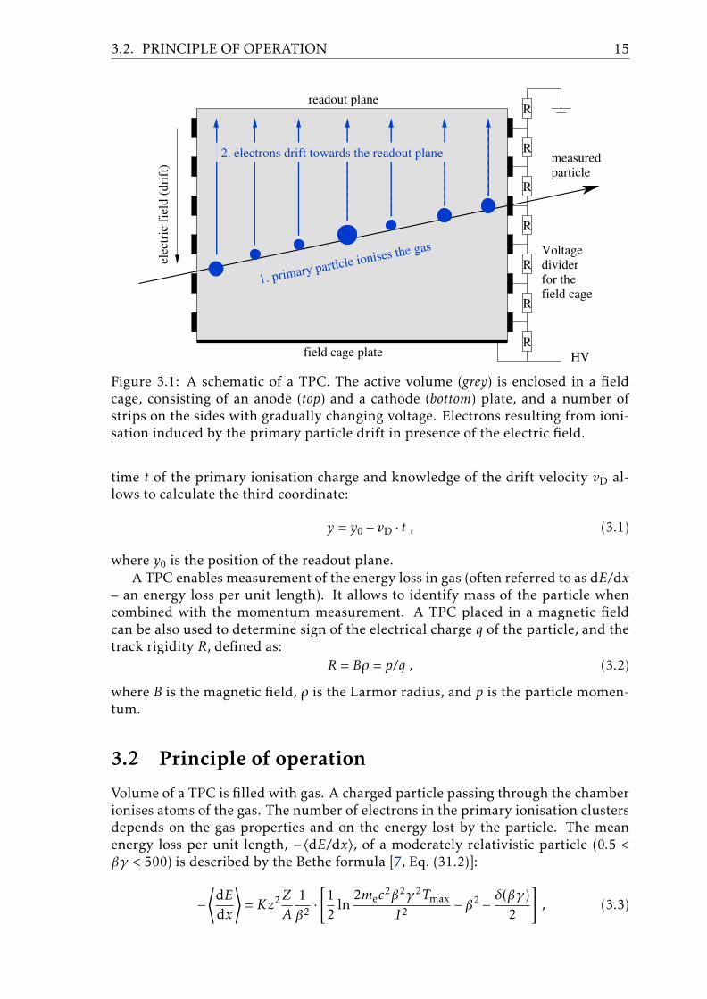
Figure 3.1: A schematic of a TPC. The active volume (grey) is enclosed in a fieldcage, consisting of an anode (top) and a cathode (bottom) plate, and a number ofstrips on the sides with gradually changing voltage. Electrons resulting from ioni-sation induced by the primary particle drift in presence of the electric field.
time t of the primary ionisation charge and knowledge of the drift velocity vD al-lows to calculate the third coordinate:
y = y0 − vD · t , (3.1)
where y0 is the position of the readout plane.A TPC enables measurement of the energy loss in gas (often referred to as dE/dx
– an energy loss per unit length). It allows to identify mass of the particle whencombined with the momentum measurement. A TPC placed in a magnetic fieldcan be also used to determine sign of the electrical charge q of the particle, and thetrack rigidity R, defined as:
R = Bρ = p/q , (3.2)
where B is the magnetic field, ρ is the Larmor radius, and p is the particle momen-tum.
3.2 Principle of operation
Volume of a TPC is filled with gas. A charged particle passing through the chamberionises atoms of the gas. The number of electrons in the primary ionisation clustersdepends on the gas properties and on the energy lost by the particle. The meanenergy loss per unit length, −〈dE/dx〉, of a moderately relativistic particle (0.5 <βγ < 500) is described by the Bethe formula [7, Eq. (31.2)]:
−⟨
dE
dx
⟩
= Kz2Z
A
1
β2·[
1
2ln
2mec2β2γ2Tmax
I2− β2 − δ(βγ)
2
]
, (3.3)

16 CHAPTER 3. TIME PROJECTION CHAMBERS
Figure 3.2: Energy loss per unit length, −〈dE/dx〉, for muons in copper. The regionrelevant for TPCs in typical high-energy physics experiments is marked by the thickblue line. The characteristic properties of this region is the decrease proportionalto 1/β2 at the low energies, a minimum at βγ ≈ 3 and a slow increase at the higherenergies. Figure taken from [46, Fig. 27.1].
where γ = (1 − β2)−1/2, β = v/c, v – velocity of the particle, c – speed of light, x –distance travelled by the particle, z – particle charge in electron units, Z – atomicnumber of absorber, A – atomic mass of absorber, me – mass of the electron, Tmax –maximum kinetic energy that can be imparted to a free electron in a single collision,I – mean excitation energy of absorber, K = 0.307075 MeV g−1cm2 (constant), δ(βγ)– density effect correction to ionization energy loss.
The formula Eq. (3.3) is a function of the particle velocity β. This dependenceis visualised in Fig. 3.2. Particles of different masses m and the same momentum phave different velocities:
β =p
mc. (3.4)
Hence, measurement of the energy loss and the momentum allows to identify massof the particle.
The formula Eq. (3.3) describes the average energy loss per unit length, howeveractual value undergoes large statistical fluctuations. The energy loss needs to bemeasured on a long path in order to provide identification power.
The readout plane is divided into pixels allowing to select short track piecescorresponding to the energy losses in thin gas layers. Distribution of the energydeposit in a track piece is often parametrised with the Landau distribution [47].An example is shown in Fig. 3.3 (left). A characteristic feature of this distributionis a long tail at the high values: occasionally the energy deposit is very large. Asa result the mean value of the energy loss along the track fluctuates strongly. Im-pact of the fluctuations can be reduced by omitting the extreme values in the meanvalue calculation. For example, in NA61/SHINE only the 50% track pieces withthe lowest energy loss is used to calculate the mean loss; this so-called truncation


3.4. NA61/SHINE TIME PROJECTION CHAMBERS 19
VTPCs MTPCs GAP TPCWidth (x) [mm] 2 000 3 900 815Length (z) [mm] 2 500 3 900 300
Number of padrows 72 90 7Drift length (y) [mm] 666 1 117 590
Drift voltage [kV] −13 −19 −10.2Drift field [V/cm] 195 170 173
Drift velocity [cm/µs] 1.4 2.3 1.4Ar/CO2 mixture 90/10 95/5 90/10
Table 3.1: Characteris-tics of the NA61/SHINETPCs: dimensions, driftvoltages, fields and ve-locities and the gas mix-ture proportions.
1 3 4 52
6 7 8 9 10
11 12 13 14 15
16 17 18 19 20
22 23 24 2521
1 3 4 52
6 7 8 9 10
11 12 13 14 15
127 (191)
16 17 18 19 20
22 23 24 2521
2 31
4 5 6
2 31
4 5 6
MtpcL
MtpcR
Vtpc2Vtpc1
Beam (z)
Jura (x)
Sector Numbers
#1 #2
#3
#4
Padrow/Pad Numbers
1 2 3 4 5 6 7 17 18 (24) Row
Pad
Beam
seen from top
(electronics side)
IC on FE boards are
on downstream side
1
2...
128 (192)
Figure 0.1: Schematic of NA49 numbering conventions5Figure 3.5: Top: NA61/SHINE TPC sector numbering convention. Bottom: Align-ment and numbering convention of the NA61/SHINE TPC padrows and padswithin a single sector. Drawing taken from [49].


3.4. NA61/SHINE TIME PROJECTION CHAMBERS 21
padrows of the GAP TPC are insufficient to reconstruct the tracks passing the GAPTPC alone. However it allows to reconstruct the tracks missing the VTPCs, whichwould otherwise leave only a straight track in one of the MTPCs.
3.4.2 Gas system
The detection properties of TPC strongly depend on the gas mixture choice [50].Firstly, the drift velocity must be sufficiently high, to allow the charge to be col-lected from the full TPC volume within the event readout period, which is 50 µs inNA61/SHINE. Although for many gas mixtures the drift velocity can be increasedin a large range by increasing the drift voltage, there are practical and safety limi-tations related to the chosen power supplies and cables, and heating of the voltagedivider resistor chain; the NA61/SHINE TPCs are operated at voltages below 20 kV.Secondly, the gas amplification must be stable. An addition of so-called quenchinggas helps to limit excessive and uncontrolled growth of the electron avalanches.
The mixtures chosen in NA49 were Ne/CO2 90/10 in VTPCs and GAP TPC andAr/CO2/CH4 90/5/5 in MTPCs, based on experimental measurements of prop-erties of various mixtures [33, 51, 52]. Argon as a base component of the MTPCgas is characterised by large number of electrons produced in the primary ionisa-tion. Lighter neon used in VTPCs and GAP TPC allowed to reduce the number ofunwanted interactions with the gas, in particular production of δ-electrons of en-ergies of fraction of GeV, which can be trapped in the magnetic field and producehigh background signals. Methane and carbon dioxide served as quenching gases.
Table 3.1 lists the gas mixtures selected in NA61/SHINE, consisting of argonand carbon dioxide only. It was verified that the detection properties with thenew mixtures satisfy the experimental requirements [53]. Absence of flammablemethane and use of more similar mixture in all TPCs facilitates the detector oper-ation and calibration of the data. The δ-electrons production was not of a concernwith the proton and pion beams used in the first years of operation. Later, beforethe first data taking period with beams of heavier ions, a helium-filled pipe centredon the beam line was introduced in the VTPCs, reducing interactions with the TPCgas by factor of about 10 [32].
Stability and purity of the gas mixture are critical for the detector operation.The drift velocity and gas amplification strongly depend on the gas content (orderof 1% change in the drift velocity per 0.1% change of the Ar/CO2 proportion).Contamination of electronegative oxygen causes charge absorption along the driftpath which is significant already at the levels of tens of ppm (parts per million).Water at the level of 100 ppm modifies the drift velocity by about 1% [33].
Gas in VTPCs and MTPCs is supplied by four independent, almost identicalsystems. Figure 3.7 presents the gas system of MTPC. The symbols used in thediagram are explained in Fig. 3.8. The fresh gas is mixed from the pure Ar andCO2 using mass flow controllers. The gas is recirculated through set of filters withrate of about 20% detector volume per hour, i.e. 0.9 m3/h for the VTPCs and and3 m3/h for the MTPCs. Only about 3% of this amount is a fresh gas.
In order to limit secondary interactions, side walls of the TPCs consist only oftwo layers of 125 µm-thick Mylar foils. The space between two foils is flushed withnitrogen to protect the gas from contamination by air due to diffusion through thewalls and in case of leak. This fragile construction could be easily damaged by ex-

22 CHAPTER 3. TIME PROJECTION CHAMBERS
G
Oxygen filter
Oxygen filter
A
A
A
A
C
Ar CO CH N2 4 2
gas
around
B
outside
D
D
V11V1
MFM
D3
p−input
V9
V12
V14
V16
V17
V15
V18
V19
V20
V20’
F.inF.out
F.B
H2 H3
PT
HUBA
bubbler
D6F.EF.DF.C
H1
F.A
D4D5
MTPC
VTPC H1’
VTPC
VTPC
MTPC
V10
A3 A4
V13
V13’
i
B3 B4
H
F2
F1
D1
(flow−rec)
(flow−sec)
D2
(bypass)
VTPC
VTPC
p−sec
big tank
small
tank
Figure 3.7: A schematic of the gas system of one of the MTPCs. The schematic forVTPCs is almost identical. The symbols used are explained in Fig. 3.8. The mainparts are drawn with bold lines; the dashed lines show connections not used in theregular operationmodes. The gas mixing system is shown in the upper right corner.The fresh gas enters the small buffer tank and then the TPC. A compressor pumpsthe gas out of the TPC and circulates it through the oxygen filter. The oxygen andwater content in the gas can be monitored in points labelled B, C, D and G. Thedrift velocity and the gas amplification can be measured in fresh gas and in gascoming from the TPC in the monitors drawn on the right side, labelled D and A,respectively.

3.4. NA61/SHINE TIME PROJECTION CHAMBERS 23
G
− exhaust (auxiliary)
A− ’A’ − amplitude measurement ’D’ − drift velocity measurement
− valve
− pressure regulator
− state valve solenoid actuator
− manometer
− flowmeter
− massflowmeter (Bronkhorst/Hi−Tec)
− compressor
− non−retour valve
− mechanical filter
− B, D, C and G points
for O and H O measurement22
Figure 3.8: Descriptions of symbols used inFig. 3.7.
cessive overpressure or underpressure of the gas in the TPC. The gas is circulatedby a compressor, which circulation speed is adjusted automatically to maintain aconstant overpressure of 0.50± 0.01 mbar in the chamber above the ambient pres-sure. The small overpressure additionally prevents contamination by air in case ofleak. Safety bubbler protects the TPC from excessive overpressure in case of thecompressor failure, or when the compressor is switched off.
The recirculated gas is flushed through a filter made of activated copper. Thefilter reduces the oxygen contamination to about 5 ppm. The water content is alsoremoved, but after about 2 weeks of operation first signs of filter saturation are vis-ible. Typically water levels of 20–100 ppm are achieved. The filters are regeneratedafter 4–6 months of operation by flushing them with the Ar/H2 (97/3) mixture at200◦C for 2–3 days. The regeneration progress is monitored by measuring moisturein the outgoing gas. An additional filter is used to remove dust from the gas.
Quality of the gas mixture is monitored periodically in a set of detectors. Fig-ure 3.9 shows example values measured in MTPC-R. For each TPC we monitor thedrift velocity vD, temperature T and drift voltage U (both in the drift monitor andin the TPC), air pressure p, and the oxygen and water content in the gas. For thegas mixtures used in NA61/SHINE, in the first approximation
vD ∼T ·Up
, (3.5)
where the T is given in Kelvin. While the temperature and the drift voltage isstabilised on a sub-permille level (panels c and d) most of the time, variations of theair pressure (panel b) change the drift velocity by several percent. The normaliseddrift velocity, corrected for changes of T , U and p allows to monitor stability of thegas mixture. Its increase visible in the panel amight be related to stability of the gasflow controllers and/or a decrease of the water level (panel e) caused by decrease ofthe air humidity in the autumn. Measurements of T and U in the TPCs allows tocalculate the drift velocity in the TPC (panel a).
The calculated values of the drift velocity are used for the first calibration recon-struction of the data (details of reconstruction will be explained in the next section).

24 CHAPTER 3. TIME PROJECTION CHAMBERS
01/10 08/10 15/10 22/10 29/10 05/11
s]
µ [
cm
/D
v
2.25
2.3
2.35
measuredDv
calculated in TPCDv
normalisedDv
(a)
01/10 08/10 15/10 22/10 29/10 05/11
p [
mb
ar]
950
960
970
(b)
01/10 08/10 15/10 22/10 29/10 05/11
C]
°T
[
16
18
20
22
24
T in TPC
T in drift monitor
(c)
01/10 08/10 15/10 22/10 29/10 05/11
E [
V/c
m]
169
170
171
E in drift monitor
E in TPC
(d)
time 2009Oct 01 Oct 08 Oct 15 Oct 22 Oct 29 Nov 05
O [
pp
m]
2 a
nd
H2
O
0
10
20
30
40 water
oxygen
(e)
Figure 3.9: Parameters of the gas inMTPC-Rmonitored in a selected period of time.a: drift velocity measured in the drift monitor, normalised based on measurementsof pressure, temperature and drift voltage, and calculated in the TPC conditions, b:air pressure, c: gas temperature in the drift monitor and in the TPC, d: electric fieldin the drift monitor and in the TPC, e: water and oxygen content in the TPC gas.


3.4. NA61/SHINE TIME PROJECTION CHAMBERS 27
fitted vertex z [cm]700− 600− 500− 400− 300−
]-1
ev
en
ts/d
z [
cm
210
310
410
510
target holder
targ
et
ce
ll
He
bo
x
air
VTPC-1
target inserted
3.69)×target removed (
Figure 3.12: Distribution of the fitted vertex z coordinate for interactions of pro-ton beam at 40 GeV/c with target inserted and removed. Peaks in the histogramreflect the distribution of the material along the beam line: liquid hydrogen, walls,vacuum, helium, and the TPC working gas.
secondary; a distinction must be done on the analysis level, for example byrestricting the impact parameter range.
Information available for each track include:
• electric charge sign,• momentum vector at the interaction vertex,• average charge loss 〈dE/dx〉,• number of points measured in each TPC,• impact parameters in the x and y coordinates, bx and by respectively.
During the analysis the events and tracks pass additional selection. Only eventscontaining interaction of the beam particle with the target are accepted. Eventswith high background from the off-time particles are rejected. Tracks are requiredto be sufficiently long and precisely fitted to the interaction point. This ensures theparameters of the particles are well measured, and that background is suppressed.While the selection criteria will be described in detail in Sects. 6.2 and 6.3 devotedto the analysis method, in the subsequent Chapters 4 and 5 describing simulationsand characteristics of the collected data I will often refer to tracks passing the se-lection criteria.
Typical spacial resolution, defined as an average distance between the pointsand tracks is several hundred µm, and two tracks distant by 1 cm can be distin-guished. The resulting momentum resolution σp/p
2 = 7.0 ·10−4 (GeV/c)−1 for tracksdetected in VTPC-1 only, and σp/p
2 = 0.3 · 10−4 (GeV/c)−1 for tracks detected inVTPC-2 and one of the MTPCs [33]. High precision of point identification withgood two-track separation allowed to reconstruct high multiplicity (>1000 tracks)Pb+Pb collisions by the NA49 experiment.

Chapter 4
Monte Carlo simulation
4.1 Purpose of using simulations
The detector properties are studied using simulations. Dedicated software usingMonte Carlo (MC) techniques simulated interactions of the beam particle with thetarget, propagation of the produced particles through the detector and processesrelated to detection.
In the analysis presented in this thesis the MC simulation is used:
• to study the detector resolution and detection properties (see Sect. 5.4),• to identify regions with good geometrical acceptance and high reconstructionefficiency (see Sect. 6.3.3),
• to correct for the detection inefficiencies and other related effects (seeSect. 6.4.3),
• to identify contributions of various charged particles among the measuredtracks (see Sects. 6.3.5 and 6.4.2).
The effects not included in the NA61/SHINE simulation yet are:
• the transmission of beam particle through the beam line including possibleinteractions outside of the target and deviation of the beam direction fromthe z axis (see Sect. 6.3.4),
• other beam particles arriving during the TPC readout (see Sect. 5.2.2),• energy loss of the produced particles (dE/dx) in the TPCs.
The following naming convention is used in this thesis. The particle spectrafrom the generator, not reconstructed nor propagated through the detector arecalled generated, and labelled with a subscript gen in formulae. The reconstructedspectra are labelled with a subscript sel, to emphasize that only tracks passing theselection criteria which will be described in Sect. 6.3 are considered. The MC sim-ulated spectra are distinguished from the data spectra by a superscript MC, or amodel name in the superscript.
4.2 Simulation of interaction and the detector response
First, an event generator simulates the initial proton-proton interaction. The eventgenerator outputs list of primary produced particles and their momenta. The short-living particles decaying via strong and electromagnetic processes also decay at the

4.3. MATCHING OF THE GENERATED PARTICLES AND . . . 29
generator level and the decay products are considered primary. The events arerandomly rotated in the x–y (transverse) plane.
Several MC models were compared with the NA61/SHINE results on p+p,p+C and π+C interactions: FLUKA2008, URQMD1.3.1, VENUS4.12, EPOS1.99,GHEISHA2002, QGSJetII-3 and Sibyll2.1 [54–57]. Based on these comparisons andtaking into account continuous support and documentation from the developersthe EPOS model [58] was selected for the MC simulation used in this thesis. TheVENUS model [59] was also used for supplementary calculations.
Second, the particles are propagated through the detector and the measuredsignals are simulated. At the beginning of the procedure the interaction point israndomly placed in the target volume, taking into account exponential beam at-tenuation. Then the particles from the event generator are propagated throughthe detector using GEANT 3.21 package [60]. The detailed model of the detectorcontains information about all materials, including the construction elements ofdetectors and magnets and different gases filling various volumes. Particles decayand interact with the material emitting secondary particles. The detector responseis parametrised in order to speed up the calculations, which however is the reasonfor lack of information on the energy loss (dE/dx) for tracks simulated in the TPCs.Simulated points are generated along the particle paths and converted into signalsin the detectors.
The output is saved in the same format as the real data. Then it is reconstructedwith the same algorithms as described in Sect. 3.4.3.
4.3 Matching of the generated particles and recon-
structed tracks
In the last stage of the Monte Carlo procedure the reconstructed tracks are as-signed with the generated particles. The algorithm matches tracks with particles ifthe reconstructed points lie in a small distance to the generated points. The pro-cedure succeeds in the p+p events as the track multiplicity is low and they aretypically well separated. However, in several percent of the cases more than a sin-gle track and particle are matched. The matching algorithms provide informationon all matched candidates and allow the person analysing the data select the bestcandidate.
In this thesis the matching information was used for two purposes:• Determination of the good acceptance regions. The goal is to determine howthe detector registers the tracks generated in the primary interaction.
• Identification of the reconstructed particles. The information is used to re-move the electron contribution (see Sect. 6.3.5) and to distinguish variousparticle types for the h− correction (see Sect. 6.4.2). As the dE/dx informa-tion is not available, only matching allows to identify the reconstructed MCtracks. The goal is to determine what is the source of the tracks measured inthe detector.
Events containing ambiguous matching cases were identified and examined vi-sually. The major effects and their treatment are described below.
The parameters of the reconstructed track and the generated particle may differsubstantially:

30 CHAPTER 4. MONTE CARLO SIMULATION
• the electric charge sign can be reconstructed incorrectly. This concerns about1% of all tracks, but this fraction is reduced to 10−4–10−3 for the well recon-structed tracks (the selection criteria will be described in Sects. 6.2 and 6.3).It was found that the charge is reconstructed incorrectly mostly for the poorlymeasured, very short tracks, which are rejected from the analysis anyhow.
• a secondary particle can be assigned to the main vertex. This effect concernsseveral percent of tracks (see Sect. 6.4.2).
In case of the acceptance study such tracks are rejected, as the experiment fails toreconstruct them properly. For the identification purposes such tracks are accepted,as the same effects occur in reconstruction of real events. The simulated data is usedto correct for these effects during the analysis.
It was verified that each reconstructed track passing the selection criteria (seeSect. 6.3) is matched to some generated particle. However, in 4–6% cases a singlereconstructed track is matched to several generated particles. The following mostcommon sources of uncertainty were identified:
• A charged particle may produce a δ-electron. Its path is often very short andit is matched to the reconstructed track of the parent particle.
• In case of decays (mostly π± → µ± (+ν)), angle between the parent and thechild particles might be small and they can be reconstructed together as asingle track.
The effect concerns a non-negligible fraction of tracks. In both cases identifiedabove the ambiguity is solved by selecting the generated particle candidate withthe highest number of generated points matched to the reconstructed ones.
In 0.1–0.2% cases a single generated particle is matched to several reconstructedtracks. Usually some of these tracks miss points in one of the TPCs. Thereforeonly tracks passing the selection criteria are considered as valid candidates for thematched track.
Summarising, the matching selection procedure for the acceptance study is thefollowing:
(i) loop over the generated primary particles in the event,(ii) for each particle get a list of the primary reconstructed candidates for the
matched track,(iii) reject the reconstructed candidates that do not pass the track cuts (excluding
the acceptance cut),(iv) out of the remaining candidates select the one with the best ratio of the num-
ber of matched points to the number of reconstructed points,(v) reject tracks with charge reconstructed incorrectly.
Matching selection procedure used to identify the reconstructed tracks is thefollowing:
(i) loop over the reconstructed primary tracks in the event,(ii) for each track get a list of all generated candidates for the matched track (in-
cluding the secondary particles),(iii) select the candidate with the highest number of matched points.
The procedures described above attempt to mimic the particle detection in thereal data. The δ-electrons leaving very short tracks are ignored. In case of decaysthe particle contributing to the largest track piece in the detector is used to identifyit. A similar behaviour is expected in identification of the real data by the dE/dx

4.4. DATA-BASED ADJUSTMENTS OF THE SIMULATED SPECTRA 31
measurement. If a single generated particle yields several tracks reconstructed inthe TPCs, all these tracks are matched to the same parent particle.
Given only several percent of tracks and particles is matched ambiguously, andmajority of such cases was identified and treated correctly, as described in this sec-tion, matching has a negligible impact on the uncertainty of results of the dataanalysis.
4.4 Data-based adjustments of the simulated spectra
The h− method of deriving the π− spectra bases on the fact that majority of theproduced negatively charged hadrons (h−) are pions. Small contribution of otherparticles is corrected using Monte Carlo. These are mostly the primary negativelycharged hadrons: K− and p, and the secondary π− incorrectly reconstructed as pri-mary, originating mostly from weak decays of K0
S and Λ (marked as π−K0S
and π−Λ,
respectively) and from secondary interactions. As the h− correction is small (typi-cally below 20%, see Sect. 6.4.5), the method is weakly sensitive to potential biasesof the simulated spectra. Still, an effort was made to improve precision of the MCspectra basing on the preliminary NA61/SHINE results [61, 62] and sparse dataavailable from other experiments [63, 64]. Large part of the analysis comes fromMSc thesis of A. Ilnicka [57]. This section only summarises this work and providesdetails on extensions with respect to that work.
Spectra of the π−, K−, p, K0S and Λ particles from VENUS and EPOS models
were compared with the experimental data. The first observation was that the totalmultiplicities simulated by EPOS agree better with the data. Hence the EPOSmodelwas selected to calculate the final results.
Then the adjustment factors a[x] were derived for the primary charged particles,and for π− from decays. Here x stands for the particle type: π−, K−, p, π−
K0S
and π−Λ.
Depending on quality of the available reference data, the adjustment factor wasassumed to be constant, or it was parametrised as a function of y and pT or mT.The adjustment factors were used to calculate the best estimate of the spectrum ofreconstructed tracks n[x]MC
sel :
n[x]MCsel = a[x] ·n[x]uMC
sel , (4.1)
where n[x]uMCsel is the unadjusted reconstructed MC spectrum. Spectrum of particle
x is defined as
n[x] =t[x]
N ·∆ , (4.2)
where t[x] is number of particles in given (y, pT) or (y, mT) bin, ∆ is size of the binand N is number of events. The binning schemes will be described in Sect. 6.1.
The adjustment factors were derived independently for each particle type, forboth MC models and for five beam momenta:
• π−: The datasets used were the preliminary NA61/SHINE (y, pT) and (y, mT)spectra n[π−]NA61 [61], and compilation of measurements of the total multi-plicities 〈n[π−]ref〉, mostly from bubble chamber experiments [63]. In order tominimise potential normalisation bias, the preliminary NA61/SHINE spectrawere scaled so that the total π− multiplicity agreed with the bubble chamber

32 CHAPTER 4. MONTE CARLO SIMULATION
)-πy(
0 1 2 3 4
[G
eV
/c]
Tp
0
0.2
0.4
0.6
0.8
1
1.2
1.4
]-π
a[
0
0.2
0.4
0.6
0.8
1
1.2
1.4
1.6
1.8
220 GeV/c
)-πy(
0 1 2 3 4
[G
eV
/c]
Tp
0
0.2
0.4
0.6
0.8
1
1.2
1.4
]-π
a[
0
0.2
0.4
0.6
0.8
1
1.2
1.4
1.6
1.8
2158 GeV/c
Figure 4.1: Bin-by-bin adjustment factors for π− generated by the EPOS model at20 (left) and 158 GeV/c (right).
reference. The adjustment factor was calculated in (y, pT) and (y, mT) binsindependently:
a[x = π−](y, pT/mT) =n[x]NA61(y, pT/mT)
n[x]uMCgen (y, pT/mT)
· 〈n[x]ref〉
〈n[x]NA61〉 , (4.3)
where n[x]uMCgen is the generated unadjusted MC spectrum.
In order to reduce impact of the statistical fluctuations, the adjustment factorwas smoothed in the adjacent y and pT or mT bins. Also, as the preliminaryNA61/SHINE results were derived in slightly reduced acceptance, in the re-gions without experimental data the adjustment factors were copied from theadjacent bins. This concerns only several bins at the edge of the phase-space.The final bin-by-bin adjustment factors are shown in Fig. 4.1. The adjustmentat 158 GeV/c ranges from −20% at low pT and high y to +35% at high pT; at20 GeV/c the adjustment reaches −35% at low pT and +100% at high pT.
• K− and p: The data used were the preliminary NA61/SHINE (y, pT) spectraat 40, 80 and 158 GeV/c [62] and the total multiplicities [64]. In the first stagethe adjustment factor was derived at 158 GeV/c, where the data covered thelargest fraction of the phase-space. The ratio of the data to the MC spectrum
r[x = K−,p](y, pT) =n[x]NA61(yx, pT)
n[x]uMCgen (yx, pT)
(4.4)
was parametrised with a bilinear function:
a[x = K−,p]158 GeV/c(y, pT) = Axyx +BxpT +Cx , (4.5)
where yx is rapidity calculated using true mass of particle x, and the param-eters Ax, Bx and Cx were fitted. The fitted values are listed in Table 4.1. Fig-ure 4.2 shows the bin-by-bin adjustment factors at 158 GeV/c.Data abundance at the lower beam momenta was smaller than for 158 GeV/c.It was concluded that the models agree with the data better at the lower beam

4.4. DATA-BASED ADJUSTMENTS OF THE SIMULATED SPECTRA 33
)-πy(
0 1 2 3 4
[G
eV
/c]
Tp
0
0.2
0.4
0.6
0.8
1
1.2
1.4
]-a
[K
0
0.2
0.4
0.6
0.8
1
1.2
1.4
1.6
1.8
2158 GeV/c
)-πy(
0 1 2 3 4
[G
eV
/c]
Tp
0
0.2
0.4
0.6
0.8
1
1.2
1.4
]p
a[
0
0.2
0.4
0.6
0.8
1
1.2
1.4
1.6
1.8
2158 GeV/c
Figure 4.2: Bin-by-bin adjustment factors for K− (left) and p (right) generated by theEPOS model at 158 GeV/c.
parameter x = K− x = pAx −0.252 −0.124Bx 0.281 0.766Cx 0.995 0.675
Table 4.1: The adjustment pa-rameters (see Eq. (4.5)) for theK− and p particles generated inthe EPOS model [57].
momenta based on comparison of the total multiplicities. The ratios of the ex-perimental and the MC spectra at 40 and 80 GeV/c were fitted with a modifiedfunction (4.5):
a[x = K−,p](y, pT) = 1+Dx · (Axyx +BxpT +Cx − 1) , (4.6)
[GeV/c]beam
p0 50 100 150 200
-K
sc
ali
ng
pa
ram
ete
r D
0
0.2
0.4
0.6
0.8
1
1.2
1.4
1.6
1.8
2
[GeV/c]beam
p0 50 100 150 200
ps
ca
lin
g p
ara
me
ter
D
0
0.2
0.4
0.6
0.8
1
1.2
1.4
1.6
1.8
2
Figure 4.3: The scaling parameterDx for x = K− (left) and p (right). The points showthe fitted values as defined in Eq. (4.6), and the line shows the chosen parametrisa-tion Eq. (4.7).

34 CHAPTER 4. MONTE CARLO SIMULATION
[%
] p
fit
res
idu
als
-100
-80
-60
-40
-20
0
20
40
60
80
100
)py(
0 1
[G
eV
/c]
Tp
0
0.2
0.4
0.6
0.8
1
-29 -30 49 -26
27 -8 -1 34 13
26 7 -11 30 8 -4
56 19 15 23 10 25
37 38 5 33 14 -11
32 46 53 10 66
104 8 10 18 48
49 7 37 99
58 32 70
40 GeV/c
[%
] p
fit
res
idu
als
-100
-80
-60
-40
-20
0
20
40
60
80
100
)py(
0 1
[G
eV
/c]
Tp
0
0.2
0.4
0.6
0.8
1
43 56 270 110
99 55 80 166 147
57 40 24 90 69 60
72 37 37 53 44 71
36 41 12 46 30 5
20 37 47 8 70
72 -7 -2 7 38
18 -14 13 68
19 0 32
40 GeV/c
Figure 4.4: Residuals of the function a[p] (Eq. (4.6)) and the data ratio r[p](Eq. (4.4)) using the best fit of the Dp parameter (left, see Fig. 4.3), and Dp cal-culated from Eq. (4.7) (right) at 40 GeV/c. The plotted residuals are defined asresiduals = (a[p]/r[p]− 1) · 100%.
pbeam [GeV/c] a[π−K0S
] a[π−Λ]
20 0.815 0.65631 0.737 0.76640 0.740 0.80880 0.841 1.009
158 0.874 0.948
Table 4.2: The adjustment pa-rameters for the secondary π−
from decays of K0S and Λ gener-
ated in the EPOS model [57].
where the parameters Ax, Bx and Cx were taken from the previous fit, andonlyDx was fitted. It was verified that the fitted function describes the spectrawell.The fitted values of Dx are shown in Fig. 4.3. As only three data points wereavailable it was decided to parametrise DK− and Dp linearly with the beammomentum pbeam, so that it equals 0.5 at 20 GeV/c and 1 at 158 GeV/c:
Dx(pbeam) = 0.5+0.5 · pbeam − 20 GeV/c
158 GeV/c − 20 GeV/c. (4.7)
A single point for p at 40 GeV/c does not support this choice. Figure 4.4 showsthe fit residuals for p at 40 GeV/c using the fitted and parametrised value ofDp. The overall agreement is better for fittedDp (left), however the parametri-sation (right) provides better description of the high pT region. As it will beshown in Sect. 6.4.2 the contribution of p is the most significant in this region,thus the selected parametrisation of Dp helps to reduce the systematic uncer-tainty of the final results introduced by MC. Also, the largest residuals occurin the bins with large statistical uncertainties, and thus they do not indicatefirm problems with the parametrisation.The final adjustment ranges from −30% at low pT up to +30% at high pT at158 GeV/c. At the lower beam momenta it is scaled down by the D parameter.

4.5. SIMULATED AND MEASURED CHARACTERISTICS 35
y0 1 2 3 4
[G
eV
/c]
Tp
0
0.2
0.4
0.6
0.8
1
1.2
1.4
dif
fere
nc
e [
%]
-20
-15
-10
-5
0
5
10
15
2020 GeV/c
y0 1 2 3 4
[G
eV
/c]
Tp
0
0.2
0.4
0.6
0.8
1
1.2
1.4
dif
fere
nc
e [
%]
-20
-15
-10
-5
0
5
10
15
20158 GeV/c
Figure 4.5: Impact of the adjustment on the final π− spectra, defined asdifference = (n[π−]/n[π−]uMC − 1) · 100%, for 20 (left) and 158 GeV/c (right).
• π−K0S
and π−Λ(π− from K0
S and Λ decays): The data used were the total multi-
plicities of K0S and Λ [64]. The constant adjustment factors were derived at
each beam momentum:
a[x = π−K0S,π−
Λ] =〈n[x]ref〉〈n[x]uMC
gen 〉. (4.8)
The values are listed in Table 4.2. The adjustment for π−K0S
equals about −20%and it is almost constant. The adjustment for π−
Λis only −5% at the high beam
momenta, but reaches −35% at 20 GeV/c.
Figure 4.5 shows how much the final π− spectra (obtained using proceduresdescribed in Chapter 6) change after applying the MC spectra adjustments. Theimpact of the adjustments on the final spectra ranges from −2% to +5% in mostregions, except of a single bin at the low pT region at 20 GeV/c, where it reaches+20%.
Validity of the adjustment procedure was verified by comparing different meth-ods of calculating the h− correction: by subtracting the non-primary-pion contri-bution, and by multiplying the h− spectrum by a correction factor. Also resultsobtained using VENUS and EPOS corrections were compared. Without the adjust-ments the differences of tens of percent were present at the low beam momenta inthe pT region (where contribution of the secondary particles dominates). Also dif-ferences above 10% were present in the high pT region (populated by K− and Λ).The differences between the results obtained using the adjusted MC spectra weremuch smaller, and below 10% in almost all regions.
4.5 Simulated and measured characteristics
Monte Carlo simulation was validated in several tests. The simulated distributionsof selected parameters were compared with the experimental ones. It is expectedthat if the simulation is accurate, these distribution should be equal.

36 CHAPTER 4. MONTE CARLO SIMULATION
-700 -650 -600 -550 -500 -450
]-1
ev
en
ts/d
z [
cm
1
10
210
310
410
510
data
MC
20 GeV/c
fitted vertex z [cm]-700 -650 -600 -550 -500 -450
]-1
even
ts/d
z [
cm
10
210
310
410
158 GeV/c1
Figure 4.6: Distribution of fitted vertexz coordinate for p+p interactions at 20(top) and 158 GeV/c (bottom) in the tar-get vicinity (−591 < ztarget < −571 cm,marked with vertical dashed lines). Thesolid line shows the distribution of inter-actions with the hydrogen target in thedata. The filled area shows the distribu-tion for the reconstructed Monte Carlosimulation. This distribution was nor-malised to the total integral of the dataplot.
Figure 4.6 shows distribution of the fitted z coordinate of vertices originatingfrom the beam interactions with target for data and MC. The simulation describesthe peak region well. The tails of the distribution (present due to limited recon-struction resolution) differ, which is caused by imperfect simulation of the detectorresponse. The differences are very small in comparison to the total statistics.
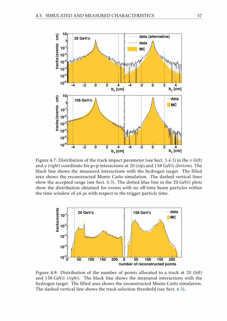
Figure 4.7 shows distribution of the impact parameter, as defined in Sect. 3.4.3.Small differences between the data and MC reveal limited accuracy of the detectorsimulation. The largest discrepancy visible for by at 20 GeV/c originates from inter-actions of beam particles close in time to the trigger particle (see Sect. 5.2.2), notsimulated in MC. When much stricter rejection of events with such off-time beamparticles is applied, the difference decreases by factor of several.
Figure 4.8 shows distribution of number of points allocated to a track. Maximavisible in the distribution correspond to tracks measured in two sectors of VTPC-1(48 points), whole VTPC-1 (72 points), VTPC-2 and a MTPC (162 points) and bothVTPCs and a MTPC (234 points). The maxima in the data distributions are lesssharp and slightly shifted towards lower values. This suggests that the point recon-struction efficiency is somewhat overestimated in simulation.
The differences between data and simulation visible in Figs. 4.6–4.8 occurmostly at the tails of the distributions. Their overall contribution to the total statis-tics is small. Systematic bias due to limited precision of the simulation was esti-mated by varying the selection cuts and was found to be below 2% (see Sect. 6.5.2).It was always significantly smaller than the other sources of the systematic uncer-tainties.
4.5. SIMULATED AND MEASURED CHARACTERISTICS 37
[cm]xb-4 -2 0 2 4
cm
)⋅
tra
ck
s/(
ev
en
ts
-610
-510
-410
-310
-210
-110
1
1020 GeV/c
[cm]yb-4 -2 0 2 4
-6
-5
-4
-3
-2
-1
1
10data (alternative)
data
MC
[cm]xb-4 -2 0 2 4
cm
)⋅
tra
ck
s/(
ev
en
ts
-610
-510
-410
-310
-210
-110
1
10158 GeV/c
[cm]yb-4 -2 0 2 4
-6
-5
-4
-3
-2
-1
1
10data
MC
Figure 4.7: Distribution of the track impact parameter (see Sect. 3.4.3) in the x (left)and y (right) coordinate for p+p interactions at 20 (top) and 158 GeV/c (bottom). Theblack line shows the measured interactions with the hydrogen target. The filledarea shows the reconstructed Monte Carlo simulation. The dashed vertical linesshow the accepted range (see Sect. 6.3). The dotted blue line in the 20 GeV/c plotsshow the distribution obtained for events with no off-time beam particles withinthe time window of ±6 µs with respect to the trigger particle time.
0 50 100 150 200
0.05
0.1
0.15
0.2
0.25
0.3
0.35
0.4
0.45
0.5
0 50 100 150 200
tra
ck
s/e
ve
nts
-510
-410
-310
-210
-11020 GeV/c
0 50 100 150 200-5
-4
-3
-2
-1data
MC
158 GeV/c
0
number of reconstructed points
Figure 4.8: Distribution of the number of points allocated to a track at 20 (left)and 158 GeV/c (right). The black line shows the measured interactions with thehydrogen target. The filled area shows the reconstructed Monte Carlo simulation.The dashed vertical line shows the track selection threshold (see Sect. 6.3).

Chapter 5
Characteristics of the dataset
5.1 Data acquired and used in the analysis
The data on proton-proton interactions were collected at five momenta of the beamparticles: pbeam = 20, 31, 40, 80 and 158 GeV/c with the NA61/SHINE detectorin 2009. The data taking periods and numbers of events collected are listed inTable 5.1. About one week was devoted for each beam momentum. The data col-lection rate was lower at the lowest beam momenta due to the secondary beamproperties (see Sect. 5.2). As a result the statistics available at 20 GeV/c is 2–3 timessmaller than at the other beam momenta.
The analysis was based on the 12D002 (40 GeV/c) and 12E002 (other reactions)reconstructions. These two reconstructions are related to different software ver-sions used for processing. The differences are irrelevant for the analysis presentedin this thesis.
The data was collected within so-called runs. A run lasts from several minutes(if the data acquisition system stops unexpectedly, typically due to minor hardwareor software faults) to several hours (optimally no more than two) and contains upto 100 k events.
An event corresponds to information read from all detectors synchronised bythe trigger signal. Simultaneously with the interaction trigger (see Eq. (2.2)) 10–20% of events with the unbiased beam trigger (see Eq. (2.1)) were taken for testpurposes. The runs were taken with target inserted and removed alternately, thelatter contributing by 5–10% to the total statistics.
Table 5.1: Information about the data collection times at each beam momentumand the total number of all triggers and target inserted and removed together. Thenumbers of triggers are given before and after verification described in this section.
pbeam data taking period first run last run statistics[GeV/c] all verified20 2009.09.21–2009.09.28 9265 9389 2.15 M 1.45 M31 2009.09.05–2009.09.14 8947 9135 3.55 M 3.49 M40 2009.10.12–2009.10.22 9451 9702 5.84 M 5.79 M80 2009.11.09–2009.11.16 9996 10148 4.99 M 4.34 M
158 2009.11.05–2009.11.09 9910 9989 3.98 M 3.98 M
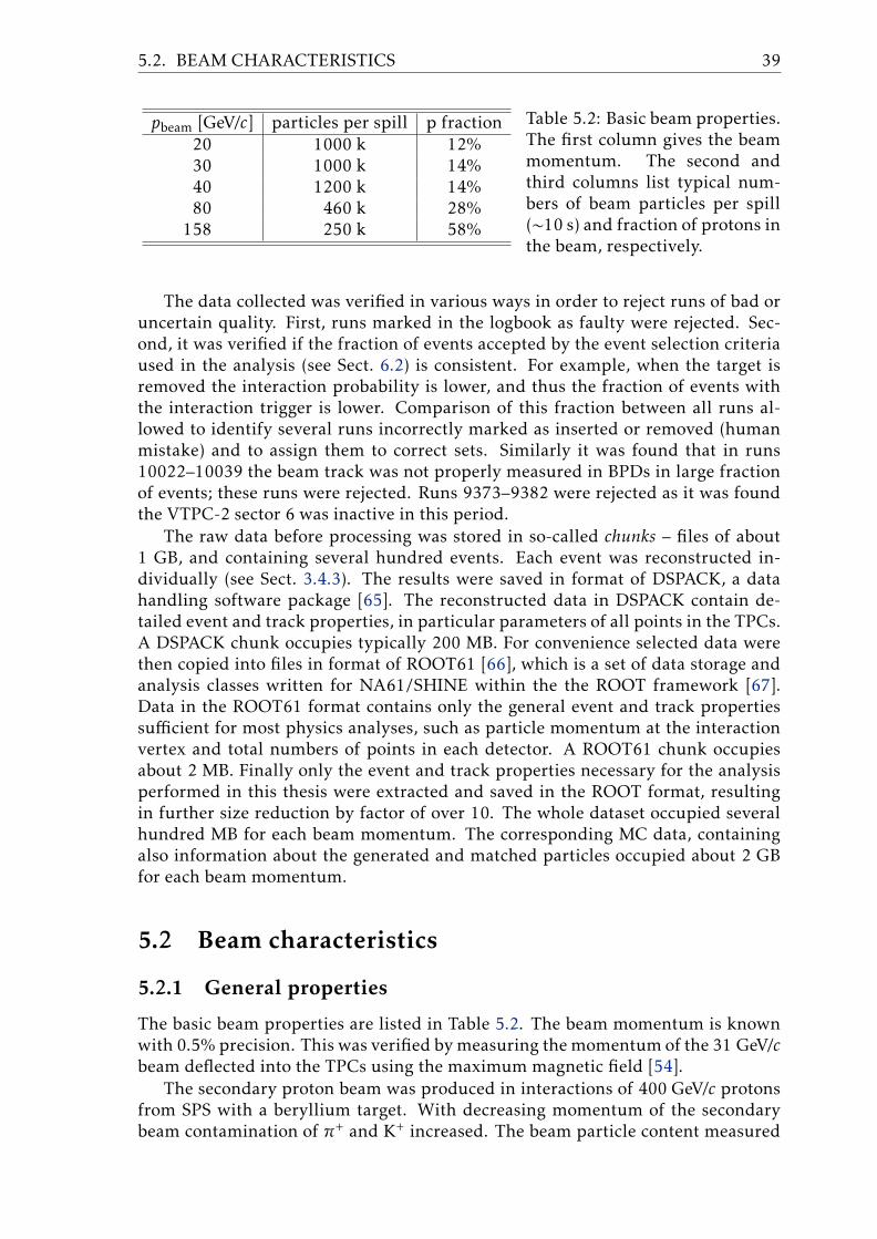
5.2. BEAM CHARACTERISTICS 39
pbeam [GeV/c] particles per spill p fraction20 1000 k 12%30 1000 k 14%40 1200 k 14%80 460 k 28%
158 250 k 58%
Table 5.2: Basic beam properties.The first column gives the beammomentum. The second andthird columns list typical num-bers of beam particles per spill(∼10 s) and fraction of protons inthe beam, respectively.
The data collected was verified in various ways in order to reject runs of bad oruncertain quality. First, runs marked in the logbook as faulty were rejected. Sec-ond, it was verified if the fraction of events accepted by the event selection criteriaused in the analysis (see Sect. 6.2) is consistent. For example, when the target isremoved the interaction probability is lower, and thus the fraction of events withthe interaction trigger is lower. Comparison of this fraction between all runs al-lowed to identify several runs incorrectly marked as inserted or removed (humanmistake) and to assign them to correct sets. Similarly it was found that in runs10022–10039 the beam track was not properly measured in BPDs in large fractionof events; these runs were rejected. Runs 9373–9382 were rejected as it was foundthe VTPC-2 sector 6 was inactive in this period.
The raw data before processing was stored in so-called chunks – files of about1 GB, and containing several hundred events. Each event was reconstructed in-dividually (see Sect. 3.4.3). The results were saved in format of DSPACK, a datahandling software package [65]. The reconstructed data in DSPACK contain de-tailed event and track properties, in particular parameters of all points in the TPCs.A DSPACK chunk occupies typically 200 MB. For convenience selected data werethen copied into files in format of ROOT61 [66], which is a set of data storage andanalysis classes written for NA61/SHINE within the the ROOT framework [67].Data in the ROOT61 format contains only the general event and track propertiessufficient for most physics analyses, such as particle momentum at the interactionvertex and total numbers of points in each detector. A ROOT61 chunk occupiesabout 2 MB. Finally only the event and track properties necessary for the analysisperformed in this thesis were extracted and saved in the ROOT format, resultingin further size reduction by factor of over 10. The whole dataset occupied severalhundred MB for each beam momentum. The corresponding MC data, containingalso information about the generated and matched particles occupied about 2 GBfor each beam momentum.
5.2 Beam characteristics
5.2.1 General properties
The basic beam properties are listed in Table 5.2. The beam momentum is knownwith 0.5% precision. This was verified bymeasuring themomentum of the 31 GeV/cbeam deflected into the TPCs using the maximum magnetic field [54].
The secondary proton beam was produced in interactions of 400 GeV/c protonsfrom SPS with a beryllium target. With decreasing momentum of the secondarybeam contamination of π+ and K+ increased. The beam particle content measured

40 CHAPTER 5. CHARACTERISTICS OF THE DATASET
Figure 5.1: Fraction of hadrons of various species per incident beam particle fromthe CEDAR counter as a function of the gas pressure within the pressure rangewhich covers maxima of π+, K+ and p at 31 (left) and 158 GeV/c (right). Figurestaken from Ref. [32].
with CEDAR is shown in Fig. 5.1. In order to retain sufficient proton rate the lowmomenta beam intensities were increased by opening the collimators. As a resultthe beam width and divergence increased, leading to higher fraction of events re-jected in the analysis. Also as the total beam intensity increased, more so-calledoff-time beam particles were arriving within the ±25 µs signal collection period ofthe TPCs. Some (about 2%) of these particles interacted and generated TPC tracksmistakenly fitted to the main vertex.
5.2.2 Off-time beam particles
Information of charged beam particles registered in the S1 counter within ±25 µswith respect to the trigger particle is saved in the event. The particle arrival timesare measured with precision of 0.1 µs, with 0.2 µs two-particle resolution. The timedistribution of the beam particles is shown in Fig. 5.2. Besides the trigger particle,large number of the off-time particles is present, in particular at the lowest beammomentum. Ratio of numbers of the on-time to off-time particles decreases byfactor of 4 from 158 to 20 GeV/c.
Figure 5.3 shows the average number of the off-time beam particles per event.At 20–40 GeV/c there is in average one off-time beam particle in the ±5 µs range. Asit will be shown the off-time beam particles within this range affect the results.
Due to electron drift in the TPCs tracks from the off-time interactions are ver-tically shifted with respect to the tracks originating from interaction of the triggerparticle. This allows to distinguish them, however some them can be incorrectlyfitted to the main vertex. This happens most often for the electrons, as they orig-inate mostly from the secondary vertices. The largest effect is visible at the lowazimuthal angles θ and particle momenta of several GeV/c.
Figure 5.4 shows the dE/dx distributions selected with two different off-timeparticle rejection criteria. When the off-time particles are rejected more strictly(right panel, with respect to the left one) the electron yield decreases, while yield ofthe negatively charged hadrons (h−) remains constant. Figure 5.5 (left) shows theelectron yield dependence on the off-time beam particles rejection range. At 20–

5.2. BEAM CHARACTERISTICS 41
s]µt [∆-25 -20 -15 -10 -5 0 5 10 15 20 25
en
trie
s
310
410
510
610
20 GeV/c
s]µt [∆-25 -20 -15 -10 -5 0 5 10 15 20 25
en
trie
s
310
410
510
610
158 GeV/c
Figure 5.2: Time distribution of the beam particles measured in the S1 counter withrespect to the trigger particle for 20 (left) and 158 GeV/c (right). The peak at ∆t = 0corresponds to the trigger particle. The rest of the distribution corresponds to theoff-time beam particles. The minimum at −2 < ∆t < 0 µs is a result of the hardwaremechanism disabling the trigger for 2 µs after each non-interacting beam particle.The other small maxima (e.g. at ∆t = ±23 µs) are related to the beam time structurein the SPS. The dashed vertical lines show the off-time particle cut window (seeSect. 6.2).
[GeV/c]beam
p20 30 40 50 100 200
# o
ff-t
ime
be
am
pa
rtic
les
0
1
2
3
4
5
6
7
8sµ25±
sµ5±
sµ2±
Figure 5.3: The average number of theoff-time beam particles per event within±2, ±5 and ±25 µs around the triggerparticle, at five beam momenta.
40 GeV/c there is a systematic effect visible up to 5 µs, no effect at 80 and 158 GeV/c.This shows that the electron tracks are fitted more poorly and electrons originatingfrom the off-time interactions are more likely to be fitted to the main vertex.
Rejecting all events with off-time beam particles within ±5 µs would imply dis-carding significant fraction of the statistics at the low beam momenta, as demon-strated in Fig. 5.5 (right). Instead, only events with off-time beam particles within±2 µs window are rejected, which corresponds to ±2.8 cm vertical shift of the VTPCtracks. Hadrons originating from the accepted off-time interaction are rejected bythe ±2 cm impact parameter cut. Electrons are rejected using dE/dx measurement(see Sect. 6.3.5).

42 CHAPTER 5. CHARACTERISTICS OF THE DATASET
p [GeV/c]
0 2 4 6
dE
/dx
[M
IP]
0.8
1
1.2
1.4
1.6
1.8
2
2.2
no
rma
lis
ed
en
trie
s
0
0.2
0.4
0.6
0.8
1
1.2
1.431 GeV/c
< 20 mradθ
no off-time cut-e
-h
p [GeV/c]
0 2 4 6
dE
/dx
[M
IP]
0.8
1
1.2
1.4
1.6
1.8
2
2.2
no
rma
lis
ed
en
trie
s
0
0.2
0.4
0.6
0.8
1
1.2
1.431 GeV/c
< 20 mradθ
sµ2 ±off-time cut -e
-h
Figure 5.4: The dE/dx distribution of the negatively charged tracks selected withthe event and track selection criteria described in Sects. 6.2 and 6.3, measured at31 GeV/c. The tracks were selected in the azimuthal angle range θ = arcsin(pT/p) <20mrad. No off-time particle rejection was used for the left panel, while only eventswith no off-time beam particles within ±2 µs are accepted in the right panel. Thenumber of entries was divided by the number of events and by the p, dE/dx andθ bin size. The upper band on the plot corresponds to electrons, and the lowerband to negatively charged hadrons (h−), mostly π−. The dashed rectangle showsthe selection range used to count electrons in Fig. 5.5 (left).
s]µ[±off-time cut window
0 1 2 3 4 5 6 7 8 9 10
]-1
rad
)⋅
[(G
eV
/cθ
dp
dd
n
0
0.01
0.02
0.03
0.04
0.05
0.06
0.07
0.08electrons
< 20 mradθ
2 < p < 4 GeV/c
s]µ[±off-time cut window
0 2 4 6 8 10
nu
mb
er
of
ev
en
ts
510
610
158 GeV/c
80 GeV/c
40 GeV/c
31 GeV/c
20 GeV/c
Figure 5.5: Left: The electron yield for θ < 20 mrad and 2 < p < 4 GeV/c at five beammomenta, for events selected with no off-time beam particle closer to the triggerparticle than the time given on abscissa (0 µs corresponds to no event rejection).Electrons were identified using dE/dx measurement, as shown in Fig. 5.4. Right:Number of events as a function of the off-time beam particles rejection range.

5.2. BEAM CHARACTERISTICS 43
Requirement of good quality of signal measured in the BPDs provide additionalrejection of events with an off-time particle arriving within ±100 ns. As the BPDintegration time equals approximately 300 ns, two particles would induce a doublepeak signal which cannot be reconstructed properly.
Any remaining effects related to the off-time beam particles are included in thesystematic uncertainty (see Sect. 6.5.2).
5.2.3 Beam profile and divergence
The beam profiles measured in BPD-3 are shown in Fig. 5.6 (top). The beam widthis much wider at the lowest momentum. The shape of the V1 counter is clearlyvisible, suggesting that the actual beamwidth is even larger than the accepted beamfraction.
Figure 5.6 (bottom) shows distribution of the beam angle with respect to thenominal beam axis measured in BPDs. The beam divergence is narrower at thehigh momenta. However, as it will be shown in Sect. 6.3.4 the particle momentaare more affected by the beam angle variation at the high beam momenta, as theeffect concerns only the high momentum produced particles.
x [cm]-0.5 0 0.5
y [
cm
]
-0.8
-0.6
-0.4
-0.2
0
0.2
0.4
0.6
0.8 20 GeV/c
= 0.55 cmyFWHM
= 0.55 cmxFWHM
x [cm]-0.5 0 0.5
-0.8
-0.6
-0.4
-0.2
0
0.2
0.4
0.6
0.8
en
trie
s [
arb
. u
nit
s]
0
1
2
3
4
5
6
7
8
9
10
158 GeV/c
= 0.25 cmyFWHM
= 0.25 cmxFWHM
div x [mrad]-1 0 1
div
y [
mra
d]
-1.5
-1
-0.5
0
0.5
1
1.5 20 GeV/c
= 0.90 mradyFWHM
= 0.80 mradxFWHM
div x [mrad]-1 0 1
-1.5
-1
-0.5
0
0.5
1
1.5
en
trie
s [
arb
. u
nit
s]
0
1
2
3
4
5
6
7
8
9
10
= 0.10 mradyFWHM
= 0.20 mradxFWHM
158 GeV/c
Figure 5.6: Top: The beam spot as measured by BPD-3 for 20 (left) and 158 GeV/c(right) beammomenta. The circular outline of the distribution corresponds to shapeof the hole in the V1 counter. Bottom: The beam divergence in x and y for 20 (left)and 158 GeV/c (right) beam momenta. All distributions were arbitrarily scaled tothe full colour scale. Widths of the distributions are given in the legend.

44 CHAPTER 5. CHARACTERISTICS OF THE DATASET
vertex z [cm]
-600 -590 -580 -570 -560
en
trie
s
1
10
210
310
410
51031 GeV/c inserted
removed
vertex z [cm]
-600 -590 -580 -570 -560
en
trie
s
1
10
210
310
410
510158 GeV/c inserted
removed
Figure 5.7: Distributions of the fitted vertex z coordinate for the target insertedand removed in events taken with an unbiased beam trigger at 31 GeV/c (left) and158 GeV/c (right). For the best resolution, only events with at least 7 tracks wereselected. The target removed distribution was normalised to the vertex distributionfar away from the target cell, as described in Sect. 6.4.1. The vertical dashed linesshow the z range used to calculate the interaction rates shown in Fig. 5.8.
[GeV/c]beam
p20 30 40 50 100 200
in
tera
cti
on
ra
te [
%]
targ
et
ins
ert
ed
targ
et
rem
ov
ed
0
0.1
0.2
0.3
0.4
0.5
0.6
0.7
0.8
0.9
1
Figure 5.8: Ratio of interaction rateswith hydrogen in the target cell in tar-get removed (gaseous hydrogen residue)and inserted. It is calculated as a ratio ofthe number of entries with the vertex fit-ted within ±1 cm around the target cen-tre (z = −581 cm) for target removed nor-malised, and target inserted, as shownin Fig. 5.7. Events with at least 7 trackswere selected. The analysis was not per-formed for 20 GeV/c due to insufficientdata statistics.
5.3 Target density
An analysis described in Ref. [68] showed discrepancy of up to 7% at 80 GeV/cbetween the p+p interaction cross-section measured by NA61/SHINE and the lit-erature values. A possible explanation was variation of the target density ratiobetween target inserted and removed, possibly due to boiling of the liquid hydro-gen. Uncertainty of knowledge of this ratio affects the cross-section uncertaintyproportionally.
The density ratio of the target removed and inserted was calculated from therelative interaction rates in the unbiased beam trigger data (see Eq. (2.1)). Figure 5.7shows the fitted vertex z distributions for target removed and inserted. Only thehigh multiplicity events were selected to ensure good fit resolution. The maxima

5.4. RECONSTRUCTION EFFICIENCY AND RESOLUTION 45
at z = −591 cm and z = −571 cm in the target removed distributions correspond tointeractions with the target cell windows. Entries between the maxima correspondto interactions with the gaseous hydrogen residue. The numbers of events in thisregion for target removed (normalised) and inserted were divided to calculate therelative interaction rate with gaseous hydrogen, shown in Fig. 5.8 for various beammomenta. The ratio varies from 0.2% to 0.5%, which corresponds to about ±50%relative variation. This result agrees with the hypothesis that the difficulties tocalculate the cross-section are related to variable target removed to inserted densityratio in various datasets. The other likely explanations of these difficulties wereruled out [68].
The ±50% uncertainty or variability of the target density significantly limitsprecision of determination of inelastic cross-section. The pion spectra presented inthis thesis are determined from particle yields per selected event and thus they areindependent of the target density.
5.4 Reconstruction efficiency and resolution
Properties of reconstruction were studied using MC. The simulated and recon-structed information of the matched tracks were compared.
The reconstruction efficiency was calculated by checking what fraction of thesimulated π− is reconstructed and passes the selection criteria. In order to limitimpact of the possible imperfect implementation of the detector shape in simula-tion, only the regions with good reconstruction efficiency (>90%) are selected forthe analysis (see Sect. 6.3.3). The reconstruction efficiency in these regions calcu-lated using MC is close to 100%, as demonstrated in Fig. 5.9.
y0 1 2 3 4
[G
eV
/c]
Tp
0
0.5
1
1.5
97 98 98 97 97 98 98 96
98 98 98 98 98 99 99 99
99 99 99 98 99 99 98
99 99 99 99 99 99
99 99 99 99 99
99 99 99 99 98
99 99 99 99
99 99 99 99
99 100
20 GeV/c
eff
icie
nc
y [
%]
95
96
97
98
99
100
y0 1 2 3 4
0
0.5
1
1.5
100 100 97 98 99 98 98 98 97
100 99 98 99 99 99 99 98
100 100 99 99 99 99 99 99 96
100 99 99 99 99 99 99 99
100 99 99 99 99 99 99 98
99 99 99 99 99 99
99 99 99 99 99 99
99 99 99 99 99 97
99 99 99 100 98
158 GeV/c
0
Figure 5.9: Reconstruction efficiency of negatively charged pions produced in p+pinteractions simulated in EPOS at 20 (left) and 158 GeV/c (right) as a function ofrapidity and the transverse momentum. It was calculated by dividing the numberof tracks passing the track selection cuts specified in Sect. 6.3 by the number of thegenerated tracks. The selection criteria include selection of the azimuthal angle φregions with at least 90% reconstruction efficiency. Only tracks with at least 25 gen-erated points were used. For clarity, the numbers printed are averages calculatedin four adjacent bins.

46 CHAPTER 5. CHARACTERISTICS OF THE DATASET
[GeV/c]T
- MC pT
Matched p-0.1 -0.05 0 0.05 0.1
en
trie
s
1000
2000
3000
4000
5000
6000
158 GeV/c<0.15 GeV/c
T0.0<y<0.2, 0.10<p
RMS = 0.0088 GeV/c = 0.0023 GeV/c(68%)quantile = 0.0137 GeV/c(95%)quantile = 0.0020 GeV/c
fitσ
= 0.0030 GeV/cFWHM
[GeV/c]T
- MC pT
Matched p-0.1 -0.05 0 0.05 0.1
en
trie
s
50
100
150
200
250
158 GeV/c<0.50 GeV/c
T1.8<y<2.0, 0.45<p
RMS = 0.0142 GeV/c = 0.0100 GeV/c(68%)quantile = 0.0195 GeV/c(95%)quantile = 0.0093 GeV/c
fitσ
= 0.0210 GeV/cFWHM
Figure 5.10: Distributions of differences between the generated and reconstructedtransverse momentum of matched MC tracks in selected (y, pT) bins. Results ofseveral methods to estimate width of the peak are given in the legend (see text forexplanation). The dark red, orange, green and aquamarine points distinguish quan-tiles covering 68%, 95%, 99.7% and 99.99% statistics in the middle, respectively.The horizontal blue line shows the full width at half maximum (FWHM).
0 1 2 3 4
[G
eV
/c]
Tp
0
0.5
1
1.5
16 16 14 15 16 17 1314 13 13 12 15 18 15 8
8 11 9 10 12 22 20
6 10 8 8 11 285 8 8 7 7 17
5 7 6 6 8
5 6 6 5 7
4 5 5 4
4 4
20 GeV/c
y0 1 2 3 4
[G
eV
/c]
Tp
0
0.5
1
1.5
3 4 3 4 4 6 5
5 5 5 5 6 8 7 4
10 10 7 7 8 18 1314 14 11 9 10 24
23 19 13 11 15 26
30 26 20 16 10
40 30 20 16 19
58 39 29 16
54 24
20 GeV/c
310
×(y
reso
luti
on
)
0
5
10
15
20
25
30
35
40
45
50
0 1 2 3 40
0.5
1
1.5
8 8 9 10 10 14 16 18 1612 12 13 13 14 24 28 28 24
12 13 12 12 20 36 33 3512 13 11 12 28 36 33 3610 10 9 12 34 33 44
10 8 9 16 33 30 31
9 8 8 21 33 35
8 6 6 24 30 41
6 5 6 26 30
158 GeV/c
re
so
luti
on
[M
eV
/c]
Tp
0
5
10
15
20
25
30
35
40
45
50
y0 1 2 3 4
0
0.5
1
1.5
2 3 3 3 3 5 7 6 6
3 3 4 3 4 7 9 8 64 4 4 4 6 12 11 14
5 5 4 5 11 15 13 127 6 5 7 19 18 23
8 6 6 11 22 20 21
10 8 7 18 26 32
12 8 8 26 34 47
16 10 10 38 57
158 GeV/c
0
0 0
Figure 5.11: Resolution of rapidity (top, multiplied by 103) and the transverse mo-mentum (bottom) measurements for negatively charged pions produced in p+p in-teractions at 20 (left) and 158 GeV/c (right) as a function of pion rapidity and thetransverse momentum. The results are obtained using the track selection cuts spec-ified in Sect. 6.3. For clarity, the numbers printed are averages calculated in fouradjacent bins.

5.4. RECONSTRUCTION EFFICIENCY AND RESOLUTION 47
Resolution of rapidity and the transverse momentum was calculated as a widthof the distribution of differences between y and pT of the generated π− particles andcorresponding matched tracks. Figure 5.10 shows example distributions derived inselected (y, pT) bins. Several methods to estimate width of the distribution wereexamined.
• Simple calculation of RMS often overestimated the value due to long tails ofthe distribution.
• The distribution were divided into quantiles covering to 68%, 95%, 99.7% and99.99% statistics in the middle of the distribution, which would correspondto 1σ , 2σ , 3σ and 4σ respectively in case of Gaussian distribution. The leftpanel shows that the 95% quantile is often much more than twice wider thanthe 68% one.
• Gaussian distribution was fitted in region from −2RMS to +2RMS, and itswidth σ was taken as a width estimate.
• FWHM of the distribution was calculated. In the lowest statistics (y, pT) binsthe histogram bin widths were increased until FWHM could be calculatedunambiguously.
Out of the method described above FWHM was chosen, as it was not sensitive tolong tails of the distributions and yielded the most reasonable results in both lowand high statistics bins. Resulting resolution of rapidity and the transverse mo-mentum reconstruction is shown in Fig. 5.11.
Due to limited reconstruction resolution the reconstructed tracks can be as-signed to incorrect (y, pT) bin. This effect is called bin migration. In order to min-imise this effect, the bin sizes were chosen larger than the reconstruction resolution.
Figure 5.12 shows distributions of the invariant mass of secondary π+π− pairsin the measured data and in simulation. The difference between the peak positionand the literature value of K0
S mass is below 1 MeV/c2. This demonstrates resolutionof the momentum reconstruction, and correctness of the magnetic field calibration.The width of the MC distribution is about 25% smaller than for the data. This im-plies that statistical or systematic uncertainties of track parameters reconstructedfrom the data are slightly underestimated in the simulation. As it will be demon-strated in Sect. 6.5.2 these imperfections have low impact on the final results.

48 CHAPTER 5. CHARACTERISTICS OF THE DATASET
0.45 0.5 0.55
co
un
ts
0
5
10
15
20
25
30
35
40
45 data
MC
20 GeV/c
]2) [GeV/c-π+π(inv
m
0.45 0.5 0.55
co
un
ts
0
500
1000
1500
2000
2500158 GeV/c
0
Figure 5.12: Invariant mass distributionof reconstructed π+π− pairs in p+p in-teractions at 20 (top) and 158 GeV/c (bot-tom) for the measured data and EPOSmodel based Monte Carlo simulations.The peak at m ≈ 0.5 GeV/c correspondsto K0
S decays. The MC plot was nor-malised to the peak height of the datadistribution. The K0
S candidates wereselected within 0< y < 1 and 0<pT <0.5 GeV/c for 20 GeV/c and −1< y < 0 and0<pT < 0.5 GeV/c for 158 GeV/c. In or-der to reduce background, the secondaryvertices were selected at cτ > 1.0 cm fory < 0.5 and cτ > 1.5 cm for y > 0.5. Thedata distribution was fitted with a sumof a Lorentzian function (signal) and asecond order polynomial (background).Figure taken from Ref. [29].

Chapter 6
Data analysis
6.1 Overview of the analysis procedure
Spectra of the π− mesons produced in p+p collisions at the beam momenta of 20,31, 40, 80, and 158 GeV/c were obtained with so-called h− method. The analysis isbased on the fact that the majority of produced negatively charged hadrons (h−) arepions [25–27]. The particle charge is measured and non-hadrons (i.e. electrons) arerejected based on the dE/dx measurement. Contribution of other particles (mostlyK−, p and secondary particlesmistakenly fitted to themain vertex) is removed usingthe Monte Carlo (MC) simulation. MC is also used to correct for other experimentaleffects, which will be described in this chapter.
The final results refer to the π− mesons produced in inelastic p+p interactionsby the strong interaction processes and in electromagnetic decays of produced had-rons. Such pions are referred to as primary π−. The term primarywill be used in theabove meaning also for other particles. Particles produced in weak decays or in-teractions of the produced particles are called secondary. The spectra represent theaverage number of particles produced in event in given bin of a two-dimensionalhistogram in rapidity y and the transverse momentum pT or transverse mass mT,divided by the size of the bin.
The procedure used for the data analysis consists of the following steps:
(i) applying event (Sect. 6.2) and track (Sect. 6.3) selection criteria,(ii) determination of spectra of negatively charged hadrons using the selected
events and tracks,(iii) evaluation of corrections to the spectra, based on experimental data and sim-
ulations (see Sect. 6.4),(iv) calculation of the corrected spectra,(v) calculation of the statistical and systematic uncertainties (see Sect. 6.5).
Corrections for the following data biases were evaluated and applied:
(i) geometrical acceptance and impact of the beam angle variation,(ii) contribution of off-target interactions,(iii) contribution of the negatively charged particles other than π− produced in
inelastic p+p interactions,(iv) rejection of some of the inelastic p+p interactions as well as of the π− tracks
produced in accepted interactions due to the trigger and the event and trackselection criteria employed in the analysis, as well as the track migration be-

50 CHAPTER 6. DATA ANALYSIS
y0 1 2 3 4
[G
eV
/c]
Tp
0
0.2
0.4
0.6
0.8
1
1.2
1.4
this analysis
dE/dx
ToF
20 GeV/c
y0 1 2 3 4
[G
eV
/c]
Tp
0
0.2
0.4
0.6
0.8
1
1.2
1.4 158 GeV/c
Figure 6.1: Typical acceptance regions for the π− meson spectra in p+p interac-tions at 20 GeV/c (left) and 158 GeV/c (right) for different analysis methods: themethod used in this thesis which does not require an explicit pion identification,the method which identifies pions via their energy loss (dE/dx) and time of flight(ToF) [48].
y0 1 2 3 4
[G
eV
/c]
Tp
0
0.2
0.4
0.6
0.8
1
1.2
1.4
y0 1 2 3 4
]2
[G
eV
/cT
m
0
0.2
0.4
0.6
0.8
1
1.2
1.4
Figure 6.2: The histogram bin ranges used for (y, pT) (left) and (y, mT) (right).
tween the histogram bins due to finite momentum resolution and other effectsrelated to detection and reconstruction.
These steps are described in the successive subsections.
The typical acceptance in rapidity and the transverse momentum for p+p in-teractions at 20 and 158 GeV/c is presented in Fig. 6.1. This figure also shows ac-ceptance regions for methods based on explicit pion identification using dE/dx andtime of flight measurements. They are limited due to the geometrical acceptanceof the ToF detectors, the finite resolution of the dE/dx measurements and limitedstatistics of the experimental data.
The analysis was performed in (y, pT) and (y, mT) bins. Corrections as well asstatistical and systematic uncertainties were calculated for each bin independently.

6.2. EVENT SELECTION 51
The binning scheme is shown in Fig. 6.2. The bin sizes were selected taking intoaccount the statistical uncertainties as well as the resolution of the momentum re-construction. The bins in rapidity are of constant width of 0.2. Widths of the pTbins equal 0.05 GeV/c up to pT = 0.6 GeV/c, 0.1 GeV/c for 0.6 < pT < 1 GeV/c, and0.25 GeV/c up to pT = 1.5 GeV/c.
The mT bins were selected in order to match the binning used for the Pb+Pb ex-perimental results at 20 and 30A GeV/c in Ref. [9], and extended above 0.96 GeV/c2
up to 1.4 GeV/c2. Widths of the bins equal 0.06 GeV/c2 up to mT = 0.84 GeV/c2,and the further bins end at 0.90, 0.96, 1.08, 1.20 and 1.40 GeV/c2. The spectra ob-tained in Pb+Pb collisions at 40, 80 and 158A GeV/c [8] were derived in different,0.05 GeV/c constant size mT bins, and extended only up to mT = 0.75 GeV/c2. Inorder to simplify comparison of the data it was decided to use the same binning forall beam momenta and to interpolate the Pb+Pb data at high beam momenta.
The data were analysed using ROOT and ROOT61 code dedicated for this task.
6.2 Event selection
6.2.1 List of event selection criteria
The following on-line (the interaction trigger condition) and off-line event selectioncriteria were applied to the events recorded with the interaction trigger:
(i) interaction is recognised by the trigger logic defined in Eq. (2.2),(ii) no off-time beam particle is detected within ±2 µs with respect to the trigger
particle S1 signal,(iii) The beam particle trajectory is measured in BPD-3 and at least one of BPD-1
or BPD-2.(iv) there is at least one track reconstructed in the TPCs and fitted to the interac-
tion point (see Sect. 6.2.2),(v) if the vertex is found by the reconstruction algorithms, its z position lies
within ±40 cm from the LHT centre (see Sect. 6.2.2),(vi) events with a single, positively charged primary hadron track of total momen-
tum within several GeV/c with respect to the beam momentum are rejected(see Sect. 6.2.3).
The numbers of events selected for the analysis are shown in Table 6.1. At eachbeam momentum several millions events are collected for target inserted, exceptfor 20 GeV/c due to slower data acquisition rate (see Sect. 5.2). The target removedstatistics was aimed to be 5–10% of the total statistics, as this is sufficient to achievethe necessary statistical precision for the off-target interactions. This fraction isfurther reduced by the event selection criteria described above. About 5 millions ofsimulated events were generated at each beam momentum.
In the measured data p+p interactions were selected by the trigger logic (cut (i),see Sect. 2.2). In simulation however, all inelastic events are available. In order tomimic the trigger behaviour cut (i) is reproduced by requiring lack of the S4 signal.Fraction of events lost due to use of the S4 counter is of order of 1–2% at the lowbeam momenta, but increases to 16% at 158 GeV/c. This effect is corrected usingMC (see Sect. 6.4.3).

52 CHAPTER 6. DATA ANALYSIS
Table 6.1: Numbers of events selected for analysis after consecutive selection cri-teria listed in Sect. 6.2.1, for target inserted, removed and EPOS MC. The first line(*) gives the number of events before S4 selection (cut (i)) for MC. Numbers aregiven in thousands (k = 103). The numbers in round brackets give the percentagewith respect to cut (i), and numbers in the square brackets give the percentage withrespect to the previous cut.
cut target inserted target removed EPOSpbeam = 20 GeV/c
(*) – – – – – – 4 975k (100.7) –(i) 1 257 k (100.0) – 109.2 k (100.0) – 4 939k (100.0) [99.3](ii) 790 k (62.8) [62.8] 69.1 k (63.3) [63.3] – – –(iii) 477 k (37.9) [60.4] 25.1 k (23.0) [36.4] – – –(iv) 276 k (22.0) [57.9] 7.0 k (6.4) [27.8] 4 377 k (88.6) [88.6](v) 255 k (20.3) [92.4] 3.8 k (3.5) [54.1] 4 351 k (88.1) [99.4](vi) 233 k (18.5) [91.1] 3.6 k (3.3) [93.8] 4 274 k (86.5) [98.2]
pbeam = 31 GeV/c(*) – – – – – – 4 980k (101.5) –(i) 2 839 k (100.0) – 248.3 k (100.0) – 4 905k (100.0) [98.5](ii) 1 839 k (64.8) [64.8] 156.1 k (62.9) [62.9] – – –(iii) 1 438 k (50.7) [78.2] 83.7 k (33.7) [53.6] – – –(iv) 955 k (33.6) [66.4] 31.3 k (12.6) [37.4] 4 432 k (90.4) [90.4](v) 875 k (30.8) [91.7] 14.9 k (6.0) [47.8] 4 404 k (89.8) [99.4](vi) 843 k (29.7) [96.3] 14.6 k (5.9) [97.6] 4 372 k (89.1) [99.3]
pbeam = 40 GeV/c(*) – – – – – – 4 992k (102.4) –(i) 4 684 k (100.0) – 364.9 k (100.0) – 4 874k (100.0) [97.6](ii) 3 021 k (64.5) [64.5] 228.2 k (62.5) [62.5] – – –(iii) 2 529 k (54.0) [83.7] 150.2 k (41.2) [65.8] – – –(iv) 1 761 k (37.6) [69.6] 77.3 k (21.2) [51.5] 4 470 k (91.7) [91.7](v) 1 625 k (34.7) [92.2] 45.3 k (12.4) [58.5] 4 439 k (91.1) [99.3](vi) 1 578 k (33.7) [97.1] 44.3 k (12.1) [97.9] 4 404 k (90.4) [99.2]
pbeam = 80 GeV/c(*) – – – – – – 4 990k (107.7) –(i) 3 387 k (100.0) – 234.1 k (100.0) – 4 632k (100.0) [92.8](ii) 2 955 k (87.2) [87.2] 202.5 k (86.5) [86.5] – – –(iii) 2 133 k (63.0) [72.2] 128.9 k (55.1) [63.7] – – –(iv) 1 675 k (49.5) [78.5] 86.7 k (37.0) [67.2] 4 373 k (94.4) [94.4](v) 1 546 k (45.7) [92.3] 54.5 k (23.3) [62.9] 4 337 k (93.6) [99.2](vi) 1 543 k (45.6) [99.8] 54.4 k (23.3) [99.8] 4 332 k (93.5) [99.9]
pbeam = 158 GeV/c(*) – – – – – – 4 984k (118.9) –(i) 2 828 k (100.0) – 159.9 k (100.0) – 4 193k (100.0) [84.1](ii) 2 634 k (93.2) [93.2] 148.8 k (93.1) [93.1] – – –(iii) 1 981 k (70.1) [75.2] 103.5 k (64.7) [69.6] – – –(iv) 1 783 k (63.1) [90.0] 80.5 k (50.3) [77.8] 4 055 k (96.7) [96.7](v) 1 650 k (58.4) [92.5] 51.1 k (32.0) [63.5] 4 008 k (95.6) [98.8](vi) 1 650 k (58.4) [100.0] 51.1 k (32.0) [100.0] 4 008 k (95.6) [100.0]

6.2. EVENT SELECTION 53
Non-biasing cuts (ii) and (iii) reduce number of tracks from the off-time in-teractions and ensure good resolution of the interaction point position. Only 7%of events is removed by the off-time particle rejection (cut (ii)) at 158 GeV/c, butthis fraction increases to almost 40% at 20 GeV/c due to higher beam intensity (seeSect. 5.2.2). Another 25–40% of events is removed by cut (iii). This is related tointeractions between BPD-1 and BPD-3 and to the off-time beam particles closerthan 100 µs to the beam particle.
Cuts (iv) and (vi) remove the elastic interactions. As it is estimated with thesimulation, cut (iv) removes from 3% events at 158 GeV/c to 11% at 20 GeV/c of in-elastic interactions. As the produced particle multiplicity is lower at the low beammomenta, the vertex point is less likely to be found. The elastic event rejection willbe discussed in detail in Sect. 6.2.2.
Cut (v) is supposed to remove interactions outside the hydrogen in the targetcell. The cut removes about 40% of events with the target removed. The remain-ing 60% correspond mostly to interactions with the target cell windows. The cutremoves about 8% of the events with the target inserted (containing only smallfraction of off-target interactions) and only 1% of the simulated events (containingexclusively interactions with the target). The off-target interaction rejection will bediscussed in detail in Sect. 6.2.3.
The corrections for the remaining accepted contribution of interactions outsidethe hydrogen in the target cell and for the loss of inelastic events due to finite vertexposition reconstruction are presented in Sects. 6.4.1 and 6.4.3.
6.2.2 Elastic event rejection
In case of an elastic interaction the beam proton might get deflected far enoughto miss the S4 counter of 1 cm diameter, located at z = −212 cm, which is 359 cmfrom the target downstream window. The trigger logic accepts such events as in-teractions. The goal of the experiment is to measure characteristics of the inelasticinteractions, therefore one needs to correct for contribution of the elastic interac-tions accepted by the trigger.
The possible strategy is to accept all events in the analysis, and correct the re-sulting cross-sections using MC. However, due to uncertainty of the cross-sectionmeasurement in the p+p data (see Sect. 5.3) this approach could not be used.
Instead, two cuts were used to reject the elastic events:
• Requirement of tracks in the TPCs (cut (iv)). In an elastic interaction noparticles are produced and at most one track of the deflected beam protonis expected to be measured in the TPCs. With high probability the vertexpoint is not found, since the track may pass through the gap between theleft and right sides of the TPCs undetected (GAP TPC alone does not allowto reconstruct a track). Part of the elastic events can be thus removed byrequiring a successful vertex fit.It was however observed that for the lowmultiplicity events the vertex fit fails2% more likely in the measured data than in the simulated. This is probablycaused by slight overestimation of the reconstruction efficiency in simulation.Strict vertex fit requirement would bias the results in a way that could notbe corrected with MC. Instead, events with an unsuccessful vertex fit are re-

54 CHAPTER 6. DATA ANALYSIS
p [GeV/c]16 18 20 22 24
tra
ck
s/e
ve
nts
0
0.002
0.004
0.006
0.00820 GeV/c
p [GeV/c]35 40 45
0
0.002
0.004
0.006
0.00840 GeV/c
p [GeV/c]100 120 140 160
0
0.002
0.004
0.006
0.008158 GeV/c
Figure 6.3: Themomentum distributions of the positively charged particles for dataobtained at 20 (left), 40 (middle) and 158 GeV/c (right) beam momenta. Only eventspassing the event cuts (ii)–(v) and containing a single track are accepted. The tracksare required to pass the selection cuts and to have at least 3 points measured in theGAP TPC. The maxima visible in the 20 and 40 GeV/c panels originate from elasticscattering of the beam particle. The vertical dashed lines show the threshold levelsused to reject the elastic interactions, also listed in Table 6.2
pbeam [GeV/c] pmin [GeV/c]20 1731 2840 3580 74158 –
Table 6.2: Momentum thresholds pmin used toreject elastic interactions at each beam momen-tum, derived from the momentum distributionsshown in Fig. 6.3. The threshold is not derived at158 GeV/c where the elastically deflected beam re-mains outside of the TPC acceptance.
moved, only if they also contain no other hadron tracks in the TPCs (e± aredistinguished with dE/dx (data) and matching (MC, see Sect. 4.3)).
• Rejection of events with a single positively charged primary trackwithmo-mentum close to the beam momentum (cut (vi)). Figure 6.3 demonstratesthat in the events passing cut (v) the total momentum distribution showsa maximum slightly below the beam momentum value. It is attributed toelastically deflected beam particles measured in the GAP TPC, MTPC-L andsometimes VTPC-2. Another cut is required to remove such events.An event is classified as an elastic interaction and thus rejected if it containsa single, positively charged primary hadron track passing track cuts with atleast 3 points in the GAP TPC, and exceeding threshold momentum. Thethresholds listed in Table 6.2 were derived from the momentum distributionsexemplified in Fig. 6.3. As shown in the figure, at the beam momentum of158 GeV/c almost no particles above 120 GeV/c are measured. For this reasonthe cut is not used at 158 GeV/c.
The two cuts described above remove some class of the inelastic interactions.This effect is corrected by applying the same cuts in the simulation used to derivethe correction for event losses described in Sect. 6.4.3.

6.3. TRACK SELECTION 55
fitted vertex z [cm]700− 600− 500− 400− 300−
]-1
ev
en
ts/d
z [
cm
210
310
410
510
normalization region
target inserted
3.69)×target removed (
Figure 6.4: Distribution of fitted vertex z coordinate for target inserted and re-moved at 40 GeV/c. The distribution for the data recorded with the removed liquidhydrogen was multiplied by a factor equal to the ratio of events at z > −450 cm(region marked with a vertical arrow). The short-dashed vertical lines mark theselected z region.
The precision of the correction depends on the event generator. It is assumedthat the fraction of events removed by the cut and their properties do not differmuch in the simulation.
6.2.3 Off-target interaction rejection
In order to remove interactions occurring out of hydrogen target, events with thevertex fitted outside of the target were rejected (cut (v)). Example distributions ofthe fitted vertex z coordinate for target inserted and removed are shown in Fig. 6.4.The distributions are broadened due to limited reconstruction resolution. However,at the distances larger than 1 m from the target cell both distributions have thesame shape, as the reconstructed vertices originate from interactions with the de-tector material only. It was therefore decided to remove the events with the vertexz position located outside of the z ∈ [−620, −540] cm range, also marked in Fig. 6.4.The same cut was applied in the analysis of simulated events in order to correct forpotential biases introduced by this cut. As stated in the previous subsection, eventswith the unsuccessful vertex fit are included in the analysis.
6.3 Track selection
6.3.1 List of track selection criteria
In order to select correctly reconstructed tracks of primary negatively charged had-rons as well as to reduce the contamination of tracks from secondary interactions,weak decays and off-time interactions the following track selection criteria wereapplied:

56 CHAPTER 6. DATA ANALYSIS
(i) the track is fitted to the main interaction vertex,(ii) the track curvature corresponds to a negatively charged particle,(iii) the fitted trackmomentum component px is negative (so-called right side track,
see Sect. 6.3.2 for explanation),(iv) the track is measured in a high (≥90%) reconstruction efficiency region of
TPCs, which is defined Sect. 6.3.3,(v) the total number of reconstructed points on the track is greater than 30,(vi) the sum of the number of reconstructed points in VTPC-1 and VTPC-2 is
greater than 15 or the number of reconstructed points in the GAP TPC isgreater than 4,
(vii) the impact parameter (defined in Sect. 3.4.3) does not exceed 4 cm in thehorizontal (bending) coordinate and 2 cm in the vertical (drift) coordinate,
(viii) tracks classified as electrons of momenta below 20 GeV/c are rejected (seeSect. 6.3.5).
Cuts (i), (v) and (vi) ensure the track was well measured and the momentum res-olution is good, as shown in Sect. 5.4. In particular tracks with points in the GAPTPC only are rejected. Cuts (iii) and (iv) reduce the systematic biases related to thenon-uniform detection efficiency whichmight be simulated inaccurately. Addition-ally cut (vii) helps to reject tracks which do not originate from the main vertex. Itwas found out that these three cuts are partially redundant [69]. Cuts (ii) and (viii)are necessary to select negatively charged hadrons.
Table 6.3 gives the numbers of tracks after consecutive cuts. The number oftracks decreases with decreasing momentum of the beam particles. This is dueto lower particle multiplicity at lower collision energies and lower detector accep-tance despite of the magnetic field adjustment. Additionally at pbeam = 20 GeV/cthe number of events collected was 2–3 times smaller than for other datasets.
Negative charge selection (cut (ii)) removes more than half of the tracks: about70% at 20 GeV/c and about 60% at 158 GeV/c. This is a result of the electric chargeconservation in the two proton system. The average number of the negativelycharged produced particles increases from 〈n−〉 ≃ 1 at 20 GeV/c to 〈n−〉 ≃ 2.5 at158 GeV/c [63], while the number of the positively charged particles 〈n+〉 = 〈n−〉+2(where 2 is charge of two interacting protons).
Tracks with px > 0 removed by cut (iii) constitute about 51% of all tracks at158 GeV/c, but this fraction decreases to about 45% at the lower beam momenta,due to different detector acceptance for wrong and right side tracks for differentcollision energies and magnetic field configurations.
The acceptance cut (iv) removes 30% tracks at 20 GeV/c and only 5% at158 GeV/c.
Each of the cuts (v)–(vii) ensuring good reconstruction properties removes sev-eral percent tracks. Distributions of the impact parameter and number of points inthe data and in MC generated tracks are shown in Figs. 4.7 and 4.8. The track loss isslightly higher for the target removed, as the tracks produced outside of the targetregion have worse reconstruction properties. The loss for MC is smaller which canbe attributed to slight overestimation of detection efficiency in the simulation, butalso the lack of the off-time beam particles and off-target interactions. The frac-tion of tracks removed is larger at the low beam momenta due to slightly worsereconstruction efficiency.

6.3. TRACK SELECTION 57
Table 6.3: Numbers of tracks in events selected for analysis after consecutive selec-tion criteria listed in Sect. 6.3.1, for target inserted, removed and EPOS MC. Onlytracks at y > 0 and pT < 1.5 GeV/c are considered. Numbers are given in thousands(k = 103). The numbers in round brackets mean the percentage with respect tocut (i), and numbers in the square brackets mean the percentage with respect to theprevious cut.
cut target inserted target removed EPOS
p beam=20GeV/c
(i) 468 k (100.0) – 7.0 k (100.0) – 8 670k (100.0) –(ii) 132 k (28.3) [28.3] 2.1 k (29.4) [29.4] 2 363 k (27.3) [27.3](iii) 71 k (15.1) [53.3] 1.1 k (15.1) [51.3] 1 318 k (15.2) [55.8](iv) 50 k (10.6) [70.6] 0.7 k (10.6) [70.5] 943 k (10.9) [71.5](v) 48 k (10.3) [96.6] 0.7 k (10.2) [96.2] 931 k (10.7) [98.7](vi) 47 k (10.1) [98.3] 0.7 k (10.1) [98.2] 925 k (10.7) [99.3](vii) 46 k (9.8) [96.9] 0.7 k (9.7) [96.0] 916 k (10.6) [99.1](viii) 43 k (9.3) [94.5] 0.6 k (9.1) [94.2] 888 k (10.2) [96.9]
p beam=31GeV/c
(i) 1 850 k (100.0) – 31.8 k (100.0) – 9 994k (100.0) –(ii) 583 k (31.5) [31.5] 10.5 k (33.0) [33.0] 3 087 k (30.9) [30.9](iii) 321 k (17.4) [55.1] 5.5 k (17.1) [51.9] 1 752 k (17.5) [56.8](iv) 249 k (13.5) [77.6] 4.2 k (13.3) [77.6] 1 361 k (13.6) [77.7](v) 242 k (13.1) [97.3] 4.1 k (12.9) [96.7] 1 347 k (13.5) [99.0](vi) 239 k (12.9) [98.7] 4.0 k (12.6) [98.1] 1 339 k (13.4) [99.4](vii) 235 k (12.7) [98.1] 3.9 k (12.3) [97.8] 1 329 k (13.3) [99.3](viii) 225 k (12.2) [95.9] 3.8 k (11.9) [96.2] 1 291 k (12.9) [97.1]
p beam=40GeV/c
(i) 3 753 k (100.0) – 107.7 k (100.0) – 11 033k (100.0) –(ii) 1 246 k (33.2) [33.2] 36.8 k (34.2) [34.2] 3 597 k (32.6) [32.6](iii) 691 k (18.4) [55.4] 20.0 k (18.5) [54.2] 2 033 k (18.4) [56.5](iv) 554 k (14.8) [80.2] 16.0 k (14.8) [80.0] 1 633 k (14.8) [80.3](v) 542 k (14.4) [97.9] 15.6 k (14.5) [97.6] 1 619 k (14.7) [99.1](vi) 536 k (14.3) [98.9] 15.4 k (14.3) [98.7] 1 611 k (14.6) [99.5](vii) 530 k (14.1) [98.9] 15.2 k (14.1) [98.7] 1 602 k (14.5) [99.4](viii) 513 k (13.7) [96.7] 14.8 k (13.7) [97.5] 1 558 k (14.1) [97.2]
p beam=80GeV/c
(i) 4 798 k (100.0) – 175.9 k (100.0) – 14 421k (100.0) –(ii) 1 774 k (37.0) [37.0] 66.4 k (37.8) [37.8] 5 250 k (36.4) [36.4](iii) 936 k (19.5) [52.8] 34.2 k (19.5) [51.5] 2 787 k (19.3) [53.1](iv) 824 k (17.2) [88.1] 30.0 k (17.1) [87.7] 2 458 k (17.0) [88.2](v) 815 k (17.0) [98.8] 29.6 k (16.9) [98.7] 2 443 k (16.9) [99.4](vi) 810 k (16.9) [99.4] 29.5 k (16.7) [99.4] 2 437 k (16.9) [99.7](vii) 807 k (16.8) [99.6] 29.3 k (16.7) [99.5] 2 430 k (16.8) [99.7](viii) 788 k (16.4) [97.7] 28.9 k (16.4) [98.6] 2 374 k (16.5) [97.7]
p beam=158GeV/c
(i) 6 830 k (100.0) – 213.2 k (100.0) – 17 879k (100.0) –(ii) 2 694 k (39.4) [39.4] 85.0 k (39.9) [39.9] 6 981 k (39.0) [39.0](iii) 1 323 k (19.4) [49.1] 40.0 k (18.8) [47.0] 3 462 k (19.4) [49.6](iv) 1 253 k (18.4) [94.7] 37.8 k (17.7) [94.6] 3 287 k (18.4) [94.9](v) 1 243 k (18.2) [99.2] 37.5 k (17.6) [99.1] 3 272 k (18.3) [99.5](vi) 1 240 k (18.2) [99.7] 37.3 k (17.5) [99.7] 3 267 k (18.3) [99.9](vii) 1 237 k (18.1) [99.8] 37.2 k (17.4) [99.5] 3 262 k (18.2) [99.9](viii) 1 214 k (17.8) [98.1] 36.8 k (17.2) [98.9] 3 197 k (17.9) [98.0]


6.3. TRACK SELECTION 59
6.3.3 Selection of high reconstruction efficiency regions
The detection and reconstruction inefficiencies are corrected using the MC simula-tion. In order to limit the impact of possible inaccuracies of the detector simulation,only regions with high (≥90%) reconstruction efficiency are accepted (cut (iv)). Thereconstruction efficiency is calculated as a ratio of the number of reconstructed andmatched π− tracks fulfilling the selection criteria to the number of generated π−
particles. Map of these regions was determined in three-dimensional bins of y, pT(or mT) and the azimuthal angle φ (5◦ bin width). Examples are shown in Fig. 6.6(top). The accepted regions are not symmetric with respect to particles produced inthe horizontal plane (φ = 180◦). The asymmetry is more pronounced at 20 GeV/c.It results from the detector asymmetry. The beam axis is aligned in the middle be-
]° [φ90 120 150 180 210 240 270
[G
eV
/c]
Tp
0
0.2
0.4
0.6
0.8
1
1.2
1.4re
co
ns
tru
cti
on
eff
icie
nc
y [
%]
0
10
20
30
40
50
60
70
80
90
100
0<
y<
0.2
, 2
0 G
eV
/c
]° [φ90 120 150 180 210 240 270
[G
eV
/c]
Tp
0
0.2
0.4
0.6
0.8
1
1.2
1.4
rec
on
str
uc
tio
n e
ffic
ien
cy
[%
]
0
10
20
30
40
50
60
70
80
90
100
0<
y<
0.2
, 1
58
Ge
V/c
y-1 0 1 2 3 4
[G
eV
/c]
Tp
0
0.2
0.4
0.6
0.8
1
1.2
1.4
bin
s a
cc
ep
ted
[%
]
φfr
ac
tio
n o
f
0
10
20
30
40
50
60
70
80
90
10020 GeV/c
y-1 0 1 2 3 4
[G
eV
/c]
Tp
0
0.2
0.4
0.6
0.8
1
1.2
1.4
bin
s a
cc
ep
ted
[%
]
φfr
ac
tio
n o
f
0
10
20
30
40
50
60
70
80
90
100158 GeV/c
Figure 6.6: Calculation of the acceptance map for RST, at 20 (left) and 158 GeV/c(right) using EPOS simulation. Top: reconstruction efficiency in φ and pT bins for0 < y < 0.2, calculated using EPOS simulation. Bins drawn in red colour, withefficiency above 90% are accepted. The vertical dashed line marks the particlesproduced in the horizontal plane, at φ = 180◦. Bottom: fraction of φ bins acceptedin each (y, pT) bin. The multiplicative correction for the acceptance is the reciprocalof the values shown.

60 CHAPTER 6. DATA ANALYSIS
tween the magnet cores, however the VTPC readout electronics occupies space onthe top. As a result, the VTPC active volume is asymmetric: −37 < y < +26 cm withrespect to the the beam axis (y = 0 cm).
Statistical fluctuations of the simulated particle distributions used to calculatethe acceptance maps could bias results if used for analysis of the same distribu-tions. In order to avoid this, VENUS simulation (which is a statistically indepen-dent dataset) was used to obtain the maps used with analysis done with the EPOSmodel, and vice versa.
Since neither target nor beam are polarised, we can assume a uniform distribu-tion of particles in φ. The data is summed over the accepted φ bins. In order tocompensate for the rejected regions, a correction factor cacc is derived for each binas:
cacc =total number of the φ bins
number of accepted φ bins. (6.2)
It is an inverse of the fraction of the φ bins accepted, shown in Fig. 6.6 (bottom). Theprocedure was developed in Ref. [70] and adapted for the needs of this analysis.
As it is shown in Fig. 6.6 fraction of the φ bins accepted is smaller at low beammomenta. The magnetic field is scaled down proportionally to the momentumof beam particles in order to retain acceptance. However the decreased magneticfield at the low beam momenta is insufficient to bend particles moving upwards(φ = 90◦) or downwards (φ = 270◦) into the TPC active volume.
6.3.4 Correction for beam divergence
Even a sub-milliradian deviation of the angle between the beam particle trajec-tory and the nominal axis (z) results in a non-negligible bias in the reconstructedtransverse momentum. This may cause the tracks to migrate to neighbouring (y,pT) bins. The trajectory of each beam particle is measured in the BPDs, and thereconstructed momenta of the produced particles are transformed to the frame ofreference connected with direction of the beam particle. However, the detectoracceptance depends on momentum in the frame of reference connected with thedetector. Therefore the acceptance selection is done using momenta in the detec-tor frame of reference, and the acceptance correction is applied as a weight to eachtrack. The weights are used to fill the particle spectra histograms corrected foracceptance in the frame of reference connected with the beam direction.
Figure 6.7 demonstrates effective beam direction correction. The correction isthe largest at large y and pT, reaching several percent. At 158 GeV/c a diagonalstructure is visible, which can be correlated with edge of the 100% acceptance re-gion (see Fig. 6.6). This is because the beam direction effect is significant in the re-gions, where the corrections applied to the spectra change rapidly. The acceptancecorrection ranges from +0% (full acceptance) to +3500% (single φ bin accepted).All other corrections are of the order of single or tens of percent, thus they do notgenerate effect related to the beam divergence.
6.3.5 Suppression of the electron tracks
Production of electrons is considered difficult to describe in the VENUS and EPOSmodels. Also, as it was found in Sect. 5.2.2, majority of the electron tracks in the

6.3. TRACK SELECTION 61
y0 1 2 3 4
[G
eV
/c]
Tp
0
0.2
0.4
0.6
0.8
1
1.2
1.4
10
0 [
%]
⋅ -
1)
be
am
(c
-20
-15
-10
-5
0
5
10
15
2020 GeV/c
y0 1 2 3 4
[G
eV
/c]
Tp
0
0.2
0.4
0.6
0.8
1
1.2
1.4
10
0 [
%]
⋅ -
1)
be
am
(c
-20
-15
-10
-5
0
5
10
15
20158 GeV/c
Figure 6.7: Effective correction for beam divergence cbeam, defined as a ratio of thecorrected and uncorrected spectra, for 20 (left) and 158 GeV/c (right).
[p/(1 GeV/c)]10
log-1 -0.5 0 0.5 1 1.5
dE
/dx
[M
IP]
0.6
0.8
1
1.2
1.4
1.6
1.8
2
2.2
2.4
1
10
210
310
-e
-h
dE/dx [MIP]
0.6 0.8 1 1.2 1.4 1.6 1.8 2 2.2 2.4
en
trie
s
1
10
210
310-
h-e
total
0.79<p<1.00 [GeV/c]
Figure 6.8: Left: Distribution of the energy loss as a function of logarithm of totalmomentum, for the negatively charged right side tracks produced at 40 GeV/c. Theblack contour shows the electron selection region. The two vertical dashed linesshow the momentum range used to draw the dE/dx distribution shown in the rightpanel. Electrons and negatively charged hadrons are distinguished.
data originates from the off-time interactions, which are not simulated in MC. MCsimulation cannot be used to correct for the electron contribution. Instead it wasdecided to suppress them completely (cut (viii)).
In the data the dE/dx information was used to separate electrons. Figure 6.8(left) shows example distribution of the energy loss versus momentum. A contourwas drawn around the well separated electron band. Validity of the selection wasverified visually on the dE/dx distributions in small momenta ranges (see examplein Fig. 6.8 (right)). Tracks falling inside this contour are rejected from the analysis.
At the produced particle momenta above 20 GeV/c electrons cannot be separatedfrom pions via dE/dx. Correction for their contribution at the higher momenta is

62 CHAPTER 6. DATA ANALYSIS
therefore included in the standard h− correction. The electron yield at the highmomenta is very small.
InMC electrons (and scarce positrons with wrongly reconstructed charge) below20 GeV/c are identified and rejected usingmatching. The uncertainty introduced bymatching is negligible.
6.3.6 Uncorrected spectra of selected tracks
Figure 6.9 shows the uncorrected particle spectra before (top) and after (bottom)track selection. Entries at the edges of acceptance disappear after applying the se-lection criteria. They correspond to short tracks with the momentum reconstructedvery poorly, rejected by the minimum number of points requirements. The his-tograms show the number of entries not divided by the bin size. Horizontal stripsat pT = 0.6 GeV/c and 1 GeV/c result from changes of the bin size at these pT. At
y0 1 2 3 4
[G
eV
/c]
Tp
0
0.2
0.4
0.6
0.8
1
1.2
1.4
0
200
400
600
800
100020 GeV/c
all tracks
y0 1 2 3 4
[G
eV
/c]
Tp
0
0.2
0.4
0.6
0.8
1
1.2
1.4
0
2000
4000
6000
8000
10000
12000
14000158 GeV/c
all tracks
y0 1 2 3 4
[G
eV
/c]
Tp
0
0.2
0.4
0.6
0.8
1
1.2
1.4
0
200
400
600
800
100020 GeV/c
selected tracks
y0 1 2 3 4
[G
eV
/c]
Tp
0
0.2
0.4
0.6
0.8
1
1.2
1.4
0
2000
4000
6000
8000
10000
12000
14000158 GeV/c
selected tracks
Figure 6.9: Uncorrected spectra of negatively charged right side tracks measuredwith 20 (left) and 158 GeV/c (right) beams with target inserted, without (top) andwith (bottom) track selection. The plots present numbers of tracks in each bin, notnormalised or divided by the bin size. Rapidity y used on this, and all other plotsis calculated with charged pion mass assumption.

6.3. TRACK SELECTION 63
y0 1 2 3 4
[G
eV
/c]
Tp
0
0.2
0.4
0.6
0.8
1
1.2
1.4
0
0.2
0.4
0.6
0.8
120 GeV/c
inserted
y0 1 2 3 4
[G
eV
/c]
Tp
0
0.2
0.4
0.6
0.8
1
1.2
1.4
0
0.2
0.4
0.6
0.8
1158 GeV/c
inserted
y0 1 2 3 4
[G
eV
/c]
Tp
0
0.2
0.4
0.6
0.8
1
1.2
1.4
0
0.2
0.4
0.6
0.8
120 GeV/c
removed
y0 1 2 3 4
[G
eV
/c]
Tp
0
0.2
0.4
0.6
0.8
1
1.2
1.4
0
0.2
0.4
0.6
0.8
1158 GeV/c
removed
Figure 6.10: Negatively charged hadron spectra after event and track selection fortarget inserted nI[h
−] (top) and removed nR[h−] (bottom) for 20 (left) and 158 GeV/c
(right). The spectra are normalised to number of events and the bin size, as definedin Eq. (6.3), and corrected for the acceptance and beam divergence.
20 GeV/c the maximum of the distribution appears at y ≈ 0.5, instead of expectedy = 0. This results from a non-uniform acceptance (see Fig. 6.6 bottom right). Fig-ure 6.10 shows the spectra for target inserted and removed normalised and cor-rected for acceptance. After applying the correction, the maximum at 20 GeV/cshifts to y = 0.
The analysis is performed in bins of (y, pT) or (y, mT) independently. Figure 6.11(top and middle) shows the target inserted and removed (respectively) spectra cor-rected for acceptance and the beam direction effect as described in Sects. 6.3.3and 6.3.4, divided by the number of events and by the bin size. The normalisedbin content n shown in the figure is defined as as
n[h−] =
∑t[h−]i=1 ciaccN ·∆ , (6.3)
where t[h−] is the number of tracks in given bin and ciacc is the acceptance correctionfor given track according to its momentum in the detector frame, N is the number

64 CHAPTER 6. DATA ANALYSIS
pbeam [GeV/c] ε [%]20 8.0± 0.331 7.1± 0.140 10.4± 0.180 12.7± 0.1158 12.6± 0.1
Table 6.4: The ratio of the interaction probabilities, ε,for the removed and inserted target for p+p interac-tions measured at 20, 31, 40, 80 and 158 GeV/c.
of events selected. Depending on the variables used, the bin size ∆ equals eitherdydpT or dydmT.
The normalised bin content n is a function of the analysis variables n = n(y, pT)or n = n(y, mT). In order to unify the formulae for both pairs of the variables, thevariables are omitted in Eq. (6.3) and all further equations.
6.4 Corrections to the spectra
6.4.1 Subtraction of the off-target interactions
The spectra were derived for events with liquid hydrogen inserted (I) and removed(R) from the target cell. The latter dataset represents interactions outside the liquidhydrogen (interactions with material downstream and upstream of the liquid hy-drogen volume). The differential inclusive yield of negatively charged hadrons perevent produced in interactions of beam protons with the liquid hydrogen (nT[h
−])is calculated as:
nT[h−] =
1
1− ε · (nI[h−]− ε ·nR[h−]) , (6.4)
where:
(i) nI[h−] and nR[h
−] is the normalised bin content, as defined in Eq. (6.3), forevents and tracks selected for the analysis (see Sect. 6.3) for the data with theliquid hydrogen inserted and removed, respectively,
(ii) ε is the ratio of the interaction probabilities for the removed and insertedtarget operation.
The parameter ε was derived based on the distribution of the fitted z coordinateof the interaction vertex (see Fig. 6.4). All reconstructed vertices at distances of over1 m from the target originate from interactions with the beam-line and detectormaterials. Neglecting the beam attenuation of about 2.8% in the target, ε can becalculated as:
ε =
(
NI[z > −450 cm]
NI
)
/
(
NR[z > −450 cm]
NR
)
, (6.5)
where N [z > −450 cm] is the number of events with fitted vertex z > −450 cm; theseevents were selected with vertex fit requirement. This procedure is insensitive tothe target density uncertainty described in Sect. 5.3.
Values of ε are listed in Table 6.4. The strong dependence on the beam momen-tummight be caused by variation of the ratio of the target density in target removedand inserted (see Sect. 5.3), but also by the energy dependence of the cross-sectionfor proton interactions with nuclei in the detector and by the beam profile.

6.4. CORRECTIONS TO THE SPECTRA 65
y0 1 2 3 4
[G
eV
/c]
Tp
0
0.2
0.4
0.6
0.8
1
1.2
1.4
0
0.2
0.4
0.6
0.8
120 GeV/c
inserted
y0 1 2 3 4
[G
eV
/c]
Tp
0
0.2
0.4
0.6
0.8
1
1.2
1.4
0
0.2
0.4
0.6
0.8
1158 GeV/c
inserted
y0 1 2 3 4
[G
eV
/c]
Tp
0
0.2
0.4
0.6
0.8
1
1.2
1.4
0
0.2
0.4
0.6
0.8
120 GeV/c
removed
y0 1 2 3 4
[G
eV
/c]
Tp
0
0.2
0.4
0.6
0.8
1
1.2
1.4
0
0.2
0.4
0.6
0.8
1158 GeV/c
removed
y0 1 2 3 4
[G
eV
/c]
Tp
0
0.2
0.4
0.6
0.8
1
1.2
1.4
0
0.2
0.4
0.6
0.8
120 GeV/c
subtracted
y0 1 2 3 4
[G
eV
/c]
Tp
0
0.2
0.4
0.6
0.8
1
1.2
1.4
0
0.2
0.4
0.6
0.8
1158 GeV/c
subtracted
Figure 6.11: Negatively charged hadron spectra after event and track selection fortarget inserted nI[h
−]/(1− ε) (top), removed nR[h−]ε/(1− ε) (middle) and their differ-
ence (bottom) nT[h−], normalised as in Eq. (6.4), for 20 (left) and 158 GeV/c (right).

66 CHAPTER 6. DATA ANALYSIS
The normalised spectra of target inserted, removed and results of subtractionare shown in Fig. 6.11. As it will be shown in Fig. 6.15, the correction for the off-target interactions changes the yields obtained from the target inserted data by lessthan ±5%, except in the regions where the statistical uncertainty is high.
As shown in Fig. 6.10, in first approximation spectra of target inserted (protoninteractions) and removed (interaction of protons with light nuclei) are similar.Results of the subtraction are thus weakly sensitive to uncertainty of ε.
6.4.2 Correction for contamination of hadrons other than primaryπ− mesons
The track selection criteria described in Sect. 6.3 allow to derive spectra of neg-atively charged hadrons (h−). It is known that majority of them are π− [25–27].The dominating sources of the primary negatively charged hadron tracks (h−) wereidentified by examining the MC simulation results:
• primary π−,• primary K−,• primary p,• secondary π− from K0
S decays, assigned to the main vertex (π−K0S
),
• secondary π− from Λ decays, assigned to the main vertex (π−Λ),
• other particles, mostly products of secondary interactions of various particles(mostly p, π− and π+) assigned to the main vertex.
Figure 6.12 shows the h− spectra from EPOS simulation. Figures 6.13 and 6.14show relative contributions of π−, K−, p, π−
K0S
, π−Λand all other particles to h−. Ma-
jority (70–90%) of the particles are primary π−. Contributions of primary K− andp are significant (∼10%) at pT > 0.5 GeV/c and y > 2; it is larger at the high beammomenta. On the contrary, contributions of π−
K0S
and π−Λ
and other particles are
y0 1 2 3 4
[G
eV
/c]
Tp
0
0.2
0.4
0.6
0.8
1
1.2
1.4
0
0.2
0.4
0.6
0.8
120 GeV/c-
EPOS h
y0 1 2 3 4
[G
eV
/c]
Tp
0
0.2
0.4
0.6
0.8
1
1.2
1.4
0
0.2
0.4
0.6
0.8
1158 GeV/c-
EPOS h
Figure 6.12: Adjusted spectra of negatively charged hadron tracks (h−) obtainedwith EPOS simulation of p+p interactions at 20 (left) and 158 GeV/c (right) mea-sured with the NA61/SHINE detector. The spectra were adjusted as described inSect. 4.4. Rapidity y was calculated with charged pion mass assumption.

6.4. CORRECTIONS TO THE SPECTRA 67
significant (also ∼10%) at the low beam momenta at pT < 0.2 GeV/c and y < 2. Con-tribution of other particles, is of the same order as π−
K0S
and π−Λ. As it originates
from numerous sources, mostly secondary interactions of various particles, it wasdecided not to subdivide this class of particles any further.
The identified particle spectra obtained with MC are used to suppress contribu-tion of particles other than primary π− from the h− spectra.
As it was found in Ref. [57] the yields of K− and p are strongly correlated withthe π− yield. Thus correction for the contribution of primary hadrons is performedvia the multiplicative factor cK. On the contrary the weak decays and secondaryinteractions contribute mostly in the low pT region, and they are weakly correlatedwith the primary pion yield in this region. Thus this contribution is corrected forusing the additive correction cV. The total correction is applied as:
nprim[π−] = (nT[h
−]− cV) · cK , (6.6)
where
cV =(
n[π−Λ] +n[π−
K0S] +n[other]
)MC
sel, (6.7)
cK =
(
n[π−]n[K−] +n[p] +n[π−]
)MC
sel
. (6.8)
The adjusted EPOS spectrum n[x] of a particle x is calculated similarly to Eq. (6.3)as:
n[x] =t[x] · a[x] · cacc
N ·∆ , (6.9)
where t[x] is the number of tracks in given bin, a[x] is the adjustment, as definedin Sect. 4.4 and cacc is the acceptance correction for given bin. The term n[other]stands for all primary and secondary particles other than K−, p, π− and π−
K0S
and π−Λ.
It originates mostly from the secondary interactions. This contribution was takenfrom the simulations without adjustment. The superscript MC marks spectra whichwere obtained using theMonte Carlo simulation. The subscript sel indicates that theevent and track selection criteria were applied and then the correction for the de-tector acceptance was performed; the reconstructed tracks were identified with thematching procedure (see Sect. 4.3). One has to note that similarly simple formulacould not be written for the data spectrum (Eq. (6.3)), as due to the beam directioneffects the acceptance correction is calculated independently for each track.
The correction for contamination of hadrons other than primary π− mesons willbe included in Fig. 6.15. In comparison to the h− spectra, the corrected π− spectraare lower by 10% in most regions, and by up to 20% in the high pT region at highbeam momenta, and up to 30% in the low pT region at low beam momenta. Thefluctuations visible at 20 GeV/c are statistical.
6.4.3 Correction for event losses as well as track losses and trackmigration between bins
This section describes correction for effects related to the detector and reconstruc-tion inefficiencies, removal of inelastic events by the event selection criteria, re-moval of tracks by the track selection criteria, and track migration between the

68 CHAPTER 6. DATA ANALYSIS
y0 1 2 3 4
[G
eV
/c]
Tp
0
0.2
0.4
0.6
0.8
1
1.2
1.4
rela
tiv
e c
on
trib
uti
on
[%
]
0
10
20
30
40
50
60
70
80
90
100
-/h-πEPOS
20 GeV/c
y0 1 2 3 4
[G
eV
/c]
Tp
0
0.2
0.4
0.6
0.8
1
1.2
1.4
rela
tiv
e c
on
trib
uti
on
[%
]
0
2
4
6
8
10
12
14
16
-/h
Λ-πEPOS
20 GeV/c
y0 1 2 3 4
[G
eV
/c]
Tp
0
0.2
0.4
0.6
0.8
1
1.2
1.4
rela
tiv
e c
on
trib
uti
on
[%
]
0
2
4
6
8
10
12
14
16
-/h
-EPOS K
20 GeV/c
y0 1 2 3 4
[G
eV
/c]
Tp
0
0.2
0.4
0.6
0.8
1
1.2
1.4
rela
tiv
e c
on
trib
uti
on
[%
]
0
2
4
6
8
10
12
14
16
-/h
S
0K
-πEPOS
20 GeV/c
y0 1 2 3 4
[G
eV
/c]
Tp
0
0.2
0.4
0.6
0.8
1
1.2
1.4
rela
tiv
e c
on
trib
uti
on
[%
]
0
2
4
6
8
10
12
14
16
-/hpEPOS
20 GeV/c
y0 1 2 3 4
[G
eV
/c]
Tp
0
0.2
0.4
0.6
0.8
1
1.2
1.4re
lati
ve
co
ntr
ibu
tio
n [
%]
0
2
4
6
8
10
12
14
16
-EPOS other/h
20 GeV/c
Figure 6.13: Spectra of primary π−, K−, p (left), secondary π− from K0S and Λ de-
cays assigned to the main vertex (π−K0S
and π−Λ), and other reconstructed negatively
charged hadron tracks (right) divided by sum of all of them (h−). The results wereobtained with EPOS simulation of p+p interactions at 20 GeV/c measured in theNA61/SHINE detector. The spectra were adjusted as described in Sect. 4.4. Notedifferent range of the colour scale for π−. For all particles rapidity y was calculatedwith the charged pion mass assumption.
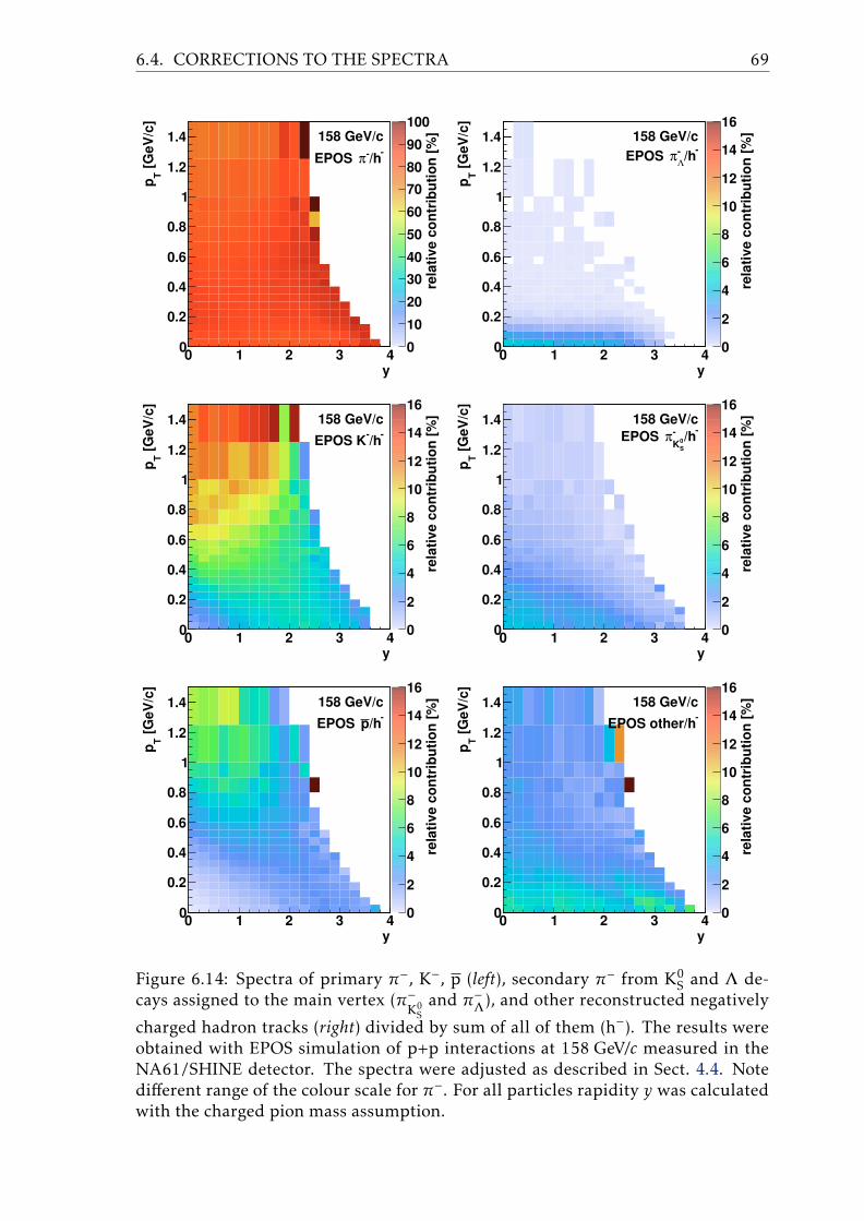
6.4. CORRECTIONS TO THE SPECTRA 69
y0 1 2 3 4
[G
eV
/c]
Tp
0
0.2
0.4
0.6
0.8
1
1.2
1.4
rela
tiv
e c
on
trib
uti
on
[%
]
0
10
20
30
40
50
60
70
80
90
100
-/h-πEPOS
158 GeV/c
y0 1 2 3 4
[G
eV
/c]
Tp
0
0.2
0.4
0.6
0.8
1
1.2
1.4
rela
tiv
e c
on
trib
uti
on
[%
]
0
2
4
6
8
10
12
14
16
-/h
Λ-πEPOS
158 GeV/c
y0 1 2 3 4
[G
eV
/c]
Tp
0
0.2
0.4
0.6
0.8
1
1.2
1.4re
lati
ve
co
ntr
ibu
tio
n [
%]
0
2
4
6
8
10
12
14
16
-/h
-EPOS K
158 GeV/c
y0 1 2 3 4
[G
eV
/c]
Tp
0
0.2
0.4
0.6
0.8
1
1.2
1.4
rela
tiv
e c
on
trib
uti
on
[%
]
0
2
4
6
8
10
12
14
16
-/h
S
0K
-πEPOS
158 GeV/c
y0 1 2 3 4
[G
eV
/c]
Tp
0
0.2
0.4
0.6
0.8
1
1.2
1.4
rela
tiv
e c
on
trib
uti
on
[%
]
0
2
4
6
8
10
12
14
16
-/hpEPOS
158 GeV/c
y0 1 2 3 4
[G
eV
/c]
Tp
0
0.2
0.4
0.6
0.8
1
1.2
1.4
rela
tiv
e c
on
trib
uti
on
[%
]
0
2
4
6
8
10
12
14
16
-EPOS other/h
158 GeV/c
Figure 6.14: Spectra of primary π−, K−, p (left), secondary π− from K0S and Λ de-
cays assigned to the main vertex (π−K0S
and π−Λ), and other reconstructed negatively
charged hadron tracks (right) divided by sum of all of them (h−). The results wereobtained with EPOS simulation of p+p interactions at 158 GeV/c measured in theNA61/SHINE detector. The spectra were adjusted as described in Sect. 4.4. Notedifferent range of the colour scale for π−. For all particles rapidity y was calculatedwith the charged pion mass assumption.

70 CHAPTER 6. DATA ANALYSIS
bins. The track migration effect refers to particles assigned to different (y, pT) or (y,mT) bins than if their true momenta were known, due to finite reconstruction reso-lution. The effect may play a non-negligible role in the regions where the spectrumchanges rapidly between the adjacent bins.
The multiplicative correction closs for losses of inelastic events as well as lossesand track migration of primary π− mesons emitted within the acceptance is calcu-lated using the Monte Carlo simulation as:
closs = n[π−]MCgen / n[π−]MC
sel , (6.10)
where
n[π−]MCgen =
t[π−]MCgen
NMCgen
, (6.11)
where t[π−]MCgen is the number of generated π− tracks in given bin and NMC
gen is thenumber of generated events, while
n[π−]MCsel =
t[π−]MCsel · cacc
NMCsel
, (6.12)
where t[π−]MCsel is the number of reconstructed MC π− tracks selected for the anal-
ysis in given bin and NMCsel is the number of selected events; cacc stands for the
acceptance correction. Then the final, corrected π− meson spectrum in inelasticp+p interactions is calculated as
n[π−] = closs ·nprim[π−] . (6.13)
The dominating effects contributing to the correction closs are
(i) pion migration between bins, cmig,(ii) pion reconstruction inefficiency, ceff,(iii) losses of inelastic events due to the trigger and off-line event selection, csel.
The correction closs can be thus factorised as
closs = cmig · ceff · csel . (6.14)
The correction for pion migration is defined as
cmig = n[π−]MCsel (~p = ~pgen) / n[π
−]MCsel , (6.15)
where n[π−]MCsel (~p = ~pgen) is the reconstructed MC π− spectrum histogrammed using
the simulated momentum, rather than the reconstructed one.The correction for the reconstruction efficiency is defined as
ceff = n[π−]MCgen(S4) / n[π
−]MCsel (~p = ~pgen) , (6.16)
where n[π−]MCgen(S4) is the generated π− spectrum in events passing the event selec-
tion cuts. This includes selection of events with no signal in the S4 counter.Finally the correction for event losses is defined as
csel = n[π−]MCgen / n[π−]MC
gen(S4) . (6.17)
The total correction closs and its contributions cmig, ceff and csel are shown inFig. 6.15.

6.5. STATISTICAL AND SYSTEMATIC UNCERTAINTIES 71
6.4.4 Rejection of poor quality bins of the final spectra
The (y, pT) or (y, mT) bins were removed from the final results in the followingcases:
(i) The relative statistical uncertainty of the bin content is greater than 100%.The reason is to avoid very large biases in the regions of the lowest statistics.
(ii) The relative statistical uncertainty introduced by the MC corrections (includ-ing the h− correction and closs) is greater than 20%. The reason is to minimisesystematic bias introduced by the MC corrections in the regions where theirsystematic uncertainties might be underestimated.
(iii) The bin is isolated in pT or mT from the rest of the spectrum. The missingbins in the middle of the spectra could hinder interpretation of the results bypersons employing them in future analyses.
In all five dataset in total, out of 1148 non-empty (y, pT) RST bins at positive rapid-ity, 5 were rejected due to the criterion (i), 2 due to the criterion (ii) and 1 due tothe criterion (iii).
6.4.5 Total correction
Figure 6.15 shows example magnitudes of corrections applied to the spectra. Thefluctuations that can be observed at 20 GeV/c in particular in the low and the highpT bin occur due to low statistics. This effect is included in the total statisticaluncertainty. The target removed subtraction is in general very small. Correctionfor contamination of particles other than primary π− ranges from −5% to −20%and it is the highest at 158 GeV/c in the high pT region. Correction for event lossesis of order of −10%. The total correction
cTOTAL = n[π−]/nI[h−] (6.18)
typically ranges from −15% to −30%.Figure 6.16 shows the total correction cTOTAL at 20, 31, 40, 80 and 158 GeV/c.
The correction compared at y ≈ 1 and pT ≈ 0.5 GeV/c changes from −15% at20 GeV/c to −25% at 158 GeV/c. This change is mostly caused by the increase ofch− at higher beam momenta due to larger production of particles heavier than π:K−, K0
S, p and Λ.
6.5 Statistical and systematic uncertainties
6.5.1 Statistical uncertainties
Statistical errors receive contributions from the finite statistics of both the dataas well as the simulated events used to obtain the correction factors. The mainassumption was that the numbers of tracks in each bin were undergoing Poissondistribution. This neglects correlations between the tracks in each event, which areexpected to have low impact on the uncertainty.
The dominating contribution is the uncertainty of the measured data which iscalculated in approximation of independent particles. The MC statistics was higherthan the data statistics. Also the uncertainties of the MC corrections calculated

72 CHAPTER 6. DATA ANALYSIS
y0 1 2 3 4
10
0 [
%]
⋅(c
- 1
)
-40
-20
0
20
40
<0.05 [GeV/c]T
0.00<p20 GeV/c
y0 1 2 3 4
10
0 [
%]
⋅(c
- 1
)
-40
-20
0
20
40
<0.05 [GeV/c]T
0.00<p158 GeV/c
y0 1 2 3 4
10
0 [
%]
⋅(c
- 1
)
-40
-20
0
20
40
<0.25 [GeV/c]T
0.20<p20 GeV/c
y0 1 2 3 4
10
0 [
%]
⋅(c
- 1
)
-40
-20
0
20
40
<0.25 [GeV/c]T
0.20<p158 GeV/c
y0 1 2 3 4
10
0 [
%]
⋅(c
- 1
)
-40
-20
0
20
40sub
c
-hc
lossc
mig c
eff c
sel c
TOTALc
<0.70 [GeV/c]T
0.60<p20 GeV/c
y0 1 2 3 4
10
0 [
%]
⋅(c
- 1
)
-40
-20
0
20
40
<0.70 [GeV/c]T
0.60<p158 GeV/c
Figure 6.15: Relative corrections at 20 (left) and 158 GeV/c (right) in selected pTbins. Thick coloured dashed lines show: effective correction from the target re-moved subtraction procedure csub ≡ nT[h
−]/nI[h−] (see Sect. 6.4.1), effective cor-
rection for contribution of particles other than primary π−, ch− ≡ nprim[π−]/nT[h
−](see Sect. 6.4.2) and correction for event and track losses and migration closs (seeSect. 6.4.3) and its contributions cmig, ceff and csel drawn with thin dashed lines.The legend drawn in the bottom left panel concerns all panels. The thick continu-ous black line shows the effective total correction cTOTAL, as defined in Eq. (6.18).A horizontal dashed line at 0 is drawn for reference.

6.5. STATISTICAL AND SYSTEMATIC UNCERTAINTIES 73
)-πy(
0 1 2 3 4
[G
eV
/c]
Tp
0
0.2
0.4
0.6
0.8
1
1.2
1.4
10
0 [
%]
⋅ -
1)
TO
TA
L(c
-40
-30
-20
-10
0
10
20
30
40
-33 -30 -32 -26 -29 -20
-19 -17 -21 -19 -16 -14 -9
-14 -16 -16 -15 -14 -7
-18 -13 -16 -17 -13 -10
-15 -16 -17 -17 -13
-18 -15 -13 -15 -7
-17 -13 -14 -9
-22 -15 -25 -1
-20 -30 -31
20 GeV/c
)-πy(
0 1 2 3 4
[G
eV
/c]
Tp
0
0.2
0.4
0.6
0.8
1
1.2
1.4
10
0 [
%]
⋅ -
1)
TO
TA
L(c
-40
-30
-20
-10
0
10
20
30
40
-22 -24 -25 -28 -28 -21 -17
-17 -17 -20 -20 -18 -16 -13
-14 -16 -17 -16 -15 -13 -8
-15 -16 -18 -16 -14 -14
-14 -16 -16 -15 -14 -10
-17 -17 -15 -15 -10
-17 -17 -16 -12 -13
-16 -15 -15 -8
-20 -18 -4
31 GeV/c
)-πy(
0 1 2 3 4
[G
eV
/c]
Tp
0
0.2
0.4
0.6
0.8
1
1.2
1.4
10
0 [
%]
⋅ -
1)
TO
TA
L(c
-40
-30
-20
-10
0
10
20
30
40
-21 -23 -26 -29 -26 -25 -16
-16 -18 -19 -20 -19 -16 -12
-16 -16 -18 -15 -16 -15 -13
-15 -18 -17 -17 -14 -14 -15
-17 -17 -17 -17 -13 -8
-17 -19 -18 -14 -11 -10
-18 -19 -17 -11 -10
-20 -18 -19 -9
-24 -20 -10
40 GeV/c
)-πy(
0 1 2 3 4
[G
eV
/c]
Tp
0
0.2
0.4
0.6
0.8
1
1.2
1.4
10
0 [
%]
⋅ -
1)
TO
TA
L(c
-40
-30
-20
-10
0
10
20
30
40
-23 -21 -22 -29 -25 -22 -21 -13
-20 -19 -20 -20 -19 -19 -17 -14
-18 -18 -18 -18 -18 -16 -14
-19 -19 -18 -18 -16 -17 -16
-19 -21 -20 -19 -16 -15 -13
-21 -22 -21 -17 -15 -15
-22 -22 -21 -17 -18 -18
-24 -26 -22 -21 -11
-28 -30 -26 -29
80 GeV/c
)-πy(
0 1 2 3 4
[G
eV
/c]
Tp
0
0.2
0.4
0.6
0.8
1
1.2
1.4
10
0 [
%]
⋅ -
1)
TO
TA
L(c
-40
-30
-20
-10
0
10
20
30
40
-23 -24 -22 -24 -25 -20 -19 -22 -14
-21 -22 -21 -22 -22 -20 -19 -17
-21 -21 -22 -22 -20 -22 -18 -13
-21 -22 -22 -21 -21 -21 -19
-24 -24 -24 -22 -21 -22 -20
-25 -25 -25 -23 -21 -20
-28 -27 -27 -24 -22 -21
-29 -30 -29 -25 -26 -21
-36 -33 -32 -35 -30
158 GeV/c
Figure 6.16: The total correction cTOTAL (see Eq. (6.18)) at 20, 31, 40, 80 and158 GeV/c. The numbers printed are averages for each four non-empty adjacentbins.

74 CHAPTER 6. DATA ANALYSIS
assuming binomial distribution are significantly smaller than the uncertainties ofthe number of entries in bins undergoing Poisson distribution.
Statistical uncertainties σnI/R[h
−] of the uncorrected target inserted and removedspectra (Eq. (6.3)) were calculated assuming Poisson probability distribution for thenumber of entries (weighted by the acceptance correction) in a bin:
σn[h−] =
√
∑t[h−]i=1 (ciacc)2
N, (6.19)
where t[h−] is the number of tracks in given bin and ciacc is the acceptance correctioncalculated for each track. For the empty bins in the target removed histograms theuncertainty was calculated assuming a single entry, if at least three (out of eight)adjacent bins were not empty (i.e. they contained any measured tracks). This al-lowed for more realistic estimation of the uncertainties in these bins, without over-estimating them at the far edges of the spectrum, where it is unlikely to find anytracks.
In the subtraction procedure (Eq. (6.4)) the uncertainty was calculated from in-dependent uncertainties of target inserted and removed spectra. Uncertainty of εwas neglected, as it was of order of 1% only (see Table 6.4), and also the resultswere weakly sensitive to its small deviations:
σnT[h
−] =1
1− ε ·√
σ2nI[h
−] + ε ·σ2nR[h
−] . (6.20)
Uncertainty of the additive correction (cV, see Eq. (6.7)) was calculated assumingPoisson distribution of the number of each particle type in given bin:
σcV =
√
√
√∑
x=π−Λ, π−
K0S
, other
σ2n[x] , (6.21)
where the uncertainty of spectrum of particle x (defined in Eq. (6.9)):
σn[x] =
√
t[x] · a[x] · caccN ·∆ . (6.22)
The multiplicative correction (cK, see Eq. (6.8)) is calculated by dividing n[π−]by n[K−]+n[p]+n[π−]. As the component n[π−] dominates over n[K−] and n[p], thenominator and the denominator are strongly correlated. Taking into account thiscorrelation the uncertainty of cK is much smaller than that of cV:
σcK = c2K ·n[K−] +n[p]
n[π−]·
√
√
(
σn[π−]
n[π−]
)2
+σ2n[K−] +σ2
n[p]
(n[K−] +n[p])2. (6.23)
Uncertainty closs (see Eq. (6.10)) was calculated assuming the denominatorn[π−]MC
sel is a subset of nominator n[π−]MCgen and thus undergoes binomial distri-
bution. This assumption is not exactly true as some of the reconstructed tracksassigned to given bin might originate from tracks generated in adjacent bins, due

6.5. STATISTICAL AND SYSTEMATIC UNCERTAINTIES 75
to finite reconstruction resolution and the track migration effect. This effect hasnegligible impact on the uncertainty σcloss . The uncertainty is calculated as follows:
σcloss = closs
√
t[π−]gen − t[π−]selt[π−]gen · t[π−]sel
. (6.24)
Potentially this formula could return nonsense results if the difference in the nom-inator under the square root would be less or equal zero but this has never hap-pened.
The total statistical uncertainty is calculated as:
σstat =[
(
σcloss · cK · (nT[h−]− cV)
)2+(
σcK · closs · (nT[h−]− cV)
)2
+(
σnT[h
−] · cK · closs)2
+(
σcV · cK · closs)2
]1/2,
(6.25)
compare with Eqs. (6.6) and (6.10). The total statistical uncertainty is shown inFigs. 6.17 and 6.18. It is below 1% in the middle of the y–pT phase-space, andstays below 10% except in the bins at the end of the measured spectrum at thelargest y and pT. The uncertainty is larger at the low beam momenta, in particu-lar at 20 GeV/c, due to smaller number of events recorded and smaller number ofparticles produced per event.
6.5.2 Systematic uncertainties
Systematic uncertainties presented in this thesis were calculated independently ineach bin. Figure 6.17 shows the total systematic uncertainties and the contributingeffects, which are listed below.
(i) Possible biases due to event and track cuts which are not corrected for. Theseare:
• a possible bias due to the dE/dx cut applied to remove electrons,• a possible bias related to insufficient rejection of events with off-timebeam particles close in time to the trigger particle.
The magnitude σi of possible biases was estimated by varying values of thecorresponding cuts. The dE/dx cut was shifted by ±0.01 dE/dx units (where1.0 corresponds to minimum ionising particle, and 0.04 is a typical width ofthe dE/dx distribution in small momentum range for π−, K− and p), and theoff-time interactions cut was varied from a ±1 µs to a ±3 µs time window. Asthe two sources of the uncertainty might be correlated the assigned system-atic uncertainty was calculated as the maximum of the absolute differencesbetween the results obtained for both values of the cut. This contribution isdrawn with a long-dashed red line (– –) in Fig. 6.17. This is the dominat-ing source of the systematic uncertainty at the low beammomenta, exceeding10% at the edges of the phase-space. It might be however overestimated inthese regions due to the statistical fluctuations.
(ii) Uncertainty of the correction for contamination of the h− spectra by parti-cles other than primary π− mesons. The systematic uncertainty σii of thiscorrection was assumed as 20% (for 40, 80 and 158 GeV/c) and 40% (for 20

76 CHAPTER 6. DATA ANALYSIS
y0 1 2 3 4
rela
tiv
e u
nc
ert
ain
ty [
%]
0
5
10
15
20
25
30<0.05 [GeV/c]
T0.00<p20 GeV/c
y0 1 2 3 4
rela
tiv
e u
nc
ert
ain
ty [
%]
0
5
10
15
20
25
30
statistical uncertainty
(total, linear sum)linearsysσ
(total, square sum)sysσ
iσ
iiσ
iiiσ
<0.05 [GeV/c]T
0.00<p158 GeV/c
y0 1 2 3 4
rela
tiv
e u
nc
ert
ain
ty [
%]
0
5
10
15
20
25
30<0.25 [GeV/c]
T0.20<p20 GeV/c
y0 1 2 3 4
rela
tiv
e u
nc
ert
ain
ty [
%]
0
5
10
15
20
25
30<0.25 [GeV/c]
T0.20<p158 GeV/c
y0 1 2 3 4
rela
tiv
e u
nc
ert
ain
ty [
%]
0
5
10
15
20
25
30<0.70 [GeV/c]
T0.60<p20 GeV/c
y0 1 2 3 4
rela
tiv
e u
nc
ert
ain
ty [
%]
0
5
10
15
20
25
30<0.70 [GeV/c]
T0.60<p158 GeV/c
Figure 6.17: Statistical and systematic uncertainties in selected pT bins for 20 (left)and 158 GeV/c (right) p+p data. The shaded band shows the statistical uncertainty;at 20 GeV/c the uncertainty exceeds the vertical scale on the plot in several bins. Thecoloured thin lines show the contributions to the systematic uncertainty listed inSect. 6.5.2. The thick black lines show the total systematic uncertainty, which wascalculated by adding the contributions in quadrature (continuous line) or linearly(dashed/dotted line).

6.5. STATISTICAL AND SYSTEMATIC UNCERTAINTIES 77
and 31 GeV/c) of the absolute value of the correction. The increase of the un-certainty at the low beam momenta was arbitrary in order to reflect loweravailability of the reference data to adjust the simulated spectra. This contri-bution is drawn with a dashed-dotted blue line (-···-) in Fig. 6.17. The absolutecorrection is typically of order of −5% to −15% thus the related systematic un-certainty is small.
(iii) Uncertainty of the correction for the event losses. The uncertainty was es-timated using 20% of the correction magnitude and a comparison with thecorrection cVENUS
loss calculated using the VENUS model instead of EPOS:
σiii = 0.2 · |1− closs|+∣
∣
∣closs − cVENUSloss
∣
∣
∣ . (6.26)
This contribution is drawn with a short-dashed green line (- - -) in Fig. 6.17.This uncertainty typically does not exceed 5%.
(iv) Uncertainty related to the track selection method. It was estimated by varyingthe track selection cuts: removing the impact parameter cut and decreasingthe minimum number of required points to 25 (total) and 10 (in VTPCs) andby checking symmetries with respect to y = 0 and pT = 0. The potential biaswas found below 2% and the corresponding contribution was not taken intoaccount in the total systematic uncertainty estimation.
The total systematic uncertainty was calculated by adding the contributions inquadrature:
σsys =√
σ2i +σ2
ii +σ2iii . (6.27)
Finally the systematic uncertainty is averaged between the neighbouring bins. Thereason is that the uncertainty is estimated rather than calculated. Results of thecalculations described above might be overestimated or underestimated due to sta-tistical fluctuations which do not have impact on the actual systematic error of thedata, and are already included in the statistical uncertainty.
The systematic uncertainty is listed in the tables with the numerical values inAppendix C and it is visualised by a shaded band around the data points in plotspresenting the results. Statistical and systematic uncertainties in selected exampleregions are shown in Fig. 6.17. For comparison, the figure includes the alterna-tive systematic uncertainty estimate calculated as a linear sum σ linear
sys = σi+σii+σiii,which is maximum value in case of full correlation of the three contributions. How-ever, as the correlation appears to be unlike, the quadrature sum (Eq. (6.27)) wasused as a final systematic uncertainty estimation.
Systematic biases in different bins are correlated, whereas statistical fluctuationsare almost independent.
In order to calculate the systematic uncertainties of the integrated rapidity spec-tra and of the spectra parameters presented in Chapter 7 (like the inverse slope pa-rameter T or average transverse mass 〈mT〉) the procedure described in this sectionwas repeated independently for each value calculated. As the systematic uncertain-ties are strongly correlated between the adjacent bins it is impossible to propagatethem similarly to the statistical uncertainties.
The total systematic uncertainty σsys is shown in Fig. 6.19. The systematic un-certainty is the lowest in the region of pT from 0.1 GeV/c up to about 0.5 GeV/cbelow the maximum pT measured. It increases at the low pT due to contaminationof the secondary particles, and at the high pT due to contamination of primary K−

78 CHAPTER 6. DATA ANALYSIS
y0 1 2 3 4
[G
eV
/c]
Tp
0
0.2
0.4
0.6
0.8
1
1.2
1.4 [%
]s
tat
σre
lati
ve
0
2
4
6
8
10
12
14
16
18
2020 GeV/c
y0 1 2 3 4
[G
eV
/c]
Tp
0
0.2
0.4
0.6
0.8
1
1.2
1.4 [%
]s
tat
σre
lati
ve
0
2
4
6
8
10
12
14
16
18
2031 GeV/c
y0 1 2 3 4
[G
eV
/c]
Tp
0
0.2
0.4
0.6
0.8
1
1.2
1.4 [%
]s
tat
σre
lati
ve
0
2
4
6
8
10
12
14
16
18
2040 GeV/c
y0 1 2 3 4
[G
eV
/c]
Tp
0
0.2
0.4
0.6
0.8
1
1.2
1.4 [%
]s
tat
σre
lati
ve
0
2
4
6
8
10
12
14
16
18
2080 GeV/c
y0 1 2 3 4
[G
eV
/c]
Tp
0
0.2
0.4
0.6
0.8
1
1.2
1.4 [%
]s
tat
σre
lati
ve
0
2
4
6
8
10
12
14
16
18
20158 GeV/c
Figure 6.18: Relative statistical uncertainty σstat (see Eq. (6.25)) of the π− spectrafor 20, 31, 40, 80 and 158 GeV/c.

6.5. STATISTICAL AND SYSTEMATIC UNCERTAINTIES 79
y0 1 2 3 4
[G
eV
/c]
Tp
0
0.2
0.4
0.6
0.8
1
1.2
1.4 [%
]s
ys
σre
lati
ve
0
2
4
6
8
10
12
14
16
18
2020 GeV/c
y0 1 2 3 4
[G
eV
/c]
Tp
0
0.2
0.4
0.6
0.8
1
1.2
1.4 [%
]s
ys
σre
lati
ve
0
2
4
6
8
10
12
14
16
18
2031 GeV/c
y0 1 2 3 4
[G
eV
/c]
Tp
0
0.2
0.4
0.6
0.8
1
1.2
1.4 [%
]s
ys
σre
lati
ve
0
2
4
6
8
10
12
14
16
18
2040 GeV/c
y0 1 2 3 4
[G
eV
/c]
Tp
0
0.2
0.4
0.6
0.8
1
1.2
1.4 [%
]s
ys
σre
lati
ve
0
2
4
6
8
10
12
14
16
18
2080 GeV/c
y0 1 2 3 4
[G
eV
/c]
Tp
0
0.2
0.4
0.6
0.8
1
1.2
1.4 [%
]s
ys
σre
lati
ve
0
2
4
6
8
10
12
14
16
18
20158 GeV/c
Figure 6.19: Relative systematic uncertainty σsys (see Eq. (6.27)) of the π− spectrafor 20, 31, 40, 80 and 158 GeV/c.

80 CHAPTER 6. DATA ANALYSIS
and p. The uncertainty is the lowest, down to 4%, at 40 GeV/c. It is higher at thelower beam momenta due to higher uncertainty of the h− correction, and at thehigher beam momenta due to the bias introduced by use of the S4 counter. In mostregions it is below 10%, except at 20 GeV/c in the regions of the highest measuredpT where the low statistics limits the precision of the systematic uncertainty calcu-lation.
6.6 Cross checks of the final spectra
6.6.1 Introduction
Validity of the final π− spectra was verified in several tests. First, the expected sym-metries of the spectra were evaluated. Second, the existing measurements of p+pinteractions at 32 GeV/c [71] and 158 GeV/c [25] were compared with the NA61/SHINE results. Also the NA61/SHINE rapidity spectra were compared with theresults at 12 and 24 GeV/c [72] and at 19 GeV/c [73]. This last comparison is ratherinconclusive concerning correctness of the results, but rather reveals difficulty incomparing results obtained at different beam momenta.
The spectra used for the comparisons include all corrections. The method toobtain integrated rapidity spectra and their parametrisation will be explained indetail in Sect. 7.4.
6.6.2 Symmetries of the spectra
Spectra of the particles produced in collisions of non-polarised, identical particlesare expected to obey reflection symmetry with respect to mid-rapidity and rota-tional symmetry around the beam axis. The latter symmetry imposes that the RSTand WST spectra (as defined in Eq. (6.1)) are identical.
As the NA61/SHINE acceptance extends somewhat below mid-rapidity checkof the reflection symmetry can be used to validate the measurements. This check isillustrated in Fig. 6.20, where the fully corrected spectra in y–pT are shown aboveand below mid-rapidity. Yields measured for y < 0 agree within 1.5% with thosemeasured for y > 0 in the reflected acceptance. A similar agreement was also foundat the lower beam momenta. Only the measurements above mid-rapidity are takenas the final results. Nevertheless, for comparison the points at y < 0 are added inFigs. 6.22 and 7.6 in the regions where the measured pT range extends to zero.
Figure 6.20 shows selected WST spectra in full rapidity range. The acceptanceof the wrong side track spectra extends further in the backward rapidity, and a bitin the very forward rapidity. However, as shown in the figure, the acceptance ofthe wrong side tracks misses some regions at the forward rapidity, in particular atthe low beam momenta. The missing regions at low pT at 20 GeV/c and high pT at158 GeV/c correspond to particles passing through the uninstrumented gap aroundthe beam line. Small differences between the forward an backward rapidity, andbetween RST and WST are due to statistical fluctuations.
Figure 6.21 shows ratios of spectra at y > 0 to the spectra reflected with respectto y = 0 and to the wrong side track spectra. The ratios are expected to equal1. The phase-space available for the comparison is very limited, in particular atthe low beam momenta. A bin-by-bin comparison is inconclusive due to statistical

6.6. CROSS CHECKS OF THE FINAL SPECTRA 81
y-4 -3 -2 -1 0 1 2 3 4
[G
eV
/c]
Tp
0
0.2
0.4
0.6
0.8
1
1.2
1.4
0
0.2
0.4
0.6
0.8
1
1.2
1.420 GeV/cright side tracks
y-4 -3 -2 -1 0 1 2 3 4
[G
eV
/c]
Tp
0
0.2
0.4
0.6
0.8
1
1.2
1.4
0
0.2
0.4
0.6
0.8
1
1.2
1.420 GeV/cwrong side tracks
y-4 -3 -2 -1 0 1 2 3 4
[G
eV
/c]
Tp
0
0.2
0.4
0.6
0.8
1
1.2
1.4
0
0.2
0.4
0.6
0.8
1
1.2
1.4158 GeV/cright side tracks
y-4 -3 -2 -1 0 1 2 3 4
[G
eV
/c]
Tp
0
0.2
0.4
0.6
0.8
1
1.2
1.4
0
0.2
0.4
0.6
0.8
1
1.2
1.4158 GeV/cwrong side tracks
Figure 6.20: Fully corrected rapidity and the transversemomentum spectrum of theπ− mesons produced in inelastic p+p interactions at 20 (two top panels) 158 GeV/c(two bottom panels) obtained from the regular right side track analysis and wrongside tracks (marked in the legend). Data below and above mid-rapidity are shownto illustrate reflection symmetry of the measured spectrum with respect to y = 0 (asmarked with the dashed line).

82 CHAPTER 6. DATA ANALYSIS
|y|
0 1 2 3 4
[G
eV
/c]
Tp
0
0.2
0.4
0.6
0.8
1
1.2
1.4
0.8
0.85
0.9
0.95
1
1.05
1.1
1.15
1.2
0.056±a = 1.051
0.030±w = 0.979
20 GeV/cRST
/(y>0)RST
reflected(y<0)
|y|
0 1 2 3 4
[G
eV
/c]
Tp
0
0.2
0.4
0.6
0.8
1
1.2
1.4
0.8
0.85
0.9
0.95
1
1.05
1.1
1.15
1.2
0.009±a = 0.973
0.004±w = 0.986
158 GeV/cRST
/(y>0)RST
reflected(y<0)
y0 1 2 3 4
[G
eV
/c]
Tp
0
0.2
0.4
0.6
0.8
1
1.2
1.4
0.8
0.85
0.9
0.95
1
1.05
1.1
1.15
1.2
0.021±a = 1.004
0.011±w = 0.988
20 GeV/cRST/(y>0)WST(y>0)
y0 1 2 3 4
[G
eV
/c]
Tp
0
0.2
0.4
0.6
0.8
1
1.2
1.4
0.8
0.85
0.9
0.95
1
1.05
1.1
1.15
1.2
0.005±a = 0.967
0.002±w = 0.986
158 GeV/cRST/(y>0)WST(y>0)
|y|
0 1 2 3 4
[G
eV
/c]
Tp
0
0.2
0.4
0.6
0.8
1
1.2
1.4
0.8
0.85
0.9
0.95
1
1.05
1.1
1.15
1.2
0.035±a = 0.994
0.024±w = 1.006
20 GeV/cRST
/(y>0)WST
reflected(y<0)
|y|
0 1 2 3 4
[G
eV
/c]
Tp
0
0.2
0.4
0.6
0.8
1
1.2
1.4
0.8
0.85
0.9
0.95
1
1.05
1.1
1.15
1.2
0.008±a = 0.992
0.005±w = 0.996
158 GeV/cRST
/(y>0)WST
reflected(y<0)
Figure 6.21: Verification of the symmetry between RST and WST and symmetrywith respect to mid-rapidity at 20 (left) and 158 GeV/c (right). The plots of RSTspectra at y < 0 reflected with respect to y = 0 (top), WST spectra (middle) and WSTspectra at y < 0 reflected with respect to y = 0 (bottom) are divided by the RSTspectra at y > 0. All these four spectra are expected to be identical thus the ratiosshould equal 1. Averages of the ratios: arithmetic a and weighted by the statisticaluncertainties w are given in the legend.

6.6. CROSS CHECKS OF THE FINAL SPECTRA 83
fluctuations, however the average difference between the spectra typically does notexceed 2%. This result is consistent with expected symmetries of the spectra withrespect to y = 0 and between WST and RST.
6.6.3 Comparison with existing p+p data at 32 and 158 GeV/c
Figure 6.22 (left) shows a comparison of the rapidity distribution at 31 GeV/c withthe MIRABELLE results at 32 GeV/c [71]. A Gaussian parametrisation of the dis-tribution and the total π− multiplicity are provided. The normalisation of theparametrisation provided in Ref. [71] appears to be incorrect, possibly due to miss-ing factor 1/(σ
√2π) in the Gaussian formula. The discrepancy was solved by nor-
malising the parametrisation shown in Fig. 6.22 to the total multiplicity. The resultsagree within the NA61/SHINE systematic uncertainties.
Figure 6.22 (right) presents a comparison of the rapidity spectrum of the π−
mesons produced in inelastic p+p interactions at 158 GeV/c from the present anal-ysis with the corresponding spectrum measured by NA49 [25]. Statistical and sys-tematic uncertainties of the NA49 spectrum are not explicitly given but the pub-lished information implies that the systematic uncertainty dominates and amountsto several %. The results agree within the systematic uncertainties of the NA61/SHINE spectra.
y-2 0 2
dy
dn
0
0.1
0.2
0.3
0.4
0.5
0.6
0.7NA61/SHINE (31 GeV/c)
MIRABELLE (32 GeV/c)
y-2 0 2
dy
dn
0
0.1
0.2
0.3
0.4
0.5
0.6
0.7
0.8
0.9NA61/SHINE (alternative)
NA61/SHINE
NA49
Figure 6.22: Comparisons of the rapidity distribution of the π−mesons produced ininelastic p+p interactions. Left: The NA61/SHINE results at 31 GeV/c (blue points)are compared with the MIRABELLE measurement (parametrised by the black line)at 32 GeV/c. The shaded band shows the NA61/SHINE systematic uncertainty.Right: Rapidity distribution of the π− mesons produced in inelastic p+p interac-tions at 158 GeV/c. The large blue points show the results obtained with an alter-native method: without vertex fit requirement and rejection of events with a singlevery high momentum positively charged track. The results of NA61/SHINE (reddots) are compared with the NA49 measurements [25] (black squares). The opensymbols show points reflected with respect to mid-rapidity. A single NA61/SHINEpoint measured at y < 0 is also shown for comparison. The shaded band shows theNA61/SHINE systematic uncertainty.

84 CHAPTER 6. DATA ANALYSIS
The analysis method of p+p interactions at 158 GeV/c performed by NA49 [25]differed from the one used in this thesis. In particular, pions were identified bydE/dx measurement and the NA49 event selection criteria did not include the se-lection according to the fitted z coordinate of the interaction vertex and the rejec-tion of elastic interactions. Namely, all events passing the trigger selection andoff-line quality cuts were used for the analysis. For comparison, this event selectionprocedure was applied to the NA61/SHINE data. As a result 20%more events wereaccepted. Approximately half of them were the elastic and off-target interactionsand half were required inelastic interactions. Then the corrections correspondingto the changed selection criteria were applied (the contribution of elastic events wassubtracted using the estimate from Ref. [25]). The fully corrected rapidity spectrumobtained using this alternative analysis is also shown in Fig. 6.22 (right). The differ-ences between the results for the standard and alternative methods are below 0.5%at y < 2 and below 2% at higher y.
It should be noted that the complete NA49 normalisation method could not beused with the NA61/SHINE due to the difficulties with deriving the cross sectionsrelated to the uncertainty of the target removed to inserted ratio (see Sect. 5.3). Thecross-sections used in the normalisation of the alternative analysis of the 158 GeV/cdata, drawn with the blue points in Fig. 6.22 (right) were taken from the NA49analysis in Ref. [25]. Corresponding cross-sections for the lower momenta of thebeam particles are not available.
6.6.4 Comparison with existing p+p data at 12, 19 and 24 GeV/c
In this section the results of NA61/SHINE are compared with the bubble chamberresults from p+p collisions at 12 and 24 GeV/c [72] and at 19 GeV/c [73]. The ref-erence data were available only in form of histograms. The data points were readoff from the scanned figures. In case the error bars were not visible, the printedpoint size was assumed as the uncertainty. This concerns several points in themid-rapidity region in the 12 and 24 GeV/c datasets; their uncertainties are over-estimated.
As the results of NA61/SHINE are obtained at different beam momenta, thecomparison has to involve model-based scaling or interpolation. Two approacheswere considered.
In the first approach a limiting fragmentation model [74] was assumed. Themodel predicts that the rapidity spectra in the laboratory frame of reference do notdepend on the beam momentum in the region close to yLAB(≡ y + yCMS) � 0. Fig-ure 6.23 shows the NA61/SHINE results reflected with respect to y = 0 and trans-formed to the laboratory frame of reference. A function fitted to the 158 GeV/cpoints was used as a reference; the choice is arbitrary and does not affect the com-parison. In general the particle yields in this region increase with decreasing beammomentum, thus the limiting fragmentationmodel is not valid for p+p interactionsat the SPS energy range. The largest difference is observed at yLAB = −0.5. The 20and 31 GeV/c data lie, respectively, 40% and 10% above the 24 GeV/c data. Thiscould naively be interpreted as an inconsistency between the NA61/SHINE andthe bubble chamber data. The 19 GeV/c reference data do not lie between the 12and 24 GeV/c data. This can be partially explained by large statistical uncertainties

6.6. CROSS CHECKS OF THE FINAL SPECTRA 85
LABy
-1 -0.5 0 0.5
LA
Bd
n/d
y
0
0.1
0.2
0.3
0.4
0.5
0.6p+p at 158 GeV/c (with fit)p+p at 80 GeV/cp+p at 40 GeV/cp+p at 31 GeV/cp+p at 24 GeV/c (Blobel et al.)p+p at 20 GeV/cp+p at 19 GeV/c (Boeggild et al.)p+p at 12 GeV/c (Blobel et al.)
LABy
-1 -0.5 0 0.5
15
8d
ata
/fit
0.6
0.8
1
1.2
1.4
1.6
1.8
2
Figure 6.23: Comparison of the rapidity spectra from this thesis (filled symbols)with the p+p data at 12 and 24 GeV/c from Ref. [72] (Blobel et al., open symbols)and with the p+p data at 19 GeV/c from Ref. [73] (Bøggild et al., black stars). Left:The rapidity spectra in the laboratory frame of reference. The 158 GeV/c spectrumwas fitted with the double Gaussian function (solid line, see Eq. (7.2)) in the re-gion corresponding to y > 2 in the centre of mass frame; the dashed line showsextrapolated function. Right: the spectra divided by the fitted function, also in theextrapolated region. The data points were connected with lines to guide an eye.
of the data points, but also demonstrates inconsistency between results of variousexperiments.
In the second approach the comparison was done assuming scaling of the shapeof rapidity spectra in relative rapidity y/ybeam. Figure 6.24 (top) shows the spectrain the relative rapidity normalised to unity in order to exclude trivial effect of anincrease of mean pion multiplicity with collision energy. The data measured at 12and 24 GeV/c are compared with the parametrised NA61/SHINE results at 20 (left)and 31 GeV/c (right). The ratios of the 12 and 24 GeV/c spectra to the NA61/SHINEfits are shown in the corresponding bottom panels. The spectra at y/ybeam < 0.7agree better than 10%. At the higher rapidities however, the differences increaseto almost 100%, both between the results from this thesis and the reference data,and between the reference data at different beammomenta. The 20 GeV/c points liebetween the 12 and 24 GeV/c ones, while the 31 GeV/c lie below 24 GeV/c. Thus thiscomparison of the spectra does not indicate any inconsistency between them. In theregion of y/ybeam > 0.7 the 19 GeV/c points lie between the 12 and 24 GeV/c points,closer to the 24 GeV/c points, which is consistent, as opposed to the comparisonusing the limiting fragmentation model scaling.
The two comparisons clearly demonstrate trivial fact that an interpolation be-tween measurements may be strongly model dependent and lead to a significantbias. In the considered two examples even the qualitative conclusion whether ornot the data are consistent depends on the model used for the comparison. Thisconfirms importance of the NA61/SHINE scan of collisions of various ions at thesame beam momenta. In particular the p+p data cannot be obtained by interpolat-

86 CHAPTER 6. DATA ANALYSIS
beamy/y
0 0.5 1 1.5 2
⟩-
π⟨ /
)b
ea
md
(y/yd
n
-410
-310
-210
-110
1
p+p at 12 GeV/c (Blobel et al.)p+p at 19 GeV/c (Boeggild et al.)p+p at 24 GeV/c (Blobel et al.)p+p at 20 GeV/c (NA61)
beamy/y
0 0.5 1 1.5 2
refe
ren
ce / N
A61
0
0.2
0.4
0.6
0.8
1
1.2
1.4
1.6
1.8
2
beamy/y
0 0.5 1 1.5 2
⟩-
π⟨ /
)b
ea
md
(y/yd
n
-410
-310
-210
-110
1
p+p at 12 GeV/c (Blobel et al.)p+p at 19 GeV/c (Boeggild et al.)p+p at 24 GeV/c (Blobel et al.)p+p at 31 GeV/c (NA61)
beamy/y
0 0.5 1 1.5 2
refe
ren
ce / N
A61
0
0.2
0.4
0.6
0.8
1
1.2
1.4
1.6
1.8
2
Figure 6.24: Comparison of the normalised rapidity spectra from this thesis (pa-rametrised with a line) at 20 (left) and 31 GeV/c (right) with the p+p data at 12and 24 GeV/c from Ref. [72] (Blobel et al., open symbols) and with the p+p data at19 GeV/c from Ref. [73] (Bøggild et al., green stars). The top panels show the spectraand the bottom panels show the 12, 19 and 24 GeV/c spectra divided by the param-etrised results from this thesis. The vertical dashed line at the ratio of 1 is drawnfor reference. The data points were connected with solid lines to guide an eye.
ing the existing results. Also the data cannot be validated by comparison to datataken at different collision energies.

Chapter 7
π− spectra in p+p interactions andcomparisons with Pb+Pb data andsimulations
7.1 Introduction
This chapter presents results on inclusive π− meson spectra in inelastic p+p in-teractions at beam momenta of 20, 31, 40, 80 and 158 GeV/c. The spectra referto pions produced by strong processes and in electromagnetic decays of producedhadrons. They are corrected for all effects related to detection and reconstruction,as described in Chapter 6.
Numerical results corresponding to the plotted spectra as well as their statisticaland systematic uncertainties are given in Appendix C, as well in Ref. [29] in plaintext format and in ROOT format.
The results are compared with existing p+p data [25, 63, 71, 75] and with thecorresponding data on central Pb+Pb collisions at the same beam momenta pernucleon (except of 30A GeV/c instead of 31 for Pb+Pb) published by NA49 [8, 9],as well as results on central Au+Au collisions from AGS [76, 77] and RHIC [78–82], as processed in Ref. [9]. Here, centrality is a parameter determining numberof nucleons of the projectile and the target nuclei participating in the collision.The central collisions selected by NA49 refer to 7% (5%) of the collisions at 20–80A GeV/c (158A GeV/c) for which the number of participating nucleons was thehighest. Pion production characteristics in p+p interactions and central Pb+Pbcollisions are identified and compared.
The chapter ends with comparisons of the measured π− spectra with predictionsof theoretical models: EPOS and VENUS.
7.2 Double differential spectra
The double differential spectra derived in bins of rapidity and the transverse mo-mentum d2n/(dydpT), and rapidity and the transverse mass d2n/(dydmT) are equalto the fully corrected bin contents n[π−] defined in Eq. (6.13). The spectra in rapid-ity and the transverse momentum produced in inelastic p+p interactions at 20, 31,40, 80 and 158 GeV/c are shown in Fig. 7.1.

88 CHAPTER 7. π− SPECTRA IN P+P INTERACTIONS ANDCOMPARISONS . . .
y0 1 2 3 4
[G
eV
/c]
Tp
0
0.2
0.4
0.6
0.8
1
1.2
1.4
0
0.2
0.4
0.6
0.8
1
1.2
1.420 GeV/c
y0 1 2 3 4
[G
eV
/c]
Tp
0
0.2
0.4
0.6
0.8
1
1.2
1.4
0
0.2
0.4
0.6
0.8
1
1.2
1.431 GeV/c
y0 1 2 3 4
[G
eV
/c]
Tp
0
0.2
0.4
0.6
0.8
1
1.2
1.4
0
0.2
0.4
0.6
0.8
1
1.2
1.440 GeV/c
y0 1 2 3 4
[G
eV
/c]
Tp
0
0.2
0.4
0.6
0.8
1
1.2
1.4
0
0.2
0.4
0.6
0.8
1
1.2
1.480 GeV/c
y0 1 2 3 4
[G
eV
/c]
Tp
0
0.2
0.4
0.6
0.8
1
1.2
1.4
0
0.2
0.4
0.6
0.8
1
1.2
1.4158 GeV/c
Figure 7.1: Double differential spectra d2n/(dydpT) [(GeV/c)−1] of the π− mesonsproduced in inelastic p+p interactions at 20, 31, 40, 80 and 158 GeV/c.

7.3. TRANSVERSE MASS SPECTRA 89
]2 [GeV/cπ - mT
m
0 0.5 1
]-2 )
2 [
(Ge
V/c
Td
y d
mn2
d
Tm1
3−10
2−10
1−10
1
10
210
16×
8×
4×2×
158 GeV/c
80 GeV/c
40 GeV/c
31 GeV/c
20 GeV/c
Figure 7.2: Transverse mass spectra atmid-rapidity (0 < y < 0.2). The fitted ex-ponential function Eq. (7.1) is indicatedby solid lines in the fit range 0.2 < (mT −mπ) < 0.7 GeV/c2 and dashed lines out-side the fit range. The data points fordifferent beam momenta were scaled forbetter readability.
Table 7.1: Numerical values of the parameters fitted to the transverse mass spectra(see Eq. (7.1)) of the π− mesons produced in inelastic p+p interactions at 20, 31,40, 80 and 158 GeV/c. The uncertainty values provided correspond to the statisticaland systematic uncertainties, respectively.
pbeam [GeV/c] T(y = 0) [MeV/c2] 〈mT〉(y = 0)−mπ [MeV/c2]20 149.1± 5.0± 4.8 237.8± 6.4± 2.331 153.3± 2.2± 1.2 246.1± 2.7± 0.940 157.7± 1.7± 2.1 247.3± 2.0± 0.980 159.9± 1.5± 4.1 253.5± 1.9± 1.1158 159.3± 1.3± 2.6 253.6± 1.6± 1.4
7.3 Transverse mass spectra
Figure 7.2 shows the transverse mass spectra at mid-rapidity (0 < y < 0.2). A func-tion
dn
dmT= A ·mT · exp
(
−mT
T
)
(7.1)
was fitted in the range 0.2 < (mT −mπ) < 0.7 GeV/c2 and is indicated by lines inFig. 7.2. The normalisation coefficient A and the inverse slope T were the fittedparameters. The fit minimises the χ2 function calculated using statistical errorsonly. In the χ2 calculation for each bin the measured bin content (dn/dmT) wascompared with integral of the fitted function over the bin, divided by the bin width.The fitmT range was chosen the same as for the Pb+Pb results [8,9] in order to allowfor comparison.
Table 7.1 lists the fitted values of T at mid-rapidity, and the mean transversemass 〈mT〉. In order to calculate 〈mT〉 the spectra were extrapolated exponentiallybeyond themeasured part of highmT spectrum. The extrapolated function togetherwith the measured data was used to calculate the 〈mT〉 value, see Appendix B.1 fordetails. Half of the resulting correction is added to the systematic uncertainty inquadrature.
Figure 7.3 shows the inverse slope parameter T (left) and the mean transversemass (right) calculated in all rapidity bins containing sufficient measured points.

90 CHAPTER 7. π− SPECTRA IN P+P INTERACTIONS ANDCOMPARISONS . . .
beamy/y
0 0.2 0.4 0.6 0.8 1
]2
T [
Me
V/c
80
90
100
110
120
130
140
150
160
170
158 GeV/c
80 GeV/c
40 GeV/c
31 GeV/c
20 GeV/c
beamy/y
0 0.5 1 1.5
]2
[G
eV
/cπ
-m⟩T
m⟨
0
0.05
0.1
0.15
0.2
0.25
0.3
158 GeV/c
80 GeV/c
40 GeV/c
31 GeV/c
20 GeV/c
Figure 7.3: Left: The inverse slope parameter T of the transverse mass spectra as afunction of rapidity divided by the projectile rapidity ybeam( = 1.877, 2.094, 2.223,2.569 and 2.909 at 20, 31, 40, 80 and 158 GeV/c, respectively). The fit range is0.2 < (mT −mπ) < 0.7 GeV/c2. Right: The mean transverse mass 〈mT〉 as a functionof rapidity divided by the projectile rapidity. The results in both panels refer to theπ− mesons produced in inelastic p+p interactions at 20, 31, 40, 80 and 158 GeV/c.
]2 [GeV/cπ - mT
m
0 0.2 0.4 0.6 0.8 1
(Pb
+P
b)/
(p+
p)
0
0.2
0.4
0.6
0.8
1
1.2
1.4
1.6
1.8
2
GeV/cA158
GeV/cA80
GeV/cA40
GeV/cA31
GeV/cA20
Figure 7.4: Ratio of the normalisedtransverse mass spectra of the π−mesonsat mid-rapidity produced in centralPb+Pb collisions and inelastic p+p in-teractions at the same collision energyper nucleon. The systematic uncertaintyof the ratio represented by the colouredbands was calculated using uncertaintyof the p+p data only.
For all beammomenta both parameters decrease significantly with rapidity increas-ing from mid-rapidity to the projectile rapidity ybeam. For y/ybeam < 1 they increaseslightly with increasing beam momentum, but shape of the dependence on y/ybeamis rather similar at all energies.
Figure 7.4 shows ratio of the transverse mass spectra of the π−mesons producedat mid-rapidity (0 < y < 0.2) in central Pb+Pb collisions and p+p interactions at thesame collision energy per nucleon. As the Pb+Pb data at 40, 80 and 158 GeV/c wasderived in different bins of mT, the Pb+Pb points were interpolated to the binningused in this thesis assuming exponential behaviour, as in Eq. (7.1). The spectrawere normalised to unity before calculating the ratio. The ratio is not constantimplying the the spectral shapes are different in p+p interactions and central Pb+Pbcollisions. Also, the ratio does not depend on the collision energy. The ratio is larger

7.4. RAPIDITY SPECTRA 91
[GeV]NN
s
6 7 8 9 10 20
]2
T [
Me
V/c
140
150
160
170
180
190
200p+p (SPS - NA61/SHINE)
Pb+Pb (SPS)
[GeV]NN
s1 10
210
]2
[G
eV
/cπ
- m
⟩T
m⟨
0
0.05
0.1
0.15
0.2
0.25
0.3
0.35
0.4
p+p (SPS - NA61/SHINE)
Au+Au (AGS)
Pb+Pb (SPS)
Au+Au (RHIC)
Figure 7.5: Left: Inverse slope parameter T of the transverse mass spectra at mid-rapidity (0 < y < 0.2) plotted against the collision energy per nucleon. The param-eter T was fitted in the range 0.2 < (mT −mπ) < 0.7 GeV/c2. The systematic uncer-tainty is shown with faded bands. As for the two lowest energy points for Pb+Pb,the systematic uncertainty was not given in [9], it is assumed to be the same asfor the higher energies [8]. Right: The mean transverse mass 〈mT〉 at mid-rapidity(0 < y < 0.2) versus the collision energy. The results on inelastic p+p interactionsare compared with the corresponding data on central Pb+Pb and Au+Au collisions.
than unity for (mT −mπ) < 0.1 GeV/c2 and (mT −mπ) > 0.5 GeV/c2. It is smaller thanunity in the region of 0.1 < (mT −mπ) < 0.5 GeV/c2.
Figure 7.5 (left) shows the inverse slope parameter T of the transverse massspectra at mid-rapidity as a function of the collision energy. The T parameter islarger by about 10–20 MeV/c2 in central Pb+Pb collisions than in p+p interactions.Figure 7.5 (right) shows comparison for the mean transverse mass 〈mT〉 parameterin the p+p and Pb+Pb data. In spite of different shapes of the mT spectra, 〈mT〉is similar. This is because the differences in shapes of the mT spectra at low mT
and high mT shown in Fig. 7.4 cancel each other when calculating 〈mT〉. Thus,the mean transverse mass appears to be insensitive to the apparent changes of thepion production properties observed between p+p interactions and central Pb+Pbcollisions.
7.4 Rapidity spectra
Figure 7.6 shows the rapidity spectra. They were obtained by summing the mT
spectra in the measured range with the exponential function Eq. (7.1) extrapolatingthe spectrum (see Appendix B.1 for details). The correction is typically below 0.2%and becomes significant (a few %) only at y > 2.4. Half of the correction is added inquadrature to the systematic uncertainty.
The pion yield increases with increasing collision energy at all measured rapidi-ties.
The rapidity spectra are approximately Gaussian, but as demonstrated in Ap-pendix B.2, sum of two Gaussian functions symmetrically displaced with respect

92 CHAPTER 7. π− SPECTRA IN P+P INTERACTIONS ANDCOMPARISONS . . .
y-2 0 2
dy
dn
0
0.1
0.2
0.3
0.4
0.5
0.6
0.7
0.8158 GeV/c
80 GeV/c
40 GeV/c
31 GeV/c
20 GeV/c
Figure 7.6: Rapidity spectra obtainedfrom sums of the measured and extrap-olated mT spectra. Closed symbols in-dicate measured points, open points arereflected with respect to y = 0. Themeasured points at y < 0 are shown forsystematic comparison only. The plot-ted statistical errors are almost alwayssmaller than the symbol size. The sys-tematic uncertainties are indicated bythe coloured bands. The lines indicatefits of function Eq. (7.2) to the spectra.The results refer to the π− mesons pro-duced in inelastic p+p interactions at 20,31, 40, 80 and 158 GeV/c.
Table 7.2: Numerical values of the parameters fitted to rapidity spectra (seeEq. (7.2)) of the π− mesons produced in inelastic p+p interactions at 20, 31, 40,80 and 158 GeV/c. As the systematic uncertainty dominates over the statistical one,the uncertainties written in the table are the square root of sum of squares of thestatistical and systematic uncertainties. All uncertainties are given numerically inAppendix C.2.
pbeam [GeV/c] 〈π−〉 σ σ0 y020 1.047± 0.051 0.981± 0.017 0.921± 0.118 0.337± 0.40631 1.312± 0.069 1.031± 0.016 0.875± 0.050 0.545± 0.05540 1.478± 0.051 1.069± 0.014 0.882± 0.045 0.604± 0.04480 1.938± 0.080 1.189± 0.026 0.937± 0.019 0.733± 0.010158 2.444± 0.130 1.325± 0.042 1.007± 0.051 0.860± 0.021
to mid-rapidity gives much better description:
dn
dy=〈π−〉(y0,σ0)2σ0√2π
·[
exp
(
−(y − y0)2
2σ20
)
+ exp
(
−(y + y0)2
2σ20
)]
. (7.2)
The y0 and σ0 are fit parameters, and the total multiplicity 〈π−〉(y0,σ0) is calculatedfrom the requirement that the integral over the measured spectrum equals the in-tegral of the fitted function Eq. (7.2) in the range covered by the measurements (seeAppendix B.2 for details). The χ2 function was minimised in a similar way as incase of the mT spectra, using the integral of the function in given rapidity bin. The
numerical values of the fitted parameters as well as the RMS width σ =√
y20 +σ20
are given in Table 7.2. The fitted parameters y0 and σ0 are strongly anticorrelated.As a result their individual uncertainties are large, while the value of σ is weaklysensitive to small deviations of the fit and its uncertainty is much smaller.
Figure 7.7 (left) presents ratio of the normalised π− rapidity spectra producedin central Pb+Pb and inelastic p+p interactions at the same collision energy pernucleon. The spectra are plotted versus normalised rapidity. The ratio is closeto unity in the central rapidity region (y/ybeam < 0.6), whereas it is higher for the

7.5. MEAN MULTIPLICITY 93
beamy/y
0 0.5 1 1.5
(Pb
+P
b)/
(p+
p)
0.6
0.8
1
1.2
1.4
GeV/cA158
GeV/cA80
GeV/cA40
GeV/cA31
GeV/cA20
[GeV]NN
s
6 7 8 9 10 20
σ
0.9
1
1.1
1.2
1.3
1.4
1.5p+p (SPS - NA61/SHINE)
p+p (world)
Pb+Pb (SPS)
Figure 7.7: Left: Ratio of normalised rapidity spectra of the π− mesons producedin central Pb+Pb collisions and inelastic p+p interactions at the same collisionenergy per nucleon plotted versus the rapidity scaled by the beam rapidity. Thecoloured bands represent the NA61/SHINE systematic uncertainty. Right: Energydependence of the width of the rapidity distribution of the π− mesons produced inp+p interactions and central Pb+Pb collisions. The systematic uncertainty for thePb+Pb points is not given.
rapidity approaching the beam rapidity (y/ybeam > 0.6). The energy dependence ofthe ratio is small in comparison to the systematic uncertainties: at y/ybeam < 0.3the ratio increases by 10–20% from 20A to 158 GeV/c; at y/ybeam > 0.5 the ratiodecreases by about 20% from 20A to 158A GeV/c.
Consequently, the RMS width σ of the rapidity distributions of the π− mesonsproduced in p+p interactions is smaller than in central Pb+Pb collisions, as shownin Fig. 7.7. Additionally, p+p data from Refs. [25,71,75] are shown; they agree withthe NA61/SHINE results.
7.5 Mean multiplicity
Mean multiplicities of the π− mesons, 〈π−〉, produced in inelastic p+p interactionsat 20, 31, 40, 80 and 158 GeV/c were calculated using Eq. (7.2). The extrapolationinto the unmeasured region at large y contributes below 2% (see Appendix. B.2).Half of it is added in quadrature to the systematic uncertainty. The 〈π−〉 values aregiven in Table 7.2
Figure 7.8 shows the dependence of the produced average 〈π−〉multiplicity perinelastic p+p collision on the Fermi energy
F ≡[
(√sNN − 2mN)
3
√sNN
]1/4
≈ s1/4NN , (7.3)
where√sNN is energy per nucleon available in centre of mass. Reference [2] predicts
a linear dependence of the pion multiplicity in function of F. The results of NA61/SHINE are in agreement with a compilation of the world data [25,63].

94 CHAPTER 7. π− SPECTRA IN P+P INTERACTIONS ANDCOMPARISONS . . .
]1/2F [GeV
0 1 2 3 4 5
⟩-
π⟨
0
0.5
1
1.5
2
2.5
3NA61/SHINE
world data
Figure 7.8: Dependence of the mean to-tal multiplicity of the π− mesons pro-duced in inelastic p+p interactions onFermi energy F (see Eq. (7.3)). The re-sults of NA61/SHINE are indicated byfilled circles and the compilation of theworld data [25, 63] by open circles. Thestatistical errors are smaller than thesymbol size. The systematic uncertain-ties are indicated by the coloured band.
]1/2F [GeV
0 1 2 3 4 5
⟩W
N⟨/⟩π⟨
0
1
2
3
4
5
6
7
8p+p (SPS - NA61/SHINE)
p+p (world)
Au+Au (AGS)
Pb+Pb (SPS)
Au+Au (RHIC)
Figure 7.9: Mean multiplicity of all pi-ons per wounded nucleon produced ininelastic p+p interactions and centralPb+Pb (Au+Au) collisions. The verti-cal lines show the total uncertainty, cal-culated as a square root of sum of thesystematic and statistical (much smaller)uncertainties. To guide an eye, a lineconnects the ion-ion results, and sepa-rately the p+p results from this thesis.
Note, that the isospin effects should be taken into account in interpretationof differences between results obtained for inelastic p+p interactions and centralPb+Pb collisions. In order to reduce influence of the isospin effects the mean mul-tiplicity of pions is obtained from a sum of mean multiplicities of negatively andpositively charged pions using the phenomenological formula [28]:
〈π〉 = 3
2(〈π+〉+ 〈π−〉) . (7.4)
The mean π multiplicities are shown in Fig. 7.9 as a function of the Fermi energy F(see Eq. (7.3)). They are divided by the mean number of wounded nucleons, definedas the number of nucleons interacting inelastically (NW = 2 for p+p). The value of〈π+〉 for the NA61/SHINE results on inelastic p+p interactions was estimated fromthe measured 〈π−〉 multiplicity assuming 〈π+〉 = 〈π−〉 + 2/3. This assumption isbased on the compilation of the world data presented in Ref. [28] and the modelpresented therein.
At the beammomenta lower than 40A GeV/c (F < 2.5 GeV1/2) the 〈π〉/〈NW 〉 ratiois higher in p+p interactions than in central Pb+Pb collisions. The opposite relationholds for beam momenta larger than 40A GeV/c. The energy dependence of thetotal π multiplicity for inelastic p+p interactions crosses the one for central Pb+Pb(Au+Au) collisions at about 40A GeV/c.

7.6. COMPARISON WITH SIMULATED SPECTRA 95
7.6 Comparison with simulated spectra
Figures 7.10 and 7.11 compare the π− spectra generated by, respectively, EPOS andVENUS models and results of the data analysis. Both models overestimate the π−
production in the low pT and high y region, and underestimate it at high pT. TheVENUS spectra are almost twice too large at rapidities between 2.5 and 3.5. TheEPOS spectra agree better with data in general except at the lowest beam momentawhere the π− yield at high pT is 50% too small. This is consistent with the fact thatEPOS is a newer and better developed model. The EPOS spectra agree with datawithin ±20% at 158 GeV/c and within ±50% at 20 GeV/c.

96 CHAPTER 7. π− SPECTRA IN P+P INTERACTIONS ANDCOMPARISONS . . .
y0 1 2 3 4
[G
eV
/c]
Tp
0
0.2
0.4
0.6
0.8
1
1.2
1.4
0
0.2
0.4
0.6
0.8
1
1.2
1.4
1.6
1.8
220 GeV/c
EPOS/data
y0 1 2 3 4
[G
eV
/c]
Tp
0
0.2
0.4
0.6
0.8
1
1.2
1.4
0
0.2
0.4
0.6
0.8
1
1.2
1.4
1.6
1.8
231 GeV/c
EPOS/data
y0 1 2 3 4
[G
eV
/c]
Tp
0
0.2
0.4
0.6
0.8
1
1.2
1.4
0
0.2
0.4
0.6
0.8
1
1.2
1.4
1.6
1.8
240 GeV/c
EPOS/data
y0 1 2 3 4
[G
eV
/c]
Tp
0
0.2
0.4
0.6
0.8
1
1.2
1.4
0
0.2
0.4
0.6
0.8
1
1.2
1.4
1.6
1.8
280 GeV/c
EPOS/data
y0 1 2 3 4
[G
eV
/c]
Tp
0
0.2
0.4
0.6
0.8
1
1.2
1.4
0
0.2
0.4
0.6
0.8
1
1.2
1.4
1.6
1.8
2158 GeV/c
EPOS/data
Figure 7.10: Double differential spectra of the π− mesons produced in inelasticp+p interactions at 20, 31, 40, 80 and 158 GeV/c generated by EPOS divided by theNA61/SHINE measurement results.

7.6. COMPARISON WITH SIMULATED SPECTRA 97
y0 1 2 3 4
[G
eV
/c]
Tp
0
0.2
0.4
0.6
0.8
1
1.2
1.4
0
0.2
0.4
0.6
0.8
1
1.2
1.4
1.6
1.8
220 GeV/c
VENUS/data
y0 1 2 3 4
[G
eV
/c]
Tp
0
0.2
0.4
0.6
0.8
1
1.2
1.4
0
0.2
0.4
0.6
0.8
1
1.2
1.4
1.6
1.8
231 GeV/c
VENUS/data
y0 1 2 3 4
[G
eV
/c]
Tp
0
0.2
0.4
0.6
0.8
1
1.2
1.4
0
0.2
0.4
0.6
0.8
1
1.2
1.4
1.6
1.8
240 GeV/c
VENUS/data
y0 1 2 3 4
[G
eV
/c]
Tp
0
0.2
0.4
0.6
0.8
1
1.2
1.4
0
0.2
0.4
0.6
0.8
1
1.2
1.4
1.6
1.8
280 GeV/c
VENUS/data
y0 1 2 3 4
[G
eV
/c]
Tp
0
0.2
0.4
0.6
0.8
1
1.2
1.4
0
0.2
0.4
0.6
0.8
1
1.2
1.4
1.6
1.8
2158 GeV/c
VENUS/data
Figure 7.11: Double differential spectra of the π− mesons produced in inelasticp+p interactions at 20, 31, 40, 80 and 158 GeV/c generated by VENUS divided bythe NA61/SHINE measurement results.

Chapter 8
Summary and outlook
This thesis presents experimental results on inclusive spectra and mean multiplici-ties of negatively charged pions produced in inelastic p+p interactions at 20, 31, 40,80 and 158 GeV/c by strong interaction processes and in electromagnetic decays ofproduced hadrons. The measurements were performed using the large acceptanceNA61/SHINE hadron spectrometer at the CERN Super Proton Synchrotron basedon a system of five Time Projection Chambers. Two-dimensional spectra were de-termined in terms of rapidity and transverse momentum or transverse mass withstatistical and systematic uncertainties below 10% in large part of the phase-space.Characteristics of the spectra such as the width of rapidity distributions σ and theinverse slope parameter T of the transverse mass spectra were extracted and theircollision energy dependences were presented.
The results were obtained by deriving spectra of unidentified negatively chargedhadrons and removing contribution of hadrons other than primary π− using EPOSsimulation adjusted based on existing experimental data. Magnitudes of possiblebiases introduced by this and other corrections applied in the analysis were studiedand included in the systematic uncertainty.
The results agree with the existing measurements of p+p interactions fromMIR-ABELLE at 32 GeV/c [71] and NA49 at 158 GeV/c [25] and other experiments [63].In majority of the existing datasets low statistics limits possibilities to study prop-erties of the spectra. The NA61/SHINE measurement provide detailed spectra de-rived in broad phase-space region.
Comparison with the spectra predicted by the EPOS and VENUSmodels revealsdifferences of up to factor of 2. The obtained results might serve as a reference toimprove the models.
The π− spectra in p+p interactions belong to the NA61/SHINE programme of atwo-dimensional scan of the collision energy and in the system size to study prop-erties of onset of deconfinement. They were compared with the data on centralPb+Pb collisions at the same beam momenta per nucleon obtained by the NA49experiment. The spectra in p+p interactions are narrower both in rapidity and inthe transverse mass, which however might be related to isospin effects. The meanpion multiplicity per wounded nucleon in p+p interactions increases slower withenergy in the SPS range and crosses the corresponding dependence measured inthe Pb+Pb collisions at about 40A GeV/c, which supports interpretation of the on-set of deconfinement in Pb+Pb collisions. Surprisingly, the energy dependences of


Appendix A
Coordinate system and kinematicvariables
A.1 Introduction
This appendix introduces the standard detector coordinate system used in this the-sis as well as the definition of the kinematic variables. The reconstruction algo-rithms calculate the momentum vector of each particle at the interaction vertex.Various kinematic variables used in this thesis facilitate analysis of various trackcharacteristics.
A.2 NA61/SHINE coordinate system
The coordinate system used in NA61/SHINE and in this thesis is shown in Fig. 2.1on page 9. The origin of the system is located in the centre of VTPC-2, on the beamline. The system is right-handed. The z axis is horizontal, coincidental with thebeam line. The y axis is vertical, pointing up, parallel to the electron drift directionin the TPC. The x axis is horizontal.
The azimuthal angle φ is defined in the x–y plane, so that φ = 0 corresponds tothe x axis, φ = 90◦ – the y axis, and it ranges from 0 to 360◦.
φ ≡ atanpypx
. (A.1)
The polar angle θ is the angle from the z axis:
θ ≡ asinpTp
. (A.2)
θ = 0 corresponds to particles produced parallel to the beam particle, in the for-ward direction (towards the positive z values). The θ angle ranges from 0 to 180◦.
The z axis defines two directions called upstream, towards negative z, fromwhich the beam particles arrive and downstream, towards positive z.

A.3. KINEMATIC VARIABLES 101
A.3 Kinematic variables
A.3.1 Transverse variables
The transverse momentum is defined as
pT =
√
p2x + p2y , (A.3)
where px and py are the particle momentum components in the plane transverse tothe beam axis (z).
The transverse mass is defined as
mT =
√
p2Tc−2 +m2 , (A.4)
where m is mass of given particle. By definition mT ≥ m thus the spectra are typi-cally presented as a function of (mT −m).
A.3.2 Rapidity
A.3.2.1 Definition
The rapidity definition used in this thesis is
y =1
2log
E + pzc
E − pzc, (A.5)
where E is energy of the particle and pz is its momentum component parallel to thebeam line; log stands for the natural logarithm. It differs from the general rapid-ity definition which uses total momentum p instead of pz. However, the definitiongiven in Eq. (A.5) is widely used in the accelerator experiments. Such defined ra-pidity takes the observer to a frame in which the particle has only the transversemomentum component pT.
Eq. (A.5) is equivalent to
y = logE + pzc
mTc2. (A.6)
In the denominator the often used Eq. (A.5), E and pzc are subtracted. For parti-cles with high p and low pT the values of E and pzc are very similar. As they are bothknown with limited precision, the subtraction leads to significant loss of numericalprecision, regardless of the computing precision. For this reason the Eq. (A.6) wasused instead in this thesis.
Rapidity is a dimensionless variable invariant with respect to the Lorentz trans-formation. It can be transformed from the laboratory frame of reference (LAB) tothe centre of mass frame of reference (CMS) by subtracting a constant yCMS:
yCMS frame = yLAB frame + yCMS , (A.7)
where
yCMS = atanhpbeamc
Ebeam +mpc2, (A.8)

102 APPENDIX A. COORDINATE SYSTEM AND KINEMATIC VARIABLES
Table A.1: Kinematic variables in interactions of proton beam at the stationaryproton target at 5 beam momenta: beam momentum pbeam, beam energy Ebeam,rapidity of the centre of mass system yCMS in the laboratory frame, which is equalto the beam rapidity in the centre of mass system ybeam, total energy
√s available
in the centre of mass and the Fermi energy F (see Eq. (7.3)). A dedicated precisebeammomentummeasurement was performed for the 31 GeV/c beam. The decimaldigits given for the other datasets are excessive, but are provided in order to avoidnumerical errors in calculations.
pbeam [GeV/c] Ebeam [GeV] yCMS = ybeam√s [GeV] F [GeV1/2]
20.00 20.02 1.877 6.27 1.91830.92 30.93 2.094 7.73 2.25840.00 40.01 2.223 8.77 2.47180.00 80.01 2.569 12.32 3.102
158.00 158.00 2.910 17.27 3.812
pbeam is the beam momentum, Ebeam =√
p2beamc2 +m2
pc4 is the beam energy and mp
is mass of the beam particle: proton. In this thesis rapidity is always given in thecentre of mass frame of reference.
The region close to y = 0, corresponding to particles produced perpendicularlyto the beam line in the centre of mass system is called mid-rapidity, while the re-gions at y > 0 and y < 0 are called forward and backward rapidities, respectively.
The values of the kinematic variables for each analysed beam momentum aresummarised in Table A.1.
A.3.2.2 Momentum and rapidity comparison
Figure A.1 shows lines of constant momentum in the y–pT space. In collisions ofidentical nuclei, like p+p, the particle spectrum is symmetric with respect to y = 0.It is therefore sufficient to measure the spectrum only in the forward hemisphere(y > 0).
The h− analysis method used in this thesis is restricted to particles of momentaabove 0.4 GeV/c, where electrons can be distinguished from pions using the dE/dxmeasurement. Even at the lowest beam momentum, 20 GeV/c, this does not limitthe acceptance at positive rapidity. In comparison, for the analysis method identi-fying all particles with dE/dx, the acceptance is limited to the region of p > 5 GeV/c.

A.3. KINEMATIC VARIABLES 103
)±πy(
-2 0 2 4
[G
eV
/c]
Tp
0
0.2
0.4
0.6
0.8
1
1.2
1.4 = 20 GeV/c
beamp
)±πy(
-2 0 2 4
[G
eV
/c]
Tp
0
0.2
0.4
0.6
0.8
1
1.2
1.4 = 158 GeV/c
beamp
20.0 GeV/c
10.0 GeV/c
5.0 GeV/c
2.0 GeV/c
1.0 GeV/c
0.4 GeV/c
0.2 GeV/c
0.1 GeV/c
Figure A.1: Constant momentum lines drawn in the y–pT space for the beam mo-menta of 20 (left) and 158 GeV/c (right). The green and the pink lines correspondsto the particle momenta of 0.4 and 5 GeV/c which are the lowmomentum limits for,respectively, electron and pion identification by the dE/dx method. Rapidity y iscalculated in the centre of mass frame of reference using charged pion mass.

Appendix B
Procedures of spectra extrapolation
B.1 Transverse mass spectrum extrapolation
The π− spectra were derived up to maximum transverse mass mTmax of 1.5 GeV/c2
at rapidities close to 0, and even less at high y. Figure B.1 shows example spectra.They are approximately exponential.
A function
f (mT) =d2n
dydmT= A ·mT · exp
(
−mT
T
)
, (B.1)
is fitted to the mT spectrum. In order to take into account small deviations fromthe exponential dependence at high rapidities, the fit range is limited from (mTmax−0.9 GeV/c2) to mTmax.
In the calculation of the integrated rapidity spectra, integral Iex over the extrap-olated part of the spectrum
Iex =
∫ ∞
mTmax
f (mT) dmT = A ·T · (mTmax +T ) · exp(
−mTmax
T
)
. (B.2)
is added to sum of the data in the measured range:
dn
dy=
mTmax∑
mT=0
d2n
dydmT+ Iex . (B.3)
Half of Iex is added in quadrature to the systematic uncertainty of dn/dy. Mag-nitude of the correction is shown in Fig. B.2 (left); it is below 1% at y < 2 and itincreases up to 10% at higher rapidities, where it becomes the dominating sourceof the systematic uncertainty.
The mean transverse mass 〈mT〉 is calculated as:
〈mT〉 =vmeas + vexwmeas +wex
. (B.4)
The measured part is summed as
vmeas =
mTmax∑
mT=0
d2n
dydmT·mT ·∆mT , (B.5)

B.1. TRANSVERSE MASS SPECTRUM EXTRAPOLATION 105
]2 [GeV/cπ - mT
m
0 0.5 1 1.5 2 2.5
]-2 )
2 [
(GeV
/cd
yT
dm
n2
d
Tm1
-910
-810
-710
-610
-510
-410
-310
-210
-110
1
10 20 GeV/c
c bin
y
10.1
-110⋅20.3
-110⋅10.5
-210⋅30.7
-210⋅10.9
-310⋅31.1
-310⋅11.3
-410⋅21.5
-410⋅11.7
-510⋅31.9
-510⋅12.1
-610⋅32.3
-610⋅12.5
-710⋅32.7
-710⋅12.9
]2 [GeV/cπ - mT
m
0 0.5 1 1.5 2 2.5
]-2 )
2 [
(GeV
/cd
yT
dm
n2
d
Tm1
-910
-810
-710
-610
-510
-410
-310
-210
-110
1
10 158 GeV/c
c bin
y
10.1
-110⋅20.3
-110⋅10.5
-210⋅30.7
-210⋅10.9
-310⋅31.1
-310⋅11.3
-410⋅21.5
-410⋅11.7
-510⋅31.9
-510⋅12.1
-610⋅32.3
-610⋅12.5
-710⋅32.7
-710⋅12.9
-810⋅23.1
-810⋅13.3
-910⋅33.5
Figure B.1: Transverse mass spectra of the π− mesons produced in inelastic p+pinteractions at 20 (left) and 158 GeV/c (right) in various rapidity ranges. The legendprovides the centres of the rapidity bins, ybin and the scaling factor c used to sepa-rate the spectra visually. Exponential functions (Eq. (B.1)) were fitted to the tails ofthe spectra, in the ranges marked with continuous lines. The function at higher mT
was used to calculate the integrated rapidity spectra dn/dy and the average trans-verse mass 〈mT〉.
wmeas =
mTmax∑
mT=0
d2n
dydmT·∆mT , (B.6)
where ∆mT is the bin size. The extrapolated part is calculated as
vex =
∫ ∞
mTmax
f (mT)mT dmT = A ·T · exp(
−mTmax
T
)
· (m2Tmax +2TmTmax +2T 2) , (B.7)

106 APPENDIX B. PROCEDURES OF SPECTRA EXTRAPOLATION
y0 1 2 3 4
ex
tra
po
lati
on
[%
]d
yd
n
0
5
10
15
20
2520 GeV/c
31 GeV/c
40 GeV/c
80 GeV/c
158 GeV/c
y0 1 2 3 4
ex
tra
po
lati
on
[%
]π
- m
⟩T
m⟨
0
5
10
15
20
2520 GeV/c
31 GeV/c
40 GeV/c
80 GeV/c
158 GeV/c
Figure B.2: Impact of the mT spectrum extrapolation on the values of integratedrapidity dn/dy (left) and the average transverse mass 〈mT〉 (right) at five beam mo-menta, defined as
extrapolation =corrected value−uncorrected value
uncorrected value· 100% .
wex =
∫ ∞
mTmax
f (mT) dmT = A ·T · exp(
−mTmax
T
)
· (mTmax +T ) . (B.8)
Half of the difference between 〈mT〉 calculated with and without extrapolation (i.e.for wex = vex = 0) is added in quadrature to the systematic uncertainty of 〈mT〉.Magnitude of the correction is shown in Fig. B.2 (right); it is below 3% at y < 2 andit increases up to 20% at higher rapidities, where it becomes the dominating sourceof the systematic uncertainty.
B.2 Rapidity spectrum extrapolation
The rapidity spectra are approximately Gaussian. However, as shown in Fig. B.3 theGaussian function describes the data points worse at the higher beam momenta. Abetter description is provided by sum of two symmetrically displaced Gaussianfunctions:
dn
dy=〈π−〉(y0,σ0)2σ0√2π
·[
exp
(
−(y − y0)2
2σ20
)
+ exp
(
−(y + y0)2
2σ20
)]
(B.9)
The total multiplicity 〈π−〉(y0,σ0) is defined so that the integral over the function inthe measured range equals to the integral over the data:
〈π−〉(y0,σ0) = 4
[
erf
(
yh −µ0σ0√2
)
− erf(
yl −µ0σ0√2
)
+ erf
(
yh +µ0
σ0√2
)
− erf(
yl +µ0
σ0√2
)]−1, (B.10)

B.2. RAPIDITY SPECTRUM EXTRAPOLATION 107
y-2 0 2
dy
dn
0
0.1
0.2
0.3
0.4
0.5
0.6
0.7
0.8
0.9single Gaussian
double Gaussian
20 GeV/c
y-2 0 2
dy
dn
0
0.1
0.2
0.3
0.4
0.5
0.6
0.7
0.8
0.9single Gaussian
double Gaussian
40 GeV/c
y-2 0 2
dy
dn
0
0.1
0.2
0.3
0.4
0.5
0.6
0.7
0.8
0.9single Gaussian
double Gaussian
158 GeV/c
Figure B.3: Integrated rapidity spectra at 20, 40 and 158 GeV/c. The open points arereflection with respect to y = 0 of the measured full points. The thick solid red lineshows parametrisation with a single Gaussian function. The solid blue line showsparametrisation with sum of two symmetrically displaced Gaussian functions; theadded functions are drawn with dashed blue lines.
y0 1 2 3
da
ta/f
itd
yd
n
0.9
0.95
1
1.05
1.1
1.15
1.2p+p at 20 GeV/c
p+p at 31 GeV/c
p+p at 40 GeV/c
p+p at 80 GeV/c
p+p at 158 GeV/c
y0 1 2 3 4 5
dy
dn
-610
-510
-410
-310
-210
-110
1
NA61/SHINE data
NA61/SHINE fit
NA49 data
Figure B.4: Comparison of parametrisation of the rapidity distribution (Eq. (B.9))and the measured data points. Left: Data divided by the parametrisation at fivebeam momenta. Right: comparison of the data on p+p interactions at 158 GeV/cmeasured by NA61/SHINE and NA49 [25] with the fitted parametrisation (solidline) and extrapolated parametrisation (dashed line).
where yl = 0 and yh are, respectively, low and high edges of the measured rapidityrange, and erf is the error defined in the standard way:
erf(x) ≡ 2√π
∫ ∞
xe−t
2dt . (B.11)
Residuals of the fit are shown in Fig. B.4 (left). The parametrisation describesthe data with ±5% precision except two points (at 20 and 158 GeV/c). Comparisonwith the NA49 data at 158 GeV/c [25] shows that the parametrisation overestimatesthe data beyond the fit range, as it is shown in Fig. B.4 (right). As only small fractionof all particles lies in the non-measured range, the extrapolated function appearsto be sufficient to correct the spectrum parameters. The fitted function can be reli-ably used to parametrise the NA61/SHINE data within the measured range. Large

108 APPENDIX B. PROCEDURES OF SPECTRA EXTRAPOLATION
pbeam correction[GeV/c] 〈π−〉 σ
20 0.8% 1.4%31 0.5% 0.6%40 0.3% 1.0%80 1.4% 2.1%158 1.7% 2.4%
Table B.1: Correction to the total multiplicity 〈π−〉 andthe rapidity distribution width σ from the rapidity spec-trum extrapolation, defined as
correction =corrected value−uncorrected value
uncorrected value·100% .
systematic uncertainty of 50% of the extrapolation correction is attributed to theextrapolation procedure.
The extrapolated spectrum is used to calculate the total multiplicity 〈π−〉, andthe rapidity distribution width σ . The magnitudes of the corrections are listed inTable B.1. They are below 2% for 〈π−〉 and below 2.5% for σ .

Appendix C
Tabulated results
C.1 Introduction
This appendix contains the numerical values of the spectra of the π− mesons pro-duced in inelastic p+p interactions at 20, 31, 40, 80 and 158 GeV/c and parametersof the spectra. For each value the statistical (σstat) and systematic uncertainties(σsys) are given as a percent fraction of the value. All the values can be also foundin Ref. [29] in ROOT and ASCII formats.
C.2 Totalmultiplicities and rapidity distribution prop-
erties
Numerical values of the parameters fitted to the rapidity spectra (see Eq. (7.2)).
pbeam [GeV/c] 〈π−〉 σstat σsys σ σstat σsys σ0 σstat σsys y0 σstat σsys20 1.0470 0.044 4.890 0.981 0.54 1.67 0.921 6.25 11.17 0.337 44.38 1.1231 1.3115 0.011 5.298 1.031 0.22 1.57 0.875 0.97 5.64 0.545 2.24 0.1040 1.4777 0.005 3.429 1.069 0.15 1.26 0.882 0.57 5.09 0.604 1.10 0.0780 1.9379 0.015 4.150 1.189 0.17 2.21 0.937 0.51 1.91 0.733 0.64 0.01158 2.4437 0.014 5.329 1.325 0.13 3.15 1.007 0.37 5.03 0.860 0.37 0.02
C.3 Double differential spectra
This section presents numerical values of the double differential π− spectra
d2n
dy dpT[(GeV/c)−1] (C.1)
of the π− mesons produced at five beam momenta.

110 APPENDIX C. TABULATED RESULTS
C.3.1 pbeam = 20 GeV/c
pT[GeV/c] 0.0 < y < 0.2 0.2 < y < 0.4 0.4 < y < 0.6 0.6 < y < 0.8 0.8 < y < 1.0
min max d2ndy dpT
σstat σsysd2n
dy dpTσstat σsys
d2ndy dpT
σstat σsysd2n
dy dpTσstat σsys
d2ndy dpT
σstat σsys0.00 0.05 0.183 17.4 11.6 0.099 28.6 13.0 0.107 28.4 13.4 0.114 21.4 13.9 0.129 16.5 14.30.05 0.10 0.480 12.2 10.1 0.471 8.8 11.3 0.539 6.3 11.7 0.427 7.3 12.1 0.408 7.5 12.50.10 0.15 0.779 6.3 7.9 0.713 6.7 8.6 0.747 6.1 9.0 0.681 5.6 9.3 0.586 6.2 9.50.15 0.20 0.944 5.7 6.6 0.862 5.8 6.8 0.893 4.8 7.0 0.776 5.1 7.2 0.606 6.5 7.40.20 0.25 1.009 5.4 5.9 0.964 5.2 6.0 0.816 5.5 6.2 0.760 5.3 6.3 0.673 5.4 6.40.25 0.30 0.874 6.3 5.7 0.870 5.3 5.8 0.785 5.6 5.9 0.694 5.6 6.0 0.620 5.4 6.20.30 0.35 0.739 6.8 5.8 0.723 6.9 5.8 0.635 6.2 5.9 0.650 5.5 6.0 0.523 6.6 6.20.35 0.40 0.645 6.9 6.3 0.574 7.0 6.2 0.603 6.0 6.2 0.507 5.6 6.3 0.447 6.4 6.60.40 0.45 0.562 7.3 7.1 0.556 6.5 7.0 0.499 6.2 6.9 0.416 7.2 6.8 0.317 8.7 7.20.45 0.50 0.461 8.9 7.9 0.467 7.3 7.7 0.396 7.7 7.5 0.355 7.9 7.4 0.288 8.5 7.70.50 0.55 0.408 9.0 8.1 0.348 9.2 7.8 0.301 9.4 7.6 0.330 7.7 7.4 0.277 7.7 7.90.55 0.60 0.268 12.5 8.0 0.303 9.5 7.5 0.247 10.9 7.3 0.243 8.3 7.3 0.223 8.9 8.00.60 0.70 0.194 9.6 8.1 0.187 8.4 7.5 0.202 7.0 7.4 0.157 9.0 7.6 0.126 10.8 8.40.70 0.80 0.107 14.1 8.7 0.140 8.3 8.2 0.118 8.9 8.3 0.091 11.9 8.8 0.0693 12.8 9.80.80 0.90 0.057 20.5 9.9 0.0769 12.3 9.8 0.0645 14.9 10.3 0.0534 17.6 11.1 0.0444 15.7 12.00.90 1.00 0.0419 20.7 11.5 0.0357 19.8 11.9 0.0342 18.0 12.7 0.0291 21.6 13.6 0.0111 60.0 14.31.00 1.25 0.0230 15.9 13.2 0.0200 18.7 14.2 0.0161 17.3 15.1 0.0160 16.9 15.9 0.0077 27.4 16.21.25 1.50 0.0033 37.4 14.0 0.0040 26.5 15.3 0.0028 74.5 16.1 0.0023 62.8 16.7 0.00147 38.7 16.9
pT[GeV/c] 1.0 < y < 1.2 1.2 < y < 1.4 1.4 < y < 1.6 1.6 < y < 1.8 1.8 < y < 2.0
min max d2ndy dpT
σstat σsysd2n
dy dpTσstat σsys
d2ndy dpT
σstat σsysd2n
dy dpTσstat σsys
d2ndy dpT
σstat σsys0.00 0.05 0.055 40.0 14.2 0.138 13.0 13.5 0.083 21.1 12.4 0.087 16.8 11.4 0.060 17.0 10.80.05 0.10 0.382 7.6 12.5 0.252 10.5 12.1 0.236 10.0 11.3 0.187 10.7 10.5 0.171 10.9 10.10.10 0.15 0.535 5.9 9.6 0.437 7.4 9.5 0.346 8.5 9.2 0.296 8.0 8.9 0.242 7.0 8.80.15 0.20 0.549 5.9 7.5 0.521 6.5 7.5 0.382 6.8 7.5 0.302 7.6 7.6 0.254 13.6 8.00.20 0.25 0.563 5.9 6.5 0.489 6.6 6.6 0.386 6.5 6.8 0.294 6.5 7.4 0.174 9.1 8.40.25 0.30 0.507 6.4 6.4 0.392 7.4 6.6 0.283 7.3 7.1 0.233 9.1 8.1 0.132 11.0 9.80.30 0.35 0.439 6.3 6.6 0.283 8.4 7.2 0.223 8.8 8.0 0.177 9.1 9.4 0.091 12.3 11.60.35 0.40 0.333 8.0 7.1 0.266 9.0 8.0 0.155 11.5 9.1 0.122 11.2 10.8 0.068 15.5 12.90.40 0.45 0.290 8.5 7.9 0.207 10.3 9.0 0.123 13.2 10.5 0.067 17.5 12.4 0.0434 22.0 14.20.45 0.50 0.256 8.1 8.6 0.141 11.8 10.2 0.096 15.5 12.2 0.062 17.3 14.3 0.0337 28.6 15.90.50 0.55 0.171 12.3 9.2 0.133 12.1 11.5 0.074 16.2 14.3 0.043 23.8 16.6 0.0212 26.8 17.70.55 0.60 0.117 16.3 9.5 0.101 15.3 12.3 0.032 31.6 15.5 0.0362 20.3 18.1 0.0034 60.0 19.10.60 0.70 0.096 11.5 10.1 0.0661 13.2 12.8 0.0254 22.9 15.7 0.0109 26.7 18.0 0.0041 38.8 19.20.70 0.80 0.0622 12.3 11.2 0.0353 19.4 12.9 0.0167 21.2 14.9 0.0047 43.1 16.80.80 0.90 0.0236 23.2 12.9 0.0112 31.2 13.6 0.0085 31.5 14.50.90 1.00 0.0070 74.9 14.7 0.0046 39.2 14.6 0.0020 58.9 14.51.00 1.25 0.0048 37.2 16.1 0.00063 71.9 15.71.25 1.50 0.00036 73.2 16.8
pT[GeV/c] 2.0 < y < 2.2 2.2 < y < 2.4 2.4 < y < 2.6 2.6 < y < 2.8 2.8 < y < 3.0
min max d2ndy dpT
σstat σsysd2n
dy dpTσstat σsys
d2ndy dpT
σstat σsysd2n
dy dpTσstat σsys
d2ndy dpT
σstat σsys0.00 0.05 0.065 19.8 10.9 0.0349 24.9 11.6 0.0326 25.4 11.90.05 0.10 0.114 14.4 10.2 0.103 14.7 10.8 0.063 16.6 11.1 0.048 21.5 11.1 0.0185 51.5 10.60.10 0.15 0.168 10.0 9.1 0.130 9.0 9.7 0.0587 16.4 10.3 0.0412 18.8 10.5 0.0127 44.7 10.50.15 0.20 0.160 9.2 8.7 0.092 14.7 9.7 0.061 17.0 10.4 0.0157 30.7 10.6 0.0163 32.7 10.60.20 0.25 0.133 9.3 9.9 0.072 14.9 11.4 0.042 24.5 11.8 0.0119 36.9 11.60.25 0.30 0.076 14.8 12.0 0.0586 13.8 14.0 0.0516 18.9 14.40.30 0.35 0.069 15.4 14.1 0.0426 18.0 16.2 0.0097 36.7 17.20.35 0.40 0.032 37.1 15.1 0.0190 27.6 16.8 0.0050 59.3 17.70.40 0.45 0.0349 27.1 15.6 0.0087 45.7 16.70.45 0.50 0.0173 31.3 16.50.50 0.55 0.0052 61.1 18.0

C.3. DOUBLE DIFFERENTIAL SPECTRA 111
C.3.2 pbeam = 31 GeV/c
pT[GeV/c] 0.0 < y < 0.2 0.2 < y < 0.4 0.4 < y < 0.6 0.6 < y < 0.8 0.8 < y < 1.0
min max d2ndy dpT
σstat σsysd2n
dy dpTσstat σsys
d2ndy dpT
σstat σsysd2n
dy dpTσstat σsys
d2ndy dpT
σstat σsys0.00 0.05 0.220 6.1 7.7 0.199 5.9 8.0 0.178 6.1 8.4 0.157 7.8 9.0 0.1580 6.2 9.60.05 0.10 0.580 3.4 7.3 0.578 3.0 7.4 0.542 3.1 7.8 0.503 3.3 8.3 0.471 3.2 8.90.10 0.15 0.922 2.7 6.3 0.870 2.7 6.5 0.880 2.4 6.8 0.786 2.5 7.2 0.687 2.9 7.60.15 0.20 1.095 2.6 5.5 1.027 2.4 5.7 1.015 2.2 6.0 0.945 2.3 6.2 0.836 2.5 6.50.20 0.25 1.080 2.6 5.0 1.052 2.3 5.2 0.993 2.4 5.5 0.952 2.3 5.8 0.831 2.6 5.90.25 0.30 1.037 2.5 4.8 0.994 2.4 5.1 0.936 2.4 5.4 0.834 2.5 5.6 0.775 2.6 5.60.30 0.35 0.884 2.9 4.7 0.862 2.7 5.0 0.803 2.7 5.3 0.748 2.6 5.5 0.626 3.0 5.50.35 0.40 0.775 2.9 4.8 0.719 2.9 5.1 0.668 3.0 5.3 0.653 2.8 5.4 0.555 3.1 5.40.40 0.45 0.680 3.1 4.8 0.649 2.9 5.2 0.555 3.1 5.4 0.538 3.2 5.4 0.439 3.4 5.30.45 0.50 0.512 3.8 5.0 0.529 3.3 5.3 0.475 3.4 5.4 0.461 3.3 5.5 0.366 3.9 5.40.50 0.55 0.398 4.5 5.1 0.417 3.8 5.3 0.400 3.8 5.5 0.353 4.2 5.5 0.312 4.3 5.50.55 0.60 0.342 4.4 5.2 0.314 4.7 5.4 0.280 4.5 5.4 0.292 4.2 5.4 0.249 4.6 5.40.60 0.70 0.2362 4.1 5.3 0.2385 3.7 5.3 0.2147 3.7 5.3 0.2046 3.7 5.3 0.1720 4.1 5.40.70 0.80 0.1541 4.3 5.5 0.1444 4.8 5.4 0.1334 4.7 5.4 0.1226 4.9 5.4 0.1012 5.3 5.50.80 0.90 0.0906 6.3 6.0 0.1010 5.0 5.8 0.0878 5.6 5.8 0.0691 6.4 6.0 0.0652 6.7 6.40.90 1.00 0.0637 6.8 6.7 0.0515 7.2 6.6 0.0477 8.8 6.7 0.0479 7.2 7.1 0.0290 11.9 7.81.00 1.25 0.0217 8.3 7.7 0.0216 6.8 7.6 0.0184 7.8 7.8 0.0168 8.3 8.5 0.0127 9.4 9.51.25 1.50 0.00728 12.6 8.1 0.00662 13.4 8.0 0.0045 23.1 8.3 0.00333 19.7 9.2 0.00312 24.2 10.4
pT[GeV/c] 1.0 < y < 1.2 1.2 < y < 1.4 1.4 < y < 1.6 1.6 < y < 1.8 1.8 < y < 2.0
min max d2ndy dpT
σstat σsysd2n
dy dpTσstat σsys
d2ndy dpT
σstat σsysd2n
dy dpTσstat σsys
d2ndy dpT
σstat σsys0.00 0.05 0.1209 7.3 10.2 0.1190 7.3 10.4 0.1034 7.9 10.3 0.0919 8.4 9.8 0.0819 7.5 9.10.05 0.10 0.407 3.5 9.4 0.352 3.7 9.6 0.304 3.6 9.5 0.255 4.3 9.0 0.218 4.6 8.40.10 0.15 0.601 2.9 8.0 0.513 3.3 8.1 0.423 3.1 8.0 0.368 3.2 7.6 0.308 3.3 7.10.15 0.20 0.694 2.8 6.7 0.597 3.1 6.8 0.502 3.6 6.6 0.387 3.1 6.3 0.312 3.3 6.00.20 0.25 0.715 2.7 6.0 0.641 2.7 6.0 0.492 4.1 5.8 0.355 3.2 5.6 0.277 4.3 5.30.25 0.30 0.639 2.9 5.6 0.510 2.9 5.6 0.407 3.3 5.5 0.3009 3.3 5.3 0.217 5.4 5.10.30 0.35 0.554 3.2 5.4 0.442 3.1 5.4 0.324 3.9 5.3 0.2188 4.1 5.2 0.1591 4.4 5.20.35 0.40 0.445 3.5 5.3 0.352 3.6 5.2 0.263 4.1 5.2 0.1953 4.1 5.3 0.1249 5.2 5.60.40 0.45 0.422 3.5 5.2 0.298 3.8 5.2 0.2148 4.5 5.2 0.1419 5.0 5.4 0.0950 6.0 6.00.45 0.50 0.310 4.5 5.3 0.226 4.8 5.2 0.1662 4.9 5.3 0.1003 6.8 5.7 0.0561 8.5 6.30.50 0.55 0.227 4.5 5.3 0.1684 5.3 5.3 0.1212 6.0 5.4 0.0840 6.9 5.8 0.0388 10.3 6.40.55 0.60 0.191 5.5 5.4 0.1272 5.9 5.4 0.0859 7.0 5.7 0.0589 8.0 6.1 0.0276 12.3 6.50.60 0.70 0.1246 5.1 5.4 0.0955 4.8 5.6 0.0656 5.8 6.1 0.0344 7.9 6.5 0.0103 15.9 6.70.70 0.80 0.0758 6.3 5.8 0.0508 6.7 6.2 0.0268 9.5 6.7 0.0166 12.0 7.0 0.0037 29.5 7.10.80 0.90 0.0456 8.8 6.9 0.0292 9.1 7.3 0.0171 12.4 7.5 0.0043 27.7 7.5 0.00106 48.4 7.40.90 1.00 0.0287 10.6 8.5 0.0115 14.8 8.9 0.0078 21.9 8.91.00 1.25 0.00689 14.4 10.1 0.00290 18.8 10.2 0.00156 28.0 9.91.25 1.50 0.00152 34.9 11.0
pT[GeV/c] 2.0 < y < 2.2 2.2 < y < 2.4 2.4 < y < 2.6 2.6 < y < 2.8 2.8 < y < 3.0
min max d2ndy dpT
σstat σsysd2n
dy dpTσstat σsys
d2ndy dpT
σstat σsysd2n
dy dpTσstat σsys
d2ndy dpT
σstat σsys0.00 0.05 0.0684 8.3 8.6 0.0645 7.7 8.6 0.0331 12.1 9.2 0.0346 12.6 9.80.05 0.10 0.1653 4.9 8.0 0.1369 5.2 8.2 0.0950 6.6 9.0 0.0583 9.6 9.9 0.0457 11.0 10.40.10 0.15 0.2369 4.0 6.9 0.1732 4.7 7.5 0.0981 6.3 8.8 0.0729 8.4 10.4 0.0396 14.2 11.10.15 0.20 0.2338 4.1 6.0 0.1474 4.7 6.8 0.0915 7.0 8.6 0.0510 9.3 10.6 0.0193 31.7 11.60.20 0.25 0.1809 4.1 5.4 0.1203 5.3 6.4 0.0665 7.6 8.3 0.0360 14.5 10.5 0.0190 43.7 11.50.25 0.30 0.1431 4.9 5.3 0.0759 6.9 6.3 0.0465 9.6 7.9 0.0289 20.0 9.6 0.0061 44.5 10.60.30 0.35 0.0901 6.8 5.5 0.0555 9.0 6.4 0.0304 15.7 7.4 0.0070 28.4 8.60.35 0.40 0.0710 7.0 6.1 0.0360 12.5 6.9 0.0167 23.3 7.40.40 0.45 0.0490 9.4 6.7 0.0253 14.7 7.3 0.0070 28.6 7.60.45 0.50 0.0306 11.8 7.1 0.0111 25.6 7.60.50 0.55 0.0180 18.4 7.0 0.0043 49.1 7.30.55 0.60 0.0085 26.9 6.90.60 0.70 0.00353 24.5 6.7

112 APPENDIX C. TABULATED RESULTS
C.3.3 pbeam = 40 GeV/c
pT[GeV/c] 0.0 < y < 0.2 0.2 < y < 0.4 0.4 < y < 0.6 0.6 < y < 0.8 0.8 < y < 1.0
min max d2ndy dpT
σstat σsysd2n
dy dpTσstat σsys
d2ndy dpT
σstat σsysd2n
dy dpTσstat σsys
d2ndy dpT
σstat σsys0.00 0.05 0.2357 3.9 4.4 0.2318 3.9 4.6 0.1951 4.4 4.9 0.1801 4.6 5.2 0.1601 5.0 5.50.05 0.10 0.646 2.3 4.2 0.615 2.2 4.4 0.613 2.1 4.6 0.561 2.3 4.9 0.506 2.6 5.10.10 0.15 0.983 2.0 3.8 0.952 1.8 3.9 0.914 1.9 4.1 0.864 1.9 4.3 0.764 2.0 4.50.15 0.20 1.145 2.0 3.5 1.125 1.7 3.6 1.068 1.7 3.7 1.030 1.7 3.8 0.906 1.9 4.00.20 0.25 1.134 1.9 3.4 1.150 1.8 3.4 1.101 1.7 3.6 1.008 1.8 3.7 0.898 1.9 3.80.25 0.30 1.064 2.0 3.4 1.018 1.9 3.4 1.027 1.8 3.5 0.941 1.9 3.6 0.866 2.0 3.70.30 0.35 0.966 2.1 3.4 0.906 2.0 3.4 0.875 2.0 3.5 0.829 2.1 3.6 0.765 2.1 3.70.35 0.40 0.816 2.3 3.4 0.822 2.1 3.4 0.780 2.1 3.5 0.691 2.2 3.5 0.621 2.4 3.60.40 0.45 0.678 2.5 3.5 0.650 2.5 3.5 0.609 2.4 3.5 0.596 2.4 3.6 0.516 2.6 3.60.45 0.50 0.576 2.7 3.6 0.535 2.7 3.6 0.546 2.6 3.6 0.491 2.5 3.7 0.413 2.9 3.70.50 0.55 0.432 3.1 3.7 0.448 2.8 3.7 0.409 2.9 3.7 0.399 2.9 3.8 0.360 3.2 3.80.55 0.60 0.369 3.3 3.8 0.353 3.3 3.8 0.317 3.4 3.8 0.302 3.5 3.9 0.256 4.1 3.90.60 0.70 0.2630 2.8 3.9 0.2619 2.7 3.9 0.2500 2.7 4.0 0.2158 2.8 4.0 0.1992 3.1 4.10.70 0.80 0.1741 3.4 4.1 0.1650 3.5 4.1 0.1437 3.6 4.2 0.1297 3.8 4.2 0.1105 4.2 4.40.80 0.90 0.0973 4.6 4.6 0.1030 4.3 4.5 0.0966 4.2 4.6 0.0826 4.9 4.7 0.0666 5.5 5.00.90 1.00 0.0573 6.0 5.1 0.0673 5.6 5.1 0.0563 5.8 5.2 0.0438 6.1 5.5 0.0377 7.6 6.11.00 1.25 0.0279 5.3 5.7 0.0267 5.4 5.6 0.0242 5.8 5.8 0.0203 6.2 6.5 0.0169 7.3 7.61.25 1.50 0.00580 13.3 6.0 0.00638 10.3 5.9 0.00620 11.9 6.2 0.00463 13.4 7.0 0.00301 15.6 8.3
pT[GeV/c] 1.0 < y < 1.2 1.2 < y < 1.4 1.4 < y < 1.6 1.6 < y < 1.8 1.8 < y < 2.0
min max d2ndy dpT
σstat σsysd2n
dy dpTσstat σsys
d2ndy dpT
σstat σsysd2n
dy dpTσstat σsys
d2ndy dpT
σstat σsys0.00 0.05 0.1392 6.0 5.7 0.1382 5.1 5.8 0.1193 5.6 5.8 0.0935 6.8 5.7 0.0913 5.5 5.70.05 0.10 0.444 2.5 5.3 0.3696 2.7 5.4 0.3326 3.0 5.4 0.2828 3.1 5.3 0.2490 3.2 5.30.10 0.15 0.677 2.2 4.6 0.594 2.2 4.6 0.505 2.2 4.7 0.4258 2.3 4.6 0.3541 2.5 4.60.15 0.20 0.819 1.8 4.0 0.681 2.1 4.0 0.588 1.9 4.0 0.4527 2.2 4.0 0.3603 2.5 4.00.20 0.25 0.798 1.9 3.8 0.699 2.1 3.7 0.568 1.9 3.7 0.4219 2.3 3.7 0.3187 2.5 3.70.25 0.30 0.722 2.2 3.7 0.609 2.3 3.6 0.492 2.1 3.5 0.3741 2.3 3.5 0.2683 3.1 3.60.30 0.35 0.592 2.4 3.7 0.508 2.5 3.6 0.3956 2.4 3.6 0.2942 2.7 3.6 0.224 4.8 3.70.35 0.40 0.523 2.5 3.7 0.433 2.4 3.7 0.3230 3.1 3.8 0.2452 3.5 3.8 0.1486 3.6 4.20.40 0.45 0.448 2.7 3.7 0.3498 2.8 3.8 0.2665 3.0 4.0 0.1764 3.7 4.3 0.1130 4.2 4.90.45 0.50 0.354 3.1 3.8 0.2797 3.2 3.9 0.1957 3.7 4.2 0.1342 4.0 4.7 0.0851 5.0 5.80.50 0.55 0.285 3.5 3.9 0.2146 3.5 4.0 0.1576 3.8 4.4 0.0987 4.9 5.4 0.0631 5.4 6.90.55 0.60 0.2215 4.0 4.0 0.1938 3.5 4.3 0.1243 4.6 4.9 0.0789 5.2 6.2 0.0438 7.4 8.10.60 0.70 0.1473 3.6 4.3 0.1226 3.4 4.7 0.0790 4.2 5.7 0.0486 4.7 7.2 0.0228 6.7 8.90.70 0.80 0.0883 4.9 4.7 0.0652 4.7 5.5 0.0486 4.9 6.8 0.0201 8.2 8.2 0.0094 11.2 9.40.80 0.90 0.0497 6.6 5.7 0.0374 6.1 6.8 0.0179 8.4 8.1 0.0098 12.1 9.0 0.00334 23.1 9.60.90 1.00 0.0284 8.0 7.1 0.0186 10.5 8.3 0.0112 11.2 9.4 0.00349 25.1 9.91.00 1.25 0.01016 8.5 8.8 0.00577 11.0 9.6 0.00242 16.0 10.2 0.00108 24.6 10.51.25 1.50 0.00156 23.5 9.6 0.00062 36.2 10.3
pT[GeV/c] 2.0 < y < 2.2 2.2 < y < 2.4 2.4 < y < 2.6 2.6 < y < 2.8 2.8 < y < 3.0
min max d2ndy dpT
σstat σsysd2n
dy dpTσstat σsys
d2ndy dpT
σstat σsysd2n
dy dpTσstat σsys
d2ndy dpT
σstat σsys0.00 0.05 0.0724 5.9 5.7 0.0561 7.7 5.8 0.0466 6.9 6.2 0.0322 8.7 7.1 0.0190 36.1 7.60.05 0.10 0.1874 3.6 5.3 0.1612 3.7 5.4 0.1064 4.8 5.8 0.0927 6.0 6.7 0.0582 6.4 7.20.10 0.15 0.2631 2.8 4.5 0.2036 3.2 4.7 0.1413 3.8 5.1 0.0959 4.4 6.1 0.0580 7.5 6.60.15 0.20 0.2673 2.7 4.0 0.2021 3.4 4.2 0.1230 4.2 4.8 0.0711 6.2 5.9 0.0342 14.9 6.40.20 0.25 0.2321 3.2 3.7 0.1341 4.0 4.1 0.0886 5.3 4.9 0.0547 7.6 6.0 0.0392 15.6 6.60.25 0.30 0.1661 3.6 3.8 0.1167 4.2 4.3 0.0617 6.7 5.3 0.0395 10.2 6.4 0.0177 39.0 6.90.30 0.35 0.1332 3.8 4.1 0.0832 5.0 5.0 0.0492 7.9 5.9 0.0187 17.8 6.7 0.0089 42.3 7.00.35 0.40 0.0951 4.9 4.8 0.0512 7.7 5.8 0.0278 11.9 6.5 0.0071 32.4 7.00.40 0.45 0.0708 5.3 5.8 0.0361 9.9 6.8 0.0086 30.6 7.30.45 0.50 0.0526 6.6 7.0 0.0262 10.7 7.8 0.0065 28.2 8.10.50 0.55 0.0310 9.3 8.5 0.0137 16.6 9.20.55 0.60 0.0221 10.2 9.9 0.0043 34.7 10.70.60 0.70 0.0067 21.6 10.4 0.00100 38.6 11.20.70 0.80 0.00141 37.0 10.20.80 0.90 0.00035 59.2 9.8

C.3. DOUBLE DIFFERENTIAL SPECTRA 113
C.3.4 pbeam = 80 GeV/c
pT[GeV/c] 0.0 < y < 0.2 0.2 < y < 0.4 0.4 < y < 0.6 0.6 < y < 0.8 0.8 < y < 1.0
min max d2ndy dpT
σstat σsysd2n
dy dpTσstat σsys
d2ndy dpT
σstat σsysd2n
dy dpTσstat σsys
d2ndy dpT
σstat σsys0.00 0.05 0.2504 3.7 5.0 0.2544 3.6 5.1 0.2495 3.5 5.3 0.2324 3.7 5.4 0.2252 3.7 5.60.05 0.10 0.721 2.1 4.8 0.725 2.1 4.9 0.709 2.0 5.0 0.674 2.0 5.2 0.618 2.2 5.30.10 0.15 1.139 1.7 4.4 1.081 1.9 4.5 1.092 1.6 4.7 1.006 1.7 4.8 0.929 1.7 5.00.15 0.20 1.341 1.6 4.1 1.265 1.6 4.2 1.257 1.5 4.4 1.188 1.6 4.5 1.121 1.6 4.60.20 0.25 1.315 1.7 4.0 1.318 1.6 4.1 1.271 1.5 4.2 1.163 1.6 4.4 1.121 1.6 4.40.25 0.30 1.250 1.7 3.9 1.225 1.7 4.0 1.184 1.6 4.1 1.097 1.7 4.3 1.030 1.8 4.30.30 0.35 1.097 1.8 4.0 1.084 1.8 4.0 1.043 1.8 4.1 0.962 1.8 4.2 0.957 1.7 4.20.35 0.40 0.916 2.1 4.0 0.917 2.0 4.1 0.898 1.9 4.2 0.856 2.0 4.2 0.768 2.0 4.20.40 0.45 0.802 2.1 4.1 0.773 2.2 4.2 0.765 2.1 4.2 0.678 2.3 4.2 0.646 2.2 4.20.45 0.50 0.649 2.4 4.2 0.647 2.3 4.3 0.618 2.5 4.3 0.566 2.5 4.3 0.523 2.4 4.30.50 0.55 0.511 2.8 4.3 0.515 2.6 4.4 0.520 2.6 4.4 0.461 2.8 4.4 0.406 2.8 4.40.55 0.60 0.439 2.9 4.4 0.402 3.0 4.4 0.409 3.0 4.5 0.381 3.2 4.5 0.334 3.0 4.50.60 0.70 0.3074 2.4 4.5 0.3085 2.5 4.5 0.2940 2.5 4.5 0.2716 2.6 4.6 0.2432 2.6 4.60.70 0.80 0.2001 3.1 4.6 0.1954 3.0 4.6 0.1837 3.3 4.7 0.1719 3.4 4.7 0.1502 3.1 4.70.80 0.90 0.1298 3.8 4.7 0.1238 3.9 4.8 0.1068 4.3 4.8 0.1050 4.4 4.9 0.0953 3.8 4.80.90 1.00 0.0791 4.8 5.1 0.0776 5.2 5.1 0.0763 5.2 5.1 0.0577 6.1 5.1 0.0513 5.5 5.01.00 1.25 0.0355 4.9 5.4 0.0336 4.9 5.4 0.0325 5.0 5.4 0.0268 5.2 5.4 0.0211 5.5 5.21.25 1.50 0.00951 10.1 5.6 0.01097 8.9 5.6 0.00789 11.8 5.6 0.00700 11.1 5.5 0.00457 12.5 5.3
pT[GeV/c] 1.0 < y < 1.2 1.2 < y < 1.4 1.4 < y < 1.6 1.6 < y < 1.8 1.8 < y < 2.0
min max d2ndy dpT
σstat σsysd2n
dy dpTσstat σsys
d2ndy dpT
σstat σsysd2n
dy dpTσstat σsys
d2ndy dpT
σstat σsys0.00 0.05 0.1820 4.1 5.6 0.1552 4.9 5.5 0.1377 5.3 5.3 0.1390 4.7 5.2 0.1219 5.1 5.10.05 0.10 0.564 2.3 5.4 0.497 2.4 5.3 0.442 2.6 5.1 0.377 2.8 4.9 0.3063 3.2 4.80.10 0.15 0.828 1.9 5.0 0.755 1.9 4.9 0.677 1.9 4.7 0.579 2.1 4.5 0.464 2.3 4.40.15 0.20 1.006 1.6 4.7 0.880 1.7 4.6 0.768 1.8 4.5 0.647 1.9 4.3 0.540 2.1 4.10.20 0.25 1.031 1.5 4.5 0.895 1.7 4.4 0.747 1.8 4.4 0.617 1.9 4.2 0.492 2.1 4.00.25 0.30 0.952 1.7 4.3 0.808 1.7 4.3 0.696 1.8 4.3 0.523 2.2 4.2 0.4288 2.3 4.10.30 0.35 0.836 1.9 4.2 0.704 1.8 4.2 0.600 1.9 4.2 0.468 2.2 4.2 0.3682 2.4 4.20.35 0.40 0.695 2.1 4.2 0.588 2.0 4.2 0.503 2.1 4.2 0.3967 2.4 4.2 0.2972 2.7 4.20.40 0.45 0.576 2.3 4.2 0.485 2.2 4.2 0.4156 2.3 4.2 0.3222 2.7 4.2 0.2267 3.2 4.30.45 0.50 0.469 2.5 4.2 0.3997 2.4 4.2 0.3196 2.7 4.2 0.2579 2.9 4.2 0.2044 4.7 4.30.50 0.55 0.394 2.8 4.3 0.3071 2.8 4.3 0.2759 2.9 4.3 0.2237 3.7 4.3 0.1410 4.0 4.40.55 0.60 0.3103 2.9 4.4 0.2550 3.1 4.4 0.2097 3.2 4.4 0.1702 4.1 4.4 0.1123 4.5 4.50.60 0.70 0.2097 2.6 4.5 0.1836 3.0 4.4 0.1448 3.0 4.4 0.1062 3.2 4.5 0.0651 4.4 4.60.70 0.80 0.1341 4.5 4.6 0.1084 4.3 4.5 0.0901 4.2 4.5 0.0567 4.5 4.7 0.0323 6.4 5.00.80 0.90 0.0808 4.9 4.7 0.0595 4.3 4.7 0.0449 5.3 5.0 0.0318 6.3 5.4 0.0160 9.6 5.90.90 1.00 0.0467 5.6 5.0 0.0323 6.1 5.2 0.0244 7.5 5.8 0.0141 10.2 6.5 0.0102 12.6 7.41.00 1.25 0.01817 5.1 5.3 0.01166 7.2 5.8 0.00679 11.6 6.9 0.00449 12.7 7.6 0.00154 22.6 8.41.25 1.50 0.00433 12.3 5.5 0.00234 18.0 6.1 0.00124 26.0 7.4 0.00025 95.5 8.3
pT[GeV/c] 2.0 < y < 2.2 2.2 < y < 2.4 2.4 < y < 2.6 2.6 < y < 2.8 2.8 < y < 3.0
min max d2ndy dpT
σstat σsysd2n
dy dpTσstat σsys
d2ndy dpT
σstat σsysd2n
dy dpTσstat σsys
d2ndy dpT
σstat σsys0.00 0.05 0.1050 5.5 5.1 0.0890 5.5 5.0 0.0630 6.5 4.9 0.0487 7.9 4.8 0.0433 7.3 4.70.05 0.10 0.2737 3.2 4.8 0.2248 3.5 4.7 0.1692 3.9 4.6 0.1319 4.3 4.5 0.1068 4.7 4.50.10 0.15 0.3676 2.7 4.3 0.3031 2.8 4.2 0.2313 3.2 4.1 0.1592 4.1 4.1 0.1297 6.4 4.20.15 0.20 0.4000 2.4 3.9 0.3086 2.7 3.8 0.2366 3.1 3.8 0.1589 4.3 3.9 0.0966 6.1 4.00.20 0.25 0.3826 2.4 3.9 0.2874 2.7 3.8 0.2153 3.5 3.9 0.1243 4.3 4.0 0.0703 7.2 4.10.25 0.30 0.3391 2.5 4.1 0.2211 3.5 4.1 0.1492 3.8 4.2 0.0944 5.9 4.3 0.0367 16.9 4.40.30 0.35 0.2627 3.1 4.2 0.198 6.9 4.3 0.1020 5.4 4.4 0.0535 8.8 4.50.35 0.40 0.2125 3.6 4.3 0.1294 4.3 4.5 0.0739 6.4 4.8 0.0444 11.3 5.00.40 0.45 0.1558 3.8 4.4 0.0998 4.9 4.7 0.0534 8.2 5.2 0.0236 17.6 5.40.45 0.50 0.1101 4.4 4.6 0.0712 7.0 5.0 0.0379 10.7 5.5 0.0112 38.5 5.80.50 0.55 0.0859 5.5 4.6 0.0508 7.1 4.9 0.0227 16.1 5.3 0.0065 49.2 5.60.55 0.60 0.0618 6.7 4.6 0.0328 9.0 4.8 0.0146 23.0 5.10.60 0.70 0.0393 5.8 4.7 0.0179 10.8 4.8 0.0061 22.8 4.90.70 0.80 0.0164 10.3 5.0 0.0069 19.7 5.00.80 0.90 0.0069 16.0 6.00.90 1.00 0.00401 22.0 7.71.00 1.25 0.00071 31.7 8.6
pT[GeV/c] 3.0 < y < 3.2 3.2 < y < 3.4
min max d2ndy dpT
σstat σsysd2n
dy dpTσstat σsys
0.00 0.05 0.0302 9.2 4.6 0.0154 17.9 4.60.05 0.10 0.0739 9.2 4.50.10 0.15 0.0675 6.7 4.20.15 0.20 0.0588 13.6 4.1

114 APPENDIX C. TABULATED RESULTS
C.3.5 pbeam = 158 GeV/c
pT[GeV/c] 0.0 < y < 0.2 0.2 < y < 0.4 0.4 < y < 0.6 0.6 < y < 0.8 0.8 < y < 1.0
min max d2ndy dpT
σstat σsysd2n
dy dpTσstat σsys
d2ndy dpT
σstat σsysd2n
dy dpTσstat σsys
d2ndy dpT
σstat σsys0.00 0.05 0.2965 3.2 6.3 0.2805 3.3 6.6 0.2750 3.3 6.8 0.2661 3.2 7.1 0.2410 3.5 7.30.05 0.10 0.818 1.9 6.1 0.810 1.8 6.3 0.798 1.8 6.5 0.781 1.8 6.8 0.711 1.9 7.00.10 0.15 1.256 1.4 5.8 1.230 1.4 6.0 1.198 1.4 6.2 1.144 1.6 6.4 1.101 1.5 6.50.15 0.20 1.497 1.3 5.6 1.471 1.3 5.8 1.402 1.3 5.9 1.287 1.4 6.1 1.274 1.3 6.20.20 0.25 1.477 1.3 5.5 1.480 1.3 5.6 1.403 1.3 5.8 1.315 1.4 5.9 1.269 1.4 5.90.25 0.30 1.359 1.5 5.5 1.379 1.4 5.5 1.318 1.4 5.6 1.277 1.4 5.7 1.210 1.3 5.70.30 0.35 1.242 1.8 5.5 1.212 1.4 5.5 1.163 1.5 5.6 1.122 1.5 5.6 1.088 1.4 5.60.35 0.40 1.067 1.5 5.6 1.054 1.5 5.6 1.025 1.5 5.6 0.978 1.6 5.5 0.891 1.6 5.50.40 0.45 0.866 1.8 5.7 0.870 1.7 5.7 0.837 1.7 5.7 0.796 1.8 5.6 0.760 1.7 5.50.45 0.50 0.724 2.0 5.8 0.710 1.9 5.8 0.711 1.9 5.8 0.674 1.9 5.7 0.614 1.9 5.50.50 0.55 0.604 2.1 5.9 0.566 2.2 5.9 0.577 2.1 5.8 0.516 2.2 5.7 0.498 2.1 5.60.55 0.60 0.465 2.4 5.9 0.482 2.4 5.9 0.468 2.3 5.9 0.432 2.4 5.7 0.4108 2.4 5.60.60 0.70 0.3604 2.0 6.0 0.3520 2.0 6.0 0.3301 2.0 5.9 0.3163 2.0 5.8 0.2833 2.0 5.70.70 0.80 0.2148 2.7 6.0 0.2164 2.7 6.0 0.1987 2.7 6.0 0.1950 2.6 5.9 0.1771 2.5 5.80.80 0.90 0.1385 3.3 6.1 0.1440 3.3 6.1 0.1368 3.2 6.1 0.1202 3.5 6.0 0.1107 3.2 6.00.90 1.00 0.0855 4.4 6.3 0.0993 4.1 6.2 0.0782 4.3 6.2 0.0791 4.0 6.1 0.0702 3.9 6.11.00 1.25 0.0412 4.1 6.5 0.0416 4.0 6.4 0.0386 4.1 6.3 0.0354 3.8 6.2 0.0322 3.9 6.21.25 1.50 0.01302 7.5 6.6 0.01348 6.9 6.5 0.01414 7.0 6.4 0.01201 6.8 6.3 0.01017 7.3 6.3
pT[GeV/c] 1.0 < y < 1.2 1.2 < y < 1.4 1.4 < y < 1.6 1.6 < y < 1.8 1.8 < y < 2.0
min max d2ndy dpT
σstat σsysd2n
dy dpTσstat σsys
d2ndy dpT
σstat σsysd2n
dy dpTσstat σsys
d2ndy dpT
σstat σsys0.00 0.05 0.2549 3.1 7.2 0.2127 3.5 6.8 0.1906 3.8 6.3 0.1788 3.9 5.6 0.1552 4.0 5.10.05 0.10 0.664 1.9 7.0 0.612 2.1 6.7 0.550 2.1 6.2 0.496 2.3 5.5 0.408 2.5 5.10.10 0.15 1.005 1.6 6.5 0.934 1.6 6.4 0.853 1.6 6.0 0.738 1.7 5.5 0.620 2.0 5.00.15 0.20 1.174 1.4 6.2 1.081 1.5 6.1 0.963 1.5 5.9 0.847 1.6 5.6 0.736 1.7 5.20.20 0.25 1.187 1.3 5.9 1.095 1.4 5.9 0.966 1.5 5.8 0.855 1.6 5.6 0.708 1.8 5.40.25 0.30 1.095 1.4 5.7 1.013 1.5 5.7 0.917 1.5 5.7 0.776 1.6 5.6 0.650 1.8 5.50.30 0.35 0.978 1.5 5.6 0.905 1.5 5.6 0.788 1.6 5.6 0.655 1.8 5.6 0.540 1.9 5.60.35 0.40 0.856 1.5 5.5 0.765 1.7 5.4 0.681 1.7 5.5 0.589 1.8 5.5 0.4698 2.0 5.60.40 0.45 0.689 1.7 5.4 0.616 1.9 5.4 0.562 1.9 5.4 0.4861 2.0 5.4 0.3745 2.3 5.50.45 0.50 0.544 2.0 5.4 0.525 2.0 5.4 0.4596 2.1 5.3 0.3825 2.3 5.3 0.3068 2.5 5.40.50 0.55 0.466 2.1 5.5 0.4303 2.1 5.4 0.3655 2.3 5.4 0.3018 2.5 5.4 0.2472 2.8 5.40.55 0.60 0.3705 2.3 5.5 0.3385 2.4 5.5 0.2960 2.6 5.5 0.2667 2.6 5.4 0.1960 3.1 5.40.60 0.70 0.2661 1.9 5.6 0.2323 2.1 5.6 0.2060 2.1 5.5 0.1795 2.2 5.5 0.1351 2.9 5.50.70 0.80 0.1662 2.4 5.7 0.1528 2.5 5.6 0.1314 2.7 5.6 0.1012 3.3 5.5 0.0770 3.4 5.60.80 0.90 0.0995 3.0 5.9 0.0879 3.4 5.8 0.0745 3.7 5.7 0.0647 4.5 5.7 0.0387 5.5 5.70.90 1.00 0.0593 4.1 6.1 0.0512 4.3 6.0 0.0478 5.2 5.9 0.0291 6.1 6.0 0.0202 7.9 6.11.00 1.25 0.0271 3.8 6.3 0.0205 5.8 6.3 0.01355 5.7 6.3 0.00940 7.7 6.4 0.00674 9.0 6.61.25 1.50 0.00711 9.3 6.4 0.00467 10.2 6.5 0.00319 11.5 6.5 0.00192 15.8 6.7 0.00141 21.1 6.9
pT[GeV/c] 2.0 < y < 2.2 2.2 < y < 2.4 2.4 < y < 2.6 2.6 < y < 2.8 2.8 < y < 3.0
min max d2ndy dpT
σstat σsysd2n
dy dpTσstat σsys
d2ndy dpT
σstat σsysd2n
dy dpTσstat σsys
d2ndy dpT
σstat σsys0.00 0.05 0.1331 4.5 5.0 0.1144 5.0 5.5 0.0947 5.8 5.8 0.0855 5.5 5.8 0.0594 7.1 5.40.05 0.10 0.3661 2.6 4.9 0.3088 2.9 5.1 0.2739 2.8 5.3 0.2139 3.4 5.3 0.1586 3.9 5.10.10 0.15 0.517 2.2 4.7 0.433 2.3 4.6 0.3465 2.5 4.6 0.2690 2.8 4.6 0.2110 3.2 4.60.15 0.20 0.592 1.9 4.8 0.4835 2.1 4.5 0.3956 2.3 4.4 0.2831 2.7 4.4 0.2055 3.6 4.60.20 0.25 0.581 1.9 5.1 0.4458 2.2 4.8 0.3529 2.4 4.7 0.2512 2.8 4.7 0.1918 3.9 4.90.25 0.30 0.500 2.1 5.4 0.3807 2.2 5.3 0.2850 2.6 5.2 0.2112 3.2 5.3 0.1231 5.6 5.40.30 0.35 0.4070 2.4 5.6 0.3240 2.4 5.6 0.2260 3.0 5.6 0.1554 3.5 5.6 0.0798 6.5 5.70.35 0.40 0.3554 2.3 5.7 0.2533 2.8 5.8 0.1924 4.5 5.8 0.1199 5.4 5.8 0.0521 13.7 5.80.40 0.45 0.2847 2.7 5.6 0.2048 3.5 5.8 0.1312 4.3 5.9 0.0775 6.0 5.90.45 0.50 0.2224 3.1 5.5 0.1570 4.1 5.7 0.0971 5.4 5.8 0.0578 8.2 5.90.50 0.55 0.1923 3.5 5.5 0.1181 4.1 5.6 0.0706 6.7 5.8 0.0343 18.7 5.90.55 0.60 0.1496 4.2 5.5 0.0994 4.8 5.6 0.0445 9.7 5.70.60 0.70 0.0883 3.3 5.5 0.0532 5.1 5.6 0.0257 8.2 5.70.70 0.80 0.0498 5.0 5.6 0.0295 8.0 5.7 0.0178 30.3 5.70.80 0.90 0.0246 7.6 5.8 0.0162 14.8 5.90.90 1.00 0.0113 11.8 6.3 0.0047 22.0 6.41.00 1.25 0.00420 11.9 6.8 0.00148 36.9 6.91.25 1.50 0.00086 51.6 7.2
pT[GeV/c] 3.0 < y < 3.2 3.2 < y < 3.4 3.4 < y < 3.6
min max d2ndy dpT
σstat σsysd2n
dy dpTσstat σsys
d2ndy dpT
σstat σsys0.00 0.05 0.0422 7.7 5.0 0.0393 7.5 5.0 0.0280 17.4 5.00.05 0.10 0.1176 4.7 4.9 0.0900 4.9 5.0 0.105 23.4 5.00.10 0.15 0.1543 4.0 4.7 0.140 8.6 4.9 0.039 33.2 5.00.15 0.20 0.1590 4.2 4.8 0.0723 12.5 4.90.20 0.25 0.0955 5.5 5.10.25 0.30 0.078 26.2 5.5

C.4. RAPIDITY SPECTRA 115
C.4 Rapidity spectra
This section presents numerical values of the rapidity spectra dn/dy.y pbeam = 20 GeV/c pbeam = 31 GeV/c pbeam = 40 GeV/c pbeam = 80 GeV/c pbeam = 158 GeV/c
min max dn/dy σstat σsys dn/dy σstat σsys dn/dy σstat σsys dn/dy σstat σsys dn/dy σstat σsys0.0 0.2 0.4184 2.0 4.7 0.4865 0.9 4.9 0.5200 0.6 3.3 0.6058 0.6 4.1 0.6781 0.5 5.80.2 0.4 0.3968 1.9 4.8 0.4713 0.8 5.1 0.5082 0.6 3.4 0.5939 0.5 4.2 0.6748 0.5 5.80.4 0.6 0.3770 1.8 5.0 0.4416 0.8 5.3 0.4859 0.6 3.5 0.5820 0.6 4.3 0.6485 0.4 5.90.6 0.8 0.3348 1.8 5.2 0.4113 0.8 5.4 0.4489 0.6 3.5 0.5328 0.6 4.4 0.6141 0.5 5.90.8 1.0 0.2817 2.0 5.2 0.3561 0.9 5.5 0.3978 0.7 3.6 0.4951 0.6 4.4 0.5790 0.4 5.91.0 1.2 0.2323 2.1 5.4 0.2957 1.0 5.6 0.3354 0.7 3.5 0.4442 0.6 4.4 0.5328 0.5 5.91.2 1.4 0.1793 2.5 5.5 0.2356 1.0 5.7 0.2805 0.7 3.5 0.3785 0.6 4.4 0.4857 0.5 5.81.4 1.6 0.1262 2.9 6.0 0.1837 1.2 5.8 0.2197 0.8 3.5 0.3225 0.6 4.3 0.4294 0.5 5.71.6 1.8 0.0978 3.0 6.1 0.1338 1.2 5.6 0.1617 0.8 3.5 0.2582 0.7 4.1 0.3693 0.5 5.51.8 2.0 0.0641 3.5 5.9 0.0977 1.5 5.5 0.1195 1.0 3.6 0.1978 0.8 3.8 0.3001 0.6 5.22.0 2.2 0.0446 4.3 5.8 0.0657 1.8 5.2 0.08159 1.2 3.5 0.1457 1.0 3.6 0.2340 0.7 4.82.2 2.4 0.0285 5.0 6.1 0.04339 2.1 5.2 0.05566 1.5 3.4 0.1043 1.2 3.5 0.1771 0.8 4.32.4 2.6 0.0160 7.0 6.5 0.02556 3.6 4.8 0.03409 2.0 3.5 0.0716 1.5 3.5 0.1327 1.1 4.02.6 2.8 0.01430 4.4 5.0 0.02103 2.5 4.1 0.0458 2.2 3.7 0.0921 1.3 4.62.8 3.0 0.01198 4.7 5.1 0.0582 1.8 5.9
C.5 Inverse slope parameter
This section presents numerical values of inverse slope parameter T [MeV/c2] of thetransverse mass spectra in rapidity bins (see Eq. (7.1)).
y pbeam = 20 GeV/c pbeam = 31 GeV/c pbeam = 40 GeV/c pbeam = 80 GeV/c pbeam = 158 GeV/cmin max T σstat σsys T σstat σsys T σstat σsys T σstat σsys T σstat σsys0.0 0.2 149.1 3.3 3.2 153.3 1.4 0.8 157.7 1.1 1.3 159.9 1.0 2.5 159.3 0.8 1.70.2 0.4 159.1 3.1 3.0 156.1 1.4 1.1 159.2 1.1 1.0 159.2 1.0 1.9 160.7 0.8 1.30.4 0.6 158.4 3.0 2.2 156.2 1.4 1.9 155.0 1.0 1.0 158.1 1.0 1.7 158.3 0.8 1.40.6 0.8 149.8 3.0 2.5 152.2 1.3 1.9 152.7 1.1 1.2 159.0 1.0 1.8 157.2 0.8 1.50.8 1.0 148.5 3.3 2.1 152.5 1.5 2.0 150.1 1.1 2.7 152.8 1.0 2.1 153.7 0.7 1.81.0 1.2 140.1 3.7 2.9 143.5 1.6 1.8 146.6 1.2 2.7 151.6 1.0 2.0 156.3 0.7 1.31.2 1.4 135.6 4.2 4.4 136.4 1.6 3.6 142.8 1.2 2.7 149.8 1.0 1.1 153.8 0.8 0.91.4 1.6 106.8 4.7 5.8 126.3 1.8 5.0 133.3 1.2 1.2 146.7 1.0 2.2 153.0 0.8 1.01.6 1.8 118.7 2.0 8.7 119.8 1.4 1.0 141.1 1.1 2.7 152.6 0.9 1.51.8 2.0 93.1 2.3 10.0 104.5 1.8 0.9 128.8 1.2 3.7 145.0 1.0 3.02.0 2.2 115.4 1.6 3.0 137.6 1.1 3.52.2 2.4 125.9 1.4 4.2
C.6 Mean transverse mass
This section presents numerical values of the mean transverse mass v = (〈mT〉−mπ)[GeV/c2].
y pbeam = 20 GeV/c pbeam = 31 GeV/c pbeam = 40 GeV/c pbeam = 80 GeV/c pbeam = 158 GeV/cmin max v σstat σsys v σstat σsys v σstat σsys v σstat σsys v σstat σsys0.0 0.2 0.2378 2.7 1.0 0.2461 1.1 0.4 0.2473 0.8 0.4 0.2535 0.7 0.4 0.2536 0.6 0.60.2 0.4 0.2487 2.4 0.9 0.2475 1.0 0.5 0.2495 0.8 0.4 0.2532 0.7 0.5 0.2564 0.6 0.60.4 0.6 0.2368 2.4 1.1 0.2405 1.1 0.6 0.2456 0.8 0.4 0.2484 0.8 0.5 0.2537 0.6 0.60.6 0.8 0.2387 2.3 1.3 0.2412 1.1 0.8 0.2410 0.8 0.4 0.2466 0.8 0.5 0.2533 0.6 0.60.8 1.0 0.2258 2.6 1.4 0.2342 1.2 1.2 0.2382 0.9 0.5 0.2407 0.7 0.4 0.2490 0.6 0.71.0 1.2 0.2108 2.9 1.8 0.2253 1.3 1.3 0.2267 1.0 0.6 0.2397 0.8 0.4 0.2463 0.6 0.71.2 1.4 0.1931 3.3 2.1 0.2063 1.3 1.5 0.2176 0.9 0.7 0.2312 0.8 0.4 0.2410 0.6 0.81.4 1.6 0.1673 3.6 3.8 0.1908 1.5 1.5 0.2004 1.0 0.7 0.2237 0.8 0.5 0.2358 0.6 0.71.6 1.8 0.1507 3.8 4.6 0.1715 1.6 1.5 0.1807 1.1 0.9 0.2122 1.0 0.7 0.2300 0.7 0.61.8 2.0 0.1249 4.7 4.4 0.1449 1.9 1.9 0.1583 1.3 1.2 0.1967 1.0 0.9 0.2209 0.8 0.52.0 2.2 0.1121 5.8 3.9 0.1262 2.3 2.5 0.1411 1.6 1.8 0.1764 1.3 0.9 0.2072 1.0 0.72.2 2.4 0.0942 6.8 5.7 0.1061 3.0 2.9 0.1196 2.0 2.7 0.1567 1.7 1.8 0.1893 1.2 1.12.4 2.6 0.0824 8.9 7.3 0.0923 4.0 3.2 0.1047 2.7 3.8 0.1359 2.2 2.2 0.1683 1.7 2.32.6 2.8 0.0752 5.8 4.0 0.0858 3.6 3.8 0.1176 3.8 3.7 0.1469 2.0 6.02.8 3.0 0.0791 7.9 4.8 0.1191 3.0 9.0

Bibliography
[1] M. Gaździcki. On the history of multi-particle production in high energy collisions2012 [arXiv:hep-ph/1201.0485v1].
[2] E. Fermi. High Energy Nuclear Events. Prog. Theor. Phys. 5(4):570 1950.
[3] R. Hagedorn. Statistical thermodynamics of strong interactions at high-energies.Nuovo Cim. Suppl. 3:147 1965.
[4] K. Grebieszkow for the NA49 and the NA61 Collaborations. NA49 and NA61/SHINE experiments: Results and perspectives. Acta Phys. Polon. B41:427–4402010.
[5] M. Gaździcki andM. Gorenstein. On the early stage of nucleus-nucleus collisions.Acta Phys. Polon. B30:2705 1999.
[6] R.V. Poberezhnyuk, M. Gaździcki, and M.I. Gorenstein. Statistical Model of theEarly Stage of nucleus-nucleus collisions with exact strangeness conservation 2015[arXiv:nucl-th/1502.05650v2].
[7] J. Beringer et al. (Particle Data Group). Review of Particle Physics. Phys. Rev.D86:010001 2012 and 2013 partial update for the 2014 edition.
[8] S.V. Afanasiev et al. (The NA49 Collaboration). Energy dependence of pion andkaon production in central Pb+Pb collisions. Phys. Rev. C66:054902 2002.
[9] C. Alt et al. (The NA49 Collaboration). Pion and kaon production in centralPb+Pb collisions at 20A and 30A GeV: Evidence for the onset of deconfinement.Phys. Rev. C77:024903 2008.
[10] F. Becattini, J. Cleymans, A. Keränen, E. Suhonen, and K. Redlich. Featuresof particle multiplicities and strangeness production in central heavy ion collisionsbetween 1.7A and 158A GeV/c. Phys. Rev. C64(2):024901 2001.
[11] F. Becattini, J. Manninen, and M. Gaździcki. Energy and system size dependenceof chemical freeze-out in relativistic nuclear collisions. Phys. Rev. C73:0449052006.
[12] M. Gaździcki, M. Gorenstein, and P. Seyboth. Onset of deconfinement innucleus-nucleus collisions: Review for pedestrians and experts. Acta Phys. Polon.B42:307–351 2011.
[13] K. Grebieszkow. Lecture on Introduction to Heavy Ion Collisions 2010–2011.http://if.pw.edu.pl/kperl/HIP/hip.html.

BIBLIOGRAPHY 117
[14] Y. Itow et al. (T2K Collaboration). The JHF-Kamioka neutrino project 2001arXiv:0106019 [hep-ex].
[15] K. Abe et al. (T2K Collaboration). The T2K experiment. Nucl. Instrum. Meth.A659(1):106–135 2011.
[16] N. Abgrall et al. (NA61/SHINE Collaboration). NA61/SHINE plans beyondthe approved program. Technical Report CERN-SPSC-2012-022. SPSC-P-330-ADD-6 CERN Geneva 2012.
[17] K. Abe et al. (T2K Collaboration). The T2K neutrino flux prediction. Phys. Rev.D87:012001 2013.
[18] J. Abraham et al. (Pierre Auger Collaboration). Properties and performance ofthe prototype instrument for the Pierre Auger Observatory. Nucl. Instrum. Meth.A523(1–2):50–95 2004.
[19] T. Antoni et al. (KASCADE Collaboration). The cosmic-ray experiment KAS-CADE. Nucl. Instrum. Meth. A513(3):490–510 2003.
[20] NA61/SHINE image library.
[21] E. Kaptur for the NA61/SHINE Collaboration. Is Beryllium heavy? The firstresults on Be+Be collisions. X Polish Workshop on Relativistic Heavy-IonCollisions, Kielce, Poland 2013.http://www.ujk.edu.pl/homepages/mryb/10thworkshop/files/slides/
kaptur.pdf.
[22] A. Rustamov. The Horn, Kink and Step, Dale: from few GeV to few TeV. CentralEur. J. Phys. 10:1267–1270 2012.
[23] L. Kumar for the STAR collaboration. Systematics of kinetic freeze-out propertiesin high energy collisions from STAR. Nuclear Physics A931:1114–1119 2014.
[24] S. Das for the STAR collaboration. Identified particle production and freeze-out properties in heavy-ion collisions at RHIC Beam Energy Scan program 2014[arXiv:nucl-ex/1412.0499].
[25] C. Alt et al. (The NA49 Collaboration). Inclusive production of charged pions inp+p collisions at 158 GeV/c beam momentum. Eur. Phys. J. C45:343 2006.
[26] T. Anticic et al. (The NA49 Collaboration). Inclusive production of protons, anti-protons and neutrons in p+p collisions at 158 GeV/c beam momentum. Eur. Phys.J. C65(1–2):9 2010.
[27] T. Anticic et al. (The NA49 Collaboration). Inclusive production of charged kaonsin p+p collisions at 158 GeV/c beam momentum and a new evaluation of the energydependence of kaon production up to collider energies. Eur. Phys. J. C68(1–2):12010.
[28] A.I. Golokhvastov. Koba–Nielsen–Olesen scaling in isospin-coupled reactions.Phys. Atomic Nuclei 64(10):1841 2001.

118 BIBLIOGRAPHY
[29] N. Abgrall et al. (The NA61/SHINE Collaboration). Measurement of negativelycharged pion spectra in inelastic p+p interactions at plab = 20, 31, 40, 80 and158 GeV/c. Eur. Phys. J. C74(3):2794 2014.Numerical results: https://edms.cern.ch/document/1314605,http://hepdata.cedar.ac.uk/view/ins1257740.
[30] M. Gaździcki and G. Vesztergombi. A new experimental programme with nucleiand proton beams at the CERN SPS 2003. CERN-SPSC-2003-038, SPSC-EOI-001.
[31] N. Antoniou et al. Study of hadron production in collisions of protons and nucleiat the CERN SPS, NA49-future letter of intent 2006. CERN-SPSC-2006-001,SPSC-P-329.
[32] N. Abgrall et al. (The NA61/SHINE Collaboration). NA61/SHINE facility at theCERN SPS: beams and detector system. J. Instrum. 9(06):P06005 2014.
[33] S. Afanasiev et al. (The NA49 Collaboration). The NA49 large acceptance hadrondetector. Nucl. Instr. Meth. Phys. Res. A430:210 1999.
[34] C. Bovet, S. Milner, and A. Placci. The CEDAR (Cherenkov Differential Counterswith Achromatic Ring Focus) Project. IEEE Trans. Nucl. Sci. 25:572 1978.
[35] N. Abgrall et al. (NA61/SHINE Collaboration). Further information requestedin the proposal review process. Technical Report CERN-SPSC-2007-019 CERNGeneva 2007.
[36] A. Ivashkin et al. Hadron calorimeter with MAPD readout in the NA61/SHINEexperiment 2012 [arXiv:physics.ins-det/1205.4864v2].
[37] F. Sauli. Gaseous radiation detectors: Fundamentals and applications. CambridgeUniversity Press 2014.
[38] J.G. Layter. Results from PEP-4 TPC. In Harvey B. Newman, editor, ElectroweakEffects at High Energies pages 201–213. Springer US 1985.
[39] A. Barbaro-Galtieri. Tracking with the PEP-4 TPC. Proceedings from Interna-tional Conference on Instrumentation for Colliding Beam Physics SLAC-2501982.
[40] D. Decamp et al. (ALEPH Collaboration). ALEPH: A detector for electron-positron annihilations at LEP. Nucl. Instrum. Meth. A294(1–2):121–178 1990.
[41] P. Aarnio et al. (DELPHI Collaboration). The DELPHI detector at LEP. Nucl.Instrum. Meth. A303(2):233–276 1991.
[42] M. Anderson et al. The STAR Time Projection Chamber: a unique tool for studyinghigh multiplicity events at RHIC. Nucl. Instrum. Meth. A499(2–3):659–6782003.
[43] J. Alme et al. The ALICE TPC, a large 3-dimensional tracking devicewith fast readout for ultra-high multiplicity events. Nucl. Instrum. Meth.A622(1):316–367 2010.

BIBLIOGRAPHY 119
[44] S. Amerio et al. Design, construction and tests of the ICARUS T600 detector.Nucl. Instr. Meth. Phys. Res. A527(3):329 2004.
[45] E. Aprileaet al. (XENON100 Collaboration). The XENON100 Dark Matter Ex-periment 2011 [arXiv:astro-ph.IM/1107.2155].
[46] K. Nakamura et al. (Particle Data Group). Review of Particle Physics. J. Phys.G37:075021 2010.
[47] F. Sauli. Principles of operation of multiwire proportional and drift chambers.CERN 77-09:41 1977.
[48] S. Puławski. private communication.
[49] P. Seyboth. Numbering conventions for NA49 TPC’s 1994. NA49 internal note.
[50] A. Peisert and F. Sauli. Drift and diffusion of electrons in gases: a compilation.CERN 84-08:29 1984.
[51] T. Alber, V. Eckardt, H. Fessler, S. Schönfelder, and P. Seyboth. A study ofargon, neon and helium based gas mixtures for improving the spatial resolution intime projection chambers. Nucl. Instr. Meth. Phys. Res. A349(1):56–61 1994.
[52] J. Bartke et al. RD-32 Final Report. CERN LHCC 96–16.
[53] A. Aduszkiewicz. Operation and performance of Time Projection Chambersof SHINE/NA61 experiment at CERN. Master’s thesis University of Warsaw,Poland 2008. https://edms.cern.ch/document/936393.
[54] N. Abgrall et al. (The NA61/SHINE Collaboration). Measurements of cross sec-tions and charged pion spectra in proton-carbon interactions at 31 GeV/c. Phys.Rev. C84:034604 2011.
[55] M. Unger for the NA61/SHINE Collaboration. Results from NA61/SHINE. EPJWeb Conf. 52:01009 2013.
[56] M. Unger for the NA61/SHINE Collaboration. Hadron production at fixed targetenergies and extensive air showers. PoS ICHEP2010:449 2010.
[57] A. Ilnicka. Comparison of hadron production in Monte-Carlo models and experi-mental data in p+p interactions at the SPS energies. Master’s thesis University ofWarsaw, Poland 2013. https://edms.cern.ch/document/1319366.
[58] K. Werner. The hadronic interaction model EPOS. Nucl. Phys. B (Proc. Suppl.)175–176:81 2008.
[59] K. Werner. Strings, pomerons and the VENUS model of hadronic interactions atultrarelativistic energies. Phys. Rep. 232(2–5):87 1993.
[60] R. Brun and F. Carminati and S. Giani. GEANT Detector Description and Simu-lation Tool. CERN W5013 1994.
120 BIBLIOGRAPHY
[61] A. Aduszkiewicz for the NA61/SHINE Collaboration. New results of NA61/SHINE at the CERN SPS. 2nd EuropeanNuclear Physics Conference, Bucharest2012. Numerical results:https://twiki.cern.ch/twiki/bin/viewauth/NA61/Hminus_pp20_158.
[62] S. Puławski. PID in relativistic rise for p+p at SPS energies. NA61/49 Collabo-ration meeting, CERN 2012. Numerical results:https://twiki.cern.ch/twiki/bin/viewauth/NA61/Dedx_pp158_80_40.
[63] M. Gaździcki. A compilation of pion multiplicities in p+p interactions and centralAu+Au collisions at RHIC. Frankfurt 2005.
[64] M. Gaździcki and D. Röhrich. Strangeness in nuclear collisions. Z. Phys. C71:551996.
[65] R. Zybert and P. Buncic. DSPACK: Object manager for high energy physics. Proc.CHEP95:345 1995.
[66] ROOT61. https://na61bq.web.cern.ch/na61bq/pages/root61/.
[67] ROOT. http://root.cern.ch/.
[68] M. Haug. Messung des Wirkungsquerschnitts von Pion-Kohlenstoff-Wechselwirkungen mit Hilfe des NA61 Detektors. Master’s thesis KarlsruheInstitute of Technology, Germany 2012.
[69] R. Trzeciak. Determination of momentum resolution in the NA61 time projectionchambers for p+p interactions at 158A GeV. Master’s thesis Warsaw Universityof Technology, Faculty of Physics, Poland 2011.
[70] M. Ruprecht. Measurement of the spectrum of charged hadrons in π−+C interac-tions with the NA61 experiment. Master’s thesis Karlsruhe Institute of Technol-ogy, Germany 2012.
[71] E.E. Zabrodin et al. Inclusive spectra of charged particles in pp and pp interactionsat 32 GeV/c. Phys. Rev. D52:1316 1995.
[72] V. Blobel et al. Multiplicities, topological cross sections, and single particle inclu-sive distributions from pp interactions at 12 and 24 GeV/c. Nucl. Phys. B69:4541974.
[73] H. Bøggild et al. The inclusive single-particle spectra of π−, K0 and Λ in proton-proton collisions at 19 GeV/c. Nucl. Phys. B57:77 1973.
[74] J. Benecke, T. T. Chou, C. N. Yang, and E. Yen. Hypothesis of limiting fragmen-tation in high-energy collisions. Phys. Rev. 188:2159–2169 1969.
[75] V.V. Ammosov et al. A study of π+, π− and proton production in pp interactionsat 69 GeV/c. Nuovo Cim. A40:237 1977.
[76] J.L. Klay et al. Charged pion production in 2A to 8A GeV central Au+Au Colli-sions. Phys. Rev. C68:054905 2003.

BIBLIOGRAPHY 121
[77] L. Ahle et al. (E-802 Collaboration). Particle production at high baryon densityin central Au+Au reactions at 11.6A GeV/c. Phys. Rev. C57:R466 1998.
[78] B.B. Back et al. (PHOBOS Collaboration). Comparison of the total charged-particle multiplicity in high-energy heavy ion collisions with e+e− and pp/pp data2003 arXiv:0301017 [nucl-ex].
[79] K. Adcox et al. (PHENIX Collaboration). Single identified hadron spectra from√sNN = 200 GeV Au+Au collisions. Phys. Rev. C69:024904 2004.
[80] S.S. Adler et al. (PHENIX Collaboration). Identified charged particle spectra andyields in Au+Au collisions at
√sNN = 200 GeV. Phys. Rev. C69:034909 2004.
[81] J. Adams et al. (STAR Collaboration). Identified particle distributions in pp andAu+Au collisions at
√sNN = 200 GeV. Phys. Rev. Lett. 92:112301 2004.
[82] I.G. Bearden et al. (BRAHMS Collaboration). Charged meson rapidity distribu-tions in central Au+Au collisions at
√sNN = 200 GeV. Phys. Rev. Lett. 94:162301
2005.
[83] S. Puławski. Identification and analysis of charged hadrons in p+p interactionsfrom NA61/SHINE experiment at CERN SPS energies. PhD thesis University ofSilesia, Poland 2015.