Protection for Free? The Political Economy of

U.S. Tariff Suspensions∗

Rodney D. Ludema, Georgetown University†

Anna Maria Mayda, Georgetown University and CEPR‡

Prachi Mishra, International Monetary Fund§

June 2010

Abstract

This paper studies the political influence of individual firms on Con-gressional decisions to suspend tariffs on U.S. imports of intermediategoods. We develop a model in which firms influence the governmentby transmitting information about the value of protection, via costlessmessages (cheap-talk) and costly messages (lobbying). We estimate ourmodel using firm-level data on tariff suspension bills and lobbying expen-ditures from 1999-2006, and find that indeed verbal opposition by import-competing firms, with no lobbying, significantly reduces the probabilityof a suspension being granted. In addition, lobbying expenditures by pro-ponent and opponent firms sway this probability in opposite directions.

1 Introduction

With the success of the WTO in binding and reducing tariffs over the recentdecades, it is tempting to believe that the tariff schedules of WTO members arelargely static between negotiating rounds. In fact, tariff schedules are constantlybeing modified. In the United States, Congress regularly passes Miscellaneous

∗We are grateful for the excellent research assistance of Anastasiya Denisova, ManzoorGill, Melina Papadopoulos, Jose Romero, Natalie Tiernan, and especially Kendall Dollive,whose undergraduate thesis on tariff suspensions proved invaluable. We thank Andy Berg,Mitali Das, Luca Flabbi, Gene Grossman, Giovanni Maggi, David Romer, Francesco Trebbi,and Frank Vella for invaluable advice and participants in the New Political Economy of TradeWorkshop at the European University Institute in Florence and seminars at the IMF, George-town, USITC and IFPRI for many insightful comments.

†Department of Economics and School of Foreign Service, Georgetown University, Wash-ington, DC, 20057, USA. Email: ludemar@georgetown.edu.

‡Department of Economics and School of Foreign Service, Georgetown University, Wash-ington, DC, 20057, USA. Email: amm223@georgetown.edu.

§Research Department, International Monetary Fund, Washington DC, 20431, USA. Email:pmishra@imf.org.

1

Tariff Bills (MTBs), each containing hundreds of modifications to the harmo-nized tariff schedule. The European Union modifies its tariff schedule in asimilar fashion every six months.1 The modifications made under such schemesare primarily in the form of tariff “suspensions,” which eliminate tariffs on spe-cific products for a period of two to three years and are renewable. The processby which tariff suspensions become law is a labyrinth of administrative and po-litical interaction, driven primarily by domestic firms seeking to avoid payingduties on imported intermediates.2 For economists, it is a unique laboratory forexploring some basic questions in the political economy of trade policy.

Several features of tariff suspensions make them ideal for studying how firmsinfluence trade policy. First, they occur frequently. Over 1400 individual tariffsuspension requests were introduced in the U.S. Congress between 1999 and2006. Most of them were granted. Second, they are precisely-measured discre-tionary policies. Unlike practically all other trade policies, there are no inter-national constraints on tariff suspensions. While WTO rules prevent countriesfrom raising their tariffs above their bound rates, they do not prevent countriesfrom reducing them. This means we can reasonably expect domestic politicalconsiderations to dominate; moreover, unlike coverage ratios of non-tariff barri-ers, suspensions involve no measurement error.3 Third, we can directly observethe firms involved. Each request originates from a single importing firm (calledthe “proponent”) and covers a product narrowly defined to benefit that firm.Usually, no more than a few firms produce a product similar to the one beingimported and thus might oppose the suspension. This enables us to investigatethe political economy of protection at the firm level, free from aggregation is-sues.4 Finally, we can observe different instruments that firms use to influencethe government, specifically firm-level political spending (i.e., lobbying expen-ditures and campaign contributions) and costless messages that firms send tothe government concerning each tariff suspension. This enables us to study theinterplay between information and money in the determination of trade policy.

One of the foremost questions in the political economy literature generally iswhether special interest groups influence policy by offering money to politiciansas quid pro quo or by strategically informing politicians about policy conse-quences, with money serving merely as a vehicle of information. Grossman and

1See European Union (1998).2See Pinsky and Tower (1995) for details. Also see, Gokcekus and Barth (2007).3Previous work on the domestic political determinants of trade policy (e.g., Trefler, 1993;

Goldberg and Maggi, 1999; Gawande and Bandyopadhyay, 2000) has used nontariff barrier(NTB) coverage ratios to measure import protection on the grounds that NTBs are more likelyto be determined unilaterally than tariffs. Gawande, Krishna and Robbins (2006) dispute thisrationale, arguing, “there is no convincing evidence that all or even most NTBs are determinedin a purely unilateral fashion.” In any case, no one disputes that the NTB coverage ratio is ahighly imprecise measure of protection compared to tariffs.

4Most previous studies, ibid, have used data at the sector level on campaign contributionsby political action committees (PACs). At this level of aggregation, all sectors appear to bepolitically organized, in the sense of making positive political contributions. This has been amajor source of criticism of this line of research (see, Imai, Katayama and Krishna, 2009). Atthe firm level, this problem does not arise, and as will become evident, our empirical strategyrelies on this fact.

2

Helpman (2001) discuss both of these strategies in depth, offering evidence forboth; however, the literature remains divided. The trade literature has focusedalmost exclusively on the quid pro quo approach, following Grossman and Help-man (1994), while outside of trade, especially in the political science literature,the information approach has gained acceptance (see inter alia Wright, 1996).

Existing empirical work on the role of money in politics has done little toresolve this question. Many papers have found evidence of an effect of campaigncontributions by political action committees (PACs) on government policy andhave interpreted this as evidence of a quid pro quo effect (see Snyder, 1990,Goldberg and Maggi, 1999, Gawande and Bandyopadhyay, 2000, to name a few).Some have found a similar effect of lobbying expenditures on policy-related out-comes and have interpreted this as evidence of information transmission (e.g., deFigueiredo and Silverman, 2008, Gawande, Maloney and Montes-Rojas, 2009).Survey studies documenting the various advocacy activities of lobbyists and le-gal restrictions on the use of lobbying expenditures for campaign purposes havealso been cited as evidence of lobbying’s informational role (see Grossman andHelpman, 2001, and de Figueiredo and Cameron, 2008). However, these distinc-tions ignore that PAC contributions may also convey policy-relevant information(as in Lohmann, 1995) and that lobbying expenditures may be fungible – thereare numerous ways in which lobbyists indirectly pay off politicians, such as bypromising future employment (the “revolving door”) or facilitating fundraising.5

In our view, it is hopeless to try to disentangle quid pro quo from informationtransmission based on different types of political spending.6 The novelty of ourpaper is the addition of costless messages: we argue that if such messages areeffective in influencing policy, even in the absence of political spending, thenwe have solid evidence for at least a version of the information transmissionhypothesis.

We develop a model of the tariff suspensions process that incorporates in-formation as a means of firm influence, building on Grossman and Helpman(2001). We assume, first, that the government’s desired trade policy–whetherto grant a tariff suspension or not–depends on information possessed by firms,7

and, second, that firms have two instruments for transmitting this information:costless messages (cheap talk) and costly messages (lobbying). In particular,import-competing firms that might oppose the tariff suspension can send a freemessage to the government, signaling their opposition, or they can spend money

5Gawande, Krishna and Robbins (2006) discuss the fungibility of lobbying expendituresand rely on it to estimate the effect of foreign lobbying on trade policy in a quid pro quomodel. See also http://www.opensecrets.org/.

6Facchini, Mayda and Mishra (2009), Igan, Mishra and Tressel (2010), and Chin, Parsley,and Wang (2010) all reach the same conclusion and thus examine the impact of lobbyingexpenditure on outcomes in reduced form, without explicitly addressing the channels by whichthe impact occurs.

7This by itself is a significant departure from Grossman and Helpman (1994), because inthat model the government’s optimal trade policy depends on producer characteristics only inso far as they affect contributions. The other element in the government’s objective functionis welfare, which in a perfectly competitive, small open economy with no domestic distortionsreaches a maximum at free trade, regardless of any information producers might possess.

3

to actively lobby against it. We find that, in equilibrium, both instruments areemployed and are effective. Cheap talk is effective because it tells governmentthat the firm is harmed by the suspension but not so harmed as to justify lobby-ing, whereas lobbying enables the firm to signal the degree of harm (or benefit,in the case of proponent lobbying). Thus, the probability of a successful suspen-sion increases with the lobbying expenditure of the proponent firm, decreaseswith the lobbying expenditure of opponent firms, and also decreases with thenumber of firms that signal opposition. We further show that adding a quid proquo element to the model (i.e., allowing lobbying expenditures to flow directlyto the government, contingent on the policy outcome) does not change the basicresults. The main difference between our model and the quid pro quo model,therefore, is that cheap talk is effective. In a pure quid pro quo model, thiscould not be. On the contrary, in Grossman and Helpman (1994), a productwhose domestic producers do not lobby actually receives less protection thandoes a product with no domestic production at all.

We estimate our model on a dataset covering all tariff suspensions introducedin the 106th through 109th Congresses (1999-2006). Each tariff suspensionoriginates with a member of Congress sponsoring an individual suspension bill,covering a single product, at the request of the proponent firm. Proponents arefirms operating in the U.S. that import products (typically intermediate inputs)subject to tariffs. After introduction, the bill is referred either to the HouseWays and Means Subcommittee on Trade or the Senate Finance Committee,depending on where the bill was introduced, and also to the U.S. InternationalTrade Commission (USITC). The role of the Committees is to decide whichof the suspension bills to include in the final MTB (the MTB must then passthe full Congress by unanimous consent, but this is largely a formality). Ofthe over 1400 suspension bills in our sample, about four out of five were finallyincluded in an MTB and thus implemented. Our dependent variable is thus anindicator of whether or not the tariff suspension was ultimately implemented.8

The role of the USITC is to report technical information to Congress on eachindividual suspension bill, including the applicable tariff rate, dutiable imports,and estimated tariff revenue loss, and to conduct a survey of domestic producersof similar products to determine if there is any opposition to the measure.9

8More accurately, it is whether or not the item appears in Chapter 99 of the HarmonizedTariff Schedule in the year following the passage of the MTB. Chapter 99 contains the officiallist of all tariff suspensions applied by U.S. Customs.

9The reason for this investigation is ostensibly to determine if the tariff suspen-sion meets the criteria for inclusion in an MTB. According to the House Waysand Means Committee a suspension “must (1) raise no objection, (2) cost under$500,000 per year [in lost tariff revenue], and (3) be administrable [by U.S. Cus-toms]” (http://waysandmeans.house.gov/media/pdf/110/mtb/MTB Process.pdf). Theno objection criterion appears to be due to the requirement of unanimous consent(http://finance.senate.gov/press/Gpress/2005/prg042506.pdf). The rationale for the revenuecriterion appears to be that $500,000 is the threshold above which the Congressional BudgetOffice makes public the revenue implications of an individual tax provision. Provisions belowthis threshold are grouped together and only the sum total is reported. Our data show, how-ever, these criteria are more guidelines than rules. About 10% of suspensions satisfying thesecriteria fail, while nearly half the suspensions violating them succeed.

4

About 20 percent of the bills in our sample drew opposition via this mechanism.We link the data from the USITC bill reports to a novel firm-level lobbying

dataset we compiled using information from the Center for Responsive Politicsand the Senate Office of Public Records (SOPR), which allows us to identifylobbying expenditures at the firm level by targeted policy area. We are thusable to use information on lobbying expenditures that are specifically channeledtowards shaping policies related to the tariff suspension bill. This represents asignificant improvement in the quality of the data relative to PAC contributions,which are only a small fraction (10%) of total political spending and cannot bedisaggregated by issue or linked to any particular policy.10

We find that indeed proponent lobbying expenditures cause an increase, andopponent lobbying expenditures a decrease, in the probability that a suspensionrequest is successful. In addition, verbal opposition, with no lobbying expendi-tures, significantly reduces the probability of a successful suspension. Thus, ourresults suggest that cheap talk matters for trade policy. These results are robustto, and indeed strengthened by, the introduction of instrumental variables de-signed to tackle the potential endogeneity of lobbying expenditures and verbalopposition. They are also robust to broader measures of political spending (e.g.,including PAC contributions).

We believe this paper is the first to identify the policy impact of cheap talkand is thus of general interest. The paper also makes important contributionsto the trade literature. To our knowledge, it is the first paper to develop aninformational lobbying theory of trade policy, the first to empirically investi-gate how political competition shapes trade policy outcomes at the firm level,and the first to consider targeted lobbying expenditures in addition to PACcontributions.

The outline of the remainder of this paper is as follows. Section 2 containsa short review of the literature to which our paper pertains. Section 3 presentsour model and derives the theoretical determinants of the probability of a suc-cessful suspension. Section 4 describes the data in detail. Section 5 presents ourempirical strategy and estimation of the model, along with several extensionsand robustness checks. Section 6 concludes.

2 Literature Review

The trade literature has focused primarily on the role of special interests inshaping trade policy via the quid pro quo channel. Grossman and Helpman(1994) posit that organized producer groups offer contributions to incumbentpoliticians in exchange for import protection. Their model explains why govern-ments systematically deviate from welfare-maximizing trade policies (becausethey want contributions) and how they deviate (they follow a modified Ramseyrule). Moreover, this rule appears to fit the data (e.g, Goldberg and Maggi,

10In order to test the robustness of our results, we also use PAC contributions (see Section4.3).

5

1999, Gawande and Bandyopadhyay, 2000, Eicher and Osang, 2002, Gawande,Krishna and Robbins, 2006).

Critique of these empirical studies has focused on two inconvenient featuresof the data that have necessitated modifications to the model (Ederington andMinier, 2008). The first is that all sectors make positive PAC contributionsin the data, which has led to the use of ad hoc rules to categorize sectors aspolitically organized or not. The second is that unorganized sectors receivepositive protection in the data, contrary to the prediction of the model, whichhas required introducing other motives for import protection outside of themodel and assuming them to be orthogonal to political organization. We avoidthe first problem by using firm-level data, while the second problem is what ourmodel seeks to resolve.

It is not difficult to think of reasons why a government might provide importprotection, even to a sector that makes no political contributions. Traditionaleconomic reasons include terms of trade effects and domestic distortions, suchas imperfect competition and labor market rigidities. For example, there isconsiderable evidence of the connection between unemployment and protection(e.g., Bohara and Kaempfer, 1991, Trefler, 1993, Mansfield and Busch, 1993),which Costinot (2009) convincingly links to labor market rigidities.11 Thereare also political reasons for protection, apart from quid pro quo. For example,democratic institutions can give rise to protection, as in Mayer (1984), Duttand Mitra (2002), Grossman and Helpman (2004). In all of these explanations,the suitability of a particular sector or product for import protection may welldepend on details of the market about which firms are better informed than thegovernment. If so, then information transmission becomes a plausible (possiblycomplementary) explanation for lobbying.

There is a well-developed theoretical literature on the role of strategic infor-mation transmission in special interest politics, beginning with Austen-Smith(1992) and Potters and Van Winden (1992). Grossman and Helpman (2001)summarize and extend this literature, distinguishing between three types ofmodels: cheap-talk models, in which informed but biased special interest groups(SIGs) transmit information costlessly to an uninformed government; exogenouscost lobbying, in which a SIG must pay fixed fee to transmit or acquire infor-mation; and endogenous cost lobbying, in which a SIG chooses a variable ex-penditure level to convey its private information. In practice, all three of theseelements may be present. In the case of tariff suspensions, individual firms canrespond to the USITC survey as a low-cost means of conveying information,or they can hire a lobbyist to convey more precise information, which likelyinvolves both fixed (e.g., minimum access cost) and variable costs. The modelwe present in the next section combines all of these elements.

The empirical literature on strategic information transmission is fairly small.Austen-Smith and Wright (1994) test some implications of a cheap-talk modelusing data on messages conveyed for and against the 1987 Supreme Court nom-

11There is also support for the terms of trade hypothesis; however, it is complicated bythe presence of international trade agreements, such as the WTO. See, Broda, Limão, andWeinstein (2008), Bagwell and Staiger (2009) and Ludema and Mayda (2008, 2010).

6

ination of Robert Bork. To our knowledge, it is the only other paper to use mes-sages to examine informational lobbying. De Figueiredo and Cameron (2008)test an endogenous-cost lobbying model using data on lobbying expendituresat the state-level. While both of these papers produce findings supportive ofinformation theory, their scope is limited to explaining interest group behavioritself. They do not address whether the information conveyed by interest groupsis effective in influencing policy.

Several recent papers have examined the impact of lobbying expenditureson policy or policy-related economic outcomes. Facchini, Mayda and Mishra(2008) find that immigration-related lobbying expenditures by firms in a sectorpositively affect the number of temporary work visas in that sector. Igan, Mishraand Tressel (2010) find that lenders lobbying on issues related to mortgagelending took more risks during 2000-07 and had worse outcomes during thecrisis in 2008. Chin, Parsley, and Wang (2010) find that corporations increasetheir market returns through lobbying. Bombardini and Trebbi (2009) find thatsectors in which firms lobby jointly through a trade association rather thanindividually receive higher import protection. De Figueiredo and Silverman(2008) find that for universities with representation in the House or Senateappropriations committees, lobbying expenditure increases the earmark grantsthey obtained. Gawande, Maloney, Montes-Rojas (2009) find that foreign agentsthat lobby the U.S. on the subject of tourism significantly increase U.S. tourismflows to their countries. These last two papers offer an information transmissionexplanation for their results.

Finally, two other papers share our focus on U.S. tariff suspensions. Pinskyand Tower (1995) provide a detailed account of the legislative process, arguingthat the program is biased in favor of large firms and encourages rent-seekingby proponents. They also propose that the U.S. adopt a regime similar toNew Zealand’s, which grants suspensions automatically if there is no opposi-tion. Gokcekus and Barth (2007) empirically examine the effect of campaigncontributions by suspension proponents on the duration and revenue loss of thesuspensions they request. They find that more contributions lead to more ag-gressive suspension requests. They do not consider whether the suspensions aregranted or the effectiveness of opponent actions.

3 The Model

Our model involves political competition between upstream and downstreamfirms over the tariff on an imported product.12 Consider an imported goodX that is used as an intermediate input into the production of a domesticallyproduced final good Y. Imports of X are subject to an ad valorem tariff t > 0;however, the government has the power to suspend this tariff at the request ofthe producer of the final good.

12In this respect, it is similar to the quid pro quo model Gawande, Krishna and Olarreaga(2005). However, besides the obvious difference that we focus on information transmission,our model involves firms rather than sectors.

7

There are N + 1 domestic firms involved in the tariff suspension process.The proponent firm (P) produces the final good. This firm benefits from thetariff suspension, as the suspension lowers the cost of its intermediate input.Let π denote the proponent’s gain from the suspension. The other N firms arethe potential opponents. While these firms operate in the intermediate sector,they may or may not produce good X in competition with imports. If a firmdoes, it would be opposed to the suspension; otherwise, it would be indifferent.Let λi denote the (possibly zero) loss from the tariff suspension for potentialopponent i, for i = 1, 2, . . . N.

A key feature of the model is that the government is uninformed about thegains and losses the firms face from the tariff suspension. Thus, we assumethat π is drawn from a known distribution Fπ, but its realization is the privateinformation of the proponent. Likewise, each is λi drawn independently froma known distribution Fλ, the realization of λi is known only to firm i. Alldistributions have non-negative support, and Fλ has positive mass at λ = 0.In the context of suspension bills, because of the specificity of the products inquestion, it is quite reasonable to assume that the government lacks informationabout π and λi. Moreover, the fact that the government, in practice, conductsa survey of potential opponents to reveal their opposition suggests that ourassumption is reasonable.13

We assume that the government’s gain from granting the tariff suspensiondepends on the gain to the proponent and the losses to the opponents as follows:

G = γ + απ − β

N∑i=1

λi − ε (1)

where α and β are positive constants. The terms γ and ε capture exogenouspolitical and economic factors that may influence the government’s suspensiondecision. Firms are able to observe γ but do not observe ε. We assume ε is amean-zero random variable drawn from a uniform distribution on the interval[−δ, δ].

There are three aspects of the government’s objective function (1) worthclarifying. First, although we do not require that G be related to social welfare,it is straightforward to construct a model in which γ+απ−β

∑Ni=1λi corresponds

exactly to the welfare gain from the tariff suspension. Such a model is describedin detail in Appendix B. In that model, γ depends on the deadweight lossof the tariff and thus an increasing function of the tariff rate. Second, weinterpret ε as a political shock that alters the relative attractiveness of grantinga suspension. The political shock can either be thought of as private informationof the government or simply something that occurs after the decisions of thefirms have been made. The important point is that the firms are uncertainabout the government’s actual position at the time they make their decisions.

13Note that we also assume that the firms are uninformed about each other’s types. Whileit may seem that firms should know more about each other than the government does, thelevel of confidentiality with which the government treats firm-level data suggests otherwise.In any case, none of our results hinge critically on this assumption.

8

We regard this as a realistic feature of the model. Moreover, it has the addedbenefit that the model predictions will be in the form of conditional probabilitiesof suspension, which are testable.14 Third, note that we have not includedpolitical contributions as an argument in the government’s objective function,and thus we are leaving out the quid pro quo element of political spending.We do this to focus on informational element of lobbying; however, we show inAppendix A that all of our theoretical results are robust to including the quidpro quo element.

The timing of the game is as follows. First, each firm learns its type (i.e., thelevel of its gain or loss). Second, the government solicits a messagemi from eachpotential opponent. This message is unverifiable and costless to the firms (i.e.,cheap talk). At the same time, each firm (including the proponent) chooses anamount of lobbying expenditure li. Following Grossman and Helpman (2001),we suppose there is a minimum fixed cost to lobbying expenditure. That is,if a firm wishes to spend any amount at all, it must spend at least lPf , inthe case of the proponent, and lOf , in the case of an opponent. Finally, afterobserving the message and lobbying expenditures, the government learns ε andmakes a binary decision to suspend or not suspend the tariff. From (1), it will

suspend the tariff whenever, ε < γ + απ̃ − β∑N

i=1λ̃i, where π̃ and λ̃i measurethe government’s posterior expectations of π and λi, respectively, conditionalon observing the messages and lobbying expenditures. Prior to the realizationof ε, therefore, the probability the government suspends the tariff is,

Pr[suspension] =1

2+γ

2δ+α

2δπ̃ −

β

2δ

N∑i=1

λ̃i (2)

Working backwards, we can calculate the expected firm payoffs at the in-formation stage. The proponent’s expected gain from the suspension net oflobbying expenses is,

uP (π, π̃, lP ) =π

2δ

[δ + γ + απ̃ − βNE(λ̃)

]− lP (3)

while potential opponent i ’s expected gain net of lobbying expenses is,

ui(λ, λ̃i, li) = −λ

2δ

[δ + γ − βλ̃i + αE(π̃) − β(N − 1)E(λ̃)

]− li (4)

That is, each firm’s expected gain depends its type, its lobbying expenditure,the government’s belief about its type conditional on its actions, and the un-conditional expectation E (.) of the government’s belief about the other firms’types.15 Note that since all potential opponents are ex ante identical, we replacethe sum with the number of potential opponents.

14In effect we incorporate political randomness directly in the model rather than treatingit as part of the regression error term to be tacked after the model has been solved.

15Since each firm is informed only about its own type, its actions determine the government’sposterior belief about its type but not the other firm’s type. This explains why each firm knowsthe belief about its own type but must form expectations about the government’s belief aboutthe other types. If we were to assume that the firms could observe each other’s types, wewould drop the expectations operator in these equations.

9

The Perfect Bayesian Equilibrium we consider has the following properties:(a) The message of each opponent reveals only the sign of λi. Thus, an oppo-nent’s message strategy can be written as:

mi(λi) =

{1 if λi > 00 if λi = 0

(b) Each firm chooses a lobbying expenditure function of the form:

lP (π) =

{rP (π) if π ≥ π̄

0 if π < π̄

li(λi) =

{ri(λi) if λi ≥ λ̄

0 if λi < λ̄

where all r are strictly increasing, rP (π̄) = lPf , ri(λ̄) = lOf , π̄ > 0, and λ̄ > 0.(c) The government’s conditional expectations are:

π̃ =

{π if lP = rP (π)Π if lP = 0

λ̃i =

⎧⎨⎩λi if li = ri(λi)Λ if mi = 1, li = 00 if mi = 0, li = 0

where Π ≡∫ π̄

0zfπ(z)/Fπ(π̄)dz and Λ ≡

∫ λ̄

0zfλ(z)/[Fλ(λ̄) − Fλ(0)]dz.

The equilibrium described above is a separating equilibrium, in the sensethat each firm chooses a level of lobbying expenditure, which if strictly positive,uniquely reveals its type. Positive lobbying expenditure, however, only occurswhen a firm’s stake in the suspension outcome is sufficiently large. Otherwise,the firm prefers not to incur the fixed cost, and the government must rely oninformation implicit in the proponent’s decision to request and the opponent’smessage.

Without spending, the actions of the firms cannot be fully revealing. Ab-sent proponent lobbying expenditure, the government knows only that the pro-ponent’s type lies in the interval (0, π̄). Thus, the government sets π̃ = Π,which is the expected value of π over this interval. Absent opponent lobbyingexpenditure, the only credible information an opponent’s message can conveyis whether or not λi > 0. To see this, suppose an opponent were to announcethat its type is, say, λ′, even though its true type is λ′′, where λ′ > λ′′. If thegovernment believed this announcement, it would adjust its expectations, andthe result would be a lower probability of suspension than if the firm had toldthe truth. Since a lower probability of suspension is beneficial to any opponentwhose true type is positive, the only inference the government can draw fromthe announcement of λ′ is that the opponent’s type is positive.16 It follows that

16This same logic might explain why the government does not solicit a message from theproponent. The government already knows that the proponent’s type is positive, as this isimplied by the suspension request. Thus, the proponent can convey no further informationvia a costless message.

10

if λi = 0, opponent i can do no better than to signal mi = 0, which we inter-pret as acquiescence to the suspension, leading the government to set λ̃i = 0.If λi > 0, opponent i signals mi = 1, which we interpret as opposition to thesuspension. From this, the government infers that λi ∈

(0, λ̄

)and sets λ̃i = Λ,

which is the expected value of λi over this interval.What remains to show is that the lobbying expenditure functions (b) consti-

tute equilibrium behavior of the firms. In the process, we shall solve for lobbyexpenditure levels and the critical values, π̄ and λ̄.

The first equilibrium condition is that the critical values satisfy:

uP (π̄,Π, 0) = uP (π̄, π̄, lPf ) , ui(λ̄,Λ, 0) = ui(λ̄, λ̄, lOf ) (5)

for all i = 1, 2, . . ., N. These conditions state that a proponent of type π̄ andopponent of type λ̄ should be indifferent between spending the minimum leveland relying solely on costless messages. Simplifying, (5) can be written as,

α

2δ(π̄ − Π) π̄ = lPf ,

β

2δ

(λ̄− Λ

)λ̄ = lOf (6)

The second condition is that any firm that spends at least the minimummust prefer its chosen spending level to any alternative amount. Locally, thiscondition can be expressed as,

∂uP

∂π̃

dπ̃

dlP+∂uP

∂lP= 0 ,

∂ui

∂λ̃i

dλ̃i

dli+∂ui

∂li= 0 (7)

That is, the marginal benefit from increasing the government’s belief about afirm’s type (and thus influencing the probability of suspension in the firm’sfavor) is equal to the marginal increase in lobbying cost necessary to affect thischange of belief. Using equations (3) and (4), along with equilibrium properties(b) and (c), (7) implies,

απ

2δ=drPdπ

,βλi

2δ=dridλi

(8)

Thus, the lobbying functions are strictly increasing in π and λi, respectively.Taking integrals of (8) and using the boundary conditions rP (π̄) = lPf andri(λ̄) = lOf , we find the equilibrium lobbying functions, for spending above theminimum,

rP (π) =(π2

− π̄2) α

2δ+ lPf , ri(λi) =

(λ2

i − λ̄2) β

2δ+ lOf (9)

By inverting equilibrium lobbying functions and substituting the results intoequation (2), it is possible to obtain a closed form, albeit nonlinear, expressionfor the probability of suspension. We obtain a more workable form by inverting(9) and taking a log-linear approximation, which for P gives,

π =

√π̄2 + (rP − lPf )

2δ

α≈ π̄ +

π̄ − Π

2[ln(rP ) − ln(lPf )]

11

This and the analogous approximation for the opponents are used to obtain anapproximation for the probability of suspension, conditional on a suspensionrequest, suitable for estimation,

Pr(suspension) ≈1

2+γ

2δ+αΠ

2δ−βΛ

2δ

N∑i=1

I[λi>0]−β

(λ̄− Λ

)2δ

N∑i=1

Li+α (π̄ − Π)

2δLP

(10)where

Li ≡{1 + 1

2 [ln(li) − ln(lOf )]}I[λi>λ̄] and LP ≡

{1 + 1

2 [ln(lP ) − ln(lPf )]}I[π>π̄].

Equation (10) shows the determinants of the equilibrium suspension prob-ability. The first three terms capture the baseline suspension probability, in-dependent of the firms’ lobbying and message choices. It is increasing in thegovernment’s bias in favor of trade liberalization γ, decreasing the variance ofthe government’s political shock δ, and increasing the government’s valuationof a non-lobbying proponent αΠ. The fourth term captures the effect of verbalopposition, which enters negatively and depends linearly on the number of firmsthat express opposition. This includes all firms expressing opposition, whetherthey lobby or not. The fifth term captures the effect of opponent lobbying. Werefer to Li as an opponent’s effective lobbying expenditure and note that thesuspension probability is decreasing in its sum. The last term measures theimpact of the proponent’s effective lobbying LP .

Equations (9) and (10) are illustrated in figures 1 and 2, which show thelobbying functions and corresponding suspension probabilities as functions ofthe firms’ payoffs. In figure 1a, proponent lobbying equals zero for π < π̄and increases quadratically for π ≥ π̄. Corresponding to this, figure 1b showsthat probability of suspension jumps at π = π̄, which is the point at whichthe proponent begins to lobby and government revises upwards its expectationof π, and increases linearly in π thereafter. Figures 2a and 2b show similarpatterns for each opponent. The difference is that at λi = 0 the opponent doesnot verbally oppose the suspension, while for λi > 0 it does. This causes adownward jump in the probability of suspension at λi = 0 in figure 2b, followedby a second downward jump at λi = λ̄ as the opponent starts to lobby.

4 Data

In this section we first provide background information on tariff suspensions.Next, we describe the dataset on lobbying expenditures and compare it withcontributions from Political Action Committees (PACs). Finally, we presentsummary statistics for the main variables used in the empirical analysis.

12

4.1 Tariff suspensions

The data on tariff suspensions is collected from two sources: the USITC bill re-ports on each proposed tariff suspension and the U.S. Harmonized Tariff Sched-ule maintained by the USITC. In each Congress, representatives and senatorspropose tariff suspension bills on behalf of various proponent firms. The billsaddress very specific products. For example, in the 109th Congress, SenatorDeMint sponsored a bill on behalf of proponent firm Michelin to eliminate thetariff on “sector mold press machines to be used in production of radial tiresdesigned for off-the-highway use with a rim measuring 63.5 cm or more in di-ameter” (S. 2219). Once the tariff bills are referred by formal memorandum tothe House Ways and Means Committee or the Senate Finance Committee, theUSITC compiles a report on the bill. This study focuses on the 106th (1999-2000), 107th (2001-2002), 108th (2003-2004), and 109th (2005-2006) Congresses.

USITC produces a separate report for every suspension bill introduced ineach Congress.17 The reports include information about the proponent firm,estimates of expected tariff revenue loss, dutiable imports, and current tariffrates.18 To gain information about firm opposition, the USITC sends question-naires to possible producers and purchasers of the good in question. From theresponses to the questionnaires, the USITC notes if the firms are current/futureproducers of the product (106th and 107th Congress) or whether they opposethe tariff suspension bill (108th and 109th Congress).

In particular, the bill report format changes throughout the time periodin question. For the 106th and the 107th Congress bill reports, the USITCindicates whether surveyed firms submitted responses and, based on these re-sponses, it indicates whether there is any domestic current/future productionof the product. Economic intuition suggests that a domestic producer wouldbe opposed to the bill, as they would not want to compete with a cheaper im-ported product. Therefore, for the 106th and 107th Congresses (about 25%of our total sample), we assume that firms indicating current/future domesticproduction oppose the suspension. In the 108th and the 109th Congress, thereports change slightly and include direct information on whether specific firmsvoiced opposition to the measure. We use this information to construct our op-position variable for the latter two Congresses. Finally, note that informationin the reports about domestic production of the good or domestic opposition tothe bill is dependent upon the responses provided by surveyed firms, many ofwhich do not respond. Non-response suggests that the firms are not sufficientlyopposed to the legislation to expend the resources necessary to reply to theUSITC. Thus we classify non-response cases as no opposition cases.

To ascertain whether the tariff suspension bills have been enacted into law,we use the U.S. Harmonized Tariff Schedule (HTS). Each product on whicha suspension is granted is removed from its normal eight-digit HTS productcategory and assigned a temporary eight-digit number, beginning with 99, and

17The bill reports are posted on the ITC websitehttp://www.usitc.gov/tariff_affairs/congress_reports/.

18See Figure B1 for an example of a USITC bill report prepared for the 109th Congress.

13

listed in Chapter 99 of the HTS. This chapter is updated annually. We thereforesearch Chapter 99 in the years following the passage of a Miscellaneous TariffBill (MTB) to determine which suspension bills were successful. If the productspecified in a suspension bill is not found, we assume the bill failed.

Congress generally passes the trade bills in the form of a single MTB foreach congress. The 106th Congress enacted two bills into law, the Miscella-neous Trade and Technical Corrections Act of 1999 (H.R. 435) and the TradeSuspensions Act of 2000 (H.R. 4868). Therefore, we use the HTS for 2002 tocheck which bills passed. The 107th Congress did not successfully pass an MTB.Instead, the bills from that Congress were rolled into the Miscellaneous Tradeand Technical Correction Act of 2004 (H.R. 1047) and passed by the 108thCongress. All of the bills in the 107th Congress addressed different productsfrom ones introduced in the 108th Congress. Therefore, we did not have toworry about duplicative bills spanning the two Congresses. We use the HTS of2006 for these two Congresses.

Finally, we use the HTS of 2008 for the 109th Congress. Although theMiscellaneous Trade and Technical Act of 2006 never became law, most of theduty suspensions can be found at the end of the Tax Relief and Health CareAct of 2006 (H.R. 6111), which did become law.

4.2 Lobbying expenditures

We use a novel dataset on lobbying expenditures at the firm level in order toconstruct a measure of the payments firms make to influence tariff suspensions.We compile the dataset using the websites of the Center for Responsive Poli-tics (CRP) and the Senate’s Office of Public Records (SOPR), which provideinformation on semi-annual lobbying disclosure reports. We use data from thereports covering lobbying activity that took place from 1999 through 2006.

With the introduction of the Lobbying Disclosure Act of 1995, individualsand organizations have been required to provide a substantial amount of infor-mation on their lobbying activities at the Federal level”19 Starting from 1996, alllobbyists had to file semi-annual reports to the Secretary of the SOPR, listingthe name of each client (firm) and the total income they have received from eachof them. At the same time, all firms with in-house lobbying departments arerequired to file similar reports stating the total dollar amount (i.e., both for in-house and outside lobbying) they have spent. Importantly, legislation requiresthe disclosure not only of the total dollar amounts actually received/spent, butalso of the issues for which lobbying is carried out. Table B1 shows a list of 76general issues at least one of which has to be entered by the filer. The reportfiled by a firm producing chemicals, 3M Company, for the period January-June2006, is shown in Figure B2. The firm spent $985,000 over the specified periodin lobbying activities. The federal agencies contacted by the firm include the

19According to the Lobbying Disclosure Act of 1995, the term lobbying activities refers tolobbying contacts and efforts in support of such contacts, including preparation and planningactivities, research and other background work that is intended, at the time it is performed,for use in contacts, and coordination with the lobbying activities of others.

14

Department of Commerce and the Office of the US Trade Representative. Itlists “trade” as an issue it lobbies for. Importantly, it also lists “duty suspension”as a specific issue with which the lobbying activities are associated. 20

Annual lobbying expenditures and incomes (of lobbying firms) are calculatedby adding mid-year and year-end totals. The lobbying expenditures of a firmassociated with issues relevant to the tariff suspension bills are calculated usinga two-step procedure. First, we consider those firms that list trade or any otherissue pertaining to the bills in their lobbying report.21 In particular, the list of76 general issues specified by the SOPR, which a firm has to choose from when itfiles its lobbying report (see Table B1), includes some of the industries affectedby the tariff suspensions (for example, chemical and textiles).22 Therefore, afirm lobbying policymakers in favor or against the tariff suspension might writedown “trade” in its lobbying report or, alternatively, “chemical”, “textile”, etc.Second, we split the total expenditure of each firm equally between the issuesthey lobbied for and consider the fraction accounted for by trade or any otherissue pertaining to the bills. So for example, if the firm lobbies on six issues,which include, among others, trade and chemical – then we use one third of thefirm’s total lobbying expenditure.

Finally, we merge information on each tariff suspension bill’s proponent andopponent firms with the firm-level dataset on lobbying expenditures. We sumeach firm-level lobbying expenditures over the two years that Congress was insession. We assume that, if a (proponent or opponent) firm is not in the lobbyingdataset, then the firm did not make any lobbying expenditures. Thus, mergingthe tariff suspension and lobbying datasets allows us to clearly distinguish firmsthat spend money to lobby on issues related to tariff suspensions from thosethat do not. Henceforth, we shall refer to a firm that makes positive lobbyingexpenditures specifically on trade or other issues related to the bill as politically"organized", while those that do not are “unorganized.”23

20Unfortunately the reports do not give information on how the total dollar amount spent bya firm (or received by a lobbying company) is split across different general issues. Therefore,we will assume that issues receive equal weight.

21The lobbying dataset from 1999-2006 comprises an unbalanced panel of a total of 15,310firms/associations of firms, out of which close to 30% list trade or any other issue pertainingto the bills.

22The majority of the bills (close to 70%) address chemical products. Beyond chemicals,bills address a wide spectrum of intermediate goods, including but not limited to fabrics andfibers, shoes, airplane parts, bicycle parts, camcorders, foodstuff, and sports equipment. Thelist of lobbying issues other than trade which we classify as pertaining to the bills are (i)chemicals (ii) mining (iii) food (iv) manufacturing (v) textiles and (vi) transport.

23In the Grossman-Helpman model, the term “organized” refers to sector represented by alobby that makes contributions on behalf of all firms in the sector, thus implying collectiveaction among firms. Our definition of organized differs in that it refers to an individual firmthat spends money on lobbying, with no presumption of collective action. As an empiricalmatter, organization is always measured on the basis of spending. Thus, our definition isoperationally equivalent to that of previous sector-level studies; only the unit of observationis different.

15

4.3 Comparison between lobbying expenditures and PAC

contributions

In addition to carrying out lobbying activities, special interest groups in theUnited States can legally influence the policy formation process by offeringcampaign finance contributions. As pointed out before, PAC contributions havebeen the focus of the bulk of the quid pro quo literature. In an informationmodel, the distinction between lobbying and contributions is unimportant. Thereasons we focus primarily on lobbying expenditures in our empirical work isthat they are quantitatively the most important form of political spending, and,unlike PAC contributions, can be disaggregated by issue.

Given the existing limits on their size, PAC contributions are not the mostimportant route by which interest groups’ money can influence policy makers.24

Milyo, Primo, and Groseclose (2000) point out that lobbying expenditures areof “... an order of magnitude greater than total PAC expenditure.” Between1999 and 2006, interest groups spent on average about 4.2 billion U.S. dollarsper political cycle on targeted political activity, which includes lobbying expen-ditures and PAC campaign contributions.25 Lobbying expenditures representclose to ninety percent of all targeted political expenditure.

Figure 3 shows the relationship between lobbying expenditures for trade andrelated issues and PAC contributions by firm. It is based on averages over thefour election cycles. We see that while some firms that make PAC contributionsdo not lobby, it is far more common that lobbying firms do not make PACcontributions. For those firms doing both, we find a very high and positivecorrelation between the two modes of political spending.26

Although our empirical work relies mainly on lobbying expenditures, for ro-bustness, we also create a broader measure of each firm’s political organization,which includes both lobbying expenditures (on trade and other issues related tothe bill) and PAC campaign contributions. Each PAC is sponsored by a firm (ora group of firms) so we can identify campaign contributions for each firm. Dataon PAC contributions at the firm level comes from the website of the Center ofResponsive Politics (http://www.opensecrets.org/pacs/list.php).

4.4 Summary statistics

Summary statistics of the main variables used in the empirical analysis arepresented in Table 1. The data shows that Congress passes tariff suspensions

24PACs can give $5,000 to a candidate committee per election (primary, general or special).They can also give up to $15,000 annually to any national party committee, and $5,000annually to any other PAC (source: http://www.opensecrets.org/pacs/pacfaq.php).

25We follow the literature that excludes from targeted-political-activity soft money con-tributions, which went to parties for general party-building activities not directly related tofederal campaigns; in addition, soft money contributions cannot be associated with any partic-ular interest or issue (see Milyo, Primo, and Groseclose 2000 and Tripathi, Ansolabehere, andSnyder 2002). Soft money contributions have been banned by the 2002 Bipartisan CampaignReform Act.

26This is in contrast to Facchini, Mayda and Mishra (2008) who find zero correlation betweenPAC contributions and lobbying expenditures on immigration at the sector level.

16

more often than not: 79% of the tariff suspension bills are passed. Therefore,the proponents have a fairly high success rate on bill passage. The fraction ofbills with at least one opponent firm is quite low (17%). However, among billswith opponents, multiple opponents are fairly common. Roughly half of the billshave more than one opponent.27 In addition, 23% of the bills seek to extendpreviously passed tariff suspensions, and 14% of the bills are submitted morethan once during a given Congress, i.e. the same proponent firm submits thebill to both the House and the Senate.28 Finally, the average tariff rate appliedto products for which suspension is requested is 7%, which is near the averageapplied MFN tariff rate for all dutiable U.S. imports.29

Most of the bills, 68%, have organized proponents, while only 6% of the billshave organized opponent firms. It is not surprising that opponent firms makelobbying contributions less often than the proponent firms. Many proponentfirms probably use lobbying firms or spend resources in order to convince amember of Congress to sponsor the bill. On the other hand, opposing firmscan simply submit the USITC questionnaire expressing their opposition to thelegislation.

Before proceeding to a formal regression analysis, Table 2 shows simple bi-variate correlations between the probability of suspension and indicators forwhether the bill has an opponent, an organized opponent and an organizedproponent. The regression coefficients suggest that (i) bills with an opponent(whether organized or unorganized) have significantly lower probability of thesuspension being granted relative to bills with no opposition (ii) an opponentwhich lobbies, is also effective in defeating suspensions, though it seems thatthere is not much added effect beyond simply noting opposition and (iii) pro-ponent lobbying increases the chances of the suspension being granted. Therest of the paper will examine these correlations more rigorously, bringing thetheoretical model presented above to the data.

5 Empirical Analysis

In this section, we investigate the implications of our model and estimate em-pirical specifications derived from the model. The model has three sharp pre-dictions. The first is that, all else equal, effective lobbying expenditure byproponent raises the probability of securing a tariff suspension. Second, ver-bal opposition itself, without opponent spending, reduces the probability of asuspension; the higher the number of opponents, the larger is the reductionin the probability of suspension. Third, effective lobbying expenditures by the

27In contrast, only 3% of the bills have more than one proponent. Therefore, in the theo-retical model, we assumed a single proponent and multiple opponents at the bill-level.

28There are also (rare) cases in which two different proponent firms submit different billson the same product.

29In 2006, the final year of our data, the simple average applied MFN tariff rate on all items(using tariff-line averaging with HS 2002 base) was 4.5%, while on dutiable imports it was7.6%. The difference is caused by the fact that over a third of U.S. tariff lines were duty free.Source: WTO Integrated Data Base.

17

opponents decrease the probability of the suspension.

5.1 Empirical strategy

Our estimation is based on equation (10). To begin, we abstract from the lob-bying expenditure levels and consider only the effects of political organization.This simplification allows for comparison with the quid pro quo literature, whichtakes this approach. The regression equation is specified as follows:

Pr(suspension = 1)i,t = a+β0Noppi,t +β1N

org,oppi,t +β2D

org,propi,t +β3Zi,t+ηs+νt+εi,t

(11)where i and t denote the bill and Congress, respectively, and s denotes the HTSsection.30 Pr(suspension = 1) is the probability that the suspension requestedin the bill is granted; Nopp

i,t is the number of opponent firms for bill ; Norg,oppi,t

is the number of politically organized opponents, i.e. the number of opponentfirms which lobby on trade or any other issue pertaining to the bill; Dopp,prop

i,t

is a dummy which is equal to 1 if the proponent firm of the bill is politicallyorganized, i.e. it lobbies on trade or any other issue pertaining to the bill. Zi,t

denotes the vector of additional controls at the bill-congress level. The controlvariables include the pre-suspension tariff rate, the (log of the) estimated tariffrevenue loss, a dummy which is equal to 1 if the bill is an extension of a previousbill, and a dummy which is equal to 1 if the bill is presented both in the Houseand Senate. In addition, we also include political variables: a dummy whichis equal to 1 if the sponsor belongs to the House Ways and Means or SenateFinance Committees in the current or past three Congresses and a dummy equalto 1 if the sponsor belongs to the Democratic Party. All regressions include HTSsection and Congress fixed effects (denoted, respectively, by ηs and νt). Finally,we also include interactions between party of the sponsor and Congress fixedeffects to control for additional political variables, e.g. whether the sponsorbelongs to the same party as the chairman of Senate Finance and House Waysand Means committees, whether the sponsor belongs to the majority party inthe Congress. Equation (11) is estimated using a linear probability model.

The parameters of interest are β0, β1 and β2. In terms of equation (10), wecan interpret these parameters as β0 = −βΛ/2δ < 0, β1 =-β(λ̄− Λ)LO/2δ < 0and β2 = −α(π̄ − Π)LP /2δ > 0. In this specification, we treat the level ofeffective lobbying expenditures of each opponent (LO) and proponent (LP ) aspart of the parameter to be estimated. Variation in effective lobbying expen-ditures, both across observations and across individual opponents for the sameobservation, is ignored.

In our second specification, we estimate Equation (10), explicitly account-ing for variation in the levels of lobbying expenditures of the proponents andopponents. The regression equation is specified as follows:

30Notice that, in Equation (11), the political organization of opponents is measured bythe number of organized opponents, while that for the proponents is measured by a dummy.This reflects the fact that bills with multiple opponents are fairly common whereas multipleproponents are rare (Section 4.4 for details).

18

Pr(suspension = 1)i,t = a+ θ0Noppi,t + θ1SL

oppi,t + θ2L

propi,t + θ3Zi,t + ηs + νt + εi,t

(12)where Lprop

i,t denotes the effective lobbying expenditures by the proponent fortrade or other issues related to the bill, and SLopp

i,t denotes the sum of effectivelobbying expenditures for organized opponents. Recall from equation (10) thatthe effective lobbying expenditures depend on (logs of) the minimum feasiblelobbying expenditures lPf and lOf . Note that these values are assumed to beconstant across bills and firms of the same type. Thus, as proxies for lPf andlOf , we choose the minimum lobbying expenditures in the data, over all firmsand bills, for the proponents and opponents, respectively. In this specification,the coefficients correspond to the theory according to: θ0 = −βΛ/2δ < 0, θ1 =-β(λ̄− Λ)/2δ < 0 and θ2 = −α(π̄ − Π)/2δ > 0.

Endogeneity is an issue for both regressions (11) and (12). All three of ourmain variables,Nopp

i,t , Norg,oppi,t , Dorg,prop

i,t in regression (11) andNoppi,t , SL

oppi,t , L

propi,t

in regression (12), could be endogenous due to reverse causality. For example,if the ex-ante expected probability of suspension is high – for some reason wedo not account for in the right-hand-side of the equation – potential opponentfirms may decide not to come forward and oppose the bill, expecting a smallimpact of their opposition and, at the same time, not wanting to incur the costof opposition (for instance, a potential opponent might wish to avoid provokingretaliation from the proponent, in the event that their roles are reversed onanother bill). Similarly, if the probability of success of a bill is high, opponentfirms may decide it is not worthwhile to invest (or to invest a lot) in lobbyingexpenditures to try to block it. These reverse-causality effects would imply anegative correlation between the unobserved component of the probability ofsuspension and Nopp

i,t , SLoppi,t , N

org,oppi,t ; hence, they would exaggerate the mag-

nitude of the (negative) estimated effects.31 Finally, the decision of a proponentfirm to invest (and how much) in lobbying expenditures could also be relatedto expectations regarding its probability of suspension, and bias the estimatedcoefficients on Dorg,prop

i,t and Lpropi,t .

To address the endogeneity problems described above, we use an instrumen-tal variables strategy. We use three different instruments for the number ofopponents Nopp

i,t . First, we construct a variable intended to capture the depen-dence of potential opponents on the proponent. Specifically, we measure thenumber of potential opponent firms contacted for the bill in question, say, billX, that are also currently proponents on other bills for which the proponentof bill X is a potential opponent. The idea underlying the instrument is thatthe opponents are likely to cooperate with proponents when they have some-thing to lose in the current period. Hence, when the value of this instrument

31However, the same type of argument may work in the opposite direction, i.e. upstreamfirms may be more inclined to come forward and oppose the bill and invest in lobbyingexpenditures when they fear that the suspension is more likely to be granted. This case is notproblematic for us since our estimates of opponent effects would be biased towards zero, i.e.they would be a lower bound of the true negative effects.

19

is higher, we expect a smaller number of opponents (first stage). The secondinstrument is the number of potential opponent firms that have expressed op-position in past (or current) Congresses. We expect that, the higher is thisnumber, the higher should be the number of opponents (first stage). In otherwords, we assume that certain firms have expertise or are more accustomed toexpressing opposition; thus, if a bill has a larger number of contacted firms thathave expressed opposition in the past, it is likely to have larger a number ofopponents in the current period. Finally, the third instrument is the number offirms contacted by the ITC.32 The higher is this number, the higher the numberof actual opponents is likely to be, for the following two reasons: first, if allpotential opponents have some chance of actually opposing, then the more po-tential opponents there are the higher the expected number of actual opponents;second, and most importantly, in a market with several domestic producers, itwill be harder for the proponent firm to buy them off, i.e. convince them notto come forward, for example in a situation of collusion. Therefore, we expectthe number of contacted firms to be positively correlated with the endogenousregressor Nopp

i,t (first-stage).The three instruments are unlikely to be correlated with the unobserved

component of the probability of suspension, i.e. they are unlikely to have a di-rect effect on the latter probability. What is relevant from the point of view ofdecision makers is whether the bill negatively impacts upstream domestic firms,which is the case only if the latter ones say so by voicing their opposition. It isunlikely that the success of the bill depends on the instruments independentlyfrom whether the tariff suspension is opposed (exclusion restriction). For exam-ple, the dependence of potential opponents on the proponent is likely to havean effect on the passage of the bill only through its effect on opposition. Toconclude, the three instruments plausibly allow us to address the endogeneityof Nopp

i,t .To construct instruments for the number of politically organized opponent

firms Norg,oppi,t and whether the proponent firm is politically organizedDorg,prop

i,t ,we use firm-level data on lobbying activity. In particular, for each firm whichspends lobbying money on trade or other issues related to the bill, we considerwhether or not it lobbies for other issues, i.e. issues unrelated to the bill e.g.defense. We use as instruments the number of opponents who lobby on unrelatedissues and a dummy equal to 1 if the proponent lobbies on unrelated issues. Afirm which lobbies for unrelated issues is likely to have overcome many of thefixed costs associated with lobbying, and thus it would be easier for the firm tochannel lobbying money to influence decisions regarding the tariff suspensionbill. Thus, we expect to find strong first-stage relationships. At the same time,there is no reason why the lobbying activity of the firm on unrelated issuesshould have a direct impact on the probability of passage of the tariff suspension(exclusion restriction). Thus, the number (indicator) of opponent (proponent)firm lobbying on unrelated issues plausibly allows us to address endogeneity.

32Note that the lists of contacted firms are compiled by ITC staff who are not close to thetop of the hierarchy, hence are not likely to be related to decisions made by the Congressregarding the passage of the bills.

20

Finally, for the measure of effective lobbying expenditures (Lpropi,t , SL

oppi,t ) , we

use as instruments the number of unrelated issues the opponent firms and theproponent firm lobby for, respectively.33

Besides endogeneity, another possible source of concern is that we observeonly suspension bills that are introduced into Congress. We cannot speak tothe determinants of introduction, because it is not possible to observe billsnot introduced. Economic intuition, however, would suggest that proponentsrefrain from introducing bills that are doomed to failure, and thus the 79% rawsuccess rate in our sample is not representative of all conceivable bills. Howproblematic this is depends in large measure on the scope of the question beingaddressed. Both our theory and empirical strategy are designed to capture theeffect of lobbying and verbal opposition on the success rate of bills that havebeen, and, under the current regime, are likely to be, introduced into Congress.We believe this to be the most relevant question, and our estimates are valid inthis context.34

5.2 OLS benchmark results

We first estimate the model using ordinary least squares. Table 3 presents ourmain results. We find a strong, negative and significant (at the 1% level) impactof opposition on the probability of passage of the tariff suspension bill. Thisresult is robust across specifications; in particular it is not affected by whether wemeasure political organization using a discrete or a continuous variable (comparecolumns (1)-(2) to columns (3)-(4)).

Note that the estimate of the coefficient of Noppi,t (i.e., β0) captures the impact

of firms that oppose suspension but do not lobby, since the regression equationcontrols for Norg,opp

i,t . More precisely, all else equal, each unorganized opponentfirm decreases probability of suspension by −β0. The fact that β0 is negative andsignificant is not consistent with the model of Grossman and Helpman (1994).That model predicts that a product with unorganized domestic producers shouldactually receive less protection than products with no domestic producers at all.In fact they should receive a negative tariff, or an import subsidy. In the caseof tariff suspension bills, a zero tariff is the lower bound. So, if we interpretfirms that express opposition without spending to be unorganized producers

33Recall that the lobbying reports do not provide the split of total lobbying expendituresamong various issues and we derive lobbying expenditures on unrelated issues also from thetotal expenditures. In order to avoid a mechanical correlation between the instrument andthe regressor, we do not use the expenditures on unrelated issues as instrument.

34If we were interested in the wider population of all potential bills (i.e., those introducedand those not introduced), additional complications could arise. If the proponent’s decisionto introduce a bill is a function of exogenous observables, such as the tariff rate or the numberof potential opponents, selection does not give rise to a bias in the estimates of the coefficients(Wooldridge, 2002). If the introduction of bills is systematically correlated with unobservablesthat affect the probability of the suspension being granted, then selection bias could occur.As we do not have any information on the bills that are not introduced, it is impossible toimplement any of the usual corrections for sample selection. Therefore, we focus our attentiononly to the subpopulation of bills that are introduced and will refrain from drawing anyconclusions for the wider population.

21

and those that do not express opposition to be nonproducers, we would expectthat the effect of opposition sans lobbying would be to increase the likelihoodof a suspension being granted. In contrast, according to our estimate in column(1), each unorganized opponent reduces the probability of suspension by roughly17.6 percentage points. Therefore, tariff suspensions do not fit well into a purequid pro quo model. Rather, they are consistent with our model of informationallobbying. The coefficient of Nopp

i,t can be interpreted to measure the impact ofcheap talk. The fact that it is negative and significant tells us that simply notingopposition does impact the passage of a bill.

Our results also show that Norg,oppi,t , the political organization of the oppo-

nent firm(s), is effective at reducing the likelihood that the tariff suspensionpasses. This estimate is significant at the 1% level, using either the discretemeasure or the level of effective lobbying expenditures. The coefficient β1 onorganized opposition (-25.1 percentage points in column (1)) captures the ad-ditional effect (beyond the impact of unorganized opposition) of opponent lob-bying on the probability of the legislation’s passage. Therefore, a bill with onefirm noting opposition, that also lobbies, is 42.7 percentage points less likely topass. The coefficient of Norg,opp

i,t can be interpreted as a measure of the impactof costly lobbying. The finding that it is negative and statistically significantsuggests that costly lobbying by opponents is effective in reducing the bill’spassage. The findings are similar if we use effective lobbying expenditures byopponent instead of the discrete variable (columns (3) and (4)). As predictedby the theoretical model, higher effective lobbying expenditure by opponentsreduces the probability of the suspension being passed. The estimated effect isstatistically significant at the 5 percent level.35 As argued above, it is difficult todisentangle the motives for lobbying based on political spending. Hence either(both) the information channel, which is the focus of this paper, or (and) thequid pro quo channel could be driving this result.

On the proponent side, columns (1) and (2) show no significant impact ofpolitical organization by the proponent firm. However, when we use the contin-uous lobbying variable (which is more consistent with the estimating equationderived from the theory), we do find that higher proponent lobbying increasesthe chances of the suspension being passed (statistically significant at least atthe 10% level, columns (3) and (4)).

Finally, note that the (log of the) estimated tariff revenue loss has no impacton the probability of success of the suspension. On the other hand, the pre-suspension tariff rate has a positive impact on the likelihood of passage of thelegislation, which suggests that the higher the initial level of distortion and theloss to the proponents, the less likely the government is to yield to pressure fromopponents.36 Similarly, the indicator variable of whether the bill is an extension

35Note that Effective lobbying expenditures=constant+[Log (lobbying expenditures)]/2.Therefore, the estimates in column (3) and (4) suggest that a one percent rise in actual lob-bying expenditures by opponents reduces the chances of passage of bill by about 3 percentagepoints.

36This is consistent with the finding from trade reforms in many countries, where industrieswith higher initial tariff rates had larger reductions in tariffs (see Goldberg and Pavcnik, 2007,

22

and the dummy for whether the bill has been introduced both in the House andSenate have a positive impact on the likelihood of the suspension. Surprisingly,political controls like committee membership of the sponsor, the party of thesponsor and its interaction with Congress fixed effects (not shown) do not havea significant effect on the probability of suspension.

5.3 IV results

Table 4 presents the results of the IV estimation, using the instruments describedin Section 5.1. Table 5 shows the first-stage estimates, which suggests thatthe instruments are very strong. According to regression (1a), Table 5, thenumber of opponents is strongly correlated with the three instruments (at the1% level) with the expected signs. First, the number of opponents is decreasingin the dependence of potential opponents on the proponent, increasing in thenumber of contacted firms that have expressed opposition in current or pastCongresses, and increasing in the (log) number of potential opponent firms.Similarly, column (1b) shows that the number of organized opponent firms ispositively and significantly correlated (at the 1% level) with the number ofopponent firms that lobby on unrelated issues. Regression (1c) shows a similarresult for the instrument of political organization of the proponent firm, whichis positively and significantly correlated (at the 1% level) with whether theproponent firm lobbies on other issues. All these results are unchanged (in termsof sign and significance level) when we add the control variables in regressions(2a)-(2c). According to regressions (3b) and (4b), the number of unrelated issuesfor which the opponent firm lobbies is a positive and significant determinant (atthe 1% level) of (log) lobbying expenditures by the opponent firm on trade andother issues. A similar relationship holds for the proponent firm (see regressions(3c) and (4c)). To conclude, the first-stage results are very strong, as alsoconfirmed by the first-stage F statistics for the excluded instruments reportedat the end of Table 4. The high values of the Kleibergen-Paap rk Wald F statistic(between 12.01 and 15.21, 5% Stock-Yogo critical value of 9.53) also suggest thatwe reject the null of weak correlation between the excluded instruments and theendogenous regressors.

The second-stage results confirm most of the OLS results. Both unorga-nized and organized opposition have a negative and significant impact on thelikelihood of passage of the tariff suspension bill. In addition, proponent firm’spolitical organization now has a positive and significant impact, as predicted bythe theoretical model. All these findings are confirmed when we use the level ofeffective lobbying expenditures to measure the extent of political organizationof opponent and proponent firms. The magnitude of the estimated coefficientson organized proponents is much higher in the IV regressions compared to theOLS. For example, in regression (1) of Table 4, a bill with an organized propo-nent is more than twice as likely to pass (compared to Table 3). The directionof the bias suggests a negative correlation between the unexplained probability

for a survey).

23

of suspension and proponent lobbying in the OLS regressions. In other words,bills with a higher ex-ante expected probability of suspension are likely to beassociated with a lower degree of proponent political organization. Finally, theresults on the control variables are qualitatively unchanged.

To summarize the results, both the OLS and the instrumental variable re-gressions confirm the key predictions of the theoretical model: (i) verbal oppo-sition itself, without lobbying, reduces the probability of suspension, (ii) greaterpolitical organization or higher lobbying expenditures by the proponent is asso-ciated with a higher probability of suspension and (iii) greater political organi-zation or higher lobbying expenditures by the opponent, though relatively rare,is effective at defeating the suspension.

5.4 Robustness checks: broader measures of political or-

ganization

As mentioned in Section 4.1, lobbying expenditures represent the bulk of totaltargeted political activity (accounting for up to 90% of it) with the remainingportion (only approximately 10%) being made up by PAC campaign contribu-tions. In addition, as shown in Figure 3, at the firm level, lobbying expenditures(on trade and other issues related to the bill) and PAC contributions are pos-itively and significantly correlated. Thus, we believe that by using lobbyingexpenditures data we are accounting for most of the variation in lobbying ac-tivity. However, to check the robustness of our results, we also use firm-leveldata on PAC campaign contributions, which allows us to fully control for theimpact of lobbying activity. We create a broader measure of political organiza-tion where a bill is defined to have a politically organized opponent (proponent)if the opponent (proponent) makes either lobbying expenditures on trade or re-lated issues or PAC contributions, or both.37 In other words, the key differencebetween this table and Tables 3 and 4 is that cheap talk is defined more strictlyas a situation in which the opponents voice their verbal opposition withoutspending on lobbying expenditures nor on PAC contributions. The estimatesare shown in Table 6. The main result – that cheap talk reduces the probabilityof suspension – continues to hold strongly in most specifications. As in Tables3 and 4, political organization of opponents (proponents) reduces (increases)significantly the probability of suspension.

Another concern is that although firms note opposition without spendingmoney in the current period, they could be making promises about spendingmoney in future periods; alternatively, they could have already made the expen-ditures in previous Congresses. Hence noting verbal opposition in the currentperiod without spending may not be an accurate measure of cheap talk. In orderto address this concern, we define political organization more broadly to includelobbying expenditure in the past, current and future Congresses. The resultsare reported in Table 7. Again, noting opposition without spending money in

37According to the broader definition of political organization, 106 and 21 additional billshave politically organized proponents and opponents, respectively.

24

the past, current or future, reduces significantly the probability of suspension.Political organization of the opponent is effective in reducing the probability ofsuspension, whereas political organization of the proponent increases the prob-ability of suspension.

To conclude, the main results in the paper continue to hold strongly if weinclude broader measures of political organization to include (i) PAC contribu-tions and (ii) lobbying expenditures in the past and future Congresses.38,39

6 Conclusions

We have developed a model that incorporates information as a driver of tradepolicy. We found that verbal opposition itself, without opponent spending,reduces the probability of a suspension, as does trade policy lobbying by orga-nized opponents. Additionally, trade policy lobbying by organized proponentsincrease probability of a suspension. We have empirically tested these predic-tions using data on US tariff suspensions and firm-level information on tradelobbying expenditures. Our results are consistent with theory and are robust toaddressing endogeneity concerns using an IV estimation strategy.

We began with the question of whether lobbying expenditures constitutequid pro quo or a signal of information, and we have provided a partial answer.Our estimates give the first systematic empirical evidence that cheap talk, in theform of costless signaling of opposition to trade liberalization, has an impacton trade policy. The finding that cheap talk is influential implies that thegovernment relies on information possessed by firms; if this is so, it followsfrom the model that political spending must also convey information. Thatsaid, we cannot rule out the possibility that lobbying expenditures are also aform of quid pro quo, as quid pro quo spending is observationally equivalent tosignaling in our model. Thus, while the exact mixture of signaling and quid proquo cannot be distinguished, we do find that information matters and so doesspending. Moreover, we have achieved a substantial improvement in accuracyover previous work in the estimation of the spending effect by clearly linkingtargeted lobbying expenditures to discretionary tariff changes, using firm leveldata.

38We also check the robustness of our results to dropping bills that are extensions to previousbills. The results are unaffected.

39Another possible concern is that firms that oppose without spending money might be ableto convince policymakers to do what is best for them because these firms receive the supportof a large number of voters (and not because these firms credibly convey information aboutwhat is good for the policymakers). In other words, policymakers do not want to penalizefirms that, for example, employ many workers or are very visible in the local economy. Inorder to address this concern, we control for the number of employees in each opponent firm bymerging our dataset with data from Compustat. Since Compustat includes only publicly listedfirms, our sample size reduces drastically by half. Controlling for the number of employees ofthe opponent firm, we still find that conveying information without spending money continuesto reduce significantly the probability of suspension (in the OLS specifications). In order toavoid losing observations, we also estimate a regression including instead of the number ofemployees, a dummy for whether the firm is in Compustat, to denote an indicator variablefor large firms. The results are qualitatively similar.

25

References

[1] Austen-Smith, David, 1992. “Strategic Models of Talk in Political DecisionMaking.” International Political Science Review. 13(1): 45-58.

[2] Austen-Smith, David and John Wright, 1994. “Counteractive Lobbying.”American Journal of Political Science. 38(1): 25-44.

[3] Bagwell, Kyle and Robert W. Staiger, 2009. “What Do Trade NegotiatorsNegotiate About? Empirical Evidence from the World Trade Organization”American Economic Review, forthcoming.

[4] Bohara, Alok K and William H. Kaempfer, 1991. “A Test of Tariff Endo-geneity in the United States.” American Economic Review. 81(4): 952-60.

[5] Bombardini, Matilde and Francesco Trebbi, 2009. “Competition and Polit-ical Organization: Together or Alone in Lobbying for Trade Policy” NBERworking paper No. 14771.

[6] Broda, Christian, Nuno Limao, and David E. Weinstein. 2008. “OptimalTariffs and Market Power: The Evidence.” American Economic Review,98(5): 2032-65.

[7] Chamberlain, G., 1984. Panel data. In: Griliches, Z., Intriligator, M.D.(Eds.), Handbook of Econometrics, Vol. 2. North-Holland, Amsterdam.

[8] Chen, Hui, Parsley, David C. and Yang, Ya-wen, 2010. “Cor-porate Lobbying and Financial Performance.” Available at SSRN:http://ssrn.com/abstract=1014264

[9] Costinot, Arnaud, 2009. “Jobs, Jobs, Jobs: A ’New’ Perspective on Protec-tionism.” Journal of the European Economic Association. 7(5): 1-31.

[10] de Figueiredo, John M. and Cameron, Charles M., 2009. “Endoge-nous Cost Lobbying: Theory and Evidence.” CELS 2009 4th An-nual Conference on Empirical Legal Studies Paper. Available at SSRN:http://ssrn.com/abstract=1443559.

[11] de Figueiredo, J. M. and B. S. Silverman 2006. “The returns to lobby-ing: University lobbying efforts and the allocation of earmarked academicgrants.” Journal of Law and Economics 49: 597-626.

[12] Ederington, Josh and Jenny Minier, 2008, “Reconsidering the EmpiricalEvidence on the Grossman-Helpman Model of Endogenous Protection.”Canadian Journal of Economics, 41(3): 501-516.

[13] Eicher, Theo and Thomas Osang, 2002. “Protection for Sale: An EmpiricalInvestigation: A Comment.” American Economic Review. 92(5): 1702-11.

26

[14] European Union, 1998, “Commission communication concerning au-tonomous tariff suspensions and quotas,” Official Journal of the European

Communities (98/C 128/02).

[15] Facchini, Giovanni, Anna Maria Mayda and Prachi Mishra, 2008. “Do In-terest Groups Affect US Immigration Policy?” Centre for Economic PolicyResearch. Discussion Paper.

[16] Gawande, Kishore and Usree Bandyopadhyay, 2000. “Is Protection for Sale?Evidence on the Grossman-Helpman Theory of Endogenous Protection.”Review of Economics and Statistics. 82(1): 139-152.

[17] Gawande, Kishore, Pravin Krishna, Marcelo Olarreaga, 2005. “LobbyingCompetition Over Trade Policy” NBER Working Paper No. 11371

[18] Gawande, Kishore, Pravin Krishna and Michael J Robbins, 2006. “ForeignLobbies and U.S. Trade Policy.” Review of Economics and Statistics. 88(3):563-571.

[19] Gawande, Kishore, William Maloney, and Gabriel Montes-Rojas, 2009.“Foreign informational lobbying can enhance tourism: Evidence from theCaribbean.” Journal of Development Economics. 90(2): 267-275.

[20] Goldberg, Pinelopi Koujianou and Giovanni Maggi, 1999. “Protection forSale: An Empirical Investigation.” American Economic Review. 89(5):1135-1155.

[21] Goldberg, Pinelopi Koujianou and Nina Pavcnik, 2007. “Distributional Ef-fects of Globalization in Developing Countries.” Journal of Economic Lit-

erature. 45(1): 39-82.

[22] Grossman, Gene M. and Elhanan Helpman, 1994. “Protection for Sale.”American Economic Review. 84(4): 833-850.

[23] Grossman, Gene M. and Elhanan Helpman, 2001. Special Interest Politics.Boston: MIT Press.

[24] Grossman, Gene M. and Elhanan Helpman, 2005. “A Protectionist Bias inMajoritarian Politics.” Quarterly Journal of Economics. 120(4): 1239-1282

[25] Gokcekus, Omer and Amber Barth, 2007, “Political economy of the U.S.temporary duty suspension program: An empirical note.” Public Choice.131:345-350.

[26] Imai, Susumu, Hajime Katayama, and Kala Krishna, 2009, “Is ProtectionReally for Sale? Survey and Directions for Future Research,” InternationalReview of Economics & Finance 18(2): 181-191.

[27] Lohmann, Susanne, 1995. “Information, Access and Contributions: A Sig-naling Model of Lobbying.”Public Choice. 85: 267-284.

27

[28] Ludema, Rodney D. and Anna Maria Mayda, 2008. “Do Countries FreeRide on MFN?” Journal of International Economics. 77(2):137-150.

[29] Ludema, Rodney D. and Anna Maria Mayda, 2010. “Do Terms of TradeEffects Matter for Trade Agreements? Evidence from WTO Countries.”CEPR Discussion Paper 7695.

[30] Mansfield, Edward D. and Marc L. Busch, 1995. “The Political Economy ofNontariff Barriers: A Cross-National Analysis.” International Organization.49(4): 723-749.

[31] Mayer, Wolfgang, 1984. “Endogenous Tariff Formation.” American Eco-

nomic Review. 74(5): 970-985.

[32] Milyo, Jeffrey, David Primo and Timothy Groseclose, 2000. “CorporatePAC Campaign Contributions in Perspective.” Business and Politics. 2(1):75-88.

[33] Potters, J. and F. van Winden, 1992. “Lobbying and asymmetric informa-tion.” Public Choice 74: 269-292.

[34] Pinsky, L., & Tower, E., 1995. “Temporary duty suspension in the UnitedStates.” North American Journal of Economics and Finance. 6(1): 17-36.

[35] Dutt, Pushan and Devashish Mitra, 2002. “Endogenous trade policythrough majority voting: an empirical investigation,” Journal of Interna-tional Economics, 58(1), 107-133.

[36] Snyder, J. M. 1990. “Campaign contributions as investments: The USHouse of Representatives 1908-1986.” Journal of Political Economy 61:195-206.

[37] Trefler, D., 1993. “Trade liberalization and the theory of endogenous pro-tection: an econometric study of U.S. import policy.” Journal of Political

Economy 101, 138-160.

[38] Tripathi, M., S. Ansolabehere, and J. Snyder 2002. “Are PAC contributionsand lobbying linked? New evidence from the 1995 Lobby Disclosure Act.”Business and Politics 4: 131-155.

[39] Wooldridge, J. M. 2002. Econometric analysis of cross section and panel

data, The MIT Press, Cambridge, Massachusetts.

[40] Wright, John R., 1996. Interest Groups and Congress: Lobbying, Contribu-tions, and Influence. Allyn & Bacon, Boston.

28

Appendix A: The Lobbying Model with Contribu-

tions

Our model in the main text treated lobbying expenditures as pure signals ofinformation, whereas Grossman and Helpman (1994) assume political spend-ing, in the form of contributions, enters directly into the politician’s objectivefunction and can be made contingent on the policy choice. Here we adapt ourmodel to incorporate this assumption. Suppose that at the information stageof the model, each firm decides whether or not to hire a lobbyist, and, if so,pays the lobbyist a (variable) fee: lP in the case of the proponent, and li inthe case of each opponent. The lobbyist in turn offers a contribution to thegovernment equal to a fraction θ of the fee received from the firm, which iscontingent upon the government granting the firm’s desired policy. If it grantsthe suspension, the government receives θlP from the proponent lobbyist, whileif it refuses the suspension, it receives θ

∑Ni=1 li from the opponent lobbyists.

Equation (1) becomes

G = γ + απ − β

N∑i=1

λi + θ

(lP −

N∑i=1

li

)− ε (13)

We assume that any unspent fees are profit for the lobbyists. This ensuresthat the government’s receipt of contributions is contingent on its policy choice,while the fees paid by the firms are not. The former assumption is the key com-ponent of the quid pro quo model, while the latter is made solely for tractability.40

Given A1 the probability of suspension becomes,

Pr[suspension] =1

2+

γ + απ̃ − β

N∑i=1

λ̃i + θ(lP −

∑Ni=1 li

)2δ

(14)

The proponent’s expected gain from the suspension net of lobbying expensesbecomes,

uP (π, π̃, lP ) =π

2δ

[δ + γ + απ̃ + θlP −NE(βλ̃ + θli(λ̃))

]− lP (15)

while potential opponent i’s expected gain net of lobbying expenses is,

ui(λ, λ̃i, li) = −λ

2δ

[δ + γ − βλ̃i − θli + αE(π̃ + lP (π̃)) − (N − 1)E(βλ̃ + θli(λ̃))

]−li

(16)

40Otherwise, the lobbying cost to the firm depends on the probability of suspension. Thismakes the mathematics much more complicated. The equilibrium lobbying functions can onlybe determined by solving a system of nonlinear differential equations. Numerical simulationsshow qualitatively similar results to what is shown here.

29

From these expressions it is straightforward to solve for the equilibrium cutoffvalues and lobbying functions, respectively,

α

2δ − θ(π̄ − Π) π̄ = lPf ,

β

2δ − θ

(λ̄− Λ

)λ̄ = lOf (17)

rP (π) =(π2

− π̄2) α

2δ − θ+ lPf , ri(λi) =

(λ2

i − λ̄2) β

2δ − θ+ lOf (18)

Thus, the only effect of adding contingent contributions to the government’sobjective function is to increase the aggressiveness of lobbying. Qualitatively,however, the model is unchanged.

Appendix B: A Model of Vertical Production with

Wage Rigidity

The model in the main text assumed reduced form payoffs to the firms andthe government. Here we show a complete economic model to justify thosereduced forms. We assume that the proponent and opponents are adjacentlinks in a vertical production chain. To produce a unit of good Y the proponentcombines, in fixed proportions, one unit of good X, which may be imported ata fixed price p = p∗ + t, and one unit of an input QP , which the proponentproduces using land, labor and firm-specific capital, according to the Cobb-

Douglas production function, QP = K1−ρP T

(1−μ)ρP Lμρ

P . The proponent receivesa fixed price a for each unit of Y sold. Similarly, to produce a unit of goodX, each opponent combines, in fixed proportions, one unit of an intermediateinput Z, which can be acquired at firm-specific cost bi, with one unit of inputQi, produced using land, labor and firm-specific capital, according to the Cobb-

Douglas production function Qi = K1−ρi T

(1−φ)ρi Lφρ

i . Assuming the wage isfixed at w and the land rent is normalized to 1, the minimum cost of quantities

QP and Qi are AwμQ1/ρP K

(1−ρ)/ρP and BwφQ

1/ρi K

(1−ρ)/ρi , respectively, where

A = μ−μ(1 − μ)1−μ and B = φ−φ(1 − φ)1−φ. Setting KP = Ki = 1 and ρ = 12 ,

we can write firm profits as functions of Y and X as follows,

ΠP = (a− p)YP −AwμY 2P (19)

Πi = (p− bi)Xi −BwφX2

i (20)

Maximizing ΠP gives YP = (a − p)/Awμ, ΠP = (a − p)2/4Awμ, and LP =μΠP /w, for the output, profit and employment, respectively, of the proponent.Maximizing Πi gives the corresponding values of each opponent: Xi = (p −bi)/Bw

φ, Πi = (p− bi)2/4Bwφ, and Li = φΠi/w.

Assume the economy is endowed with L workers, and those not working forone of the N+1 firms receive an outside wage of 1. We assume w > 1, possiblydue to union wage bargaining, efficiency wages, or some other labor market

30

distortion specific to the sector. The effect of the tariff suspension on welfarethus depends the change in labor income, the changes in producer profits andthe loss of tariff revenue (there is no change in consumer surplus, as the priceof Y is fixed). Thus,

ΔW =

(w − 1

w

) (μπ + φ

N∑i=1

λi

)+π−

N∑i=1

λi−(p−p∗)+

(YP −

N∑i=1

Xi

)(21)

The first term above reflects the wage distortion and the fact that changes inemployment are proportional to changes in profits. The gain to the proponentand loss the opponent can be written,

π = (p− p∗)(2a− p− p∗)

Awμ(22)

λi = (p− p∗)(p+ p∗ − 2bi)

Bwφ(23)

If we think of a and bi as being privately observed by the proponent and op-ponents, respectively, then π and λi are private information. Substituting (22)and (23) into (21) and simplifying gives,

ΔW =

(1

Awμ+

1

Bwφ

)t2 + μ

(w − 1

w

)π − φ

(w − 1

w

) N∑i=1

λi (24)

Defining the first term in (24) as γ, we see it is a function of the squared tariffand is thus proportional the dead-weight loss of the tariff. The coefficientson the second and third terms correspond to α and β respectively. These areconstants that depend on the size of the wage distortion. This is why the wagedistortion (or some other distortion) is a necessary part of the story if we wantto interpret G solely in welfare terms.

31

Figure 1a: Proponent lobbying function Figure 1b: Suspension probability as function of π

Figure 2a: Opponent lobbying function Figure 2b: Suspension probability as function of λi

π π

λi λi

No Opposition

No Opposition

lOf

lPf

π π

λ λ

32

Figure 3. Scatter Plots between Lobbying Expenditures and Campaign Contributions from Political

Action Committees (PACs) at the Firm Level

Campaign contributions from PACs and lobbying expenditures on trade and other issues related to tariff suspension bills

(in millions of US$)

Notes. The scatter plots are based on data on campaign contributions and lobbying expenditures over four election cycles -- 1999-2000, 2001-02, 2003-04 and 2005-06. The correlation between (log) contributions from PACs and (log) lobbying expenditures for trade is 0.504 (robust standard error=0.041; p-value=0.000). Logarithms of zero values of PAC and lobbying expenditures are assumed equal to zero.

33

Variable Observations Mean Std. Dev. Min Max

Dummy=1 if the suspension is granted 1,408 0.79 0.41 0.00 1.00Dummy=1 if the bill has an opponent 1,408 0.17 0.37 0.00 1.00Number of opponents 1,408 0.30 0.81 0.00 6.00Dummy=1 if the bill has an organized opponent 1,408 0.06 0.24 0.00 1.00Number of organized opponents 1,408 0.07 0.30 0.00 3.00Dummy=1 if the bill has an organized proponent 1,408 0.68 0.47 0.00 1.00Pre-exemption tariff rate 1,408 0.07 0.05 0.00 1.32Estimated tariff revenue loss (in US dollars) 1,408 377,679 1,156,643 1.00 20,300,000Log (estimated tariff revenue loss) 1,408 11.51 1.79 0.00 16.83Dummy=1 if the bill is an extension 1,408 0.23 0.42 0.00 1.00Dummy=1 if the bill is presented both in House and Senate 1,408 0.14 0.35 0.00 1.00Lobbying expenditures by opponent on trade/related issues 1,408 28,451 207,034 1.00 3,808,159Log (lobbying expenditures by opponent on trade/related issues) 1,408 0.67 2.82 0.00 15.15Effective lobbying expenditures by opponent 1,408 0.18 0.90 0.00 12.28Lobbying expenditures by proponent on trade/related issues 1,408 329,345 506,438 1.00 6,075,000Log (lobbying expenditures by proponent on trade/related issues) 1,408 8.39 5.96 0.00 15.62Effective lobbying expenditures by proponent 1,408 1.76 1.38 -3.65 4.20

Instrumental variables

Number of potential opponent firms 1,408 11.20 9.06 0.00 69.00Log(number of potential opponent firms) 1,408 2.14 0.79 -2.30 4.23Number of potential opponents that are also currently proponents on bills on which the proponent is also contacted 1408 0.09 0.31 0.00 2Number of potential opponent firms that have expressed opposition in current or past Congresses 1408 0.65 1.06 0.00 5Number of opponents who lobby on issues other than trade (or any other issue closely related to the bill) 1408 0.07 0.36 0.00 6Dummy =1 if proponent lobbies on issues other than trade (or any other issue closely related to the bill) 1,408 0.59 0.49 0.00 1.00Number of issues other than trade or any other issue closely related to the bill for which the opponent lobbies) 1,408 0.53 2.66 0.00 54.00Number of issues other than trade or any other issue closely related to the bill for which the proponent lobbies) 1,408 4.79 6.28 0.00 70.00

Table 1. Summary Statistics

34

[1] [2] [3]

Dummy=1 if the bill has an opponent -0.674***[0.029]

Dummy=1 if the bill has an organized opponent -0.719***[0.036]

Dummy=1 if the bill has an organized proponent 0.052**[0.024]

Number of observations 1408 1408 1408R-squared 0.38 0.17 0.00

Table 2-- Suspensions and Lobbying -- Simple Correlations

Standard errors denoted in parentheses are robust to heteroskedasticity. ***, ** and * represent statistical significance at 1, 5 and 10 percent respectively.

Dependent variable: Dummy=1 if the suspension is granted

35

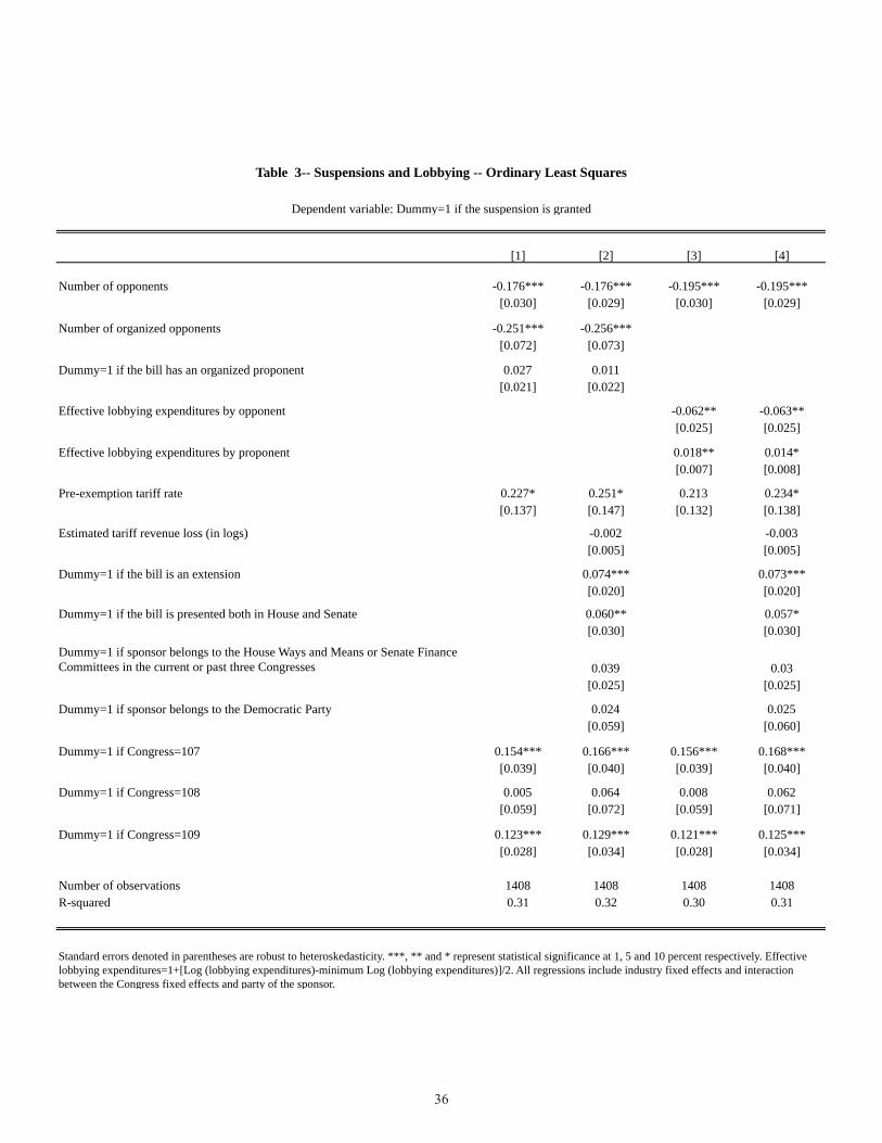
[1] [2] [3] [4]

Number of opponents -0.176*** -0.176*** -0.195*** -0.195***[0.030] [0.029] [0.030] [0.029]

Number of organized opponents -0.251*** -0.256***[0.072] [0.073]

Dummy=1 if the bill has an organized proponent 0.027 0.011[0.021] [0.022]

Effective lobbying expenditures by opponent -0.062** -0.063**[0.025] [0.025]

Effective lobbying expenditures by proponent 0.018** 0.014*[0.007] [0.008]

Pre-exemption tariff rate 0.227* 0.251* 0.213 0.234*[0.137] [0.147] [0.132] [0.138]

Estimated tariff revenue loss (in logs) -0.002 -0.003[0.005] [0.005]

Dummy=1 if the bill is an extension 0.074*** 0.073***[0.020] [0.020]

Dummy=1 if the bill is presented both in House and Senate 0.060** 0.057*[0.030] [0.030]

Dummy=1 if sponsor belongs to the House Ways and Means or Senate Finance Committees in the current or past three Congresses 0.039 0.03

[0.025] [0.025]

Dummy=1 if sponsor belongs to the Democratic Party 0.024 0.025[0.059] [0.060]

Dummy=1 if Congress=107 0.154*** 0.166*** 0.156*** 0.168***[0.039] [0.040] [0.039] [0.040]

Dummy=1 if Congress=108 0.005 0.064 0.008 0.062[0.059] [0.072] [0.059] [0.071]

Dummy=1 if Congress=109 0.123*** 0.129*** 0.121*** 0.125***[0.028] [0.034] [0.028] [0.034]

Number of observations 1408 1408 1408 1408R-squared 0.31 0.32 0.30 0.31

Table 3-- Suspensions and Lobbying -- Ordinary Least Squares

Standard errors denoted in parentheses are robust to heteroskedasticity. ***, ** and * represent statistical significance at 1, 5 and 10 percent respectively. Effective lobbying expenditures=1+[Log (lobbying expenditures)-minimum Log (lobbying expenditures)]/2. All regressions include industry fixed effects and interaction between the Congress fixed effects and party of the sponsor.

Dependent variable: Dummy=1 if the suspension is granted

36

[1] [2] [3] [4]

Number of opponents -0.130** -0.121** -0.138*** -0.133***[0.055] [0.055] [0.049] [0.049]

Number of organized opponents -0.283*** -0.292***[0.102] [0.101]

D=1 if bill has an organized proponent 0.063** 0.056*[0.028] [0.029]

Effective lobbying expenditures by opponent -0.064** -0.063**[0.031] [0.031]

Effective lobbying expenditures by proponent 0.041*** 0.040***[0.011] [0.011]

Pre-exemption tariff rate 0.264* 0.287** 0.257* 0.268*[0.143] [0.146] [0.138] [0.139]

Eestimated tariff revenue loss (in logs) -0.004 -0.006[0.005] [0.006]

Dummy=1 if the bill is an extension 0.077*** 0.077***[0.020] [0.021]

Dummy=1 if the bill is presented both in House and Senate 0.055* 0.049[0.030] [0.030]

Dummy=1 if sponsor belongs to the House Ways and Means or Senate Finance Committees in the current or past three Congresses 0.029 0.013

[0.025] [0.025]

Dummy=1 if sponsor belongs to the Democratic Party 0.035 0.044[0.060] [0.062]

Dummy=1 if Congress=107 0.169*** 0.184*** 0.180*** 0.198***[0.040] [0.041] [0.041] [0.041]

Dummy=1 if Congress=108 0.008 0.052 0.023 0.058[0.058] [0.070] [0.057] [0.068]

Dummy=1 if Congress=109 0.132*** 0.134*** 0.135*** 0.131***[0.028] [0.034] [0.028] [0.033]

Number of observations 1408 1408 1408 1408R-squared 0.22 0.23 0.20 0.21Instrumental variables

First-stage F (number of opponents) 24.56 25.53 20.16 21.1First-stage F (number of organized opponents) 30.95 27.90First-stage F (D=1 if bill has an organized proponent) 284.27 276.26First-stage F (effective lobbying expenditures by opponent) 32.46 33.03First-stage F (effective lobbying expenditures by proponent) 97.07 85.53Hansen's J statistic (p value) 0.44 0.38 0.75 0.63

Standard errors denoted in parentheses are robust to heteroskedasticity. ***, ** and * represent statistical significance at 1, 5 and 10 percent respectively. The first-stage regressions are shown in Table 5. The number of opponents; number of organized opponents; dummy for organized proponent; and the effective lobbying expendituresof opponents and proponents, are treated as endogenous. Effective lobbying expenditures=1+[Log (lobbying expenditures)-minimum Log (lobbying expenditures)]/2. All regressions include industry fixed effects and interaction between the Congress fixed effects and party of the sponsor.

Number of opponents who lobby on issues other than trade (or any other issue closely related to the bill)

Number of issues other than trade or any other issue closely related to the bill for which the opponent lobbies

Number of potential opponent firms that have expressed opposition in cuurent or past Congresses

Number of issues other than trade or any other issue closely related to the bill for which the proponent lobbies

Dummy =1 if proponent lobbies on issues other than trade (or any other issue closely related to the bill)

Number of potential opponent firms that have expressed opposition in cuurent or past Congresses

Table 4-- Suspensions and Lobbying --Instrumental Variables Regressions

Dependent variable: Dummy=1 if the suspension is granted

Number of potential opponent firms (in logs) Nnumber of potential opponent firms (in logs)

Number of potential opponents that are also currently proponents on bills on which the proponent is also contacted

Number of potential opponents that are also currently proponents on bills on which the proponent is also contacted

37

[1a] [1b] [1c] [2a] [2b] [2c] [3a] [3b] [3c] [4a] [4b] [4c]

Dependent variable: Number of opponents

Number of organized opponents

Dummy=1 if the bill has an

organized proponent

Number of opponents

Number of organized opponents

Dummy=1 if the bill has an

organized proponent

Number of opponents

Effective lobbying

expenditures by opponent

Effective lobbying

expenditures by proponent

Number of opponents

Effective lobbying

expenditures by opponent

Effective lobbying

expenditures by proponent

Number of contacted firms that are also currently proponents on bills on which the proponent is also contacted

-0.113*** -0.032*** -0.006 -0.127*** -0.034*** -0.012 -0.174*** -0.090*** 0.357*** -0.191*** -0.100*** 0.298***[0.027] [0.008] [0.015] [0.027] [0.009] [0.017] [0.031] [0.021] [0.079] [0.030] [0.022] [0.080]

Number of contacted firms that have expressed opposition in cuurent or past Congresses

0.082*** 0.012** -0.007 0.073*** 0.011** -0.012 0.100*** 0.043*** -0.167*** 0.095*** 0.042*** -0.179***[0.017] [0.005] [0.010] [0.017] [0.005] [0.010] [0.017] [0.016] [0.028] [0.017] [0.016] [0.028]

Number of potential opponent firms (in logs) 0.223*** 0.008 0.022** 0.231*** 0.009 0.029** 0.209*** -0.027 0.048 0.216*** -0.022 0.075*[0.032] [0.008] [0.011] [0.032] [0.008] [0.011] [0.032] [0.022] [0.043] [0.032] [0.023] [0.044]

Number of opponents which lobby on other issues 0.836*** 0.671*** -0.033 0.813*** 0.669*** -0.033[0.182] [0.111] [0.029] [0.181] [0.112] [0.028]

Dummy=1 if the bill has a proponent which lobbies on other issues 0 0.033*** 0.727*** -0.038 0.028*** 0.725***[0.037] [0.009] [0.020] [0.041] [0.010] [0.020]

Number of other issues for which the opponent lobbies 0.079*** 0.283*** -0.074*** 0.077*** 0.282*** -0.075***[0.026] [0.027] [0.015] [0.026] [0.027] [0.015]

Nnumber of other issues for which the proponent lobbies 0.012** 0.007 0.148*** 0.01 0.006 0.145***[0.006] [0.004] [0.009] [0.006] [0.004] [0.009]

Estimated tariff revenue loss (in logs) -0.42 0.326 -1.055*** -0.302 0.336 -0.983*** -0.421 1.151* -0.627 -0.347 1.193 -0.313[0.285] [0.206] [0.159] [0.318] [0.217] [0.162] [0.304] [0.696] [0.395] [0.339] [0.729] [0.423]

Pre-exemption tariff rate 0.013 -0.002 -0.008 0.016 0.008 0.030**[0.010] [0.002] [0.005] [0.010] [0.007] [0.015]

Dummy=1 if the bill is an extension -0.080** -0.014 0.060*** -0.091*** -0.027 0.157**[0.031] [0.009] [0.022] [0.033] [0.023] [0.063]

Dummy=1 if the bill is presented both in House and Senate 0.003 0.024* 0.098*** 0.013 0.082** 0.124[0.053] [0.014] [0.026] [0.054] [0.041] [0.079]

Dummy=1 if sponsor belongs to the House Ways and Means or Senate Finance Committees in the current or past three Congresses 0.112** 0.035** -0.037** 0.086 0.066* 0.076

[0.053] [0.014] [0.018] [0.054] [0.035] [0.068]Dummy=1 if sponsor belongs to the Democratic Party -0.017 0.027 -0.009 0.001 0.034 -0.256*

[0.072] [0.021] [0.048] [0.066] [0.072] [0.149]Dummy=1 if Congress=107 -0.118** -0.004 -0.069** -0.113** 0.007 -0.073** -0.167*** -0.074** -0.756*** -0.144*** -0.049 -0.897***

[0.046] [0.009] [0.028] [0.047] [0.012] [0.033] [0.051] [0.034] [0.094] [0.053] [0.035] [0.103]Dummy=1 if Congress=108 -0.101 0.023 -0.04 0.05 0.045 0.03 -0.066 0.127* -0.334*** 0.053 0.156* -0.350**

[0.073] [0.022] [0.032] [0.107] [0.032] [0.027] [0.076] [0.067] [0.125] [0.114] [0.091] [0.155]Dummy=1 if Congress=109 -0.226*** 0.007 0.021 -0.141** 0.027 0.050** -0.193*** 0.039 0.109 -0.103* 0.102*** 0.204**

[0.043] [0.013] [0.021] [0.058] [0.018] [0.024] [0.038] [0.029] [0.074] [0.053] [0.038] [0.087]

Number of observations 1408 1408 1408 1408 1408 1408 1408 1408 1408 1408 1408 1408R-squared 0.41 0.69 0.59 0.42 0.69 0.61 0.36 0.75 0.50 0.37 0.75 0.52

Table 5-- Suspensions and Lobbying --First Stage Instrumental Variables Regressions

Standard errors denoted in parentheses are robust to heteroskedasticity. ***, ** and * represent statistical significance at 1, 5 and 10 percent respectively. All regressions include industry fixed effects and interaction between the Congress fixed effects and party of the sponsor.

38

Number of opponents -0.181*** -0.181*** -0.184*** -0.183*** -0.097 -0.088 -0.126** -0.121**[0.032] [0.032] [0.032] [0.032] [0.066] [0.066] [0.053] [0.054]

Number of organized opponents (makes lobbying expenditures or PAC contributions) -0.199* -0.204*** -0.298*** -0.306***

[0.070] [0.072] [0.109] [0.108]Dummy=1 if the bill has an organized proponent (makes lobbying expenditures or PAC contributions) 0.021 -0.002 0.079** 0.072*

[0.024] [0.025] [0.035] [0.037]Effective lobbying expenditures and PAC contributions by opponent -0.047** -0.049** -0.055** -0.054**

[0.019] [0.019] [0.026] [0.026]Effective lobbying expenditures and PAC contributions by proponent 0.013* 0.008 0.042*** 0.042***

[0.007] [0.008] [0.011] [0.012]Pre-exemption tariff rate 0.204 0.225 0.243* 0.265* 0.387** 0.407** 0.326** 0.331**

[0.134] [0.140] [0.135] [0.144] [0.164] [0.170] [0.140] [0.142]Estimated tariff revenue loss (in logs) -0.002 -0.003 -0.004 -0.006

[0.005] [0.005] [0.005] [0.006]Additional controls No Yes No Yes No Yes No YesNumber of observations 1408 1408 1408 1408 1408 1408 1408 1408R-squared 0.30 0.31 0.30 0.31 0.21 0.22 0.20 0.21First-stage F (opponent) 24.56 25.53 20.16 21.1First-stage F (organized opponent) 27.01 26.80First-stage F (organized proponent) 153.30 151.86First-stage F (opponent lobbying expenditures) 35.23 36.04First-stage F (proponent lobbying expenditures) 73.30 63.55Hansen's J statistic (p value) 0.48 0.43 0.73 0.62

Dependent variable: Dummy=1 if the suspension is granted

OLS IV

Standard errors denoted in parentheses are robust to heteroskedasticity. ***, ** and * represent statistical significance at 1, 5 and 10 percent respectively. Dummies for whether the bill has an opponent; organized opponent and proponent; and their lobbying expenditures respectively, are treated as endogenous. All regressions include industry and Congress fixed effects, and interaction between the Congress fixed effects and party of the sponsor. The additional controls are the same as Table 4. All instruments are identical to Table 4.

Table 6 -- Suspensions and Lobbying --Broad Measure of Organization I (inlcuding campaign contributions by Political Action Committees)

39

Number of opponents -0.172*** -0.171*** -0.196*** -0.195*** -0.125** -0.118** -0.129** -0.125**[0.029] [0.029] [0.030] [0.030] [0.058] [0.057] [0.051] [0.051]

Number of organized opponent in current, past or future Congresses -0.243*** -0.252*** -0.292*** -0.305***[0.071] [0.070] [0.099] [0.097]

Dummy=1 if the bill has an organized proponent in current, past or future Congresses 0.01 -0.01 0.028 0.013[0.022] [0.023] [0.027] [0.028]

Effective lobbying expenditures by opponent in current, past and future Congresses -0.060** -0.062** -0.079** -0.080**[0.027] [0.027] [0.033] [0.034]

Effective lobbying expenditures by proponent in current, past and future Congresses 0.016** 0.011 0.050*** 0.050***[0.008] [0.008] [0.012] [0.013]

Pre-exemption tariff rate 0.243* 0.266* 0.219* 0.242* 0.287* 0.310** 0.307** 0.320**[0.139] [0.152] [0.132] [0.139] [0.148] [0.155] [0.142] [0.143]

Additional controls No Yes No Yes No Yes No YesNumber of observations 1408 1408 1408 1408 1408 1408 1408 1408R-squared 0.31 0.32 0.30 0.31 0.22 0.24 0.19 0.20First-stage F (opponent) 27.82 28.71 22.81 23.68First-stage F (organized opponent) 58.21 52.37First-stage F (organized proponent) 961.83 858.01First-stage F (opponent lobbying expenditures) 54.79 56.55First-stage F (proponent lobbying expenditures) 100.92 90.12Hansen's J statistic (p value) 0.26 0.20 0.91 0.84

Standard errors denoted in parentheses are robust to heteroskedasticity. ***, ** and * represent statistical significance at 1, 5 and 10 percent respectively. Effective lobbying expenditures=1+[Log (lobbying expenditures)-minimum Log (lobbying expenditures)]/2. The number of opponents; number of organized opponents; dummy for organized proponent; and the effective lobbying expendituresof opponents and proponents, are treated as endogenous. All regressions include industry and Congress fixed effects, and interaction between the Congress fixed effects and party of the sponsor. The additional controls are the same as Table 4. The instruments are the same as in Tables 4 and 6, except those for organization and effective lobbying expenditures, which are redefined to include past, current and future Congresses.

Table 7-- Suspensions and Lobbying --Broad Measure of Organization II (inlcuding lobbying in past and future Congresses)

Dependent variable: Dummy=1 if the suspension is grantedOLS IV

40

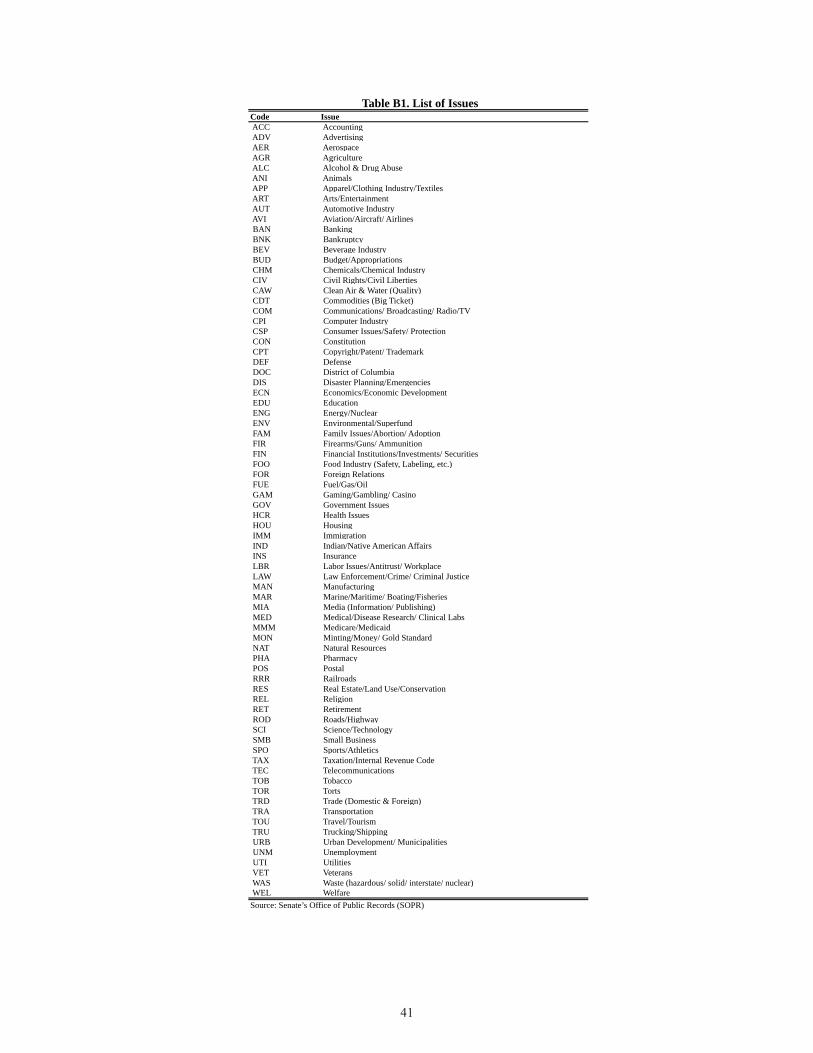
Code Issue

ACC Accounting ADV Advertising AER Aerospace AGR Agriculture ALC Alcohol & Drug Abuse ANI Animals APP Apparel/Clothing Industry/Textiles ART Arts/Entertainment AUT Automotive Industry AVI Aviation/Aircraft/ Airlines BAN Banking BNK Bankruptcy BEV Beverage Industry BUD Budget/Appropriations CHM Chemicals/Chemical Industry CIV Civil Rights/Civil Liberties CAW Clean Air & Water (Quality) CDT Commodities (Big Ticket) COM Communications/ Broadcasting/ Radio/TV CPI Computer Industry CSP Consumer Issues/Safety/ Protection CON Constitution CPT Copyright/Patent/ Trademark DEF Defense DOC District of Columbia DIS Disaster Planning/Emergencies ECN Economics/Economic Development EDU Education ENG Energy/Nuclear ENV Environmental/Superfund FAM Family Issues/Abortion/ Adoption FIR Firearms/Guns/ Ammunition FIN Financial Institutions/Investments/ Securities FOO Food Industry (Safety, Labeling, etc.) FOR Foreign Relations FUE Fuel/Gas/Oil GAM Gaming/Gambling/ Casino GOV Government Issues HCR Health Issues HOU Housing IMM Immigration IND Indian/Native American Affairs INS Insurance LBR Labor Issues/Antitrust/ Workplace LAW Law Enforcement/Crime/ Criminal Justice MAN Manufacturing MAR Marine/Maritime/ Boating/Fisheries MIA Media (Information/ Publishing) MED Medical/Disease Research/ Clinical Labs MMM Medicare/Medicaid MON Minting/Money/ Gold Standard NAT Natural Resources PHA Pharmacy POS Postal RRR Railroads RES Real Estate/Land Use/Conservation REL Religion RET Retirement ROD Roads/Highway SCI Science/Technology SMB Small Business SPO Sports/Athletics TAX Taxation/Internal Revenue Code TEC Telecommunications TOB Tobacco TOR Torts TRD Trade (Domestic & Foreign) TRA Transportation TOU Travel/Tourism TRU Trucking/Shipping URB Urban Development/ Municipalities UNM Unemployment UTI Utilities VET Veterans WAS Waste (hazardous/ solid/ interstate/ nuclear) WEL Welfare Source: Senate’s Office of Public Records (SOPR)

Table B1. List of Issues

41

Figure B1. Sample Bill Report

42

Figure B2. Sample Lobbying Report - 3M Company

43