protect a game theoretic system to protect the ports … · protect – a game theoretic system to...
TRANSCRIPT

PROTECT – A Game Theoretic
System to Protect the Ports of
United States
Milind Tambe, Bo An, Eric Shieh, Rong Yang
University of Southern California
November 9, 2011
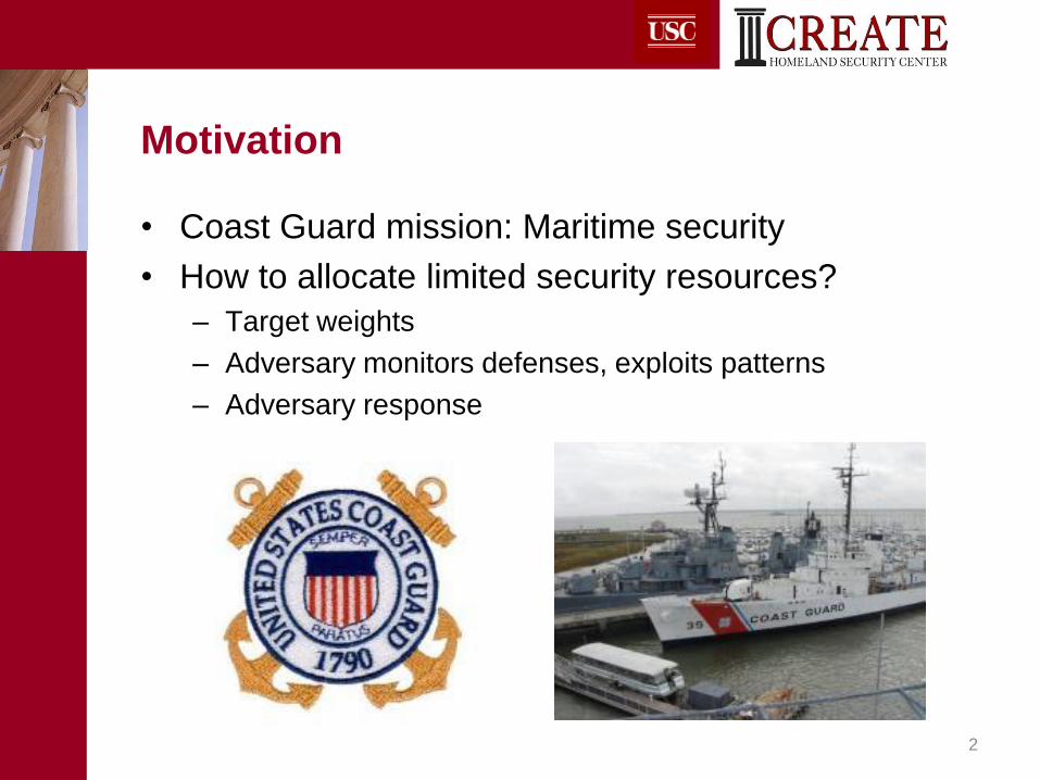
Motivation
• Coast Guard mission: Maritime security
• How to allocate limited security resources?
– Target weights
– Adversary monitors defenses, exploits patterns
– Adversary response
2

PROTECT: Randomized Patrols
3
Protect for US Coast Guard is being used at the port of Boston (below)

Contributions of PROTECT
• Previous security applications
• Key Contributions of PROTECT:
– 1st time Quantal Response Equilibrium (QRE) used in real world
– Compact representation of patrol schedules
– 1st time security application evaluated by Adversarial Perspective
Team (APT)
– 1st time with real data of patrols before/after 4
ARMOR: LAX IRIS: FAMS GUARDS: TSA
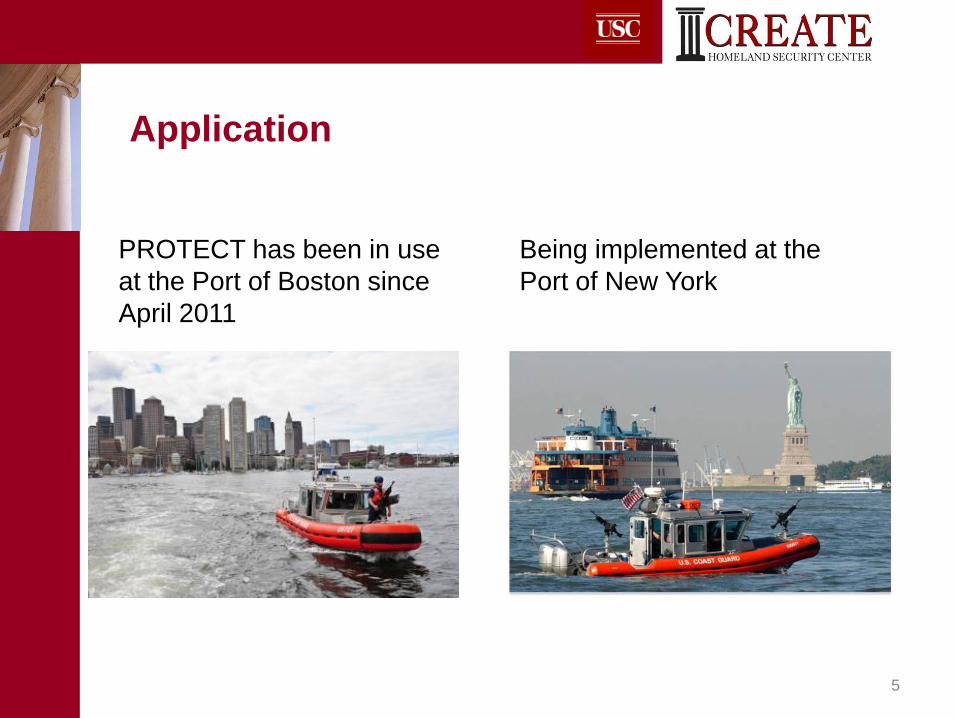
Application
5
PROTECT has been in use
at the Port of Boston since
April 2011
Being implemented at the
Port of New York

Outline
• PROTECT system
• Challenges
• Evaluation
• Future plan
6
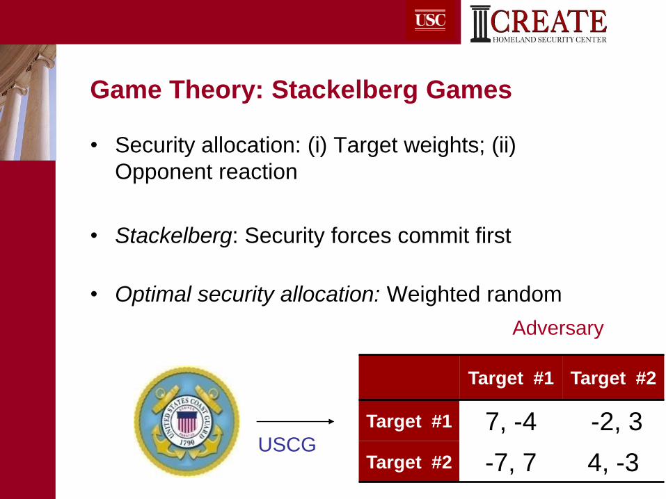
Game Theory: Stackelberg Games
7
• Security allocation: (i) Target weights; (ii)
Opponent reaction
• Stackelberg: Security forces commit first
• Optimal security allocation: Weighted random
Target #1 Target #2
Target #1 7, -4 -2, 3
Target #2 -7, 7 4, -3
Adversary
USCG

PROTECT System
• Casts the patrolling problem as a Stackelberg
game:
– Two players
• Defender actions (Coast Guard): Patrol routes
• Attacker actions(adversaries, terrorists): Attack targets
– Payoff matrix using defender & attacker actions
• Objective – Compute optimal strategy over
patrol routes to defend targets from attack
8

PROTECT System Overview
9
Game Matrix Attacker
Actions
Defender Actions:
Patrol Schedules
MSRAM
Target Data
Run PASAQ Sample over
Probabilities

Example for game matrix formulation
10
• Patrol # 2794: {1=T, 5=T, 6=T, 8=Q, 9=Q, 8=T, 6=T, 5=T,
1=T}
• Row of game matrix for defender; attacker’s matrix
opposite
• Columns correspond to target number
Target Number
Patrol Area 1 Patrol Area 2 Patrol Area 3 … Patrol Area 9
1 2 3 4 5 6 … 21
Patrol #: 2794 72.46 -8.22 -376.54 -54.56 -138.75 -50.83 … 578.21

PASAQ output - Probability Distribution
of Patrol Areas and Actions
11
Probability Patrol: Q = Query, O = Observe, T = Transit
0.05083 [(1:Q), (2:Q), (4:Q), (2:T), (1:T)]
0.05083 [(1:Q), (2:T), (4:Q), (2:Q), (1:T)]
0.05083 [(1:T), (2:Q), (1:Q), (2:T), (4:Q), (2:T), (1:T)]
0.05083 [(1:T), (2:Q), (4:Q), (2:T), (1:Q)]
0.05083 [(1:T), (2:T), (4:Q), (2:T), (1:Q), (2:Q), (1:T)]
0.05083 [(1:T), (2:T), (4:Q), (2:Q), (1:Q)]
0.00221 [(1:Q), (2:Q), (3:Q), (2:T), (4:Q), (2:T), (1:T)]
0.00221 [(1:Q), (2:Q), (4:Q), (2:T), (3:Q), (2:T), (1:T)]
0.00221 [(1:Q), (2:T), (3:Q), (2:Q), (4:Q), (2:T), (1:T)]
0.00221 [(1:Q), (2:T), (3:Q), (2:T), (4:Q), (2:Q), (1:T)]
0.00221 [(1:Q), (2:T), (4:Q), (2:Q), (3:Q), (2:T), (1:T)]
0.00221 [(1:Q), (2:T), (4:Q), (2:T), (3:Q), (2:Q), (1:T)]
0.00221 [(1:T), (2:Q), (1:Q), (2:T), (3:Q), (2:T), (4:Q), (2:T), (1:T)]
0.00221 [(1:T), (2:Q), (1:Q), (2:T), (4:Q), (2:T), (3:Q), (2:T), (1:T)]
… ….

Actionable Results: Schedule for 20 days
12
Day Hour: 0000 - 2300 Patrol: Q = Query, O = Observe, T = Transit
Day: 1 Hour: 1500 Patrol: [(1:T), (5:T), (6:T), (8:T), (9:Q), (8:Q), (6:T), (5:T), (1:T)]
Day: 2 Hour: 0300 Patrol: [(1:T), (5:T), (6:T), (8:T), (9:T), (8:T), (6:T), (5:T), (1:T), (2:T), (1:T)]
Day: 3 Hour: 1700 Patrol: [(1:T), (2:T), (4:Q), (2:T), (1:Q), (2:Q), (1:T)]
Day: 4 Hour: 1600 Patrol: [(1:T), (2:Q), (4:Q), (2:T), (1:Q)]
Day: 5 Hour: 1800 Patrol: [(1:T), (5:T), (6:T), (8:T), (9:Q), (8:T), (6:T), (5:Q), (1:T)]
Day: 6 Hour: 2300 Patrol: [(1:T), (5:T), (6:T), (8:T), (7:T), (5:T), (1:T), (2:T), (4:Q), (2:Q), (1:T)]
Day: 7 Hour: 0200 Patrol: [(1:T), (2:Q), (4:Q), (2:T), (1:Q)]
Day: 8 Hour: 1400 Patrol: [(1:T), (5:T), (6:T), (8:T), (9:Q), (8:T), (6:T), (5:Q), (1:T)]
Day: 9 Hour: 0600 Patrol: [(1:T), (5:T), (6:T), (8:Q), (9:Q), (8:T), (6:T), (5:T), (1:T)]
Day: 10 Hour: 1900 Patrol: [(1:T), (5:T), (6:T), (8:T), (9:Q), (8:T), (6:T), (5:Q), (1:T)]
Day: 11 Hour: 0600 Patrol: [(1:Q), (2:Q), (4:Q), (2:T), (1:T)]
Day: 12 Hour: 0000 Patrol: [(1:T), (2:T), (3:Q), (2:T), (4:Q), (2:Q), (1:Q)]
Day: 13 Hour: 1500 Patrol: [(1:T), (5:T), (7:T), (8:T), (6:T), (5:T), (1:T), (2:T), (4:Q), (2:Q), (1:T)]
Day: 14 Hour: 0200 Patrol: [(1:T), (2:T), (4:Q), (2:T), (1:Q), (2:Q), (1:T)]
Day: 15 Hour: 1400 Patrol: [(1:T), (5:Q), (6:T), (8:T), (9:Q), (8:T), (6:T), (5:T), (1:T)]
Day: 16 Hour: 0900 Patrol: [(1:Q), (2:Q), (4:Q), (2:T), (1:T)]
Day: 17 Hour: 2000 Patrol: [(1:T), (2:T), (4:Q), (2:T), (1:Q), (2:Q), (1:T)]
Day: 18 Hour: 1300 Patrol: [(1:T), (5:Q), (6:T), (8:T), (9:Q), (8:T), (6:T), (5:T), (1:T)]
Day: 19 Hour: 0700 Patrol: [(1:Q), (2:T), (4:Q), (2:Q), (1:T)]
Day: 20 Hour: 0800 Patrol: [(1:T), (5:Q), (6:T), (8:T), (9:Q), (8:T), (6:T), (5:T), (1:T)]

Outline
• PROTECT system
• Challenges
• Evaluation
• Future plan
13

Challenges
• Human Adversary
– Not assume perfectly rational attacker
• Scaling up
– # of possible schedules exponential
• Modeling CG domain
– Implementing real world
14

Human Adversary - QRE
• Game Theory and Human Behavior (IJCAI’11,
Yang et al.)
15
PT = Prospect theory
QRE = Quantal Response Equilibrium

QRE Background
• QRE in games (McKelvey et al, 1995; Weizsäcker,
2003; Yang et al, 2011)
• Model human attacker
• Humans choose better actions at higher frequency
• Noise added to decision/strategy
16
• qi = attacker probability
• U(x) = attacker’s expected utility for target x
• λ = noise in attacker’s strategy

PASAQ
• Piecewise-linear Approximation of optimal Strategy
Against Quantal response algorithm(PASAQ)
• PASAQ faster and provides higher quality strategy
17
Scaling Up
• Graph → Many paths
• Each vertex/patrol area of path has 3 possible
actions
• Example: Path of 5 patrol areas = 35 = 243 patrols
• Two Ideas
– Remove dominated patrols
– Combine similar patrols
18

Remove dominated patrols
• 3 Patrol Areas (1, 2, 3); 2 Defender Actions (A, B)
• Payoff(A) > Payoff(B)
19
Patrol # Patrol Schedule
1 (1,A), (2,A), (3,A), (2,B), (1,B)
2 (1,B), (2,A), (3,A), (2,B), (1,B)
3 (1,B), (2,B), (3,A), (2,B), (1,B)
• Patrols 2&3 - dominated
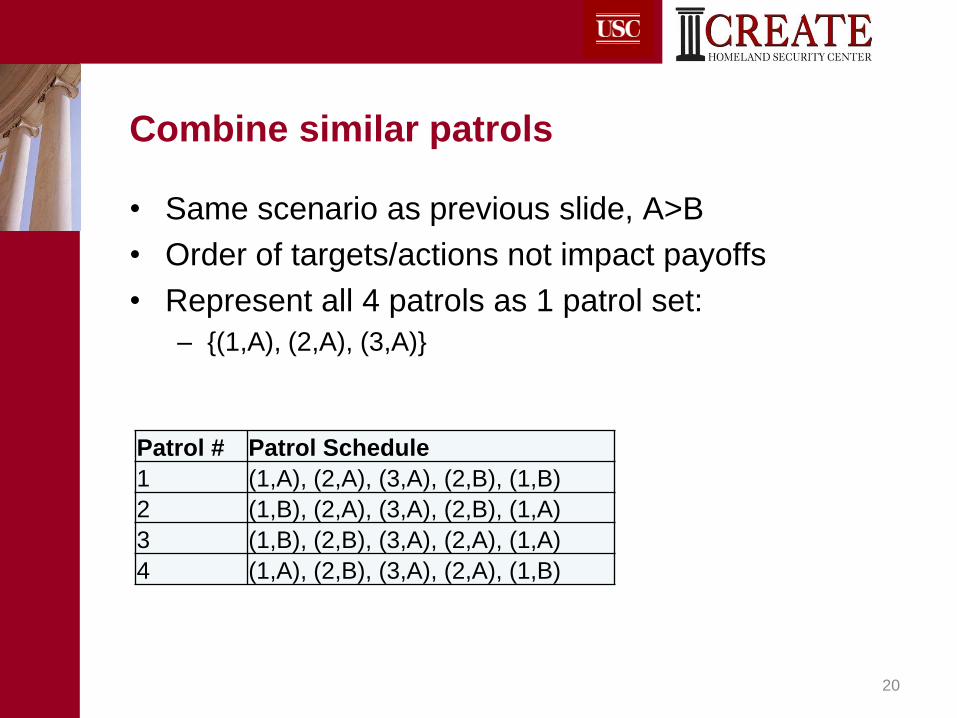
Combine similar patrols
• Same scenario as previous slide, A>B
• Order of targets/actions not impact payoffs
• Represent all 4 patrols as 1 patrol set:
– {(1,A), (2,A), (3,A)}
20
Patrol # Patrol Schedule
1 (1,A), (2,A), (3,A), (2,B), (1,B)
2 (1,B), (2,A), (3,A), (2,B), (1,A)
3 (1,B), (2,B), (3,A), (2,A), (1,A)
4 (1,A), (2,B), (3,A), (2,A), (1,B)

Comparison Full vs. Compact
21
0
100
200
300
400
500
600
60 70 80 90 100
Mem
ory
(M
B)
Max Patrol Time (minutes)
Full Compact
0
5
10
15
20
25
30
35
60 70 80 90
Ru
nti
me
(sec
on
ds)
Max Patrol Time (minutes)
Full Compact

Outline
• PROTECT system
• Challenges
• Evaluation
• Future plan
23

Evaluation
• Simulations in lab
• Expert feedback
• Adversarial team feedback
• Actual before/after data
24

Utility Analysis
25
-2
-1.5
-1
-0.5
0
0.5
0
0.5
1
1.5
2
2.5
3
3.5
4
4.5
5
5.5
6
Def
end
er E
xp
ecte
d U
tili
ty
Attacker λ value
PASAQ (λ=1.5)
DOBSS
Uniform Random
(Attacker)
Uniform Random
(Defender)

Robustness Analysis – Observation Noise
26
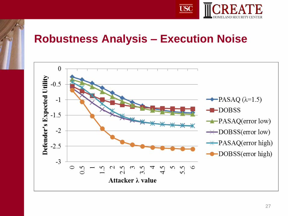
Robustness Analysis – Execution Noise
27
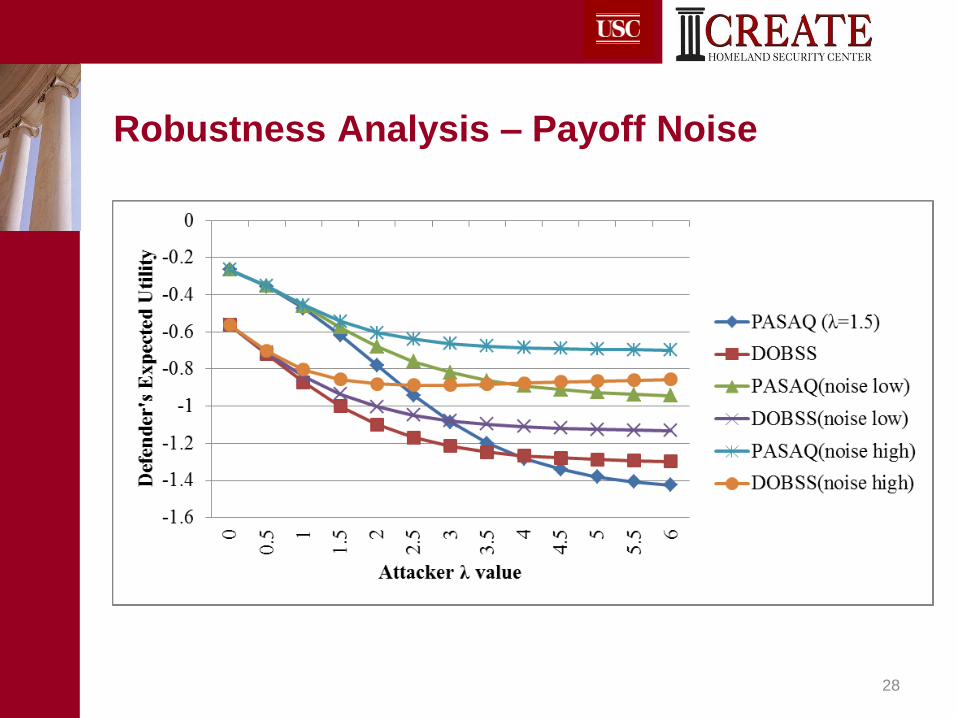
Robustness Analysis – Payoff Noise
28

Evaluation – Expert Feedback
29
• Commander, First Coast Guard District's
Operational Excellence Award for the work on
the PROTECT project
Evaluation – APT
• APT conducted a pre- and post-PROTECT
assessment
• Incorporate adversary’s known intent,
capabilities, skills, commitment, resources, and
cultural influences
• The effectiveness (in terms of tactical
deterrence) increased from the pre- to post-
PROTECT observations.
30

Evaluation – Pre-PROTECT
31

Evaluation – After PROTECT
32

Outline
• PROTECT system
• Challenges
• Evaluation
• Future plan
33
Future Work
• Move to New York
• Improved understanding of patrols and behavior
at patrol areas
• Include additional attack modes (i.e. Boat Bomb,
Swimmer/Diver/Underwater Delivery Systems,
Attack by Hijacked Vessel, Sabotage)
• Impact of patrols on deterrence
• Incorporate different assets (aerial)
• Impact of coordination/other gov’t agencies
34