Calhoun: The NPS Institutional Archive

Theses and Dissertations Thesis Collection

1991

Propulsion optimization for ABE, an Autonomous

Underwater Vehicle (AUV).

Woodford, Thomas James

Springfield, Virginia: Available from National Technical Information Service

http://hdl.handle.net/10945/28475

SSMsSS

hSKscscBWBfiWfKgi-'<-

EfiE BmSS Eft-•.'.••..-..

'"'•-.-"-•"-..-•...:- KCfij:-•-.:-

-"""•' :V'::^-'::-"~'

lUMtlMflmWITilMr^t iTi r*nT

Him

'''*'-'

KS ram i£BHKMHiflPSfli

•.-••»••-,

EVHB MMUlMWBftEHHS

IKS

JKjwMU

B90GI-"---';

BHBlHBSiBBi

HOMBntwp-

•

-

gBHBBKwffffnTlflWlPMVf CI WU flWi'^H'i* Ill'iVi

^fjfflr^WTwajip'riijiiTiiir 1

1

Mm

MBaS

Propulsion Optimization for ABE,

an Autonomous Underwater Vehicle (AUV)

by <'. 5L*

THOMAS JAMES .WOODFORD

B.S. Electrical Engineering

University of Virginia (1983)

Submitted in partial fulfillment of the

requirements for the degree of

MASTER OF SCIENCE IN OCEANOGRAPHIC ENGINEERING

at the

MASSACHUSETTS INSTITUTE OF TECHNOLOGY

and the

WOODS HOLE OCEANOGRAPHIC INSTITUTION

September 1991° Thomas J. Woodford, 1991

The author hereby grants to MIT and WHOI permission toreproduce and distribute copies of this thesis document in whole orin part. -.

Propulsion Optimization for ABE,an Autonomous Underwater Vehicle (AUV)

by

THOMAS JAMES WOODFORD

Submitted to the Massachusetts Institute of Technology/Woods Hole Oceanographic Institution

Joint Program in Oceanographic Engineeringon August 27, 1991 in partial fulfillment of the

requirements for the degree of

MASTER OF SCIENCE IN OCEANOGRAPHIC ENGINEERING

ABSTRACT

The oceanographic community is moving towards unmannedautonomous vehicles to gather data and monitor scientificsites. The mission duration of these vehicles is dependentprimarily on the power consumption of the propulsion system,the control system and the sensor packages

.

A customized propulsion thruster is designed. Thisincludes a specialized propeller tailored to ABE and a matchedmotor and transmission. A non-linear lumped parameter modelof the thruster is developed and experimentally verified. Themodel is used to predict thruster performance and compare thedesign thruster with other variants of propeller andmotor/transmission combinations.

The results showed that there is a trade-off betweenrapid dynamic response and power conservation. For thetypical ABE trajectory, the designed thruster provides gooddynamic response and the lowest power consumption of all themodelled thruster units.

Thesis Supervisor: Dr. Dana R. YoergerAssociate Scientist

Woods Hole Oceanographic Institution

Acknowledgements

The completion of this thesis was made possible by thesupport and encouragement of my friends and colleagues at theDeep Submergence Laboratory, who provided advice, help and aconstant reminder of reality.

Through the many trials and tribulations of preparing athesis (including hurricane Bob which wreaked havoc on theWoods Hole Oceanographic Institution on 19 August 1991 andleft the area without electrical power for nearly a week) I amespecially grateful to my wife Elizabeth. She stood by andprovided constructive criticism, proof reading service, andkept her good humor in spite of being forced to live the lifeof a gypsy as we moved between sources of power for mycomputer. For this invaluable service, I dedicate this paperto her.

The United States Navy is gratefully acknowledged for thegraduate education opportunity provided. This research wasalso supported by the National Science Foundation, grantnumber OCE 8820227.

Author's Biographical Note

LT Thomas J. Woodford, USN, completed his undergraduate

studies at the University of Virginia, receiving a Bachelor of

Science in Electrical Engineering and was commissioned in the

U.S. Navy in 1983. He completed nuclear propulsion and

Surface Warfare training in 1984 and was assigned to the USS

TRUXTUN (CGN-3 5) . On TRUXTUN he served as Damage Control

Assistant and Electrical Officer. He served as Shift Engineer

for the DIG prototype at the Nuclear Power Training Unit,

Ballston Spa, New York prior to his current assignment in the

Massachusetts Institute of Technology/ Woods Hole

Oceanographic Institution Joint Program in Oceanographic

Engineering

.

LT Woodford's next assignment, following completion of

his graduate studies, will be at the Surface Warfare Officer

School's Department Head Course in Newport, Rhode Island.

Following this school, he will be assigned as a Department

Head aboard a small combatant vessel of the U. S. Navy.

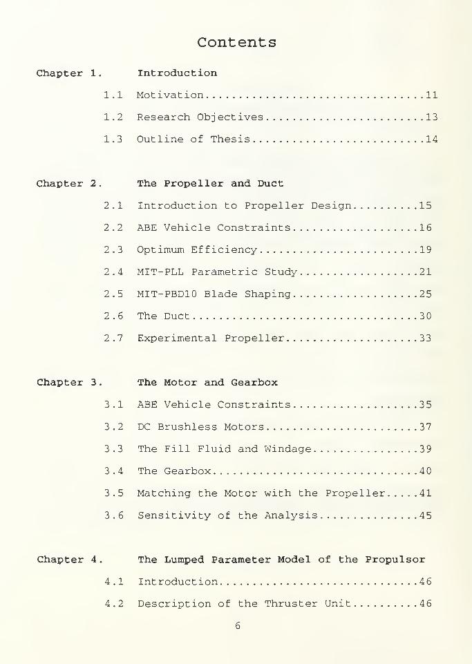
Contents

Chapter 1. Introduction

1 .

1

Motivation 11

1.2 Research Objectives 13

1 . 3 Outline of Thesis 14

Chapter 2. The Propeller and Duct

2 .

1

Introduction to Propeller Design 15

2.2 ABE Vehicle Constraints 16

2 . 3 Optimum Efficiency 19

2.4 MIT-PLL Parametric Study 21

2.5 MIT-PBD10 Blade Shaping 25

2 . 6 The Duct 3

2.7 Experimental Propeller 33

Chapter 3

.

The Motor and Gearbox

3.1 ABE Vehicle Constraints 35

3.2 DC Brushless Motors 37

3.3 The Fill Fluid and Windage 39

3 . 4 The Gearbox 4

3.5 Matching the Motor with the Propeller 41

3.6 Sensitivity of the Analysis 45

Chapter 4. The Lumped Parameter Model of the Propulsor

4 .

1

Introduction 46

4 . 2 Description of the Thruster Unit 46

6

4 . 3 The Complete Model 59

4.4 Simulation 62

4 . 5 Summary 63

Chapter 5. Experimental Verification

5 .

1

Experimental Setup 64

5 . 2 Steady State Response 66

5 . 3 Step Response 66

5 . 4 Sinusoidal Response 67

5 . 5 Summary 7 3

Chapter 6. Steady State Performance Comparison of Several

Thruster Units.

6.1 Introduction 75

6.2 ABE Thruster and the Other Thrusters 76

6 . 3 Steady State Comparison 80

6 . 4 Summary 84

Chapter 7. Balancing Dynamics and Efficiency

7 .

1

Introduction 8 5

7.2 Dynamic Comparison 88

7.3 An Open Loop Force Controller 89

7 . 4 Summary 97

Chapter 8. Summary, Conclusions, and Recommendations 9 9

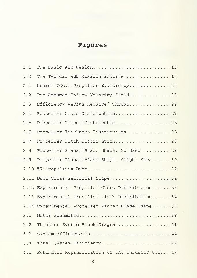
Figures

1 .

1

The Basic ABE Design 12

1.2 The Typical ABE Mission Profile 13

2.1 Kramer Ideal Propeller Efficiency 20

2 .2 The Assumed Inflow Velocity Field 22

2 . 3 Efficiency versus Required Thrust 24

2 . 4 Propeller Chord Distribution 27

2.5 Propeller Camber Distribution 28

2.6 Propeller Thickness Distribution 28

2.7 Propeller Pitch Distribution 29

2.8 Propeller Planar Blade Shape, No Skew 29

2.9 Propeller Planar Blade Shape, Slight Skew 30

2.10 5% Propulsive Duct 32

2.11 Duct Cross-sectional Shape 32

2.12 Experimental Propeller Chord Distribution 33

2.13 Experimental Propeller Pitch Distribution 34

2.14 Experimental Propeller Planar Blade Shape 34

3.1 Motor Schematic 38

3.2 Thruster System Block Diagram.. 41

3 . 3 System Efficiencies 44

3 .4 Total System Efficiency 44

4.1 Schematic Representation of the Thruster Unit... 47

8

4.2 Schematic Representation of the Propeller and Duct

Assembly 48

4.3 Bond Graph for the Propeller and Duct Assembly.. 54

4 . 4 Gearbox Schematic Diagram 55

4.5 Bond Graph for the Gearbox 56

4 . 6 The Motor Assembly 57

4 . 7 The Motor Bond Graph 58

4.8 The Complete Model Bond Graph 59

4 . 9 The Complete Model Block Diagram 61

4 . 10 The Simplified Block Diagram 62

5 . 1 The Experimental Test Stand 65

5 . 2 Model Step Response 66

5 . 3 Actual Thruster Step Response 67

5.4 Actual and Model Sinusoid Response, T=10 68

5.5 Actual and Model Sinusoid Response, T=5 69

5.6 Actual and Model Sinusoid Response, T=2.5 70

5.7 Actual and Model Sinusoid Response, T=1.25 71

5.8 Actual and Model Sinusoid Response, T=0.625 ....72

6 . 1 The Jason Propeller Response 78

6.2 The 18" Diameter, 6" Pitch Airplane Propeller

Response 79

6.3 The 18" Diameter, 8" Pitch Airplane Propeller

Response 80

6.4 The Experimental Propeller Response 81

6.5 Propeller Comparison, Torque Mode, MFM Motor.... 83

6.6 Propeller Comparison, Velocity Mode, MFM Motor.. 83

9

7 . 1 Simulation Tracks 87

7 . 2 Power Consumpt ion 9 5

7.3 Experimental Thruster Track #2, Velocity

Response 96

7.4 M88 Thruster Track #2, Velocity Response 96

7 . 5 Thruster Hover Response 97

10

Chapter 1

Introduction

1.1 Motivation

The Woods Hole Oceanographic Institution (WHOI) is

currently developing an autonomous underwater vehicle (ADV)

for scientific survey of the ocean floor. This vehicle has

been designated ABE, for the Autonomous Benthic Explorer.

As the oceanographic community explores the ocean floor,

the reliance on manned submarines to maintain ongoing

experiments has become restrictive. ALVIN, WHOI ' s manned

deep submersible, is unable to undertake new research, due to

an exhaustive schedule maintaining experiments that are

already in progress. ABE is being developed in order to free

up assets such as ALVIN and JASON, WHOI ' s unmanned

submersible, by performing routine data collection and

surveying at remote ocean bottom scientific sites.

Additionally, since ABE can operate without a nearby surface

ship operating as a tender/control ship, ABE will also free up

valuable research vessel time. In these respects, ABE will

complement the existing capabilities of tethered and manned submersibles.

11

ABE will be a long endurance vehicle with a typical

deployment of one year in length. This compares to an on-

station endurance of eight hours for a manned research

submersible (ALVIN) and around a month for tethered robots

(JASON) . During the deployment, ABE will observe a relatively

small area ( on the order of square kilometers ) of the ocean

floor at frequent intervals. Figures 1.1 and 1.2 show the

preliminary ABE configuration and a typical mission profile.

During a mission, ABE will remain in a semi-dormant state

for the majority of the time. At a predetermined interval or

in response to a trigger event, ABE will wake, and preform a

photographic survey along a preprogrammed flight path. Upon

completion of the survey, ABE will return to its mooring,

power down and wait for the next survey time.

- Black & WhiteCameras

Vertical Thrusters Glass Spheres

Thrusters

Strobes

Instrument &Battery Housing

Figure 1.1 The Basic ABE Design. [1]

12

In order for ABE to have sufficient battery power for a

one year mission, careful attention must be paid to developing

a highly efficient propulsion system. This research is

motivated by the need to develop this propulsion system.

(7) Deploy

{2j Glide until over target

AutonomousBenthic Explorer

• self powered• pre-programmed• long lite (1 year)

• can move 50 km at 1 knot

• carries films & CCD camera• carries CTD & transmissometer

• survey may be event triggered

Drop (5)descentweights

QQ Spiral down overct> bottom beacon

When 20m above (7) cp>bonom, move away _

"*~„ .

Perform regular stereo photo surveyol a pre-programmed region

Or survey region aroundanother area ot interest

Figure 1.2 The Typical ABE mission profilewill consist of four phases: Descent (1-6),Sleep (6), Survey (7-8), and Ascent. [1]

1.2 Research Objectives

There are two major components of a AUV propulsion

system. The first is the mechanical /hydrodynamic system

commonly referred to as a thruster or propulsor. The thruster

consists of an electric motor, a transmission and a

propeller/duct. The second component is the electronics and

the algorithm used to control the mechanical system.

13

The thruster must be optimized for the specific vehicle.

This involves designing a specialized propeller and duct

assembly then matching a suitable motor and gearbox to take

advantage of the motor's high speed efficiency and the

propeller's low speed efficiency. This is done to maximize

the conversion of electrical energy to thrust.

The control system must then be designed to provide the

best possible dynamic response, while taking advantage of the

mechanical system's most efficient operating conditions.

The objective of this research is to develop a propulsion

system that provides good dynamic response while maintaining

the high efficiency needed by ABE to perform its mission.

1.3 Outline of Thesis

Chapter 2 presents the design of an efficient propeller

for the ABE vehicle. Chapter 3 examines the selection of a

motor and gearbox matched to the ABE propeller. In Chapter 4,

a lumped parameter model of the thruster is developed.

Chapter 5 contains the experimental verification of the model.

Chapter 6 compares the steady state performance of the

designed ABE thruster with other thruster units. Chapter 7

examines the trade-offs that must be made between power

efficiency and beneficial dynamics. Chapter 8 summarizes the

results of the thesis and provides recommendations for further

research.

14

Chapter 2

The Propeller and Duct

The goal of this chapter is to develop a propeller and

duct combination for ABE that optimize the power conversion of

the thruster.

2.1 Introduction to Propeller Design

The propeller design presented here is based on the

Massachusetts Institute of Technology's (MIT's) propeller

development software. This software uses Lifting Line Theory

and optimum circulation to solve the complex hydrodynamics of

a marine propeller. [2]

The process used to design the propeller for ABE is as

follows

:

1. Calculate the drag of the tentative ABE

vehicle at the desired operating velocity.

2. Determine the thrust required.

3. Determine the physical constraints of the

vehicle that effect propeller size.

4. Estimate the wake field near the propeller.

15

5. Perform a parametric study using MIT's

Propeller Lifting Line program (MIT-PLL)

.

Minimize Power and torque for a given thrust.

6. Use MIT's Propeller Blade Design program

(MIT-PBD10) to calculate the blade shape from

MIT-PLL 's optimum output.

2.2 ABE Vehicle Constraints

2.2.1 ABE Physical Considerations

The ABE vehicle consists of two buoyancy pods supporting

a single instrument cylinder underneath. The buoyancy pods

are twenty one inch diameter series 58 bodies, and the

instrument cylinder is a twelve inch diameter streamline

cylinder. All three bodies are seven feet long and they are

connected by a series of struts. There are seven

thruster/propulsor units on ABE. Three are main propulsors

mounted at the stern of each cylinder. The remaining four are

thrusters for attitude and depth control. Two of these last

four thrusters are mounted vertically, and the other two are

mounted athwartships . ABE is designed to have a cruising

speed of one knot, and a minimum sprint capability of two

knots. The power budget allows 100 watts for normal

propulsion with a peak of 200 watts available. The propulsors

16

are limited to a diameter of eighteen inches by the space

available on ABE.

2.2.2 Vehicle Drag

The buoyancy pods are made up of twenty-one inch, series

58, streamlined shapes. Each pod will have a surface area of

28.1 ft 2. The drag on this type of body for relatively slow

speeds is primarily due to friction on the surface. The drag

can be calculated from the following equation:

Drag = ±pU2 CDS (2.1)

Where the drag coefficient, CD , is approximately equal to the

flat plate frictional drag coefficient, C F . For ABE at one

knot in seawater, the Reynold's Number is =6 X 10 5 and the

corresponding CF is <0.007.[3] S is the wetted surface area,

U is the velocity through the water, and p is the density of

the seawater. Using this equation, the drag of each of the

buoyancy pods at one knot is 0.56 lbf . The cylindrical

instrument case will be fitted with streamlined nose and tail

cones and equation (2.1) holds for this case as well. The

drag for the twelve inch diameter instrument case at one knot

is 0.44 lbf. The combined drag of the three main body

sections of ABE is 1.6 lbf.

17

Attention must be paid to the struts connecting the body

sections. Careful design of these structures can reduce

vehicle drag significantly. If it is assumed that the struts

are well designed and have a streamlined cross-section, then

equation 2.1 above can be used to calculate the drag. The

term S is now equal to the entire wetted surface of the strut

(top and bottom surfaces) . Assuming nine feet of struts with

one inch maximum thickness and five inches width, the

calculated drag is =0.15 lbf

.

However, if the struts are poorly designed the drag

increases by an order of magnitude. Assuming a 1-inch

circular cross-section, the drag is now calculated by:

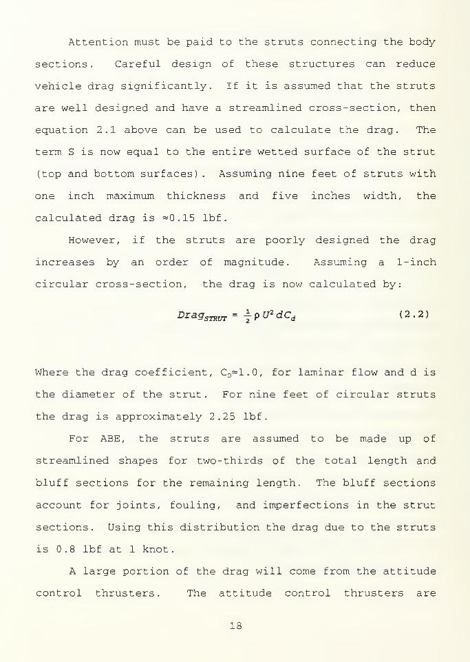
DragSTRUT = ±pU2 dCd (2.2)

Where the drag coefficient, C D=1.0, for laminar flow and d is

the diameter of the strut. For nine feet of circular struts

the drag is approximately 2.25 lbf.

For ABE, the struts are assumed to be made up of

streamlined shapes for two-thirds of the total length and

bluff sections for the remaining length. The bluff sections

account for joints, fouling, and imperfections in the strut

sections. Using this distribution the drag due to the struts

is 0.8 lbf at 1 knot.

A large portion of the drag will come from the attitude

control thrusters. The attitude control thrusters are

comprised of four thrusters mounted perpendicular to the flow

streamlines when ABE is traveling in the forward direction.

These thrusters will be used to make minor corrections to the

vehicle's depth and heading. These thrusters will be ducted

to prevent fouling and impact damage. Each unit will have a

3 inch diameter, streamlined motor case and a 3 inch by 18

inch duct that will be streamlined for forward motion. Using

the above equations, each thruster will have a drag of 0.2

lbf .

The total vehicle drag for a forward speed of 1 knot is

3.2 lbf. For the purposes of propeller design, each thruster

will be designed to give 3 lbf at 1 knot. This allows ABE to

maintain a full speed capability in the event of the failure

of one of the three main propulsion thrusters. Additionally,

ABE will have an excess propulsive force available during

normal cruising conditions.

2.3 Optimum Efficiency

Using the thrust of 3 lbf determined from the drag, the

vehicle's speed of one knot, an estimated shaft speed of 100

rpm, and the 1.5 foot propeller diameter, the ideal efficiency

can be determined from the Kramer diagram, Figure 2.1 [2].

The entering arguments for the diagram are X (a form of the

ship advance coefficient, Js ) and C T , the thrust coefficient.

19

For ABE these coefficients are

71

S _1.6 87 8 -£-

sec

mid % (lOOrpzn) (-—-2*2.) (l.sft)6 sec

= 0.22(2.3)

Cr - 3ijbf

4-pTCV^i? 2 in (1.9905^^-) (1.687 8-^ )2

( .7 5ft)= 0.60

0007 0004 001 002 004 0.1 2 01Absolutt Advance Coefficient X -

I IS Z 343680

Figure 2.1 Kramer Ideal Propeller Efficiency[2]

20

The ideal efficiency for a three blade propeller

operating under these conditions is ^^83%. [2] This

represents the maximum efficiency possible, neglecting viscous

forces

.

2.4 A Parametric Study using MIT-PLL

Using the information already discussed, we are almost

ready to begin using MIT-PLL to start developing some chord

and thickness distributions for the ABE propeller blade. In

order to enter MIT-PLL, initial chord and thickness

distributions must be assumed and a inflow velocity field

needs to be determined.

The initial chord and thickness distribution were assumed

to be linear. At the hub, the chord is 2 inches, the

thickness is Vi inch. At the blade tip, the chord is lA inch

with a tenth of an inch thickness.

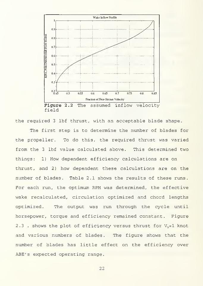
For an accurate inflow field to be determined, extensive

model testing must be performed. Since this type of testing

is beyond the scope of this paper, a simple inflow field is

assumed. This field is shown in Figure 2.2.

With this information, a parametric study of several

potential propellers was conducted. The parameters used in

this study are: (1) Number of Blades, (2) RPM, and (3) Blade

Shape (in a qualitative sense) . The goal is to find the

maximum efficiency and the minimum power required to generate

21

1

0.9

t 0.8as

o5 0.7

%a

| 0.6e3

oZ

£ 0.4

0.3

0.20.

Wake Inflow Profile

45 0.5 0.55 0.6 0.65 0.7 0.75 0.8 0.85

Fraction of Free-Stream Velocity

Figure 2.2 The assumed inflow velocityfield

the required 3 lbf thrust, with an acceptable blade shape.

The first step is to determine the number of blades for

the propeller. To do this, the required thrust was varied

from the 3 lbf value calculated above. This determined two

things: 1) How dependent efficiency calculations are on

thrust, and 2) how dependent these calculations are on the

number of blades. Table 2.1 shows the results of these runs.

For each run, the optimum RPM was determined, the effective

wake recalculated, circulation optimized and chord lengths

optimized. The output was run through the cycle until

horsepower, torque and efficiency remained constant. Figure

2.3 . shows the plot of efficiency versus thrust for Vs =l knot

and various numbers of blades. The figure shows that the

number of blades has little effect on the efficiency over

ABE's expected operating range.

22

Thrust—

»

Bid: 3

0.5

lbf

1.0

lbf

2.0

lbf

3.0

lbf

4.0

lbf

5.0

lbf

8.0

lbf

10.0

lbf

HP .001 .003 .006 .010 .014 .018 .033 .044

Torque .14 .23 .39 .54 .68 .82 1.22 1.48

RPM 45.5 58.7 77.9 92.8 105 115 142 157

Tl .875 .819 .749 .702 .666 .637 .573 .542

Blades

:

4

HP .001 .003 .006 .009 .014 .018 .033 .044

Torque .15 .26 .43 .60 .75 .91 1.35 1.63

RPM 41.3 53.1 70.1 83.1 94.4 104 128 141

Tl .875 .820 .751 .704 .668 .639 .576 .544

Blades

:

5

HP .001 .003 .006 .009 .014 .018 .033 .044

Torque .16 .28 .47 .65 .81 .97 1.44 1.75

RPM 38.9 48.2 65.2 77.2 87.7 96.9 119 131

Tl .872 .818 .75 .704 .669 .640 .576 .545

Table 2 . 1 (No Tunnel Used in Calculations

23

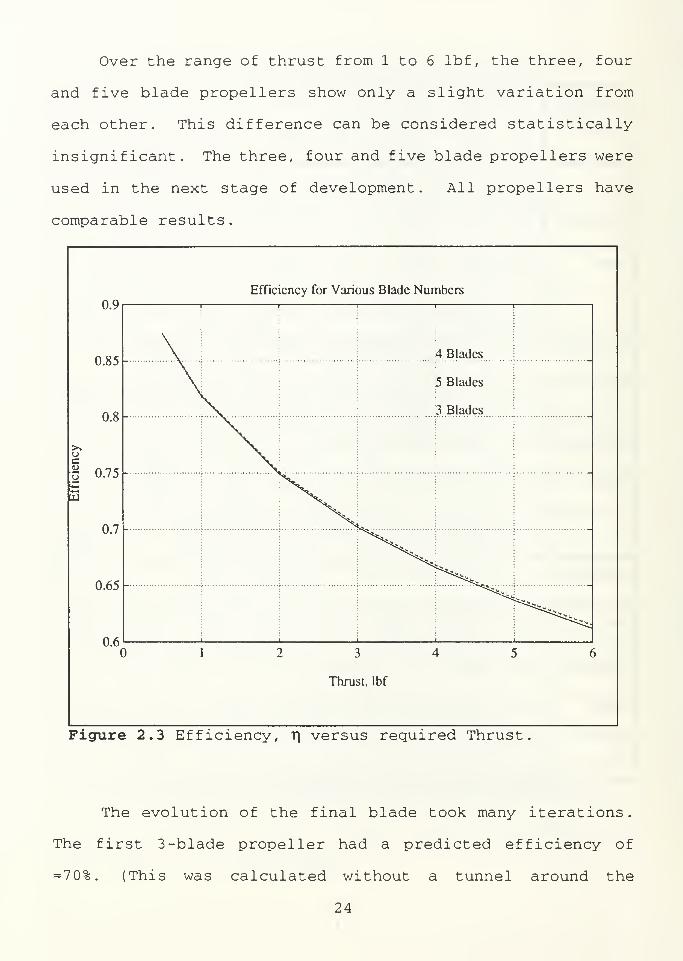
Over the range of thrust from 1 to 6 lbf, the three, four

and five blade propellers show only a slight variation from

each other. This difference can be considered statistically-

insignificant. The three, four and five blade propellers were

used in the next stage of development. All propellers have

comparable results.

0.9

0.85

0.8

o

I 0.75

UJ

0.7

0.65

0.6

Efficiency for Various Blade Numbers1 1

_1

4 Blades

5 Blades

3 Blades

^%>

<<^IcItIt

Thrust, lbf

Figure 2.3 Efficiency, T) versus required Thrust

The evolution of the final blade took many iterations.

The first 3-blade propeller had a predicted efficiency of

=70%. (This was calculated without a tunnel around the

24

propeller.) The resulting chord distribution had an extremely

narrow blade with a very sharp tip. This blade was not

physically suited for use in the marine environment. Any

fouling or impact with an obstruction (eg. fish) would have

destroyed the blade.

Several chord distributions were used. By taking the

output of one run, the planer blade shape was plotted (based

on the chord distribution). From this plot, a new, more

rugged chord distribution was developed. This chord

distribution was used for the next MIT-PLL run as the initial

blade input. For each run of MIT-PLL, the thrust (3 lbf), the

diameter (1.5 ft) and the inflow velocity field were held

constant. The RPM, circulation, and chord lengths were

optimized. After several iterations, a final 3-blade

propeller with a 66.1% efficiency and a 4-blade propeller with

a 66.4% efficiency were chosen. These propellers showed the

highest efficiency, with durable blade dimensions.

The three blade propeller is presented since a

commercially available propeller similar to the designed

propeller was readily obtained. The commercial propeller is

presented in section 2.7 .

2.5 MIT-PBD10, Blade Shaping

After using MIT-PLL to determine the desired circulation,

chord and thickness distributions, the actual blade shape and

25

camber that will develop the desired circulation must be

calculated. The code used for this is MIT's Propeller Blade

Design program, PBD10. To enter MIT-PBD10, a rake and skew of

the blade is required in addition to the MIT-PLL output.

Since rake has negligible effects and serves no purpose for

the ABE vehicle, no rake is used. The primary purpose of skew

is to balance (by phase shift) unsteady forces on the

propeller. Since the forces on ABE are small and the speeds

of operation are low, the unsteady forces are neglected and a

small amount of skew (8° at the tip) was added to aid in

obstruction shedding.

The recommended default values for MIT-PBD10 were used

initially. These values determine the nature and extent of

the wake field. The two dimensional blade cross-section shape

was chosen as a NACA a=0.8 mean line. Slight modifications

were made to the extent and contraction of the wake field in

order for PBD10 to run smoothly in this particular case. The

PBD10 output for Kj., Kg and the induced velocities are similar

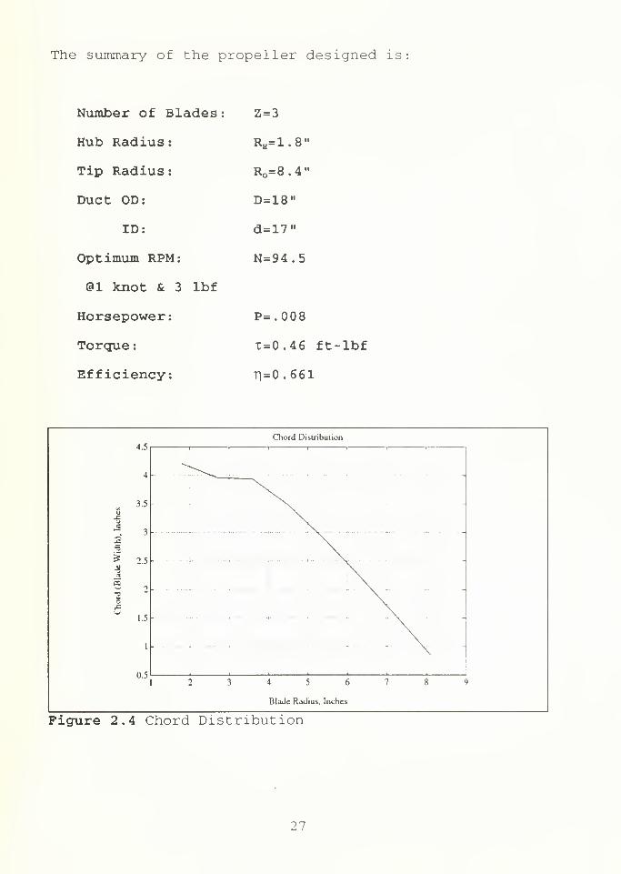
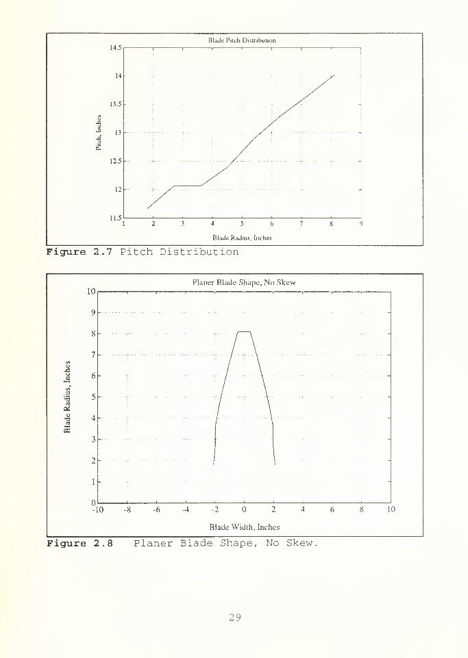
to what was described by PLL. Figures 2.4 through 2.7 show

the resulting blade shape determined by the above process.

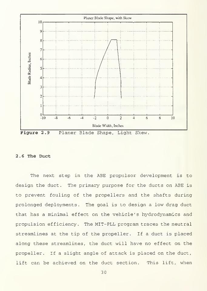
Figures 2.8 and 2.9 show a planer view of the blade, with and

without skew.

26

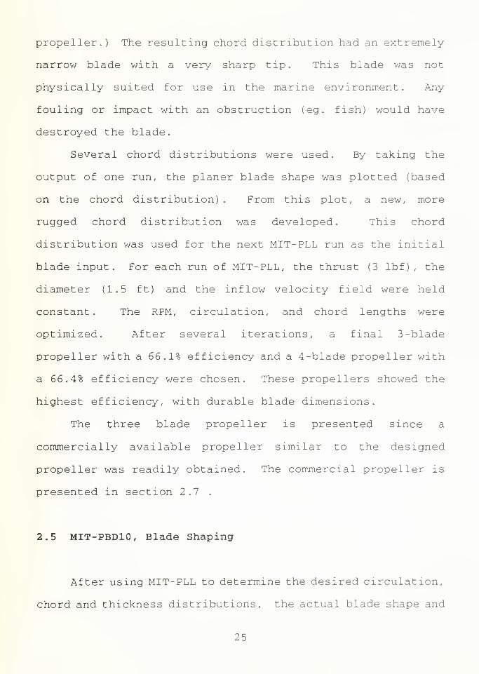
The summary of the propeller designed is

Number of Blades

:

Hub Radius

:

Tip Radius

:

Duct OD:

ID:

Optimum RPM:

@1 knot & 3 lbf

Horsepower:

Torque

:

Efficiency:

Z=3

RH=1.8"

R =8.4"

D=18"

d=17"

N=94.5

P=.008

X=0.46 ft-lbf

Tl = 0.661

4.5

4

3.5

OJZ

* 3

* 2.5

a«

1 2

6,,

1

0.5

Chord Distribution

"TK[\i

\ -

\2 3 4 5 6 7 8

Blade Radius, Inches

>

Figure 2.4 Chord Distribution

27

Camber (Fo/C) Distribution

0.06

0.055 -

0.05

•«j 0.045

0.04

0.035

0.034 5 6

Blade Radius. Inches

Figure 2.5 Camber Distribution

Blade Thickness Distribution

0.6

0.55

0.5

- 0.45

|S 0.4

£ 0.35

0.3

0.25

0.2

0.15

0.1

i

1 4 5 6

Blade Radius. Inches

Figure 2.6 Thickness Distribution

28

Blade Pitch Distribution

14.5

13.5

13

12.5

12

11.54 5 6 7

Blade Radius. Inches

Figure 2.7 Pitch Distribution

10

9

8

7t«u-e

46

1 5

as

•8 4

s3

2

1

-1

Planer Blade Shape, No Skew

,

,

r 1

0-8-6-4-2 2 4 6 8 1

Blade Width, Inches

Figure 2.8 Planer Blade Shape, No Skew.

2 9

10

9

8

7

Oi

J 6

i 5

as

8 4

s3

2

1

-1

Planer Blade Shape, with Skew

0-8-6-4-2 2 4 6 8 10

Blade Width, Inches

Figure 2.9 Planer Blade Shape, Light Skew,

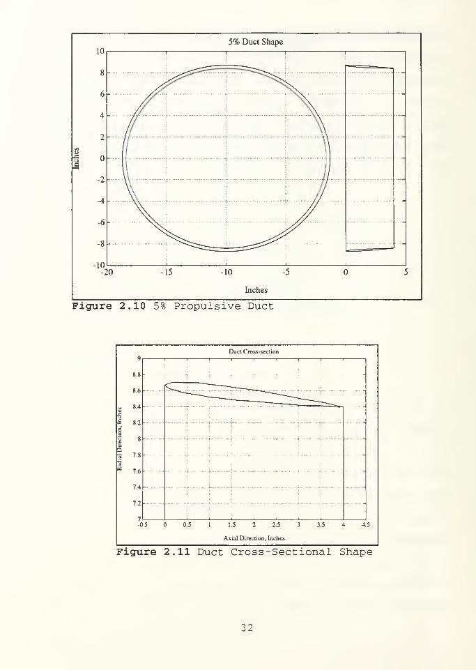
2.6 The Duct

The next step in the ABE propulsor development is to

design the duct. The primary purpose for the ducts on ABE is

to prevent fouling of the propellers and the shafts during

prolonged deployments. The goal is to design a low drag duct

that has a minimal effect on the vehicle's hydrodynamics and

propulsion efficiency. The MIT-PLL program traces the neutral

streamlines at the tip of the propeller. If a duct is placed

along these streamlines, the duct will have no effect on the

propeller. If a slight angle of attack is placed on the duct,

lift can be achieved on the duct section. This lift, when

30

summed around the entire duct, becomes a propulsive force (as

opposed to drag) . Using MIT-PLL, a duct with a slight

propulsive force was designed. The neutral nose-tail angle of

attack is 4.4 degrees. The angle of attack for 5% duct

propulsion is 3.8 degrees. The cross-sectional shape for the

duct is the NACA 0008 Basic thickness form. [4] Figures 2.10

and 2.11 show this duct.

31

5% Duct Shape

10

8

6

4

2

a

-2

-4

-6

-8

-10

^--—,—:>*^-^>^

,^

.0 -15 -io -5 o :

Inches

Figure 2.10 5% Propulsive Duct

9

8.8

8.6

8.4It

-Cu5 8.2

eo5 8w

5« 7.83a

7.6

7.4

7.2

7-0

Duct Cross-section!!!!'!!!>c^ -——~____^

"1 i———HHHr—~^^

.5 0.5 1 1.5 2 2.5 3 3.5 4 4

Axial Direction, Inches

5

Figure 2.11 Duct Cross-Sectional Shape

32

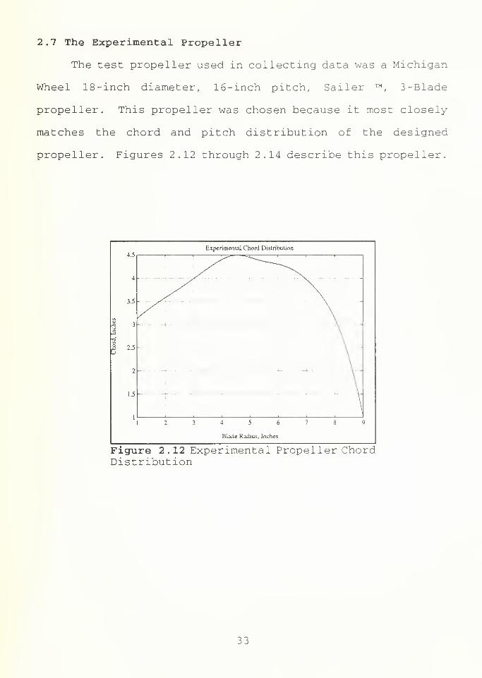
2.7 The Experimental Propeller

The test propeller used in collecting data was a Michigan

Wheel 18-inch diameter, 16-inch pitch, Sailer ™, 3-Blade

propeller. This propeller was chosen because it most closely

matches the chord and pitch distribution of the designed

propeller. Figures 2.12 through 2.14 describe this propeller.

4.5

4

3.5

3

:.5

2

1.5

i

Experimental Chord Distribution

1

i

,

.

i

i

4 5 6

Blade Radius, Inches

Figure 2.12 Experimental Propeller Chore.Distribution

33

18

17

16

ux:

A 15

3£

14

13

12

Experimental Blade!!':'""i ! j

2 3 4 5 6 7 8 9

Blade Radius, Inches

Figure 2.13 Experimental Propeller PitchDistribution

10

9

8

7c/l

U

a 6

1 5

aS"J AT3 4«J

3

2

1

-]

Experimental Blade

:

\1 1

1

l\ 1

i0-8-6-4-2 2 4 6 8 1

Blade Width, Inches

Figure 2.14 Experimental Propeller Planer Blade Shape

34

Chapter 3

The Motor and Gearbox

3.1 ABE Vehicle Constraints

There are several serious constraints placed on the

mechanical design of the motor and transmission by ABE's

mission environment. The two primary considerations are the

ambient pressure of the ocean bottom and the limited supply of

electrical power provided by onboard batteries.

In order to survive the extreme pressure (10,000 psi),

the motor assembly must either be pressure tolerant or

isolated from the pressure. In order to isolate the motor, a

heavy pressure vessel must be constructed and the motor sealed

inside. There must be a shaft seal around the output shaft.

This seal must be leak proof at an extremely large

differential pressure. Such a seal is expensive and produces

a large added load on the motor. This load reduces system

efficiency in a dramatic way. Pressure tolerant motors also

require shaft seals. However, since the internal pressure of

the motor casing is maintained at a few pounds above ambient

35

pressure, the differential pressure (DP) is very low. For low

DPs, the added load is very low. Additionally, seals that

operate with high differential pressure are prone to slight

leakage. Any leakage of seawater over an extended period of

time can result in failure of electric devices. For these

reasons, shaft seals with high differential pressure should be

avoided in this application, and a pressure tolerant motor

should be used.

The disadvantage of the pressure tolerant motor is an

increased loss of power due to windage. The windage comes

from the fluidic drag on the rotor of the motor due to the

presence of a fill fluid. The fill fluid is a non-conductive

fluid maintained at a few psi above ambient pressure and it

surrounds and fills the motor. This prevents the highly

conductive and corrosive seawater from entering the motor.

Since ABE is a battery powered vehicle with a bus voltage

of 48 VDC, a DC motor is the obvious choice for the prime

mover of the thruster.

The transmission must be selected to match the motor,

which is most efficient at high speeds, to the propeller,

which has high efficiency at lower speeds. The gearbox must

also be of sufficiently high quality and precision to minimize

the losses due to the gearing.

36

3.2 DC Brushless Motors

3.2.1 Brushed versus Brushless Motors

DC motors come in two main types: Brushed and Brushless.

Brushed motors are the most common DC motor. They have a

mechanical arrangement of split rings and brushes called a

commutator. The commutator switches the voltage applied to

the coils depending on the position of the rotor. This

switching keeps a positive force on the rotor to keep it

rotating. A brushless motor relies on electronics to provide

the proper commutation to the motor based on feedback from an

external rotor position detector.

In a high pressure environment, spring loaded brushes

experience increased wear and a tendency to hydroplane on the

non-conductive fill fluid. The hydro-planing leads to brush

chatter and an increased heat load due to the increased

electrical resistance. Brushed motors have a short life

expectancy in the high pressure environments.

Since the commutation on brushless motors is accomplished

electronically, they do not suffer from any of the above

problems. They are, however, much more expensive and require

complicated (and expensive) controllers. Due to the

importance of longevity and reliability in ABE's mission

environment, DC brushless motors will be used.

37

3.2.2 Motor Equations

In order to evaluate the motor, the efficiency of the

motor is calculated. The motor chosen for ABE is a Pittman

elcom © 5100 series DC brushless motor. This motor was chosen

for size and rated capacity. A schematic of the motor,

defining the variables used in the equations, is shown in

Figure 3.1 .

R

Controller Vs back

Motor

Supply

TauM

^J Omega M

Figure 3.1 Motor Schematic

The motor constants and parameters for this motor are

Torque Constant: KT = 0.173 Nm/Amp

Back EMF Constant: KE = 0.173 V/(rad/sec)

Coil Resistance: Rc = 4.85 ohms [5]

38

For steady state operation, the following equations describe

the operation of a DC motor:

Back EMF: VBACK = KE CO^

Motor Torque: x m = KT I m

Motor Current: Im = ( Vs- VBACK ) /Rc

Where Vs is the supply voltage and co^ is the angular velocity

of the rotor. Efficiency can be calculated as:

t, = Ism = J^£ (3.D" Pin VaIa

From equation 3.1, it can be seen that efficiency

increases with motor speed. This neglects the effect of

windage which increase with speed.

3.3 The Fill Fluid and Windage

The fluid used for compensation is Halocarbon © 0.8 cSt

fluid. This is a silicon oil based fluid with a viscosity 20%

less than water. Of the commercially available, non-

conductive fluids, this fluid provides pressure compensation

and has the lowest viscosity. For the purposes of efficiency

calculation, the fluid flow around the rotor will be

considered to be laminar flow between two parallel surfaces.

From testing of other motors with this fluid, a linear

relationship exists between torque due to drag and angular

velocity. The proportionality constant in this relationship

39

is K„ = 5.175 x 10" 5 Nm/(rad/sec) . The torque lost (xj and the

power lost (Pw ) due to windage are: [6]

x w = Kw (»ia and Pw = Kw<*>2m

3 . 4 The Gearbox

Gearboxes are available in a wide variety of types, gear-

ratios and efficiency. Gearbox efficiency is highly dependent

on the manufacturer's tolerances and construction procedures.

For the Pittman motors, a variety of planetary gearboxes are

available. These gearboxes will be used to determine the

desired gear ratio for the ABE thruster. In order to

calculate the desired gear ratio, descriptive equations of the

performance of the gearbox must be determined. The equations

must be written in terms of gear ratio.

To formulate the equations it is assumed that a planetary

gearbox is made up of an arbitrarily small stage. A certain

number of these stages are stacked in order to get the desired

reduction ratio. Each stage has a specific gear reduction

(1.1:1) and a specific efficiency (T^) . The complete gearbox

then has a gear reduction ratio of (1.1) n :l and an efficiency

of Thn where n is the number of stages (including fractional

stages) needed to get the desired reduction. For the Pittman

gearboxes, two advertised gearboxes are a 4:1 and a 17.33:1

gear ratio with efficiencies of 80% and 64% respectively. If

the 4:1 gearbox is used as a baseline, n=14.545 and 1^ = 0.985.

40

If these numbers are used to calculate the efficiency for the

17.33:1 gearbox, n=29.93 and the efficiency is 63%. Since

this is a good match, the following equations will be used to

describe the gearbox:

N = (1.1) AND T) G = (0.985)" (3.3)

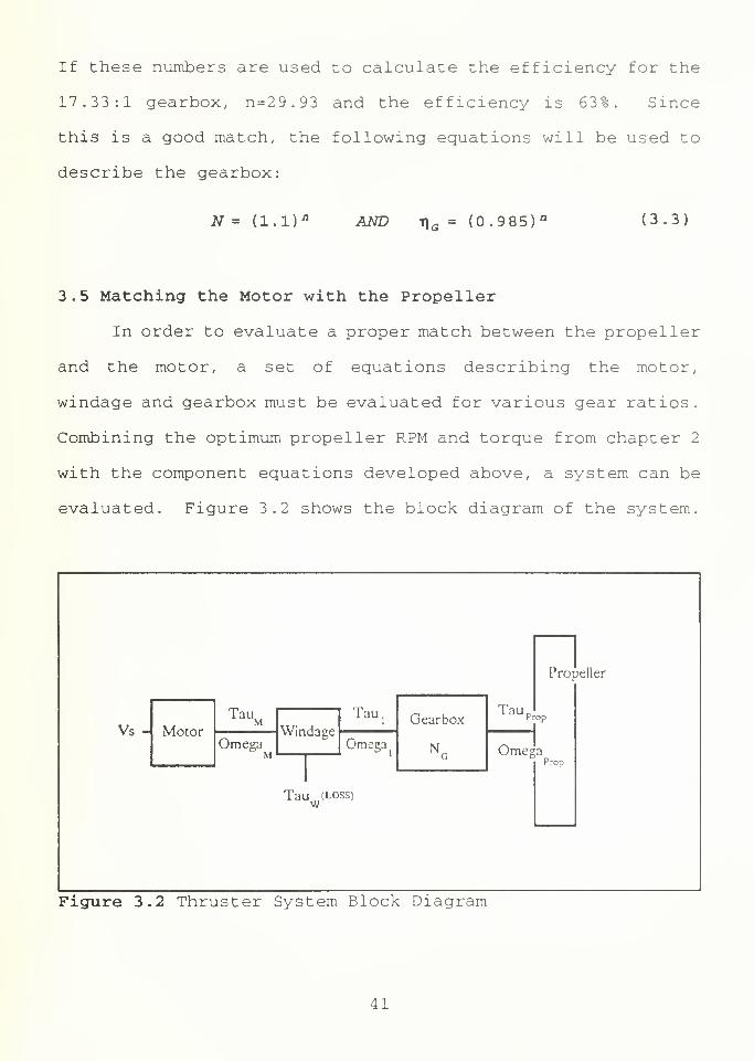
3.5 Matching the Motor with the Propeller

In order to evaluate a proper match between the propeller

and the motor, a set of equations describing the motor,

windage and gearbox must be evaluated for various gear ratios.

Combining the optimum propeller RPM and torque from chapter 2

with the component equations developed above, a system can be

evaluated. Figure 3.2 shows the block diagram of the system.

Vs - Motor

Tau.

OmegaWindage

Tau

Omega

GearboxTau

Propeller

Prop

Omega

Tau (Loss)w

P-cn

Figure 3.2 Thruster System Block Diagram

41

The descriptive equations are

xpiop = 0.46 ftlbf = 0.62386 Nm

a Droo = 94.5 RPM = 9 . 896 -^PIOP sec

= _!££2E w = Nr to nron

*m = T l+

*«r *v = *„<«>*.

An

*S ~ VBwcar+ ^T^m *BACK ~ KB (tim

NG = (1.1) ar\ G = (.985)"

#„. = . 17 3 -^L ^=0.173 -

1

^mn'

/_rad

secAmp a (-^)

JC. = 5.17 5X10" 5

"/ rad \

sec

These equations reduce to:

Vg = ^(1.1)%^ + RTIa

42

r = E££E + (l.i)»(o(l.l) a

tfT (0.985)a prop

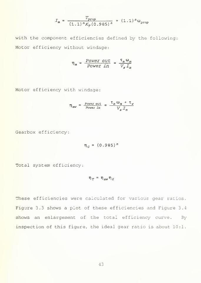
with the component efficiencies defined by the following

Motor efficiency without windage:

Power OUt ^m^ma ' Power in ' Vg lm3 ID

Motor efficiency with windage

_ _ Power out _m ^m wMaw Powez ±n VI

Gearbox efficiency:

r\ G = (0.985) n

Total system efficiency:

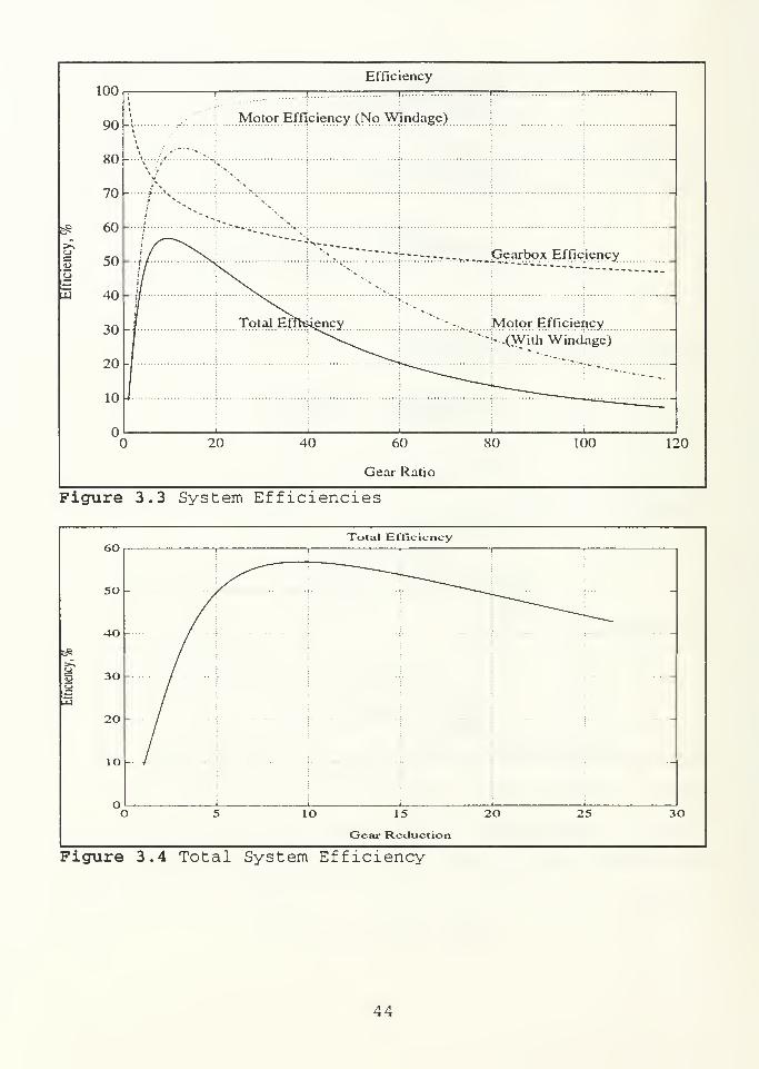
These efficiencies were calculated for various gear ratios.

Figure 3.3 shows a plot of these efficiencies and Figure 3.4

shows an enlargement of the total efficiency curve. By

inspection of this figure, the ideal gear ratio is about 10:1.

43

d^

UJ

100

90

80

70

60

50

40

30

20

10

Efficiency

-

Motor Efficiency (No Windage)

....

.-'

;/ >v "'*! " --"- 5?ear^ox Efficiency

Total Efficiency " - ..^ Motor Efficiency

\. * > .(With Windage)

^^-^^

i i i i

20 40 60

Gear Ratio

80 100 120

Figure 3.3 System Efficiencies

Total Efficiency60 T !

50

AO

30->

UJ

20

io

O() 5 io 15 20 25 3O

Gear Reduction

Figure 3.4 Total System Efficiency

44

3.6 Sensitivity of the Analysis

This analysis was carried out using several different

stage reduction ratios and efficiencies. The effects of

changing these parameters are summarized below.

1. Changing the stage reduction ratio only from 1.1:1 to

4:1 had little effect on the gear ratio where the peak

efficiency occurred. It did effect the height of the peak

significantly.

2. Varying the stage efficiency alone (fixed 1.1:1 stage

reduction ratio) had little effect on the peak location while

the stage efficiency was above 95%. Below 95% the peak moved

to lower gear ratios.

3. Varying both the stage reduction ratio and efficiency

in a coordinated manner to maintain 80% efficiency at a 4:1

gear ratio, had no significant effect on both peak location

and height

.

In general, the model of the gearbox and motor developed

in this chapter is relatively insensitive to the assumptions

made about the gearbox. The windage loss dominates the peak

efficiency curve, provided a gearbox with sufficiently high

efficiency is used.

45

Chapter 4

The Lumped Parameter Model

of The Propulsor

4.1 Introduct ion

ABE will incorporate a complex control system designed to

allow the vehicle to operate independently for periods of up

to twelve months. In order to accomplish this mission, ABE

must have extremely efficient thrusters and an efficient

control algorithm. The control algorithm must be based on a

simple, yet accurate model of the thruster. In this chapter

a lumped parameter model of the thruster is developed and

presented in bond graph notation. A simulation of this model

was performed using MATLAB, and the results are compared to

experimental data in Chapter 5.

4.2 Description of the Thruster Unit

The thruster under consideration, consists of a DC

brushless motor, a controller for the motor, a 10:1 reducing

gearbox, a three blade propeller mounted in a duct. Figure

4.1 shows a schematic diagram of this assembly.

46

Propeller

& Duct

Cntl

Controller

TSupply

MotorTau-

Omega

Windage

Loss

Tau

Omega

Gearbox

Omega

Tau (LOSS) Tau, (LOSS)a

Figure 4.1. Schematic representation of thethruster unit.

4.2.1 The Propeller and Duct Assembly

The propeller and duct assembly as a unit, has the single

most significant impact on the overall efficiency of the

thruster. Therefore, the model of this unit determines the

accuracy and utility of the overall model. Figure 4.2 shows

the schematic representation of the propeller and duct. In

order to describe the hydrodynamic relationships, the

following simplifying assumptions are made [7]:

1. The ambient fluid is inviscid, incompressible and of

constant density.

2. The gravity effects on the fluid are negligible.

47

3. The flow at the inlet and outlet is parallel to the

thruster axis, (irrotational)

.

4. The only energy storage in the fluid is by kinetic

energy.

5. The kinetic energy of the ambient fluid is

negligible

.

6. The ambient pressure is P and it acts equally at

the inlet and the outlet.

Tau.Omega

P: pitch

A. V

Figure 4.2. The propeller and ductassembly, Schematic Representation.

In order to model the hydrodynamics, first, consider the

Kinetic Co-energy, EK*. This is the typical "Physics Book

Kinetic Energy" {lA mv 2

} .

*Z-±i9V)[** (4.1)

Where pV is the mass of the fluid enclosed by the duct.

However, this volume must be corrected to take account of the

48

added mass effect of the surrounding fluid. This correction

involves a concept known as Added Mass or Virtual Mass . Added

mass is a phenomenon that occurs when a body (or a fluid

element) moves through a fluid. An additional inertia effect

is added to account for the effort required to "push" the

fluid out of the way of the moving body. For the case of a

body moving slowly through a static fluid, the added mass is

equal to the volume of the body times the density of the fluid

(ie. the mass of the displaced fluid) [8] and [9] . For this

model (where the density is constant) this is done by setting

V to twice the actual enclosed volume. Q is the volumetric

flow rate. A is the cross-sectional area of the duct. Now,

define the pressure momentum, T, as:

r A -±{e'k )= -£*£ (4.2)

**Note that there is a linear relationship between V and

Q. This is analogous to the standard translational definition

of momentum, p=mv, and leads to the numerical equality of the

Kinetic Energy, E K and the Kinetic Co-energy:

i - frdo - \(4.3)

ir-fQdr-f£$dr- a 2 t2

2pVA 2

2p V A'= pVQ'4

2 A 2- E'K

49

In Summary

EK -E>K - SLISL = ±*H (4.5)K K2A 2 2pV

r =-eZ2 And 0=^ (4.6)A 2 pV

Now consider a power balance for the propeller and duct.

Power in:

The power flow into the duct comes from three major

components: 1) The driving motor, 2) Any Kinetic Energy

flowing into the thruster inlet, and 3) The velocity/

opposing-force product at the inlet ( work done by the fluid

entering)

.

1. The power input from the motor/gearbox is the product

of the torque, X, and the angular velocity, co.

2. Since it is assumed that the ambient fluid is at rest,

there is no kinetic energy flow into the thruster.

3. The velocity/force power is the product of ambient

pressure P and the cross-sectional area and the fluid

velocity at the inlet

.

50

Pin = TU +(Po^)|-f)

+ ^-i, = ™ + PoO (4-7)

Power out

The power flows out of the duct by two processes. The

first is the force/velocity work at the discharge. The second

is the kinetic energy of the discharged fluid. This latter

flow is called the convected kinetic energy.

1. Since the cross-sectional area is constant and the

average velocity of the fluid is the same at the inlet and

outlet, this term is the same as the corresponding term at the

inlet, P Q.

2. The convected kinetic energy is the kinetic energy per

unit volume times the volumetric flow rate:

K = Convected Kinetic Energy = —£ \Q\ =a2 **

l

gi (4.8)

V 2pV2

a z v2 in

l

Pouc - PoO - V I

fI (4-9)

2 p V-

Note: the absolute value preserves the sign of the convected

kinetic energy to allow for flow reversal.

51

Balance of Power:

The net rate of change of the energy in the fluid

contained in the duct is equal to P in -Pout .

d-ET - Pln - Pout = xc + Po- Po

- ^M = TW - ^ icldt r « ouc o- o- 2py2 2py2

Since the only method of energy storage within the duct

is through kinetic energy:

d pi _ d r? _ dr

a 2r2>

|. A*r t _ TCJ

A 2r2|g| (4 .n)

l2pW p V 2 p ^2

This leads to the first state equation

p _ py-co) _ rio|

A 2 Y 2V(4.12)

However, Q=Q(r)=Q(co) therefore we can write V as r(co) and

reduce equation (12) as follows:

1. Define p as the pitch of the propeller. This quantity

is also known as the advance of the propeller. Specifically,

p is the distance the propeller travels axially per revolution

in an "ideal" fluid.

2. Define r\ , the propeller's efficiency, is equal to 1-CF;

where a is the slip of the propeller: [7]

52

a a" pA ~ 2n° (4.13)

upA

Now we can write T and Q in terms of CO.

= ID P T) A {4.14)271

where Q = (rev per sec) * (pitch) * (efficiency) * (Area)

= Volumetric Flow rate

r = Pipy (4.i5)2nA

Using equations (4.6) and (4.15), we can rewrite equation

(4.12) as:

t = 27tT _ ^ 2 r[r| = 2ttt _ pQ\Q\ (4.16)pr\A 2pV2 pr)A 2A 2

This equation can easily be written in terms of CO:

d) = 4 * 2t _P^"M (4.17)p 2

T]2 pV &nV

From these equations we get the bond graph shown in Figure

4.3.

53

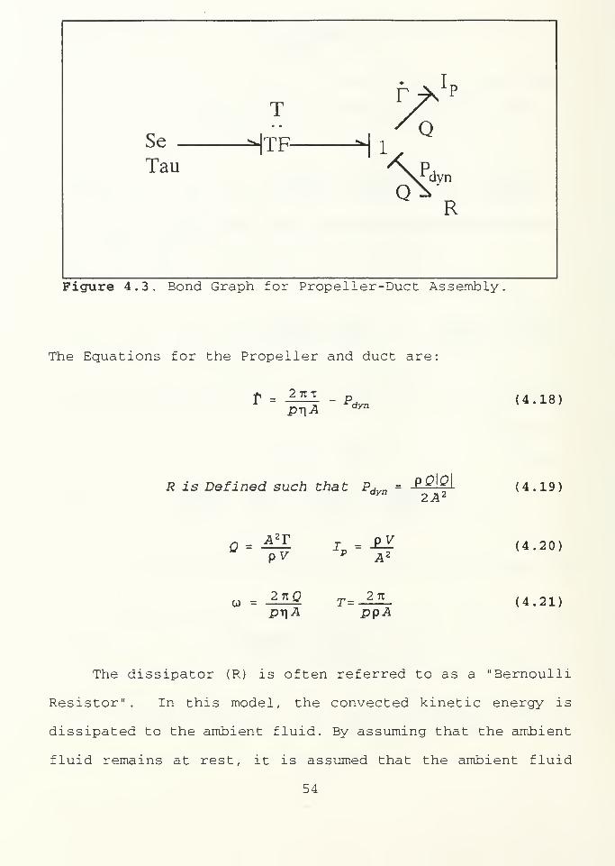
Figure 4.3. Bond Graph for Propeller-Duct Assembly.

The Equations for the Propeller and duct are:

r = AEi - p„,„, (4.18)pi]A dyn

R is Defined such that Pdvn = P°\ Q \ (4.19)dyn 2A ?2

o=^L r = £¥ (4<20)pV p A 2

w = 27tQ T= 2tt (4.21)

The dissipator (R) is often referred to as a "Bernoulli

Resistor". In this model, the convected kinetic energy is

dissipated to the ambient fluid. By assuming that the ambient

fluid remains at rest, it is assumed that the ambient fluid

54

acts as an infinite sink for this energy, much the same as is

considered for the thermal energy dissipated by an electrical

resistor [10 ] .

The parameters for the propeller are: p=0.41 meters/rev.,

Propeller efficiency is 60%, A= 0.164 m 2, corrected volume is

0.033 m3.

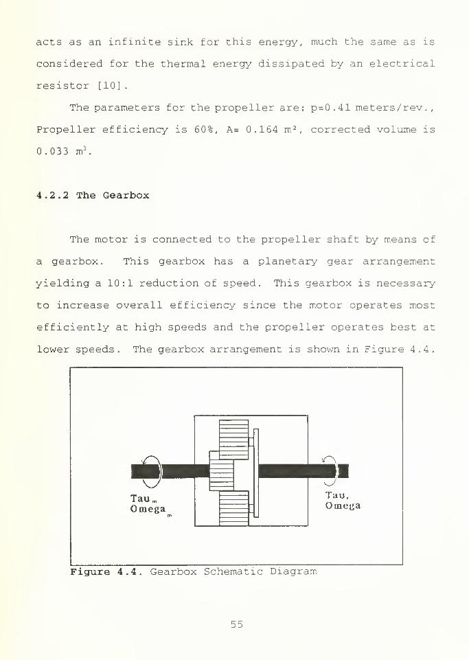
4.2.2 The Gearbox

The motor is connected to the propeller shaft by means of

a gearbox. This gearbox has a planetary gear arrangement

yielding a 10:1 reduction of speed. This gearbox is necessary

to increase overall efficiency since the motor operates most

efficiently at high speeds and the propeller operates best at

lower speeds. The gearbox arrangement is shown in Figure 4.4.

/~> om^M mifflBwmv7

Tau mOmega

m

Tau,Omega

Figure 4.4. Gearbox Schematic Diagram

55

The gearbox used has an 80% efficiency at top speed

(input shaft maximum speed is 10,000 RPM) . This means that

there is a dissipative element as well as a torque

multiplication. The inertial load of the gearbox will be

included with the motor's rotor inertia. Defining xm as the

motor output torque, x x as the gearbox output torque, 0) as the

input shaft speed, and o^ as the output shaft speed, the

gearbox can be modelled as shown in the block diagram of

Figure 4.5 .

Figure 4.5. Bond Graph for Gearbox.

The equations describing the gearbox are

*G =0.2x

0).

NG =10 (4.22)

*=NG^m- xd') td.±2U±.0.2x.

to max

(4.23)

56

JG will be combined with other inertias into an equivalent

inertia

.

4.2.3 The Motor

The motor used is a Pittman elcom © DC Brushless motor.

It is controlled using a +/- 10 VDC control voltage and a

supply voltage ranging from 30 to 80 Volts DC. In this

application the supply voltage is chosen to be 48 VDC. In

order to simplify the model, the supply and control voltages

are "tied" together. This idealizes the controller portion of

the model by assuming no losses in the amplification. The

motor diagram is shown in Figure 4.6 .

48 Vdc Supply1

Control 1 erDC Brushless

Motor

Tau^O mega

1

Control Voltage O to +/- lO \f Ac

Figure 4.6. The Motor Assembly.

57

In order for the motor to operate on the ocean floor, it

must be surrounded by a non-conductive fluid that is

compensated to be at the same pressure as the environment

(10,000 psi) . The fluid in use is a silicon based oil called

Halocarbon © 0.8 cSt. This oil adds a significant windage

loss to the motor ( « 5.2 x 10" 5 Nm/(rad/sec) )

.

The motor is then modelled by Gyrator, a mechanical

inertia and dissipator, and an electrical resistance and

inductance. [11] The gyrator constant is 0.173 Nm/Amp or 0.173

V7 (rad/sec) . The stator resistance RT=4.85 Q, the stator

inductance Lm = 1.65 mH, the combined rotor and gearbox moment

of inertia J r=38.6 x 10" 6 Kg m 2

.

These numbers are from the manufacturer's specifications. The

resulting bond graph is shown in Figure 4.7 .

Figure 4.7. The motor bond graph

58

The resulting equations model the motor:

^ = *i " Jr&>* ~ **<•>» < 4 ' 24 >

x, = KTIm (4.25)

^ck = KE^m (4.26)

T . 1** = T"[ Octroi " ^c/c " ^r-Tlf] < 4 ' 27 >

4.3 The Complete Thruster Model

The complete model is shown in Figure 4

B M.K. \ f\ 7 4:1 2 pi pel. A To

S. —H TF—^ 11—^GY-^0 —iT—^tTF—H 1—H TF—* 1

VC vj Parn^Q

I:LcRw R b

Figure 4.8

59

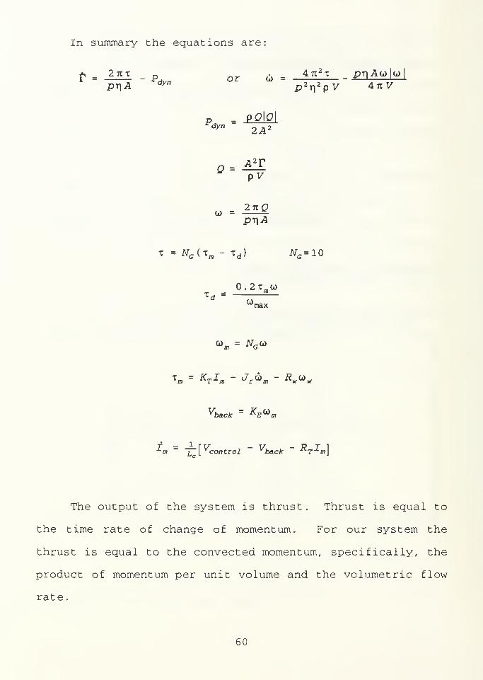
In summary the equations are:

r = un _ Pw r o = 47t2x - P^"l<*pr\A dyn

p 2t]

2 pV 4nV

Pw,= petal

a 2 vo = —

-

*d ="max

C0m = iVG G>

*m = KTIa - Jt dm - RW (D W

Vback ~ KE (jim

The output of the system is thrust. Thrust is equal to

the time rate of change of momentum. For our system the

thrust is equal to the convected momentum, specifically, the

product of momentum per unit volume and the volumetric flow

rate

.

60

Thrust - ( momentum per unit volume ) Q =

Thrust can also be written in terms of CO:

ATV Q = A^TjTj

p V2

Thrust = *P^P"I"47l 2

The bond graph representation of Figure 4.8 can be put

into block diagram form. The resulting block diagram of the

complete thruster unit is shown in Figure 4.9.

Desired ^W# \

Thrust ^S\ T1

'„

Lcs RT

Figure 4.9 The Complete Model Block Diagram

61

This model contains the electrical dynamics of the motor

as well as the hydrodynamics of the propeller. The electric

time constant LC /RT =0.34 milliseconds. This is extremely fast

compared to the hydrodynamic time constant which is on the

order of a second. Therefore the hydrodynamics dominate the

electrical and the later can be neglected without degrading

the model. The resulting model is shown in Figure 4.10 . The

model presented here has been simplified to correspond to the

model used in reference [12].

DesiredThrust

1+ f

a1

s

rPriCt -Thrust

Figure 4.10 The Simplified Model Block Diagram

Where Rw is neglected since Rw < J and

62

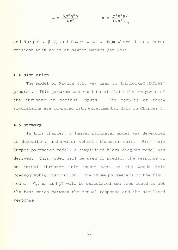
c = ^p 2Ti

2p a m p 2

r)2 pA

T4ti 2 ien'JQQ

and Torque = P Vc and Power = TO) = (3vcco where p is a motor

constant with units of Newton Meters per Volt.

4.4 Simulation

The model of Figure 4.10 was used in MathWorks© MATLAB™

program. This program was used to simulate the response of

the thruster to various inputs. The results of these

simulations are compared with experimental data in Chapter 5.

4 . 5 Summary

In this chapter, a lumped parameter model was developed

to describe a underwater vehicle thruster unit . From this

lumped parameter model, a simplified block diagram model was

derived. This model will be used to predict the response of

an actual thruster unit under test at the Woods Hole

Oceanographic Institution. The three parameters of the final

model ( CT , a, and P) will be calculated and then tuned to get

the best match between the actual response and the simulated

response

.

63

Chapter 5

Experimental Verification

The next consideration is to show that the model

developed in Chapter 4 is competent to describe the actual

thruster. This will be done in three steps. First, by

equating the steady state responses of the model and the

experimental thruster. Second, the model will be tuned to

match the thrusters step response. Finally, the actual and

predicted responses to several frequencies of sinusoid will be

examined. The model's ability to correctly predict the

sinusoidal response will be evaluated.

5 . 1 The Experimental Setup

For the purposes of model verification, an MFM ™ DC

brushless motor (electrically comparable to the Pittman motor

described in Chapter 4) with a 10:1 gearbox, was mounted in a

housing filled with Halocarbon fluid. The experimental

propeller (Michigan Wheel 3-blade 16-inch pitch propeller) was

mounted on the gearbox output shaft and supported radially by

an external journal bearing. A frame was constructed to hold

the motor housing and bearing assembly. The frame is

64

supported at a single pivot point with a lever arm extending

upward to allow force measurement to occur out of the water.

Figure 5.1 shows the arrangement of the frame and the force

measurement sensor. The force sensor is an S-type load cell

rated at 500 pounds-force.

Load Cell

Lever Arm

rmPtvot

Instrument

Cabres

I Beam

Figure 5.1 The Experimental Test Stand

After initial testing, the test frame was reinforced to

reduce the oscillatory effect of the vertical lever arm

compliance. This reinforcement significantly reduced the

"ringing" of the thrust measurement. In order to remove

gravity effects, the test assembly was balanced before each

data run, so the vertical lever arm was straight up and down.

The force sensor was arranged to measure the horizontal

component of force at the end of the vertical arm. This

arrangement decouples all gravitational effects of the motor

and propeller from the force measurement.

65

5.2 Steady State Response

The constants of the model developed in Chapter 4, (CT ,

a, and (3) were adjusted so the model accurately predicts the

correct steady state response of the thruster for thrust,

angular velocity, and power input required. This process

determined CT and P directly.

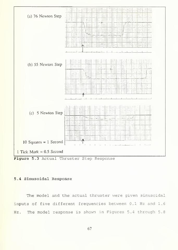
5 . 3 Step Response

The step response data collected with the experimental

thruster was used to determine the a parameter. The modelled

response to three separate step inputs is shown in Figure 5.2

and the actual response is shown in Figure 5.3 (a,b,&c)

.

Desired and Actual Thrust

70,.-'"

-

601

-

c2*

Z.

50

40

i ;

JO

20

;

// ,.-

..-—"

10 //

(

*/

) 0.5 1 1.5 2 2 5

Time, Seconds

Figure 5.2 Model Step Response

66

(a) 76 Newton Step

[|t: ifii iiti

-i—i—i—

i

f

M

U4-4li^0l

v*-vf

:.:.

;::

...:

::::

mm-I I 1 1 1 1 1 1 1 1 1 1 u

(b) 55 Newton Step

M

ii

iiEv^L

....

IjTi

¥

in

... ~

....

....

.... ...

I I l I I l_—

J

1 1 1 1 1 1 1 1 1 1 I

(c) 5 Newton Step

10 Squares = 1 Second

1 Tick Mark = 0.5 Second

H MilMil 1 | III!

i

1

1

Ijii

rli! f;i] :

n 1 i ! ! p RTTH>- mt miin

Ij-tii:i

;

IM

1 rrrJ

T"t it T" "t "t itf

;j| 1J

:

':! 1

:

II i I-IM III

j

1 1

j

III

iX+ i U illHi!1:11

il 1 :i

A ' U mi ii li :

!

|

:

ii

1 1 1 1 1 1 - - - 1 .1 . 1

—

1

Figure 5.3 Actual Thruster Step Response

5.4 Sinusoidal Response

The model and the actual thruster were given sinusoidal

inputs of five different frequencies between 0.1 Hz and 1.6

Hz. The model response is shown in Figures 5.4 through 5.8

67

sub-plot (a) . The actual response is shown in subplot (c) of

the same figures. Note that the actual response is inverted.

The time scale is .1 second per finest square. The force scale

is 5.7 N per smallest division.

Time Scale: 10 Squares = 1.0 Seconds or 1 Tick Mark = 0.5 Seconds

Figure 5.4 Sinusoidal Input T=10 seconds, (a) Model Input andResponse, (b) Actual Input, (c) Actual Response

68

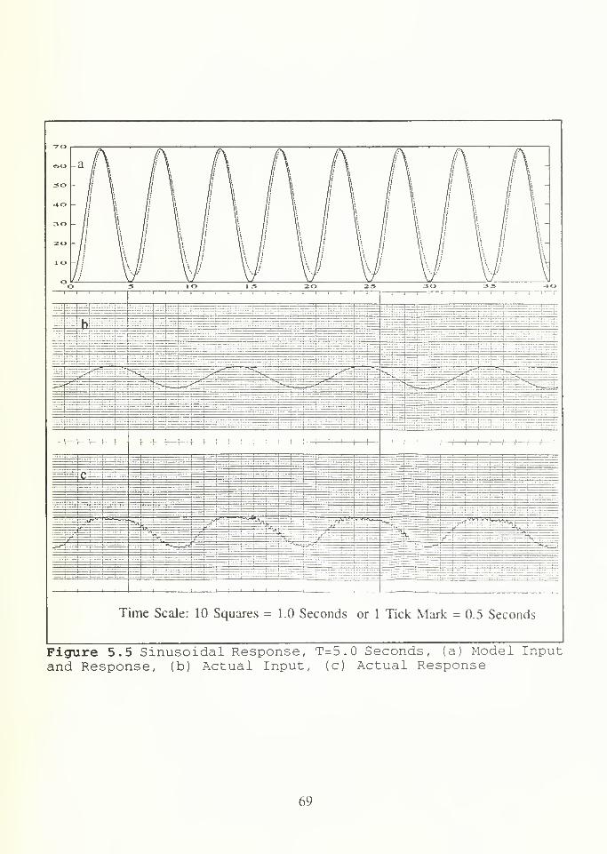
Time Scale: 10 Squares = 1.0 Seconds or 1 Tick Mark = 0.5 Seconds

Figure 5.5 Sinusoidal Response, T=5.0 Seconds, (a) Model Inputand Response, (b) Actual Input, (c) Actual Response

69

1111 H—1-H-+ H 1 r

Time Scale: 10 Squares = 1.0 Seconds or 1 Tick Mark = 0.5 Seconds

Figure 5.6 Sinusoidal Response, T= 2.5 Seconds, (a) ModelInput and Response, (b) Actual Input, (c) Actual Response

70

I I I I I i^^r_! 1 1 I 1 l_I I ! I II—I-

Time Scale: 10 Squares = 1.0 Seconds or 1 Tick Mark = 0.5 Seconds

Figure 5.7 Sinusoidal Response, T= 1.25, (a) Model Input andResponse, (b) Actual Input, (c) Actual Response

71

-I 1 1 r -i 1 1 1 1 11- H 1—f—

I

f- H—I—

h

i i 1^*—r—)

—

h

Time Scale: 10 Squares =1.0 Seconds or 1 Tick Mark = 0.5 Seconds

Figure 5.8 Sinusoidal Response T=0.625, (a) Model Input andResponse, (b) Actual Input, (c) Actual Response.

72

By inspection of the sinusoidal responses, it is seen

that the model accurately predicts the magnitude and the time

lag of the actual thruster. This lag is firmly rooted in the

hydrodynamics of the propeller. The time scale of this lag is

the time necessary to develop the helical wake field down

stream of the propeller after changes occur that effect the

propeller's angular velocity. The model predicts the

magnitude of this lag within 0.1 seconds of the actual

response. The magnitude prediction is degraded for

frequencies over 1 Hz where it under predicts the actual

thrust developed by up to 40%.

5 . 4 Summary

The model developed in Chapter 4, and tuned in this

chapter to match steady state and step responses, does a good

job at predicting the dynamic response of the thruster.

During the experimental studies, the actual thruster response

is highly dependent on the adjustment of the controller to

account for the inertia of the propeller. The controller used

has two modes of operation: Torque control and Velocity

control. The velocity control mode was very sensitive to the

propeller inertia. If the controller is not well tuned, the

velocity control mode becomes unstable. This risks damage to

the mechanical linkages and uses a large amount of electrical

power. Since this undesirable trait was not readily

73

correctable, all the comparisons use the controller's torque

control mode. The model was tuned to best fit the controller

when the controller was matched to the experimental propeller.

In the next chapter, the model and controller were tuned to

other motor and propeller combinations. The method of this

chapter was used to tune all configurations tested.

74

Chapter 6

Steady State Performance Comparison

of Several Thruster Units

6.1 Introduct ion

The purpose of this thesis is to design the best thruster

unit for ABE. In order to verify the performance, the

experimental thruster unit will be compared to other

combinations of propellers and motor/gearbox units. In this

chapter, four separate propellers and two motor/gearbox units

are tested to determine steady state Power required to obtain

a certain thrust at a bollard pull. The test setup described

in Chapter 5 was used to gather the data. The results of

these tests are compared to determine which thruster has the

lowest power consumption over the desired range of thrust.

The motors/gearbox units under test were:

1. MFM Technology Inc. Series SM64 DC Brushless

Motor with a 10:1 Gearbox.

2. Pittman elcom Series 5100 DC Brushless

Motor with a 4:1 Gearbox.

75

The Propellers used in these tests were:

1. JASON Thruster Propeller; a 2-blade, 10-

inch diameter propeller with a 4-inch pitch.

2. 18-inch diameter, 2-blade, model airplane

propeller with a 6-inch pitch.

3. 18-inch diameter, 2-blade, model airplane

propeller with an 8-inch pitch.

4. 18-inch diameter, 3-blade, Michigan Wheel

Sailer Marine propeller with a 16-inch pitch.

(This is the EXPERIMENTAL Propeller)

Each combination of these components was tested in the

two controller modes, Torque and Velocity control.

The "experimental" thruster consists of the MFM motor

with the 10:1 gearbox and the Michigan Wheel propeller.

6.2 The ABE Thruster and Other Thruster Units

The thruster units will be categorized by the propeller

used. The discussion starts with the smallest propeller and

ends with the experimental propeller.

76

6.2.1 The JASON Propeller

The first propeller considered is the propeller from a

JASON vehicle thruster. This propeller is used by the

tethered underwater vehicle JASON and is equivalent to a

standard 2-blade Mercury outboard motor propeller. Figure 6.1

shows the response of the JASON propeller to each

motor/gearbox unit and controller mode. In this chapter the

graph labels are decoded as follows:

The first letter indicates the motor unit under

test, M corresponds to the MFM motor (10:1

reduction) and P corresponds to the Pittman Motor

(4:1 reduction)

.

The middle 2 or 3 letters/numbers indicate the

propeller used. JAS = the Jason Propeller, 86 = the

18" diameter 6" pitch airplane propeller, 88 = the

8" pitch airplane propeller, 316 = the Michigan

Wheel 3-blade 16" pitch propeller.

The last letter indicates the controller mode, T =

torque control, R = velocity control.

Examination of Figure 6.1 shows for the range of -10 to

+10 Ibf thrust, the Pittman motor/ 4:1 gearbox in torque mode

outperforms the other methods of powering the JASON propeller.

77

For the 100 Watt ABE power budget limit, this unit provides a

range of thrust from -8 lbf to +9 lbf at bollard.

Propeller JASON

300

250

a3 200

I 150

3Q.

3100

50

-:

PlASR I/

MJASR i, /.:

PJAST\,). \ A--''

A

5 -20 -15 -10 -5 5 10 15 20 2

ThmsUbf

5

Figure 6.1 The Jason Propeller Response

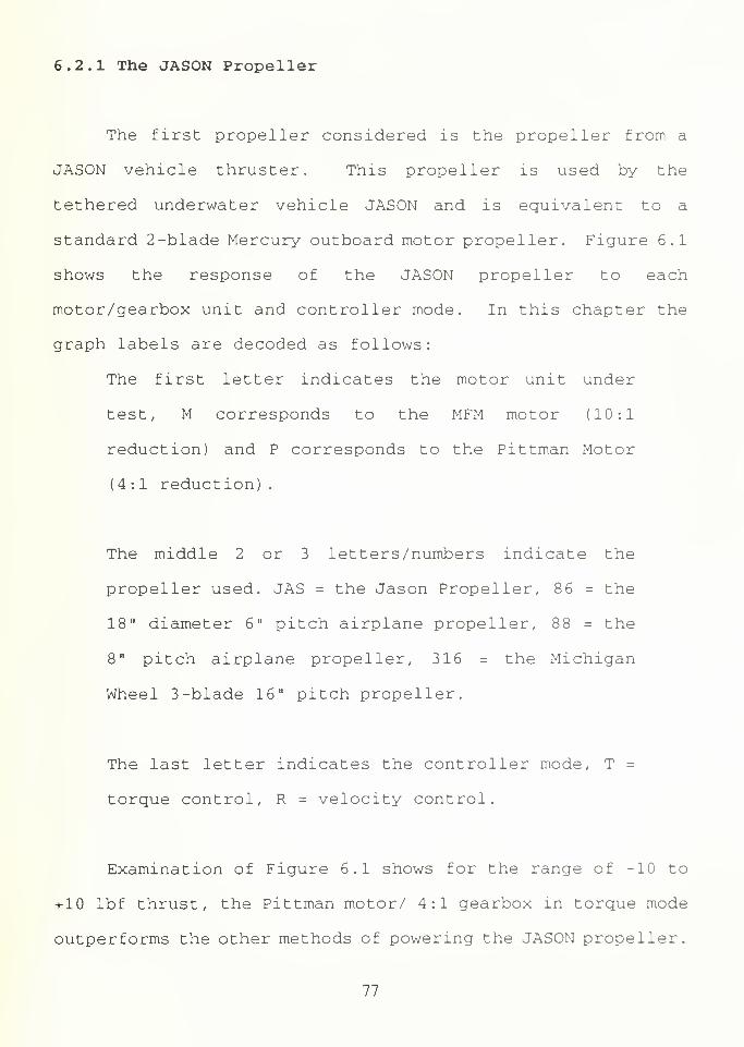
6.2.2 The 86 Airplane Propeller

The second propeller is the 18-inch diameter model

airplane propeller with a 6-inch pitch. This propeller is

extremely asymmetric and is designed to be operated in only

one direction. Figure 6.2 shows the steady state data for

this propeller. Note the large difference in power required

between forward and reverse thrust. For the +/- 10 lbf thrust

range all thruster unit combinations are comparable, with the

MFM motor in torque mode being the best. For ABE's 100 Watt

limit, this propeller can provide -5 lbf to 12 lbf

78

Propeller S6

soo

250 -

g 200M86R P86R

l , ;/ -

*

J-

150

\ P86T vjy

'M A^XLOO

\ //so

A j^y\ j'"^'\?

0,.

.5 -20 -15 -10 -5 5 10 15 20 25

Thrustjbf

Figure 6.2 The 86 Airplane PropellerResponse

6.2.3 The 88 Airplane Propeller

The 18-inch diameter model airplane propeller with an 8-

inch pitch is very similar to the 86 propeller above. Figure

6.3 shows the data collected for this propeller. Again the

MFM motor in torque mode outperforms the other combinations.

The range of thrust available within the 100 Watt limit is -7

lbf to 13 lbf. This is slightly better than the 86 propeller

performance

.

79

Propeller I

300-

250

200-

150 -

100 -

50-

M88T

,, I I $?ii

, V vast///),

\Jj\ msmt'V., I

-!

' \V V^-- i i i -

-25 -20 -15 -10 -5 5 10 15 20 25

Thrustjbf

Figure 6.3 TheResponse

18 Airplane Propeller

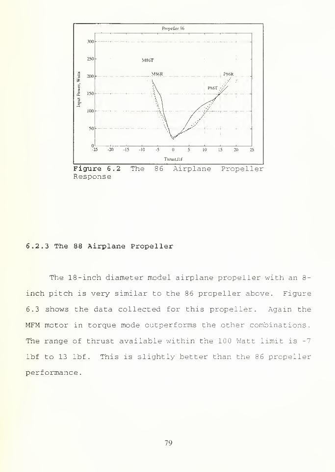
6.2.4 The Experimental Propeller

The last propeller considered is the experimental

propeller described in Chapter 2. This propeller, when

matched with the designed motor/gearbox unit, outperforms the

4:1 gearbox in both controller modes. The range of thrust

available under the 100 Watt limit is -7.5 lbf to 11 lbf.

This propeller has the best bi-directional response of any of

the tested propellers. Figure 6.4 shows the data for this

propeller

.

6.3 Steady State Comparison

Due to the limitation of the controller mentioned at the

end of Chapter 5, the velocity control mode was not used for

80

Propeller 316

300

250

?16R

T 1 !

V P316T

P316R/:'•',

3 200M31OT V, ,'!

\ ^

,','

ioa. 150

\ \

1 '

3

tI /

ion

50

5 -20 -15 -10 -5 5 10 15 20 25

Thrustjbf

Figure 6.4 The Experimental PropellerResponse

the final comparisons of the thruster units. The velocity

mode shows a marked instability that is highly dependent on

the inertia of the attached propeller. This instability

causes an excess of power to be drawn at various speeds of

operation, including stopped. Since the controller cannot be

readily tuned to each propeller, the comparison of thruster

units will be made with the data from the torque mode tests.

Ideally, the steady state power consumption of the velocity

mode can be tuned to a value close to the power used in the

torque mode. The deficiency in this controller will be

commented on in Chapter 8.

In general, the MFM motor with the 10:1 gearbox surpasses

the Pittman motor with the 4:1 gear reduction. The only

exception is the JASON propeller, which performed best with

the Pittman motor unit. Since the motors are electrically

SI

comparable, it can be inferred that the 10:1 gearbox is a

better choice for the 88, 86 and 316 propellers.

The JASON propeller has the most limited range of thrust,

regardless of power input. The maximum thrust for this

propeller is near +/- 10 lbf. This gives insufficient thrust

for ABE's sprint capability of 2 knots (requiring about 13

lbf) . Due to this limitation, the JASON Propeller will not be

considered further.

Figure 6.5 shows the comparison of the propellers using

the MFM motor in torque control and the 10:1 gearbox. For the

forward thrust direction below 13 lbf, the 88, 86, and 316

propellers have nearly the same thrust/power characteristic.

Since this Is the region of interest, there is little to

differentiate between the propellers. However, ABE will be

operating in an area of current gradients. This means that

forward and reverse thrusts will be necessary to maintain

constant velocity while traveling on a closed circuit

trajectory. Reverse thrust will also be necessary while ABE

is maneuvering at docking. Therefore, the main propulsion

thrusters should have the best possible reverse thrust

efficiency without severely effecting the forward thrust

characteristic. The 316 propeller has the lowest power

consumption for any astern thrust demand. For comparison

purposes, Figure 6.6 shows the velocity mode control curves

for the MFM motor and all propellers. The tuning of the

82

controller increases the separation of the 316 curve from the

other curves

.

300-

250

(i

Torque Mode Propeller Curves

-i r-

M88T

MXbT

-25 -20 -15 -10 -5 5 10 15 20 25

Thrust, lbf

Figure 6.5 Propeller Comparison, TorqueMode, MFM Motor

Velocity Mode Propeller Curves

300\ M316R

250

a 200M88R

$ v M«6R

ia— 150 \ //'

3

£ \ ' •'''?

100\ ';• MJASR ,-' /

y

•

so

5 -20 -15 -10 -5 5 10 15 :o :5

Thrust, lbf

Figure 6.6 Propeller Comparison, VelocityMode, MFM Motor

83

6 . 4 Summary

For steady state operation, the experimental thruster

consumes less power than any other unit considered. In the

range of - 10 lbf to + 10 lbf thrust demand, the experimental

thruster has a power consumption advantage of 12% over the

nearest competitor. This assumes that the thruster operates

over a given trajectory, where any changes in thrust occur

slowly and there is an equal demand of forward and astern

thrusts. Chapter 7 examines the case where these assumptions

are not valid.

84

Chapter 7

Balancing Dynamics and Efficiency

7 . 1 Introduction

Chapter 6 compared the combinations of propellers and

motor/gearbox units in steady state. Although this gives

important insight into the performance of the thrusters, this

is only a small portion of the story. ABE will rarely operate

in a "steady state" environment. During ABE ' s flight along a

preprogrammed trajectory, there will be accelerations,

constant velocity runs and unknown current gradients. These

factors will drive ABE away from the steady state toward a

richly dynamic environment

.

In this chapter, the experimental propeller will be

compared with the two model airplane propellers presented in

Chapter 6. The experimental propeller will be driven by the

MFM motor with the 10:1 gearbox. The airplane propellers will

be combined with each of the two motor/gearbox units. The

comparison will be based on the model of Chapter 4, with the

parameters experimentally determined for each thruster. These

parameters are shown in Table 7.1 . The following definitions

apply to Table 7.1:

85

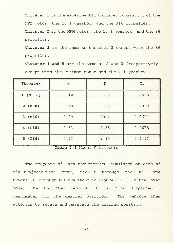
Thruster 1 is the experimental thruster consisting of the

MFM motor, the 10:1 gearbox, and the 316 propeller.

Thruster 2 is the MFM motor, the 10:1 gearbox, and the 88

propeller.

Thruster 3 is the same as thruster 2 except with the 86

propeller

.

Thruster 4 and 5 are the same as 2 and 3 (respectively)

except with the Pittman motor and the 4:1 gearbox.

Thruster a P CT

1 (M316) 0.10 23 .0 0.0660

2 (M88) 0.18 27.0 0.0820

3 (M86) 0.09 20.0 0.0677

4 (P88) 0.33 2.85 0.4678

5 (P86) 0.23 2.85 0.4497

Table 7 . 1 Model Parameters

The response of each thruster was simulated on each of

six trajectories: Hover, Track #1 through Track #5. The

tracks (#1 through #5) are shown in Figure 7.1 . In the Hover

mode, the simulated vehicle is initially displaced 1

centimeter off the desired position. The vehicle then

attempts to regain and maintain the desired position.

86

0.6

0.4

0.2

(

0.6

0.4

| 0.2

-0.2

(

Simulation Velocity Tracks

/' Track2&3

Track 1

) 5 10 15 20 25

Time, Seconds

Track 4

30 35 40

-

Track 5

\ \

) 5 10 15 20 25

Time, Seconds

30 35 40

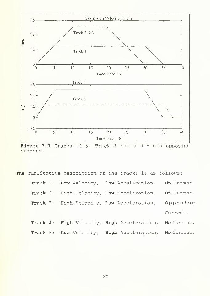
Figure 7.1 Tracks #1-5, Track 3 has a 0.5 m/s opposingcurrent

.

The qualitative description of the tracks is as follows:

Track 1: Low Velocity, Low Acceleration, No Current

Track 2: High Velocity, Low Acceleration,

Track 3: High Velocity, Low Acceleration,

No Current

.

Oppo s i ng

Current

.

Track 4: High Velocity, High Acceleration, No Current

.

Track 5: Low Velocity, High Acceleration, No Current

.

S7

7.2 Dynamic Comparison

From step response data for each thruster unit under

consideration, the speed of response can be rated. The

criteria is the time until the thrust output stays within 5%

of the final value. The thrusters were judged for a thrust

step of 50 Newtons (approximately 11 lbf ) . The results are

shown in Table 7.2

Thruster Response Time

M88 . 55 sec

P88 0.60 sec

M8 6 0.60 sec

P86 0.65 sec

M316* 0.85 sec

Table 7.2 Time Response * Experimental Thruster

The 18-inch airplane propeller with an 8-inch pitch has

the fastest response of all the propellers. For small thrust

steps the differences between the speeds of response is large.

For larger steps the time responses approach the same limit.

The experimental propeller has the slowest response of the

tested thrusters.

88

7.3 An Open Loop Force Controller

In order to evaluate the thrusters a simple force

controller will be implemented. This will be a PD controller

with poles placed such that the system's natural frequency is

(On = 1 . rad/sec, and the damping ratio is r\ = 0.707 .

7.3.1 The Simulated Vehicle

In order to test the thrusters on the aforementioned

tracks, some vehicle dynamics must be considered. The vehicle

modelled will be ABE. The drag of the vehicle is the drag

calculated in Chapter 2 . The drag at 1 knot is used to

calculate an effective drag coefficient C' D such that:

C'D = ±pACD = 190^2 (7.1)2 m

The effective mass of the vehicle will be the

displacement of the three main body sections of ABE plus an

added mass term. The added mass is used to account for the

volume of water in and around the vehicle that must be

accelerated in order for ABE to move through the water. For

this analysis, the added mass is assumed to come from a sphere

of water in front of each body section. Each sphere has a

diameter equal to the maximum diameter of the associated

section. The displacement of ABE is approximately 800 kg and

89

the added mass is about 160 kg. This leads to an effective

mass of 960 kg.

Since three thrusters are used to drive the vehicle, and

the point on their operating curves is significant to the

analysis, it is assumed that the three thrusters share the

load equally at all times. This allows the simulation to be

run for one thruster using one third of the values calculated

above. Therefore each thruster will 'see' an effective drag

coefficient of C' D = 22.67 kg/m and an effective mass of 320

kg.

7.3.2 Power Consumption Comparison

Each thruster was run on each simulated track. The

average power during the run was computed and tabulated in

Table 7.3. Initially, it is assumed that the thruster has the

same forward and reverse power to thrust characteristic.

Double line blocks indicate the lowest mean power consumption

for a particular trajectory.

90

Thruster Hover Track

#1

Track

#2

Track

#3

Track

#4

Track

#5

1 (M316) 19.96 24.56 29.30 39.86 34.59 27.65

2 (M88) 19.47 24.53 29.96 41.56 35.61 27.24

3 (M86) 20.19 24.72 29.42 39.99 34.73 28.45

4 (P88) 19.85 26.26 33 .17 47.98 40.50 30.16

5 (P86) 20.26 25.00 29.92 40.99 35.49 28.96

Table 7.3 Mean Power Consumption in Watts

The assumption of equal ahead and astern performance is

not valid (see Chapter 6, Figure 6.5) . A penalty factor must

be applied to each thruster to correct for the increased power

consumption in the astern thrust direction. The penalty

factor (PF) used in this analysis is the ratio of slopes from

the steady state power versus thrust characteristic for each

thruster (Figure 6.5) . The penalty factor for each thruster is

shown in Table 7.4 . In order to apply this correction, some

assumption must be made about the ratio of time at ahead

thrust versus the time at astern thrust. When it is assumed

that the thruster operates between 1/4 and 1/2 of the time

astern, the results for Tracks #1,2, 4, and 5 are the same in

terms of thruster ranking. (ie. the sensitivity to this

91

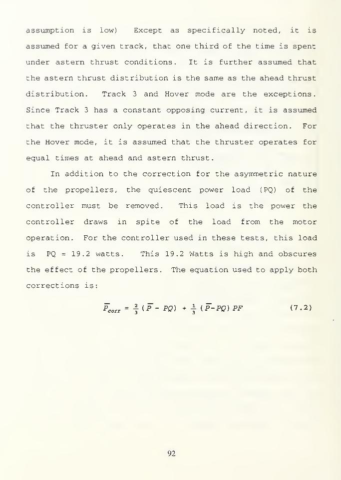
assumption is low) Except as specifically noted, it is

assumed for a given track, that one third of the time is spent

under astern thrust conditions. It is further assumed that

the astern thrust distribution is the same as the ahead thrust

distribution. Track 3 and Hover mode are the exceptions.

Since Track 3 has a constant opposing current, it is assumed

that the thruster only operates in the ahead direction. For

the Hover mode, it is assumed that the thruster operates for

equal times at ahead and astern thrust.

In addition to the correction for the asymmetric nature

of the propellers, the quiescent power load (PQ) of the

controller must be removed. This load is the power the

controller draws in spite of the load from the motor

operation. For the controller used in these tests, this load

is PQ = 19.2 watts. This 19.2 Watts is high and obscures

the effect of the propellers. The equation used to apply both

corrections is:

Peon = | (-P- p0) + -j (P-PQ) PF (7.2)

92

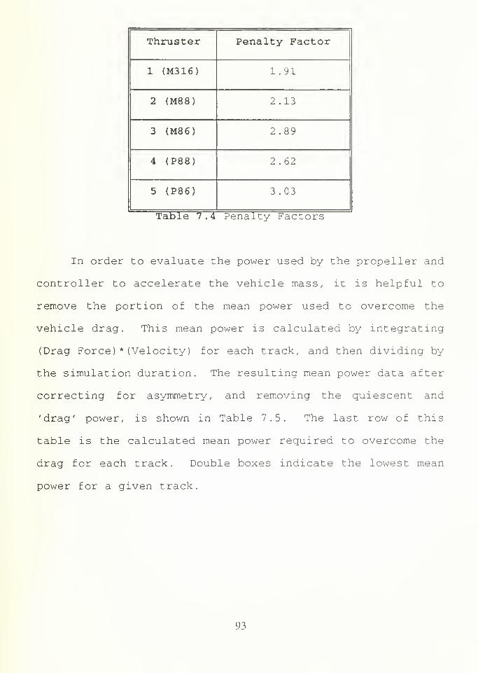
Thruster Penalty Factor

1 (M316) 1.91

2 (M88) 2.13

3 (M86) 2.89

4 (P88) 2.62

5 (P86) 3.03

Table 7.4 Penalty Factors

In order to evaluate the power used by the propeller and

controller to accelerate the vehicle mass, it is helpful to

remove the portion of the mean power used to overcome the

vehicle drag. This mean power is calculated by integrating

(Drag Force) * (Velocity) for each track, and then dividing by

the simulation duration. The resulting mean power data after

correcting for asymmetry, and removing the quiescent and

'drag' power, is shown in Table 7.5. The last row of this

table is the calculated mean power required to overcome the

drag for each track. Double boxes indicate the lowest mean

power for a given track.

93

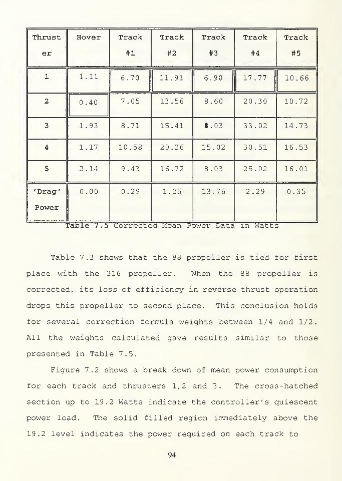
Thrust

er

Hover Track

#1

Track

#2

Track

#3

Track

#4

Track

#5

1 1.11 6.70 11.91 6.90 17.77 10.66

2 0.40 7.05 13.56 8.60 20.30 10.72

3 1.93 8.71 15.41 7.03 33 .02 14.73

4 1.17 10.58 20.26 15.02 30.51 16.53

5 2.14 9.43 16.72 8.03 25.02 16.01

'Drag'

Power

0.00 0.29 1.25 13.76 2.29 0.35

Table 7.5 Corrected Mean Power Data in Watts

Table 7.3 shows that the 88 propeller is tied for first

place with the 316 propeller. When the 88 propeller is

corrected, its loss of efficiency in reverse thrust operation

drops this propeller to second place. This conclusion holds

for several correction formula weights between 1/4 and 1/2.

All the weights calculated gave results similar to those

presented in Table 7.5.

Figure 7.2 shows a break down of mean power consumption

for each track and thrusters 1,2 and 3. The cross-hatched

section up to 19.2 Watts indicate the controller's quiescent

power load. The solid filled region immediately above the

19.2 level indicates the power required on each track to

94

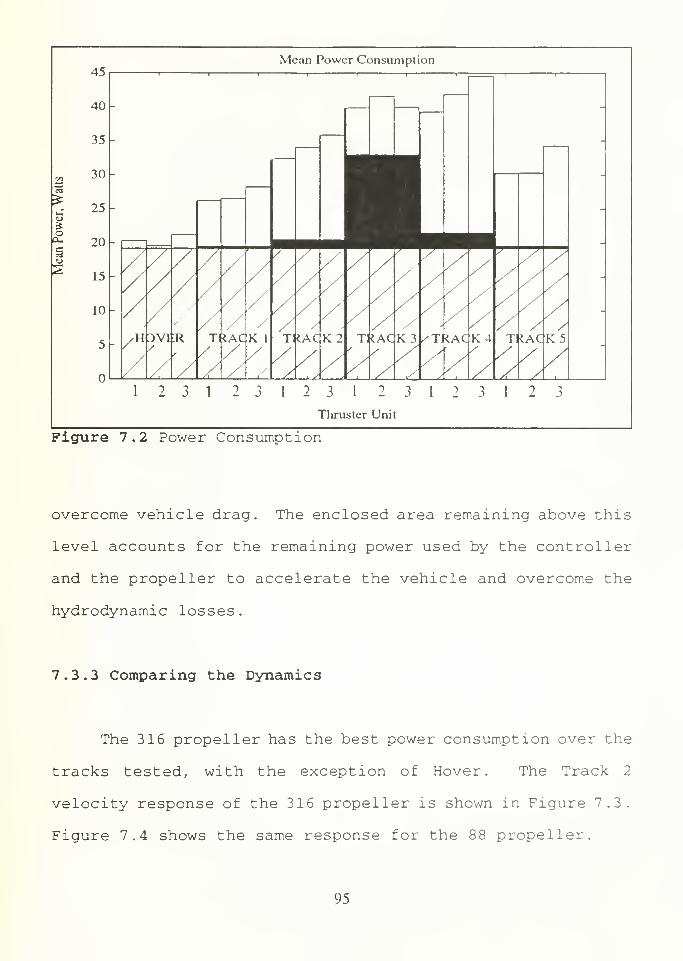
o

45

40

35

30

25

20

15

10

5

Mean Power Consumption

Figure 7.2 Power Consumption

overcome vehicle drag. The enclosed area remaining above this

level accounts for the remaining power used by the controller

and the propeller to accelerate the vehicle and overcome the

hydrodynamic losses.

7.3.3 Comparing the Dynamics

The 316 propeller has the best power consumption over the

tracks tested, with the exception of Hover. The Track 2

velocity response of the 316 propeller is shown in Figure 7.3.

Figure 7.4 shows the same response for the 88 propeller.

95

The position response for both propellers in Hover mode is

shown in Figure 7.5 .

M316 PropeUer, Track #2

0.5 \\

0.4 \

i 0.3 \>>

1>

0.2

0.1

n

-0.1

( ) 5 10 15 20 25 30 35 40

Time, Seconds

Figure 7.3 Experimental Thruster Track#2, Velocity Response

M88 Propeller, Track #2

0.6

0.5 -\

0.4

i 0.3 .

><

1>

0.2

0.1

""

-0.1() 5 10 15 20 25 30 35 4

Time, Seconds

Figure 7.4 The M88 Thruster, Track #2,Velocity Response

96

Hover Position Response

0.01516

0.005

'A

§sE

i ;'/\

\/ \ 1 / i

' \'

1

*

1 /

|\ 1;

l

aoa 1

\ *

'I ' / * 1 •'

1'. 1

•'1

o

-0.005i / / 88 \l' J

\ 1/ / \ I' / \y I vl /

-0.01

-0.015() 5 10 15 20 25 30 35 4

Time, Seconds

Figure 7.5 Thruster Hover Response

7 . 4 Summary

The simulations presented in this chapter show there is

a trade-off between power conservation and rapid dynamic

response. This is clearly illustrated by the data for the

Track 2 simulations presented in Table 7.5, Figures 7.3 and

7.4. The M88 thruster follows the velocity track better than

the M316 thruster. The cost of this slightly improved

response is 2 Watts, a 14% increase over the mean power

consumed by the M316 thruster. This 2 watts, when multiplied

by three forward propulsion thrusters, is 6% of the total

propulsion budget for ABE.

Better dynamics is a more important criteria when

evaluating the hover mode thrusters. By responding quickly,

97

the M88 thruster reduces the magnitude of the hover limit

cycle. This in turn limits the vehicle velocity and power is

saved. This is shown by the plot in Figure 7.5, where the M88

thruster uses 40% of the power used by the M316 thruster.

For a typical ABE track having long constant velocity

legs, rapid dynamics are less important. For a well developed

controller, providing slow acceleration up to survey speed,

the M316 thruster is the optimum choice. The cost in dynamic

response is negligible in this case and the power savings is

significant (14% for Tracks 2 and 4)

.

98

Chapter 8

Summary, Conclusions, and Recommendations

The purpose of this thesis was to develop an optimized

propulsion system for ABE. From the beginning, special

attention was given to maximizing the power efficiency of the

system's components. In this light, a propeller was designed

specifically for the ABE vehicle and its predicted mission

profile. This custom propeller was then matched to a suitable

DC brushless motor. These units were connected via a speed

reducing gearbox, thus taking advantage of the high efficiency

operating regions of both components.

Following its design, the ABE thruster was modelled using

non-linear lumped parameter modelling techniques. The final

model was reduced to three parameters (C T , a, (3) describing

the thruster. Using this model, five different thrusters were

evaluated, including the designed ABE thruster. The three

parameters for each thruster were determined experimentally,

using system identification methods. From the experimental

data and the modelled response, the static and dynamic

performance of the thrusters was compared. Finally, a simple

controller was implemented, and a simulated ABE vehicle with

99

model thrusters, was run on several tracks. This allowed

evaluation of the control performance of each thruster.

The result of this analysis indicates there is a trade-

off between control performance and efficiency. In general,

the designed propeller had the highest efficiency and the

slowest response. The propeller with the fastest response,

demanded more power in order to achieve this improved

performance. The exception is in hover mode where the

improved response limited the vehicle limit cycle and resulted

in power savings. The simulated trajectories were typical of

the predicted ABE track profiles. From these simulations, it

became evident that the power used to overcome hydrodynamic

drag is nearly insignificant for the proposed ABE operating

velocities. The overwhelming share of the power goes first,

to powering the control electronics, then to the un-modelled

hydrodynamics and the power required to accelerate the

vehicle's mass. Therefore, the use of the typical drag

calculation is not sufficient to predict the propulsive power

requirements for ABE.

As the track length increases from the simulated track

length, which is on the order of 10 meters, the importance of

improved propeller dynamics is overshadowed by the need for

higher efficiency. For ABE, this means that the designed high

efficiency propeller is the best choice. The power cost for

the improved propeller response is too high (6-14% as

modelled) and the improvement in velocity tracking is small.

100

Additionally, the limitations imposed by the slower response

of the designed thruster can be compensated for by the

intelligent application of control algorithms. Further

research should start by determining the best way to control

the thruster in order to best exploit its improved efficiency

and to correct for the slow response. Following closely

behind additional control research, should be the coordinated

planning of the ABE trajectories. These tracks must be

developed in a manner that allows the control system to

operate the thrusters at peak efficiency. This includes using

low accelerations and maximizing constant velocity legs as

much as possible. Simulation runs with rapid acceleration to

speed, consumed up to 60% more power than low accelerations to

the same velocity.

101

References

[1] Yoerger, D.R. et al .

; "The Autonomous Benthic Explorer

(ABE) : A Deep Ocean AUV for Scientific Seafloor Survey.";

WHOI #7569; Woods Hole Oceanographic Institution; Sept.

1990.

[2] Kerwin, J.E.; Hydrofoils and Propellers, 13.04 Lecture

Notes ; MIT; January 1991.

[3] Newman, J.N.; Marine Hydrodynamics ; MIT Press; Cambridge,

Massachusetts; 1977.

[4] Abbott, I.H., Von Doenhoff, A.E.; Theory of Wing

Sections ; Dover Publications, Inc.; New York; 1949.

[5] Pittman elcom® Brushless D-C Servomotors , Bulletin 5000,

Technical Data Sheet, March 1989.

[6] Bradley, A.; Woods Hole Oceanographic Institution

Internal Memo; Motor & Gearbox Studies; Fall 19 90.

102

[7] Cooke, J.G.; "Incorporating Thruster Dynamics in the

Control of an Underwater Vehicle"; Engineers Degree

Thesis, MIT/WHOI Joint Program in Oceanographic

Engineering; Woods Hole, Massachusetts; Sept. 1989.

[8] Abkowitz, M.A.; Stability and Motion Control of Ocean

Vehicles ; The MIT Press; Cambridge, Massachusetts; 1969.

[9] Currie, I.G.; Fundamental Mechanics of Fluids ; McGraw-

Hill, Inc; New York; 1974.

[10] Beaman, J.J., Breedveld, P.C.; "Physical Modeling with

Eulerian Frames and Bond Graphs"; Transactions of the

ASME; Vol. 110; June 1988; Pages 182-188.

[11] Ogata, K.; Modern Control Engineering ; Prentice-Hall,

Inc.; New Jersey; 1970.

[12] Yoerger, D.R. et al . ; "The Influence of Thruster Dynamics

on Underwater Vehicle Behavior and Their Incorporation

Into Control System Design"; IEEE Journal of Oceanic

Engineering ; Vol. 15; No. 3; July 19 90.

103

Woodford .

Propulsion optxmiza

tion for ABE, an Autono-

mous Underwater Vehxcle

(AUV)

.

WoodfordPropulsion optimiza-

tion for ABE, an Autono-

mous Underwater Vehicle