integrated design and control optimization of hybrid ... · from the combined hybrid propulsion...
TRANSCRIPT

Integrated Design and Control Optimization of Hybrid Electric Marine Propulsion
Systems based on Battery Performance Degradation Model
by
Li Chen
M.Sc, Tongji University, 2011
B.Eng, Shanghai University of Electric Power, 2008
A Dissertation Submitted in Partial Fulfillment
of the Requirements for the Degree of
DOCTOR OF PHILOSOPHY
in the Department of Mechanical Engineering
Li Chen, 2019
University of Victoria
All rights reserved. This dissertation may not be reproduced in whole or in part, by
photocopy or other means, without the permission of the author.

ii
Supervisory Committee
Integrated Design and Control Optimization of Hybrid Electric Marine Propulsion
Systems based on Battery Performance Degradation Model
by
Li Chen
M.Sc, Tongji University, 2011
B.Eng, Shanghai University of Electric Power, 2009
Supervisory Committee
Dr. Zuomin Dong, Department of Mechanical Engineering
Supervisor
Dr. Curran Crawford, Department of Mechanical Engineering
Departmental Member
Dr. Brad Buckham, Department of Mechanical Engineering
Departmental Member
Dr. Kin Fun Li, Department of Electrical and Computer Engineering
Outside Member

iii
Abstract
This dissertation focuses on the introduction and development of an integrated model-
based design and optimization platform to solve the optimal design and optimal control, or
hardware and software co-design, problem for hybrid electric propulsion systems.
Specifically, the hybrid and plug-in hybrid electric powertrain systems with diesel and
natural gas (NG) fueled compression ignition (CI) engines and large Li-ion battery energy
storage system (ESS) for propelling a hybrid electric marine vessel are investigated. The
combined design and control optimization of the hybrid propulsion system is formulated
as a bi-level, nested optimization problem. The lower-level optimization applies dynamic
programming (DP) to ensure optimal energy management for each feasible powertrain
system design, and the upper-level global optimization aims at identifying the optimal sizes
of key powertrain components for the powertrain system with optimized control.
In recent years, Li-ion batteries became a promising ESS technology for electrified
transportation applications due to their high energy and power density. However, these
costly Li-ion battery ESSs contribute to a large portion of the powertrain electrification and
hybridization costs and suffer a much shorter lifetime compared to other key powertrain
components, particularly for pure electric and hybrid electric propulsions in large
commercial vehicles and marine vessels. The performance degradation of Li-ion battery is
pertinent to battery materials, manufacturing processes, operation conditions, and other
factors. Three commonly used battery performance modelling methods are reviewed to
identify the appropriate degradation prediction approach. Using this approach and a large
set of experimental data, the performance degradation and life prediction model of LiFePO4
type battery has been developed and validated. This model serves as the foundation for
determining the optimal size of battery ESS and for optimal energy management in
powertrain system control to achieve balanced reduction of fuel consumption and the
extension of battery lifetime.
In modelling and design of different hybrid electric marine propulsion systems, the life
cycle cost (LCC) model of the cleaner, hybrid propulsion systems is introduced,
considering the investment, replacement and operational costs of their major contributors,
the Li-ion battery ESS and the NG-fueled CI engines. The costs of liquefied NG (LNG),
diesel and electricity in the LCC model are collected from various sources, with a focus on

iv
present industrial price in British Columbia, Canada. The greenhouse gas (GHG) and
criteria air pollutant (CAP) emissions from traditional diesel and cleaner NG-fueled
engines with conventional and optimized hybrid electric powertrains are also evaluated.
To solve the computational expensive nested optimization problem, a surrogate model-
based (or metamodel-based) global optimization method is used. This advanced global
optimization search algorithm uses the optimized Latin hypercube sampling (OLHS) to
form the Kriging model and uses expected improvement (EI) online sampling criterion to
refine the model to guide the search of global optimum through a much-reduced number
of sample data points from the computationally intensive objective function. Solutions
from the combined hybrid propulsion system design and control optimization are presented
and discussed.
The new integrated design and control optimization method is applied to the design of
hybrid electric propulsion system of a harbour tugboat. Results from the simulations and
optimizations have been compared with that from original mechanical propulsion system
to validate the newly introduced approach and to demonstrate its superior capability. The
resulting hybrid propulsion system with NG engine and Li-ion battery ESS presents a more
economical and environmentally friendly propulsion system design of the tugboat.
This research has further improved the methodology of model-based design and
optimization of hybrid electric marine propulsion systems to solve complicated co-design
problems through more efficient approaches, and demonstrated the feasibility and benefits
of the new methods through their applications to tugboat propulsion system design and
control developments. Other main contributions include incorporating the battery
performance degradation model to the powertrain size optimization and optimal energy
management; performing a systematic design and optimization considering LCC of diesel
and NG engines in the hybrid electric powertrains; and developing an effective method for
the computational intensive powertrain co-design problem.

v
Table of Contents
Supervisory Committee ...................................................................................................... ii
Abstract .............................................................................................................................. iii
Table of Contents ................................................................................................................ v
List of Tables .................................................................................................................... vii
List of Figures .................................................................................................................. viii
List of Abbreviations .......................................................................................................... x
Nomenclature ................................................................................................................... xiv
Acknowledgments.......................................................................................................... xviii
Dedication ........................................................................................................................ xix
Chapter 1 Introduction ........................................................................................................ 1
1.1 Motivation ................................................................................................................. 1
1.1.1 Background ........................................................................................................ 1
1.1.2 General Review .................................................................................................. 5
1.2 Define Research Goals ............................................................................................ 10
1.3 Dissertation Organization ....................................................................................... 12
Chapter 2 Li-ion Battery Performance Degradation Modelling ....................................... 13
2.1. Review on Battery Degradation Mechanisms........................................................ 13
2.1.1 Li-ion Battery Materials ................................................................................... 14
2.1.2 Battery Performance Degradation Mechanisms .............................................. 20
2.2. Battery Performance Degradation and Life Prediction Model .............................. 23
2.2.1 Li-ion Battery Cycle-life Experiment Data ...................................................... 24
2.2.2 Battery Modelling Methods ............................................................................. 28
2.2.3 Battery Life Prediction Model – Equivalent Circuit Model with Degradation
Amendment Term ..................................................................................................... 39
2.2.4 Summary on Model Fitting and Validation ..................................................... 42
Chapter 3 Hybrid Marine Propulsion System Design, Modelling and Life Cycle Cost
Calculation ........................................................................................................................ 45
3.1. Design of Hybrid Marine Propulsion Systems ...................................................... 45
3.1.1 The Integrated Hybrid Electric Ship Modelling Tool ...................................... 46
3.1.2 Design of Hybrid Electric Propulsions ............................................................ 50

vi
3.2. Modelling of Hybrid Electric Marine Propulsions ............................................. 60
3.2.1. Modelling of Key Components ....................................................................... 61
3.2.2. Hybrid Energy Management (Control Algorithm Development) ................... 65
3.3. Life Cycle Cost Model of Hybrid Marine Propulsions .......................................... 68
3.3.1 Capital Cost ...................................................................................................... 69
3.3.2 Operational cost ............................................................................................... 71
3.3.3 Residual Cost ................................................................................................... 74
Chapter 4 Combined System Design and Control Optimization of Hybrid Electric Marine
Propulsions – Application on a Harbour Tugboat ............................................................ 75
4.1 Literature and Motivation ....................................................................................... 75
4.1.1 Global Optimization Algorithms ..................................................................... 77
4.1.2 Combined Plant and Controller Optimization ................................................. 80
4.1.3 Surrogate Model based Optimization .............................................................. 84
4.2 Tugboat Load Profile and Propulsion System Design ............................................ 87
4.2.1 Modelling of Tugboat Dynamic Load Profile ................................................. 90
4.2.2 Design of Hybrid Tugboat Propulsion System ................................................ 92
4.3 Integrated Design and Control Optimization of Hybrid Marine Propulsions ......... 94
4.3.1 Optimal Sizing of Key Components –Upper Level ......................................... 94
4.3.2 Optimal Control of Hybrid Energy Management – Lower Level.................... 96
4.3.3 Combined Nested Optimization Problem ...................................................... 100
4.4 Results ................................................................................................................... 107
4.4.1 LCC Comparison ........................................................................................... 109
4.4.2 Powertrain Performance................................................................................. 112
4.4.3 Environmental Assessments .......................................................................... 114
Chapter 5 Conclusions .................................................................................................... 116
5.1 Summary ............................................................................................................... 116
5.2 Major Research Contributions .............................................................................. 117
5.3 Future Work .......................................................................................................... 118
Bibliography ................................................................................................................... 119
Appendix A- Single Particle Model ................................................................................ 129

vii
List of Tables
Table 1: Comparison of Anode Materials ......................................................................... 16
Table 2: Comparison of Commercialized Cathode Materials........................................... 19
Table 3: LiFePO4 Battery Specification ............................................................................ 24
Table 4: Input/output Signals in the Integrated Ship Modelling Platform........................ 48
Table 5: Series-Parallel Hybrid Operation Modes ............................................................ 59
Table 6: Emission Factor of Different Marine Fuels [98] ................................................ 63
Table 7: GHG Emission Factor from Different Energy Sources ...................................... 63
Table 8: Efficiency of Electrical Components .................................................................. 65
Table 9: Comparison of Different Control Strategies ....................................................... 68
Table 10: Comparison of Energy Prices ........................................................................... 73
Table 11: Optimized Component Sizes and LCC Results .............................................. 107
Table 12: Governing Equations and Boundary Conditions ............................................ 130
Table 13: Summation of Parameters in the SPM Model ................................................ 133

viii
List of Figures
Figure 1: Battery Charge and Discharge Open Circuit Voltage ....................................... 24
Figure 2: Li-ion Battery Cycle-life Test Profile ............................................................... 25
Figure 3: Battery Cycling Curves ..................................................................................... 26
Figure 4: Measured Battery Capacity in Different Cycles ................................................ 27
Figure 5: Flowchart of Building the Battery Performance Model .................................... 28
Figure 6: Equivalent Circuit Model of Li-ion Battery ...................................................... 29
Figure 7: Variation of Battery Capacity and Resistance in Different Cycles ................... 31
Figure 8: Validation of Battery Performance Degradation Model ................................... 32
Figure 9: Nyquist Plot for the EIS Model ......................................................................... 34
Figure 10: Demonstration of Ions’ Movement during Discharge ..................................... 35
Figure 11: Errors of Different Modelling Methods .......................................................... 39
Figure 12: Battery Performance Degradation and Life Prediction Model ........................ 40
Figure 13: Battery Cycling Number Prediction under Different C-rate and DOD ........... 42
Figure 14: Modularized Hybrid Electric Ship Simulation Platform ................................. 47
Figure 15: Integrated Hybrid Electric Ship Model ........................................................... 50
Figure 16: Mechanical Propulsion Configuration............................................................. 51
Figure 17: PTI/PTO Configuration ................................................................................... 52
Figure 18: Diesel-electric Propulsion with DC Bus ......................................................... 53
Figure 19: Series Hybrid Electric Propulsion ................................................................... 55
Figure 20: Parallel Hybrid Marine Propulsion.................................................................. 56
Figure 21: Series-parallel Hybrid Marine Propulsion ....................................................... 57
Figure 22: Pure Electric Marine Propulsion ..................................................................... 60
Figure 23: Specific Fuel Consumption Map for Different Engines .................................. 61
Figure 24: Control Topology in Hybrid Marine Propulsion Systems............................... 66
Figure 25: Solutions for Coupled Design and Control Problems (followed [38, 138]) .... 82
Figure 26: The Adaptive Metamodelling Strategy ........................................................... 87
Figure 27: Load and Time Percentages of Different Tugboats ......................................... 89
Figure 28: Generic Tugboat Operation Profile ................................................................. 91
Figure 29: Generated Tugboat Dynamic Operation Profile with Timescale .................... 92

ix
Figure 30: Integrated Hybrid Electric Propulsion System ............................................. 93
Figure 31: Implementation of DP in Hybrid Marine Propulsion Control ......................... 98
Figure 32: Flowchart of the GWO Algorithm ................................................................ 102
Figure 33: Integrated Metamodeling-based Global Optimization Framework............... 104
Figure 34: Demonstration of EI ...................................................................................... 105
Figure 35: Flowchart of Surrogate Model-based Global Optimization Method............. 106
Figure 36: Iteration Results of Proposed Optimization Algorithm ................................. 108
Figure 37: Comparison of Optimized Results between Two Different Approaches ...... 109
Figure 38: Total Life Cycle Cost Comparison of Six Tugboat Propulsions ................... 110
Figure 39: Reduced LCC by Using Hybrid and Plug-in Hybrid Electric System .......... 111
Figure 40: LCC and Payback Times ............................................................................... 112
Figure 41: Comparison of Battery SOC Variation for PHES and HES .......................... 113
Figure 42: Power Distribution between Battery ESS and Engine .................................. 113
Figure 43: Yearly Greenhouse Gases Emissions of Different Propulsion Systems ....... 114
Figure 44: CO2e of Different Propulsion Systems .......................................................... 115
Figure 45: Air Pollutants Emissions of Different Propulsion Systems........................... 115
Figure 46: Demonstration of Single Particle Model. ...................................................... 129
Figure 47: Solid Particle Concentration Variation with Pulse Current........................... 132

x
List of Abbreviations
AC alternating current
ACO ant colony optimization
ADP adaptive dynamic programming
AES all-electric ships
A-PMP approximate PMP
BC British Columbia
BMS battery management system
CC-CV constant current-constant voltage
CFD computational fluid dynamics
CH4 methane
CI compression ignition
C-rate charge and discharge current rate
DC direct current
DOD depth of discharge
DOE design of experiment
DOF degree of freedom
DP dynamic programming
ECA emission control areas
ECMS equivalent consumption minimization strategy
ECMS equivalent consumption minimization strategy
ECU engine control unit
e-CVT electric continuously variable transmissions
EEDI energy efficiency design index
EGR exhaust gas recirculation
EIA U.S. Energy Information Administration
EIS electrochemical impedance spectroscopy
EMS energy management system
EPA U.S. Environmental Protection Agency
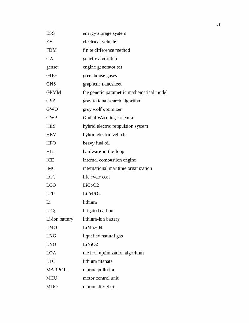
xi
ESS energy storage system
EV electrical vehicle
FDM finite difference method
GA genetic algorithm
genset engine generator set
GHG greenhouse gases
GNS graphene nanosheet
GPMM the generic parametric mathematical model
GSA gravitational search algorithm
GWO grey wolf optimizer
GWP Global Warming Potential
HES hybrid electric propulsion system
HEV hybrid electric vehicle
HFO heavy fuel oil
HIL hardware-in-the-loop
ICE internal combustion engine
IMO international maritime organization
LCC life cycle cost
LCO LiCoO2
LFP LiFePO4
Li lithium
LiC6 litigated carbon
Li-ion battery lithium-ion battery
LMO LiMn2O4
LNG liquefied natural gas
LNO LiNiO2
LOA the lion optimization algorithm
LTO lithium titanate
MARPOL marine pollution
MCU motor control unit
MDO marine diesel oil

xii
ME main engine
MG motor/generator
MGO marine gas oil
MOO multi-objective optimization
MSS the marine systems simulator
NCA Lithium Nickel Cobalt Aluminum Oxide
NFL no free lunch theorem
NG natural gas
NMC Lithium Nickel Manganese Cobalt Oxide
NN neural network
NPV net present value
OCV open circuit voltage
OGV ocean-going vessels
P2D Pseudo 2-dimensional model
PDE partial differential equation
PHES plug-in hybrid electric propulsion system
PM particulate matters
PMC model predictive control
PMP Pontryagin Minimum Principle
PSO particle swarm optimization
PTI power take-in
PTO power take-off
RC resistor-capacitor
RL reinforcement learning
RMSE root-mean-squared error
SA simulated annealing
SCR selective catalytic reduction
SEEMP ship energy efficiency management plan
SEI solid-electrolyte layer
SOC state of charge
SOH state of health

xiii
SPM single particle model
SQP sequential quadratic programming
TOC total ownership cost
UC ultracapacitor
ULSD ultra-low sulphur diesel
UVic University of Victoria

xiv
Nomenclature
𝑄𝑚𝑎𝑥 the maximum capacity of battery
𝑄𝑟𝑎𝑡𝑒𝑑 the rated capacity of battery
𝑉𝑚𝑒𝑎𝑠 measured battery voltage
𝑉𝑠𝑖𝑚 simulated battery voltage
𝑉𝑜𝑐 battery open circuit voltage
𝑅𝑖 battery inner resistance
𝑅1, 𝑅2 resistance in battery RC circuits
𝐶1, 𝐶2 capacitance in battery RC circuits
𝑉𝑖, 𝑉1,𝑉2 the voltage of inner resistance and two RC circuits
𝑉𝑡 terminal voltage (or output voltage)
𝐼 current
𝑡 time
𝑡𝑜 the initial time
𝑡𝑓 the end of time
𝑖 the time step
𝑍 the impedance
𝛼 coefficient of SOC
𝑗𝐿𝑖 microscopic Li ions flow rate
𝛿𝑛, 𝛿𝑝, 𝛿𝑠𝑝 the thickness of negative, positive electrode and separator
𝐴 the electrode surface area
𝛼𝑎, 𝛼𝑐 the anodic and cathodic charge transfer coefficient
𝑎𝑠 the active surface area per electrode unit volume
𝑅 the ideal gas number
𝐹 Faraday’s number
𝜂 overpotential
𝜙𝑠, 𝜙𝑒 the solid and electrolyte potential
𝑈 the equilibrium open circuit potential
𝑐𝑠 ion concentration in solid phase particle

xv
𝑐𝑠,𝑚𝑎𝑥 the maximum solid concentration
𝑗0 the exchange current density at the equilibrium state
𝑘 the reaction rate
𝑐𝑒, 𝑐𝑠𝑒 the ion concentration in the electrolyte and SEI
𝐷𝑠 the solid phase diffusion coefficient
𝑟 the particle radius
𝑐𝑠𝑎𝑣𝑔
the average value of total ions installed in the solid particle
𝑉 the volume of solid particle
𝑆𝑂𝐶 state of charge
𝜃𝑛 the percentage of the actual concentration compared to the
maximum concentration
𝜃100%, 𝜃0% theoretical maximum and minimum concentration percentage
𝐷𝑒𝑒𝑓𝑓
the effective electrolyte phase diffusion coefficient
휀𝑒 the electrolyte phase volume fraction
𝑡0 the transference number
𝑅𝑓 the film resistance inside the cell
𝜙𝑠,𝑝, 𝜙𝑠,n the solid phase potential at the positive electrode (cathode) and
the negative electrode (anode)
𝑄𝑙𝑜𝑠𝑠 battery capacity losses
𝐸𝑎 the activation energy
𝐴, 𝐵 the coefficients in the battery life prediction model
𝑧 the exponent of time in the battery life prediction model
𝑇 temperature
𝐴ℎ battery throughput discharge capacity
N battery cycling numbers
𝐷𝑂𝐷 battery depth of discharge
𝐶𝑟𝑎𝑡𝑒 battery current rate
𝑚𝑓𝑢𝑒𝑙 mass of engine fuel consumption
𝑃𝑒𝑛𝑔,𝑡 the engine power output at time t
𝐵𝑆𝐹𝐶𝑃 the brake specific fuel consumption at corresponded power 𝑃

xvi
𝐸 engine emissions
𝐸𝐹𝑃 the emission factor at power P
𝐸𝐹𝑆𝑂𝑥 the emission factor for SOx
𝑆% the sulphur content of the marine fuel
𝐿𝐶𝐶 life cycle cost
𝐶𝑐𝑎𝑝 capital cost
𝐶𝑜𝑝𝑒 operational cost
𝐶𝑟𝑒𝑠𝑑 residual cost
𝑁𝑃𝑉 net present value
𝐶𝑡 the net cost in year t
𝑁𝑡 total lifetime in year
𝑟 the annual discount rate/inflation rate
𝐶𝑒𝑛𝑔 engine cost
𝐶𝑏𝑢𝑘 bunkering system cost for NG-fueled engines
𝐶𝑒𝑠𝑠 battery ESS cost
𝐶ℎ𝑦𝑏 hybridization and electrification cost
𝐶𝑐ℎ𝑎𝑔 charging facility cost for plug-in hybrid propulsion systems
𝐶𝑟𝑖𝑛 reinvestment cost for battery replacement
𝑃𝑒𝑛𝑔 engine power
𝐸𝑒𝑠𝑠 battery ESS energy
𝑝𝑒𝑛𝑔 price of engine
𝑝𝑒𝑠𝑠 price of battery ESS
𝐿𝑏𝑎𝑡 lifetime of battery
𝑘𝑡 the battery replacement frequency
𝐶𝑒𝑛𝑒𝑟𝑔𝑦 total energy consumption cost
𝐶𝑚𝑎𝑖𝑛𝑡 engine maintenance cost
𝐶𝑓𝑢𝑒𝑙 marine fuel cost
𝑝𝑓𝑢𝑒𝑙 price of marine fuel
𝑚𝑓𝑢𝑒𝑙 total mass of consumed fuel
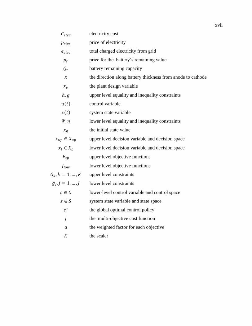
xvii
𝐶𝑒𝑙𝑒𝑐 electricity cost
𝑝𝑒𝑙𝑒𝑐 price of electricity
𝑒𝑒𝑙𝑒𝑐 total charged electricity from grid
𝑝𝑟 price for the battery’s remaining value
𝑄𝑟 battery remaining capacity
𝑥 the direction along battery thickness from anode to cathode
𝑥𝑝 the plant design variable
ℎ, 𝑔 upper level equality and inequality constraints
𝑢(𝑡) control variable
𝑥(𝑡) system state variable
𝛹, 𝜂 lower level equality and inequality constraints
𝑥0 the initial state value
𝑥𝑢𝑝 ∈ 𝑋𝑢𝑝 upper level decision variable and decision space
𝑥𝑙 ∈ 𝑋𝐿 lower level decision variable and decision space
𝐹𝑢𝑝 upper level objective functions
𝑓𝑙𝑜𝑤 lower level objective functions
𝐺𝑘, 𝑘 = 1,… , 𝐾 upper level constraints
𝑔𝑗 , 𝑗 = 1,… , 𝐽 lower level constraints
𝑐 ∈ 𝐶 lower-level control variable and control space
𝑠 ∈ 𝑆 system state variable and state space
𝑐∗ the global optimal control policy
𝐽 the multi-objective cost function
𝑎 the weighted factor for each objective
𝐾 the scaler

xviii
Acknowledgments
I would like to express my sincere gratitude to my supervisor, Prof. Zuomin Dong, for
his close guidance and unremitting support during my PhD journey. His wise and unique
perspectives have inspired me in solving complicated engineering problems on both the
automobile and marine clean transportation research.
I also want to thank all of my colleagues in the UVic clean transportation team for their
valuable advice and discussions, especially Miss. Yuqi Tong for her assistances in
providing and preparing battery experimental data, Dr. Huachao Dong for helping
construct surrogate-model based optimization algorithms, and Anthony Truelove for
sharing marine knowledge and providing valuable editorial advice. I am extremely thankful
to my committee members for their time and effort in reviewing this work.
Finally, I would like to say thank you to my family, without whose support and
encouragement this work would have never been done. I love you all for everything you
have done for me.

xix
Dedication
This dissertation is dedicated to my husband Keda and our daughter Jean. You have
enriched my life.
Chapter 1 Introduction
1.1 Motivation
1.1.1 Background
Today, the marine industry is facing the most challenging emission standards in the
world. Maritime transportation has carried more than 80% of the world trade which emitted
about 2%-3% global CO2, 10%-20% NOx, and various other pollutants [1]. Under the high
pressure of keeping the global average temperature rise below 2ºC above pre-industrial
levels in this century [2], the International Maritime Organization (IMO) has taken a crucial
step and decided to reduce the shipping CO2 to half of their 2008 levels by 2050 [3].
Specifically, the IMO International Convention for the Prevention of Pollution from Ships
(also known as the MARPOL, as an abbreviation of marine pollution) has listed detailed
restrictions for marine pollutions. Annex VI of MARPOL was put into effect on 19 May
2005, with the aim of gradually reducing greenhouse gases (GHG) emissions and harmful
pollutants from ships in defined emission control areas (ECA) [4].
Emissions from increased shipping activities have caused many problems for both the
environment and human health. More stringent regulations have been made by IMO to
restrict specific air contaminants emitted by near shore ship operations in the ECAs to
avoid harmful impacts for humans. Those specific contaminants include sulphur oxides
(SOx, including mostly SO2 and some SO), nitrogen oxides (NOx, include NO2 and NO,)
and particulate matters (PM), all of which can cause potential heart diseases, lung diseases
and cancer. The restriction of SOx emissions is achieved by limiting the sulphur content of
the fuel oils used in both main and auxiliary engines onboard. Currently, the sulphur
content in marine fuels used in ECAs is limited to 0.1% (i.e. 1000 ppm), which is 35 times

2
lower than that of outside ECAs. The NOx emission from ship engines larger than 130kW
must meet required limits corresponding to its construction date and engine speed. New
ships built after 2016 are restricted to emit NOx between 2 and 3.4 g/kWh accoring to the
engine speed, which is about 5 times lower than engines built before 2000. The energy
efficiency design index (EEDI) and ship energy efficiency management plan (SEEMP) are
adopted to encourage ship operators to improve ship efficiency and reduce emissions by
employing new technologies [5].
The west coast region of Canada has very prosperous shipping activities among various
islands in British Columbia (BC). As one of the largest passenger ferry companies in the
world, BC Ferries owns 47 ports of call and operates more than 500 sailings every day in
BC, providing necessary transportation services and feeder services to different island
communities. The Port of Vancouver is the largest port in Canada, facilitating 27 major
marine cargo terminals which receive over 3,100 ocean-going vessels (OGVs) every year
[6]. It has been reported in Canada’s Air Pollutant Emission Inventory [7] that ship-emitted
SOx and NOx are the main contributors in the transportation sector of BC. The activities of
shipping near the coastal area of BC are within ECAs and must obey the emission standards
issued by IMO.
Under such conditions, this research intends to design a more environmentally friendly
solution for the marine industry, based on the collaboration project between the University
of Victoria (UVic) and some ship companies in BC, Canada. Recently, various solutions
have been proposed to reduce marine emissions, which can be categorized into three main
strategies: (i) using low sulphur content fuels; (ii) using after-treatment technologies for
exhausted gases; (iii) adopting new technologies such as hybrid and electric propulsions.

3
First, low-sulphur distillate oils currently used in the ship industry include marine diesel
oil (MDO) and marine gas oil (MGO). The convention marine fuel is the heavy fuel oil
(HFO, also known as residual fuel oil) and has 3.5% sulphur content. The MGO lowers
this value to about 0.1% that can greatly reduce total SOx emissions. Moreover, vessels
operating on the inland waters of Canada and The United States are required to use ultra-
low sulphur diesel (ULSD), which has a sulphur content of only 0.0015% (or 15 ppm) [8].
However, the lower the sulphur content, the more expensive the fuel cost. The price of
MGO is more than double that of HFO, increasing about $11 CAD per cargo tonne [9]. As
such, liquefied natural gas (LNG) has become more and more popular in the marine
industry due to its negligible sulphur content and lower price. Many groups have conducted
feasibility studies into using LNG-fueled vessels, and have investigated the perspectives
and challenges with respect to the legal, economic and technological factors [10, 11]. More
and more LNG-fueled vessels are operating worldwide, with reported lower CO2 emissions
and less operational cost [12].
Second, the after-treatment of exhausted gas has been widely adopted to reduce heavy
emissions, especially in those conventional vessels using cheap and dirty HFO. Ships can
install scrubbers to reduce SOx and PM, and use selective catalytic reduction (SCR) or
exhaust gas recirculation (EGR) for NOx cleaning. The combination of using scrubbers
with SCR or EGR provides an effective solution to fulfil the emission requirements in
ECAs. The main advantage of using after-treatment technologies is that it can cooperate
with the existing fuel system to meet emission standards and use cheap fuels. However, it
also increases the investment cost for installing and maintaining the equipment.

4
Third, hybridization and electrification technologies have been used in ship propulsion
systems to improve efficiency and reduce carbon emissions. These systems involve
additional cleaner power sources and provide more flexible configurations. By
disconnecting the engines with the propellers, main engines can operate at higher efficiency
area when needed, and store surplus energy in rechargeable energy storage system (ESS).
Renewable energy technologies, such as rechargeable battery ESS, ultracapacitor (UC),
fuel cell, and flywheel, have been deeply examined as potential prime movers [13]. Among
them, lithium-ion (Li-ion) battery ESS presents as the most promising technology
considering energy density, cost, and reliability. The hybrid configuration of powertrain
systems enables more flexible control and higher operational efficiency [14]. Unlike
conventional mechanical propulsions that only use internal combustion engines (ICE),
hybrid powertrain systems adopt a rechargeable battery ESS and electric motors to partially
or fully substitute ICE in certain conditions. Preliminary studies of applying hybrid electric
technology to different vessels have shown great emissions reductions and fuel savings
compared to the original ones [15-17].
Among the aforementioned possible solutions to solve ship emission problems, taking
hybrid electric technology and using low-sulphur content marine fuels appear more
attractive. The cost and performance evaluation of using NG-fueled engines versus ULSD-
fueled engines is currently a hot topic in the marine industry. Moreover, there have been
many successful experiences in the automotive industry with using hybrid technologies to
substitute conventional vehicles, which can be adopted to benefit the marine industry as
well. However, the flexibility of hybrid powertrain systems raises additional difficulties in
system design and optimal energy management. The special characteristics of Li-ion

5
batteries require advanced control logics and induce uncertain performance degradation
during usage. It is therefore of great interest to investigate the design and control of hybrid
electric marine propulsions with Li-ion battery ESS, and compare the performance of using
NG-fueled engines vs. diesel engines.
1.1.2 General Review
Hybridization and electrification are considered effective methods to improve system
efficiency and reduce emissions from both land- and water- based transportations [18, 19].
Hybrid electric powertrain systems normally include an ICE, a large battery ESS, electric
machines (generators and motors) and power electronics[19]. Commonly used hybrid
powertrain configurations can be classified into series, parallel, and series-parallel (or
power-split) hybrid systems [20]. Depending on their configurations, various gear sets and
gear reductions may also be needed. All electric ships are also achievable if an integrated
electric power system is built so that all the energy in hybrid configurations is transferred
into electricity. The application of hybrid marine propulsion systems has been reviewed in
many studies [19, 21, 22]. In conclusion, the main advantages include
providing more flexible operation;
increasing the system redundancy;
improving engine fuel economy by optimizing its operation conditions;
reducing fuel consumption and air emissions;
canceling auxiliary engine generator sets (Genset) by providing electricity via ESS;
reducing engine operational time and maintenance cost.
In hybrid marine propulsion system design, the main challenges are the component sizing
and the energy management of the main power sources–engine and battery ESS. The

6
design of other components, such as electric machines and power electronic converters,
are directly related to these two components.
NG-fueled engines create both opportunities and challenges for the marine industry. As
discussed, LNG is a clean and non-sulphur fuel. Exhausted emissions such as SOx and NOx
can be negligible if using LNG engines. Natural gas consists of more than 90% of methane
(CH4). The high hydrogen to carbon ratio of CH4 implies lower CO2 emissions and higher
water vapor. Changing engine fuel from diesel to natural gas can significantly reduce GHG
emissions and air pollutants [23]. When natural gas is cooled to -162ºC, LNG is obtained
with only 1/600th volume compared to the original gas. LNG is more favorable in
transportation due to its reduced gas volume, which makes it efficient to store and transport.
NG-fueled engines normally can be categorized as dual-fueled (with diesel pilot)
compression-ignition engines and lean-burn spark-ignition engines. Dual-fueled LNG
engines have more flexibility to use either natural gas or diesel fuel. Suppliers such as
Wärtsilä and MAN have developed mature dual-fueled LNG engines. Lean-burn ignited
LNG engines use a spark plug to ignite the natural gas/air mixture. Their suppliers include
Rolls-Royce and Mitsubishi. Currently, there are 76 LNG-fueled vessels in operation
worldwide (excluding LNG carriers) [24]. Ship companies in Canada are on the leading
edge of transferring their vessels to LNG-fueled ones. BC Ferries has updated two of the
548-foot-long Spirit-class ferries to LNG-fueled vessels. They also adopted three new
Salish-class ferries that are capable of running duel-fuel (either LNG or ULSD). Robert
Allan Ltd. has developed LNG-fueled (and LNG-diesel dual-fueled) escort tugs with
powerful bollard pulls [12]. Several studies have discussed the environmental and
economic benefits of using NG-fueled engines in different types of ships [11, 25, 26].

7
However, these studies are all based on conventional vessels with mechanical propulsion
systems. It is of great interest to discover the potential benefits of adopting NG-fueled
engines in hybrid marine propulsions.
Li-ion batteries are the most widely applied type of ESS in hybrid powertrain systems
with outstanding performance of energy and power density. They are also called “rocking-
chair” batteries due to the nature of transferring, instead of consuming, the Li ions between
the anode and cathode during charging and discharging processes. Even though the price
of Li-ion batteries has considerably decreased in recent years, it is still very expensive
compared to engines and other electrical machines[27]. Another critical problem of using
Li-ion battery ESS under high power demand is the aging phenomenon caused by
irreversible microscopic electrochemical reactions inside each single battery cell [28].
Materials, manufacturing, operating temperatures and other conditions can affect battery
deterioration rates [29]. The performance degradation of batteries would induce capacity
decay and impedance increment, eventually reducing their lifetime. In general, Li-ion
battery ESS tends to have a much lower lifetime than other components (such as engines,
electric machines) in hybrid powertrain systems. The requirement of replacing a battery
pack would aggravate its total ownership cost. A better understanding of the battery aging
process can be critical to avoid its deterioration and prolong its lifetime.
It is an urgent need to develop an accurate battery model that can quantitatively analyze
its performance deterioration rate and support hybrid powertrain system design. Battery
performance degradation and life heavily depend upon the actual use pattern and operating
temperature. The control algorithm of hybrid systems plays an important role in extending
battery lifetime by avoiding harsh charging and discharging at high current rate. An
8
accurate Li-ion battery model is crucial in developing optimal energy management
system. Three main types of modelling methods are mostly used in the literature [30-32]:
the empirical model, the equivalent circuit model, and the electrochemical model (or
“Doyle-Fuller-Newman” model [32]). Depending on complexity, accuracy and
computational time, these models have been used for different purposes. A more specific
review on battery modelling methods will be discussed in Chapter 2.
The integrated design and control of hybrid electric powertrain systems are complicated
problems. For power systems with only one type of energy source, such as pure mechanical
or pure electric architecture, there is no possibility to develop an advanced energy
management strategy. Hybrid propulsion systems, on the other hand, offer more freedom
for power control due to the increased additional power source. Therefore, the intelligent
control strategy must be decided in the energy management system to take optimal
decisions of power distribution between the engine and battery ESS. Heuristic-based and
optimization-based control strategies have been deeply investigated in the automotive
industry for hybrid electric vehicles. However, the marine industry still lacks sufficient
study of optimal control for hybrid propulsions. Most hybrid vessels take a rule-based
control strategy [33, 34]. A few investigated the equivalent consumption minimization
strategy (ECMS) for optimal hybrid tugboat control [35]. Moreover, previous studies of
hybrid marine propulsions[14, 19] [33-35], to the best of the author’s knowledge, did not
consider the combined system design and control optimization.
The integrated design and control optimization of hybrid marine propulsions must solve
the component sizing optimization and energy management strategy optimization
simultaneously in its searching algorithm. Most studies on hybrid electric vehicle (HEV)

9
design focused on optimal component sizing with pre-determined control rules [36], then
find the global optimal control strategy based on selected (not necessarily optimized)
power components [37]. The problem complexity can be greatly increased when
encountering two jointed intricate optimization problems. Fathy, et al. [38] discussed the
combined plant and controller design optimization problem on coupled conditions, in
which the nested and simultaneous optimization strategies are proven to find the global
optimum. In recent years, more and more studies take a step forward to solve the combined
hybrid powertrain system component design and control in a nested framework, with the
top level optimizing component sizes and the bottom level searching for the optimal control
rules [39, 40]. It is therefore a great time to examine the possibilities of solving the
integrated hybrid propulsion system design and control optimization for marine
applications.
It is usually computationally expensive to solve the complex integrated design and
control optimization problems. Population- and/or evolutionary-based heuristic
optimization algorithms are commonly adopted to solve the design problem, such as
particle swarm optimization [41], genetic algorithm [42]. The model-based optimal control
strategies for both on-line and off-line implementations in a PHEV are discussed in [20].
It is usually cost a heavy computational burden in searching for global optimal control
rules. For those types of work, a surrogate model (or meta-model) can be developed as an
approximation of the actual simulation model with reduced computational time.
Commonly used metamodeling techniques in building surrogate models, including the
experimental design (or sampling methods), different types of surrogate models, and model
fitting methods will be discussed in Chapter 4.

10
Given these circumstances, this study is motivated to develop a methodology to
effectively solve the combined design and control optimization for hybrid electric marine
propulsions in a bi-level, nested approach, discovering all potential benefits of using NG-
fueled engines and Li-ion battery ESS. The model-based design and optimization method
is introduced to support the hybrid propulsion design with detailed engine efficiency and
emission models, proposed battery performance degradation model and developed hybrid
energy management system model.
1.2 Define Research Goals
The main goal of this dissertation is to identify the challenges and solve the problems in
optimal hybrid marine propulsion system design and control. Meanwhile, this dissertation
fills the gap in modelling Li-ion batteries in the marine industry by adopting advanced
mathematical models of electrochemical batteries to demonstrate their performance
degradation. Finally, it draws on the experiences of hybrid powertrain system design from
the automotive industry and optimization methodologies from the optimization community
to solve the design and control problems. This involves hybrid propulsion system design,
modelling and sizing of the key components, and the development of optimal hybrid
system control strategies. The system design, in this dissertation, refers to the dimensioning
of key components in hybrid propulsions. The control strategy of hybrid systems means
properly distributing the power demands to different power sources to achieve less fuel
consumption and emissions. The most challenging part is that the optimization of hybrid
system design is coupled with the optimal control strategy development. Therefore,
advanced optimization algorithms must be adopted to solve this problem. The optimized
hybrid systems should obtain the best economic and environmental benefits.

11
In the marine industry, the propulsion system design still heavily rely on the
engineering experiences due to the lack of model-based design and optimization tools. The
performance degradation of Li-ion battery obviously aggravates this situation, making the
sizing of battery ESS even more difficult. Therefore, this research develops an integrated
hybrid marine propulsion system design platform with accurate battery performance
degradation and life prediction model. It can support optimal design and control by
reflecting all the economic impacts, including the initial investment cost (affected by the
component design) and operational cost (affected by control decisions), to the ultimate total
life cycle cost (LCC). Moreover, advance algorithms from optimization community are
introduced and discussed in solving the intricate complex design and control optimization
of hybrid propulsion systems. Surrogate model-based optimization methods are adopted to
improve computational efficiency.
To summarize, the research goals in this dissertation include:
build an accurate Li-ion battery performance degradation and life prediction model
to support optimal energy management in hybrid powertrain systems;
develop an integrated ship modelling platform that can support the design and control
of hybrid marine propulsion systems;
build the life cycle cost (LCC) model of hybrid ship propulsions to reflect the
economic variations of powertrain hybridization and electrification;
formulate the combined hybrid plant design and control problems as an integrated
optimization problem;
find an efficient global optimization algorithm to solve the complex optimization
problem;

12
implement proposed methodology on a real marine vessel to find the optimal
hybrid propulsion system design.
1.3 Dissertation Organization
The arrangement of this dissertation is organized as follows. Chapter 2 develops a Li-ion
battery performance degradation and life prediction model based on acquired experimental
data. Chapter 3 discusses the detailed component models and control strategies of hybrid
marine propulsion systems based on the integrated ship simulation platform. A LCC model
of hybrid propulsions is also developed in this chapter based on collected price information
for ships operating in BC, Canada. Chapter 4 proposes a surrogate model-based global
optimization framework to solve the nested co-design optimization problem for hybrid
propulsion system design and control. The proposed method is implemented for a harbour
tugboat design case study. Chapter 5 draws conclusions and outlooks of this research.

13
Chapter 2 Li-ion Battery Performance Degradation Modelling
Li-ion batteries have been widely used in hybrid powertrain systems because of their
extraordinary performances, massive production capability, and matured manufacturing
technology. However, challenges remain in the battery cost and its performance
degradation phenomena. The inevitable aging process of battery during usage will not only
reduce its designed capacity, but also increase cost for maintenance and replacement. This
problem will be severer in hybrid marine systems since it has much higher capacity of
battery ESS than other applications (e.g., HEVs). The appropriate sizing of the battery ESS
and the energy management/power control strategies depend upon the accurate prediction
of battery degradation under the specific use pattern – the foundation of powertrain system
design and control optimization. In this chapter, a systematical review is presented to
conclude the main degradation mechanisms and relevant affecting factors. A battery
performance degradation and life prediction model is developed and verified using
acquired experimental data.
2.1. Review on Battery Degradation Mechanisms
The characteristics of metallic Li enable high energy and power density of Li-ion
batteries [43]. The performance and degradation mechanisms of different types of Li-ion
battery are highly related to the materials used in the cathode, anode, and electrolyte.
Therefore a good understanding on available commercial materials and their characteristics
is important for further modelling works.

14
2.1.1 Li-ion Battery Materials
Anode Materials
The most commonly used anode material in commercial Li-ion batteries is litigated
carbon (LiC6). Carbon material has abundant natural reserve volume therefore can offer
very low price for the market. This layered crystal compound is very stable during ion’s
intercalating processes, providing great cycling performance. Moreover, the overpotential
of LiC6 is about 0.5V vs. Li/Li+, which can help construct a high battery overall voltage
(usually between 3 and 4.5V, depending on the cathode material). However, it has only
372 mAh/g theoretical energy density, much less than metal Li (3860 mAh/g). Therefore,
LiC6 is not very competitive in providing high energy density battery.
Lithium titanate (LTO) is another type of anode material developed in recent years. It
can provide longer cycling lifetime and has higher tolerance of large current rate compared
to LiC6. With negligible volume change during Li ions’ intercalation, LTO has excellent
cycling performance [44]. The overpotential of LTO anode is about 1.55V against Li/Li+,
which is about 3 times higher than LiC6. This high equilibrium potential has both pros and
cons, it can help avoid the formation and growth of anode solid-electrolyte layer (SEI) and
reduce capacity losses, but also lower the overall battery voltage (to about 2.4V, depending
on the cathode material). The theoretical capacity of LTO is only half of graphite anode
(about 170 mAh/g) thus also hard to achieve high energy density.
There are many other advanced anode materials under development and not yet
commercialized, such as metallic Li anode, graphene nanosheet anode, Si-based alloy
anode, etc.

15
Metal Li could be an ideal choice as the anode material , because (i) it is the lightest
metal element and offers the lowest density (0.534 g/cm3), which are favorable for high
energy density; (ii) it has the lowest reduction voltage (-3.04V vs. standard hydrogen
electrode), allowing the battery to achieve a high potential. However, the
charging/discharging processes can cause severe dendrite growth on the metallic Li. This
poses risks in inducing battery inner short-circuit and other safety issues. It also has poor
cycle performance and low Columbic efficiency. Although there has been some
improvements on the stable cycling performance of lithium mental anode [45], it is hard to
see its commercialization in the near future.
Graphene has been known as the thinnest and lightest compound, which are favorable
for achieving high energy density. It also has the strongest mechanic structure and great
electric conductivity. Graphene nanosheet (GNS) can provide large reaction surface areas
and a stable structure as the anode material of Li-ion battery. GNS can improve the battery
capacity and energy density through merging nanomaterials into the graphene [46, 47], but
the cyclic performances and safety issues are still unsolved problems.
Silicon (Si) based anode has drawn the most attention in recent years because of its
abundance, performance, and non-toxicity characteristics. It has 10 times more specific
capacity than carbon-based anodes, which can provide extremely high volumetric and
gravimetric capacity. However, it also has poor cyclability due to the large volume change
of Si during the Li ions intercalations [48]. The nanostructured Si anode can potentially
avoid the severe volume expansion. Different nanostructure design, such as nanowires,
hollow nanostructures, and clamped hollow structures, have been showed in [49].

16
The ideal anode material should have high capacity, low potential against Li/Li+, long
lifetime, and low cost. Considering these factors, the most commonly used materials and
most promising materials in the future have been compared in Table 1.
Table 1: Comparison of Anode Materials
C LTO Li Si
Specific Capacity
(theoretical) (mAh/g)
[50]
372 175 3862 4200
Potential vs. Li (V)
[50] 0.05 1.55 0 0.4
Volume Change (%) 12% 1% 100% 420%
Density (𝑔/𝑐𝑚3) 2.25 3.5 0.53 2.3
Advantages
• low cost;
• good cycle
performance;
• long lifetime;
• high cycle rate;
• high energy
density;
• high voltage;
• high energy
density;
Disadvantages • low energy
density
• high cost;
• low voltage;
• low energy density;
• dendrite growth; • high volume
expansion;
Cathode Materials
The cathode materials used in Li-ion batteries include a variety of lithium metal oxide
compounds, such as the Lithium Ion Phosphate (LFP), Lithium Cobalt Oxide (LCO),
Lithium Nickel Manganese Cobalt Oxide (NMC), Lithium Nickel Cobalt Aluminum Oxide
(NCA), and so on. The application of these different materials highly depends on their
energy density, voltage, safety, cost and many other factors [43, 48, 51].
LiCoO2 (or LCO) is one of the earliest commercialized cathode materials. It has very
high theoretical specific capacity and can provide high voltage [43, 52-54]. The major issue
of LCO is its low thermal stability due to the layered structure. Thermal runaway can be
observed at about 200ºC, where exothermic reaction happens between released oxygen
from LCO and other organic materials in the battery. The high cost of Co is also a concern

17
for the large-scale application. Structure distortion and deterioration of LCO can be
observed under high cycle currents.
LiNiO2 (or LNO) has similar characteristics of LCO, which also has layered structure
and high specific energy capacity (about 275mAh/g in theory and 150mAh/g in practice).
The synthesis process of LNO usually gains over-stoichiometric phases of extra Ni ions,
hence, introduces unstable factors and causes low stability, poor cycling performance and
rapid capacity fading.
LiMnO2 (or LMO) battery, compared to the layered structure of LNO and LCO, is well
known for its three-dimensional spinel structure that is easily for ions’ insertion and
extraction. The excellent reversibility inside spinel LMO makes its practical specific
capacity almost the same as LNO and LCO, even though its theoretical capacity is only
half of them. The advantages also include lower internal resistance, safer thermal stability,
cheap cost and non-toxicity for environment. Drawbacks include low specific energy
density, materials dissolution upon cycling, and poor cycle life.
LiFePO4 (or LFP) has an olivine structure, which is very stable and can provide superior
cycling performance. The strong bonding of oxygen in phosphate group makes it stable to
resist thermal runaway, thus, have a safe performance at high temperature. However, the
theoretical specific capacity is not very high. It also has a flat potential platform of 3.4V
vs. Li/Li+. LFP has been largely used in electrical vehicles (EVs) and HEVs in the
automotive industry.
To gain all the strengths from LNO, LMO and LCO, a combination of these three has
been invented. Ni-based materials have higher energy density, low cost, and longer lifetime
than Co-based ones. Mn-based systems benefit from the spinel structure and can achieve a

18
low internal resistance and high voltage. Doping small amount of Co, Mn or Al into Ni-
based materials can greatly improve the overall performances and gain all the advantages.
The combinations of these metals are able to provide high energy and power density with
the stable thermal behavior. LiNiMnCoO2 (or NMC) and LiNiCoAlO2 (or NCA) are two
recently commercialized and widely used cathode materials in Li-ion batteries. They have
been gradually substituting conventional LFP or LCO in the hybrid powertrain systems in
transportation area. The property of NMC-type battery is determined by the proportion of
Ni, Mn and Co in its mixture. Usually the common proportions are NMC(1:1:1),
NMC(5:3:2), NMC(6:2:2) , or NMC(8:1:1) [50]. The trend is to reduce the usage of
expensive material Co and increase the proportion of Ni to have a lower price.
NMC and NCA are both Ni-based material with high specific energy, low internal
resistance, and long lifetime. They have similar characteristics. Normally the proportion of
Al in NCA is very small, such as the LiNi0.8Co0.15Al0.05O2. NCA is reported to have higher
specific capacity (about 300Wh/kg), however, it can have unstable thermal behavior at
elevated temperatures. Battery manufacturers are producing NMC and NCA based on their
own considerations. For example, LG Chemicals has cooperated with General Motors to
provide batteries for their EVs with NMC811, NMC622, and NMC712 types of Li-ion
batteries. Panasonic, on the other hand, produces NCA type of batteries for Tesla EVs.
Battery manufacturers who produce NMC batteries include (but not limited to) LG
Chemicals, Samsung SDI, SK Innovation, CATL, etc. Generally, NMC811 cathode is
reported to have greater cycle life and lower cost than NCA.
Conversion cathode materials, such as fluorine and chlorine compounds, sulfur and
lithium sulfide, or selenium, usually have high theoretical specific and volumetric

19
capacities. However, they normally suffer from poor cycling performance, large volume
expansion and unwanted side reactions [48]. These type of materials have not yet been
commercialized; therefore, will not be considered in the application of hybrid powertrain
system design.
The comparisons of these commercialized cathode materials have been showed in Table
2. Recent studies on advanced battery materials showed that the NMC-based cathode and
silicon alloy-based anode will be the most promising type of Li-ion batteries with higher
energy density and decreased cost [50]. However, the LFP cathode with carbon-based
anode battery is still one of the most popular types of battery at present, mainly because of
its superior safety performance. LFP battery has been widely applied in many HEVs and
EVs, therefore, it was tested and measured to help construct battery performance
degradation model in this study.
Table 2: Comparison of Commercialized Cathode Materials
LiMn2O4
(LMO)
LiFePO4
(LFP)
LiCoO2
(LCO) NMC NCA
Theoretical
Specific Capacity
(mAh/g)[48]
148 170 274 280 279
Average Voltage
(V) [48] 4.1 3.4 3.8 3.7 3.7
Structure Spinel Olivine Layered Layered Layered
Lifetime * *** ** *** **
Cost [50] * ** ** *** ***
Advantages
• high
thermal
stability;
• high
safety;
• high
capacity;
• high energy/power density;
• long lifetime;
• low internal resistance;
• low cost;
Disadvantages
• low
capacity;
• low
lifetime;
• low
energy
density;
• poor
stability;
• high cost;
• low thermal stability at high
temperature;
• NMC811 has higher cycle life and
lower cost than NCA;

20
Electrolytes in Li-ion batteries play an important factor to build stable electrochemical
windows for battery reductions and oxidations. Commercial electrolytes normally include
organic solvents, Li salts and some additives. Experiments have showed that the stable
voltage range of the liquid electrolyte is from 0.8V to 4.5V vs. Li/Li+. Apparently, the most
widely used carbon-based anodes (0.5V vs. Li/Li+) are outside this range. Hence,
electrochemical reactions will happen between carbon-based anodes and organic solvents
spontaneously and form a solid-electrolyte interface (SEI) along the active anode surface.
After the SEI is built up, it acts as a barrier to stop further corrosions from electrolytes. The
SEI formation and growth can greatly affect battery performance degradation. On the one
hand, the SEI can protect the active anode material and facilitate more stable cycling
performance. On the other hand, it also consumes cyclable ions and increases the
impedance, which deteriorates the cell performance. This characteristic of SEI is the unique
feature of using carbon-based anode material.
2.1.2 Battery Performance Degradation Mechanisms
The performance deterioration of Li-ion batteries is an inevitable process due to the
irreversible electrochemical side reactions. Temperature, current, and battery state of
charge (SOC) are all relevant to the degradation rate. Depending on if the battery is in a
working or storage situation, the degradation mechanisms perform differently on the anode
and cathode materials.
Cyclic capacity decay starts right after the first charge/discharge process. As discussed,
the formation of SEI on the anode surface not only consumes available ions but also
increases battery inner resistance. A sharp capacity decay can be observed at the negative
electrode at the beginning of battery life [55]. To solve this problem, usually more than

21
adequate Li ions and carbon materials are provided to improve overall cycling
efficiency. However, extra anode material on the negative electrode makes battery
performance limited by the positive electrode. Bourlot, et al. [56] compared fresh batteries
with 1.5 years-aged ones and showed that the SEI layer on negative electrode stayed
relatively stable while binder dissolutions and active metal Li were found on positive
electrodes, which implies positive electrode limited cycling performance. Furthermore,
constantly periodic cycling may aggravate this situation, causing SEI layer becoming
harder and thicker. Ramadass, et al. [31] showed the battery film resistance increases with
the cycling numbers. The losses of available lithium ions are the main reason for cyclic
capacity decay. The study in [57] showed that battery cyclic capacity fading has a direct
link with the thickness of SEI layer. Moreover, microscopic side reactions happen all the
time and cause compound structure deformation, active materials wearing and many other
damages to battery materials [56].
Many factors can affect battery cyclic performance deterioration. Temperature is the
most important one. When battery is cycled at the elevated temperature (e.g., higher than
40 ºC), it can cause structure exfoliations of cathode materials [58]. If a battery is charged
at low temperature (e.g., less than -20ºC), it can cause metal Li plating along the anode
materials. The formation of dendritic Li not only decreases battery capacity but also
induces potential risks of inner short circuit [59]. The charge and discharge current rate (C-
rate) is another important factor. A 1C discharge rate means all the energy inside a battery
can be completely released in 1 hour. If battery is discharged at higher current rates, large
amounts of Li ions will accumulate on the anode surface in a short time. If the diffusion
process of ion is restricted (or limited by the characteristics of battery materials), dendrite

22
Li might be generated. Low C-rate, on the other hand, is more favorable for a safer
performance and longer life. The battery SOC indicates the percentage of remaining energy
that battery can release compared to the rated capacity. The variation of SOC in a cycle,
sometime referred as the depth of discharge (DOD), can also affect battery cyclic
performance. The higher the DOD, the more throughput capacity the battery has to provide.
In another word, higher DOD means harsher usage of the battery therefore can accelerate
the degradation [60].
When battery is in storage or on the rest, chemical reactions still happen due to the
thermodynamic instability of battery materials. Side reactions, mainly on negative
electrode due to spontaneous reactions between the LiC6 and electrolyte, are believed to be
the main reason of calendar life fading [6]. The reaction rate and intensity are highly related
to material properties, storage temperature, and battery open circuit voltage (OCV). The
OCV is determined by the distribution of ions on the cathode and anode; therefore, it has a
direct connection with battery SOC. If the battery is stored at a higher temperature, it will
facilitate secondary reactions and speed up the corrosions [61]. Mild or low temperatures,
on the other hand, can depress the reaction. In general, the storage temperature is more
critical than storage voltage (or SOC) level for calendar life degradation [61].
In conclusion, the main consequences of battery performance degradation include the
capacity decay and impedance increment. The capacity decay is mostly due to the SEI
formation on the anode and side reactions on the cathode, while the battery impedance can
be affected by the material disordering and decomposition as well as the formation of SEI.
Specifically, main reasons for carbon-based anode deterioration are SEI formation and
growth, corrosion of active carbons, lithium metal plating at low temperatures or high rate

23
currents, etc. As for lithium metal oxide cathodes, wearing of active materials,
compound structure changings, and electrolyte dissolving are relevant to the performance
decay. Generally, cyclic aging is much severer than storage aging. To reflect all the
influences by the former discussed factors, battery capacity losses (𝑄𝑙𝑜𝑠𝑠) can be expressed
as a function of current rate (𝐶𝑟𝑎𝑡𝑒), 𝐷𝑂𝐷, temperature (𝑇) and total operational time (𝑡).
𝑄𝑙𝑜𝑠𝑠 = 𝑓(𝐶𝑟𝑎𝑡𝑒 , 𝐷𝑂𝐷, , 𝑇, 𝑡) (1)
2.2. Battery Performance Degradation and Life Prediction Model
Based on the previous discussions, a battery performance degradation and life prediction
model is proposed in this section to capture the battery dynamic behaviors and reflect the
deterioration rate. In which, the performance model calculates battery voltage, SOC, and
other characteristics in each charge/discharge cycle. The life prediction model estimates
the accumulated performance deterioration based on historical usages and gives a
prediction of remaining lifetime under given load profiles.
Different modelling methods are discussed in this section, including previously
mentioned equivalent circuit model, the electrochemical impedance spectroscopy model,
single particle model, and empirical model. The battery performance degradation model is
developed and validated by the 18Ah LiFePO4 battery cycle-life tests. As discussed in
previous section, LiFePO4 has superior safe performance especially at elevated
temperatures, therefore, has been widely used in many hybrid powertrain systems. And it
can certainly be used in the marine industry due to its lower price and good cycling
performance.

24
2.2.1 Li-ion Battery Cycle-life Experiment Data
The specifications of tested LiFePO4 battery are listed in Table 3. This commercialized
battery was purchased and tested in the State-assigned Electric Vehicle Power Battery
Testing Center in Beijing, China.
Table 3: LiFePO4 Battery Specification
Rated Voltage 3.2V
Capacity 18 Ah
Weight Energy Density 120 Wh/kg
Charge/Discharge Cut-off Voltage 3.6V/2.5V
Standard/Fast Charge Current Rate 1C/2C
Continuous/Max. Discharge Currant Rate 3C/15C
The open circuit voltages (𝑉𝑜𝑐) of this battery under charge and discharge conditions are
plotted in Figure 1.
Figure 1: Battery Charge and Discharge Open Circuit Voltage
The main purpose of battery cycle-life tests is to measure battery performance
degradation characteristics through constant periodically cycling. Specifically, the battery
1.5
2
2.5
3
3.5
4
0 0.2 0.4 0.6 0.8 1
Vo
ltag
e (V
)
SOC
Voc_charge
Voc_discharge

25
is charged and discharged under pre-defined current profiles repeatedly and its voltage,
total charging energy and discharged energy are measured. When its capacity reduces to
the 80% of normal capacity, it is recognized as a dead battery and is not suitable for further
usage in transportation application. The cycle-life experiments can be divided into two
groups:
cycling tests: battery is charged at 1C and discharged at 2C
capacity tests: battery is charge and discharged at 1/3C
Cycling tests and capacity tests serve different purposes, thus, having distinct cycling
profiles. Cycling tests are usually under higher C-rate to save experimental time. To fully
measure the available battery capacity, capacity tests were performed after every 25 cycles
under slow charge/discharge process. The cycle-life test profile is showed in Figure 2.
Figure 2: Li-ion Battery Cycle-life Test Profile
The charging protocol is the standard constant current-constant voltage method (CC-
CV). For the capacity test, the battery is charged at 1/3C current rate until it reaches the
maximum voltage (which is 3.6V in this case). Then it will change to the constant voltage
charge at the maximum voltage until the charging current reaches to 0A. The discharging
0
0.5
1
1.5
2
2.5
3
3.5
4
-40
-30
-20
-10
0
10
20
30
0 5,000 10,000 15,000 20,000 25,000 30,000
Vo
lt(V
)
I(A
)
time(s)
Li-ion Battery Cycle-life Test Profiles
I_cycling test (A)
I_capacity test (A)
V_cycling test(V)
V_capacity test(V)

26
protocol is much simpler. The battery is discharged constantly at designed current rate
until its voltage reaches to the cut-off voltage (in this case 2.5V). To ensure a safety testing
environment, the battery was placed in an environmental chamber at 20ºC.
It is quite time consuming to perform thousands of such cycling tests. So far, it has been
cycled about 2000 times and some of the representative curves are plotted in Figure 3.
Figure 3: Battery Cycling Curves
Two significant features can be observed from the curves showed in Figure 3. First is the
reduced experimental time when the cycling number increases. This indicates that the
maximum capacity (𝑄𝑚𝑎𝑥) is decreased thus less energy can be put into the battery. The
second feature is the variation of measured battery voltage in different cycles. Under the
same charge/discharge protocol, the voltage can only be influenced by the battery inner
resistance and/or capacitance. The measurement data have clearly led the conclusions that
have been discussed in the previous section: the performance degradation can cause
capacity decay and resistance increment.
2.4
2.6
2.8
3
3.2
3.4
3.6
3.8
0 5000 10000 15000 20000 25000
Mea
sure
d V
olt
age
(V)
time (s)
Cycle 1
Cycle 500
Cycle 1000
Cycle 1300
Cycle 1500
Cycle 2000

27
The measured battery capacity also verifies the deterioration when the cycling number
increases, as showed in Figure 4.
Figure 4: Measured Battery Capacity in Different Cycles
These acquired battery data will be used to build the battery performance degradation
model. 80% of the measured voltages under charge/discharge current profile are used to
build battery performance model and obtain model parameters’ value, while the rests are
used for validation. Different battery modelling methods have been compared in this study.
The simulated battery voltage from developed battery models has to be validated to find
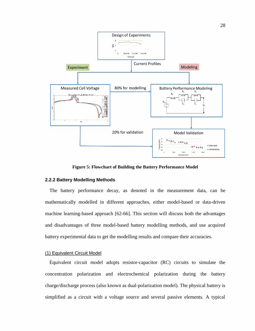
the most appropriate model for the hybrid system design and modelling. The flowchart of
battery modelling and validation process is presented in Figure 5.
0%
20%
40%
60%
80%
100%
120%
0 500 1000 1500 2000 2500
Cap
acit
y R
eten
tio
n (
%)
Cycle Number
28
Figure 5: Flowchart of Building the Battery Performance Model
2.2.2 Battery Modelling Methods
The battery performance decay, as denoted in the measurement data, can be
mathematically modelled in different approaches, either model-based or data-driven
machine learning-based approach [62-66]. This section will discuss both the advantages
and disadvantages of three model-based battery modelling methods, and use acquired
battery experimental data to get the modelling results and compare their accuracies.
(1) Equivalent Circuit Model
Equivalent circuit model adopts resistor-capacitor (RC) circuits to simulate the
concentration polarization and electrochemical polarization during the battery
charge/discharge process (also known as dual-polarization model). The physical battery is
simplified as a circuit with a voltage source and several passive elements. A typical

29
equivalent circuit model has a DC voltage source 𝑉𝑜𝑐, an internal resistor 𝑅𝑖, and two RC
circuits with 𝑅1, 𝐶1 and 𝑅2, 𝐶2 (as illustrated in Figure 6).
Figure 6: Equivalent Circuit Model of Li-ion Battery
The battery SOC denotes the available capacity a battery stored at this moment compared
the maximum available capacity 𝑄𝑚𝑎𝑥 . It is usually calculated based on the Coulomb
counting method. Assuming the discharge current is positive and charge current is negative,
the SOC can be calculated as:
𝑆𝑂𝐶̇ = −
𝐼
𝑄𝑚𝑎𝑥
(2)
where 𝑡𝑜 to 𝑡𝑓 are the initial and end of time; 𝐼 is the current (A); 𝑄𝑚𝑎𝑥 is the maximum
battery capacity (Ah).
The charge and discharge open circuit voltages (𝑉𝑜𝑐) of tested battery have been showed
in Figure 1. The discharging 𝑉𝑜𝑐 can be expressed as a polynomial function of SOC and the
coefficients of this function can be fitted from the data in the curves.
𝑉𝑂𝐶(𝑆𝑂𝐶) = 𝑎0 + 𝑎1(SOC) + 𝑎2(SOC)2 +⋯ , 𝑎𝑖 ∈ ℝ (3)
The charging 𝑉𝑜𝑐 curve can also be fitted using the same method. Both charging and
discharging 𝑉𝑜𝑐 will be treated as polynomial functions with different coefficients when
calculating the final output voltage.
The voltage drop caused by the inner resistance and two RC circuits are expressed as:

30
𝑉𝑖 = 𝐼𝑅𝑖 (4)
𝑉1̇ = −𝑉1𝑅1𝐶1
+𝐼
𝐶1 (5)
𝑉2̇ = −𝑉2𝑅2𝐶2
+𝐼
𝐶2 (6)
where 𝑉𝑖, 𝑉1, and 𝑉2 are voltage drops caused by 𝑅𝑖, 𝑅1, and 𝑅2. 𝐶1 and 𝐶2 are capacitors.
The battery terminal voltage is determined by Kirchhoff laws:
𝑉𝑡 = 𝑉𝑜𝑐 − 𝑉𝑖 − 𝑉1 − 𝑉2 (7)
The level of battery performance degradation is indicated as the battery state of health
(SOH). SOH compares actual maximum capacity (𝑄𝑚𝑎𝑥 ) a battery can provide at time t
to the rated capacity (𝑄𝑟𝑎𝑡𝑒𝑑).
𝑆𝑂𝐻 =
𝑄𝑚𝑎𝑥 𝑄𝑟𝑎𝑡𝑒𝑑
× 100% (8)
For a fresh battery, 𝑄𝑚𝑎𝑥 is equal to the rated capacity 𝑄𝑟𝑎𝑡𝑒𝑑. However, 𝑄𝑚𝑎𝑥 will be
gradually decreased along the battery lifespan due to the aging phenomena. When 𝑄𝑚𝑎𝑥 =
80%𝑄𝑟𝑎𝑡𝑒𝑑, i.e., SOH decreases to 80%, the battery has to be replaced.
The parameters in the equivalent circuit model must be identified to simulate battery
performance. In total, there are six parameter (𝑄𝑚𝑎𝑥, 𝑅𝑖, 𝑅1, 𝑅2 , 𝐶1, 𝐶2 ). They can be
obtained through optimization algorithms. With acquired battery test data, these parameters
can be fitted by minimizing the root-mean-squared error (RMSE) between the measured
voltage and model output voltage. The main objective of this optimization problem is to:
minx√1
𝑛∑(𝑉𝑚𝑒𝑎𝑠,𝑖(𝑥) − 𝑉𝑠𝑖𝑚,𝑖(𝑥))2𝑛
𝑖=1
subject to: 𝑔(𝑥) ≤ 0
(9)
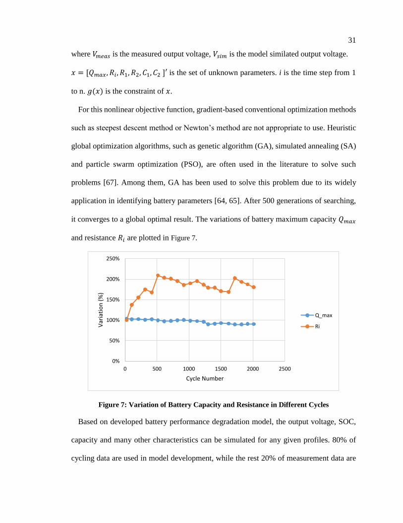
31
where 𝑉𝑚𝑒𝑎𝑠 is the measured output voltage, 𝑉𝑠𝑖𝑚 is the model similated output voltage.
𝑥 = [𝑄𝑚𝑎𝑥, 𝑅𝑖, 𝑅1, 𝑅2, 𝐶1, 𝐶2 ]′ is the set of unknown parameters. i is the time step from 1
to n. 𝑔(𝑥) is the constraint of 𝑥.
For this nonlinear objective function, gradient-based conventional optimization methods
such as steepest descent method or Newton’s method are not appropriate to use. Heuristic
global optimization algorithms, such as genetic algorithm (GA), simulated annealing (SA)
and particle swarm optimization (PSO), are often used in the literature to solve such
problems [67]. Among them, GA has been used to solve this problem due to its widely
application in identifying battery parameters [64, 65]. After 500 generations of searching,
it converges to a global optimal result. The variations of battery maximum capacity 𝑄𝑚𝑎𝑥
and resistance 𝑅𝑖 are plotted in Figure 7.
Figure 7: Variation of Battery Capacity and Resistance in Different Cycles
Based on developed battery performance degradation model, the output voltage, SOC,
capacity and many other characteristics can be simulated for any given profiles. 80% of
cycling data are used in model development, while the rest 20% of measurement data are
0%
50%
100%
150%
200%
250%
0 500 1000 1500 2000 2500
Var
iati
on
(%
)
Cycle Number
Q_max
Ri

32
used to validate the model accuracy. The simulated performance degradation results
showed average 0.88% error. The validation results and errors of battery capacity variation
(𝑄𝑚𝑎𝑥) are plotted in Figure 8.
Figure 8: Validation of Battery Performance Degradation Model
The equivalent circuit built for battery simulation can also be interpreted using
electrochemical impedance spectroscopy (EIS) method (or ac impedance method) [68].
EIS is a powerful tool for the analysis of complex processes of electrochemical reactions.
It has been widely used to capture key characteristics of Li-ion batteries, such as revealing
the influence of operating conditions and SOC on the Li-ion battery impedance [68], or
0 500 1000 1500 2000 2500
Cycle Number
50
60
70
80
90
100
110
Norm
aliz
ed C
apacity
(%) Modeling
Simulation
Validation
500 1000 1500 2000 2500
Cycle Number
0
0.5
1
1.5
2
Err
or(
%)

33
studying the changes of electrode material lattice during the insertion/extraction of
lithium ions [69].
EIS experiments record battery responses by applying a sinusoidal alternating current
(AC) signal with wide spectrums (e.g. from 0.1 mHz to 10 kHz). At above 1000Hz, the
load behaves more like a DC signal for Li-ion battery due to the large time constant of RC
circuit. The battery impedance is the frequency response to the sinusoidal current.
𝑉𝑡(𝑗𝑤) = 𝑍(𝑗𝑤)𝐼(𝑗𝑤) (10)
where 𝐼 is the input current signal, 𝑍 is the impedance, 𝑉𝑡 is the measured voltage.
In order to get the transfer function, the Laplace transformation is applied to the former
developed electrical equivalent circuit model:
𝑆𝑂𝐶(𝑠) = −1
𝑄𝑠𝐼(𝑠)
𝑉𝑖(𝑠) = 𝑅𝑖𝐼(𝑠)
𝑉1(𝑠) =𝑅1
𝑅1𝐶1𝑠 + 1𝐼(𝑠)
𝑉2(𝑠) =𝑅2
𝑅2𝐶2𝑠 + 1𝐼(𝑠)
(11)
The linearized open circuit voltage 𝑉𝑜𝑐 can be showed as:
𝑉𝑜𝑐(𝑠) = 𝛼𝑆𝑂𝐶(𝑠) (12)
where 𝛼 is the coefficient.
The expression of output voltage 𝑉𝑡 in Eq. (7) is re-formulated as:
𝑉𝑡(𝑠) = −
𝛼
𝑄𝑠𝐼(𝑠) − 𝑅𝑖𝐼(𝑠) −
𝑅1𝑅1𝐶1𝑠 + 1
𝐼(𝑠) −𝑅2
𝑅2𝐶2𝑠 + 1𝐼(𝑠) (13)
Therefore, the transfer function can be obtained by combining Eq.(10) and Eq. (13).
𝑍(𝑗𝜔) = −𝛼
𝑄𝑗𝜔− 𝑅𝑖 −
𝑅1𝑅1𝐶1𝑗𝜔 + 1
−𝑅2
𝑅2𝐶2𝑗𝜔 + 1 (14)

34
Based on the identified parameters in the previous equivalent circuit model, a Nyquist
plot of the fresh battery can be obtained by plotting the real part of 𝑍 on the X axis and the
imaginary part on the Y axis (as showed in Figure 9).
Figure 9: Nyquist Plot for the EIS Model
Due to the lack of EIS measurement data, the accuracy of the EIS model built in this
section has not been validated. If more data is available, this model can be used to reveal
the degradation characteristics of battery.
(2) Electrochemical Model (or “Doyle-Fuller-Newman” model)
Electrochemical models are built based on first principles of electro-chemical reactions
during battery charge/discharge processes [70-72]. The first electrochemical model was
proposed by Doyle, et al. [32] in 1993, known as “Doyle-Fuller-Newman” model in the
literature. It adopts a large set of partial differential equations (PDEs) to capture ions’
diffusion dynamics inside the solid materials and soluble electrolyte. These PDEs are

35
highly nonlinear and difficult to solve. Some hypotheses are made in order to improve
its computational ability [73, 74]. If a uniform current density is assumed along both
negative and positive electrodes, the full-order ‘Doyle-Fuller-Newman’ model can be
simplified to a so-called “Pseudo 2-dimensional model” (or P2D). P2D model calculates
the ions’ concentration variation along 2 dimensions: one is the radius of solid compound
particles and the other is the thickness of battery [16]. If the electrolyte concentration is
assumed uniformly inside battery, it is called the “single particle model” (or SPM). SPM
only captures the ions’ movement in one particle of each compound materials on the anode
and cathode. The order of partial differential equations in the original model can be greatly
reduced and hence calculations are much easier.
A demonstration of ion’s movement inside battery during the discharge process is
showed in Figure 10. The external applied current 𝐼 is transformed into microscopic ions
flow rate 𝑗𝐿𝑖. 𝛿𝑛, 𝛿𝑝, 𝛿𝑠𝑝 are the thickness of negative, positive electrode and separator. 𝑥
indicates the direction of battery thickness. As stated before, that discharging current is
positive and charging current is negative.
Figure 10: Demonstration of Ions’ Movement during Discharge
(i) Modelling the Electrochemical Reaction

36
Based on the assumption of uniform current density along electrodes, the ion flow rate
of Li in the battery 𝑗𝐿𝑖 is determined by the applied current. The relationship between the
macroscopic current 𝐼 and microscopic ion flux density is expressed as:
𝐼
𝐴= ∫ 𝑗𝐿𝑖(𝑥)𝑑𝑥
𝛿𝑛
0
(15)
where 𝑗𝐿𝑖 is the ions flux density; 𝛿𝑛 is the thickness of negative electrode; 𝐴 is the
electrode surface area, 𝐼 is the discharge current.
Moreover, the Butler-Volmer kinetic equation builds the connections between the battery
overpotential and microscopic current density:
𝑗𝐿𝑖 = 𝑎𝑠𝑗0 [exp (𝛼𝑎𝐹
𝑅𝑇𝜂) − exp (−
𝛼𝑐𝐹
𝑅𝑇𝜂)] (16)
where, 𝛼𝑎 , 𝛼𝑐 are the anodic and cathodic charge transfer coefficient; 𝑎𝑠 is the active
surface area per electrode unit volume; 𝑅 is the ideal gas number; 𝐹 is the Faraday’s
number. 𝜂 is the overpotential:
𝜂 = 𝜙𝑠 − 𝜙𝑒 − 𝑈(𝑐𝑠) (17)
where 𝜙𝑠 and 𝜙𝑒 are the solid and electrolyte potential, 𝑈 is the equilibrium open circuit
potential, which is a function of solid phase ion concentration (𝑐𝑠).
𝑗0 is the exchange current density at the equilibrium state,
𝑗0 = 𝑘(𝑐𝑒)𝛼𝑎(𝑐𝑠,𝑚𝑎𝑥 − 𝑐𝑠𝑒)
𝛼𝑎(𝑐𝑠𝑒)𝛼𝑐 (18)
where 𝑘 is the reaction rate, 𝑐𝑒 and 𝑐𝑠𝑒 are the electrolyte concentration and SEI
concentration, respectively.
(ii) Modelling of Solid Phase Diffusions
37
The concentration variation inside solid spherical particles is governed by ions’
diffusion process during the intercalation process. Fick’s law is adopted to calculate
concentration change along the radius of solid particle [63].
𝜕𝑐𝑠𝜕𝑡
= ∇𝑟(𝐷𝑠∇𝑟𝑐𝑠) (19)
where 𝑐𝑠 is the ion concentration in the solid particle; 𝐷𝑠 is the solid phase diffusion
coefficient; 𝑟 is the particle radius, and 𝑡 is the time.
The average concentration 𝑐𝑠𝑎𝑣𝑔
is the mean value of total ions installed in the solid
particle:
𝑐𝑠𝑎𝑣𝑔
=1
𝑉∫ 𝑐𝑠(𝑟, 𝑡)𝑑𝑉𝑉
0
(20)
where 𝑉 is the particle volume.
The SOC indicates the proportion of currently stored ions to the maximum available ions.
𝑆𝑂𝐶 =𝜃𝑛 − 𝜃0%
𝜃100% − 𝜃0% (21)
where 𝜃𝑛 =𝑐𝑠𝑎𝑣𝑔
𝑐𝑠,𝑚𝑎𝑥 is the percentage between the actual and maximum concentration. 𝜃100%
and 𝜃0% are parameters depending on the materials.
(iii) Modelling of Solution Phase Diffusions
The movements of ions in the electrolyte are determined by the total current density and
the diffusion rate in the solution. The variation of electrolyte concentration 𝑐𝑒 can be
expressed as:
𝜕휀𝑒𝑐𝑒𝜕𝑡
= ∇𝑥(𝐷𝑒𝑒𝑓𝑓∇𝑥𝑐𝑒) +
1 − 𝑡0
𝐹𝑗𝐿𝑖 (22)

38
where 𝑥 is the direction along battery thickness from anode to cathode; 𝐷𝑒𝑒𝑓𝑓
is the
effective electrolyte phase diffusion coefficient; 휀𝑒 is the electrolyte phase volume fraction;
𝑡0 is the transference number.
Based on the uniform electrolyte concentration assumption, 𝑐𝑒(𝑥, 𝑡) = 𝑐𝑒(𝑡) , the
solution phase concentration variation is simplified as:
𝜕휀𝑒𝑐𝑒𝜕𝑡
=1 − 𝑡0
𝐹𝑗𝐿𝑖 (23)
(iv) The Overall Output Voltage Calculation
The output voltage of Li-ion battery is the overall electrode potential differences minus
the inner resistance voltage drops.
𝑉𝑡 = 𝜙𝑠,𝑝 − 𝜙𝑠,𝑛 − 𝑅𝑓𝐼 (24)
where 𝑅𝑓 is the film resistance inside the cell; 𝜙𝑠,𝑝, 𝜙𝑠,n are the solid phase potential at the
positive electrode (cathode) and the negative electrode (anode).
Numerical solutions are usually adopted to solve these high nonlinear, complex PDEs in
the electrochemical model [71, 73]. This research takes the finite difference method (FDM).
The discretization process of SPM has been put in Appendix A. In total, there are 20
physical and chemical parameters that need to be fit to run this model, which are also
showed in Appendix A. Similarly, GA was adopted to identify these parameters. The
RSME of output voltage calculated from SPM is 8.83%, about ten times higher than the
equivalent circuit model (as showed in Figure 11).

39
Figure 11: Errors of Different Modelling Methods
2.2.3 Battery Life Prediction Model – Equivalent Circuit Model with Degradation
Amendment Term
The battery life prediction model is very important in the hybrid powertrain system
design to support the estimation the total investment cost of battery ESS. More importantly,
it can support the optimal hybrid energy management and achieve a longer battery lifetime,
while maintaining the low operational cost. To fulfill these purposes, the battery
performance and life prediction model is developed in this section. As showed in Figure
12, the battery performance degradation model evaluates the capacity deterioration in each
cycle, and the accumulated performance decay will be used for more accurate lifetime
estimation. As discussed in the previous section, the equivalent circuit model can provide
more accurate result and is easier to implement in the control algorithm. Therefore, the life
prediction model will be incorporated into the equivalent circuit model as the degradation
amendment term.
0
2
4
6
8
10
12
14
16
0 500 1000 1500 2000 2500
Erro
r (%
)
Cycle Number
Equivalent Circuit Model
SPM

40
Figure 12: Battery Performance Degradation and Life Prediction Model
An accurate battery life prediction model should consider all the influence from different
factors: temperature, DOD, and C-rate. It is, therefore, must rely on adequate testing data.
Most researches focus on modelling the battery capacity fading at different operation
temperature [61] [75], or different SOC[76], or the combined temperature and SOC thereof
[77]. The rain-flow cycle counting model [78] and machine learning approaches [66]are
also investigated in battery life prediction models to explore the extreme non-linear aging
process under different usage conditions with moderate cycling experiment data.
Most battery life prediction model developed in the literature [29, 79, 80], combining
both dynamic C-rate and DOD effects, are all built empirically based on pre-acquired
experimental data. However, it usually takes years of time to complete total required tests.
Due to the lack of adequate data in this research, a semi-empirical battery life model is
developed based on the previous work done by many research groups, such as Tsinghua

41
University and The University of Michigan [80], HRL Laboratories and GM Corp. [79],
etc.
This study creatively combines battery SOC (in each mission cycle) and SOH (over
battery lifespan) to accurately estimate battery performance degradation rate and remaining
cycling numbers. The calendar life of battery has minor influence on performance
degradation compared to cycling life [56, 81], therefore, is not considered in our model. It
has been assumed that temperature can be controlled in appropriate ranges by advanced
thermal management system.
The battery capacity losses ( 𝑄𝑙𝑜𝑠𝑠 ) follows Arrhenius kinetics as a function of
temperature, DOD, C-rate and operation time [79]:
𝑄𝑙𝑜𝑠𝑠 = 𝐴 ∙ 𝑒(
−𝐸𝑎+𝐵∙𝐶𝑟𝑎𝑡𝑒𝑅𝑇
)(𝐴ℎ)𝑧
(25)
where, 𝐴 is the pre-exponential factor, 𝐸𝑎 is the activation energy, 𝐵 is the coefficient of
C-rate; 𝑅 is the ideal gas constant, 𝑇 is the temperature, 𝑧 is the exponent of time and
usually is 0.5. 𝐴ℎ is the total throughput capacity as a function of maximum available
capacity (𝑄𝑚𝑎𝑥), cycling numbers (N) and 𝐷𝑂𝐷.
𝐴ℎ = 𝑁 ∙ 𝐷𝑂𝐷 ∙ 𝑄𝑚𝑎𝑥 (26)
After combing Eq. (25) and (26) , battery cycle numbers can be derived as:
𝑁 = (𝑄𝑙𝑜𝑠𝑠
𝐴 ∙ 𝑒(−𝐸𝑎+𝐵∙𝐶𝑟𝑎𝑡𝑒
𝑅𝑇))
1𝑧 1
𝑄𝑚𝑎𝑥 ∙ 𝐷𝑂𝐷
(27)
The unknown parameters in Eq.(27) are 𝐴, 𝐵, 𝑧, and 𝐸𝑎. They have been identified in
the aforementioned literature, and also validated in this study through the LiFePO4 cycle-
life experiment data. The battery life prediction model was implemented in

42
MATLAB/Simulink. The final results of total cycle numbers for this type of LiFePO4 as
a function of 𝐶𝑟𝑎𝑡𝑒 and 𝐷𝑂𝐷 have been plotted in Figure 13.
Figure 13: Battery Cycling Number Prediction under Different C-rate and DOD
The developed battery performance degradation and life prediction model builds a solid
foundation for the hybrid electric marine propulsion design. It brings possibilities for
optimal energy management to prolong battery lifetime through adjusting the battery
discharge C-rate and working DOD.
2.2.4 Summary on Model Fitting and Validation
During this research, 2,000 sets of performance degradation data of a commercialized
lithium iron phosphate (LiFePO4 or LFP) batteries have been acquired from the State-
assigned Laboratory for Electric Vehicle Power Battery Testing in Beijing, China. Large
portions of these data (about 80% of capacity test data) have been used in this work to form
the three types of battery performance degradation models, and the rest 20% data have been
used to validate the accuracy of the models.

43
As discussed in the previous subsections, the first battery performance degradation
model of using equivalent circuit model has 6 model parameters, the model fitting using
least-square fitting method produced a model with relatively accurate simulation result
with RSME of 0.88% after validation. The second battery performance degradation model
used EIS method. Although it lacks EIS data to validate this model, it presented a potential
way in explaining battery degradation mechanisms when the data is available. The third
battery performance degradation model of SPM has 20 model parameters, the model fitting
using least-square fitting method produced a model with relatively higher accuracy of
8.83%.
All three models can be used to support the optimal sizing of the battery ESS and the
optimal energy management of the hybrid electric propulsion system. The EIS model and
SPM model have offered deep insight into the fundamental battery electrochemical
reactions. However, due to the lack of EIS data and the specific battery material
characteristics, the accuracies cannot be guaranteed. Equivalent circuit model, on the other
hand, is more suitable for realistic application in the hybrid propulsion system design.
The 𝑄𝑚𝑎𝑥 used in the battery performance degradation model means maximum capacity
that a battery can store and release, which is also a key parameter that reveals its
degradation degree during lifetime. In general, when 𝑄𝑚𝑎𝑥 has lost 20%, i.e., the 𝑄𝑙𝑜𝑠𝑠 =
20%, the output voltage, power and total energy from the battery will be decreased to a
certain level that can significantly affect total system performance in the hybrid propulsion
systems. Therefore, the battery will be considered as a dead battery and must be replaced.
The variation of 𝑄𝑚𝑎𝑥 has been identified from previous section using equivalent circuit
model. It was stored as a lookup table in the model that can assist model simulation, and

44
provide more accurate available capacity in different cycling numbers. The reduced
capacity, resulted from previous cycles, will be counted in the degradation amendment
term. The remaining cycles before 𝑄𝑙𝑜𝑠𝑠 reaches 20% therefore can be predicted from the
semi-empirical life prediction model.

45
Chapter 3 Hybrid Marine Propulsion System Design, Modelling
and Life Cycle Cost Calculation
The benefits of using hybrid powertrain configurations for land-based and sea-based
transportation have been deeply discussed in the literatures [18, 82]. One of the unique
features of marine vessels that is different from conventional passenger vehicles is its case-
dependent driving/load cycles, as well as hull drag and propeller thrust. This chapter will
introduce the integrated hybrid electric ship-modelling tool based on modularized key
component models. In the developed modelling tool, different hybrid marine propulsion
configurations will be discussed and modelled. Their life cycle cost (LCC) will be
calculated for the economic and environmental comparison.
3.1. Design of Hybrid Marine Propulsion Systems
The design of hybrid marine propulsion system is subjected to the ship application and
the overall hull, propeller performance. In order to focus our research on the marine
propulsion system design, an integrated hybrid electric ship modelling platform is
developed with separated and modularized component models. This ship modelling tool is
implemented in the MATLAB/Simulink environment. However, in order to perform an
accurate simulation, the performance equations/characteristics/maps/coefficients of each
ship component must be acquired from other resources, by either simulation or experiment.
The input/output interfaces between each modular have been clearly defined, so that
different modelling methods can be testified for each component without interfering in
other sub-systems.
A similar system simulator of a marine vessel and its power plant was developed by
researchers in NTNU [83], which is also capable of simulating the mechanical system with

46
diesel engines, the electrical system with generators, and the plant level controller with
dynamic positioning, thrust control and power management system. The marine systems
simulator (MSS) has been developed by Fossen and Perez [84] as a MATLAB/Simulink
library for parametric identification of radiation-force models and fluid memory effects of
marine crafts. Moreover, Fossen also generated a 6 degree of freedom (DOF) unified
dynamic positioning and maneuvering model [85] to simulate ship hydrodynamic forces
and moments. A mathematical model of diesel-electric propulsion systems for marine
vessels has been studied [86], with special attentions on the interconnection of several
synchronous generators to match the power generating part and power consumption part.
These modelling tools focus on ship hydrodynamic calculation and synchronizing the
distribution power grid in hybrid propulsion systems. This dissertation, on the other hand,
will focus on system level hybrid power plant design and energy management for various
marine applications.
3.1.1 The Integrated Hybrid Electric Ship Modelling Tool
This research adopts a modularized modelling method to reduce the complexity of ship
simulation and provide more versatile solutions for ship propulsions. The main ship
components are categorized into several functional modules, while each module can be
built and validated separately before integrated together. The intention of using
modularized modelling method for ship simulation in MATLAB/Simulink environment is
to partition a complicated ship model into several sub-systems. By categorizing all the
components into different modules, it would be much easier to integrate all together
systematically after building and verifying simulation models for each module. The

47
complicity and computational time can also be reduced through defining the input and
output signals between each module instead of tangling all the components together.
As complicated as a bulk ship can be, the ship simulation model can be separated into
four main modules: (1) ship control module; (2) integrated powertrain module; (3)
propeller module; (4) ship maneuvering module. An example of developed simulation
platform for a ferry ship has been showed in Figure 14. The input/output interfaces of these
modules have been clearly defined and presented in Table 4.
Figure 14: Modularized Hybrid Electric Ship Simulation Platform
The integrated powertrain module is the power supply system that consists of all the
prime movers aboard. Depending on the configuration, it could be pure mechanical, pure
electric, or hybrid propulsions. Detailed powertrain design and modelling will be discussed
in the following section. Inside this module, a supervisory controller exists to generate a
high-level control strategy for power distributions between engines and battery ESS.
Intelligent energy management can be developed for this controller.

48
Table 4: Input/output Signals in the Integrated Ship Modelling Platform
Module Input Signal(s) Output Signal(s)
1 Ship Control Module 1.Measured ship course data;
2.Simulated ship velocity (m/s)
1. Power requirement
(kW)
2 Integrated Powertrain
Module 1. Power requirement (kW) 1. Propeller speed (rpm)
3 Propeller Module
1. Propeller speed (rpm)
2. Propeller inflow velocity (m/s)
3. Azimuth angle (if needed)
1. Force (N)
2. Torque requirement
(Nm)
4 Ship Maneuvering
Module
1. Propeller force (N)
2. Wind, wave, current signal
1. Ship velocity (m/s)
2. Propeller inflow
velocity (m/s)
The propeller module takes signals from the powertrain and ship hull-maneuvering
model to determine working conditions for each propeller. The characteristics of propeller
can be stored in pre-generated look-up tables, containing the propeller thrust and torque
coefficient acquired from the full-scaled computational fluid dynamics (CFD) calculation.
The control of propeller can be developed to reduce ship noise and cavitation issues.
The ship maneuvering module accepts thrust forces from propellers and resistances
caused by ship maneuvering and ocean conditions (such as wave, wind, and current) to
calculate the ship hydrodynamic performance. The ship hull resistance and propeller
performance can be modelled through full-scaled CFD simulations, experimental sea trial
and tow tank data, reduced-order or dedicated low-order hydrodynamic model, or generic
mathematical model[87]. The sea experiment and full-scale CFD simulation can provide
more accurate results, however also require expensive time. The dedicated low-order
hydrodynamic model is built through stability book of specific ship hull, or simplified CFD
simulation. The generic parametric mathematical model (GPMM) was developed and
validated by Truelove [87] in the UVic clean transportation team. It can generate

49
representative propeller and steering gear states (torque, speed, power) for any arbitrary
monohull surface vessels, which is very suitable for the ship design and analysis if lacking
of sufficient experimental data.
Ship control model or guidance system compares the simulated ship speed with
measured speed to give instructions to the integrated powertrain module. Both backward-
facing and forward-facing modelling method can be used to develop the integrated
modelling tool. Backward-facing modelling assumes the required power (or torque, speed)
can be satisfied by the power plant at any situation, therefore, the consistency of simulation
results regarding to the desired ones is guaranteed. It is a quasi-steady model thus not
suitable for on-line simulation. Forward-facing control, on the other hand, builds a
driver/captain model to reflect a real-world driving test. It can be implemented in the
hardware-in-the-loop (HIL) system to validate control logics and to get insight into the
limits and design margins of powertrain components.
After finishing the modular simulation and validation, the integrated hybrid electric
modelling tool can be achieved by connecting all the modules together. The systematic
simulation error can be reduced since all the sub-systems have been tested to be accurate
and robust for simulation. Depending on the modelling complexity and accuracy, each
module can have several different approaches, such as power loss model or detailed plant
model. Lookup tables are needed for power loss model. Different ship propulsion
architectures can be built in the powertrain module for the ship design. Detailed
information can be found in Figure 15.

50
Figure 15: Integrated Hybrid Electric Ship Model
Through the modularized ship modelling platform, this research will focus on the
designing, modelling and optimization of hybrid marine propulsion systems in the
integrated powertrain modular.
3.1.2 Design of Hybrid Electric Propulsions
The concept of using electric ship propulsions has been proposed more than100 years
ago [19, 22, 88]. However, there are still not clear definitions on different types of hybrid
electric marine propulsion configurations, regarding the type of energy sources, the path of
power transmission, etc. This section will present a review of conventional marine
propulsions, and propose different hybrid propulsion architectures based on some concepts
from the hybrid electric vehicles.
Hybrid powertrain systems, as discussed in the first chapter, consist two different power
sources: the engine and the Li-ion battery ESS. In automotive industry, the hybrid
powertrain architecture is defined by the way that power is transferred in the driveline. In
general, there are three types of hybrid configurations [89]. The series hybrid powertrain
transforms all mechanical energy from the engine into electrical energy and provides pure

51
electrical drive. The parallel configuration has two energy flow paths, the mechanical
driving from the engine to the wheels via gear sets, or electrical driving from the battery
ESS via electric motor(s). The power split or series/parallel configuration offers more
flexible operation by adopting power split devices (usually a planetary gear set), so that the
energy flow in the drivetrain can be merged electrically and/or mechanically. The power
split hybrid mode combines both advantages from the series and parallel configuration.
Conventional Marine Propulsions
Currently, the majority of ship propulsions are mechanical. The rotational power from
engines (or gas-turbines) is transferred to the propeller through shafts, gearboxes, and
associated couplings[90]. Pure mechanical propulsion is the most convenient structure in
modern ships. One or a few separate engine-generator set(s) (or Genset) must be installed
to provide auxiliary electrical power. A demonstration of mechanical propulsion with two
mine engines (ME) and two Gensets are showed in Figure 16. The blue line indicates
mechanical drive. The red arrowed line shows the electricity flow direction. Main engines
are connected to propellers through clutches and gear reductions.
Figure 16: Mechanical Propulsion Configuration

52
The power take-in (PTI) /power take-off (PTO) configuration are invented to better
facilitate the cooperation between main engines and Gensets [91]. A powerful electrical
motor/generator (MG) is needed. In PTI mode, energy from Gensets can be taken to
support main engines through electrical motors. In PTO mode, extra energy from main
engines will be taken-off to support the auxiliary load through electrical generator. It can
improve the efficiency of main engine and reduce the cost. As showed in Figure 17, the
red line with arrows indicates the electrical energy flow direction. PTO and PIT mode rely
on properly designed power coupling devices, as well as the added electrical machines
(generator/motor).
Figure 17: PTI/PTO Configuration
The electrical propulsion of ships are getting more popular for those exposed to large
power demand variations, such as offshore supply vessels, cruise ships, icebreakers, war
ships, etc. With the rapid development of power electronics and MGs, fully electrified
vessels or so-called all-electric ships (AES) [14] are becoming available in the marine
industry. Through using the integrated power systems (IPS), a common electrical platform
can be built for ship propulsions and service loads through AC or DC power buses [88],
which enables more flexible operations and higher system redundancy and reliability [92].

53
The engines can be cooperated together to fulfill load demand and work in the optimum
energy efficiency point in the meantime.
The attraction of using DC distribution architectures onboard has overwhelmed
traditional AC system, especially in the ships that have heavy electrical loads, such as navy
vessels. The DC system uses power electronic converters to connect all power sources and
load subsystems to a centralized DC distribution bus (Figure 18). The propulsion unit in
the AES can be shaft propeller, azimuth thruster or podded propulsion unit [93]. The shaft
propeller is normally driven by a variable-speed electric motor through a gear reduction.
Azimuth thruster can rotate and produce thrust in any direction, with a vertically mounted
motor and L-shaped gear transmission. The podded propulsion unit also can rotate and
produce trust just like azimuth thruster, but with a compact design that integrated the
electrical motor directly to the propeller shaft inside a sealed pod unit under the vessel hull.
A demonstration of IPS with DC power bus is showed in Figure 18.
Figure 18: Diesel-electric Propulsion with DC Bus

54
Hybrid Marine Propulsions
The hybrid electric propulsion system differs from conventional systems by adding a
large battery ESS to allow the supply of propulsion power from at least two paths. The
ESS disengages the engine speed and the propeller speed, so that the engine can operate at
its most efficient area and the ESS can provide and store energy to support the whole
propulsion system. The main advantages of using hybrid marine propulsions include:
providing more flexible operation;
increasing system redundancy;
improving engine operational efficiency;
reducing fuel consumption and emissions;
reducing engine operational time and maintenance cost;
abolishing the usage of auxiliary Gensets;
The hybrid propulsion systems offer high operating flexibility as well as more
environmental friendly solution. With the fast-developed power electronics and
mechanical transmissions, different hybrid modes can be achieved. Similarly, to the hybrid
automotive configurations, three different hybrid marine propulsions are proposed here for
different using scenarios: series, parallel and series-parallel hybrid systems.
The series hybrid marine propulsion is formed by adding a battery ESS to the integrated
diesel-electrical propulsion. It works as a fully electrified system since all the power from
engines will be transformed into electric energy (Figure 19). The rechargeable ESS acts as
a buffer to store and supply energy. Through optimized powertrain system control, it can
be expected to have lower fuel consumption and emissions compared to the conventional
counterpart. The main advantage of series hybrid mode is that the engine can work in its

55
most efficient area by de-coupling the mechanical connection between the engine and
propeller. If the ESS is sufficiently large, it can provide all required energy and work as
pure electric propulsion.
Figure 19: Series Hybrid Electric Propulsion
Parallel hybrid marine propulsion is very similar to the conventional PTI/PTO
configuration, except to the added battery ESS. Auxiliary Gensets can be retained or
removed, depending on the specific application. Battery ESS can support the requested
electrical energy for auxiliary loads and propulsion loads (Figure 20). The engine and
electrical drives are coupled in a gearbox to propel the thruster. Parallel configuration can
take advantage of mechanical drive from the engine to the propeller directly without
sacrificing energy conversions. Thus, a higher system energy efficiency can be achieved at
the high load demand.

56
Figure 20: Parallel Hybrid Marine Propulsion
The series-parallel hybrid architecture has the most complicated structure and requires
advanced gear sets to transmit the power both mechanically and/or electrically. Planetary
gear sets are largely used in ground hybrid vehicles to work as the electric continuously
variable transmissions (e-CVT) [94]. The limitations and possibilities of applying e-CVT
in power-split marine propulsions are also studied [95], however, it is not a common feature
for marine vessel applications. In this research, a series-parallel hybrid configuration is
realized through four clutches (C1, C2, C3 and C4) and several gear reduction devices, as
showed in Figure 21. The two electrical motor/generators (MG1 and MG2) can work as
generator when charging the ESS, or as motor when using electrical energy to boost the
engines.

57
Figure 21: Series-parallel Hybrid Marine Propulsion
The combination of using both series and parallel hybrid mode provides more flexible
operations and can help achieve higher system efficiency. Although the complexity of
system design is increased, it offers more degree of freedoms to optimize the control
algorithm for a better system performance. Specifically, it can work as in five different
modes:
(1) the pure electric (or series) mode can work under the low or medium power
demands to reduce pollutions, where the power is supplied by the ESS and all
engines are shut down (or operated in high efficiency area to charge the battery);
(2) the engine start mode uses the electrical energy from battery ESS to start main
engines, so that no auxiliary Gensets are needed;
(3) the pure engine mode is more suitable under the high load demand situation, where
the main engines can drive propellers through gear reductions directly with the lest
energy conversion losses;

58
(4) the parallel model allows the ESS and engine work together to create higher
torque/power for the propeller;
(5) the series-parallel mode can be achieved if one of the main engines is operated to
mechanically propel one propeller and electrically drive the motors for another
propeller.
The different operation modes are demonstrated in Table 5. By using two electrical M/G
machines, engines can provide mechanical energy to propeller or split a port of extra energy
to charge the battery. Both MGs can absorb energy from the battery to drive propeller. The
mechanical propulsion path is indicated as green lines and electric propulsion path is
indicated as red lines in different operation modes.
The complexity consideration of implementing series-parallel configuration in marine
vessels is different from automotive industry. Hybrid electric vehicles have different
choices to achieve series-parallel hybrid transformation, either by using planetary gear sets
or a few gear reductions with clutches. A typical example would be the Hybrid Synergy
Drive (HSD), which is a refinement term of Toyota Hybrid System (THS), used in the
Toyota hybrid electric vehicles. The HSD consists of a planetary gear set to provide
continuously variable transmission, therefore, it is also called power-split hybrid
configuration. Although the study of using power-split propulsion system in ships showed
promising feasibility [95], the gear reductions with clutches to change power transmission
paths are more applicable regarding to the cost, reliability, complexity, etc.

59
Table 5: Series-Parallel Hybrid Operation Modes
1. Pure Electric Mode 2.Engine Start Mode
3. Pure Mechanic Mode 4. Parallel Mode
5. Series-Parallel Mode States of Main Components
0: turn off the devices
1: turn on the devices

60
Pure Electric Propulsion
Pure electric propulsion, in this paper, means that the main power sources are purely
electrical components and no engines are adopted. The power sources can be battery,
ultracapacitor, fuel cell, or any of these combinations. It provides only electrical energy to
the motors to drive the propellers. A demonstration of pure electric propulsion with battery
powered ESS is showed in Figure 22.
Figure 22: Pure Electric Marine Propulsion
One thing that must be clarified is that pure electric propulsions require additional
facilities to charge the battery ESS through plugging into the power grid. Similarly, other
hybrid propulsion systems (HES) also can be designed as plug-in hybrid system (PHES) if
charging facility exists.
3.2. Modelling of Hybrid Electric Marine Propulsions
The modelling of hybrid marine propulsion systems is important to facilitate a better
system design. It involves two key aspects: building an accurate detailed model for key
components and developing optimal control strategies for the hybrid energy management.

61
3.2.1. Modelling of Key Components
Key components in former developed hybrid propulsion systems are obviously the
engine and Li-ion battery ESS. The battery performance degradation analysis and
modelling methods are deeply investigated in Chapter 2. Therefore, this section will focus
on the modelling of engine performance and emissions. Other components such as
electrical generator/motors and power electronics are developed using power loss models
with specific efficiency maps.
Both diesel engines and NG-fueled engines are investigated in this research. The fuel
consumption and emissions from marine engines are calculated based on the engine
efficiency and emission maps. The specific fuel consumption maps of different engines are
plotted in Figure 23.
Figure 23: Specific Fuel Consumption Map for Different Engines
The mass of engine fuel consumption (𝑚𝑓𝑢𝑒𝑙) is calculated using the engine specific fuel
consumption map.
𝑚𝑓𝑢𝑒𝑙 = ∫ (𝑃𝑒𝑛𝑔,𝑡 × 𝐵𝑆𝐹𝐶𝑃)𝑑𝑡
𝑡𝑓
𝑡0
(28)
0
50
100
150
200
250
300
350
400
0% 20% 40% 60% 80% 100% 120%fuel
co
nsu
mp
tio
n (
g/kW
h)
% of MCR
Specific Fuel Consumption (g/kWh)
AuxiliaryGenset
LNG Engine
Diesel Engine

62
where 𝑡 is the time step from 𝑡0 to 𝑡𝑓 ; 𝑃𝑒𝑛𝑔,𝑡 (kW) is the power output at time t;
𝐵𝑆𝐹𝐶𝑃(g/kWh) is the brake specific fuel consumption at corresponded power 𝑃.
Various substances and air pollutants are generated during the engine operation. These
emissions are categorized as GHG emissions and criteria air pollutants (CAPs), where each
of them is calculated separately. GHGs normally refer to gases that can trap heat in the
atmosphere and aggravate global warming. According to U.S. Environmental Protection
Agency (EPA), CO2, N2O, and CH4 are the main GHGs emitted from transportation area
[8]. CAPs include a set of common air pollutants that can seriously harm human health and
damage environment [96], such as NOx, SOx, volatile organic compound (VOC), PM,
carbon monoxide (CO), ammonia (NH3), etc. NOx and SOx can cause smog and contribute
to respiratory problems. PM that are 10 micrometers in diameter or smaller can enter into
human bodies, affecting heart and lungs.
In this study, GHG, include CO2, N2O, and CH4 are calculated. CAPs, include SOx, NOx
and PM, are calculated. For each mission call, engine emissions (𝐸) are determined by the
corresponded emission factors [97].
𝐸 = ∫ (𝑃𝑒𝑛𝑔,𝑡 × 𝐸𝐹𝑃)𝑑𝑡
𝑡𝑓
𝑡0
(29)
where 𝐸𝐹𝑃(g/kWh) is the emission factor at power P.
Among all the exhausted emissions, CO2 and SO2 are mainly determined by the content
level of carbon and sulphur in different fuel type. The 2018 Canada’s National Greenhouse
Gas Inventory Report compares GHG emissions from various types of fossil fuel [98]. In
which, it presented specific emission factors of CO2, CH4 and N2O from refined petroleum
products and natural gas. More specifically, it listed emission factors from marine fuels
(showed in Table 6).

63
Table 6: Emission Factor of Different Marine Fuels [98]
Emission Factors from Marine Fuel (g/L fuel)
CO2 CH4 N2O
MGO 2307 0.22 0.063
MDO 2681 0.25 0.072
HFO 3156 0.29 0.082
Natural Gas (Marketable1) 1.926 0.000037 0.000033
Considering the CH4 leakage for LNG-fueled marine engines, the CH4 emission factor
is adjusted according to the study from Bengtsson, et al. [23]. They have showed a more
reasonable CH4 emission factor from Wärtsilä LNG dual-fuel engines (including CH4 slip)
at 0.3g/MJ.
To compare the reduced emission by using electricity from the power grid in hybrid
propulsions, emission factors of BC Hydro’s electricity are also acquired. Since BC has
92% electricity from hydro power, the carbon emissions is about 11tonne per GigaWh [99].
The emission of CH4 and N2O can be neglected in the electricity production.
In conclusion, the GHG emission factors from using diesel, LNG, and electricity in BC,
Canada are listed in Table 7.
Table 7: GHG Emission Factor from Different Energy Sources
GHG Emission Factors [98]
CO2
(kg/kg fuel)
CH4
(kg/kg fuel)
N2O
(kg/kg fuel)
Diesel 3.060502 0.285388 0.082192
LNG 2.4075 0.0135 [23] 0.00004125
CO2
(g/kWh)
CH4
(g/kWh)
N2O
(g/kWh)
Electricity 11 --- ---
1 The term “marketable” means it only applies to fuel consumed by the Electric Utilities, Manufacturing Industries, Residential/Commercial and Transport subsectors, which does not include the raw gas consumption. [98]

64
The concept of total equivalent CO2 (CO2e) is adopted to weight the global warming
impacts of different types of GHG with respect to the effects of CO2. The 100-year Global
Warming Potential (GWP) is acquired from the website of U.S. Environmental Protection
Agency (EPA). Specifically, the GWP for CH4 and N2O are 25 and 298, respectively. CO2e
can be calculated by multiplying GWP values to each GHG.
The SOx emission is a function of sulfur content in the fuel. If assuming all the sulphur
content in the fuel are converted to SO2, a mass-balanced approach can be used to calculate
SOx emission factor [100].
𝐸𝐹𝑆𝑂𝑥 = 𝑆% ×
𝑚𝑜𝑙𝑒𝑐𝑢𝑙𝑎𝑟 𝑚𝑎𝑠𝑠 𝑜𝑓 𝑆𝑂2𝑎𝑡𝑜𝑚𝑖𝑐 𝑚𝑎𝑠𝑠 𝑜𝑓 𝑆
× 𝐵𝑆𝐹𝐶 (30)
where, 𝐸𝐹𝑆𝑂𝑥 is the emission factor for SOx (g/kWh); 𝑆% is the sulphur content of the
marine fuel; 𝐵𝑆𝐹𝐶 is the Brake Specific Fuel Consumption of the engine (g/kWh).
Specifically, sulphur content 𝑆% = 0 for LNG engine (assume all sulphur were
removed from natural gas during the liquefaction process). 𝑆% = 0.000015 for ULSD
diesel fuel.
NOx is a harmful emission from marine industry that can form smog and contribute to
respiratory problems. It is caused by the nitrogen present in the atmosphere reacted with
oxygen under the high temperatures and pressures in combustion engines. Many studies
show relatively high emission factor for NOx due to the outdated engine technology [97,
101]. A new designed medium speed diesel engine must meet about 2g/kWh NOx emission
standard to comply with the tier III NOx emission standards in the ECAs. The LNG dual-
fuel engine from Wärtsilä shows that NOx emission factor is 1.3 g/kWh., according to [23].

65
PM is a result of incomplete fuel combustion, including carbon particles, sulphates
and nitrate aerosols. Fuels with higher sulphur content usually generate more PM. PM
emission factors from LNG and ULSD are 0.04 and 0.25 g/kWh, respectively [102].
The efficiencies of other electrical components and power converters in the hybrid
marine propulsion systems are showed in Table 8. These values are based on the averaged
efficiencies of different power electronics and electrical machines [35, 103, 104].
Table 8: Efficiency of Electrical Components
Component Efficiency
Generator and Controller 0.94
Battery ESS and Battery Control Unit 0.99
Motor and Motor Controller 0.94
Battery Charging Facility 0.93
The battery charging facility efficiency highly depends on the charging power. The
number we used here is according to the charging efficiency data acquired from charging
Tesla electric vehicles.
3.2.2. Hybrid Energy Management (Control Algorithm Development)
Control algorithms in the hybrid energy management system (EMS) can make a huge
impact on the overall system performance. The existing of battery ESS enables more
flexible operation, also increases the complexity of control hierarchy. EMS takes different
control laws to decide the power distribution among different energy sources under certain
load profiles. The hybrid EMS usually consists some parallel lower level controllers for
each component, such as the engine control unit (ECU), battery management system
(BMS), and motor control unit (MCU). Above them, a supervisory controller is built in
higher level. The supervisory controller can collect information, make decisions and give
instructions to the specific lower level controller (as shown in Figure 24). In general, the

66
energy management problem is to find the optimal control law for a given system under
defined load profile over a finite time horizon. The objective of the energy management
control in hybrid powertrain systems is to achieve the minimum fuel consumption, reduce
emissions and prolong battery lifetime [89].
EMS
Supervisory controller
ECUBMS MCU …...
Battery ESS
battery control
Engine
engine control
Motor
motor control
Figure 24: Control Topology in Hybrid Marine Propulsion Systems
The general methods that used in hybrid energy management system can be separated
into two categories: the rule-based and model-based optimization methods [89]. Rule-
based control logic is a heuristic approach and very effective in real-time implementation.
Rules normally acquired based on intuition, experiences, or results from other global
optimization methods, therefore, they are not guaranteed to be optimal control rules. Due
to its simplicity and easy implementations, it has been widely applied in the optimal design
of electric vehicle [36].
Model-based optimization strategies can find a global optimal solution for the system by
minimizing a cost function over a fixed load profile. To this end, the model-based
optimization control logic must have a known load profile in advance and perform
intensive computation to acquire the optimal solution. Both online and offline optimal

67
control strategies have been investigated in the literature [20]. The optimization methods
can be numerical or analytical, depending on the formulated problem. The most important
thing in model-based optimizations is to find the optimal control laws through optimal
control theory.
Optimal control theory deals with the problem of finding a control law for a dynamic
system such that a certain optimality criterion is achieved. A control problem includes a
cost function that is a function of state and control variables. Early work of optimal control
dates back to 1950s with the fundamental researches done by Richard Bellman (1920-
1984) and Lev Pontryagin (1908-1988) [105]. Dynamic programming (DP), introduced by
Bellman, is still the state-of-the-art method used to solve optimal control problems [37].
The development of minimum principle by Pontryagin (also known as Pontryagin
Minimum Principle, or PMP) provides necessary conditions to find the optimal controls
[106]. Later in 1980s, reinforcement learning (RL) was developed to deal with more
complex control problems that have difficulties to obtain system model. Intelligent control
algorithms such as neural networks (NNs) [107], model predictive control (PMC) methods
[108], fuzzy logic control [109], etc. provide new ideas to solve the nonlinear control
problem.
DP and PMP are the most widely applied methods that can find the theoretical optimal
control solution for the hybrid systems in a known load profile. They can only applicable
offline and require a priori knowledge about the entire optimization horizon to give the
optimal trajectory. DP is a numerical algorithm that can be used to solve a continuous
control problem by discretizing the state variables, while PMP can form an analytical
formulation for the problem and find a closed-form solution so that the ideal results can be

68
found. Equivalent Consumption Minimization Strategy (ECMS) defines an
instantaneous cost function at each time step during the total time horizon, which can lead
to the global optimal control strategy if the instantaneous minimization problem is solved
appropriately. ECMS approach uses models to convert electricity consumption to an
equivalent amount of fuel, and then makes real-time power split decisions to minimize the
net fuel consumption. Therefore, ECMS can be used as online optimal control approach.
The comparisons of three typical control strategies are showed in Table 9.
Table 9: Comparison of Different Control Strategies
Rule-based ECMS Dynamic
Programming
Type Heuristic Model-based
optimization
Model-based
optimization
Application on-/off-line online offline
Optimality Not optimal Instantaneous-optimal Horizon-optimal
Driving cycle pre-
request
No Yes Yes
Computational
Intensive
Low Low High
To achieve the real-time optimal control for hybrid electric powertrain systems, the
approximate PMP (A-PMP) [110] or adaptive dynamic programming (ADP) [111]
algorithm is developed. Their aim are to develop the optimal control that is not relying on
the priori knowledge of the future driving conditions, thus, can be implemented in real-
time online system.
3.3. Life Cycle Cost Model of Hybrid Marine Propulsions
The life-cycle cost (LCC) model is built in this section to reflect economic influences of
hybrid marine propulsions to the whole ship life time operation. It includes capital and
operational cost from main powertrain components (i.e. power sources, electric machines

69
and power converters). The costs of other ship elements such as hull and propellers have
been excluded; however, they can be easily added into the results to find the total ownership
costs (TOC). All the cost and/or price in this study are given in Canadian dollars.
Traditional LCC calculation methods in the marine industry, such as the LCC from
NORSOK standards[112], are not suitable for the evaluation of hybrid marine propulsion
systems. Due to the cost-intensive Li-ion battery ESS and its relatively short lifetime, it is
important to evaluate the battery replacement cost and residual cost during the total ship
life.
In this study, a new LCC model for hybrid marine propulsions is proposed. The main
elements in the LCC model include the capital cost (𝐶𝑐𝑎𝑝), operational cost (𝐶𝑜𝑝𝑒), and
residual cost (𝐶𝑟𝑒𝑠𝑑).
𝐿𝐶𝐶 = 𝐶𝑐𝑎𝑝 + 𝐶𝑜𝑝𝑒 + 𝐶𝑟𝑒𝑠𝑑 (31)
The net present value (NPV) analysis is used in the LCC model to calculate the present
value of cash flows over the entire lifetime. After setting the base year cost, the future cost
is discounted back to the base year so that present value of the cost flow can be represented.
𝑁𝑃𝑉 =∑𝐶𝑡
(1 + 𝑟)𝑡
𝑁𝑡
𝑡=0
(32)
where 𝐶𝑡 is the net cost in year t, which can be assumed equally for every year; 𝑁𝑡 is the
total lifetime in year; 𝑟 is the annual discount rate/inflation rate.
3.3.1 Capital Cost
The capital cost (𝐶𝑐𝑎𝑝) includes all the purchase cost for main propulsion components.
The reinvestment cost of Li-ion battery ESS must be considered due to its short lifespan

70
compared to engines and other components. Moreover, for NG-fueled engines and
hybrid propulsions, additional cost may occur.
𝐶𝑐𝑎𝑝 = 𝐶𝑒𝑛𝑔 + 𝐶𝑏𝑢𝑘 + 𝐶ℎ𝑦𝑏 + 𝐶𝑒𝑠𝑠 + 𝐶𝑐ℎ𝑎𝑔 + 𝐶𝑟𝑖𝑛 (33)
where, 𝐶𝑒𝑛𝑔 is the engine cost;
𝐶𝑏𝑢𝑘 is the bunkering system and gas storage cost for NG-fueled engines;
𝐶𝑒𝑠𝑠 is the battery ESS cost;
𝐶ℎ𝑦𝑏 is the cost for hybridization and electrification, including purchasing the electric
motors/generators and power converters;
𝐶𝑐ℎ𝑎𝑔 is the charging facility cost for plug-in hybrid propulsion systems;
𝐶𝑟𝑖𝑛 is the reinvestment cost due to the replacing of battery ESS;
Engine and ESS cost (𝐶𝑒𝑛𝑔 and 𝐶𝑒𝑠𝑠) are related to component sizes and prices.
𝐶𝑒𝑛𝑔 = 𝑝𝑒𝑛𝑔𝑃𝑒𝑛𝑔 (34)
𝐶𝑒𝑠𝑠 = 𝑝𝑒𝑠𝑠𝐸𝑒𝑠𝑠 (35)
where 𝑃𝑒𝑛𝑔 and 𝐸𝑒𝑠𝑠 are the engine power (kW) and battery ESS energy (kWh), and 𝑝𝑒𝑛𝑔
and 𝑝𝑒𝑠𝑠 are the prices for engine ($/kW) and ESS ($/kWh).
𝐶𝑟𝑖𝑛 is the reinvestment cost, counting for the replacement cost of battery ESS due to the
lower lifetime. The operation life of battery ESS (𝐿𝑏𝑎𝑡) is calculated based on developed
battery life prediction model in Chapter 2.
𝐶𝑟𝑖𝑛 =∑𝐶𝑒𝑠𝑠
(1 + 𝑟)𝑡𝑘𝑡
𝑁𝑡
𝑡=0
(36)
where 𝑘𝑡 is the replacement frequency, which is a function of the battery lifetime (𝐿𝑏𝑎𝑡).
𝑟 is the annual inflation rate. 𝐿𝑏𝑎𝑡 is the key parameter that determines the reinvestment

71
capital costs. The optimal result of 𝐿𝑏𝑎𝑡 must be determined at the system level
considering both engine and ESS operation conditions.
𝑘𝑡 = 𝑓(𝐿𝑏𝑎𝑡) = {1, 𝑚 = 𝑛 ∙ 𝐿𝑏𝑎𝑡, 𝑚 ≤ 𝑁𝑡0, 𝑜𝑡ℎ𝑒𝑟𝑤𝑖𝑠𝑒
(37)
where 𝑚 is the year time when replacement occurs in the whole lifespan 𝑁𝑡, i.e., the when
the battery life is ended. 𝑛 is integer numbers, 𝑛 = 1,2,3… When the battery needs to be
replaced in year 𝑚, then 𝑘𝑡=1, otherwise, 𝑘𝑡 is 0.
3.3.2 Operational cost
Operational cost is generated during the lifetime operation, including the energy
consumption and engine maintenance cost. Other costs related to the ship insurance,
registration, etc. are excluded.
𝐶𝑜𝑝𝑒 =∑𝐶𝑒𝑛𝑒𝑟𝑔𝑦 + 𝐶𝑚𝑎𝑖𝑛𝑡
(1 + 𝑟)𝑖
𝑁𝑡
𝑖=0
(38)
where 𝐶𝑒𝑛𝑒𝑟𝑔𝑦 , 𝐶𝑚𝑎𝑖𝑛𝑡 are cost for energy consumption and engine maintenance. 𝑟 is the
annual inflation rate. 𝑖 is the year from 0 to 𝑁𝑡.
Three different types of energy occurred in proposed hybrid propulsion systems: the
LNG, diesel (specifically ULSD), and electricity. The energy cost is dependent on total
energy consumption and the price.
𝐶𝑒𝑛𝑒𝑟𝑔𝑦 = 𝐶𝑓𝑢𝑒𝑙 + 𝐶𝑒𝑙𝑒𝑐 (39)
where 𝐶𝑓𝑢𝑒𝑙, 𝐶𝑒𝑙𝑒𝑐 are costs for marine fuel and electricity respectively.
𝐶𝑓𝑢𝑒𝑙 = 𝑝𝑓𝑢𝑒𝑙 ∙ 𝑚𝑓𝑢𝑒𝑙 (40)
where 𝑝𝑓𝑢𝑒𝑙 is the price of marine fuel ($/kg); 𝑚𝑓𝑢𝑒𝑙 is the total mass of consumed fuel
(kg).

72
𝐶𝑒𝑙𝑒𝑐 = 𝑝𝑒𝑙𝑒𝑐 ∙ 𝑒𝑒𝑙𝑒𝑐 (41)
where 𝑝𝑒𝑙𝑒𝑐 is the price of electricity ($/kWh); 𝑒𝑒𝑙𝑒𝑐 is the total charged electricity from
grid (kWh).
The energy prices are varied with different types of fuel as well as the end-user groups.
And they are the key factors for the total operation cost evaluation. To be clear, prices in
this study are intended for industrial consumers in BC, Canada.
(1) Marine Fuel Price in BC
Canada has a large reservation volume of natural gas and is ranked as the fourth largest
producer of natural gas in the world. The variation of natural gas price can be found from
AECO hub, which is Canada’s largest natural gas trading hub [113]. As the marine fuel,
the LNG price consists of the cost from the natural gas, the liquefaction, the storage and
distribution. Analysis shows that liquefaction cost can be as high as the gas price itself,
which is a significant part of the total LNG cost.
A report from the Canadian Natural Gas Vehicle Alliance [102] has estimated all the
costs for natural gas liquefaction, delivery and storage, based on the existing facilities
utilization in BC. More information have been collected from U.S. Energy Information
Administration (EIA) [114], The Alberta Market Price of natural gas [115], BC Ferries fuel
strategies report [116], Canadian Natural Gas Vehicle Alliance [102], etc. In conclusion,
the price of marine fuels are assumed as $10/GJ for LNG and $24/GJ for ULSD in BC,
Canada.
(2) Electricity Price in B.C.
Electricity price differs across the whole country due to a number of factors, such as the
main type of power generation and the market structure. British Columbia offers one of the

73
lowest electricity prices in Canada. Benefitting from its 92% hydroelectricity, BC hydro
provides low-cost and less GHG emission for all the customers [117].
A report from Hydro Quebec has compared the annual rate of industrial electricity prices
for different jurisdictions in North America [118]. According to a report from the
Association of Major Power Customer of BC (“AMPC”), BC Hydro’s industrial rates have
risen faster than other Canadian jurisdiction since fiscal 2011 [119]. The industrial
electricity price in Vancouver, BC with provincial sales tax (PST) is 5.87¢/kWh in fiscal
2017.
In conclusion, the prices of energy used in proposed propulsion system are presented in
Table 10.
Table 10: Comparison of Energy Prices
Energy Type USLD LNG Electricity
Price (Cad$) 1.04($/kg) 0.45($/kg) 0.0587($/kWh)
Engine maintenance and repair occur periodically during its lifetime. Engines need
regular inspection and maintenance to keep it operating properly. The maintaining cost is
highly relevant to its maintaining schedule, which is a function of total operation time.
Estimating maintenance cost has been difficult as it varies with yearly operational time,
manufacturers, and specific maintaining contents. Since engine maintenance cost is closely
related to its working time and the initial capital cost (largely associated with engine size).
It is assumed that the maintenance will cost half of the engine’s initial purchase cost each
10,000 hours, including all the required lubrication oil change, parts replacement and labor
fee.

74
Maintenance cost for LNG engines are considered lower than diesel engines according
to the engine vendor [25]. Since natural gas fuel is cleaner, equipment tends to have lower
inspection frequency due to reduced deterioration of the fuel supply system. LNG engines
are estimated to have 9% lower maintenance cost over the whole life time compared to
conventional diesel engines [120].
3.3.3 Residual Cost
The residual cost (or salvage cost) of replaced Li-ion batteries is nontrivial for this
expensive component. As stated before, it is usually considered to replace the battery ESS
from hybrid propulsion system in transportation application when the battery capacity
reduces to 80%. Retired batteries from hybrid transportation vehicles can be reused for
residential energy storage and load leveling in the smart grid application. Research has
showed that the second use of a Li-ion battery can be provided at a relatively low price
based on the techno-economic analysis [121].
In this study, residual cost is the remaining value in the replaced battery ESS, which is
also determined by the replacement times and residual price.
𝐶𝑟𝑒𝑠𝑑 =∑𝑝𝑟𝑄𝑟(1 + 𝑟)𝑖
𝑘𝑖
𝑁𝑡
𝑖=0
(42)
where 𝑝𝑟 is the price for the remaining value ($/kWh), 𝑄𝑟 is the remaining capacity (kWh),
and 𝑟 is the annual inflation rate.

75
Chapter 4 Combined System Design and Control Optimization
of Hybrid Electric Marine Propulsions – Application on a
Harbour Tugboat
This chapter aims at finding the optimal hybrid electric marine propulsion system
according to the specific requirement from different vessels. To reach the optimal result,
both the plant design and system control must be addressed jointly in a combined
optimization problem. Global optimization algorithms are reviewed in order to solve this
problem. Surrogate model-based approach is adopted to improve the computational
efficiency and ensure the global optimum.
The application of combined hybrid system design and control optimization in the
marine industry, to the best of the author’s knowledge, has not been studied before.
Therefore, a case study on the optimal design of hybrid electric propulsion system of
harbour tugboats is shown in this chapter.
4.1 Literature and Motivation
Modern challenging hybrid powertrain system design involves two critical aspects,
determining the power specification of main components (sizing) and distributing the
energy requirements among different power sources (controlling). Existing studies of
optimal hybrid powertrain system design mostly focus on the component sizing to reach
the minimum fuel consumption, emission, or their combinations [36, 122]. Control
algorithms for hybrid energy management are usually obtained/optimized based on the
selected (not necessarily optimized) power components [37, 123]. The commonly used
optimal control algorithms in hybrid electric vehicles include DP, PMP and ECMS, which
have been discussed in Chapter 3. These online and offline optimal control algorithms have

76
been widely investigated for HEVs [124] and PHEVs [20]. However, the isolated
optimization processes for powertrain dimensioning and control system development do
not guarantee a global optimal solution for the system design. Recently, more and more
researchers realized the coupled condition of these two design problems and developed
combined design and control optimization framework.
The combined hybrid system optimal component sizing and optimal control are complex
and computationally intensive. Usually, a bi-level optimization framework is adopted to
solve the combined design and control problem [125] [40, 126], in which the inner loop
deals with the optimal control problem and the outer loop using different algorithms to find
the optimized component size. Patil [39] utilized a coupling term to capture the dependence
of the optimal control solution on the battery size to reduce the computational time for the
optimal design and control of a PHEV. A comparison of different bi-level optimization
methods, with the inner loop using the DP and the outer loop using the GA, sequential
quadratic programming (SQP), PSO and pattern search are discussed [126]. However, the
Li-ion battery performance degradation is seldom considered in aforementioned studied
due to the lack of accurate life prediction model. In general, the combined design and
control optimization problem is highly nonlinear, non-convex, and expensive to compute.
There is an urgent need to find an effective method to solve this type of problem.
Metamodelling-based optimization method can effectively reduce computational time
through building explicit approximation (or surrogate model) of the original expensive
simulation model, therefore, it can afford much quicker computation. Some gaps remain in
using surrogate models to solve hybrid powertrain system design, especially in marine
industry. To address this problem, this study initiatively adopts metamodelling approach

77
to solve the complex integrated design and control optimization problem for hybrid
electric marine propulsion system. To conclude, some creative ideas in this chapter include:
adopting a detailed Li-ion battery performance degradation and life prediction
model to support battery lifetime estimation;
using the LCC model as the main objective function of the hybrid marine
propulsion design, which can reflect the influences from both the component
sizing and control algorithm;
formulating the integrated optimal design and control problem in a bi-level,
nested optimization framework;
building a surrogate model to solve the nested optimization problem with
improved computational efficiency;
In the following part of section 4.1, global optimization methods that are commonly used
in solving engineering problems are reviewed. Some background knowledge of solving
nested optimization problem through surrogate modelling method is also introduced. In the
next few sections from 4.2 to 4.4, the proposed approach is applied for the design of
harbour tugboats’ hybrid propulsion system. The optimized design solution, acquired
through nested optimization for combined system design and control, provides the best
result as a benchmark for other design solutions.
4.1.1 Global Optimization Algorithms
Optimization algorithms are essential in finding the best solution of complex real-life
engineering design problems. The general optimization approaches can be separated in to
analytical methods, graphical methods, experimental methods, and numerical methods
[127]. Classic optimization techniques are analytical methods based on the differential

78
calculus which can guarantee to find the global optimal within finite time. Graphical and
experimental techniques are of limited usefulness in practical applications due to the
complicity of objective functions and constraints. Numerical methods are the most widely
applied approaches in solving highly nonlinear complex optimization problems. It is also
referred as mathematical programming in optimization community, in which iterative
numerical evaluations are executed to generate progressively improved solutions.
Commonly used mathematical programming includes linear programming, quadratic
programming, nonlinear programming, dynamic programming, etc. [127].
Gradient-based classic optimization methods (such as Newton algorithm) require
mathematically described objective functions that limit their applications in solving some
engineering problems. Heuristic algorithms, on the contrary, are often gradient-free rules
that can solve problems when classic methods fail to. Heuristics can find a “good enough”
solution in limited time; however, it is hard to measure how close the solution is to the
global optima. The trade-offs between the accuracy and computational time have to be
clearly considered. Meta-heuristics are higher-level heuristic algorithms that can provide
more accurate solutions by generating a set of heuristics iteratively. Most of meta-heuristics
are derivation-free, which means they optimize problem stochastically and iteratively. The
optimization process starts with random initial values and there is no need to calculate the
derivative of search spaces to find the optimum. The stochastic nature of meta-heuristics
allows them to easily avoid local optima and search the entire design space extensively.
They normally use more sophisticated methods to search globally in the feasible domain
and to accept a temporary deterioration of the solution to escape from the local optima.
Most of searching algorithms in meta-heuristics are inspired by nature phenomena. Meta-

79
heuristic methods are very popular in solving complex optimization problems due to the
simplicity, flexibility, derivation-free mechanism, and local optima avoidance [128].
Nature-inspired meta-heuristic algorithms have been developed over past few decades to
solve complex optimization problems with increased problem sizes. Depending on their
inspired nature phenomena, the meta-heuristics can be classified as: (1) evolutionary-based
algorithms, such as genetic algorithm (GA) [129]; (2) physics-based algorithms which
mimic physical rules in universe, such as Gravitational Search Algorithm (GSA) [130]; (3)
population-based, or swarm intelligence-based algorithms, such as Particle Swarm
Optimization (PSO) [131] and Ant Colony Optimization (ACO) [132]. Population-based
meta-heuristic algorithms take advantages from multiple candidate solutions and can better
avoid local optima compared to single-solution-based algorithms. The recent popular
population-based searching algorithms include the grey wolf optimizer (GWO) [128], the
lion optimization algorithm (LOA) [133], and the whale optimization algorithm.
It is usually computationally demanding when apply the meta-heuristics in solving
complex optimization problems. It also has to be clarify that no meta-heuristic optimization
algorithm that is best suitable for solving all optimization problems, as proved by No Free
Lunch (NFL) theorem [134]. In other words, the selections of using which optimization
algorithm in specific complex engineering problem rely heavily on engineering
experiences. The searching process of population-based meta-heuristic algorithms can be
divided into two phases: exploration and exploitation. Exploration determines the way to
search for new peaks in unexplored area, while exploitation makes the best decision at
given current information. A robust optimization algorithm must balance between the

80
exploration and exploitation to achieve the best performance in searching for the global
optimal result.
It is considered as a multi-objective optimization (MOO) problem if a set of different
objective functions are optimized simultaneously [135]. The primary goal of MOO is to
model the preferences of a decision-maker, where the relative importance of objectives has
to be indicated. Different methods can be implemented in solving this type of problems.
Depending on how the preferences are articulated, the solutions can be categorized as priori
articulation, posteriori articulation, or progressive articulation of preferences, where the
decision-maker indicates the relative importance of goals before running the optimization
algorithm, after acquiring a set of potential solutions, or adapting inputs during the running
of algorithm.
4.1.2 Combined Plant and Controller Optimization
The combined plant design and control optimization has been a difficult task for various
applications, mainly due to the increased complexity caused by coupled conditions
between the plant and its controller. It is sometimes referred as the co-design problem.
Reyer [136] and Fathy [38] has deeply discussed various solution strategies for those
combined design and control problems, considering the optimality conditions and whether
those strategies can find the true system optimum. These strategies can be classified as:
sequential strategy: optimizing the plant first and then the control. This is naturally
followed the system design sequence and often leads to a non-optimal solution;
iterative strategy: operating the optimization algorithm iteratively, first optimize the
plant without sacrificing controller performance, then optimize the control algorithm
without compromising plant design;

81
simultaneous strategy: formulating the system optimization problem as a function
of the two sub-systems (including the objectives and constraints), however the
solution can be mathematically and computationally challenging [137];
bi-level, nested strategy: combining separated design and control optimization
problems into two optimization loops in a nested way, the outer (or upper) loop
optimizes the plant design, while the inner (or lower) loop generate the optimal
control algorithm for each plant selected by the outer loop;
partitioned strategy: formulating a master problem to govern the interactions between
the design problem and control problem, which is a common approach for
multidisciplinary optimization problems.
The last three methods is extremely suitable for plant and controller optimization on the
coupled conditions, whereas if they are solved sequentially or iteratively, the results are
not guaranteed to be the optimum for the combined situation [38]. The definition and
quantification of coupling are discussed by Peters [138]. A graphical illustration of
different approaches are presented in Figure 25.
The intricate design and control problem of hybrid powertrain systems can be formulated
as a nested optimization with multi-objectives. Patil [39] in his dissertation, specifically
focused on combined PHEV system design and control optimization to minimize CO2
emissions and costs and maximize its synergistic interaction with the electric grid. It
tackled two optimal control problems for a series PHEV: the on-road power management
and the charging strategy. A review of optimization strategies used in the nested problem
shows that DP is the most widely accepted benchmark in developing optimal control

82
algorithm (in the inner loop), where GA and PSO are the most commonly used
algorithms for component sizing (in the outer loop) [139].
Figure 25: Solutions for Coupled Design and Control Problems (followed [38, 138])
In the bi-level, nested optimization problem, the upper level is usually referred to plant
design and typically expressed as a static optimization problem of the following form [38]:

83
min𝑥𝑝
𝑓𝑝
subject to: ℎ(𝑥𝑝) = 0
𝑔(𝑥𝑝) ≤ 0
(43)
where 𝑥𝑝 is the plant design variable, ℎ and 𝑔 are the upper level equality and inequality
constraints.
The lower level optimization problem is commonly formulated as a dynamic
optimization problem as showed below:
min
𝑢(𝑡),𝑥(𝑡),𝑡0,𝑇{𝛷(𝑥(𝑇), 𝑇) + ∫ 𝐿(𝑥(𝑡), 𝑢(𝑡), 𝑡)𝑑𝑡
𝑇
𝑡0
}
subject to:
𝑥(𝑡)̇ = 𝑓(𝑥(𝑡), 𝑢(𝑡), 𝑡)
𝛹(𝑥(𝑇), 𝑇) = 0
𝜂(𝑢(𝑡), 𝑡) ≤ 0
𝑥(𝑡0) = 𝑥0
(44)
where 𝑢(𝑡) is the control variable, 𝑥(𝑡) is the system state variable, 𝑡0 and 𝑇 are the initial
and end of time, 𝛹 and 𝜂 are the lower level equality and inequality constraints, 𝑥0 is the
initial state value. 𝛷 and 𝐿 are cost functions at the final state and during the controlling in
the driving profile.
The combined plant/controller design must satisfy all the constraints on the individual
problems and also the influence of the plant design on the lower level controller
optimization. The two objectives can be weighted together in the combined nested
optimization problem through 𝑤𝑝 and 𝑤𝑐 . Hence, the combined plant/controller
optimization problem becomes:
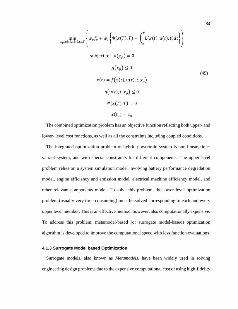
84
min𝑥𝑝,𝑢(𝑡),𝑥(𝑡),𝑡0,𝑇
{𝑤𝑝𝑓𝑝 + 𝑤𝑐 {𝛷(𝑥(𝑇), 𝑇) + ∫ 𝐿(𝑥(𝑡), 𝑢(𝑡), 𝑡)𝑑𝑡𝑇
𝑡0
}}
subject to: ℎ(𝑥𝑝) = 0
𝑔(𝑥𝑝) ≤ 0
𝑥(𝑡)̇ = 𝑓(𝑥(𝑡), 𝑢(𝑡), 𝑡, 𝑥𝑝)
𝜂(𝑢(𝑡), 𝑡, 𝑥𝑝) ≤ 0
𝛹(𝑥(𝑇), 𝑇) = 0
𝑥(𝑡0) = 𝑥0
(45)
The combined optimization problem has an objective function reflecting both upper- and
lower- level cost functions, as well as all the constraints including coupled conditions.
The integrated optimization problem of hybrid powertrain system is non-linear, time-
variant system, and with special constraints for different components. The upper level
problem relies on a system simulation model involving battery performance degradation
model, engine efficiency and emission model, electrical machine efficiency model, and
other relevant components model. To solve this problem, the lower level optimization
problem (usually very time-consuming) must be solved corresponding to each and every
upper level member. This is an effective method, however, also computationally expensive.
To address this problem, metamodel-based (or surrogate model-based) optimization
algorithm is developed to improve the computational speed with less function evaluations.
4.1.3 Surrogate Model based Optimization
Surrogate models, also known as Metamodels, have been widely used in solving
engineering design problems due to the expensive computational cost of using high-fidelity

85
simulation models. The numerical simulation model is usually time-consuming,
especially when facing the challenge of solving nested optimization problem. The
surrogate model (sometimes referred as approximation or response surface) is a model of
the simulation model which itself is a model of the real system. Based on a small sample
from the actual model, a surrogate model can be built and trained to model the quality
characteristics as explicit functions of the design parameters and used subsequently for
optimization [140]. The meta-model is well known for its much less simulation time than
the original computer model to acquire the system optimum. The most applicable meta-
model types are polynomials and Kriging models [141].
Sampling methods can greatly affect the accuracy of the approximation in constructing
the surrogate model. Since it is costly to get output 𝑌 from a computer simulation model,
the selection of input variables 𝑥 must be appropriately designed and optimized. The
design of computer experiments, distinguished from traditional design of physical
experiments, can be carried out by determinist simulation model. The efficient design of
computer experiments is crucial for the accuracy of approximation.
A good design of computer experiments (DOE) should spread out the sample points over
the entire design space as evenly as possible to capture the design behavior. This is usually
formulated as an optimization problem to find the globally optimal design and identify
locations of multiple samples. Classical DOEs focus on planning computer experiments
similar to the physical experiments, and tend to spread the sample points around boundaries
rather than evenly fill the design space [142]. Therefore, they are not very efficient for
deterministic computer model analyses. The optimized Latin hypercube sampling (OLHS)
is a competitive method for constructing optimal design of experiments [143]. The

86
computational cost for building OLHS depends heavily on the algorithms used for the
OLHS optimization and the adopted optimality criterion. Through the enhanced stochastic
evolutionary algorithm (ESEA), the computational time of OLHS is significantly reduced
while maintaining an effective global search [144]. Some basic approximation concepts
used in constructing surrogate model are reviewed in [145]. Through the OLHS, the
selected data can be executed in original simulation model and prepared for future usage.
The surrogate model is fitted from the input/output data produced by the experiment
with the simulation model. Most surrogate models adopt low-order polynomial functions
to explain and predict the characteristics of the original simulation model. The Kriging
method, also known as spatial statistics, is a very popular interpolation method that can be
used to fit the previously generated data and build the approximation [146]. It has been
used to solve many engineering problems. Both Schonlau [147] and Sasena [148] state
explicitly the efficient global optimization strategy through the Kriging model.
The metamodel validation is an important and challenging process before using it as the
surrogate model of the original computation-expensive model. The cross-validation
method is commonly adopted in the literature [142]. Generally, it splits original acquired
dataset from sampling, uses most of them for training, and leaves out one of the subsets for
validation. This leave-one-out cross validation method may not be sufficient enough to
estimate the prediction error for different types of surrogate model. Additional points may
be required to assess the accuracy of developed surrogate model.
The surrogate model-based optimization can be developed sequentially or adaptively
[142]. Traditional approaches in building metamodel-based global optimization take a
sequential strategy: first sample the design space, second build a metamodel, third validate

87
the metamodel, and finally do the optimization based on developed metamodel. The
adaptive strategy involves optimized results in the sequential loop to update the samples
and the metamodel, which can improve the accuracy of approximations. The adaptive
surrogate model-based optimization strategy is demonstrated in Figure 26. The hybrid and
adaptive metamodelling (HAM) approach is proposed to extend the single metamodel-
based optimization to three different types of metamodelling methods to balance the
performance and complexity, include the Kriging, the response surface method (RSM) of
second-order polynomial, and the radial basis function (RBF) [149]. The HAM method
presents a better capability to cover different types of global optimization problems by
switching to the most appropriate metamodelling method(s) after the initial search.
Sample design space
Build surrogate model
Validate the model
Optimization on the
surrogate model
Figure 26: The Adaptive Metamodelling Strategy
4.2 Tugboat Load Profile and Propulsion System Design
This section focus on demonstrating the hybrid marine propulsion design for tugboats,
using proposed integrated system design and control optimization via nested approach.

88
Tugboats are specially designed vessels to assist large ships in confined and restricted
water area. They have been noticed as one of the main marine emission resources in BC,
Canada [7]. According to the type of work they perform, tugboats can be categorized into
several major groups:
a) harbour tugs are employed to assist large ships onto and off their berths by pushing
and pulling;
b) escort tugs are designed to provide ship control forces (such as steering and braking)
to tankers in confined coastal areas;
c) ocean-going tugs, including offshore support tug, coastal towage tug, offshore rescue
or salvage tug, deep sea towage, are generally larger and more sea-capable to work
in any rough sea weathers.
There are two reasons why tugboats are suitable for applying hybrid propulsion
technology:
a) tugboats are often operated within the ECAs and required to comply with the strict
emission standards issued by IMO, which means they are facing more pressure to
reduce engine emissions;
b) the collected data of load profile from eight different tugboats, from literature and
tug companies as showed in Figure 27, reveals that tugs operate at lower than 20%
of main engine power for more than 80% of time, which means the engines mostly
work at off-design area.

89
Figure 27: Load and Time Percentages of Different Tugboats
Hybrid electric propulsion can provide more environmentally friendly solution for
tugboats. As one of the world leading Canadian tugboat designer, Robert Allan Ltd (RAL)
has developed the world’s first hybrid-powered tug - the Carolyn Dorothy, as well as many
tugs with LNG or diesel-LNG dual-fuel systems. The hybrid tug Carolyn Dorothy was
built in 2009 with two smaller main diesel engines, enlarged diesel-generator sets, and a
battery package. It showed great benefits in reducing emissions: about 73% for PM, 51%
for NOx and 27% for fuel related pollutants [15]. Europe also developed hybrid ship
handling tug E-KOTUG and hybrid offshore platform supporting vessel, which both were
reported to have large amount emission reductions [16] [150].
The interests of adopting hybrid propulsion technologies for tugboats have been
increased in recent years. Lindstad and Sandaas [150] provided hybrid propulsion design
for offshore support vessels with totally 1000 kWh Li-ion battery ESS.
They compared equivalent CO2 emissions with traditional diesel generator sets propulsion.
Völker [104] presented hybrid propulsion designs for two cases: a harbor tugboat and a
0%
10%
20%
30%
40%
50%
60%
0% 20% 40% 60% 80% 100%
Tim
e %
Main Engine Power %
tug1
tug2
tug3
tug4
tug5
tug6
tug7
tug8

90
motor ferry. The control strategy in hybrid tugboats is also investigated through optimal
power management to split the power supply from engines and battery in response to the
load demand in [151]. The ECMS control method was adopted in a hybrid all-electric
tugboat for power management, and showed 17.6% of fuel saving compare to original rule-
based control strategy in [35]. The special needs of control and energy management when
hybrid tug is not in service (i.e. in low load demand) was developed by Kifune and Nishio
[152].
4.2.1 Modelling of Tugboat Dynamic Load Profile
For conventional tugboats, the component sizing of main engine mainly depends on the
maximum bollard pull required by the operation conditions. Therefore, the available
tugboat operation data only shows generic power and time percentage, as showed in Figure
27. The design philosophy of hybrid tugboat is very different. Hybrid propulsions create
more control variables to achieve better efficiency for engines. Batteries can kick in when
the power requests are low, and the engine can be either shut off or operated at a higher
load in a more efficient area to charge the battery. The decision to turn on or off the engine
must rely on the power requirement profile. Therefore, a dynamic load profile with
timescale must be prepared first.
One of the tugboat data from collected information in Figure 27 is chosen as a case to
investigate possible fuel savings and emission reductions through optimized hybrid electric
propulsion. This tugboat originally has pure mechanical propulsion with two marine diesel
engines, each has a maximum 2300kW power. The designed maximum bollard pull of is
75tonne. Two additional diesel generator sets are needed for auxiliary and machinery loads.
The generic load data has been shown in Figure 28, with about 2500 hours yearly operation

91
time. Most of its time spends on sailing back and forth from the harbour to ocean or
waiting in the sea, which only require 7% of maximum continuous rating power (MCR) of
engine. The low, medium and high load demand when assisting ships take about 18%, 50%
and 89% of MCR. Main engines only have 4% of chances to work in efficiency area (when
performing high load assisting jobs). Obviously, it can result in high fuel consumption and
air pollutants when the engine works in the off-design area.
Figure 28: Generic Tugboat Operation Profile
The dynamic tugboat operational profile is developed based on the previous generic data
(as shown in Figure 29). When modeling the ship operation in one mission cycle, it follows
a general work sequence by sailing out and waiting for orders, then giving pushes and pulls,
finally finishing the job and returning in 2.5 hours. The total time percentage for each
engine operation condition is statistically coincident with previous generic data. With
created power requirement profile, it is possible for future hybrid propulsion system design
and optimal power management.
0%
5%
10%
15%
20%
25%
30%
Sailing Out Waiting AssistingLow Loads
AssistingPeak Loads
AssistingMedium
Loads
Sailing Back
Tim
e%

92
Figure 29: Generated Tugboat Dynamic Operation Profile with Timescale
With this created power requirement profile, the original diesel mechanical and the
newly proposed hybrid electric propulsion system can be modelled using previously
developed hybrid electric marine propulsion system modeling tools implemented in
MATLAB/Simulink.
4.2.2 Design of Hybrid Tugboat Propulsion System
The design of hybrid propulsion for this harbour tugboat involves three aspects,
regarding the architecture, different component types, and control strategy. Firstly, it has
to decide the hybrid architecture. Pure electric propulsion is not realistic for this tugboat
due to the high energy requirement. According to the discussion in Chapter 3, a series
architecture is better for tugboat. Since the engine seldom work in high MCR, the
advantage of using parallel propulsion cannot be reflected in this case. Series propulsion,
on the other hand, can be more efficient when the vessel operates at low power demand.
Therefore, an integrated series hybrid electric propulsion architecture is chosen for this
0
500
1000
1500
2000
2500
3000
3500
4000
4500
0 1000 2000 3000 4000 5000 6000 7000 8000 9000
P(k
W)
t(s)

93
case study, with a DC power bus. To keep the redundancy, two engines are adopted but
probably only one is needed during operation. The propulsion is presented in Figure 30,
the arrows indicate energy flow directions in the hybrid system.
Figure 30: Integrated Hybrid Electric Propulsion System
Secondly, the component type (mainly the engine) must be determined. Diesel engines
has mature technology and lower investment cost, but LNG engine has cheaper fuel price
and produce lower emissions. It obviously has to be optimized to decide which one is better
for the tugboat. Therefore, the two choices are both considered in the propulsion system
design.
Last, depending on if the battery ESS can be charged from onshore power grid or not,
this system can be hybrid electric system (HES) or plug-in hybrid electric system (PHES).
In HES, all energy must come from fuels burned in main engines. Plug-in hybrid needs
additional charging facilities, but can save operational cost by using cheap electricity from
power grid. In general, four different hybrid propulsions are designed for this harbour
tugboat.
HES with diesel engine
HES with LNG engine
94
PHES with diesel engine
PHES with LNG engine
The previously proposed nested optimal component sizing and optimal control will be
applied to each of these four hybrid propulsions in the following content. Eventually, the
best solution can be obtained after the comparison.
4.3 Integrated Design and Control Optimization of Hybrid Marine Propulsions
The ultimate goal of optimal design of hybrid marine propulsion, in this research, is to
maintain the lowest total life cycle cost and achieve the highest environmental benefit in
the meantime. For proposed hybrid propulsions, the bi-level nested optimization problem
must be properly formulated first to address the component sizing in the upper level and
the control algorithm in the lower level. In general, it has been assumed that the life cycle
of designed propulsion systems must sustain for 20 years operation, with appropriate
maintenance and replacement.
4.3.1 Optimal Sizing of Key Components –Upper Level
The sizing of key powertrain components in a hybrid system is critical to the system
performance and cost. As discussed in previous chapter, the total life cycle cost (LCC) of
hybrid propulsion system can reflect the economic influences caused by key powertrain
components, which are the engine size and battery ESS size. Other components, such as
electrical machines and power converters are mainly related to these two. Therefore, the
upper level design variables are chosen as the maximum continuous rating (MCR) power
of engine (𝑥1 = 𝑃𝑒𝑛𝑔) and the total energy capacity of battery ESS (𝑥2 = 𝐸𝑒𝑠𝑠).

95
Moreover, the variation of Li-ion battery depth-of-discharge (DOD) in one driving
cycle can heavily affect the battery performance and degradation rate. Generally, the HES
tends to keep battery DOD in a short window to avoid the harsh usage, while the PHES
prefers to almost100% battery DOD to fully take advantage of the cheap electricity and
avoid using fossil fuels. Consequently, the battery lifetime and required total capacity in
HES and PHES are different. The specific DOD in hybrid marine propulsions is another
variable and needs to be optimized (𝑥3 = 𝐷𝑂𝐷). The variables in upper level optimization
problem can be summed as
𝑥𝑢𝑝 = [𝑥1 𝑥2 𝑥3]′ (46)
The main objective for the upper-level optimization is to minimize the total LCC of
hybrid propulsion systems over 20-year ship operation. This is a non-convex problem
subject to a number of inequality constraints which can be formed as
min𝑥𝑢𝑝∈𝑋𝑢𝑝
𝐹𝑢𝑝 = 𝐿𝐶𝐶(𝑥𝑢𝑝, 𝑐∗)
subject to:
𝑃𝑒𝑛𝑔,𝑚𝑖𝑛 ≤ 𝑥1 ≤ 𝑃𝑒𝑛𝑔,𝑚𝑎𝑥
𝐸𝑒𝑠𝑠,𝑚𝑖𝑛 ≤ 𝑥2 ≤ 𝐸𝑒𝑠𝑠,𝑚𝑎𝑥
𝐷𝑂𝐷𝑚𝑖𝑛 ≤ 𝑥3 ≤ 𝐷𝑂𝐷𝑚𝑎𝑥
𝑐∗ = argmin𝑐∈𝐶,𝑠∈𝑆
𝑓𝑙𝑜𝑤(𝑠, 𝑐, 𝑡)
(47)
where 𝐹𝑢𝑝 and 𝑓𝑙𝑜𝑤 are the upper- and lower-level objective functions; 𝑥𝑢𝑝 and 𝑐 are the
upper-level design variable and lower-level control variable; the design space and control
space are referred as 𝑋𝑢𝑝 and 𝐶, respectively. The system state variables are 𝑠 ∈ S. Each
cycle the upper-level optimization needs a complete optimization process of the lower-

96
level problem, imposing high computational cost. 𝑐∗ indicated the global optimal control
policy at each time step 𝑡 in a driving cycle.
Operating temperature is a critical factor. However, with advanced thermal management
techniques, batteries can be kept within the appropriate temperature range. Therefore, the
effect from temperature can be ignored in normal usage conditions. The battery cycling
current rate (𝐶𝑟𝑎𝑡𝑒) and variation of DOD are more important in the hybrid system design
and energy management strategy development. Therefore, this study will build a semi-
empirical model for battery life prediction that can quantify both the influence of 𝐶𝑟𝑎𝑡𝑒
and DOD. Since the battery capacity decay in storage is trivial compare to cycling, the
storage performance deterioration has been ignored.
4.3.2 Optimal Control of Hybrid Energy Management – Lower Level
The lower-level optimization problem aims at developing the global optimal control
policy for hybrid energy management system under a given load profile and pre-
determined component sizes. The global optimal control strategy should achieve multiple
objectives during system operation, specifically:
minimize the total energy consumption, including the mass of fossil fuel
consumption (𝑚𝑓) and electricity charged from grid (𝑑𝑒𝑙𝑒);
reduce the battery performance degradation (𝑄𝑑) in each mission cycle;
The multi-objective character has been reformulated and scaled to fit into one single
objective formulation.
𝐽 = 𝑎𝐾 (48)
where,

97
𝐾 = [𝑘𝑚𝑓 𝑘𝑒𝑙𝑒 𝑘𝑏𝑎𝑡] contains scaled value for the total fuel mass flow, electricity
consumption and battery degradation, each of them are within range [0,1].
𝑎 = [𝑎1 𝑎2 𝑎3]′ is the weighted factor to adjust the importance of three sub-objectives,
𝑎1 + 𝑎2 + 𝑎3 = 1.
The goal of low-level optimization problem is to find the control laws to achieve the
global optimum value of objective function. This can be formulated as:
min
𝑐(𝑡)∈𝐶,𝑠(𝑡)∈S𝑓𝑙𝑜𝑤 = 𝛷(𝑠(𝑡𝑓), 𝑡𝑓) + ∫ 𝐽(𝑠(𝑡), 𝑐(𝑡), 𝑡)𝑑𝑡
𝑡𝑓
𝑡0
subject to:
𝑠(𝑡)̇ = 𝑓(𝑠(𝑡), 𝑐(𝑡), 𝑡)
𝑠(𝑡0) = 𝑠0
𝑠(𝑡𝑓) = 𝑠𝑓
𝜂(𝑐(𝑡), 𝑡) ≤ 0
(49)
where 𝑠 ∈ 𝑆 is the state variable and 𝑐 ∈ 𝐶 is the control variable, the state variable is
subject to certain constraints at the initial and end of time, 𝜂 is the inequality constraints
for control variable, 𝛷 and 𝐽 are objective functions for final state variable and the total
cycle from 𝑡0 to 𝑡𝑓.
Specifically, the control logic determines the power distribution between engine and
battery ESS, i.e., 𝑐 = [𝑃𝑒𝑛𝑔 𝑃𝑏𝑎𝑡]. The state variation in this series hybrid propulsion
system in only reflected by the battery state of charge, i.e., 𝑠 = 𝑆𝑂𝐶. For HES propulsion,
the SOC at the end of trip should be the same as initial SOC at the beginning. For PHES,
the initial SOC always 100% and the end of SOC can be decided by user. Local constraints,
also known as instantaneous constraints, are imposed on the state and control variables at

98
each simulation step. Battery SOC must remain between a maximum and minimum
value to ensure prolonged lifetime. Moreover, the charging/discharging current rate (𝐶𝑟𝑎𝑡𝑒)
must be controlled within a certain range according to the battery specification. The torque
and speed from the engine and electric motor must also meet certain constraints.
Dynamic programming is a recursive method for solving sequential decision problems
by backward induction. It can find the optimal trajectory over a fixed horizon. To solve the
overall optimization problem, it has to solve all the sub-problems, hence computationally
expensive [37]. It is an off-line method as it requires a priori knowledge about the entire
optimization horizon to give the optimal trajectory. To implement DP in the hybrid system
control algorithm, the state variable is discretized with time step 𝛿𝑡. The length of the
control vector is 𝑇, where 𝑇 =𝑡𝑓
𝛿𝑡. The state and control variables are quantized into finite
grids, as showed in Figure 31.
TT-1T-2k=0 1
.
.
.
.
.
.
. . .
u(1)
u(4)
u(2)
u(3)
.
.
.
.
.
.
ss(1)
s(2)
s(i)
s(n)
s(n-1)
s(0) s(end)
Figure 31: Implementation of DP in Hybrid Marine Propulsion Control

99
The purpose of DP is to find the optimal control policy 𝑐∗ = [𝑐1 𝑐2… 𝑐𝑇]′ in the
discretized time zone which can lead to the minimum value of cost function. To achieve
that, the cost-to-go function at each step must be modelled. Starting from the final time
step when 𝑘 = 𝑇, the final cost function is 𝐽𝑇(𝑠𝑇 , 𝑐𝑇) as
𝑓 = 𝐽𝑇(𝑠𝑇 , 𝑐𝑇) = 𝑎𝑇𝐾𝑇 (50)
When it progresses backward, the cost-to-go function at 𝑡 = 𝑘 captures all possible
pathways from 𝑘 to 𝑇 for all feasible states at each computational node (𝑘 = 1,2, … , 𝑇 −
1).
𝑓(𝑠𝑘, 𝑘) = min𝑢𝑘(𝐽𝑘(𝑠𝑘, 𝑐𝑘) + 𝑓
∗(𝑠𝑘+1, 𝑘 + 1)) (51)
One thing that must be noticed is that the updated state variable at time step 𝑘 + 1
sometimes will not land on the discretized state grid, as showed by the red circles in Figure
31. Under such conditions, interpolation is needed to find the optimal value of 𝑓∗(𝑠𝑘+1, 𝑘 +
1).
The DP algorithm is based on Bellman’s principle of optimality. It states that no matter
what the initial state and initial decision are, “the remaining decision must constitute an
optimal policy with regard to the state resulting from the first decision”. So at any step 𝑘,
the optimized control vector can be obtained as:
𝑐∗(𝑠𝑘, 𝑘) = argmin(𝑓(𝑠𝑘, 𝑘)) (52)
The optimization equation is solved backwards in time series until reaches to the initial
step 𝑘 = 1. The optimal control policy is determined by solving cost-to-go function at
every node in the discretized state-time space.

100
4.3.3 Combined Nested Optimization Problem
Given the circumstances of coupled optimal sizing and optimal control problem as
discussed in former sections, this research introduced a model-based design and
optimization method to find the global optimal solution for the hybrid electric propulsion
system through a bi-level, nested approach. With the top level optimizing key component
sizes and bottom level searching for the optimal control logics, this method can solve the
problem in an integrated framework. The overall objective function of nested problem is
to minimize the total life cycle cost of hybrid propulsion systems in 20 years operational
time. The bi-level, nested optimization problem for the hybrid electric marine propulsion
system is formulated as:
min𝑥𝑢𝑝∈𝑋𝑢𝑝
𝐹𝑢𝑝 = 𝐿𝐶𝐶(𝑥𝑢𝑝, 𝑐∗)
subject to:
𝑐∗ = argmin𝑐∈𝐶,𝑠∈𝑆
𝑓𝑙𝑜𝑤(𝑠, 𝑐, 𝑡)
{
𝑃𝑒𝑛𝑔,𝑚𝑖𝑛 ≤ 𝑥1 ≤ 𝑃𝑒𝑛𝑔,𝑚𝑎𝑥𝐸𝑒𝑠𝑠,𝑚𝑖𝑛 ≤ 𝑥2 ≤ 𝐸𝑒𝑠𝑠,𝑚𝑎𝑥𝐷𝑂𝐷𝑚𝑖𝑛 ≤ 𝑥3 ≤ 𝐷𝑂𝐷𝑚𝑎𝑥
𝑠(𝑡0) = 𝑆𝑂𝐶0𝑠(𝑡𝑓) = 𝑆𝑂𝐶𝑓
𝑠𝑘 = 𝑓(𝑠𝑘−1, 𝑐𝑘−1) + 𝑠𝑘−1𝑆𝑂𝐶𝑚𝑖𝑛 ≤ 𝑠𝑘 ≤ 𝑆𝑂𝐶𝑚𝑎𝑥
𝐶𝑟𝑎𝑡𝑒,𝑚𝑖𝑛 ≤ 𝐶𝑟𝑎𝑡𝑒,𝑘 ≤ 𝐶𝑟𝑎𝑡𝑒,𝑚𝑎𝑥𝑃𝑏𝑎𝑡,𝑚𝑖𝑛 ≤ 𝑃𝑏𝑎𝑡,𝑘 ≤ 𝑃𝑏𝑎𝑡,𝑚𝑎𝑥𝑇𝑒𝑛𝑔,𝑚𝑖𝑛 ≤ 𝑇𝑒𝑛𝑔,𝑘 ≤ 𝑇𝑒𝑛𝑔,𝑚𝑎𝑥𝜔𝑒𝑛𝑔,𝑚𝑖𝑛 ≤ 𝜔𝑒𝑛𝑔,𝑘 ≤ 𝜔𝑒𝑛𝑔,𝑚𝑎𝑥𝑇𝑚𝑡𝑟,𝑚𝑖𝑛 ≤ 𝑇𝑚𝑡𝑟,𝑘 ≤ 𝑇𝑚𝑡𝑟,𝑚𝑎𝑥𝜔𝑚𝑡𝑟,𝑚𝑖𝑛 ≤ 𝜔𝑚𝑡𝑟,𝑘 ≤ 𝜔𝑚𝑟𝑡,𝑚𝑎𝑥
(53)
As discussed before, the initial and end of SOC in the hybrid propulsions are both 0.5.
For the consideration of best utilizing the electrical energy and also prolonging battery

101
lifetime, the initial SOC of battery in the plug-in systems is 1 and the end of SOC is
defined as 0.1. Therefore, the DOD in the PHES is no longer a design variable. The specific
lower and upper bound for the other two design variables are: 𝑥1 ∈ [1800,4000] and 𝑥2 ∈
[400,1500] . For HES designs, the design range of battery DOD is defined as 𝑥3 ∈
[0.4,0.8].
This problem can be solved using a global optimizer (such as GA, PSO, GWO, etc.), or
through aforementioned surrogate model-based approach. The two methods have different
searching algorithms and may result in different results under the same iterations, thus, are
discussed and compared in here through the optimal design of hybrid tugboat.
The GWO algorithm showed superior performance compared to other well-known
global optimizer [128], therefore, has been chosen to use in this research to solve the nested
co-design problem. Inspired by the leadership hierarchy and hunting mechanism of grey
wolves in nature, this global optimization algorithm has demonstrated extraordinary ability
in solving engineering design problems compared to other meta-heuristic algorithms such
as GA and PSO [128]. Usually a group of grey wolves has a very strict social dominant
hierarchy and can be ranked as alpha, beta, delta, and omega with decreased dominances.
The best solution in the GWO will be considered as the alpha, the second and third best
solutions go to the beta and delta, while the rest of the candidates are the omega. The grey
wolf hunting technique includes searching for prey, encircling prey, and attacking prey.
Through mathematically modelling the grey wolf hunting mechanism, the positions of
alpha, beta and delta are updated iteratively till reach the prey (i.e., the best solution).
Though there are possibilities to integrate mutation and other evolutionary operators in the
GWO algorithm, most of the researchers have kept it simple and efficient enough with

102
fewer parameters to be adjusted. The source codes of GWO are acquired through [128].
If assuming the grey wolf population is 𝑋𝑖(𝑖 − 1,2, … , 𝑛), the searching algorithm of GWO
is demonstrated in Figure 32.
Initialization of Xi
Calculation
fitness=f(Xi)
Selection
Xa=the best search agent;
Xb=the second best search agent;
Xc=the third best search agent;
if criterion is satisfied?
Update position for each search agent
Xi_new
No
Update the best solutions
Xa_new, Xb_new, Xc_new
Yes Stop
Figure 32: Flowchart of the GWO Algorithm
A surrogate model-based method is more attractive in solving computational intensive
problems. Given that the hierarchical structure of developed nested optimization problem
may introduce non-convexity and disconnectedness, a surrogate model is constructed

103
through the DOE and supervised sampling. To ensure the lower level search can
acquire the global optimal control sequence, DP has been employed. Although DP can
provide optimal control over the entire trip, it also leads to longer computational time. For
the upper level, data-driven global optimization techniques are then essential to reduce the
computation cost in completing the entire integrated optimization process. Figure 33
summarizes the proposed optimization framework and the required techniques, including
unsupervised sampling, supervised learning, global optimization, approximate modelling,
DP, and optimization integration. In the upper level, OLHS [153], Kriging and the widely
used expected improvement (EI) [144] online sampling criterion are used to carry out a
“small data”-driven global optimization.
In the supervised learning process, the sampling path is determined by solving another
optimization problem. The EI function appeals to lead the searching algorithm to sample
points where the uncertainty in the model is highest. In this optimization process, the EI
criterion is used to select the new sampling data.
Before getting the LCC value, the whole lower-level DP process needs to be finished to
find the optimal pathway, which can be regarded as an expensive black-box model. Kriging
is a robust approximation method that is good at predicting nonlinear model, and the EI
sampling criterion can guide the surrogate-assisted global optimization. Therefore, Kriging
is used to predict LCC, and “maximizing EI” is used to update the Kriging model, and to
perform the data-driven global optimization. In addition, in each search cycle, the grey
wolf optimization (GWO) algorithm [128] is used to capture the maximum EI value whose
corresponding sample point will be supplemented to the database for the subsequent update
of Kriging.

104
j
T...
p
.
.
.
i
.
.
.
q
.
.
.
SOC1 SOC2 SOCN-1 SOCN
...
...
...
...
S0
Initial
a(N-1)pja(1)qi
Infeasibl
e State
Unsupervised Learning or
DOE sampling
Upper-level Data-driven
Global Optimizer
Construct Approximate
Upper-level functions Online Supervised or Semi-
supervised Learning
Build predictive models for objectives and/or
constraints by surrogate models or neural networks
Lower-level Control Optimization by Dynamical Programming
known samplesinvalid sampleschoosen samples
f1(x) fm(x)fi(x)
F(x)
G(x)
g1(x)
gd(x)
x1
x2
xn
...
L o w e r -
level cost
f u n c t i o n
calculation
Calculate
Fix upper-level
decision variable
Exploration & exploitation
Combine Construct
Construct
& Update
Space filling
strategy
Upper-level Component-
size Optimization
Figure 33: Integrated Metamodeling-based Global Optimization Framework
Specifically, EI is summarized as below,
𝐸𝐼(𝒙) = {𝐼 ∙ Φ (
𝐼
𝑠) + s ∙ Φ (
𝐼
𝑠) if 𝑠 > 0
0 if 𝑠 = 0
𝐼(𝒙) = 𝑦min − �̂�(𝒙)
(54)

105
where s refers to the estimated mean square error at a to-be-tested point x, ymin denotes
the present best LCC value, �̂� is the predictive LCC value from Kriging, and I(x) is the
estimated improvement. Figure 34 shows the demonstration of EI. The blue area denotes
the “Probability Improvement” (PI) that reflects the size of EI values.
Figure 34: Demonstration of EI
Since the simulation model is computationally expensive, only a relatively small number
of sample points are affordable. Initially, the unsupervised sampling takes some random
variables from design space, runs a deterministic simulation model, and analyzes the
stochastic properties of the solution. The adaptive metamodeling-based design
optimization approach is generated in solving the nested optimization problem. It involves
the validation and/or optimization in the loop in deciding the resampling and remodeling
strategy [142]. The MATLAB-based software package DACE (Design and Analysis of
Computer Experiments) is obtained from the internet website of Technical University of
Denmark [154]. It provides a well-written modelling code for applying kriging
approximations to computer models. Figure 35 presents the flowchart of proposed
metamodelling-based global optimization method.

106
Updated
[x_new,F_new]
Initial Sampling
through OLHS
Call the Nested Function
Sample [x]
Upper level: F=LCC(x)
Lower level: DP
First Iteration?No
Constructed non-linear
model
Yes
[x,F]
Build/Update Surrogate Model
through Kriging
Compute the Expected Improvement (EI) Function
based on Surrogate Model
Maximize the EI through GWO
EI value
Function results [F]
Is Criterion Satisfied? Stop
Yes
No
x_new
Figure 35: Flowchart of Surrogate Model-based Global Optimization Method
The optimized results using surrogate model-based method will be showed in the next
section, as well as the comparisons between directly using GWO and adopting proposed
metamodelling approach. The computational time for running one DP for each candidate

107
plant sizes takes 1530.02 seconds and 3553.96 seconds for the HES and PHES
configuration, respectively (on a 4-core computer with Intel i7 processor). The
computational burden would be unbearable if the DP is executed in a population-based
global optimization algorithm. The surrogate model-based approach can solve this problem
more efficiently to find the global optimal value under the same iterations of DP.
4.4 Results
The optimal solution of proposed hybrid tugboat propulsion design is achieved after
running optimization algorithms each of the cases: HES with diesel engine, HES with NG-
fueled engine, PHES with diesel engine, and PHES with NG-fueled engine. At last, the
HES configuration with a 1945 kW LNG engine and a 866 kWh Li-ion battery ESS
presents the lowest life cycle cost in 20 years’ operation. The optimal results and final LCC
are showed in Table 11.
Table 11: Optimized Component Sizes and LCC Results
Hybrid Propulsions Optimal Results LCC
(C$M) Architecture Engine 𝑃𝑒𝑛𝑔(kW) 𝐸𝑒𝑠𝑠(kWh) DOD 𝐿𝑏𝑎𝑡 (yr)
HES
Diesel 2374.88 727.55 0.41 10.78 9.95
LNG 1944.98 866.33 0.43 10.41 5.63
PHES
Diesel 1903.89 1609.09 0.9* 5.26 8.60
LNG 2026.32 1178.95 0.9* 5.09 6.94
*: the DOD of PHES systems is pre-defined as 0.9.
Generally, plug-in hybrid configurations tend to have a larger battery ESS compared to
hybrid propulsions due to their aspiration of using cheap electricity than fossil fuels. Since
the battery can be fully charged to 100% SOC at the beginning of operation, the battery

108
DOD of PHES has been pre-defined as 90% to take full advantages of energy from
battery ESS. Accordingly, the lifetime of battery in PHES is shorter due to the extensive
cycling. The searching results of HES with a LNG engine and a battery ESS using proposed
surrogate model-based optimization algorithm has been showed in Figure 36.
Infeasible designsFeasible designsIterative results
Online SamplingDOE
5.63
Figure 36: Iteration Results of Proposed Optimization Algorithm
The advantages of using surrogate model-based optimization approach have been demonstrated
through comparing the optimized objective result with other conventional optimization methods,
such as GWO. Under the same evaluations of DP, the developed surrogate model can find a better
global result than GWO, as showed in Figure 37.

109
Figure 37: Comparison of Optimized Results between Two Different Approaches
4.4.1 LCC Comparison
The total life cycle costs are obtained as a summation of the capital cost, operational cost,
and residual cost based on optimized component sizes and energy management strategy.
As counterparts of newly proposed hybrid propulsions, the LCC of traditional mechanical
propulsions with diesel engines and LNG engines are also calculated. The LCC comparison
of six different tugboat propulsions has been showed in Figure 38. Based on previously
developed LCC model, the capital cost includes costs from engines (C_eng), LNG
bunkering system (C_bunkering), hybridization (C_hyb), battery ESS (C_ess), charging
facility (C_chag), and reinvestment cost (C_rin). C_rin, presented as NPV, is highly
affected by the optimized battery total lifetime (𝐿𝑏𝑎𝑡).

110
Figure 38: Total Life Cycle Cost Comparison of Six Tugboat Propulsions
One important feature has been noticed that the ship operational cost is way much higher
than capital cost in its lifetime operation. Therefore, saving operational cost can
significantly reduce total LCC. A general trend of reduced operational cost can be observed
when clean energy is used in marine propulsions. In each propulsion architecture
(mechanical, hybrid, and plug-in hybrid), LNG-fueled systems have showed lower LCC
compared to their diesel counterparts. Although the capital cost of LNG-fueled systems is
higher due to the increased engine and bunkering system cost, the operational cost shows
an exactly contradictory trend. LNG-fueled systems have about 50% total operation costs
savings, compared to their diesel-fueled counterparts. Moreover, the reduced operation
cost has overweighed the increased capital cost and achieved relatively lower total life
cycle cost. The total LCC savings by changing fuel into LNG range from 35% to 47%,
depending on the architectures.
-2
0
2
4
6
8
10
12
Mech_Diesel Mech_LNG HES_Diesel HES_LNG PHES_Diesel PHES_LNG
Co
sts(
$M
)
Total Life Cycle Cost Comparison
C_opt
C_rin
C_chag
C_hyb
C_ess
C_bunkering
C_eng
C_res

111
Similarly, hybrid propulsion configurations present 7% to 48% total LCC reductions
compared to the original mechanical propulsion. Even though the hybridization and
electrification increase capital cost from 1.4 to 2.9 times of original mechanical propulsion,
the increased capital cost has been offset by saving operational cost using less expensive
fuels such as LNG and electricity to reduce engine operational times and downsize the
engine. The comparison is showed in Figure 39.
Figure 39: Reduced LCC by Using Hybrid and Plug-in Hybrid Electric System
The payback period of proposed hybrid electric marine propulsions has been evaluated.
Compared to the original mechanical propulsion with two diesel engines, the payback
period in this research refers to the amount of time the new propulsion takes to recover the
increased investment cost. The length of time to reach a breakeven point is determined by
the saved operational cost versus the increased cost. As showed in Figure 40, although both
HES and PHES propulsion with NG-fueled engine have pretty close 20-year-LCC, the
payback time shows that HES system can recover the increased investment cost sooner
than PHES propulsion. The final payback period is very case-dependent and shows deep
0%
5%
10%
15%
20%
25%
30%
35%
40%
45%
50%
HES_Diesel HES_LNG PHES_Diesel PHES_LNG
Red
uce
d C
ost
(%
)
Reduced LCC with Hybrid Architectures

112
insight in the system design. The comparison of LCC and payback period also confirms
the importance of using LCC model for system design and optimization.
Figure 40: LCC and Payback Times
4.4.2 Powertrain Performance
The optimized energy management strategy in hybrid propulsions and plug-in hybrid
propulsions are different. Due to the global constraints of HES propulsions, the initial and
end of SOC must keep the same level. The plug-in hybrid systems tend to take full
advantage of all stored energy in the battery, therefore the SOC is varied from 100% to a
very low value (in this case 10%). The optimized SOC variation for both HES and PHES
are showed in Figure 41.
The power distribution between the engine and Li-ion battery ESS in each driving cycle
is determined by DP in the lower level optimization program. The total requested power
(𝑃𝑟𝑒𝑞) is satisfied by the battery ESS (𝑃𝑏𝑎𝑡) and engine (𝑃𝑒𝑛𝑔), as showed in Figure 42.
When the power demand is low, battery ESS is adopted to provide energy and the engine
0
2
4
6
8
10
12
14
Mech_Diesel Mech_LNG HES_Diesel HES_LNG PHES_Diesel PHES_LNG
98
5
14
9
$10.74
$8.39 $8.91
$5.63
$8.60
$6.93
Pay
bac
k Ti
me
(Yr)
LCC
($M
)
Payback time(yr) LCC($)

113
is shut off to avoid inefficient operation. While in high demand, the engine is started to
work collaboratively with the battery. The surplus energy from engine is used to charge
the battery, and allowed it to maintain a certain level of SOC.
Figure 41: Comparison of Battery SOC Variation for PHES and HES
Figure 42: Power Distribution between Battery ESS and Engine
0 1000 2000 3000 4000 5000 6000 7000 8000 9000
t(s)
-1000
0
1000
2000
3000
4000
P(k
W)
Preq
Pbat
Peng

114
4.4.3 Environmental Assessments
Emission reduction is always one of the primary goals to adopt hybrid electric propulsion
systems. The greenhouse gases emissions, mainly CO2, CH4, and N2O from six different
propulsion systems are plotted in Figure 43. CH4 and N2O emissions from LNG were much
lower in comparison; therefore, they are scaled to be included in one illustration.
Figure 43: Yearly Greenhouse Gases Emissions of Different Propulsion Systems
The CO2e of different propulsion systems have shown a clear decreasing trend with
hybrid and LNG-fueled propulsions. LNG engines can greatly reduce GHG emissions
compared to diesel ones (as shown in Figure 44). Moreover, the plug-in hybrid system can
also cut the CO2e. Hybrid diesel system can reduce 6.67% CO2e, while plug-in hybrid can
reduce 34.30%. For conventional diesel-fueled mechanical propulsion systems, switching
to LNG-fueled system can reduce more GHG emissions than using hybrid or plug-in hybrid
technologies.
0
200
400
600
800
1,000
1,200
1,400
1,600
1,800
CO2 CH4*10 N2O*30
ton
ne
Comparison of Yearly Greenhouse Gases Emissions
Mech Diesel Mech LNG HES Diesel HES LNG PHES Diesel PHES LNG
CO2 CH
4 x10 N
2O x30

115
Figure 44: CO2e of Different Propulsion Systems
Air pollutants, including SOx, NOx, and PM, also show the same trend as CO2e (in Figure
45). LNG fueled systems have negligible SOx emissions and much less NOx and PM
emissions. The deeper the hybridization, the less is the emissions.
Figure 45: Air Pollutants Emissions of Different Propulsion Systems
0
5,000
10,000
15,000
20,000
Mech Diesel Mech LNG HES Diesel HES LNG PHES Diesel PHES LNG
ton
ne
Yearly Equivalent CO2 Emissions
0
1,000
2,000
3,000
4,000
5,000
6,000
SOx*100 Nox PM
kg
Comparison of Yearly Air Pollutant Emissions
Mech Diesel Mech LNG HES Diesel HES LNG PHES Diesel PHES LNG
SO2
x100 NOx PM

116
Chapter 5 Conclusions
5.1 Summary
This research presents a new and an effective method to solve the interrelated optimal
powertrain component sizing and optimal control problem for the hybrid marine propulsion
system. The combined plant design and system control problems have been jointly
formulated as a bi-level, nested global optimization problem. The upper-level of the
optimization searches for optimal powertrain component sizes to minimize the total life
cycle cost, while the lower-level optimization ensures the optimal powertrain
control/energy management solution of each feasible powertrain system design under
given power load patterns. The complex and computationally intensive optimization
problem is solved using a surrogate model-based global optimization method.
The integrated hybrid electric ship modelling tool platform is developed in this
dissertation to support the design and modelling of different propulsion configurations.
One key powertrain system component, Li-ion battery ESS, has been closely investigated
considering materials, aging phenomena, and other affecting factors. Based on extensive
experimental data, the performance degradation and life prediction model of lithium iron
phosphate (LiFePO4 or LFP) battery has been developed and validated. The economic and
environmental benefits of using NG-fueled engine in marine propulsions are examined and
compared with its diesel-fueled counterpart. In general, six different propulsion systems
are proposed and applied on a harbour tugboat, including mechanical propulsion with
diesel and NG-fueled engines; hybrid electric systems with diesel and NG-fueled engines;
plug-in hybrid electric systems with diesel and NG-fueled engines. The global optimal
energy management strategy is developed for hybrid propulsions through dynamic

117
programming (DP). The best solution is acquired through optimization using proposed
surrogate model-based method to solve the nested system design and control problem. The
optimized hybrid electric propulsion system offers improved fuel efficiency, reduced
emissions and less life cycle cost compared to the original mechanical propulsion.
5.2 Major Research Contributions
This research further improved the methodology of model-based design and optimization
of hybrid electric marine propulsion systems, and demonstrated the feasibility and benefits
associated new methods through their applications to tugboat propulsion system design and
control developments.
Specifically, major contributions of this research include:
a) introduced a new integrated model-based design and control optimization method for
hybrid electric marine propulsion system;
b) established a high fidelity Li-ion battery performance degradation model and
incorporated the modeling to the size optimization and optimal energy management
of battery ESS;
c) presented a systematic model-based design and optimization technique considering
LCC of diesel and LNG engine in hybrid electric powertrain systems;
d) developed an effective method for the computationally intensive powertrain system
component size and control optimization problem; and
e) demonstrated a new approach for designing the clean marine propulsion system of
typical harbour tugboats.

118
5.3 Future Work
The proposed model-based design and optimization framework can be applied to solve
any hybrid powertrain systems, not only in the automotive or marine industry, but also in
smart power grid and hybrid ESS. Although it has been implemented in this dissertation
for a hybrid marine vessel propulsion design, it would be of interest to many other
applications. Moreover, the proposed series-parallel hybrid powertrain can support more
flexible vessel operations therefore can be applied to other types of marine vessels in the
future.
While the DP-based optimal control investigated in this dissertation can serve for an
ideal benchmark for powertrain system operation, it is not suitable for direct real-time
applications. Further studies on various real-time optimal control strategies based upon
results obtained in this study can be developed.
The sensitivity analysis of the LCC model is a good way to measure the importance of
different parameters in the model, including the price variation of different fuels, the engine
and battery sizes, as well as the control variable changes. This will be studied and analyzed
in the future.

119
Bibliography
[1] "Review of Maritime Transport 2017," United Nations Conference on Trade and
Development (UNCTAD).
[2] "The Paris Agreement," 2018 United Nations Framework Convention on Climate
Change.
[3] "World Nations Agree to At Least Halve Shipping Emissions by 2050.,"
https://unfccc.int/news.
[4] IMO. Available: www.imo.org
[5] IMO, "Energy Efficiency Measures," 2011.
[6] "2015 Port of Vancouver Emissions Inventory Report," Port of Vancouver.
[7] "1990-2015 Canada's Air Pollutant Emission Inventory," Environment and
Climate Change Canada, 2016.
[8] EPA. Available: www.epa.gov/ghgemissions
[9] E. DeColar, T. Reberton, M. Fisher, and L. Blair, "Phasing out heavy fuel oil in
the Canadian arctic," 2018.
[10] S. Wang and T. Notteboom, "The adoption of liquefied natural gas as a ship fuel:
A systematic review of perspectives and challenges," Transport Reviews, vol. 34,
pp. 749-774, 2014.
[11] E. Molitor, A. Bakosch, and B. Forsman, "Feasibility Study on LNG Fuelled
Short Sea and Coastal Shipping in the Wider Caribbean Region," 2012.
[12] "RAstar 4000-DF LNG-fueled Tugboat," www.ral.ca.
[13] "ABS Advisory on Hybrid Electric Power Systems," American Bureau of
Shipping.
[14] G. Sulligoi, A. Vicenzutti, and R. Menis, "All-Electric Ship Design: From
Electrical Propulsion to Integrated Electrical and Electronic Power Systems,"
IEEE Transactions on Transportation Electrification, vol. 2, pp. 507-521, 2016.
[15] G. Faber and J. Aspin, "The foss hybrid tug: From innovation to implementation,"
in Proc. of The 20th International Tug & Salvage convention and exhibition,
2008, pp. 149-156.
[16] "Case Study: E-Kotug, RT Adriaan," Corvus Energy, 2015.
[17] T. Nishio and H. Kifune, "A Study on Fuel Saving Effect in Hybrid Propulsion
System for Tugboat," Proceedings of 7th PAAMES and AMEC2016, vol. 13, p.
14, 2016.
[18] K. Koprubasi, "Modeling and control of a hybrid-electric vehicle for drivability
and fuel economy improvements," Doctor of Philosophy, Mechanical
Engineering, The Ohio State University, 2008.
[19] R. Geertsma, R. Negenborn, K. Visser, and J. Hopman, "Design and control of
hybrid power and propulsion systems for smart ships: A review of developments,"
Applied Energy, vol. 194, pp. 30-54, 2017.
[20] J. Dong, "Modeling and real-time optimal energy management for hybrid and
plug-in hybrid electric vehicles," 2017.
[21] A. Haseltalab, R. R. Negenborn, and G. Lodewijks, "Multi-level predictive
control for energy management of hybrid ships in the presence of uncertainty and
environmental disturbances," IFAC-PapersOnLine, vol. 49, pp. 90-95, 2016.

120
[22] J. F. Hansen and F. Wendt, "History and state of the art in commercial electric
ship propulsion, integrated power systems, and future trends," Proceedings of the
IEEE, vol. 103, pp. 2229-2242, 2015.
[23] S. Bengtsson, K. Andersson, and E. Fridell, "A comparative life cycle assessment
of marine fuels: liquefied natural gas and three other fossil fuels," Proceedings of
the Institution of Mechanical Engineers, Part M: Journal of Engineering for the
Maritime Environment, vol. 225, pp. 97-110, 2011.
[24] "DNV GL: LNG as Ship Fuel," www.dnvgl.com.
[25] R. T. Madsen, "144-Car Ferry LNG Fuel Conversion Feasibility Study: Life
Cycle Cost Analysis," The Glosten Associates, 2011.
[26] M. Baumgart and J. H. B. Olsen, "LNG-fueled vessels in the Norwegian short-sea
market: a cost-effective response to environmental regulation," 2010.
[27] P. A. Nelson, K. G. Gallagher, I. D. Bloom, and D. W. Dees, "Modeling the
performance and cost of lithium-ion batteries for electric-drive vehicles,"
Argonne National Laboratory (ANL)2012.
[28] Y. Zhang, C.-Y. Wang, and X. Tang, "Cycling degradation of an automotive
LiFePO4 lithium-ion battery," Journal of Power Sources, vol. 196, pp. 1513-
1520, 2011.
[29] E. Sarasketa-Zabala, I. Gandiaga, E. Martinez-Laserna, L. Rodriguez-Martinez,
and I. Villarreal, "Cycle ageing analysis of a LiFePO 4/graphite cell with dynamic
model validations: Towards realistic lifetime predictions," Journal of Power
Sources, vol. 275, pp. 573-587, 2015.
[30] S. Santhanagopalan, Q. Guo, P. Ramadass, and R. E. White, "Review of models
for predicting the cycling performance of lithium ion batteries," Journal of Power
Sources, vol. 156, pp. 620-628, 2006.
[31] P. Ramadass, B. Haran, R. White, and B. N. Popov, "Mathematical modeling of
the capacity fade of Li-ion cells," Journal of Power Sources, vol. 123, pp. 230-
240, 2003.
[32] M. Doyle, T. F. Fuller, and J. Newman, "Modeling of galvanostatic charge and
discharge of the lithium/polymer/insertion cell," Journal of the Electrochemical
Society, vol. 140, pp. 1526-1533, 1993.
[33] A. A. Alexander, "Modeling power distribution system of an electric ship for
design and control," 2015.
[34] T. L. Vu, J. S. Dhupia, A. A. Ayu, L. Kennedy, and A. K. Adnanes, "Optimal
power management for electric tugboats with unknown load demand," in
American Control Conference (ACC), 2014, 2014, pp. 1578-1583.
[35] L. C. W. Yuan, T. Tjahjowidodo, G. S. G. Lee, R. Chan, and A. K. Ådnanes,
"Equivalent consumption minimization strategy for hybrid all-electric tugboats to
optimize fuel savings," in American Control Conference (ACC), 2016, 2016, pp.
6803-6808.
[36] J. Shen, S. Dusmez, and A. Khaligh, "Optimization of sizing and battery cycle life
in battery/ultracapacitor hybrid energy storage systems for electric vehicle
applications," IEEE Transactions on industrial informatics, vol. 10, pp. 2112-
2121, 2014.
[37] O. Sundström, D. Ambühl, and L. Guzzella, "On implementation of dynamic
programming for optimal control problems with final state constraints," Oil &

121
Gas Science and Technology–Revue de l’Institut Français du Pétrole, vol. 65,
pp. 91-102, 2010.
[38] H. K. Fathy, J. A. Reyer, P. Y. Papalambros, and A. Ulsov, "On the coupling
between the plant and controller optimization problems," in Proceedings of the
2001 American Control Conference.(Cat. No. 01CH37148), 2001, pp. 1864-1869.
[39] R. M. Patil, "Combined Design and Control Optimization: Application to Optimal
PHEV Design and Control for Multiple Objectives," 2012.
[40] Y. Zou, F. Sun, X. Hu, L. Guzzella, and H. Peng, "Combined optimal sizing and
control for a hybrid tracked vehicle," Energies, vol. 5, pp. 4697-4710, 2012.
[41] O. Hegazy and J. Van Mierlo, "Particle swarm optimization for optimal
powertrain component sizing and design of fuel cell hybrid electric vehicle," in
2010 12th International Conference on Optimization of Electrical and Electronic
Equipment, 2010, pp. 601-609.
[42] X. Liu, Y. Wu, and J. Duan, "Optimal sizing of a series hybrid electric vehicle
using a hybrid genetic algorithm," in 2007 IEEE international conference on
automation and logistics, 2007, pp. 1125-1129.
[43] B. Scrosati and J. Garche, "Lithium batteries: Status, prospects and future,"
Journal of Power Sources, vol. 195, pp. 2419-2430, 2010.
[44] A. Y. Shenouda and K. Murali, "Electrochemical properties of doped lithium
titanate compounds and their performance in lithium rechargeable batteries,"
Journal of Power Sources, vol. 176, pp. 332-339, 2008.
[45] J. Qian, W. A. Henderson, W. Xu, P. Bhattacharya, M. Engelhard, O. Borodin, et
al., "High rate and stable cycling of lithium metal anode," Nature
communications, vol. 6, 2015.
[46] P. Poizot, S. Laruelle, S. Grugeon, L. Dupont, and J. Tarascon, "Nano-sized
transition-metal oxides as negative-electrode materials for lithium-ion batteries,"
Nature, vol. 407, pp. 496-499, 2000.
[47] G. Zhou, D.-W. Wang, F. Li, L. Zhang, N. Li, Z.-S. Wu, et al., "Graphene-
wrapped Fe3O4 anode material with improved reversible capacity and cyclic
stability for lithium ion batteries," Chemistry of Materials, vol. 22, pp. 5306-5313,
2010.
[48] N. Nitta, F. Wu, J. T. Lee, and G. Yushin, "Li-ion battery materials: present and
future," Materials today, vol. 18, pp. 252-264, 2015.
[49] H. Wu and Y. Cui, "Designing nanostructured Si anodes for high energy lithium
ion batteries," Nano Today, vol. 7, pp. 414-429, 2012.
[50] G. Berckmans, M. Messagie, J. Smekens, N. Omar, L. Vanhaverbeke, and J. Van
Mierlo, "Cost Projection of State of the Art Lithium-Ion Batteries for Electric
Vehicles Up to 2030," Energies, vol. 10, p. 1314, 2017.
[51] X. Dai, A. Zhou, J. Xu, Y. Lu, L. Wang, C. Fan, et al., "Extending the High-
Voltage Capacity of LiCoO2 Cathode by Direct Coating of the Composite
Electrode with Li2CO3 via Magnetron Sputtering," The Journal of Physical
Chemistry C, 2015.
[52] B. Wang, J. Bates, F. Hart, B. Sales, R. Zuhr, and J. Robertson, "Characterization
of Thin‐Film Rechargeable Lithium Batteries with Lithium Cobalt Oxide
Cathodes," Journal of The Electrochemical Society, vol. 143, pp. 3203-3213,
1996.

122
[53] G. Amatucci, J. Tarascon, and L. Klein, "Cobalt dissolution in LiCoO 2-based
non-aqueous rechargeable batteries," Solid State Ionics, vol. 83, pp. 167-173,
1996.
[54] H. Xia, S. Y. Meng, L. Lu, and G. Ceder, "Electrochemical Behavior and Li
Diffusion Study of LiCoO₂ Thin Film Electrodes Prepared by PLD," 2007.
[55] P. Arora, R. E. White, and M. Doyle, "Capacity fade mechanisms and side
reactions in lithium‐ion batteries," Journal of the Electrochemical Society, vol.
145, pp. 3647-3667, 1998.
[56] S. Bourlot, P. Blanchard, and S. Robert, "Investigation of aging mechanisms of
high power Li-ion cells used for hybrid electric vehicles," Journal of Power
Sources, vol. 196, pp. 6841-6846, 2011.
[57] T. Ashwin, Y. M. Chung, and J. Wang, "Capacity fade modelling of lithium-ion
battery under cyclic loading conditions," Journal of Power Sources, vol. 328, pp.
586-598, 2016.
[58] Y. Itou and Y. Ukyo, "Performance of LiNiCoO 2 materials for advanced lithium-
ion batteries," Journal of Power Sources, vol. 146, pp. 39-44, 2005.
[59] D. Linden, "Handbook of batteries," in Fuel and Energy Abstracts, 1995, p. 265.
[60] I. Bloom, B. Cole, J. Sohn, S. Jones, E. Polzin, V. Battaglia, et al., "An
accelerated calendar and cycle life study of Li-ion cells," Journal of Power
Sources, vol. 101, pp. 238-247, 2001.
[61] M. Broussely, S. Herreyre, P. Biensan, P. Kasztejna, K. Nechev, and R.
Staniewicz, "Aging mechanism in Li ion cells and calendar life predictions,"
Journal of Power Sources, vol. 97, pp. 13-21, 2001.
[62] B. Y. Liaw, G. Nagasubramanian, R. G. Jungst, and D. H. Doughty, "Modeling of
lithium ion cells—A simple equivalent-circuit model approach," Solid state
ionics, vol. 175, pp. 835-839, 2004.
[63] M. Doyle and J. Newman, "The use of mathematical modeling in the design of
lithium/polymer battery systems," Electrochimica Acta, vol. 40, pp. 2191-2196,
1995.
[64] J. C. Forman, S. J. Moura, J. L. Stein, and H. K. Fathy, "Genetic identification
and fisher identifiability analysis of the Doyle–Fuller–Newman model from
experimental cycling of a LiFePO 4 cell," Journal of Power Sources, vol. 210, pp.
263-275, 2012.
[65] R. Ahmed, M. El Sayed, I. Arasaratnam, J. Tjong, and S. Habibi, "Reduced-order
electrochemical model parameters identification and SOC estimation for healthy
and aged Li-ion batteries Part I: parameterization model development for healthy
batteries," IEEE journal of emerging and selected topics in power electronics,
vol. 2, pp. 659-677, 2014.
[66] K. A. Severson, P. M. Attia, N. Jin, N. Perkins, B. Jiang, Z. Yang, et al., "Data-
driven prediction of battery cycle life before capacity degradation," Nature
Energy, p. 1, 2019.
[67] R. Hassan, B. Cohanim, O. De Weck, and G. Venter, "A comparison of particle
swarm optimization and the genetic algorithm," in 46th
AIAA/ASME/ASCE/AHS/ASC Structures, Structural Dynamics and Materials
Conference, 2005, p. 1897.

123
[68] D. Andre, M. Meiler, K. Steiner, C. Wimmer, T. Soczka-Guth, and D. Sauer,
"Characterization of high-power lithium-ion batteries by electrochemical
impedance spectroscopy. I. Experimental investigation," Journal of Power
Sources, vol. 196, pp. 5334-5341, 2011.
[69] L. Wang, J. Zhao, X. He, J. Gao, J. Li, C. Wan, et al., "Electrochemical
impedance spectroscopy (EIS) study of LiNi1/3Co1/3Mn1/3O2 for Li-ion
batteries," Int. J. Electrochem. Sci, vol. 7, pp. 345-353, 2012.
[70] K. A. Smith, C. D. Rahn, and C.-Y. Wang, "Model-Based Electrochemical
Estimation and Constraint Management for Pulse Operation of Lithium Ion
Batteries," IEEE Transactions on Control Systems Technology, vol. 16, pp. 654-
663, 2010.
[71] A. M. Bizeray, S. Zhao, S. R. Duncan, and D. A. Howey, "Lithium-ion battery
thermal-electrochemical model-based state estimation using orthogonal
collocation and a modified extended Kalman filter," Journal of Power Sources,
vol. 296, pp. 400-412, 2015.
[72] K. Uddin, S. Perera, W. D. Widanage, L. Somerville, and J. Marco,
"Characterising lithium-ion battery degradation through the identification and
tracking of electrochemical battery model parameters," Batteries, vol. 2, p. 13,
2016.
[73] D. Di Domenico, A. Stefanopoulou, and G. Fiengo, "Lithium-Ion Battery State of
Charge and Critical Surface Charge Estimation Using an Electrochemical Model-
Based Extended Kalman Filter," Journal of Dynamic Systems, Measurement, and
Control, vol. 132, p. 061302, 2010.
[74] S. Santhanagopalan, Q. Guo, and R. E. White, "Parameter estimation and model
discrimination for a lithium-ion cell," Journal of the Electrochemical Society, vol.
154, pp. A198-A206, 2007.
[75] G. Ning and B. N. Popov, "Cycle life modeling of lithium-ion batteries," Journal
of The Electrochemical Society, vol. 151, pp. A1584-A1591, 2004.
[76] M. Ecker, J. B. Gerschler, J. Vogel, S. Käbitz, F. Hust, P. Dechent, et al.,
"Development of a lifetime prediction model for lithium-ion batteries based on
extended accelerated aging test data," Journal of Power Sources, vol. 215, pp.
248-257, 2012.
[77] K. Smith, A. Saxon, M. Keyser, B. Lundstrom, Z. Cao, and A. Roc, "Life
prediction model for grid-connected Li-ion battery energy storage system," in
American Control Conference (ACC), 2017, 2017, pp. 4062-4068.
[78] J. Li, A. M. Gee, M. Zhang, and W. Yuan, "Analysis of battery lifetime extension
in a SMES-battery hybrid energy storage system using a novel battery lifetime
model," Energy, vol. 86, pp. 175-185, 2015.
[79] J. Wang, P. Liu, J. Hicks-Garner, E. Sherman, S. Soukiazian, M. Verbrugge, et
al., "Cycle-life model for graphite-LiFePO4 cells," Journal of Power Sources,
vol. 196, pp. 3942-3948, 2011.
[80] Z. Song, J. Li, X. Han, L. Xu, L. Lu, M. Ouyang, et al., "Multi-objective
optimization of a semi-active battery/supercapacitor energy storage system for
electric vehicles," Applied Energy, vol. 135, pp. 212-224, 2014.
[81] P. Liu, J. Wang, J. Hicks-Garner, E. Sherman, S. Soukiazian, M. Verbrugge, et
al., "Aging mechanisms of LiFePO4 batteries deduced by electrochemical and

124
structural analyses," Journal of the Electrochemical Society, vol. 157, pp.
A499-A507, 2010.
[82] L. Guzzella and A. Sciarretta, Vehicle propulsion systems vol. 1: Springer, 2007.
[83] T. I. Bø, T. A. Johansen, A. R. Dahl, M. R. Miyazaki, E. Pedersen, B. Rokseth, et
al., "Real-time marine vessel and power plant simulation," in ASME 2015 34th
International Conference on Ocean, Offshore and Arctic Engineering, 2015, pp.
V001T01A007-V001T01A007.
[84] T. Perez and T. I. Fossen, "A matlab toolbox for parametric identification of
radiation-force models of ships and offshore structures," 2009.
[85] T. I. Fossen and Ø. N. Smogeli, "Nonlinear time-domain strip theory formulation
for low-speed manoeuvering and station-keeping," Modeling, identification and
control, vol. 25, p. 201, 2004.
[86] J. F. Hansen, A. K. ådnanes, and T. I. Fossen, "Mathematical modelling of diesel-
electric propulsion systems for marine vessels," Mathematical and Computer
Modelling of Dynamical Systems, vol. 7, pp. 323-355, 2001.
[87] W. A. L. Truelove, "A general methodology for generating representative load
cycles for monohull surface vessels," 2018.
[88] J. Thongam, M. Tarbouchi, A. Okou, D. Bouchard, and R. Beguenane, "All-
electric ships—A review of the present state of the art," in Ecological Vehicles
and Renewable Energies (EVER), 2013 8th International Conference and
Exhibition on, 2013, pp. 1-8.
[89] S. Onori, L. Serrao, and G. Rizzoni, Hybrid electric vehicles: Energy
management strategies: Springer, 2016.
[90] E. A. Sciberras, "Shipboard electrification: emission reduction and energy
control," 2016.
[91] MAN, "Hybrid Propulsion. Flexibility and maximum efficiency optimally
combined.."
[92] MAN, "Diesel-electric Propulsion Plants: a brief guideline how to engineer a
diesel-electric propulsion system."
[93] A. K. Ådnanes, Maritime electrical installations and diesel electric propulsion:
ABB, 2003.
[94] K. Ç. Bayindir, M. A. Gözüküçük, and A. Teke, "A comprehensive overview of
hybrid electric vehicle: Powertrain configurations, powertrain control techniques
and electronic control units," Energy conversion and Management, vol. 52, pp.
1305-1313, 2011.
[95] C. Rossi, P. Corbelli, L. Zarri, and D. Casadei, "Power split e-CVT ship
propulsion system," in 2009 IEEE Electric Ship Technologies Symposium, 2009,
pp. 505-514.
[96] EPA, "Criteria Air Pollutants."
[97] L. Browning and K. Bailey, "Current methodologies and best practices for
preparing port emission inventories," ICF Consulting report to Environmental
Protection Agency, 2006.
[98] "National Inventory Report 1990–2016: Greenhouse Gas Sources and Sinks in
Canada," CANADA’S SUBMISSION TO THE UNITED NATIONS FRAMEWORK
CONVENTION ON CLIMATE CHANGE, 2018.
[99] www.bchydro.com.

125
[100] PoLB, "Port of Long Beach 2016 Air Emissions Inventory," Starcrest
Consulting Group LLC report to Port of Long Beach, 2017.
[101] A. Banawan, M. M. El Gohary, and I. Sadek, "Environmental and economical
benefits of changing from marine diesel oil to natural-gas fuel for short-voyage
high-power passenger ships," Proceedings of the Institution of Mechanical
Engineers, Part M: Journal of Engineering for the Maritime Environment, vol.
224, pp. 103-113, 2010.
[102] "Liquefied Natural Gas: A Marine fuel for Canada's West Coast.," Canadian
Natural Gas Vehicle Alliance, 2014.
[103] B. A. Bassham, "An evaluation of electric motors for ship propulsion," Monterey,
California. Naval Postgraduate School, 2003.
[104] T. Völker, "Hybrid propulsion concepts on ships," 2015.
[105] L. Busoniu, R. Babuska, B. De Schutter, and D. Ernst, Reinforcement learning
and dynamic programming using function approximators: CRC press, 2010.
[106] N. Kim, S. Cha, and H. Peng, "Optimal control of hybrid electric vehicles based
on Pontryagin's minimum principle," IEEE Transactions on Control Systems
Technology, vol. 19, pp. 1279-1287, 2011.
[107] K. J. Hunt, D. Sbarbaro, R. Żbikowski, and P. J. Gawthrop, "Neural networks for
control systems—a survey," Automatica, vol. 28, pp. 1083-1112, 1992.
[108] A. Vahidi, A. G. Stefanopoulou, and H. Peng, "Current management in a hybrid
fuel cell power system: A model-predictive control approach," IEEE Transactions
on Control Systems Technology, vol. 14, pp. 1047-1057, 2006.
[109] H.-D. Lee and S.-K. Sul, "Fuzzy-logic-based torque control strategy for parallel-
type hybrid electric vehicle," IEEE Transactions on Industrial Electronics, vol.
45, pp. 625-632, 1998.
[110] C. Hou, M. Ouyang, L. Xu, and H. Wang, "Approximate Pontryagin’s minimum
principle applied to the energy management of plug-in hybrid electric vehicles,"
Applied Energy, vol. 115, pp. 174-189, 2014.
[111] W. Li, G. Xu, Z. Wang, and Y. Xu, "Dynamic energy management for hybrid
electric vehicle based on adaptive dynamic programming," in 2008 IEEE
International Conference on Industrial Technology, 2008, pp. 1-6.
[112] "Life Cycle Cost for Systems and Equipment," NORSOK Standard, April, 1996.
[113] "Natural Resources Canada," www.nrcan.gc.ca.
[114] "Natural Gas Price," www.eia.gov.
[115] "ICE NGX Albert Market Price," http://www.ngx.com.
[116] "British Columbia Ferry Services Inc. Fuel Strategies-Update Report," 2016.
[117] "www.bchydro.com."
[118] "2015 Indicative Industrial Electricity Prices " 2015.
[119] "British Columbia Hydro & Power Authority (BC Hydro) Fiscal 2017-Fiscal
2019 Revenue Requirements Application – AMPC Evidence " Feb 27, 2017.
[120] S. R. Nikolaisen, "Life Cycle Cost Comparison Study-An analysis of a LNG
ferry's performance and potential for improvement," NTNU, 2014.
[121] C. Heymans, S. B. Walker, S. B. Young, and M. Fowler, "Economic analysis of
second use electric vehicle batteries for residential energy storage and load-
levelling," Energy Policy, vol. 71, pp. 22-30, 2014.

126
[122] C.-S. Ernst, A. Hackbarth, R. Madlener, B. Lunz, D. U. Sauer, and L.
Eckstein, "Battery sizing for serial plug-in hybrid vehicles: A model-based
economic analysis for Germany," 2011.
[123] S. J. Moura, H. K. Fathy, D. S. Callaway, and J. L. Stein, "A stochastic optimal
control approach for power management in plug-in hybrid electric vehicles,"
IEEE Transactions on control systems technology, vol. 19, pp. 545-555, 2011.
[124] D. Sinoquet, G. Rousseau, and Y. Milhau, "Design optimization and optimal
control for hybrid vehicles," Optimization and Engineering, vol. 12, pp. 199-213,
2011.
[125] Y. Zou, D.-g. Li, and X.-s. Hu, "Optimal sizing and control strategy design for
heavy hybrid electric truck," Mathematical Problems in Engineering, vol. 2012,
2012.
[126] E. Silvas, E. Bergshoeff, T. Hofman, and M. Steinbuch, "Comparison of bi-level
optimization frameworks for sizing and control of a hybrid electric vehicle," in
2014 IEEE Vehicle Power and Propulsion Conference (VPPC), 2014, pp. 1-6.
[127] A. Antoniou and W.-S. Lu, Practical optimization: algorithms and engineering
applications: Springer Science & Business Media, 2007.
[128] S. Mirjalili, S. M. Mirjalili, and A. Lewis, "Grey wolf optimizer," Advances in
engineering software, vol. 69, pp. 46-61, 2014.
[129] S. Sivanandam and S. Deepa, Introduction to genetic algorithms: Springer
Science & Business Media, 2007.
[130] E. Rashedi, H. Nezamabadi-Pour, and S. Saryazdi, "GSA: a gravitational search
algorithm," Information sciences, vol. 179, pp. 2232-2248, 2009.
[131] Y. Shi, "Particle swarm optimization: developments, applications and resources,"
in Proceedings of the 2001 congress on evolutionary computation (IEEE Cat. No.
01TH8546), 2001, pp. 81-86.
[132] M. Dorigo and G. Di Caro, "Ant colony optimization: a new meta-heuristic," in
Proceedings of the 1999 congress on evolutionary computation-CEC99 (Cat. No.
99TH8406), 1999, pp. 1470-1477.
[133] M. Yazdani and F. Jolai, "Lion optimization algorithm (LOA): a nature-inspired
metaheuristic algorithm," Journal of computational design and engineering, vol.
3, pp. 24-36, 2016.
[134] D. H. Wolpert and W. G. Macready, "No free lunch theorems for optimization,"
IEEE transactions on evolutionary computation, vol. 1, pp. 67-82, 1997.
[135] R. T. Marler and J. S. Arora, "Survey of multi-objective optimization methods for
engineering," Structural and multidisciplinary optimization, vol. 26, pp. 369-395,
2004.
[136] J. A. Reyer, H. K. Fathy, P. Y. Papalambros, and A. G. Ulsoy, "Comparison of
combined embodiment design and control optimization strategies using optimality
conditions," in Proceedings of the 2001 ASME Design Engineering Technical
Conferences, 2001.
[137] D. R. Herber and J. T. Allison, "Nested and simultaneous solution strategies for
general combined plant and control design problems," Journal of Mechanical
Design, vol. 141, p. 011402, 2019.
[138] D. L. Peters, "Coupling and Controllability in Optimal Design and Control,"
2010.

127
[139] E. Silvas, T. Hofman, N. Murgovski, L. P. Etman, and M. Steinbuch, "Review
of optimization strategies for system-level design in hybrid electric vehicles,"
IEEE Transactions on Vehicular Technology, vol. 66, pp. 57-70, 2016.
[140] A. Sinha, P. Malo, and K. Deb, "A review on bilevel optimization: from classical
to evolutionary approaches and applications," IEEE Transactions on Evolutionary
Computation, vol. 22, pp. 276-295, 2018.
[141] B. G. Husslage, G. Rennen, E. R. Van Dam, and D. Den Hertog, "Space-filling
Latin hypercube designs for computer experiments," Optimization and
Engineering, vol. 12, pp. 611-630, 2011.
[142] G. G. Wang and S. Shan, "Review of metamodeling techniques in support of
engineering design optimization," Journal of Mechanical design, vol. 129, pp.
370-380, 2007.
[143] M. Liefvendahl and R. Stocki, "A study on algorithms for optimization of Latin
hypercubes," Journal of statistical planning and inference, vol. 136, pp. 3231-
3247, 2006.
[144] R. Jin, W. Chen, and A. Sudjianto, "An efficient algorithm for constructing
optimal design of computer experiments," in ASME 2003 International Design
Engineering Technical Conferences and Computers and Information in
Engineering Conference, 2003, pp. 545-554.
[145] J.-F. Barthelemy and R. T. Haftka, "Approximation concepts for optimum
structural design—a review," Structural optimization, vol. 5, pp. 129-144, 1993.
[146] J. P. Kleijnen, "Kriging metamodeling in simulation: A review," European
journal of operational research, vol. 192, pp. 707-716, 2009.
[147] M. Schonlau, "Computer experiments and global optimization," 1997.
[148] M. J. Sasena, "Flexibility and efficiency enhancements for constrained global
design optimization with kriging approximations," University of Michigan Ann
Arbor, 2002.
[149] J. Gu, G. Li, and Z. Dong, "Hybrid and adaptive metamodel based global
optimization," in ASME 2009 International Design Engineering Technical
Conferences and Computers and Information in Engineering Conference, 2009,
pp. 751-765.
[150] H. E. Lindstad and I. Sandaas, "Emission and fuel reduction for offshore support
vessels through hybrid technology," Journal of Ship Production and Design, vol.
32, pp. 195-205, 2016.
[151] T. L. Vu, A. A. Ayu, J. S. Dhupia, L. Kennedy, and A. K. Adnanes, "Power
management for electric tugboats through operating load estimation," IEEE
Transactions on Control Systems Technology, vol. 23, pp. 2375-2382, 2015.
[152] H. Kifune and T. Nishio, "Fuel Saving Effect of Hybrid Propulsion System-Case:
Tugboat is not in Service," Marine Engineering, vol. 52, pp. 811-817, 2017.
[153] D. R. Jones, M. Schonlau, and W. J. Welch, "Efficient global optimization of
expensive black-box functions," Journal of Global optimization, vol. 13, pp. 455-
492, 1998.
[154] S. N. Lophaven, H. B. Nielsen, and J. Søndergaard, "DACE-A Matlab Kriging
toolbox, version 2.0," 2002.

128
[155] P. Ramadass, B. Haran, P. M. Gomadam, R. White, and B. N. Popov,
"Development of first principles capacity fade model for Li-ion cells," Journal of
the Electrochemical Society, vol. 151, pp. A196-A203, 2004.

129
Appendix A- Single Particle Model
The single particle model (SPM) simplifies the complex PDEs in the Doyler-Fuller-
Newman model to improve the computational ability. It is assumed that compound
particles on each electrode have the same size, therefore, only one spherical particle is
needed on each side. Also, the electrolyte concentration is assumed uniform inside battery.
The concentration variation and ions movement in discharging process was demonstrated
in Figure 46.
Figure 46: Demonstration of Single Particle Model.
All the governing equations of SPM model are concluded in Table 12. Detailed
discussions and explanations regarding these equations can also be found in the literature
[32, 73, 74, 155]. It is hard to find the closed-form analytical solution for this set of PDEs.
A more realistic method is using MATLAB to find numerical solutions. This paper adopted
the finite-difference method (FDM).

130
Table 12: Governing Equations and Boundary Conditions
Governing Equations Boundary Conditions
Anode
𝜕𝑐𝑠𝜕𝑡
= ∇𝑟(𝐷𝑠∇𝑟𝑐𝑠)
𝜕𝑐𝑠𝜕𝑟|𝑟=0
= 0
𝜕𝑐𝑠𝜕𝑟|𝑟=𝑅
= −𝑗𝐿𝑖
𝐷𝑠𝑎𝑠,𝑛𝐹
𝜕휀𝑒𝑐𝑒𝜕𝑡
=1 − 𝑡0
𝐹𝑗𝐿𝑖 𝑐𝑒(𝑥, 𝑡) = 𝑐𝑒(𝑡)
∂2𝜙𝑠∂x2
=𝑗𝐿𝑖
σeff
𝑖𝑠 =𝜕𝜙𝑠𝜕𝑥
|𝑥=0
=𝐼
𝐴
𝑖𝑠 =𝜕𝜙𝑠𝜕𝑥
|𝑥=𝛿𝑛
= 0
∂2𝜙𝑒∂x2
= −𝑗𝐿𝑖
keff
𝑖𝑒 =𝜕𝜙𝑒𝜕𝑥
|𝑥=0
= 0
𝑖𝑒 =𝜕𝜙𝑒𝜕𝑥
|𝑥=𝛿𝑛
=𝐼
𝐴
Separator 𝜕휀𝑒𝑐𝑒𝜕𝑡
=1 − 𝑡0
𝐹𝑗𝐿𝑖 𝑐𝑒(𝑥, 𝑡) = 𝑐𝑒(𝑡)
∂2𝜙𝑒∂x2
= −𝑗𝐿𝑖
keff 𝑖𝑒 =
𝜕𝜙𝑒𝜕𝑥
=𝐼
𝐴
Cathode
𝜕𝑐𝑠𝜕𝑡
= ∇𝑟(𝐷𝑠∇𝑟𝑐𝑠)
𝜕𝑐𝑠𝜕𝑟|𝑟=0
= 0
𝜕𝑐𝑠𝜕𝑟|𝑟=𝑅
= −𝑗𝐿𝑖
𝐷𝑠𝑎𝑠,𝑝𝐹
𝜕휀𝑒𝑐𝑒𝜕𝑡
=1 − 𝑡0
𝐹𝑗𝐿𝑖 𝑐𝑒(𝑥, 𝑡) = 𝑐𝑒(𝑡)
∂2𝜙𝑠∂x2
= −𝑗𝐿𝑖
σeff
𝑖𝑠 =𝜕𝜙𝑠𝜕𝑥
|𝑥=𝐿
=𝐼
𝐴
𝑖𝑠 =𝜕𝜙𝑠𝜕𝑥
|𝑥=𝛿𝑠𝑝
= 0
∂2𝜙𝑒∂x2
=𝑗𝐿𝑖
keff
𝑖𝑒 =𝜕𝜙𝑒𝜕𝑥
|𝑥=𝐿
= 0
𝑖𝑒 =𝜕𝜙𝑒𝜕𝑥
|𝑥=𝛿𝑠𝑝
=𝐼
𝐴
By discretizing the solid particle along its radius direction, the solid phase diffusion can
be measured as volume concentration changing in the equally discretized 𝑚 layers. Each

131
layer has the thickness of 𝛿𝑟 =𝑅
𝑚. For the 𝑖𝑡ℎ layer, the concentration change with time
can be described as the net molar flux in and out of this layer, according to the conservation
of mass.
𝛿𝑐𝑖𝛿𝑡
=𝑀1 −𝑀2
𝐴𝑖𝛿𝑟 (A-1)
where 𝐴𝑖 = 4𝜋𝑟𝑖2 is the surface area of the 𝑖𝑡ℎ layer . 𝑀1, 𝑀2 are the molar flux in and out
of the 𝑖𝑡ℎ layer. By substituting and rearranging these equations, a generalized form can be
deduced as:
𝜕𝑐𝑖𝜕𝑡
=𝐷
𝛿𝑟2[(𝑖 − 1
𝑖) 𝑐𝑖−1 − 2𝑐𝑖 + (
𝑖 + 1
𝑖) 𝑐𝑖+1] (A-2)
Combing with its boundary conditions, a state space equation can be formed to
demonstrate the cathode and anode ion fluxes, where 𝑐�̇�(𝑖 = 1,…𝑚 − 1) is the
concentration changing of each layer with time.
[ 𝑐1̇𝑐2̇𝑐3̇⋮
𝑐𝑚−2̇𝑐𝑚−1̇ ]
=𝐷
𝛿𝑟2
[ −2 −2 0 0 … 01
2−2
3
20 … 0
02
3−2 0 … 0
⋮ ⋮ ⋮ ⋱ ⋮ ⋮
0 0 0 … −2𝑚 − 1
𝑚 − 2
0 0 0 …𝑚 − 2
𝑚 − 1−𝑚 − 2
𝑚 − 1]
[ 𝑐1𝑐2𝑐3⋮
𝑐𝑚−2𝑐𝑚−1]
+
[
000⋮0𝑚
𝑚 − 1]
𝑗𝐿𝑖
𝛿𝑟𝐹𝑎𝑠
(A-3)

132
It was showed clearly in Figure 47 that if one particle was discretized into 20 layers,
the 20th layer responded quickly on the outermost shell while the 1st layer next to the core
changed slowly.
Figure 47: Solid Particle Concentration Variation with Pulse Current
In conclusion, totally 20 parameters are needs to be identified through GA in the
optimization problem as showed in Table 13.

133
Table 13: Summation of Parameters in the SPM Model
Parameters Symbol Unit Lower
Bound
Upper
Bound
1 Maximum Li-ion concentration in negative
particle 𝑐𝑠,𝑛,𝑚𝑎𝑥 mol/cm3 1E-04 1E-01
2 Maximum Li-ion concentration in positive
particle 𝑐𝑠,𝑝,𝑚𝑎𝑥 mol/cm3 1E-04 1E-01
3 Minimum stoichiometric number in
negative material 𝜃𝑛,0 / 1E-02 5E-01
4 Maximum stoichiometric number in
negative material 𝜃𝑛,100 / 5E-01 9.9E-01
5 Minimum stoichiometric number in
positive material 𝜃𝑝,0 / 1E-02 5E-01
6 Maximum stoichiometric number in
positive material
𝜃𝑝,100 / 5E-01 9.9E-01
7 Average electrolyte concentration 𝑐𝑒 mol/cm3 1E-05 1E-01
8 Negative particle radius 𝑅𝑠,𝑛 cm 1E-06 1E-02
9 Positive particle radius 𝑅𝑠,𝑝 cm 1.E-06 1E-2
10 Electrode area 𝐴 cm2 1E+02 1E+06
11 Thickness of negative electrode 𝛿𝑛 cm 1E-05 1E-03
12 Thickness of positive electrode 𝛿𝑝 cm 1E-05 1E-03
13 Electrolyte phase ionic conductivity 𝑘𝑒 1/(Ω.cm) 1E-01 13+03
14 Active surface area per negative electrode
unit volume 𝑎𝑠,𝑛 1/cm 1E+04 1E+06
15 Active surface area per positive electrode
unit volume 𝑎𝑠,𝑝 1/cm 1E+04 1E+06
16 Solid phase diffusion coefficient in
negative active material 𝐷𝑠,𝑛 cm2/s 1E-14 1E-05
17 Solid phase diffusion coefficient in positive
active material 𝐷𝑠,𝑝 cm2/s 1E-14 1E-05
18 Film Ohmic resistance 𝑅𝑓 Ω 0.0001 0.1
19 Anode reaction rate 𝑘𝑎 / 1E-10 1E+05
20 Cathode reaction rate 𝑘𝑐 / 1E-10 1E+05