proposed geometric design for two-lane, two-way highway … · 2020. 1. 21. · report date...
TRANSCRIPT

Tee c eport hnialR D ocwnentation Page
1. ReportNo. 2. Government Accession No. 3. Recipient's Catalog No.
TX -9817-3951-S
4. Title and Subtitle 5. Report Date Proposed Geometric Design for Two-Lane, Two-Way Highway Intermittent October 1998 Passing Section (Texas SuperTwo)
6. Performing Organization Code TECH
7. Author(s) 8. Performing Organization Report No. Douglas D. Gransberg, Sanjaya Senadheera, Emin Silay, S.M.Z. Rahman, and Interim Research Report 3951-S Ilker Karaca
9. Performing Organization Name and Address 10. Work Unit No. (TRAIS) Texas Tech University Departments of Engineering Technology and Civil Engineering Box 43107 11. Contract or Grant No. Lubbock, Texas 79409-3107 Project 7-3951-S
12. Sponsoring Agency Name and Address 13. Type of Report and Period Cover Texas Department of Transportation Final Report Research and Technology
P. 0. Box 5080 14. Sponsoring Agency Code Austin, TX 78763-5080
15. Supplementary Notes Study conducted in cooperation with the Texas Department of Transportation. Research Project Title "Development of an Improved Two-Lane, Two-Way Highway Geometric Section"
16. Abstract
The focus of this project is to use a standard methodology to evaluate the Super-Two concept for improving the geometries of two-lane, two-way rural highways. This concept modifies existing lane usage by providing some form of alternative passing lanes on a reconfigured 44-foot cross section. The study includes the determination of signing and striping requirements. It also includes developing criteria for a test roadway and proposed geometric design requirements.
17. KeyWords 18. Distribution Statement Super Two, Two-Lane, Two-Way Rural Highway, Passing
No restrictions. This document is available to the Lanes public through the National Technical Information Service, Springfield, Virginia 22161
19. Security Classif. (of this report) 20. Security Classif. (of this page) 21. No. ofPages 22. Price Unclassified Unclassified 250
Form DOT F 1700.7 (8-72)
Project 7·3916
Proposed Geometric Design For Two-Lane, Two-Way Highway
Intermittent Passing Section (Texas Super Two).
by:
Douglas D. Gransberg, Ph.D., P.E., C.C.E. Research Supervisor
Sanjaya Senadheera, Ph.D. Co-Principal Investigator
Emin Silay, S.M.Z. Rahman, and llker Karaca Research Assistants
Report Number: TX-98n -3951-S Project Number: 7-3951
Research Sponsor: Texas Department of Transportation
Texas Tech University Departments of Engineering Technology
and Civil Engineering
Box 43107 Lubbock, Texas 79409-3107
October, 1998

IMPLEMENTATION STATEMENT
The results of this project will yield the documentation necessary to readily produce construction project plans for use in pilot projects in the Childress District. If the design proves successful, TxDOT highway design criteria would then be augmented with a mid-range alternative to providing a full four-lane highway. This option will prove to be particularly attractive in those areas where traffic volumes are marginal and right-of-way costs are high. The Super Two design would provide a solution for the problem of safe passing without the necessary sight distances. Additionally, as the design was proliferated across the State, driver behavior would be altered to operate on the roadway as it was designed. The best means to convey the fmdings of this research is through the project summary report and the design drawings.
DISCLAIMER
The contents of this report reflect the views of the authors, who are solely responsible for the facts and the accuracy of the data presented herein. The contents do not necessarily reflect the official view or policies of the Texas Department of Transportation. This report does not constitute a standard, specification, or regulation.
ACKNOWLEDGEMENTS
The authors would like to take this opportunity to acknowledge the valuable contributions of the following members of the Texas Department of Transportation:
Doug Eichorst, P.E., Project Director, Odessa District Robert Stuard, P.E., Project Coordinator, Austin District David Casteel, P .E., Project Advisor, Childress District Greg Brinkmeyer, P.E., Project Advisor, Traffic Operations Division Dan Richardson, P.E., Project Advisor, Abilene District Susan Knight, P.E., Project Advisor, Abilene District Danny Brown, P.E., Project Advisor, Childress District
Without their help, professional guidance, and direction, the work would have been much more difficult and time consuming.
Project 7-3916

Prepared in cooperation with the Texas Department of Transportation and the U.S. Department of Transportation, Federal Highway Administration.
iv

AUTHOR'S DISCLAIMER
The contents of this report reflect the views of the authors who are responsible for the facts and the accuracy of the data presented herein. The contents do not necessarily reflect the official view of policies of the Department of Transportation or the Federal Highway Administration. This report does not constitute a standard, specification, or regulation.
PATENT DISCLAIMER
There was no invention or discovery conceived or first actually reduced to practice in the course of or under this contract, including any art, method, process, machine, manufacture, design or composition of matter, or any new useful improvement thereof, or any variety of plant which is or may be patentable under the patent laws of the United States of America or any foreign country.
ENGINEERING DISCLAIMER
Not intended for construction, bidding, or permit purposes.
TRADE NAMES AND MANUFACTURERS' NAMES
The United States Government and the State of Texas do not endorse products or manufacturers. Trade or manufacturers' names appear herein solely because they are considered essential to the object of this report.
v

"' a: 0 ,_ u
"" -z 0 ;;; a: ... > z C)
u u a: .... ... :IE
. 1 ..
- ... : . -i ;!
-. ... - -. -c • .; 2 . .. • . c.>
.: J . .. . ..
I! • -;; . - .. :: : "" ~
. ...
:z: to ::0:: ... ....
"" ... -= "" .. i .•
- liR l·i~ _ .. , . !i~::
iiii
.. i ill
.. . .. .. 1--~ Sl
! I' • cl 1-a-.Sl .:. 1----c'l :>
u u n « " , n .u " u ~~ C1 u 11 " c • , , c
-.t • .. -. :1:
.: .. '"' . -e .. .. c • c.>
.: . ~ :: .. .. ""
... .. - !. -... • ;:: .. ...
.. .. -~ .. :II
! . .. : ..
.. ! ...
:z: ~ 0 ::0:: -...
. .. lllll • -- I .f r; I !!i~
. ll .. - ,. f. ·t· .;-; . ,---..rr.;. ., .. : illJi
vi
• .... _
·I· L.i
.i •• !§
iit=-
-.. ·-
... ::E :::. ... 0 >
--- ... -111:----1(
.. . -. =~~-=::" ., .......... .: _... ':)
.... ::: • 1.. ii "i'"'= .... :.
<~ 00: -.. ::E -~
"";: o...,. • 8 ..
.. .. 0 -.. -
. :
::
..r ~i -= ..... _ ~1;:
... .
•
I
..... .. •

Table of Contents
Technical Report Documentation Page
Title Page
Implementation Statement
Disclaimer
Acknowledgments
Table of Contents
List of Tables
List of Figures
Report Introduction Background Application of Queuing Theory to Super-Two Geometric Design Arrival and Service Rate Computation Benefit-Cost Analysis Construction Costs Case Study-Parametric Calculations of Time Savings Designing the Super-Two Section Case Study Design Example Field Traffic Study of Case Study Area Conclusions Recommendations
Appendix A: Literature Review
Appendix B: Application of Queuing Theory in Two-Way, Two-Lane Rural Highways
Appendix C: Geometric Design Standards
Appendix D: Economic Evaluation of Super-Two Highway Design Geometry
Appendix E: Traffic Study
Appendix F: Traffic Data Sheets
Bibliography
Project 7-3916
1
11
11
11
lll
IV
v
1 1 5 5 7 7 9 12 15 17 17 18
A-1
B-1
C-1
D-1
E-1
F-1
Bib-1

List of Tables
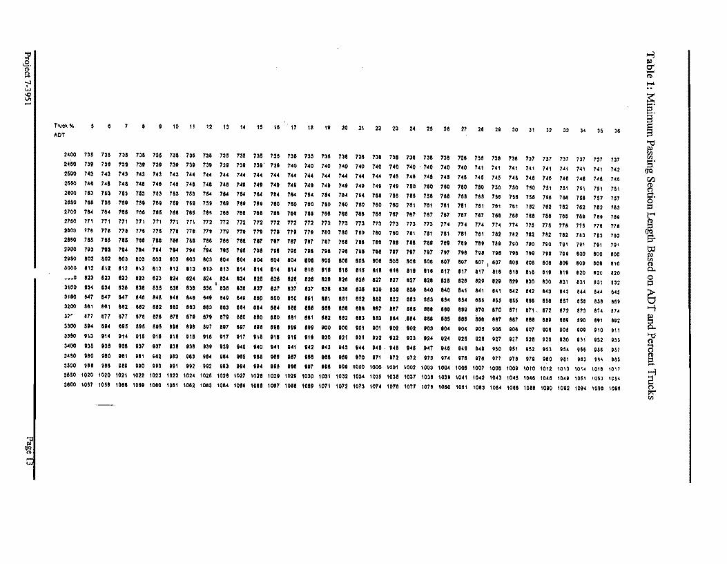
Table 1 Minimum Passing Section Length Based on ADT and Percent of Trucks 13
Table 2 Number of Passing Sections per 100 Kilometers on ADT and Percent Trucks 14
Table B-1 Service Rate (5.32 vehlmin) B-7
Table B-2 Service Rate (7.05 vehlmin) B-8
Table C-1 Number of Passing Lanes per100 km based onADT and Truck Percentage C-2
Table C-2 Lengths of Passing Lane for variable ADT and Truck Percentage C-5
Table C-3 Lengths of Diverge Taper, Ld, with respect to Design Speed and Lane Width C-6
Table C-4 Lengths of Lane Merge Taper, Lm, with respect to Design Speed and Lane Width C-8
Table C-5 Passing Lane Frequency for variable ADT and Truck Percentage C-10
Table D-1 Levels of Service and Maximum Service Volumes on Two-Lane Highways under Uninterrupted Flow Conditions D-7
Table D-2 Combined Effect of Lane Width and Restricted Lateral Clearance on Capacity and Service Volume ofTwo-Lane Highways with Uninterrupted Flow D-8
Table D-3 Truck Adjustment Factors for Each Level of Service on Different Terrains D-9
Table D-4 Passing Lane Length according to ADT and Truck Percentage D-34
Table D-5 Number of Passing Lanes per 100 kilometers according to ADT and Truck Percentage D-35
Table E-1 Traffic Count Summary Sheet on 07/17/98 Friday-Intersection at US 87 & 1879 (TX) E-5
Table E-2 Summary of Queue Formation on 07/17/98 Friday- Intersection at US 87 & 1879 (TX) E-5
Table E-3 Traffic Count Summary Sheet on 07/17/98 Friday US 64 before First Passing Lane E-6
Project 7-3916

Table E-4 Summary of Queue Formation on 07/17/98 Friday US 64 before First Passing Lane E-6
Table E-5 Traffic Count Summary Sheet on 07/18/98 Saturday-Intersection at US 87 & 1879 (TX) E-7
Table E-6 Summary of Queue Formation on 07/18/98 Saturday Intersection at US 87 & 1879 (TX) E-7
Table E-7 Traffic Count Summary Sheet on 07/18/98 Saturday- US 64 before First Passing Lane E-8
Table E-8 Summary of Queue Formation on 07/18/98 Saturday US 64 before First Passing Lane E-8
List of Figures
Figure 1 Existing Rural Two-Lane, Two-Way Cross sectional Geometric Section 2
Figure 2 Proposed Super-Two Cross Sectional Geometric Section 2
Figure 3 Super Two Benefit Cost Ratio vs. Average Daily Traffic 11
Figure 4 Super Two Benefit Cost Ratio vs. Truck Percentage 12
Figure 5 Case Study Map 15
Figure 6 Super Two Design for US 87 from Dalhart to Texline 16
Figure A-1 Type A Design with Continuous Interior Alternating Passing Lane A-7
Figure A-2 Type B Design with Separated Passing Sections A-8
Figure A-3 Type C Design with Overlapping Sections A-9
Figure A-4 TypeD Design with Isolated Passing Section A-9
Figure B-1 Queue in a Single Channel B-2
Figure B-2 Waiting Time vs. ADT (Service Rate= 5.32 veh/min) B-8
Figure B-3 Waiting Time vs. ADT (Service Rate= 7.05 veh/min) B-10
Figure C-1 Cross Section of a Rural Road in Texas C-12
Project 7-3916

Figure C-2 Cross Section for Texas Super Two
Figure C-3 Lane Configuration for Texas Super Two
Figure C-4 Signing and Pavement Marking for Texas Super Two
Figure C-5 Layout of Super Two sections from Childress to Hamlin for the Example Problem
Figure D-1 Current Two-Lane Rural Highway Cross-Section
Figure D-2 Proposed Super-Two Cross-Section
Figure D-3 B/C Ratio to ADT Levels
Figure D-4 B/C Ratio to Truck Percentage
Figure D-5 Number of Cars in Queue at Different ADT Levels
Figure D-6 Passing Lane Frequency
Figure D-7 Sensitivity of B/C Ratio
Figure D-8 Passing Lane Length
Project 7-3916
C-13
C-14
C-15
C-16
D-3
D-4
D-29
D-30
D-30
D-31
D-32
D-32
PROPOSED GEOMETRIC DESIGN OF TWO-WAY, TWO-LANE IDGHW AY INTERMITT ANT PASSING SECTION
(TEXAS SUPER TWO)
Introduction
Two-lane rural roads are of great importance in the American Highway System. There are more than 3 million miles (4.8 million kilometers) of two-lane rural highways in the United States, and they comprise about 97% of the total rural system and 80% of all U.S. roadways. It is estimated that 68 % of rural travel and 30 % of all travel occur on these rural two-lane roads. Funding is limited considering the extensiveness of the rural highway system and environmental concerns, and research for ways to improve the service of these roadways is essential. Because of the low ADT levels carried on these rural highways, low-cost improvement methods such as construction of Super sections are advantageous over the classical methods involving major modifications such as four-lane sections, extensive modification of road geometry.
The purpose of the study is to justify the implementation of intermittent passing lanes on rural two-way, two-lane highways where passing opportunities are limited. In this study, passing lane length and the distance between passing lanes are correlated to two major parameters: ADT and percentage of trucks. Passing opportunities are modeled to decrease with increasing oncoming traffic. In addition, as ADT increases, delay time savings increase. Also, the increase in the percentage of trucks creates more delay which results in a need for more passing lanes. A high percentage of trucks also causes operational problems in terms of reduced level of service, increasing passing attempts, aborted passes and driver frustration. An economic analysis is performed to reveal the benefit-cost ratios (B/C) for different situations. Reduction of queues and enhanced passing opportunities yield travel time savings and a predicted reduction in accidents. Taken together, these output parameters form the benefits accrued by implementing Super Two highway design.
Super Two geometry is essentially an attempt to provide improved highway capacity for those two lane rural highways whose ADT does not justify an upgrade to a full four lane cross section. This study used as its basis a typical two-lane highway cross-section of about 13.4 meters ( 44 feet) shown in Figure 1. Figure 2 depicts the Super Two cross-section that requires a widening of 60 centimeters (2 feet) to furnish a small shoulder on the passing side of the cross-section. Texas drivers are known to pull out onto the shoulder to let a faster moving vehicle pass on a rural road. Thus, the change to the Super Two cross-section essentially stripes the road the way Texas drivers actually drive it. The requirement for a shoulder is added to ensure that the economic analysis is conservative and comes from discussions with numerous TxDOT construction and maintenance engineers who feel that the shoulder is desirable as a protection for the pavement's edge.
Project 7-3951 Pagel

Shoulder
CJ
.. .. ... "" .. "" 3.00
...
Opposing Lane
~
3.70
D
.. ... ... ~
13.40 m
Traffic Lane
i
3.70
n
.. ~ .. ""
Shoulder
_.. ... 3.00
.. ...
Figure 1. Existing Rmal. Two-Lane, Two-Way, Cross-sectional Geometric Section.
Shoulder
~ ... ~ ...
3.00
... ""
... ....
Opposing Lane
~
3.50 .. ... ""
Passing Lane
i
3.25
13.60 m
... ...
Truck Lane
i
3.25
Figure 2. Proposed Super Two Cross-sectional Geometric Section.
Background
Shoulder
i .. .... .. ~
0.60 ..
_.. ...
The recent statutory change in the speed limit has had a dramatic impact on rural two-lane, twoway traffic. In years past, heavy trucks tended to utilize the interstate highway system because at the 55 mile per hour (mph) (88 klh) speed limit, it provided the least path of resistance. While actual distance driven were somewhat greater, trip times were roughly equal when compared to the use of rural highways owing to the delays encountered while driving through towns. The new speed limit changed that equation. By being able to travel at greater speeds, truck traffic can now realize a beneficial time saving by taking more direct routes to their ultimate destinations by using the rural highways. Thus, the percentage of truck traffic has increased. With this increase in large vehicles comes an increase in the number of passing movements required by passenger vehicles on rural highways. This condition is a direct function of the allowable speeds for the various types of vehicles. While passenger vehicles may travel at speeds up to 70 mph (112 klh), trucks are restricted to 60 mph (96 klh) and school buses are
Project 7-3951 Page2

required to drive no faster than 50 mph (80 k/h). This relative speed deviation creates a condition where drivers in open terrain like that in West Texas are tempted to execute potentially unsafe passing movements for three reasons. First, because the terrain is relatively flat they believe that they have the necessary passing sight distance when in many cases they do not. Secondly, because the traffic is generally light, they are more confident that they can execute this movement safely. Third and most critically for this study's purpose, they know that they must execute a passing movement at some point in time if they do not want to follow a slow moving vehicle to the next town because there are no alternatives.
This condition is further exacerbated by a driving behavior peculiar to Texas. It is customary in rural areas to pull over onto the shoulder and permit a faster moving vehicle to pass without having to pull completely into the oncoming lane of traffic. In fact, this practice has been carried to the point where a vehicle in the oncoming lane who sees a passing movement being executed ahead of it will also pull onto the shoulder, thus temporarily making a three-lane road out of a two lane one. While this certainly speaks well for the courtesy of West Texas drivers, this habit creates unsafe conditions in and of itself, not to mention the structural damage incurred to the paved shoulders. In order to change this driving habit, two conditions must exist. First, the driver must know that an opportunity to pass a slower moving vehicle will occur in a reasonable amount of driving time, and secondly, the driver must also know that the safe passing opportunity will occur independently from the status of oncoming traffic.
The ideal solution to this problem is to widen these rural roads and provide a four-lane highway. However, between $1.0 and $2.0 million per mile of construction cost, this is not economically feasible (Heimbach, et. al, 1974). The logical alternative is to determine at what volumes the additions of periodic passing lanes are justified, and develop several possible design alternatives to provide this capacity. Most states provide passing lanes on two-lane roads where passing sight distances are impossible to attain on hills and around long radius horizontal curves. Nevertheless, only a few have experimented with providing these lanes on terrain with adequate sight distances. New Mexico is one nearby state that has experimented with this concept. US Highway 64/87 between Raton and Clayton utilizes a Super Two style design (Eyler, et. al, 1996) with widened sections that permit passing at five to eight mile (8 to 13 km) intervals. Thus, passenger vehicles know that a passing section will be available every two to five minutes. A traffic study was conducted on that highway in New Mexico and its extension into Texas where no Super Two exists to verify that this change in highway geometry indeed enhances level of service. Details are contained in Appendix E to this report.
Several foreign countries have also taken a similar interest in enhancing the safety of their highways without incurring the construction costs of building four-lane highways. Appendix A to this report contains the details of intermittent passing lane design geometry currently in use in Canada, Mexico, and Germany. The recent enactment of the North American Free Trade Agreement (NAFT A) makes the study of the Mexican and Canadian Super Two standard designs very important. At this point in the study, it appears that the Mexican section will be most easily adapted to use in Texas. Considering the relative proximity of Mexico and the relative percentage of Mexican traffic as opposed to Canadian traffic, modeling the Texas Super Two design after the Mexican approach makes a lot of sense. The German design springs from a severe restriction on the amount of available right-of-way in European countries. Therefore, it
Project 7-3951 Page3

seeks to minimize the required cross-section. It only requires a total of 12 meters (40 feet) from shoulder to shoulder, but to achieve this, the Germans use only 0.25 meter shoulders (1 0 inch) and require a 0.5 meter (1.64 feet) separation between the opposing lanes traffic with a physical barrier if possible. This is not typical of the cross-section generally presented to U.S. drivers on rural roads. It will probably not only confuse them, but the virtual lack of shoulders would present a hazard in a stopped vehicle situation. The Canadian design uses two 1.2 meter ( 4 feet) shoulders while the Mexican design provides for a wider shoulder on the opposing lane side than on the passing lane side. This makes the most sense in that a vehicle breakdown on either side of the Super Two section will still leave sufficient room for one unobstructed lane in each direction.
A Mexican study of truck lanes was published in the Transportation Research Record (Mendoza & Mayoral, 1996) which indicated that benefits accrued from increased travel speeds as measured by the World Bank method outweighed the construction costs by as much as five times (Mendoza & Mayoral, 1996). Turkey has considered a similar scheme as an option to leverage scarce construction dollars while enhancing safety as that country builds its interstate highway system. Studies have also been done in Great Britain (McDonald, et al, 1994), China (Xing, 1989), and Australia (Oppy, 1992) regarding the provision of alternating passing lanes to both relieve congestion and enhance safety on two-lane roads with a high percentage of truck and bus traffic. The British study is particularly interesting in that one does not consider Britain as country with a lot of long rural roads. The motivation in that study was to minimize right-of-way acquisition cost in a country where available right-of-way is extremely rare and comparatively costly. Even this parallels the current environment in Texas, especially when one considers Super Two as a means to increase highway capacity within existing right-of-way limits.
This project had three major phases. First, a bench marking analysis of the literature, current TxDOT design criteria and cross sections, and assembly of appropriate standards for geometric design, signing/striping, and minimum traffic volumes was conducted. The output of this initial effort identified potential alternatives for providing this capacity that were evaluated in the next phase. It also estimated traffic volume justification criteria (maximum and minimum ADT's) which will permit this design to be a feasible alternative to four-lane highways. The second phase entailed a formal feasibility study to assess the costs and potential benefits of each of the various Super Two alternatives. Benefits and costs due to delay attributed to differential speed and headway were estimated using queuing theory (Khasnabis et. al, 1980). At the outset, a limited Monte Carlo simulation (Khasnabis et. al, 1980) was considered as a way to more accurately estimate delay savings benefits, but this was determined to be unnecessary as the ADT's involved did not justify themselves on a classically derived warrant basis. It was also found that Super Two could not be justified on delay savings alone. Accident savings had to be included and make up the majority share of the savings. Thus, a deterministic approach to calculating delay savings was determined to be adequate. The predicted values were then tested in a limited field traffic study on the case study highway to ensure that the deterministic model matched actual field observations. Details of the traffic study can be found in Appendix B. The fmal phase formalized the results of the first two phases by producing the necessary design documents to bring the concept to life on a test project. The documents include engineering drawings, signing, and striping plans are contained in Appendix C.
Project 7-3951 Page4

Application of Queuing Theory to Super Two Geometric Design
In order to model the traffic flow characteristics on a two-way, two-lane highway, queuing theory is applied. Queues are observed on that kind of highways when the opportunity to overtake a slow-moving vehicle is limited. The two basic components of queuing are arrival and service rate and their distributions. As traffic increases, the number of vehicles in a queue also gets larger because of increasing arrival rate and decreasing passing opportunities. Knowing these parameters, one can compute the average number of vehicles waiting to overtake the slowmoving vehicle. Light to medium traffic conditions on a rural roadway can be modeled using Poisson arrival distribution for the arrival rate. Assuming a negative exponential service rate distribution, expected number of vehicles in a queue (E(m)) and average waiting time (E(w)) for a vehicle in a queue can be calculated using equations I and 2 respectively.
2
E(m) - _q=---Q(Q-q)
E(w)- q Q(Q-q)
(1)
(2)
Where q is arrival rate and Q is the service rate, both tenns are expressed as the number of vehicles per unit time. As can be seen from equation 1, E(m), increases rapidly as the arrival rate increases or service rate decreases. Increasing ADT values on a roadway causes both the arrival rate to increase and service rate to decrease. In a situation where the arrival rate and service rates are close to each other, the queues tend to be infinite. This behavior of queuing theory makes the model applicable to simulate rural roadway traffic conditions. The average number of vehicles in a queue obtained from queuing theory is used for detennination of the passing lane length. Average amount of time spent in a queue is utilized to calculate the time savings that passenger cars will benefit from the construction of passing lanes.
Arrival and Service Rate Computation
A major difficulty in the application of the theory on a traffic problem is the dynamic characteristics of the traffic flow. The computation of the service rate (Q) should incorporate the fact that the truck percentage will have an influence on the service rate. Therefore, the service rate, Q, is computed using equation 3 (Highway Capacity Manual, 1987) below. This equation gives the maximum service volumes (SV), on rural two-lane, two-way highways under uninterrupted flow conditions. Service volume is then converted into service rate (Q) using a directional factor to fmd the service rate in one direction (in the case study a directional factor of 0.6 is assumed). Q values are further substituted into the equations 1 and 2. Unlike the service rate calculation, arrival rate, (q) is directly obtained from ADT values. Therefore, the arrival rate is an adjusted ADT value in one direction of roadway for a peak hour traffic volume. It is further assumed that the trucks are evenly distributed along the highway and they are not involved in passing maneuvers. Hence, the number of trucks are subtracted from ADT values during the calculation of the arrival rate.
Project 7-3951 PageS

SV = 2000 (vic) WL TL
Where:SV =Service volume (mixed vehicles per hour, total for both directions) vic = Volume to capacity ratio WL =Adjustment for lane width and lateral clearance at a given level of service T L = Truck factor at a given level of service
(3)
The truck factor (T L) and adjustment for lane width and lateral clearance (WL) are taken from the Highway Capacity Manual ( 1987). Volume to capacity ratio values are obtained from the Highway Capacity Manual (1987). A level of service ofB is assumed to simulate the mid volume rural conditions that are considered in this study. The volume to capacity ratio (v/c) is a function of the probability of a passing sight distance of 1500 feet (460 meters). Volume to capacity ratios are interpolated according to changing probability of having a passing sight distance of 1500 feet (460 meters). Since the roadway is on level terrain, the probability of having a passing site distance is 100 %. However, this probability will change according to the available gap between two vehicles in oncoming traffic. This gap will be a function of ADT level and the probability of having a gap equal or greater than 1500 feet (460 meters) is calculated using equation 4 assuming a Poisson distribution in oncoming traffic. Given that the probability of passing sight distance is 100%, the probability value obtained from equation 4 can be directly substituted into equation 3 to determine the service rate.
Where: A.= average number of vehicles in the opposing direction per unit time h = time gap between two consecutive opposing vehicles t = time gap between two opposing vehicles which are 1500 feet apart.
(4)
The average number of vehicles in the opposing direction per unit time (A.) is a direct function of ADT values. Equation 4 implies that as the traffic volume on a roadway increases, probability of having a time gap that will enable a safe passing opportunity will decrease. This decrease in the probability will reduce the service to capacity ratio obtained from the Highway Capacity Manual. Lower service to capacity ratios will cause a drop in the service volume or service rate. This theory is then extended to develop a design algorithm which optimizes both passing lane length and the distance between passing sections with respect to ADT and truck percentage. The details of this method can be found in Texas Department of Transportation Research Report TX-9817-3951-2R (Gransberg et. al, 1998) and are detailed in Appendix D. The method assumes that the optimum length of a passing lane is controlled by the time it takes the average queue to overtake the slow moving vehicle that has caused the queue to form. The optimum distance between passing sections is related to the time it takes for the queue to form behind the next slow moving vehicle. As a safety factor the design uses a length based on the average queue plus one car. As arrival rates are assumed to be modeled by the Poisson distribution, this provides an effective length that should permit safe passing for about 85% of the predicted distribution of queue sizes
Project 7-3951 Page6

Benefit-Cost Analysis
To justify the implementation of Super Two design on a public project, the benefits accrued by the design geometry must outweigh the cost of implementation. This is typically portrayed by dividing the equivalent annual benefit by the equivalent annual cost to compute the ratio of benefits to costs. If the resultant value is greater than unity, the project is economically feasible and warranted at the constraints imposed on the analysis by its underlying assumptions (Newnan, 1996). To complete such an analysis on Super Two highway design, the benefits are defined as the value of savings due to accident reduction and the value of time saved due to decreased delay. These benefits are computed as follows. Accident cost savings are obtained from the model provided by the equation 5 (Taylor and Jain, 1988). The constant 1.36 in equation 5 is used to convert 1988 dollars to 1998 dollars.
Bacc = (AC)(365)(ARF)(ADT)(l0-8 )(Lptloo)(1.36) (5)
Where Bacc Annual accident cost savings provided by a one mile passing lane ($/yr/mile); AC average cost of accidents by severity (value is taken to be $26,780 in 1988 dollars); and ARF = average reduction in accidents by severity for different ADT values (value is taken to be 37.7)
Time savings of the cars is the amount of time that can be accrued from the application of the design methodology. The value shows the amount of time that is saved by a car avoiding any waiting time behind a truck for a chance to overtake. The average waiting time per car, E(w) that had already been calculated from the queuing theory, Equation 2 is assumed to form the basis of time saving calculations. The major assumption is the elimination of this waiting time with the application of passing lane sections. In other words, with the application of passing lanes the cars are modeled to have an almost uninterrupted design speed. Time savings per vehicle per 100 kilometers (62.5 miles), (Btime) is annualized by multiplying them by ADT values and number of days in a year, 365 as shown in Equation 6. Number of trucks is excluded from the total number of vehicles since they don't benefit from time savings. The different time cost of business and leisure trips are incorporated in the calculations (Taylor and Jain, 1988).
Where:S10o =time saving benefits per 100 kilometers Sbt =time value of business trips Pb,= percentage of business trips S1, = time value of leisure trips P1, = the percentage of leisure trips ANp = average number of passengers passenger vehicle
Construction Costs
(6)
To calculate a corresponding construction cost per 100 kilometers (62.5 miles) of road, a conceptual design of the amount of roadway which must be upgraded to Super Two crosssectional geometry must be determined. Additionally, it is assumed that the upgrade will consist of an average widening of 60 centimeters (2 feet). It should be noted that if the specific project in question is determined to not require a small shoulder on the passing lane side, then the cost of
Project 7-3951 Page7
implementing Super Two geometry is merely the cost of new signage and striping. The conceptual design begins with determining the effective length of a Super Two passing lane. An effective length of passing lane is long enough for the drivers of the passenger cars to feel comfortable overtaking the slower moving truck. There should also be enough length provided for the trucks to merge into the passing lane. Tapered sections at the beginning and end of the passing lane would effectively provide this space. But the tapered sections would not be included in the length of the passing lane. The tapered sections should be equal to the distance traveled by the truck as it moves into and out of the passing lane safely clearing the passenger cars in the queue.
Lepl = (t ace + f pl )~,
Where:Lept = Effective length of passing lane (meters) tacc = Time for a passenger car to accelerate (seconds) tp1 = Time for platoon in queue to pass (seconds)
(7)
The distance from the point where a car overtakes the first truck to the point where it reaches the next truck is considered as the distance between two passing lanes, (Dpl) as shown in equation 8. Assuming an even distribution of the trucks and trucks will cause no delay for cars, this length also includes the passing lane section of the highway. Ideally the passing lanes are designed to be located at the points when cars reach the next slow moving truck. It is assumed that the queue with an average number of cars, E(m) would be formed by the time the platoon reaches th~ next passing lane.
Where:Dpt =distance between passing lanes (meters) V tr = truck speed; qtr = truck arrival rate V pc = passenger car speed ~ V pc-tr = differential speed between truck and passenger car
(8)
The calculated values for the length and the separation of the passing lanes will be converted into a representation per a reference basis. For practical purposes presenting the values in a per distance basis is more meaningful. Therefore an interval of 100 kilometers (62.5 miles) is selected to form that basis. Equation 9 represents the number of passing lanes per 100 kilometers (PL10o). Since, the distance between passing lanes has already been calculated, the number per 100 kilometers is obtained by dividing 100 kilometers to distance between passing lanes. It should be kept in mind that this distance includes the passing lane length and the result will directly give the number of passing lanes per 100 kilometers. Total length of the passing lanes per 100 kilometers can also be calculated after the number of passing lanes per 100 kilometers (Lpnoo) is shown in Equation 10.
Project 7-3951 Page 8

(9)
(10)
Construction cost per 100 kilometers of roadway section, Cpb is found from Equation 11 by multiplying by two since the passing lanes in the opposing direction must be considered. The length of merge and diverge areas is not a function of length of passing lane.
C = 2(uc p!Lep/loo + UC PL J ~ 1000 ~ 100 (11)
Where: UCp1 = Construction cost of 1 kilometer of passing lane UCcd =Construction cost of converge and diverge sections per each passing lane
The construction cost is a one-time cost that occurs at the beginning of the project. It should be incorporated in the economical analysis in annual basis so that comparison of the cost and benefit values can be done. Equation 12 annualizes the construction cost of the passing lanes using a life cycle ofn years and an interest value i. Life cycle period of the project should be estimated according to the characteristics of the roadway.
(12)
(A \P, i%, n) = Capital recovery factor for an interest value of i% and for n years
Case Study-Parametric Calculations of Time Savings
A case study using actual data from Highway 87 between Dalhart and Texline in Dallam County, Texas is presented in the following sections to exemplify the proposed equations. The most critical ADT level of 3600 vehicles/day is chosen for the example. Each formula presented in the previous section will be calculated based on assumed parameters. Various calculations for different ADT and truck percentage levels are presented in this report. The design speeds for the passenger cars and slower moving trucks are decided to 70 mph and 60 mph, respectively. However, for the sake of metric unit calculations their speeds are taken as 112 k/h and 96 k/h, respectively. A representative truck percentage of 10% is chosen for this specific case study. The upgrade of the existing roadway to a 3-lane pavement with a passing lane is planned with a 60 centimeter pavement widening as shown in Figure 2. Since the structural capacity of the existing 3-meter (10 feet) shoulders is the same with regular lane sections, shoulders should be kept as they are. The 60 centimeter (2 feet) new construction is foreseen with the same structural capability of present pavement. The existing and proposed sections are comprised of a 0.6 meter (2 feet) flexible subbase, a 0.6 meter (2 feet) fly ash base, and a two course surface treatment
Project 7-3951 Page§

After the pavement is extended 60 centimeters (2 feet), a final seal coat application is designed to cover existing markings. This prepares for the striping of new pavement markings. Another construction activity would be the merge and diverge areas or the tapered areas of the passing lanes. The cost of these areas does not depend on the length of the passing lane. The approximate construction costs are as follows.
• A two-course surface treatment with AC-5, Grade 4 aggregate is needed on the new shoulder. Application rate of binder is 2 11m2
, and distribution rate of aggregate is 137 m2/m3
• It is calculated to be $1,020/0.6m width/lkilometers length. • A one-course seal coat application with AC-5, Grade 4 aggregate is needed across the
entire cross section. The application rate of binder is 211m2, and the distribution rate
of aggregate is 137 m2/m3• It is calculated to be $12,309113.80m width/lkilometers
length. • Fly ash stabilized base construction cost is calculated to be $9,000/0.6m
widtb/lkilometers length. • Flexible subbase construction cost is calculated to be $6,000/0.6m width/1kilometers
length. • Excavation cost is $1,391/0.6m width/lkilometers length. • Embankment cost is $1,1 05/0.6meters/1kilometers length. • Cost of diverge and converge areas is $1,222 I 0.6meters width/passing lane. • Total cost excluding signing cost is $30,825.
The analysis shown in Figure 3 is performed at a constant truck percentage of 10% and with varying ADT levels. The B/C ratio increases with increasing ADT levels. The Super Two Highway can be justified from an ADT level of2500. This justification is mainly caused by the accident cost saving benefits. The equation used in this calculation can be further elaborated or examined to conform to the actual accident cost saving analysis specifically conducted for a roadway section. It is evident that time saving benefits are not adequate to justify the construction of the Super Two Highway (approximately 15% of the savings are contributed by the time saving benefits). However, the construction cost pertaining to the upgrading of the highway is primarily widening cost. Many people with highway construction experience agree that widening is not a necessity. For the segments of the highway with passing lanes, striping will be adequate for safe traffic conditions. The cost of striping is much less than construction cost. If highway agencies can adopt this idea, the construction of passing lanes at given intervals will be a viable solution to the improvement of the two-way two-lane rural highways.
Project 7-3951 Page IO
1.80 1.60 1.40
0 1.20 i= 1.00 <{ a:: 0.80 (.)
• • • • • • • • • • • • • • • • • • • • • • • • • - 0.60 CD
0.40 0.20 ··--·
0.00 2000 2200 2400 2600 2800 ADT 3000 3200 3400 3600 3800
Figure 3. Super Two Benefit Cost (B/C) Ratio versus Average Daily Traffic (ADT).
It is evident that, time saving benefits are not adequate to justify the construction of the Super Two section (approximately 15% of the savings are contributed by the time saving benefits). However, the construction cost pertaining to the upgrading of the highway is primarily widening cost. Many people with highway construction experience agree on that widening is not a big necessity and they think that for the segments of the highway with passing lanes only striping will be adequate for safe traffic conditions. The cost of striping is much less than construction cost, ifhighway agencies can adopt this idea then construction of passing lanes at given intervals will always be a viable solution to the improvement of the two-way two-lane rural highways.
Another outcome of the constant ADT and changing truck percentage analysis is the B/C ratio is not sensitive to truck percentage. This is caused by the structure of the accident cost benefit equation. Figure 4 is plotted for a constant ADT of 3600 and varying truck percentage. An almost constant line is observed. This is because accident cost savings included in the numerator and construction costs included in the denominator are both functions of the passing lane length, and therefore cancel each other out. This leaves a constant B/C with respect to truck percentage.
Project 7-3951 Page 11

0 +=> ('(!
a::: () -m
2 1.8 1.6 1.4 1.2
1 0.8 0.6 0.4 0.2
0 0 5 10 15 20 25 30
Truck Percentage
Figure 4. Super Two Benefit Cost (B/C) Ratio versus Truck Percentage
Designing the Super Two Section
35 40
The previous equations are drawn from a more detailed derivation contained in Appendix D. This analysis optimizes both the length of passing section and the number of passing sections per 100 kilometers ( 62.5 miles) of highway with respect to cost. For this analysis, a passing section is defined as provision of passing lanes for both directions of travel. It can be seen in Appendix A that there are four basic types of Super Two sections. In Type B, Separated Passing Sections, the engineer will need to be careful to ensure that there is a passing section developed for both directions. At this point, the design methodology is very simple and straightforward. Its steps are as follows.
1. Determine the ADT and percentage of trucks for the highway in question. This can be based either on existing traffic data adjusted for future growth or from another more appropriate method or policy.
2. With this input data, enter Tables 1 and 2, and determine the number of passing sections per 100 kilometers (62.5 miles) and the minimum length of each passing section.
3. Taking plan and profile information for the highway in question, determine those portions of the road where safe passing sight distance is not available due to horizontal curves, vertical curves, and other obstructions.
4. Allocate Super Two passing sections to roadway sections where passing site distance is unavailable.
5. Distribute any remaining passing sections evenly between the passing sections already allocated.
6. Taking the average passing section length from Table 1, adjust as necessary for those sections without adequate passing sight distance to provide safe passing throughout the length of the sight distance restriction.
Project 7-3951 Page 12
TI\ICl<%
AOT a 0 10 11 12 13 14 18 10 < 17 18 10 20 21 22 23 24 25 20 27 21 20 30 31 32 33 3~ 3$ 35
2400 735 735 735 735 738 735 735 735 735 735 738 738 738 735 735 73e 73e 738 738 730 738 738 738 730 730 730 737 137 737 737 737 737
24SO 730 730 730 730 730 730 730 731 730 731 730' 730 740 740 740 740 740 740 740 740 , 740 740 740 741 741 741 741 741 741 741 741 742
2&00 743 743 743 743 743 743 744 744 744 744 744 744 r44 r44 744 r44 744 744 74& 748 745 r45 745 745 145 745 748 740 748 740 7411 145
2550 740 74e 748 748 748 748 748 748 748 740 74t r4t 740 r4t 740 r4t r40 740 r4o 780 r8o 780 780 780 750 750 750 751 751 751 751 751
2800 753 rn 7&3 753 763 753 783 7!4 714 784 784 784 784 754 1e4 ru 754 rea 75& 755 758 rea ru 755 758 758 1so 758 75o t5e 757 757
2850 788 750 < 780 710 750 750 750 750 780 781 780 780 780 780 780 780 780 780 700 701 701 701 781 781 781 781 782 702 7112 702 702 753
2100 784 1u ree roe 1ee rae 785 785 ree 78e 78e ree ro11 rea 788 7e8 7ee rea 101 101 767 787 nr r11r rea 7118 rea 781 ree 100 reo 1eo
2750 771 771 t71 771 771 t71 7t1 772 772 772 772 772 r72 rr2 773 773 773 773 773 773 r73 774 774 774 774 774 775 775 775 775 775 775
2800 715 778 778 778 778 771 771 770 770 771 771 770 77t 770 710 780 780 780 780 711 781 781 781 781 782 782 782 782 782 783 783 783
2850 785 us 785 788 788 tee tee rae reo tee 787 787 787 787 111 rea 1ee 7ee rae rae 7&0 7eo 7U 780 tn roo 1oo 100 101 101 a1 101
2000 t03 703 704 704 704 704 704 io4 ros ro6 705 708 7ts roe 718 roe roe roe 11r 707 rn 111 ne 7u 708 708 110 100 1u 800 8oo 100
2050 ao2 ao2 eo3 1103 1103 eo3 1103 ao3 eo4 804 ao4 &04 804 805 ao5 80S eo5 ao8 eoe ao8 aoa ao7 aor 807 1
1101 808 ao5 11011 aoo 5oo eo9 110
3ooo e12 e12 812 112 eu a13 813 813 &13 814 814 814 814 e1e 818 1118 au 81& 11111 118 11u 1111 817 111 au 1111 e111 1111 110 820 120 120
•• ~o 823 1123 1123 1123 1123 824 824 &24 e24 824 e2s e2e e2e 128 112e 8211 8211 827 827 82r 11211 828 11211 uo 820 1120 ,83o a3o u1 831 831 n2
3100 834 834 1138 8311 835 11311 83e e311 I 8311 838 83r 837 83r 837 838 113e 838 830 1130 830 840 840 1141 841 1141 542 842 843 843 844 844 045
31110 847 847 1147 11411 &411 11411 148 1140 s4o e4o a&!l 1150 e5o a&1 118\ e111 1152 n2 es2 ee3 853 U4 &54 1155 ass 855 a5e 11511 est 858 858 859
3200 8111 11111 ae2 ae2 1182 882 583 ee3 11113 1184 eu 11114 885 see eea see eee ear 11111 eee eea 8ao sao no aro 1111 8t1 . a12 an an 874 81.1
3'', ett 877 en a1e 87e e7a no e1o a1o uo 11110 eeo ea1 ee1 11112 ae2 ee3 ee3 ee4 ,8114 eee ee5 8118 see ea7 ae1 see aao a eo 1100 1191 102
3300 au at4 eos au 505 aoe eoe so1 ao7 807 eoe eoe aoo aoo ooo ooo 101 001 002 002 003 004 804 oo5 oo11 ooe oot ooa oo5 oo9 010 911
3350 813 014 014 018 018 015 81e 0111 017 017 0\8 018 010 010 020 021 021 022 022 023 024 024 025 0211 027 027 0211 020 030 03f 032 033
3400 035 035 035 037 037 038 038 030 030 040 040 041 041 042 043 043 044 045 < 046 0411 047 0411 040 940 050 051 052 853 054 055 0511 057
3450 080 080 oe1 081 oe2 083 oe3 oe4 oe4 oe5 0811 08e oar oae oee oeo oto 011 or2 012 073 074 0111 078 on ote 010 oeo 981 oe3 u~ oas
35oo ou oe8 oeo ooo ooo oo1 eo2 oo2 903 oo4 004 oos oo8 001 ooe ooo 1000 1000 1001 1002 10o3 1004 10011 1001 10011 1000 1010 1012 1o13 1ou 10111 1011
3550 1020 1020 1021 1022 1023 1023 1024 1025 \02e 1027 \0211 1020 1020 1030 1031 1032 1034 1035 10311 \037 10311 1030 1041 1042 1043 1045 10411 10411 1040 1051 1053 lOS~
31100 105t 10511 10811 1050 10eo 10111 10112 10113 10114 108& 10ee 10117 10118 10110 \071 1072 1073 1074 \07e 107t \Ota 10110 10111 1083 1084 10IIe 10118 1000 1002 \004 1000 1000

Truck y,
AOT 2400
2460
25!10
2800
2860
2700
2760
2800
2850
2000
2950
3000
3050
3100
3160
3200
3250
3300
3350
~00
~50
3500
3550
3800
2
2
2
2
2
2
2
2
2
2
2
2
2
2
2
2
2
2
2
2
2
2
2
2
2
8
2
2
2
~ 2
2
2
2
2
2
2
2
2
2
2
3
3
3
3
3
3
3
3
3
3
7
2
2
2
2
2
2
3
3
3
3
3
3
3
3
3
3
3
3
3
3
3
3
3
3
3
8
3
3
3
3
3
3
3
3
3
3
3
3
3
3
3
3
3
3
4
4
4
4
4
4
4
0
3
3
3
3
3
3
3
3
3
3
3
4
4
4
4
4
4
4
4
4
4
4
4
4
4
10
3
3
3
3
3
4
4
4
4
4
4
4
4
4
4
4
4
4
4
4
6
5
5
5
5
11
4
4
4
4
4
4
4
4
4
4
4
4
4
4
5
5
5
6
6
6
5
5
5
5
5
12
4
4
4
4
4
4
4
4
5
5
5
5
5
5
5
6
6
6
II
II
5
8
8
8
8
13
4
4
4
4
5
5
5
5
5
5
5
5
5
5
6
&
8
8
8
8
8
8
8
8
8
6
5
li
5
5
5
li
5
li
5
li
8
8
8
8
8
8
8
8
8
8
8
7
7
7
16
5
5
li,
6
II
5
5
8
8
8
8
8
8
8
8
8
8
7
7
7
7
7
7
7
7
16
5 5
5
5
8
8
8
8
8
8
8
8
8
7
7
7
7
7
7
7
7
7
8
8
8
17
5
e 8
8
8
8
8
8
8
8
7
1 7
7
7
7
1
7
8
8
8
8
8
8
8
18
8
8
8
8
8
8
7
7
7
7
7
7
7
7
7
8
8
8
8
8
8
8
8
9
9
19
8
8
8
8
7
7
7
7
7
7
7
8
8
8
8
8
8
8
8
9
9
9
9
9
9
20 21
8 7
7 7 7 7
7 7
7 7 7 7
7 8
7 8
8 8
8 8
8 8
8 8
8 8
8 9
8 9 8 9
9 9
9 9
9 9
9 9
9 10
9 10
9 10
10 10
10 10
22 23
7 7
7 8
7 8
8 8
8 8
8 8
8 8
8 8
8 9
8 9 9 9
9 9
9 9
9 9
9 10
9 10
9 10 10 ' 10
10 10
10 10
10 10
10 11
10 11
10 11
11 11
24
8
8
8
8
8
9
9
9
9
9
9
9
10
10
10
10
10
10
11
11
11
11
11
11
12
25 26 27
8 8 9
8 9 9
8 9 9
9 9 9
9 9 9
9 9 10
9 9 10
9 10 10
9 10 10
10 10 10
10 10 10
10 10 11
10 10 11
10 11 11
10 11 11
11 11 11
11 11 12
11 11 12
11 11 12
11 12 12
11 12 12
12 12 12
12 12 13
12 12 13
12 13 13
28 29 30
9 9 10
9 10 10
9 10 10
10 10 10
10 10 10
10 10 11
10 10 11
10 11 11
11 11 11
11 11 11
11 11 12
11 11 12
11 12 12
11 112 12
12 12 12
12 12 13
12 12 13
12 13 ' 13
12 13 13
13 13 13
13 13 14
13 13 14
13 14 14
13 14 14
14 14 14
31 32
10 10
10 11
10 11
11 11
11 11
11 11
11 12
11 12
12 12
12 12
12 12
12 13
12 13
13 13
13 13
13 14
13 14
13 . 14
14 14
14 14
14 15
14 15
15 15
15 15
15 15
33
11
11
11
11
11
12
12
12
12
13
13
13
13
13
14
14
14
14
15
15
15
15
15
18
16
34 35
1 1 11
11 11
11 12
12 12
12 12
12 12
12 13
13 13
13 13
13 13
13 14
13 14
u 14
14 14
14 15
14 15
15 15
15 15
15 15
15 16
15 18
18 16
16 16
HI 11
16 17
36
12
12
12
12
13
13
13
14
14
14
14
14
15
15
15
15
16
16
16
HI
17
17
17
l7

Case Study Design Example
Oklahoma r··----··-·---·-··-··-··-··--·-·--··-··--·--·----------··-
~exline I ADT = 2400 j
Clayton, NM
I ADT= 3600
New Mexico 1727
Dalhart
Figure 5: Case Study Map
Figure 5 shows the details of the case study area. This is also the area on which the traffic study was conducted to validate the deterministic queuing model on which the design methodology is based. The ADT volumes come from the current Amarillo District traffic map. As ADT ranges from 2400 to 3600, a Super Two design is warranted as minimum ADT is greater than or equal to 2400.
For purposes of illustration only, let us assume that design ADT will equal 3 600 with 1 0 percent trucks. Using Table 1, we find that the average length of the passing section will be 1061 meters. From Table 2, we find that 5 passing section per 100 kilometers are warranted. The distance is 62 kilometers; therefore, the number of sections must be adjusted as follows.
Actual number of sections= 62 km (5 sec) = 3.1 => 3 passing sections lOOkm
Thus, the engineer must distribute three Super Two sections along the road between Dalhart and Texline. As this highway runs between two population centers, the first passing section will be a Type A split with the westbound half exiting Dalhart and the eastbound half exiting Texline. This permits those passenger cars that catch the slow moving vehicles in town due to the slower speeds to take advantage of their faster acceleration to highway speed and avoid forming queues immediately outside of the two towns. That leaves two passing sections to be distributed between the two towns. The priority would be to place these at locations where passing sight distance is inadequate. To minimize construction costs, these remaining sections would be Type B, Separated Super Two sections. They would be roughly 20 kilometers apart. Figure 6 is an idealized depiction of the final design layout.
Project 7-3951 Page 15

1.06 km
- 18 km __ ___,.,..,.
1.06 km
1.06 km
-18 km
1.06 km
1.06 km
- 18 km -----'.,..,..
1.06 km
Texline
TYPE A Texline Half
TYPEB Separated Section
TYPEB Separated Section
TYPE A Dalhart Half
Dalhart
Figure 6. Super Two Design for US 87 from Dalhart to Texline.
Project 7-3951
-62 km
Page 16
Field Traffic Study of Case Study Area
A short traffic study was done on the case study area in July 1998 to compare the actual observed effect of Super Two geometry to the effect computed in the deterministic queuing model. The observed peak hour volume on July 17, 1998 was 532. The average number of vehicles for the same hour is counted as 3.00 according to Traffic Count Summary Sheet (Table E-1). The same parameter can be found from the design method as described earlier in the Case Study portion of the report. The peak hour corresponds to an ADT of 3 54 7 by using a peak hour factor of 0.15. As a result, the average number of vehicles per queue calculated by the deterministic queuing model for the case study is 3.15 vehicles per queue. This result validates the model and the design approach of basing passing lane length and spacing on an average predicted queue plus one.
The traffic study also validated the hypothesis that implementing Super Two would greatly enhance level of service on low volume rural highways. From Table E-6, one observes that the average number of vehicles in queues going towards North at the data collection point in Texas is 3.54. Whereas, the same parameter becomes 2.40 after vehicles cross Clayton where the effect of Super Two passing lane sections occur. The reduction rate is 32 percent. In the other direction, the following numbers are observed. In New Mexico, the average number of vehicles in queue is 1.81 (Table E-8) for the vehicles leaving the passing lane where this number has direct effect of passing lane. The same parameter becomes 3.73 in Texas (Table E-6). Then, the corresponding reduction rate in the average number of vehicles in queues due to Super Two is 52 percent. Thus implementing Super Two can be concluded as having a strong positive impact on traffic flow.
Conclusions
A number of interesting conclusions can be made. This methodology can be used to justify the Super Two Highway at ADT levels less than 4200 vehicles per day. A Super Two section that requires a 60-centimeter widening is economically feasible at ADT levels greater than 2400 vehicles per day. If no widening is required (i.e. no shoulder on passing section side), then Super Two is economically justified at much lower ADT levels. Super Two B/C ratio is insensitive to truck percentage. Typical queues will contain less then four vehicles. Designing for the number of passing lanes per 100 kilometers of road provides high design flexibility without introducing significant error. If ADT levels exceed 4200 vehicles per day, the passing lane design should be based on simulations or other appropriate urban design methods.
It should be noted once again that 0 to 4200 vehicles per day is the ADT range where the feasibility study is applicable. After a certain level of ADT, waiting times of the passenger car in the queue become very large and then the values drop below zero. This drastic change in the values is caused by the characteristic of queuing theory. The theory is valid for the arrival rates (q) less than service rate (Q). However, the research model has increasing arrival rates with ADT, and service rate decreases as ADT values become larger because of the physical limitations of the highway. The point where two values intersect there is an infinite queue. This is obviously not an appropriate situation for the rural highways. The limiting ADT value for the application of the model is 4200. For the upper traffic levels other techniques like simulation programs may be used to model the real traffic conditions. This kind of method, however, is not in the scope of this research.
Project 7-3951 Page 17

The combination of the traffic study in New Mexico and the results of the deterministic model, validate the design methodology detailed in this report. The economic justification comes not from delay savings, but from the savings accrued by a reduction in accidents. However, when the section is implemented, additional savings will be accrued due to enhanced level of service. These savings are not included in the model. Therefore, the model is a conservative approach to this issue.
Finally, it must be remembered that the model developed in this study assumes a required widening of the standard 13.4 meter (44 feet) cross-section to 13.6 meters (46 feet). The determination of the requirement for a shoulder on the passing lane side of the road is a judgement call that should reflect actual conditions for each individual project. There are numerous examples of slow moving vehicle passing lanes throughout the State of Texas where no shoulder is provided. If this can be done, Super Two is economically justified at much lower ADT's than those shown in economic analysis of the model. One could argue that if project conditions permit the use of no shoulder, Super Two could be implemented for the cost of a seal coat, new striping, and new signage. Therefore, the Department could accrue significant benefits due to increased level of service and decreased accidents at very little cost.
Recommendations
We have two recommendations as a result of the above discussions. First, the Department should implement Super Two as soon as possible. It provides a means to upgrade level of service on highways that cannot justify an upgrade to a four-lane cross-section. It also enhances safety for the traveling public at very little incremental cost. Secondly, the Department should survey its major rural highways and identify those that could be upgraded to Super Two without the requirement for a shoulder. These roads could be systematically converted to Super Two geometry in conjunction with the districts' annual seal coat contracts. The only additional expense would be a slight increase for striping and the cost of resigning the Super Two sections. This is an opportunity to immediately implement the results of this research.
Project 7-3951 Page 18

APPENDIX A: LITERATURE REVIEW
Introduction
In recent years there has been an increasing interest in the operation of two-lane rural and suburban roadways. Increase of traffic volume and reduced funding levels are some of the primary reasons behind it. The recent statutory change of speed limit causes a significant impact on rural two-lane, two-way traffic. The new speed limits of 70 mph for passenger vehicles, 60 mph for trucks and 50 mph for school buses have changed the flow of traffic through these rural highways. Trucks are now using these rural highways for higher speed limit (which was 55 mph) and shorter travel distance. This increase in traffic volume and differential speed limit causes drivers to take potentially unsafe passing maneuvers. The flat terrain of West Texas is also working as a catalyst to that. Now there is a growing need to maximize capacity, mobility and safety of existing two-lane highways.
One way to solve the problem is to provide four lane highways. However, The cost of construction, $1.0 to 2.0 million per mile, is not economically feasible. That's why the "Super Two" concept comes into the frame with a median to provide passing facilities alternately. The access to this median will be controlled according to the flow of traffic.
The concept of Super Two is not totally new. There are many roadways that meet super two requirements such as two-lane freeways that have been built, either as a first stage or as a final product. These versions of the Super Two usually have been considered only as interim steps to full four-lane freeways. Some of the key features of the Super Two are full width lanes, full width shoulders, frequent passing lane locations and the extensive use of right turn lanes, left turn lanes, and continuous left turn lanes. Therefore the Super Two will provide facilities of a four-lane highway with low construction cost.
Definition
Super Two refers to a freeway or controlled access at-grade roadway with a single through lane per direction. The idea behind Super Two is to increase the capacity and safety of the existing two-lane two way highways.
The key elements of a Super Two Highway are listed below.
1) Full width lanes, paved shoulders and clear zones 2) A center passing lane 3) Limited access, with turn lanes for all permitted turns 4) Horizontal and vertical curves with high speeds 5) Passing lanes, speed differential, and truck lanes 6) Provisions for expansion to freeway or divided roadway 7) Proper interchange design for a two-lane freeway
For a new facility to be classed Super Two, most guidelines should be met. For upgrading an existing roadway, these defining features can serve as a menu of improvements for consideration.
Project 7-3951 Page A-1

Project Objective
The objective of this project is to produce a standard methodology to design and to construct a Super Two highway. This means to modify the existing two-lane two-way highways to a Super Two highway. This goal will be achieved in three phases. In the first stage, reviews of literature, TxDOT design criteria, and cross sections and standards for signings and striping have been accomplished. The result of these reviews and studies is the design alternatives we set for further discussions. The next phase will be the cost-benefit analysis for the different design alternatives and ADT's for these roadways. In order to find the cost of delay, an analytical technique involving queuing .theory will be implemented at this phase. The possible two or three design alternatives will be decided from the outcome of this analysis. The third and the final phase will be to summarize the results of the above two phases with necessary design documents and drawings to be implemented into a test project. This will be arranged with engineering drawings, cross sections, passing lane design details, signing, and striping. The documents will include proposed traffic volume criteria, cost estimation information and a formal constructibility review for each design alternative.
Design Philosophy
The philosophy of Super Two is to provide smooth traffic movement and overtaking maneuvers in the traditional two-lane two-way highways. If constructed as a two-lane freeway, the Super Two will provide the facilities of a four-lane at-grade roadway. In planning a regional road system, the Super Two would be a type of facility that would typically be used for minor arterials and volume principal arterials.
Design Features
Two-Lane Rural Highway
lr--3 oooc--+I~ 3. ;ooo-' ~~----· 3 700o-----i-J """J ~~------------134000-------------
The basic two-lane highways have two middle lanes of3.7 min each direction (as shown in the above figure) and shoulders of3.0 m each. That makes the total width of the highway 13.40 m, and cross slope is 2%. There is no passing lane in it, and shoulders are designed fully surfaced.
Project 7-3951 Page A-2

Design Speed
The Design Speed for Super Two should range from 80 to 110 kmlh when an existing two-lane highway is upgraded to Super Two. In all new construction and reconstruction, the Design Speed of 100 to 110 kmlh should be used throughout (Minnesota DOT). In all cases, when upgrading the existing roadway, the designer should apply the speed that is greater than or at least equal to the posted speed.
Average Daily Traffic
The ADT value of 2000 is considered to be the critical ADT between two and four lane highways. In a study published in the Transportation Research Record (TRR) 1303, "Warrants for Passing Lanes", shows that Passing Lanes on rural two-lane highways have favorable benefit/cost ratio at ADT's of 6500 and greater.
The length of a passing lane is dependent on the volume of vehicles per hour (vph) for the project. The optimal length of passing lanes to reduce platooning is 0.8 to 1.6 km (Minnesota DOT). A general guideline for the development of design length is as follows.
Vehicles per hour (vph) one way 400 700
Length of passing lane 1.2 to 1.6 km 1.6 to 2.0 km
The spacing design for a passing lane is dependent on traffic volume. For a vph ofless than 700, this spacing may vary from 16 to 24 k.m. On the other hand this spacing may vary from 5 to 8 km or even more frequent for a vph of 700 or more.
The three-lane section consists of an added lane in the middle to provide passing facilities in alternate directions. This change of direction of the middle lane may be uniform or traffic actuated, depending on situation. The center lane added to the two-lane section is of the same width or a bit different than that. The shoulders of a three-lane section may be narrower than that in the two-lane section, as being practiced in Germany, Canada, Mexico, Turkey, and some other countries of the world. Brief description of the German, Canadian and the Mexican cross sections are as follows.
Project 7-3951 Page A-3

Three Lane Highway Cross Section in Canada
J I 1\
\l!
I
- .0000 L3 6000 3 7000 i 3 7000 1. 2000
1 3. 4000
The design consists of two 3.7 m lanes and a 3.6 m lane with shoulders of 1.2 m each. The direction of passing will have a 3.7 m and a 3.6 m lane as shown in the above figure. The total width of the highway remains 13.40 m.
Three Lane Highway Cross Section in Germany
I r-M rh r-
I
\ 3. 7500 I \ 3 7500 3.5000 \
o. 2500 0.5000
I
~----------------------------12 0000----------------------------~
In Germany, the highway is designed with two 3.75 m and one 3.5 m lanes. The middle lane of 3.75 m width is provided to facilitate passing in alternate directions shown in figure. The curbs are of0.25 m each making the width of the highway as 12.0 m. This design is suitable for an ADT less than 2000. Overtaking is prohibited in the opposing lane.
Project 7-3951 Page A-4
0. 2500

Three Lane Highway Cross Section in Mexico
Possi r_jE'('
i Dovbl e I Borri er ~i ne V
I I II I
I
I il I
-- 1 5000 !i . 35000 \'
35000 3.5000 .. I{. \
~ IJ. 8000
Lo. 1000 L C:. 4000 Lo.lOOO .'-0 lfCO
~----------------------------135000----------------------------~·
This design alternative practiced in Mexico consists of three equal lanes of3.5 m each with a central median of0.4 m. Here the shoulder in the direction of passing is limited to 0.8 m and that on the reverse direction is 1.5 m as shown in figure. This change in shoulder width may provide some added safety to the driver.
Previous Benefit-Cost Analyses of Super Two Highways
The growing need for the two-lane highways with more capacity, mobility, and safety has lead researchers to put emphasis on alternative designs. On the other hand, limited funding and environmental issues are big concerns in opening new corridors to handle heavy traffic flows. As a result, the Super Two concept has recently started drawing more attention.
There are more than 3 million miles of rural highways in the United States; this figure represents about 97 percent of the total rural system and 80 percent of all U.S. roadways. It is estimated that about 68 percent of the rural transportation and 30 percent of all travel in U.S. is done on the rural two-lane system.
The major benefits of a passing lane are reductions in delay and accidents. In order to evaluate the effectiveness of the passing lanes, the cost savings of the motorists over a wide range of traffic volumes and the construction and· maintenance cost of the passing lanes should be compared. The reduction in delay provided by a passing lane results in operational cost savings to the road users. A unit value of time that is usually expressed in dollars per traveler hour is multiplied by the amount of time saved in order to compute the time cost savings. Furthermore, besides the needs for updating these values to current price levels, travel time value is sensitive to trip purpose, travelers' income levels, and the amount of time savings per trip.
Project 7-3951 Page A-5

According to AASHTO, the time savings is divided into three categories and can be expressed as a function of time saved in a trip and type of a trip.
1. Low time savings (0-5 min): For work trips and average trips, the values of time per traveler hour are suggested as $0.48 (6.4 percent of average hourly family income) and $0.21(2.8 percent of average hourly income), respectively.
2. Medium time savings (5-15 min): For work trips and average trips, the values of time per traveler hour are suggested as $2.40 (32.2 percent of average hourly family income) and $1.80 (24.4 percent of average hourly family income), respectively.
3. High time savings (over 15 minutes): For work trips and average trips, the value of time per traveler hour is suggested as $3.90 (52.3 percent of average hourly income).
Accident Cost Savings
An analysis of accidents on two-lane highways with and without passing lanes determined the effectiveness of a passing lane in reducing accidents. The accident data was obtained from the state file for all two-lane road sections on rural highways throughout Michigan for 5 years, 1983 to 1987. The accident cost savings provided by passing lanes are computed with the following equation.
ACS=(AC)(365)(ARF)(ADT) 1 o·8
Where:ACS =annual accident cost savings provided by a 1 mile passing lane ($/year/mile) AC = Average cost of accidents by severity ARF = Average reduction in accidents by severity for different ADT values (per 100
million vehicle-miles)
The equation above is used to compute the safety benefits of a passing lane on rural two-lane highways in Michigan. The values of average cost of an accident are taken as the total rural accident cost for fatal, injury, and PDQ accidents. Direct costs are considered in the equation. Total benefits of the road users are calculated by adding the delay benefits to accident cost savings.
Equivalent uniform annual cost (EUAC) is calculated based on the passing lane of 1.0 mile long. The life ofthe road is taken as n=15 years. For i=5 and 10, the values of the capital recovery factor are calculated as 0.0964 and 0.1315, respectively.
By using the analysis above, the warrants for a passing lane are met at a 4 percent grade, 1 0 percent trucks, and average trip type, as the user benefits are greater than construction costs for a passing lane for all ADT values greater than 6500 for a discount rate of 5 percent. Similarly, for the same value of truck percentage, grade, and trip type, the benefits are greater than construction cost for two passing lanes for ADT values greater than 9000 for a 1 0 percent discount rate.
Project 7-3951 PageA-6

Super Two Design Alternatives and Classifications
On two-lane rural roads, passing lanes have two important functions. One is to reduce the delay at specific bottleneck locations, such as steep upgrades or locations where trucks frequently travel next to farmland in the rural areas. The second main idea is to improve the overall traffic operations on a two-lane highway by breaking up the traffic platoons and reducing delays caused by inadequate passing opportunities over substantial lengths of highway. The design alternatives that have been evaluated for Super Two highways include many configuration of passing lanes. These alternatives can be classified into four categories according to the passing lane configurations. These categories are detailed in the following figures.
ME::;(GE A'(EA DIVERGE ACZ'EA
Figure A-1: Type A- Design with Continuous Interior Alternating Passing Lane
The basic Super Two section with alternate passing lanes in the middle provided in one direction or another. For that specific alternative the main advantage is that there is no added cost of constructing additional lane. The existing pavement width can be modified fulfilling the lane width and shoulder requirements. They may not be suitable for a roadway where traffic volume is even in both direction and where queuing occurs frequently in both directions.
Project 7-3951 Page A-7

A2.A D
TAiL- TA.IL
HEAD HE
RLAPPI'\!G
Figure B-2: Type B Design with Separated Passing Sections
Type B is the most common design used to provide passing facilities for the two-way two-lane rural highways. This is suitable for the highway sections having equal ADTs for both directions. The separated designs are often used in pairs, one in each direction at regular intervals along a two-lane highway. Where head-to-head or tail-to- tail sections are used passing by opposing direction vehicle is prohibited. The cost of constructing extra passing lanes should be considered
Project 7-3951 Page A-8

before the final decision. The head-to-head and tail-to-tail sections will handle the platooning in different manners. The head-to-head configuration is preferable because the lane drop areas of the opposing passing lanes are not located adjacent to each other.
S E BY SIDE f 4 Lo'le U'ldivided)
Figure A-3: Type C Design with Overlapping Sections.
Type C is probably the least desired section because of the increased cost of construction due to its increased width, and the need for additional right-of-way. It is included in this discussion to ensure that highway designers have a comprehensive set of alternatives from which to select the optimum condition for each individual project.
Figure A-4: Type D Design Isolated Passing Section
This kind of isolated passing lane can serve the specific purpose of reducing delay at a specific bottleneck. Their importance may be perceived in an isolated section of a rural two-lane highway where passing opportunities required in an isolated portion of the road, say close to a farmland. A vehicle using the rural road needs some sort of passing facilities where slow moving vehicles like a cotton gin might use the portion of the road frequently. One disadvantage of this kind of isolated passing lane is they will be less traveled because of the seasonal variation of traffic volume. However, from the economic point of view its more cost effective than constructing passing lanes at regular intervals for the full length of the roadway.
Project 7-3951 Page A-9

Conclusion
After evaluating highway characteristics, Super Two concept is a good approach to the solution of the problem. This type of highway with added passing lanes could provide a cost-effective method for improving the level of service on two-lane highways. Not only can passing lanes improve traffic operations on two-lane roads, but they have also been documented to reduce accidents. However, before the design phase, a thorough analysis of the highway in terms of comparing savings with the construction and maintenance costs is important. In order to come up with a sound analysis, field data revealing the characteristics of a particular highway should be connected. By taking into account all.delay and accident savings, Super Two should be considered as a permanent solution or a temporary construction between two-lane highways and four-lane highways.
Project 7-3 951 Page A-10
APPENDIX B: APPLICATION OF QUEUING THEORY IN TWO-WAY-TWO-LANE RURAL IDGHWAYS
Introduction
The congestion of the traffic on urban highways especially during peak hours is a big concern of the traffic engineers. This congestion results in the formation of queues on expressway on-ramps and off-ramps at signalized and unsignalized intersections, and on arterials, where moving queues may occur. On the rural highways the congestion of the traffic is much less frequent than those of the urban highways. However, the formation of the queue is still encountered on the rural highways. Slow moving vehicles preventing other fast moving vehicles from driving at their desired speeds mainly cause that event. This is the case of a platoon of the passenger vehicles being lead by a truck. An understanding of the processes that lead to the occurrence of queues and the subsequent delays on highways is essential for the proper analysis of the effects of queuing. The theory of queuing comprises the mathematical algorithms to describe the processes that result in the formation of the queues, so that a detailed analysis of the effects of queues can be performed.
These mathematical algorithms can be used to determine the probability that an arrival will be delayed, the expected waiting time for all arrivals, the expected waiting time of an arrival that waits, and so forth. Examples where the theory can be applied include vehicles waiting to be served at a gasoline station, passengers or vehicles lined up at a transit terminal, computer jobs awaiting for execution or printing, and so forth.
The service can be provided in a single channel or in several channels. Proper analysis of the effects of such a queue can be carried out only if the queue is fully specified. This requires that the following characteristics of the queue be given.
(1) The characteristic distribution of arrivals such as uniform or Poisson (2) The methods of service such as first come-first served, random, and priority. (3) The characteristic of the queue length (finite or infinite) ( 4) The distribution of service times (5) The channel layout (single or multiple channels and series or parallel)
Some terms used to classify the queues are given below.
Arrival Distribution: The arrivals can be described as either a deterministic distribution or a random distribution. A Poisson distribution usually describes light-to-medium traffic, and this is generally used in queuing theories related to traffic flow.
Service Method: Queues can also be classified by the method used in serving the arrivals. These include fist come fist served, where units are served in order of their arrival, and last in-first served, where the service is reversed to the order of arrival. The service method can also be based on priority, where arrivals are directed to specific queues of appropriate priority levels. Queues are then serviced in order of their priority level.
Project 7-3951 Page B- 1

Characteristics of the Queue Length: The maximum length of the queue, or the maximum number of units in the queue, is specified. In this case the queue is a finite or truncated queue, or else there may be no restriction on the length of the queue. Finite queues are sometimes necessary when the waiting area is limited.
Service distribution: This distribution is also usually considered as random, and the Poisson and negative exponential distributions have been used.
Number of Channels: The number of channels usually corresponds to the number of waiting lines and is therefore used to classify queues, for example, as a single-channel or multi-channel queue.
Oversaturated and Undersaturated Queues: Oversaturated queues are those in which the arrival rate is greater than the service rate, and undersaturated queues are those in which the arrival rate is less than the service rate. The length of an oversaturated queue may vary but will reach a steady state with the arrival of units. However, the length of an oversaturated queue will never reach a steady state but will continue to increase with the arrival of units.
Single channel, Undersaturated, Infmite Queues
Rate of arrival
q 1000001
Queue
Figure B-1. Queue in a single channel
Rate of service
Q
Figure B-1 represents a single channel queue where service type is FIFO (first in, first out) and with Poisson arrivals and exponentially distributed customer service times. The rate of arrival, q (vph), is less than the rate of service, Q (vph), since it is an undersaturated system. In the system customers are assumed to be patient, in other words they do not leave the system. This system is assumed to have an unlimited holding capacity, which means there is no limit on the number of customers that can be in the waiting line.
For an undersaturated queue (q<Q), assuming that both the rate of arrival and the rate of service are random, the following equations are developed. (Nicholas J. Garber, Lester A. Hoel, 1997)
1. Probability of n units in the system
p (n) = ( ~ n 1- ~) Where:n is the number of units in the system, including the unit being serviced.
Project 7-3951 Page B-2

2. The expected value (the average number of units in the system at any time is)
q E(n)=-
Q-q
3. The expected number of units waiting to be served (the mean queue length) in the system
2 E ~'m 1 - _q.;;;___
I''/ Q(Q-q)
4. Average waiting time in the queue
E ~'w 1 - q I I Q(Q-q)
5. Average waiting time in the system
1 E(v)=-
Q-q
Multi channel, Undersaturated, Infinite Queues
A more complex queuing system is a FIFO system with N identical service counters in paralleL The average service rate per counter is q and Q is the arrival rate. The rate of service rate to the arrival rate is r = q/Q.
In this case probability equation is as follows. (C.S. Papacostas, P.D. Prevedouros, 993).
1. Forn=O
N-1 rn rN
[ ]
-1
(~ n! J (N -l)!(n-r) p(O)= - +
For l:S n :SN
rn p(n)=-p(O)
n!
Forn>N
rn p(n) = N!Nn-N p(O)
Project 7-3951 Page B- 3

2. The average number of units in the system
[
rN+I ]
E(n) = r + (N -1)!(N- r)z p(O)
3. The mean queue length
[
rN+I ]
E(m) = (N -1)!(N- r)z p(O)
4. The expected time in the queue
E(w) = E(m) q
5. The expected time in the system
E(v) = E(n) q
Application of the Theory
The major problem that creates the need for two-lane two-way highways to upgrade to Super Two Highways is the lack of the passing opportunities. This event results in the time delay caused by speed difference between the vehicles. In order to compute the average delay, the queuing theory is carried out in this research. The major components of the theory are rate of arrival and rate of service.
The arrival rate
The arrival rate is computed using ADT figures taken from Texas traffic map. On this map a particular section is considered for the calculation of the delay time. This specific section is on highway 87 at Dalhart in Dallam County (Northeast Texas). The ADT ranges from 2400 to 3600 vehicles on that road. On rural roads with average fluctuation in traffic flow, the 30th highest hourly volume of the year approximates 15 percent of ADT. The peak-hour traffic volume is then equal to 15 percent of the ADT. Accordingly, the arrival rates are calculated using the peakhour traffic volume taking into account a directional distribution coefficient of 0.60 with an increment of 50 vehicle per hour.
The figure includes the number of both cars and trucks traveling on the highway. On the other hand, queuing theory is modeled assuming the trucks are servers and the cars are units being served. In order to come up with a proper value to use in the performing of the queuing theory, number of trucks should be extracted from the total number of vehicles. The deduction of 10 percent of trucks gives the number of passenger cars used for calculating the arrival rate.
Project 7-3951 PageB-4

The service rate
Two different approaches for calculating the service rate are taken towards the solution of this problem. One is calculating the service rate from the service volume computed directly from capacity under ideal conditions. (Highway Research Board, 1987)
SV= 2000 (v/c) WL TL
Where:(v/c) =volume to capacity ratio W L = adjustment for lane width and lateral clearance at any given level of service T L = truck factor at given level of service
A typical cross section of the rural highways consists of two 12-foot lanes and two 10-foot shoulders making a 44-foot cross section. For our case we assume 10 percent truck traffic. The section that is considered has a maximum ADT of 3600 vehicles yielding a peak-hour traffic of 540 vehicles for both directions. This figure falls in the proper range ( 400-900) of service volume for Level of Service B. Therefore, the service rate is calculated for LOS B, as a result the service rate is computed by using proper adjustment factors for a highway constructed on level terrain.
SV8 = 2000 (0.45) (1.0) (0.87) = 783 vph, total for both directions.
Subsequently, the service rate is the following equation.
Q 783 x 0.60 = 470 vph = 7.83 vehlmin, one direction
The sections without passing lanes are considered as a single channel model. The max arrival rate is the following equation.
qmax= 4.86 vehlmin (ADT=3600)
The service rate can be considered without truck percentage which is 10%. Q=7. 05 vehlmin is greater than qmax· As a result single channel undersaturated queue model is applicable for computing average delays per vehicle on that road.
Another way of determining the service rate is to find the number of cars that can pass the truck for a unit time. This method is useful since it reflects the real situation on the roadway from a physics standpoint. For that case, a physics problem where the period time for a fast moving vehicle (passenger car) overtakes the slow moving car (truck) is solved. The speed limit of70 mph and 60 mph are the figures used in calculating the amount of time spent for overtaking the slow moving vehicles leading the platoon. In order to perform a safe passing, for the speed group 60-70 mph, the distance traveled while the passing vehicle occupies the left lane (d2) is 95.45 ft. The average passing speed for the same speed range is Vavg=62.38 milhr (8.454 ftlsec ). (AASHTO, 1994)
Project 7-3951 Page B- 5

The computations are shown below.
tavg = 95.45 I 8.454 = 11.3 seclveh = 0.188 minlveh
By inverting the average time for a vehicle to pass the truck we can compute the average service rate Qavg·
Qavg = 1 I tavg = 5.32 vehlmin
Sections With Passing Lane
For the sections of the road with passing lanes, a multiple channel model with two identical channels (N=2) is used.
The average delay time per vehicle, average queue length for sections with and without passing lanes are computed using the formulas given above. The results are given in spreadsheets 1 and 2.
Sample Problem
For a Highway Section where an ADT of2400 vehicles is observed, the truck percentage is 37%. Determine average delay time per vehicle.
Solution: Peak-hour traffic: 2400 x 0.15 x 0.60 = 216 vehlhr (Total traffic for one direction)
216-216 x0.37 = 136 vehlhr (Number of cars-units served) The arrival rate is: q = 2.27 vehlmin The service rate is: Q = 5.32 vehlmin
Average delay: E (w) = q 2
·27
x60 = 8.40sec lveh Q(Q-q) 5.32(5.32- 2.27)
Note: Considering a traffic composition with 37% of trucks, the number of trucks is 80 meaning 80 platoons will form on the road. Then, the total delay time of a car to pass all the vehicles will be Ttot= 80 x 8.4 = 672 sec= 11.2 min.
Project 7-3951 Page Bw 6

ADT PEAK DIRECTIONAL ARRIVAL Waiting Time - E(w) Waiting Time - E(w) Mean Queue Mean Queue RATE No passing With Passing Lane Length Single Length Passing
Lane( sec) (sec) lane E(m) lane E(m) 2400 360 216 3.24 17.57 1.153 0.95 0.062 2450 368 221 3.31 18.54 1.206 1.02 0.067 2500 375 225 3.38 19.57 1.262 1.10 0.071 2550 383 230 3.44 20.68 1.319 1.19 0.076 2600 390 234 3.51 21.87 1.377 1.28 0.081 2650 398 239 3.58 23.16 1.438 1.38 0.086 2700 405 243 3.65 24.54 1.500 1.49 0.091 2750 413 248 3.71 26.05 1.563 1.61 0.097 2800 420 252 3.78 27.68 1.629 1.74 0.103 2850 428 257 3.85 29.47 1.697 1.89 0.109 2900 435 261 3.92 31.43 1.766 2.05 0.115 2950 443 266 3.98 33.58 1.837 2.23 0.122 3000 450 270 4.05 35.97 1.911 2.43 0.129 3050 458 275 4.12 38.62 1.986 2.65 0.136 3100 465 279 4.19 41.59 2.064 2.90 0.144 3150 473 284 4.25 44.93 2.144 3.18 0.152 3200 480 288 4.32 48.72 2.226 3.51 0.160 3250 488 293 4.39 53.06 2.311 3.88 0.169 3300 495 297 4.46 58.09 2.398 4.31 0.178 3350 503 302 4.52 63.96 2.487 4.82 0.187 3400 510 306 4.59 70.91 2.579 5.42 0.197 3450 518 311 4.66 79.29 2.673 6.15 0.208 3500 525 315 4.73 89.56 2.770 7.05 0.218 3550 533 320 4.79 102.47 2.870 8.18 0.229 3600 540 324 4.86 119.16 2.973 9.65 0.241

1~r---------------------------------------------------------------~
-1ror-------------------------------------------------------------~~ 0 . w rn -w ror---------------------------------------------------------~----~ ::E i= ~ ror-------------------------------------------------~~-----------4 i= <( ~ ~r----------------------------------,--~--------------------~
0~--*=-=-=~~~~~~~~~~~=-~~~~~~~~~~ ~ ~ ~ ~ ~ ~ ~ ~ m ~ w ~ ~ ~
Figure B-2. Waiting Time vs. ADT (Service Rate= 5.32 vehlmin)
Project 7-3951 Page B- 8

ADT PEAK DIRECTIONAL ARRIVAL Waiting Time - E(w) Waiting Time - E(w) Mean Queue Mean Queue RATE No passing With Passing Lane Length Single Length Passing
Lane( sec) (sec) lane E(m) lane E(m) 2400 360 216 3.24 7.24 0.474 0.39 0.026 2450 368 221 3.31 7.52 0.489 0.41 0.027 2500 375 225 3.38 7.72 0.510 0.43 0.029 2550 383 230 3.44 8.02 0.532 0.46 0.031 2600 390 234 3.51 8.33 0.555 0.49 0.032 2650 398 239 3.58 8.66 0.578 0.52 0.034 2700 405 243 3.65 8.99 0.601 0.55 0.037 2750 413 248 3.71 9.34 0.626 0.58 0.039 2800 420 252 3.78 9.71 0.650 0.61 0.041 2850 428 257 3.85 10.09 0.676 0.65 0.043 2900 435 261 3.92 10.48 0.701 0.68 0.046 2950 443 266 3.98 10.90 0.728 0.72 0.048 3000 450 270 4.05 11.33 0.755 0.76 0.051 3050 458 275 4.12 11.78 0.783 0.81 0.054 3100 465 279 4.19 12.25 0.811 0.8.5 0.057 3150 473 284 4.25 12.75 0.840 0.90 0.060 3200 480 288 4.32. 13.26 0.870 0.96 0.063 3250 488 293 4.39 13.81 0.900 1.01 0.066 3300 495 297 4.46 14.38 0.931 1.07 0.069 3350 503 302 4.52 14.99 0.963 1.13 0.073 3400 510 306 4.59 15.62 0.995 1.20 0.076 3450 518 311 4.66 16.29 1.028 1.26 0.080 3500 525 315 4.73 17.00 1.062 1.34 0.084 3550 533 320 4.79 17.75 1.096 1.42 0.088 3600 540 324 4.86 18.55 1.132 1.50 0.092

20
I 18
16
14 -0 w V) 12 -w :i j: 10 C) z j: 8
~
/
/ /
~ I I
~ !
I ~ I ..--.--...-
6
4
2 i I
0 • • • • • • • • • • • • • • • • • • I
• • • • • • • I 2300 2400 2500 2600 2700 2800 2900 3000 3100 3200 3300 3400 3500 3600
ADT (VEH I DAY) -+-No Passing Lane
--Wrth Passing Lane
Figure B-3. Waiting Time vs. ADT (Service Rate= 7.05 vehlmin)
Project 7-3951 Page B- 10

APPENDIX C: GEOMETRIC DESIGN STANDARDS
Studies show that Super-Two sections can be justified for rural two-lane highways with traffic levels between 1500 and 7000 ADT with composite grades (Mendoza and Mayoral). For a twolane highway without shoulders and an ADT level below 1500, it is difficult to justify the construction of a Super-Two section from the economic point of view. For ADT greater than 7000 it is more appropriate to consider construction of a four-lane highway. From the accident cost standpoint Super-Two sections are justifiable for an ADT levels of 2500 or over.
Traffic Operation in a Super-Two Section
When vehicles enter the Super-Two section, all the vehicles will be on one lane with slow moving vehicles at the front of the queue. As they enter the Super-Two section, slow vehicles will stay in the right lane and will allow the faster moving vehicles to go through. All the faster moving vehicles will complete passing maneuver using the passing lane within the Super-Two section. At the end of the Super-Two section slow vehicles will merge into the stream of faster moving vehicles while yielding the way.
Spacing
The Super-Two sections should be as regularly spaced as possible. Factors to be considered in the design of Super-Two section are listed below.
(l)ADT (2) Truck Percentage (3) Topography (4) Local needs (presence of off-road vehicles, School busses etc.)
From the case study, for a rural two-lane highway with ADT of 3600 and 10 percent trucks, the frequency of Super-Two section was found to be 20.74 km unless other factors such as topography and local needs dictate. Table C-1 shows how the spacing between Super-Two sections vary for different ADT levels. We can also calculate the total number of Super-Two sections using the same table needed for a given stretch of highway.
Topography of the area is a controlling factor for the placement of Super-Two sections. SuperTwo sections can be considered at climbing lanes and at composite grades provided the portion of the highway has adequate sight distance.
Project 7-3951 Page C- 1

"t::
Truck% 5 ACT
2400 2
2450 2
2500 2
2550 2
2!3'"' 2 2650 2
2700 2
2750 2
2800 2
2850 2
2900 2
2950 2
3000 2
3050 2
3100 2
3150 2
3200 2
3250 2
3300 2
3350 2
3400 2
3450 2
3500 2
3550 2
~ 3600 2 ('0
() I
1'-)
6
2 2
2 2 2
2
2
2 2
2
2 2 2 2 2
3
3
3 3 3 3
3
3
3
3
7
2 2 2
2 2 2 3
3
3
3
3 3 3
3
3
3 3
3
3 3
3
3
3
3
3
8
3 3
3 3 3 3
3 3
3
3
3 3
3
3
3 3
3
3
4
4
4 4
4
4
4
9
3
3
3
3
3 3 3 3 3
3
3 4
4
4
4
4
4
4
4
4
4
4
4
4
4
10 11
3 4 3 4 3 4 3 4 3 4 4 4 4 4 4 4 4 4 4 4 4 4 4 4 4 4 4 4 4 5 4 5 4 5 4 5 4 5 4 5 5 5 5 5 5 5 5 5 5 5
12 13 14 15 16 17 18 19 20 21 22 23 24 25 26 27 28 29 30 31 32 33 34 35 36
4 4 5 5 4 4 5 5 4 4 5 5
4 4 5 5 4 5 5 5 4 5 5 5
4 5 5 5 4 5 5 6
5 5 5 6 5 5 5 6 5 5 5 6 5 5 6 6
5 5 6 6 5 5 6 6
5 5. 6 6 5 5 6 6 5 6 6 6 5 6 6 7
5 6 6 7
5 6 6 7 5 6 6 7 6 6 6 7
6 6 7 7 6 6 7 7 6 6 7 7
5 . 5
5 6 5 6 5 6 6 6 6 6 6 6 6 6 6 6 6 6 6 7 6 7 6 7 7 7 7 7 7 7 7 7 7 7 7 8 7 8
7 8 7 8 8 8 8 8 8 8
6 6 6
6
6 6 7 7
7 7
7 7 7
7
7
8
8
8 8
8 8
8
8
9
9
6 6 7 7 7 8 8 8 9 9 9 10 10 10 11 11 11 12
6 7 7 7 8 8 8 9 9 9 10 10 10 11 11 11 11 12
6 7 7 7 8 8 8 9 9 9 10 10 10 11 11 11 12 12
6 7 7 8 8 8 9 9 9 10 10 10 11 11 11 12 12 12
7 7 7 8 8 8 9 9 9 10 10 10 11 11 11 12 12 13
7 7 7 8 8 9 9 9 10 10 10 11 11 11 12 12 12 13
7 7 8 8 8 9 9 9 10 10 10 11 11 12 12 12 13 13
7 7 8 8 8 9 9 10 10 10 11 11 11 12 12 13 13 13
7 8 8 8 9 9 9 10 10 11 11 11 12 12 12 13 13 14
7 8 8 8 9 9 10 10 10 11 11 11 12 12 13 13 13 14
7 8 8 9 9 9 10 10 10 11 11 12 12 12 13 13 14 14
8 8 8 9 9 9 10 10 11 11 11 12 12 13 13 13 14 14
8 8 8 9 9 10 10 10 11 11 12 12 12 13 13 14 14 14
8 8 9 9 9 10 10 11 11 11 12 12 13 13 13 14 14 15
8 8 9 9 10 10 10 11 11 12 12 12 13 13 14 14 15 15
8 8 9 9 10 10 11 11 11 12 12 13 13 14 14 14 15 15
8 9 9 9 10 10 11 11 12 12 12 13 13 14 14 15 15 15
8 9 9 10 10 10 11 11 12 12. 13 13 13 14 14 15 15 16
8 9 9 10 10 11 11 11 12 12 13 13 14 14 15 15 15 16
9 9 9 10 10 11 11 12 12 13 13 13 14 14 15 15 16 16
9 9 10 10 10 11 11 12 12 13 13 14 14 15 15 15 16 16
9 9 10 10 11 11 12 12 12 13 13 14 14 15 15 16 16 17
9 9 10 10 11 11 12 12 13 13 14 14 15 15 15 16 16 17
9 10 10 10 11 11 12 12 13 13 14 14 15 15 16 16 17 17
9 10 10 11 11 12 12 13 13 14 14 14 15 15 16 16 17 17
Local features such as a factory or a farm may dictate the implementation of Super-Two section at that point of the highway when accompanied with the appropriate levels of traffic.
The design procedure for the spacing of Super-Two section is as follows.
(a) Determine the ADT of the highway concerned and the Percentage of Trucks for the highway.
(b) Determine the total number of Super-Two sections required using Table C-1 of Appendix C.
(c) Identify the number of Super-Two sections needed due to topographical and local requirements and deduct that number from the total in (b).
(d) Distribute the remaining number of Super-Two sections evenly over the highway while trying to maintain the design spacing as much as possible.
Engineering judgment should be used in calculating the positioning and spacing of the SuperTwo section. The design engineer's experience should be utilized to determine the local needs of the portion of highway concerned.
Cross Section
The cross section of two-lane arterials and collectors is shown in figure C-1. It shows two lanes of3.6 m and two shoulders of3.0 m each. In Texas these shoulders are often used by trucks to provide passing maneuvers for faster vehicles.
Figure C-2 shows the layout of the proposed Texas Super-Two with a 3.6 m lane in one direction and two 3.35 m lane in the other. Widths of shoulders are not the same in this arrangement. In one direction the shoulder width remains same as 3.0 m but it is reduced to 0.6 m on the other side as shown in Figure C-2. A number of sections of primary highways with wide paved shoulders in Western Canada (Frost and Moral, 1995) have been retrofitted with passing lane. Also, different shoulder widths have been used in Mexican Two-lane roads (Mendoza and Mayoral, 1996).
Length, Configuration and Spacing of Super-Two
It is preferable to position the Super-Two section where adequate sight distance is available and platoons can diverge easily. Figure C-3 shows the proposed configuration of Texas Super-Two. A brief description of different portions of the Super-Two section is given in the following paragraphs.
Lane Diverge Taper
The primary function of the diverge area is to direct slow moving vehicles to the outside lane and leave the inside lane free for passing maneuvers. The length of lane merge taper is calculated as a function of the length of lane diverge taper given by equation 29.
(29)
Project 7-3951 Page C- 3

Where Ld and Lm are the lengths of lane diverge and lane merge taper respectively. The value of Lm can be found using Equation (28). Table C-2 shows different values oflane diverge tapers for different lane width and design speed.
Passing Lane
The lengths of passing lanes for different ADT values can be calculated using the following equation.
Lepl = (t ace + (pi )v;r
Where:Lepl is the effective length (excluding tapers) of passing lane lace is the time for acceleration tp1 is the time to pass a vehicle in the queue Vtr is the design speed of truck (or slow moving vehicle)
(27)
Here the indicated length of passing lane is from the end of lane diverge taper to the beginning of lane merge taper. Table C-3 shows values of passing lane lengths for different ADT values. From this chart we can see passing lane length increases with increasing ADT and with increasing of percentage of trucks.
Lane Merge Taper
The function of a lane merge taper is to allow the fast and slow moving vehicle streams to form into a single stream. The merge taper lengths may vary with approach speed (So) of the faster vehicle and the width of the lane (W). This can be calculated by using the following equation.
(28)
Using Table C-4 we can calculate the lengths oflane merge tapers for different design speeds and lane widths.
Project 7-3951 Page C-4

Table C-2. Lengths of Passing lane for variable ADT and Truck Percentage
Truck % 5 6 7 8 9 10 11 12 13 14 15 16 17 18 19 20
~ 2400 429 429 429 429 429 429 429~ 429 429 429 430 430 430 430 430 2450 433 433 433 433 433 433 433 '434 434 434 434 434 434 434 434 2500 437 438 438 438 438 438 438 438 438 438 438 438 438 438 439 439 2550 442 442 442 442 443 443 443 443 443 443 443 443 443 443 443 444 2600 447 448 448 448 448 448 448 448 448 448 448 448 449 449 449 449 2650 453 453 453 453 453 453 454 i1454 454 454 454 454 454 455 455 2700 459 459 459 459 459 460 460 46 460 460 460 460 460 461 461 461 2750 466 466 466 466 466 466 466 466 467 467 467 467 467 467 467 468 2800 473 473 473 473 473 473 473 474 474 474 474 474 474 474 475 475 2850 480 480 481 481 481 481 481 481 481 482 482 482 482 482 482 483 2900 489 489 489 489 489 489 489 490 490 490 490 490 491 491 491 491 2950 498 498 498 498 498 498 499 499 499 499 I 499 500 500 500 500 500 3000 507 508 508 508 508 508 509 509 509 509 509 510 510 510 510 511 3050 518 518 519 519 519 519 519 520 520 520 520 521 521 521 521 522 3100 530 530 530 531 531 531 531 532 532 532 532 533 533 533 534 534 3150 543 543 543 544 544 544 545 545 545 545 546 546 546 547 547 547 3200 557 558 558 558. 558 559 559 559 560 560 560 561 561 562 562 562 3250 573 573 574 574 574 575 575 576 576 576 577 577 577 578 578 579 3300 591 591 592 592 592 593 593 593 594 594 595 595 596 596 597 597 3350 611 611 611 612 612 613 613 614 614 615 615 616 616 617 617 618 3400 633 633 634 634 635 635 636 636 637 637 638 638 639 640 640 641 3450 658 658 659 659 660 660 661 662 662 663 664 664 665 666 666 I 667 3500 686 687 687 688 689 689 . 690 691 691 692 693 694 695 695 696 ! 697 3550 719 719 720 721 722 722 723 724 725 726 727 727 728 729 730 731
I 3600 746 747 748 749 750 751 751 752 753 755 756 757 758 759 760 761 3650 800 801 802 803 804 805 806 807 809 810 811 812 814 815 817 818 3700 852 853 A'>d 855 857 858 859 861 862 864 865 867 868 870 872 873 3750 913 915 916 918 920 921 923 925 926 928 930 932 934 936 938 940 3800 989 990 992 994 996 998 1000 1002 1005 1007 1009 1012 1014 1017 1019 1022 3850 1082 I 1084 1086 1089 1091 1094 1097 1099 1102 1105 1108 1111 1114 1117 1121 1124 3900 11200 1203 1206 1209 1213 1216 1219 1223 1227 1230 1234 1238 1243 1247 1251 1256 3950 1355 1359 1363 1368 1372 1377 1381 1386 1391 1396 1402 1407 1413 1419 1425 1431 4000 1567 1573 1579 1585 1591 1598 1604 1611 1618 1626 1634 1641 1650 1658 1667 1676
Project 7-3951 Page C- 5

Table C-3. Lengths of Lane Diverge Taper, Ld with respect to Design Speed and Lane Width
esign Speed 60 70 80 90 100 110 120 130 {km/h)
Ld {m)
Lane Width (m), 2.50 60 71 81 91 101 111 121 131 2.55 62 72 82 92 103 113 123 134 2.60 63 73 84 94 105 115 126 136 2.65 64 75 85 96 107 117 128 139 2.70 65 76 87 98 109 120 131 141 2.75 67 78 89 100 111 122
~ 2.80 68 79 90 102 113 124 2.85 69 ill 103 115 126 3 2.90 70 105 117 129 140 152 2.95 71 107 119 131 143 155 5 3.00 73 85 97 109 121 133 145 157 3.05 74 86 • 98 111 123 135 148 160 3.10 75 87 100 112 125 137 150 162 3.15 76 102 114 127 140 152 165 3.20 77 90 103 116 129 142 155 168 3.25 79 92 118 131 144 157 170 3.30 80 93 120 133 146 160 173 3.35 81 95 122 135 149 162 176 3.40 82 96 0 123 137 151 164 178 3.45 83 97 111 125 139 153 167 181 3.50 85 99 113 127 141 155 169 183 3.55 86 100 114 129 143 157 172 186 3.60 87 102 116 131 145 160 174 189 3.65 88 103 118 132 147 162 177 191 3.70 89 104 119 34 149 164 179 194 3.75 91 106 121 36 151 166 181 196 3.80 92 107 123 138 153 168 184 199 3.85 93 109 124 140 155 171 186 202 3.90 94 11 141 157 173 189 204 3.95 96 111 127 143 159 175 191 207 4.00 97 113 129 145 161 177 193 210
Project 7-3951 Page C- 6

Table C-4. Lengths of Lane Merge Taper, Lm with respect to Design Speed and Lane Width
I Design Speed 60 70 80 90 100 110 120 130 (km/h)
Lm (m)
Lane Width (m) ! 2.50 93 109 124 140 155 171 186 202
2.55 95 111 126 142 158 174 190 206 2.60 97 113 129 145 161 177 193 210 2.65 99 115 131 148 164 181 197 214 2.70 100 117 134 151 167 184 201 218 2.75 102 119 136 153 171 188 205 222 2.80 10 122 139 156 174 191 208 226 2.85 106 124 141 159 177 194 212 230= 2.90 108 126 144 162 180 198 216 234
! 2.95 110 128 146 65 183 201 219 238 3.00 112 130 149 167 186 205 223 242 3.05 113 132 151 170 189 208 227 246 3.10 115 135 154 173 192 211 231 250 3.15 117 137 156 176 195 215 234 254 3.20 119 139 159 179 198 218 238 258 3.25 121 141 161 181 202 222 242 262 3.30 123 143 164 184 205 225 246 266 3.35 125 145 166 187 208 228 249 270 3.40 126 148 169 190 211 232 253 274 3.45 128 150 171 193 214 235 257 278 3.50 130 1 152 174 195 217 239 260 282 3.55 132 154 176 198 220 242 ··-264 286 3.60 134 156 17 201 223 246 268 290 3.65 136 158 181 204 226 249 272 294 3.70 138 161 184 206 229 252 275 298 3.75 140 163 186 209 233 256 279 302 3.80 141 165 188 212 236 259 283 306 3.85 143 167 191 215 239 263 286 310 3.90 1 169 193 218 242 266 290 314 3.95 147 171 196 220 245 269 294 318 4.00 149 174 198 223 248 273 298 322
Project 7-3951 Page C- 8
Signing and Pavement Marking
Figure C-4 shows the proposed Texas Super-Two section with signing and pavement marking used Tx.DOT. They can be divided into four separate zones as described below.
• Zone 1 provides advanced notification of the Super-Two section • Zone 2 indicates the diverge area • Zone 3 provides advance notification of the end of the passing lane • Zone 4 provides information regarding next Super-Two section and also warns to
traffic moving in the opposing direction
In Zone 1 advance notification is posted at 3 km, 2 km and 1 km in advance of the Super-Two section. Zone 2 provides notification of the beginning of the diverge area and the regulatory sign 'SLOWER TRAFFIC KEEP RIGHT'. Zone 3 provides advance notification of the lane merge. Zone 4 provides regulatory signs 'KEEP RIGHT' and 'DO NOT CROSS DOUBLE LINE' for the on coming vehicles and informs about the next Super-Two section.
Double lines and the dotted line along the center of the roadway are yellow lines. Raised pavement marker may be used in between those double yellow lines to discourage accidental crossover. The dotted line marking the passing lane and all other lines are marked by white. All pavement markings should be in agreement with Texas MUTCD.
Case Study Problem
US highway 83 connects Childress and Hamlin and the distance between them is 166.40 km (1 04 miles). For the purpose of illustration it is assumed that the ADT of this highway is 3500 with 12 percent truck. It passes through the three towns Paducah, Guthrie and Aspermont at distances of 48 km (30 mile), 93 km (58 mile) and 153 km (95 mile) from Childress respectively. Width of passing lane is 3.35 m and the design speed is 120 km/h. Calculate the number of Super-Two sections required to diminish platooning of vehicles in this highway.
Solution:
For 3500 with 12 percent of trucks, using Table C-1 the minimum number of Super-Two sections required per 100 km is found to be 6.
Corresponding minimum number of Super-Two sections required for 166 km is 9.96 = 10.
The three towns Paducah, Guthrie and Aspermont will provide limited passing facilities. Therefore, at least 7 additional passing sections are needed along the rural portions of the highway. One Super-Two section is provided at the outskirts of each cities to minimize Queueing and Platooning caused by low speed low speed limits and traffic lights inside the city limit.
Using Table C-5 the design spacing for the Super-Two sections is found to be 21.33 km (13.33 mile).
Project 7-3951 Page C- 9

'"0 ....,
.... ~ &. r::r
(1> -g ~
-...J n I w I \0 ~ VI
'"tl ~ en ..... ::::3
(1Q
~ § (1)
"Tj 14 1& 16 17 16 2& 26 27 26 29 30 31 32 33 ~
.0 !UO tUI 12 ... H.U IHS tUf .... fii 11.tl , ... , iUY ::::3
(") '-<! ()> '"t
< ~. ~ (D
6 ..., § Q.. ..., § ~
'"tl (1)
(-1 (1)
u ... ... uo Ut u.;: !a ... ... '" • •• . ... . .. Ut $).'1 (1Q
(1)
'"0
~ (1>
(") I -0

Therefore, • Provide 3 Super-Two sections between Childress and Peducah. This will provide a
spacing of 15 km (9.35 mile).
• Provide 3 Super-Two sections in between Peducah and Guthrie with a spacing of 14 km (8. 70 mile).
• Provide 3 Super-Two sections in between Guthrie and Aspermont with a spacing of 18.50 km (11.50 mile).
• Provide 1 Super-Two sections in between Aspermont and Hamlin with a spacing of 14.40 km (8.94 mile).
Using Table C-2 for the design speed of 120 kmlh and lane width of 3.35 m we can find the lengths of Lane Diverge Taper to be 162m.
From Table C-3 for the ADT of 3500 and 12% trucks we can find lengths of Passing Lane to be 691 m.
Using Table C-4 for the design speed of 120 kmlh and lane width of3.35 m we can fmd the lengths of Lane Merge Taper to be 249m.
Therefore, the total length of Super-Two section is 1102 m in detailed layout of the Super-Two sections shown in Figure C-5.
Studies have shown that the inclusion of Super-Two sections can improve the level of service of a standard Two-Lane highway by increasing safety (Frost and Morrall, 1995). From our study it is found that the Super-Two is cost-effective for an ADT range of2400 to 4200. Beyond this range we need to use computer simulation technique to justify its validity. From our Traffic survey in New Mexico it is found that the Super-Two section is very effective in reducing Queues and Platoons. It is shown that the advent of Super-Two sections reduces Queueing by 55% to 66%. The Super-Two sections will be the suitable solution for Two-Lane roads that need to raise the level of service for the existing traffic and the funds availability.
Project 7-3951 Page C- 11

Figure C-1. Cross Section of a Rural Two-Lane Highway in Texas
~ _._
-
Project 7-3951 Page( 2

Figure C-2. Cross Section for Texas Super-Two
-
Project 951 Page C- 13

Figure C-3. Lane Configuration for Texas Super-Two
3.00 3.60 3.60 3.0"
r T T T I I I I I I ,..
I I I ! I
I I I I
ID I /
I I
~ 3.35 I 3.35 3.60 3.00
I I !
~ -lr om> act a. a-:::1 I • I
3 -tO ...... rrr 0 ::r octet :::1 n• :::1:::1:::1 1:!:.
I 101010 NO a - - ;::f:T :::1 • ?> oao a ""m ---., ---ct a a a ::r a
5" :::1 :::1 i ct i O.o. 3 "'0 a.
3 ?n a-Cl • <
0 ""'a
.,.a - 10 5"., ct ., a cog ., 0 • --19. a a--o::Ja < aCI'O 0 ., Cl ::II .,
0
I I I I I
5"
Project 7-3951 Page C- 14

Figure C-4. Signing and Pavement Marking for Texas Super-Two
[U]-- --ru ~--
--~
\
- -[@]
--m
--m Project 7-3951
... !I! 0 N
-I
Page C- 15

Figure C-5. Layout of Super-Two sections from Childress to Hamlin for the example problem. (Details of signing and pavement markings are shown in Figure C-4.
Project 7-3951 Page C- 16

APPENDIX D: ECONOMIC EVALUATION OF SUPER TWO HIGHWAY DESIGN GEOMOTERY
Introduction
Two-lane, two-way rural roads are of great importance in the American Highway System. There are more than 3 million miles of two-lane rural highways in the United States, and they comprise about 97% of the total rural system and 80% of all U.S. roadways. It is estimated that 68% of rural travel and 30% of all travel occur on these rural two-lane roads. Funding is limited considering the extensiveness of the rural highway system and the environmental concerns, and research for ways to improve the service of these roadways is essential. Because of the low average daily traffic (ADT) levels carried on these rural highways, general low-cost improvements are advantageous over the classical methods involving major modifications such as four-lane sections and extensive modification of road geometries.
The number of trucks using the rural highways increases the existing safety and operational problems in the design of two-lane, two-way highways. Heavy vehicles create operational problems in terms of delay, a reduced level of service, and an increase in passing attempts, aborted passes, and driver frustration.
The Super Two Highway involves the construction of passing lanes at set intervals to improve the level of service on two-way rural roads. The construction of passing lanes in rural areas where two-lane, two-way highways are provided will result in a benefit to the public. These benefits primarily originate from the delay time savings and prevention of accidents. For the regions such as Texas where the highways are constructed for the most part on level terrain, the savings that could have been benefited from vehicle operation are negligible. These kinds of savings are particularly of great importance in the mountainous areas where the average speed of trucks decreases significantly and passing opportunities are eliminated. Time delays are affected by traffic composition, and the presence of the slow-moving vehicles creates traffic platoons consisting of passenger cars following the trucks. During the time spent in the platoon, passenger cars will have to drive at a lower speed since the speed limit for trucks ( 60 mph) is lower than that of the passenger cars (70 mph). In addition, the platoons may cause the drivers to be more impatient. Their attempts to overtake the trucks at improper locations or situations may cause unsafe maneuvers, which can result in undesirable circumstances such as traffic accidents and injuries.
The main purpose of the research study is to search for adequate reasoning towards the implementation of passing lanes on rural two-way, two-lane highways where passing opportunities are limited. An economic study is performed to reveal the benefit/cost (B/C) ratios for different situations. As a result of the economic study, it is possible to have the B/C ratios for different ADTs and percentage of trucks. However, the values such as cost data, design period, and interest rates can be modified in order to meet the particular properties of the project.
Project 7-3951 Page D-1

Another important result of the research is an appropriate methodology that will enable transportation engineers to design the passing lanes. The issues in the design such as the length and intervals of the passing lanes are based on parametric computations. The highway designers will have the flexibility of applying their own considerations or proper figures in the analysis. In addition to having a design method, the engineers will have the capability to evaluate the economic side of their design. The best decision needs to be made after considering the economic outcomes of the project.
Assumptions
The following is a list of assumptions directly related to the construction of a Super Two Highway.
1. The number of cars on a two-lane, two-way highway is modeled with the application of Queuing Theory. Arrival rates of the vehicles on the designed roadway is modeled by a Poisson distribution, but the service rate provided by the road section as a whole is modeled with a negative exponential distribution. All the formulas used in the calculations of the average number of cars in the queue and the average waiting times in the queue are derived from Queuing Theory. These assumptions simulate the real traffic flow with low to medium ADT levels (less than 4200 ADT). High ADT levels are not recommended with these assumptions. These assumptions are not valid for ADTs greater than 4200 vehicles per day. (Garbor and Hoel, 1997)
2. The arrival rate is obtained by considering the maximum hour traffic (ADT x 0.15) with an uneven directional distribution of 60% and 40% in each direction.
3. The trucks are excluded from the arrival rate value because they are assumed to be relatively constant.
4. The service rate of a roadway section is calculated from the formula provided by the Highway Capacity manual. (1987)
5. Service volume capacity (SV) is utilized to find the service rate of the lane to be used in the queuing analysis.
6. Physical conditions on the rural highway that is chosen for the case study is assumed to have a 100% passing sight distance of at least 1500 feet. However, as the ADT value increases, the passing sight distance provided by the opposing traffic will decrease. The cumulative probability of having a time gap that would allow a 1500 feet passing sight distance between consecutive opposing vehicles is calculated. This probability is incorporated in a service volume equation just as the probability of having a physical passing sight distance of 1500 feet. This approach enables the dynamic behavior of service rate, because service rate or service volume decreases with increasing ADT levels.
7. The service rate obtained from Equation (6) gives the total number of vehicles in an hour in both directions. To find the service rate in the critical lane, this service is multiplied with Directional Factor (DF), which is taken as 0.6. (HRB Special Report, 1987)
8. To find the time savings of a Super Two Highway, the number of trucks that a typical passenger car would catch is calculated first. The number of trucks that would be caught will be a function of differential velocity between car and truck and will also depend on the average waiting time in the queue. As the waiting time of a car in the platoon increases, there would be fewer trucks to catch along a certain length of the roadway because the. average
Project 7-3951 PageD- 2

l.o I"'
... ....
velocity of the car would approach the speed of the truck. The average waiting time in each queue per passenger car is then calculated. Time saving calculations were based on the assumption that an ideal Super Two Highway is constructed in such a fashion that would avoid any speed reduction due to the presence of trucks. After the first passing section, passenger cars would be able to travel without reducing their speeds. Hence, each car will benefit from traveling with the design speed during the entire roadway rather than traveling with some reduced speed interruptions when they travel the same speed as the truck where there exist platoon formations. Time saving due to a uniform design speed, rather than a reduced speed while in a platoon and a transition speed during the acceleration to the design speed are calculated as welL
9. The passing lanes are designed in such a manner that they will avoid any interruption of design speed of the passenger car. Therefore, trucks are assumed to be travelling with even distances among them. The time required the first car to overtake a truck and reach the next truck gives the distance between passing lanes.
10. Accident cost reductions and time saving monetary values are modeled with the formula provided in the study implemented by William C. Taylor and Mukesh K. Jain "Warrants for Passing Lanes", Transportation Research Record. (1988)
11. Existing roadway will have a standard 44-foot cross-section as seen in Figure D-1.
Opposing Lane Truck Lane
Shoulder l 1' Shoulder
II II n __r--]
.000 .. .700 ... .700 .. .... .250 ----"" .... "" ... ~
3.400 .. .. ...
Figure D-1. Current Two-Lane Rural Highway Cross-section
Project 7-3951 Page D-3

12. A super-two cross section will require widening 60 centimeters. This cross-section is shovm in detail in Figure D-2.
Opposing Lane Passing Lane Truck Lane
Shoulder 1 Shoulder
.100 .400
.100
.500 .500 .500 .500 .250
3.500 ~------------------------------
Figure D-2. Proposed Super-Two Cross-section
Assumptions 8 and 9 are an idealized condition with passing sections located at uniform intervals. In practice, this will not be the case. However, the relatively low volumes of traffic allow this simplification without introducing a significant error. For example, at ADTs below 3600 the average queue is less than four cars. Therefore, as the recommended design is based on the average queue length plus one, both the length of the passing lane and the distance between passing sections should be adequate more than 80% of the time. Additionally, this method does not attempt to compensate for the number of vehicles that are able to pass between passing sections. Therefore, an adequate safety factor is inherent to the process.
Project 7-3951 Page D-4

Design Method
The two main components of the queuing theory are the service and arrival concepts. A major difficulty in the application of the queuing theory on a traffic problem is the dynamic characteristics of the traffic flow. The computation of the service rate (Q) should incorporate the fact that the truck percentage will have an influence on the service rate. Therefore, the service rate, Q, is computed from the equation that is published in the Highway Capacity Manual (1987). This equation gives the maximum service volumes on rural two-lane, two-way highways under uninterrupted flow conditions. Highway Capacity Manual Table 10.7 considers the truck factor (TL) adjustment for lane width and lateral clearance (WL). A volume capacity ratio (v/c), depending on a passing site distance of 1500 ft, is considered a sufficient distance to perform a safe passing maneuver. Therefore, a probabilistic method considering the probability of having a safe passing distance in oncoming traffic is integrated into the service rate calculation method. A decrease in the safe passing distance probability will give a lower volume capacity ratio (v/c), therefore yielding a lower service rate. The equation for service volume is given below and explained in greater detail in the following section.
SV=2000 (vic) WL TL
On the highway section where the ADT values are obtained, maximum hourly service volumes are in the range of a level of service (LOS) B. Therefore, the factors taken from the table correspond to that LOS. The WL parameter has a value of 1.0 since the highway cross section consists of 12-foot lanes with 10-foot shoulders.
The probabilistic approach for the service rate, Q, is implemented in accordance with the following formulas.
'A=Vff
Where: 'A = the average numbers of vehicles arriving per second
This equation gives the probability of having a gap oft seconds or greater in the traffic flow assuming a Poisson distribution. The outcome of the equation is used to determine the service volume of the highway by selecting a proper v/c ratio according to the probability of having an adequate passing distance from Table D-1. V /C ratios in the probability ranges given in the table are calculated by interpolating their safe passing sight distance values. This distance is given as 1500 ft. The maximum speed of the vehicles in oncoming traffic is 70 mph. Passing distance of 1500 ft gives a gap of 14.73 seconds. Then different service volumes are determined according to the oncoming traffic.
Project 7-3951 PageD- 5
The oncoming traffic is 40% of the total traffic flow assuming a directional split factor of 60/40. An example for the service volume for a given ADT is shown below using actual data from Highway 87 in Dallam County.
P~t)=e·'-t
A-=216/3 600=0. 06 t=14.73 second P(~14.73)=e-0.06x14 · 73= 41.32%
Where:ADT=3600 vehicles/hour hourly peak traffic= 540 vehicles/hour (15% of ADT) oncoming traffic= 216 vehicles/hour (40% of peak volume)
Then, for LOS B, the v/c value is 0.34 (See Table D-1)
TL= 0.87 (10% truck and level terrain) WL= 1.0 SV= 2000 x 0.34 x 0.87 x 1.0 = 592 vehicles/hour (total both directions)
Arrival rates ( q) are values taken from the traffic maps prepared on Highway 87 in Dallam County, Texas. The ADT values at the various locations of the map are converted to hourly peak volumes using the AASHTO (1990) standards. An ADT range of2400 to 3600 passenger cars is observed on that map and utilized in the development of the research study. Hourly peak volume of the road is accepted as fifteen percent of the ADT value. However, another concern is the directional split factor of the roadway, it is known that there will be more traffic flow in the direction towards a major city at certain times than away from that city. Therefore, a directional split factor of sixty percent is used to represent that reasoning.
Application of the queuing theory is possible after calculating the service and arrival rates. The average waiting time in the queue (E (w)) of the roadway used is calculated to predict the delay time savings that will occur after the construction of the passing lanes. Due to the nature of traffic, the average waiting time is not idle as it can be attributed to the example of a customer waiting to place an order at a hamburger restaurant. The waiting time in the traffic situation is the time spent in the queue, but since traffic flow is continuous, time delay can only be attributed to the amount of time lost because of the speed difference between the slow moving trucks and passenger cars. In Texas the truck speed limit is 60 mph, and passenger car speed limit is 70 mph. Another result from the application of the queuing theory is the average number of passenger cars in the queue (E(m)). This value is used to calculate the passing lane length according to changing ADT levels. Table D-1 below explains each LOS. Table D-2 describes lateral clearance and lane width. Table D-3 explains truck adjustment in terms of terrain for each LOS.
Project 7-3951 PageD- 6

Table D-1. Levels of Service and Maximum Service Volumes on Two-Lane Highways under Uninterrupted Flow Conditions (Normally Representative of Rural Operation) (HRB Special Report, 1987)
Level of Traffic Flow Conditions Passing Sight · Service Maximum Service
Description Operating Distance Volume/Capacity Service Volume
>1,500 FT (v/c) Ratio Under Ideal Speed (%) Conditions (Total, (MPH)
both directions, per hour)
~
100 0.20 A Free Flow ~60 80 0.18 400
60 0.15 40 0.12 20 0.08 0 0.04
~
Stable Flow 100 0.45 B (upper speed ~0 80 0.42 900
range) 60 0.38 40 0.34 20 0.30 0 0.24
s; 100 0.70
c Stable Flow ~40 80 0.68 1400 60 0.65 40 0.62 20 0.59 0 0.54
Project 7-3951 Page D-7

Adjustment.Factors WLFor Lateral Clearance And Lane Width
Distance
From Obstruction on One Side Only Obstruction on Both Sides Traffic
Lane Edge 12·FT Lanes ll·FT Larjes 10-FT , 1 Lanes 12-FT Lanes ll·FT Lanes 10-FT Lanes 9-FT Lanes
To
Obstruction Level Level Level Level Level Level Level Level Level Level Level Level Level Level Level Level
B E B E B E B E B E B E B E B E
I
6 .1.00 1.00 0.86 0.88 0.77 0.81 0.70 0.76 1.00 1.00 0.86 0.88 0.77 0.81 0.70 0.76
4 0 .. 96 0.97 0.83 0.85 0.74 0.79 0.68 0.74 0.92 0.94 0.79 0.83 0.71 0.76 0.65 0.71
2 0.91 0.93 0.78 '0.81 0.70 0.75 0.64 0.70 0.81 0.85 0.70 0.75 Q.63 0.69 0.57 0.65
·0 0.85 0.88 0.73 0.77 0.66 0.71 0.60 0.66 0.70 0.76 0.60 0.67 0.54 0.62 0.49 0.58

Table D-3. Truck Adjustment Factors for Each Level of Service on Different Terrains
Truck adjustment Factor, T L
Percentage Level Terrain Rolling Terrain Mountainous Terrain
of Trucks,
PT Level of Level of Level of Level of Level of Level of Level of Level of Level of
Service Service Service Service Service Service Service Service Service
A BandC DandE A IlandC DandE A BandC DandE
I 0.98 0.99 0.99 0.97 0.96 0.96 0.94 0.92 0.90
2 0.96 0.97 0.98 0.94 0.93 0.93 0.89 0.85 0.82
3 0.94 0.96 0.97 0.92 0.89 0.89 0.85 0.79 0.75
4 0.93 0.95 0.96 0.89 0.86 0.86 0.81 0.74 0.69
5 0.91 0.93 0.95 0.87 0.83 0.83 0.77 0.69 0.65
6 0.89 0.92 0.94 0.85 0.81" 0.81 0.74 0.65 0.60
7 0.88 0.91 0.93 0.83 0.78 0.78 0.70 0.61 0.57 ·-
0.93 0.76 0.76 0.68 0.58 0.53 8 0.86 0.90 0.81 '
9 0.85 0.89 0.92 0.79 0.74 0.74 0.65 0.55 0.50
10 0.83 0.87 0.91 0.77 0.71 0.71 0.63 0.53 0.48
12 0.81 0.85 0.89 0.74 0.68 0.68 0.58 0.48 0.43
14 0.18 0.83 0.88 0.70 0.64 0.64 0.54 0.44 039
16 0.76 0.81 0.86 0.68 0.61 0.61 0.51 0.41 0.36
18 0.74 0.80 0.85 0.65 0.58 0.58 0.48 038 0.34
20 0.71 0.77 0.83 0.63 0.56 0.56 0.45 036 0.31
The design method seeks to reflect real conditions of the traffic flow. All of the main factors involved in the dynamic structure of the traffic flow are incorporated in the methodology. These factors comprise the effect of road geometries, truck percentage, and conditions of oncoming traffic. The probabilistic approach that is used to represent the gap acceptance concept provides a simulation of the traffic in terms of passing opportunities. It therefore yields a service rate provided by the roadwc>·' on the ability to perform safe passing maneuvers.
Project 7-3951 PageD- 9
Parametric Calculations of Time Savings
This section provides a useful tool to a design engineer for applying the design method. Instead of going through the entire procedure making all of the calculations, it is more practical to follow the steps in the parametric calculations. The type of parameters that will be used should first be determined. The values of the parameters may be different according to different project characteristics such as the speed limit of trucks and passenger cars. Consequently, all the parameters applied with the appropriate units will result in the design components of the roadway that a Super Two Highway is going to be built on. In addition to these design components such as the length and interval of passing lanes, the data that is necessary for the economical feasibility can be obtained. The economic feasibility that is explained in this research includes some assumptions for construction cost and economical figures such as inflation rate. However, using an agency's own cost data and project parameters will result in more realistic analysis. The following equations are the design parameters explained in detail in terms of their use and units.
Arrival rate (g) (vehicles/minute)
(PHF)(DF)(ADT)(l- TP) q = 60
Where PHF= Peak Hour Factor DF= Directional Distribution Factor (major direction) ADT Average Daily Traffic TP = Truck Percentage
(1)
Probabilitv of available passing sight distance of 1500 feet during peak hour P(h > t)
Probability distribution of opposing traffic is assumed to be Poisson distribution. The cumulative probability of having a time gap that would provide a passing sight distance of 1500 ft between two oncoming vehicles is found using Equation (4). Time gap (t) between two oncoming vehicles 1500 ft (450 m) apart is found using Equation (2), and the average number of cars in the opposing direction (A.) is calculated using Equation (3).
t = (0.45)(3600) (2) vpc
A.= (ADT)(PHF)(l- DF) 3600
Where h =time gap between two consecutive opposing vehicles (seconds) t =time gap between two opposing vehicles 1500 ft apart (seconds) A.= average number of cars in the opposing direction (vehicles/second)
Service Volume CSV) (vehicles/hour)
Project 7-3951
(3)
(4)
PageD-10

Service volume is a function of P(h ;;;::: t) and assumes the total mixed vehicles per hour in both
directions (HRB Special Report, 1987). Corresponding v/c ratio in the following equation is found according to probabilities of having a passing sight distance of 450 m. Use Table D-1 for appropriate probability values.
SV = 2000 (vic) WL Tr (5)
Where v/c= Volume to capacity ratio (a function of P(h;;;::: t)) WL= Adjustment for lane width and lateral clearance at given level of service T L = Truck factor at given level of service
Service Rate (Q) (vehicles/minute)
Service value is derived from SV by converting to vehicles/minute and multiplying by Directional Factor (DF).
Q == (SV)(DF) 60
Average waiting time in queue (E(w)) (minute/vehicle)
(6)
Queuing theory with the assumption of Poisson arrival distribution and exponential service rate distribution would give the average time each car spends in the queue waiting to initiate overtaking the slow-moving truck. It should be kept in mind that the average waiting time in a queue does not include the overtaking duration (5).
E(w)- q (7) Q(Q-q)
Time savings (S) (minute/vehicle/truck)
This parameter shows the amount of time in seconds that can be accrued from the application of the design methodology. The value shows the amount of time that is saved by a passenger car approaching behind a slow moving truck and waiting for a chance to overtake. The average waiting time (E(w)) should be converted to seconds by dividing by 60. The time spent waiting in the queue is not lost completely because time savings considers the fact that a passenger car can travel at a reduced speed while behind a truck. The time spent overtaking the truck is part of the time savings as well. Equations (8) and (9) are used to determine time savings.
v S:::: E(w)- E(w)___!!_+ dTpass (8)
vpc
T vottot _6 pass = fot-
V pc (9)
Where LlTpass = time saved by not overtaking the truck (seconds) Vat average speed of passenger car while overtaking the truck tot= time required to overtake the truck by a passenger car (seconds)
Project 7-395I PageD- II

Average Speed on the road CVm) (kilometers/hour)
The parameter indicates the average speed deviates from the speed limit of a passenger car. This is due to the presence of the slow-moving trucks'on the roadway. This parameter is the average speed that a passenger car travels before the construction of passing lanes. Equation (1 0) assumes an average speed equal to the speed limit with the absence of slow moving trucks in the traffic.
(10)
qtr= (ADT)(PHF)(DF)(J'P) (11)
Where qtr= truck arrival rate (vehicles/hour)
Number of trucks a passenger car would catch in 1 hour at V ID::g before passing lanes are
constructed CNtr)
The denominator of Equation (12) is the amount oftime it takes a passenger car to reach the next slow·moving truck after overtaking one truck. This is done at an average speed per hour (3600 seconds.).
N = 3600
lr E(w)+Tpass +((VI')( 3600 )J q lr fl. VIr-pc
(12)
Conversion Factor to convert per 1 00 kilometers/vehicle (F J.QQ}
The previous parameter is an hourly value of the number of trucks that a passenger car can catch. For practical purposes, presenting the values on the basis of distance is more meaningful. Therefore, an interval of 100 kilometers is selected to form that basis. The previous parameter can be converted to a 100 kilometers basis using a Ftoo parameter.
100 F;oo =
Vavg
Project 7·3951
(13)
Page D·l2

Number of trucks a passenger car would catch in per 100 kilometers before passing lanes are
constructed (Ntrtool
This parameter is a result of the two previous calculations. It shows the number of trucks that are caught in a distance of 100 kilometers by modifying the hourly value in Equation (12).
(14)
Distance between Passing Lanes (Dru) (kilometers)
The distance from the point where a passenger car overtakes the first truck to the point where it reaches the next truck is the distance between two passing lanes. The distance between the passing lanes assumes an even distribution of the trucks and the trucks do not cause a delay for the passenger cars. This length also includes the passing lane section of the highway.
1 -~r
D = qtr V (15) pt Ll.V pc
pc-tr
Number of Passing Lanes (PS) per 100 kilometers (PL.LQQ}
Ideally the passing lanes are designed to be at the point when passenger cars reach the next slow moving truck. It is assumed that the queue with an average number of passenger cars E(m) would be formed by the time the platoon reaches the next passing lane.
P~oo = 100 (16) DP,
Time Savings for 100 kilometers of Roadway for Passenger Cars (Stool
Time savings results from the construction of passing lanes. It is calculated from the number of trucks that a passenger car encounters in a 100 kilometers section of highway. Time savings (S) is the amount of time that a driver in a passenger car will save from the construction of the passing lanes, and it is expressed in seconds.
(17)
Summary
Time savings that will be gained from the application of a Super Two section is explained in parametric terms with the number of passing lanes per 100 kilometers. It is assumed that all waiting times are eliminated by the construction of passing lanes. Initially, the average time, E(w), spent in a queue is found from queuing theory. The number of queues in a 100 kilometer stretch of roadway and the times savings for the passenger cars in a 100 kilometer stretch of roadway is essential to constructing a Super Two Highway. The total time savings per year that a Super Two Highway can bring is also important and should be calculated. The number of passing lanes is found using the distance a passenger car will travel in order to reach the next truck on the highway. The parameter refers to the number of passing lanes that
Project 7-3951 PageD-13

should be constructed in a 1 00-kilometer section of the highway in order to avoid the time loss caused by slow moving trucks. It is assumed that the trucks are evenly distributed and the distance between the trucks is a result of the highway's ADT value. The number of passing lanes is an ideal figure that will reflect the objectives of the study on the field. This parameter's value should be rounded to closest integer as an approximation. As a result, this number can be used in finding the number of additional passing lanes that should be constructed after the construction of the necessary ones because of limitations on the highway such as curves and hills.
Parametric Calculations of Passing Lane Length
This section primarily shows the parametric calculations of the roadway geometries and economic considerations that are associated with a Super Two Highway. Queuing theory is used in computing the number of cars in queues, and those queues will be eliminated after the implementation of a passing lane. Equation (19) is a conservative approach to the number of cars in the design.
Average Queue Length E(m)
This parameter is a result of the queuing theory to obtain a simulation of the traffic pattern that occurs on a highway with a determined ADT. The ADT will yield the arrival (q) and service rates (Q) as explained in the previous section. The average queue length is the number of passenger cars behind a slow-moving truck.
2
E(m)- q (18) Q(Q-q)
Probability of more than N Vehicles in the Queue P(n>N) (5)
The number of vehicles in the queue is the expected value of the number of passenger cars in the platoon. Hence, the probability of having a longer queue should be investigated. The probability of having more than N cars in the platoon is obtained using Equation (19). Since the length of the passing lane is directly effected by the number of waiting cars in the queue, the design of the passing lane should be based on a queue level that is more critical than the average number of cars in the queue. In this analysis the average number of cars in the queue is increased by one to obtain a more critical design parameter. Probability of observing a higher number of cars in the queue is calculated below with a comparative basis between E(m) and E(m)+ 1 situations (Equation 20). The effect of this operation will not be the same at different levels of ADT. At low ADT levels, the mean number of cars at the queue will be lower when compared to high ADT levels. Therefore the relative effect of adding one to the mean number will be much higher. If the confidence level needs to be high (the design queue length is based on considerably low probability levels of P(n > N)), the design of the passing lane should be over conservative because it has been designed for Peak Hourly Volume of ADT.
( JN+l
P(n>N) = ~ (19)
Project 7-3951 PageD- 14

Average Queue Length plus one Vehicle E (m)+ 1 (number of passenger cars in queue)
The average queue length plus one vehicle is simply a conservative determination of the average queue length. This parameter is expanding from Equation (18).
2
E(m)+1= q +1 (20) Q(Q-q)
Platoon Length Ll?..(m)
The passenger cars that form the platoon behind a slow moving truck are assumed to be 20 ft in length. The headway between the two following cars is assumed to be 40ft, and the truck length is assumed to be 55ft. (HRB Special Report, 1987). The platoon length can then be obtained by multiplying the number of cars in the platoon by the length of the car plus headway distance. These lengths are approximately 18m and 16.5 m, respectively.
LP =(E(m)+1).18+16.5 (21)
While the truck travels in the passing lane, the last passenger car in the platoon should be able to pass the truck. The length of the passing lane is designed in such a way that, the when the passing lane ends, the last car would have just passed the slower moving truck. The movement of the passenger cars is assumed to be in two phases. The first phase begins as soon as the truck pulls into the passing lane, and the platoon accelerates as a whole. The second phase is the platoon overtaking the slower moving truck. The passenger cars travel at the maximum design speed during this phase, and this phase is over when the passing lane ends. Therefore, the total time that the truck should spend in the passing lane should be the sum of face and fpt· Equation (22) shows the distance the last car in the platoon must travel to pass the slower moving truck. This distance should be equal to the sum of the platoon length, Lp, and the distance traveled by the truck in the passing lane, Lepl. This distance is the effective passing lane length. Equations (22) and (23) represent the physical equilibrium that should exist between the distance traveled by a passenger car and the platoon length and effective passing lane length. Equation (24) will give the amount of time the passenger car spends in the passing lane, fpt, rather than acceleration time, face·
dpc = Lp + Lepl (22)
(23)
Where: dpc= distance traveled by the passenger car while the truck is in the passing lane tp1 + tacc =the time spent by the truck in the passing lane (seconds) tacc = acceleration time of passenger car (seconds) ape= acceleration of a passenger car while overtaking a truck. (2.4lkm/hour/second) (0.67m/sec2
) (AASHTO, 1990)
(24)
Project 7-3951 PageD- 15
Acceleration of the vehicle (agJ (meters/second2)
The acceleration phase takes place when a passenger car overtakes the slower moving truck after the truck pulls into the passing lane. The time required (At) for a passenger car to accelerate to a speed to pass the truck (ideally from 60mph to 70 mph) is given as 4.5 seconds (AASHTO, 1990). Equation (25) converts the speed input in kilometers/hour to an acceleration value in m per square meter.
AV Vpc- ~r 1000 a pc = -!::.!- = ____:.__!::.! __ 3600 (25)
Acceleration time of the vehicle Ctacc) (seconds)
If an acceleration value of the passenger car is used other than 4.5 seconds, the acceleration time of the passenger car should be determined using Equation (26).
(26)
Effective Length of Passing Lane (Le_i) (meters)
An effective length of the passing lane is long enough for the drivers of the passenger cars to feel comfortable overtaking the slower moving truck. There should also be enough provided space for the trucks to ease into the passing lane. Tapered sections at the beginning and end of the passing lane would effectively provide this space. But the tapered sections would not be included in the length of the passing lane. The tapered sections should be equal to the distance traveled by the truck as it moves into and out of the passing lane safely clearing the passenger cars in the queue.
(27)
Effective length of Passing Lanes per 100 kilometers CLeniioo) (kilometers)
The effective length of the passing lanes should be studied over a 1 00 kilometer section of the highway to establish a better comparison basis. This parameter expands from Equation (27).
(28)
Project 7-3951 PageD- 16

Construction Cost per 1 OOk:m of road section (CruL.Cll
The construction cost of a passing lane is found by multiplying by 2 since the passing lane in the opposite direction must also be considered. Since the length of converge and diverge areas is not a function of the length of a passing lane, the number of passing lanes rather than the length of the passing lane affects the construction cost per 100 kilometer roadway.
C = 2 pl epllOO + UC P L (uc L J
pi 1000 cd 100 (29)
Where: UCpz = Construction cost of 1 kilometer of passing lane UCcd = Construction cost of converge and diverge sections per each passing lane
Annual Construction Cost per 1 OOk:m of road section (AC~
The construction cost is a one-time cost that occms at the beginning of the project. It should be incorporated into the economical analysis in annual basis so that cost and benefit values can be compared. Equation (30) annualizes the construction cost of the passing lanes using a life cycle of n years and an interest value, i. The life cycle period of the project should be estimated according to the characteristics of the roadway.
(30)
Where (A \P, i%, n) = the capital recovery factor for an interest value of i% and for n years
Annual Time Saving Benefits ffitime) ($)
Annual time saving benefits must be multiplied by 365 to incorporate the entire year. The different time costs of business and leisme trips are incorporated into the calculations.
Where:S100 =Time saving benefits per 100k:m (seconds) Sbt =Time value of business trips ($/passenger/second) Pbt= Percentage of business trips Szt = Time value of leisme trips ($/passenger/second) Pzt = Percentage of leisure trips ANp = Average number of passengers passenger vehicle
Project 7-3951
(31)
PageD- 17

Accident Reduction Benefit (B~ ($/1 OOkm/yr)
Accident cost reductions and time savings in terms of monetary values are modeled using Equation (32).
B = _( A_C_)_(3_65_)_(A_RF_)(_A_D_T_)(_1 o_-8_)(_L,__pn_oo_)(_I._36_) ~ 1~
Where: Bacc = the annual accident cost savings provided by a 1-mi passing lane AC =the average cost of accidents by severity
(34)
ARF= average reduction in accidents by severity for different ADT values (assumed value of37.7)
The constant 1.36 in Equation (31) is used to convert 1988 dollars to 1998 dollars. The equatio is further divided by 1.6 to fmd the cost reduction per kilometer. The equation originally gave the cost reduction per mile.
Total Benefit (TB) ($)
The monetary benefit is the total of time savings that passenger cars will experience and accident reduction benefit on a highway due to the upgrading it to a Super Two Highway.
(33)
Benefit Cost Ratio (B/C)
The result of the economical analysis is to have a meaningful parameter that will indicate whether the construction of the Super Two Highway is viable or not. Values greater than or equal to 1 prove the application of the project economically feasible.
B 1 C = TotalBenefits Total Costs
Taper Lengths CLm1J!:.-g) (m) (Mendoza and Mayoral, 1996)
(34)
The tapered sections at the beginning and end of a passing lane are calculated using the following equations. Equations (27) and (28) must first be used to calculate effective passing lane lengths.
Lm = (0.62)(SJ(W)
Ld = (0.65)(Lm)
Where:Lm =taper length at the merge area Ld = taper length at the diverge area So = operating speed after installing the extra lane in the given subsegment
(kilometers/hour) W= normal lane width (m)
Project 7-3951
(35)
(36)
PageD- 18

Total Passing Lane Length bL(m}
The total passing lane length is the effective passing lane length and the length of the tapered sections of the passing lanes.
(37)
Summary
Following the parametric calculations in the previous sections is a practical way to obtain the characteristics of a roadway that is being considered as a Super Two Highway. The second part of the parametric calculations provides the equations that are useful for determining the length of passing lanes. The equations necessary to obtain a benefit/cost ratio will help make a decision while taking into account the economic concerns. Construction costs are the costs related to the widening of the existing roadway, and designers are recommended to use their own cost data to obtain a more appropriate economic analysis. Alternatives without widening the road should also be considered.
Case Study-Parametric Calculations of Time Savings
A case study using actual data from Highway 87 between Dalhart and Texline in Dallam County, Texas is presented in the following two sections to exemplify the proposed equations. The most critical ADT level of 3600 vehicles/day is chosen for the example. Each formula presented in the previous section will be calculated based on assumed parameters. Various calculations for different ADT and truck percentage levels are presented in this report. The design speeds for the passenger cars and slower moving trucks are decided to 70 mph and 60 mph, respectively. However, for the sake of metric unit calculations their speeds are taken as 112 km/h and 96 km/h, respectively. A representative truck percentage of 10% is chosen for this specific case study.
Arrival rate {g) (vehicles/minute)
(PHF)(DF)(ADT)(l- TP) q= 60
(0.15)(0.6)(3600)(1- 0.1) q= 60
q = 4.86
Where:PHF Peak Hour Factor DF= Directional Distribution Factor ADT = Annual Daily Traffic TP = Truck Percentage
Project 7-3951
(1)
PageD- 19

Probability of available passing sight distance of 1500 ft during peak hour P{h>t)
(0.45)(3600) t = ..;..___..::....;_____:;...
vpc
t = 14.5sec A= (ADT)(PHF)(l- DF)
3600
A= 216 3600
A= 0.06
P(h :2:: t)= e-).J
P(h :2:: 14.5)= e-o.06x145
P(h :2:: 14.5) = 0.42
Where:h =time gap between two consecutive opposing vehicles (seconds) t = time gap between two opposing vehicles 1500 ft apart (seconds) A= average number of cars in the opposing direction (vehicles/second)
Service Volume CSV) (vehicles/hour) (HRB Special Report, 1987)
SV = 2000 (vic) WL TL SV= 2000 (0.324) (1) (0.87) SV = 598 vehicles/hour
Where:SV= Service volume (mixed vehicles per hour, total for both directions) v/c= Volume to capacity ratio (a function of P(h :2:: t))
(2)
(3)
(4)
(5)
W L = Adjustment for lane width and lateral clearance at given level of service T L =Truck factor at given level of service
Service Rate fQJ (vehicles/minute)
Q= (SV)(DF) 60
Q = (598)(0.6) 60
Q =5.98
Project 7~3951
(6)
Page 0~20

Average waiting time in queue (E(w)) (minute/vehicle)
E(w)- q Q(Q-q)
E(w) = 4.86 5.98(5.98- 4.86)
E(w) = 0.72min
Time savings (S) (minute/vehicle/truck)
v S = E(w)-E(w)-1
' + f:l.Tpass vpc
s = (0.72)(60)- (0.72)(60)( 96
) + 1.3 112
Ll T pass = 1 ot V ot tot
v pc
S = 7.5sec
ATpass = 1.3 seconds
/:::,. T pass ( 62 )( 11 . 3)
= 11 .3 -70
Where:ATpass= time saved by not overtaking the truck (seconds) Vat= average speed of passenger car while overtaking the truck t01 time required to overtake the truck by a passenger car (seconds)
Average Speed on the road VavrCkilometerslhour)
[Vtr 3600 J E(w)Vtr+Tp<ISSVp<ISS+ Vpc q" AVtr-pc
V~=----------~~--~~-
E(w)+Tp<ISS +[V" 3600 J qtr AVtr-pc
( 43.2)(96) + (11.3)(1 00) + ((96)(3600))112 v = (32.4)(16)
avg 43.2+11.3+(~x 3600) 32.4 16
V~::::lll
(7)
(8)
(10)

qrr= (ADT)(PHF)(DF)(FP) qt,.= (3600)(0.15)(0.6)(0.1)
qt,.= 32.4
Where qrr= truck arrival rate (vehicles/hour)
(11)
Number of trucks a passenger car would catch in 1 hour at V (!l!g before passing lanes are
constructed (Ng}
N = 3600
tr E(w)+Tpass +((v;')( 3600 )J qtr ~v;r-pc
N = 3600
tr 43.2+ 11.3+((~)(3600)) 32.4 16
Ntr =4.99
Conversion Factor to convert per 100 kilometers/vehicle (F !!!!l).
100 ~oo=-
VOl'g
F, = 100 100 111
~00 = 0.9
(12)
(13)
Number of trucks a passenger car would catch per 1 OOkm before passing lanes are constructed
NtrlOO = Ntr~OO (14)
N1,.100 = 4.99x0.9
NtrlOO = 4.50
Project 7-3951 Page D-22

Distance between Passing Lanes CDru) (kilometers)
1 -v;, D = qtr V
pi AV pc L.l. pc-tr
1 --x96
D = 32.4 xl12 pi 16
Dp1 = 20.74km
Number of Passing Lanes (PS) per 100 kilometers (PLIQQ}
PL - 100 100-
Dpl
PL =JQQ_ 100 20.74
PLlOO = 4.82
Time Savings per 100 kilometers for Passenger Cars (SIQQ}
Swo = (S)NtriOO
s1oo = (7.50)( 4.50)
SlOO = 33.8secondS
Case Study-Parametric Calculations of Passing Lane Length
Average Queue Length E(m) (passenger cars)
2
E(m)- _q=--Q(Q-q)
E(m) = 4.862 5.98(5.98- 4.86)
E(m) = 3.52
Project 7-3951
(15)
(16)
(17)
(18)
Page D-23

Probability of more than N Vehicles in the Queue (P(n>N))
P(n>N)=(~f P(n > 3.52) = (4.86)3.52+1
5.98
P(n > 3.52) = 0.39
P(n > 4.52) = (4.86)4.52+1 5.98
P(n > 4.52) = 0.32
Average Queue Length plus one Vehicle (E(m)+ 1) (passenger cars)
2
E(m)+1= q +l Q(Q-q)
E(m)+1=3.52+1
E(m)+l=4.52
Platoon Length (b).(m)
LP =(E(m)+l).l8+16.5
LP =(4.52)(18)+16.5
LP =97.86m
dpc = Lp + Lepl
Project 7-3951
(19)
(20)
(21)
(22)
PageD- 24

Where:dpc distance traveled by car while truck travels in the passing lane (m) fpt +face= time spent by the truck in the passing lane (seconds) face= acceleration time of passenger car (seconds) ape = acceleration of a passenger car while overtaking a truck.
LP - (0.5)a pct2
ace t pi = --"---------':;__-
Vpc-V:r
97.86- (0.5)(0.98)( 4.54)2 3600 t =---;....._..:;...:;__..;;....;.._~
pi 112-96 1000
tP1 = 19.76seconds
Acceleration of the vehicle (agJ (m/sec2)
liV V pc - V:r 1000 a =-=--'---
pc lit M 3600
a = liV = (112)- (96) 1000 = 0.98 m/sec2 pc lit 4.5 3600
Acceleration time ofthe vehicle Ctacc) (seconds)
- ~v - vpc - v;r face -----=----
a pc (0.98).(3.6)
112-96 t =----ace (0.98)(3.6)
face = 4.54 seconds
Effective Length of Passing Lane (L~ll.(m}
Lepl =(face + f pi )v;r
L _ (4.54+19.75)(96) epl - 3.6
Lepl = 648m
Effective Length of Passing Lanes per 100 kilometers CLenlloo) (kilometers)
LepilOO LeptPLJOo
LepilOO = (1.061)(4.82) Leplloo =5.11 kilometers
Project 7-3951
(23)
(24)
(25)
(26)
(27)
(28)
Page D-25

Construction Cost of Passing Lane Sections per 100km (Cnil.ill
C pt = 2 ( UC pt L ept 100 + UC cd PL 1oo )
1000
cpl = 2((30825)(5.11)+(1222)(4.82))
c pi = $326,812
Where: UCpt Construction cost of 1 kilometer of passing lane UCpt = $30,825
(29)
UCcd = Construction cost of converge and diverge sections per each passing lane UCcd = $1,222
Annual Construction Cost per 1 OOkm of road section (A Crull$).
ACP1 = CP1(A \ P,i%,n)
AC pt = (326,811)(0.1295)
AC pi = $42,322
(30)
Where: (A \P, i%, n) = Capital recovery factor for an interest value of i% and for n years. (A\P, 5% 10) = 0.1295
Annual time Saving Benefits ffitime) ($)
(1- TP)<ADT)(S100 )(365)(~tSbr + ~rSu )ANP Btime =
3600 (31)
B. = (1- o.(X3600)(33.8)(365)((0.2)(0.48)(1.36) + (0.8)(0.21)(1.36))(2) ttme 3600
Btime = $7,956
Where S100 =Time saving benefits per 100km (seconds) S10o = 33.8 seconds Sbt =Time value of business trips ($/passenger/hour) Sb1 = $0.48 /passenger/hour (Taylor, Muckesh, 1988) Pb,= Percentage of business trips Pb,= 20% s,,= Time value of leisure trips ($/passenger/hour) S11 = $0.21 /passenger/hour (Taylor, Muckesh, 1988) P11 = Percentage of leisure trips Pt1 = 80% ANP = Average number of passengers in a vehicle AN. =2 p
Project 7-3951 PageD- 26

Accident Reduction Benefit (B~($/lOOkm/yr) (Taylor. Muckesh. 1988)
B = (AC)(365)(ARF)(ADT)(10-8 )(LP1100 )(1.36) ace 1.6
B = (26,780)(365)(37.7)(3600)(10-8 )(5.11)(1.36) ace 1.6
Bacc = $57,622
(32)
Where:Bacc =Annual accident cost savings provided by a 1-mi passing lane ($/yr/mile) AC =Average cost of accidents by severity (value is taken to be $26,780 in 1988 dollars) ARF= Average reduction in accidents by severity for different ADT values (value is taken
to be 37.7)
Total Benefit CTB) ($)
TB = B ace + Btime TB = 57,622 + 7,956
TB = $65,578
Benefit Cost Ratio CB/C)
B 1 C = Tot a/Benefits Tota!Costs
BIC = 65,578 42,322
BIC = 1.55
Taper Lengths (61_(1~) (m) (Mendoza. Mayoral, 1996)
Lm = (0.62)(So)(W)
Lm = (0.62)(112)(3.6)= 250m
Ld = (0.65)(Lm)
Ld = (0.65)(250) = 163 m
Where Lm =taper length at the merge area Ld = taper length at the diverge area So = operating speed after installing the extra lane in the given subsegment
(kilometers/hour) So = 112 kilometers/hour W= normal lane width (m) W=3.6m
Project 7-3951
(33)
(34)
(35)
(36)
PageD- 27

Total Passing Lane Length b!_(m)
LP, = Lepl +Lm +Ld
LP1 = 648 + 250 + 163 = 106lm
Construction Costs
(37)
The upgrade of the existing roadway to a 3-lane pavement with a passing lane is planned with a 60cm pavement widening as shown in Figure D-2. Since the structural capacity of the existing 1Oft shoulders is the same with regular lane sections, shoulders should be kept as they are. The 60 em new construction is foreseen with the same structural capability of present pavement. The existing and proposed sections are comprised of the following layers.
• 0.6m Caliche subbase • 0.6m fly ash base • 2 course surface treatment
After the pavement is extended 60 em, a final seal coat application is designed to cover existing markings. This prepares for the striping of new pavement markings. Another construction activity would be the merge and diverge areas, or the tapered areas of the passing lanes. The cost of these areas does not depend on the length of the passing lane. This is reflected in cost Equation (32). The approximate construction costs are as follows.
• A two-course surface treatment with AC-5, Grade 4 aggregate is needed. Application rate of binder is 211m2
, and distribution rate of aggregate is 137 m2/m3. It is calculated
to be $1,020/0.6m width/lkm length. • A one-course seal coat application with AC-5, Grade 4 aggregate is needed. The
application rate of binder is 211m2, and the distribution rate of aggregate is 13 7 m2 /m3
•
It is calculated to be $12,309/13.80m width/lkm length. • Fly ash stabilized base construction cost is calculated to be $9,000/0.6m width/lkm
length. • Caliche sub-base construction cost is calculated to be $6,000/0.6m width/lkm length • Excavation cost is $1,391!0.6m width/lkm length. • Embankment cost is $1,105/0.6m/lkm length. • Cost of diverge and converge areas is $1,222 I 0.6m width/passing lane. • Total cost excluding signing cost is $30,825.
Analysis
Various figures obtained from the application of the design methodology show the outcomes of the study for the two-lane two-way rural highways, or Super Two Highway. These figures are the results of applying the design parameters and cost values that are explained previously in the report. They will give a general understanding of the design logic and modifications of the parameter values will show the corresponding study results.
Project 7-3951 PageD- 28

The figures show the variance of the most necessary parameters such as ADT, benefit cost ratio, and the length of passing lanes as other variables change. Therefore, a design engineer can evaluate different aspects of the project and decide on tradeoffs.
Benefit-Cost Ratio vs. ADT
The analysis shown in Figure D-3 is performed at a constant truck percentage of 10% and with varying ADT levels. The B/C ratio increases with increasing ADT levels. The Super Two Highway can be justified from an ADT level of 2500. This justification is mainly caused by the accident cost saving benefits. The equation used in this calculation can be further elaborated or examined to conform to the actual accident cost saving analysis specifically conducted for a roadway section. It is evident that time saving benefits are not adequate to justify the construction of the Super Two Highway (approximately 15% of the savings are contributed by the time saving benefits). However, the construction cost pertaining to the upgrading of the highway is primarily widening cost. Many people with highway construction experience agree that widening is not a necessity. For the segments of the highway with passing lanes, striping will be adequate for safe traffic conditions. The cost of striping is much less than construction cost. If highway agencies can adopt this idea, the construction of passing lanes at given intervals will be a viable solution to the improvement of the two-way two-lane rural highways.
0 1-<C 0::: (..) -aJ
1.80 1.60 1.40 1.20 1.00 0.80 0.60 0.40 0.20 0.00
2000 2200
................ ....
2400 2600 2800
ADT
Figure D-3. B/C Ratio to ADT Levels
Benefit-Cost Ratio vs. Truck Percentage
I ••••• I ..........
3000 3200 3400 3600 3800
Another outcome of the constant ADT and changing truck percentage analysis is the B/C ratio is not sensitive to truck percentage. This is caused by the structure of the accident cost benefit equation. Figure D-4 is plotted for a constant ADT of 3600 and varying truck percentage. An almost constant line is observed. This is because accident cost savings included in the numerator and construction costs included in the denominator are both functions of the passing lane length, and therefore cancel each other out. This leaves a constant B/C with respect to Truck Percentage.
Project 7-3951 Page D-29

2
1.8
1.6
1.4
!
~
0 :;:::; 1.2 Ill 0::
~ 0.8 0.6
0.4
0.2
Q) :::J Q) :::J 0 c: Ill ~
Ill (,.) .... 0
0 z
0
0 5 10 15 20 25 30 35 40 Truck Percentage
Figure D-4. B/C Ratio to Truck Percentage
Mean Queue Length vs. ADT
The average number of passenger cars in a platoon changes exponentially according to the Poisson distribution. The number of cars in the queue is low, but this is realistic because of the low rural highway traffic volumes. The average number of cars in the platoon for ADT is approximately 3 vehicles. These values will be compared to the actual values that will come from a traffic count on the Highway where the ADT values originated. Consequently, this comparison will be a measure of how realistic the outputs of the study are. Figure D-5 shows the relationship between the mean queue length and ADT.
4.00
3.50
3.00
2.50
2.00
1.50
1.00
0.50
....
/ /
/ ~
~ .... ~
~
0.00
2000 2200 2400 2600 2800 3000 3200 3400 3600 3800
ADT
Figure D-5. Number of Cars in Queue at Different ADT Levels (mean queue length) E(m)
Project 7-3951 PageD- 30

Passing Lane Frequency
Figure D-6 shows the passing lane frequency of passing lanes per 1 00 kilometers and the intervals of the passing lanes as the ADT values change. There will be certain points of the highway where construction of passing lanes will be required regardless of the interval values determined by the design method. The necessary passing lanes may occur where inadequate road geometry impairs traffic conditions. Examples of such locations are places with low sight distances, turns and hills. Figure D-3 can be used in establishing a basis for the selection of the passing lane locations. According to the length of a particular highway, the total number of passing lanes will be known. After selecting the segments of roadway that necessitate the construction of passing lanes, the other passing lanes can be distributed at equal intervals.
6.00 60.00
5.00 5o.oo 'E ..:.:.:
E -..:.:.: ..J -No. ofPL 0 4.00 40.00 Q. in 100km 0 c: "'" Cl)
.5 Cl)
3.00 30.00 ! I ..J Cl) -t- Distance I Q. .c .... 2o.oo B Between f
0 2.00 PL (km) 0 c: z ca -1.00
1/)
10.00 l5
2000 2200 2400 2600 2800 3000 3200 3400 3600 3800 ADT
Figure D-6. Passing Lane Frequency
Sensitivity ofB/C Ratio to Business Trips
A sensitivity analysis is performed in order to show the effects of business trip percentages on the benefit cost ratio. If the ADT remains at a constant level of 3600 and all other variables are constant, the business-trip percentage increases from 10 percent to 50 percent in increments of 10 percent. The business trips are more critical over the leisure trips because dollar value of business trips per hour is higher than that of leisure trips. Therefore, it is more significant to see the effects of a changing volume of vehicles that are using the roadway for business purposes. Figure D-7 shows an upward trend in B/C ratio with increasing business trip percentages in the traffic volume as delay savings increases more rapidly.
Project 7-3951 PageD- 31
I
I
1.9 1.8 1.7
0 1.6
~ 1.5 !
0::: 1.4 (.) -1.3 m
1.2 1.1
1 0 10 20 30 40 50 60
% of Business Trips
Figure D-7. Sensitivity ofB/C Ratio (ADT = 3600)
Passing Lane Length! I 00 kilometers vs. ADT
Figure D-8 shows passing lane lengths and the number of passing lanes with respect to ADT values. In addition, the product of these two numbers gives the total length of passing lanes in 100 kilometers. These values can be used in estimating the construction or striping costs of the highway to be upgraded. The number of passing lanes and the passing lane lengths increase with ADT to meet the assumptions of preventing platoon forming on the highway. Because of the queuing theory's nature, the increase of total passing lane length has an exponential pattern.
6,000
... ............ 6.00
5.00 en c Cl) - 5,000
c E ~ e 4,ooo ..............- ·• ·; E
4.00 1/) .:.:: cuo C..o en.:.:: c ·; g 3,000
I/)'"" cu-e.. -5 2 000 -en· cu c - Cl) ~ ..J 1,000
0
.............--.......-. ~ .·
........
2000 2200 2400 2600 2800 3000 3200
ADT
Figure D-8. Passing Lane Lengths
Project 7-3951
-
..........
3.00 0 i ... Cl) Cl) c
2.00 ~ ~ :I
1.00 z
0.00 3400 3600 3800
·· Total Passing Lane Length/100km
-+-Passing lane length(m)
-Number of Passing Lane/1 00 km
Page D-32

Passing Lane Length and Nwnber of Passing Lane for Different ADT and Truck Percentage
Values
Table D-4 shows passing lane length for various ADT and truck percentage combinations. This table is obtained from the case study performed on a rural two-way two-lane highway at Dalhart in Dallam County (Northwest Texas). It is observed that passing lane lengths slightly increase with increasing ADT values. The overriding factor is the level of ADT where passing lane lengths increase significantly.
Table D-5 is a chart where one can see the nwnber of passing lanes per 100 kilometers of roadway with varying ADT and truck percentage. This chart may be used as a reference before starting the upgrading process of the roadways. The percentage of trucks, rather than the ADT levels determine the nwnber of passing lanes.
Project 7-3951 PageD- 33

Truck%
AOT
5 7 0 10 11 12 13 14 15 18 . 17 18 10 20 21 22 23 24 25 28 27 28 29 30 31 32 33 34 35 38
2400 735 735 735 735 735 735 735 735 735 735 735 735 735 735 735 738 738 738 738 738 738 738 738 738 738 738 737 737 737 737 737 737
24SO 731 730 739 730 730 739 730 730 730 739 739" 730 7<40 740 740 7<40 7<40 7<40 740 740 7<40 740 740 741 741 7•1 HI 741 7•1 741 7•1 742
2500 743 743 743 743 743 743 744 744 7<44 7<44 744 744 7<44 744 744 744 744 744 745 745 745 745 745 745 745 745 748 748 748 748 748 748
2550 748 7<48 748 748 748 748 748 748 748 741 740 740 740 740 740 749 749 740 740 750 780 750 7GO 750 750 750 750 751 751 751 751 751
2800 783 753 753 753 753 753 753 754 754 754 75<4 754 784 754 754 754 754 758 785 755 755 755 755 755 758 758 756 758 758 758 757 757
2850 768 758 769 750 769 750 7&0 751 759 750 759 780 780 780 780 780 780 780 780 781 781 781 781 781 781 781 782 782 782 782 782 783
2700 784 78• 785 785 785 785 785 785 785 785 785 788 788 788 788 788 788 788 787 787 787 7117 787 787 788 788 788 785 788 789 780 780
2760 771 771 771 771 771 771 771 772 772 772 772 772 772 772 773 773 773 773 773 773 773 774 774 774 774 774 775 775 775 775 778 178
2800 778 778 778 778 778 778 778 771 779 770 770 770 770 770 780 780 780 780 780 781 781 781 781 781 782 782 782 782 782 783 783 783
2850 785 785 785 788 788 786 788 788 788 788 787 787 787 787 787 788 788 788 788 788 780 7811 780 780 759 790 790 700 701 791 701 701
2000 793 703 714 794 704 704 704 i94 705 705 705 718 705 718 708 708 7oe 708 707 1111 101 1111 708 708 7GB 708 790 799 799 800 800 8oo
2050 802 802 803 803 803 803 803 803 804 804 804 804 804 808 805 808 805 808 808 808 808 807 807 807 I 807 808 808 808 800 800 800 810
3000 812 812 812 812 813 813 813 813 813 814 81~ 81~ 814 815 818 818 815 81& 818 818 818 817 817 817 818 818 818 819 810 820 820 820
3050 823 823 823 823 823 824 824 824 824 824 825 825 825 825 828 828 828 827 827 827 828 828 828 820 829 820 830 830 831 831 831 832
3100 834 834 838 835 835 835 838 838 838 838 837 837 837 837 838 1138 838 8311 830 830 !40 840 841 841 841 . 842 !42 U3 843 844 844 845
3180 847 847 847 848 848 848 848 840 840 8411 850 8110 850 881 8111 851 852 852 852 853 853 854 854 855 855 855 858 858 857 858 858 859
320o 881 881 882 882 882 882 883 883 883 884 884 884 885 888 888 888 888 887 887 888 888 889 8811 87o 870 871 871 . 872 872 873 &74 874
31' · 877 877 877 878 878 878 87o 8711 879 880 880 880 881 881 882 882 883 883 884 884 81111 aa5 888 888 887 &87 888 889 889 8oo 801 802
3300 8114 8114 805 805 8115 808 81111 807 897 8117 8118 808 890 8011 000 000 901 001 1102 002 103 004 004 005 008 908 107 908 008 11011 910 011
3350 1113 1114 014 018 015 015 018 118 017 917 1118 1118 0111 010 120 921 021 922 1122 823 024 024 1125 028 027 927 928 9211 930 931 932 033
3400 135 038 1138 1137 1137 938 138 1139 130 1140 1140 941 941 042 043 1143 044 145 045 048 047 848 1140 940 050 1151 952 1153 liS• 1155 958 057
3450 1180 oeo 1111 1181 082 083 083 1184 1184 085 1188 988 987 088 oea 080 1110 1111 1112 112 073 074 1175 178 011 1178 010 o8o oe1 983 oe• us
3500 188 988 180 000 1100 091 102 092 1103 1104 904 005 1108 0117 008 Ott 1000 1000 1001 1002 1003 1004 1008 1007 1008 1000 1010 1012 1013 1014 1018 1011
3550 1020 1020 1021 1022 \023 1023 1024 1025 1028 1027 1028 1020 1020 1030 1031 1032 1034 1035 1038 1037 1038 1030 1041 1042 1043 1045 1048 10•8 1049 1051 1053 1054
3800 1057 1058 1058 1081 1080 1081 1082 1083 1084 1085 1088 1087 1088 1081 1071 1072 1073 1074 1078 1077 1078 1080 1081 1083 108• 1088 1088 1000 1092 109• 1098 1098

Truck''· ADT
2400
2450
2500
2550
2800
2650
2700
2750
2800
2650
2900
2950
3000
3050
3100
3150
3200
3250
3300
335U
3-400
3-450
3500
3550
3600
5
2
2
2
2
2
2
2
2
2
2
2
2
2
2
2
2
2
2
2
2
2
2
2
2
2
6
2
2
2
~ 2
2
2
2
2
2
2
2
2
2
2
3
3
3
3
3
3
3
3
3
3
1
2
2
2
2
2
2
3
3
3
3
3
3
3
3
3
3
3
3
3
3
3
3
3
3
3
8
3
3
3
3
3
3
3
3
3
3
3
3
3
3
3
3
3
3
4
4
4
4
4
4
4
9
3
3
3
3
3
3
3
3
3
3
3
4
4
4
4
4
4
4
4
4
4
4
4
4
4
10
3
3
3
3
3
4
4
4
4
4
4
4
4
4
4
4
4
4
4
4
5
5
5
5
5
11
4
4
4
4
4
4
4
4
4
4
4
4
4
4
5
5
6
6
6
5
5
6
5
6
5
12
4
4
4
4
4
4
4
4
5
5
5
5
6
6
6
6
5
5
5
5
5
6
6
6
6
13
4
4
4
4
6
5
5
5
5
5
5
5
5
6
5
6
e 6
6
6
6
6
6
6
6
14
5
5
5
6
5
5
5
5
5
5
5
6
6
8
8
8
e 6
6
6
6
8
7
1
1
16
5
5
5.
6
6
5
5
6
6
6
6
8
6
6
6
8
8
1
1
1
1
1
1
1
1
16 17
5 5
5 8 6 8
5 8
6 e 6 8
6 8
8 6
6 6 6 8
8 1
6 1
6 1
1 7
1 1
1 7
7 7
7 1
1 8
1 8
1 8
1 8
8 8
8 8
8 8
18
6
8
e 6
e 6
1
7
7
1
7
1
7
7
7
e e 8
8
8
8
8
8
9
9
19
e 8
8
e 1
7
7
7
7
7
7
8
8
8
8
8
e 8
8
9
9
9
9
9
9
20
e 7
1
1
7
7
1
7
8
8
8
8
8
8
8
8
9
9
9
9
9
9
9
10
10
21
7
7
7
7
7
7
8
8
e 6
8
8
8
9
9
9
9
9
9
9
10
10
10
10
10
22 23
7 7
1 8
7 8
8 8
8 e 8 8
8 8
8 8
e 9 8 9
9 9
9 9
9 9
9 9
9 10
9 10
9 10 10 ' 10
10 10
10 10
10 10
10 11
10 11
10 11
11 11
24 25 26 27
8 8 e 9
8 8 9 9
e e 9 9
8 9 9 9
8 9 9 9
9 9 9 10
9 9 9 10
9 9 10 10
9 9 10 10
9 10 10 10
9 10 10 10
9 10 10 11
10 10 10 11
10 10 11 11
10 10 11 11
10 11 11 11
10 11 11 12
10 11 11 12
11 11 11 12
11 11 12 12
11 11 12 12
11 12 12 12
11 12 12 13
11 12 12 13
12 12 13 13
28 29
9 9
9 10
9 10
10 10
10 10
10 10
10 10
10 11
11 11
11 11
11 11
11 11
11 12
11 '12
12 12
12 12
12 12
12 13
12 13
13 13
13 13
13 13
13 14
13 14
14 14
30
10
10
10
10
10
11
11
11
11
11
12
12
12
12
12
13
13
13
13
13
14
14
14
14
14
31 32 33
10 10 11
10 11 11
10 11 11
11 11 11
11 11 11
11 11 12
11 12 12
11 12 12
12 12 12
12 12 13
12 12 13
12 13 13
12 13 13
13 13 13
13 13 14
13 14 14
13 14 14
13 ' 14 14
14 14 15
14 14 15
14 15 15
14 15 15
15 15 15
15 15 16
15 15 16
34 35 36
11 11 12
11 11 12
11 12 12
12 12 12
12 12
12 12 13
12 13 13
13 13 13
13 13 14
13 13 14 13 14 14
13 14 14
14 14 14
14 14 15
14 15 15
14 15 15
15 15 15
15 15 16
15 15 16
15 16 16
15 16 16
16 16 17
16 16 17
16 17 17
16 17 17

Conclusions and Recommendations The following conclusions and recommendations can be made.
• This methodology can be used to justify the Super Two Highway at ADT levels less than 4200 vehicles per day.
• A Super Two section that requires a 60-centimeter widening is economically feasible at ADT levels greater than 2400 vehicles per day.
• If no widening is required (i.e. no shoulder on passing section side), then Super Two is economically justified at much lower ADT levels.
• Super Two B/C ratio is insensitive to truck percentage. • Typical queues will contain less then four vehicles. • Designing for the number of passing lanes per 100 kilometers of road provides high design
flexibility without introducing significant error. • If ADT levels exceed 4200 vehicles per day, the passing lane design should be based on
simulations or other appropriate urban design methods.
A critical issue that we should make comments on is the ADT range where the feasibility study is applicable. After a certain level of ADT, waiting times of the passenger car in the queue become very large and then the values drop below zero. This drastic change in the values is caused by the characteristic of the Queuing theory, the theory is valid for the arrival rates (q) less than service rate (Q). However, the research model has increasing arrival rates with ADT, and service rate decreases as ADT values become larger because of the physical limitations of the highway. The point where two values intersect there is an infinite queue, this is obviously not an appropriate situation for the rural highways. The limiting ADT value for the application of the model is 4200. For the upper traffic levels other techniques like simulation programs may be used to model the real traffic conditions. This kind of methods, however, is not in the scope of that research.
Project 7-3951 PageD- 36
AC
ACp1
ADT
ANp
(AlP, i%, n)
ARF
B/C
Bacc
Btime
Cp1
DF
E(m)
E(m) + 1
E(w)
F10o
h
Lepl
LepllOO
Lm
Lp
Lp1
Ntr
Ntr!OO
Project 7-3951
List of Variables
Average Cost of Accidents by Severity
Annual Construction Cost per 100 kilometers of Roadway ($)
Average Daily Traffic
Average Number of Passengers per Passenger Vehicle
The Capital Recovery Factor for an Interest Value ofi% and for n Years.
Acceleration of the Vehicle (meters/second2)
Average Reduction in Accidents by Severity for different ADT values
Benefit Cost Ratio
Annual Accident Cost Savings provided by a one-mile Lane
Annual Time Saving Benefits ($)
Construction Cost per 100 kilometers of Roadway ($)
Directional Distribution Factor (major direction)
Distance Traveled by the Passenger Car while the Truck is in the Passing Lane
Distance Between Passing Lanes (kilometers)
Passing Time Saved (seconds)
Average Queue Length
Average Queue Length plus one
Average Waiting Time in Queue (minute/vehicle)
Conversion Factor to Convert per 100 kilometers/vehicle
Time Gap between Two Consecutive Opposing Vehicles (seconds)
Taper Length at the Diverge Section of the Passing Lane
Effective Length of Passing Lane (meters)
Effective Length of Passing Lanes per 100 kilometers (kilometers)
Taper Length at the Merge Section of the Passing Lane
Platoon Length (meters)
Total Passing Lane Length (meters)
Number of Trucks a Passenger Car would catch in One Hour at Vavg before Passing Lanes are Constructed
Number of Trucks a Passenger would Catch per 100 kilometers before Passing Lanes are Constructed
PageD- 37

P(h~ t)
PHF
A.
q
Q
s
sv t
tacc
TB
TP
tpl
UCcd
UCpt
v/c
Vavg
Vot
w
Project 7-3951
Probability of Available Passing Sight Distance of 1500 feet during Peak Hour
Percentage of Business Trips
Peak Hour Factor
Number of Passing Lanes per 100 kilometers
Percentage of Leisure Trips
Average Number of Cars in the Opposing Direction (vehicles/second)
Arrival Rate (vehicles/minute)
Service Rate (vehicle/minute)
Truck Arrival Rate (vehicles/hour)
Time Savings (minute/vehicle/truck)
Time Savings for 100 kilometers of roadway for Passenger Cars
Time Value of Business Trips ($/passenger/second)
Time Value of Leisure Trips ($/passenger/second)
Operating Speed after installing the Extra Lane in the Given Subsegment (kilometers/hour)
Service Volume (vehicles/hour)
Time Gap between Two Opposing Vehicles 1500 feet apart (seconds)
Acceleration Time of the Vehicle (seconds)
Total Benefit ($)
Truck Factor at a given Level of Service
Time Required to overtake the Truck by a Passenger Car (seconds)
Truck Percentage
Amount of Time a Passenger Car spends in the Passing Lane (seconds)
Construction Cost of Converge and Diverge Sections for each Passing Lane ($)
Construction Cost of one kilometer of Roadway ($)
Volume to Capacity Ratio (a function ofP(h~t))
Average Speed on the Road (kilometers/hour)
Average Speed of Passenger Car while overtaking the Truck
Normal Lane Width (meters)
Adjustment for Lane Width and Lateral Clearance at a given Level of Service
PageD- 38

APPENDIX E: TRAFFIC STUDY
The goal of this study is to evaluate the effect of a Super-Two section in an existing highway. The traffic study was made on US 87 highway. The portion of the highway (for this study) starts from Dalhart to a few miles north of Clayton close to the border of Texas and New Mexico. The selections of the highway sections were made to get the best set of data that will depict the Super-Two effect. Analysis based on these data was made to show the significance of a SuperTwo section in reducing queuing.
Data Collection Process
Traffic data was accwnulated for two days, from 6 a.m. to 6 p.m. evening, in two different sections of Highway 87. Two teams were involved in collecting data and they were engaged on those two different sections alternately to minimize the error. Each team consisted of two people to count traffic in both directions. Both of them counted traffic sitting on both sides of a particular point of the highway. The different aspects of traffic count focused were:
• Nwnber of vehicles • Nwnber of queues • Nwnber of vehicles in a queue and • Nwnber ofTrucks (or slow vehicles)
Detailed data accwnulated is attached in Appendix F.
Factors Involved In Data Collection
In general a truck or any slow moving vehicle followed by at least one passenger car was considered as the definition of a queue. The maximwn distance between a fast and a slow moving vehicle to be considered in a queue was taken as 12.20 m (40ft). Speed of the vehicles involved in a queue wasn't considered to be a deciding factor in queue formation. In general any big truck, a pickup or any passenger car driven slowly was considered to be a slow moving vehicle. Traffic was counted using human eye. Subjective judgment used by the people collecting the data was an important factor in this study.
Synopsis of Traffic Data
The traffic data was collected on an hourly basis starting from 6 a.m. to 6 p.m. Data was collected on separate sheets for different hours, directions and dates. The following is a synopsis of the accwnulated data:
Project 7-3951 Page E- 1

Reduction in Number of Queues Due To Passing Lanes
The sketch of the area where traffic data is collected is shown below:
Southbound "'"' (Raton) •
Clayton •
Intersection 87 & 1879
..... ~------~~ ~
..-.... -..... -..... -..... -" .... :~~::::::::::::::::::::~:::~~:::::::::~~::~:~: ......................................... us.64 ................. (--··················)~ .................. 1 ..................................................................................................... .
................................................ ? ~
• • > Northbound
(Dalhart)
NM TX
Clayton is a small town with a population around 2000. The locations of the data collection points are at both sides of Clayton. One is on the south direction at the intersection of US 87 and 1879, the other is on the opposite direction and just before first passing lane section. The passing lanes are constructed on the northern part of Clayton towards Raton.
On the frrst day of traffic count (07/17/98 Friday) on US 64 and towards Clayton, the number of queues in traffic after the first passing lane is 146. This number has the effect of Super 2 in it because certain number of queues is eliminated because of the passing opportunities provided by passing lane. At the opposite direction towards Dalhart, there is no passing lanes provided, the road is only a two-way two-lane rural road and the effect of the Super 2 can no longer be seen. The number of queues then becomes 382. There is a 62 percent reduction in number of queues.
The number of vehicles in the queue is 357 after frrst passing lane whereas the same number is 796 at the other data collection point. As a result there is a 55 percent reduction in the number of vehicles per queue.
Another way to measure the effect of Super-Two is to count traffic in between two Super-Two sections. In this way we can measure the queues developed between passing sections and the effect of the section to eliminate queues. This is left for future study.
Traffic Count and Design Method
One result of the traffic study is to determine how good the real traffic conditions match the idealized traffic conditions. The key terms in understanding and revealing the consistency between the real and computed traffic characteristics are the parameters. The parameter that we can compare is the average number of vehicles on the Highway. It should be noted that the traffic count is a very long and vigorous job that involved a substantial amount of personal judgement in determining the queue formation and number of vehicles per queue. In addition, to reflect the dynamic characteristics of the traffic, the design methodology that is used for Super-
Project 7-3951 Page E- 2

Two sections was based on probabilistic approach. Therefore, the parameters that are found at the end of the study are the average or expected numbers, having the most probability to occur. It is never possible to fmd the exact numbers in a traffic count study. Nor, is it possible to observe the same traffic conditions on another day.
The design methodology utilizes ADT values only as a way to calculate the hourly peak volume, the design and the other computations such as those that are involved in benefit/cost analysis are based on this hourly traffic volume. Therefore, a comparison can be possible since the traffic count also has the hourly traffic volumes.
The maximum traffic volume in the Summary sheet for both directions is selected as the peak hour volume for comparison purpose. Since the design method only computes the average number of vehicles per queue before the construction of passing lanes, we should compare the traffic volumes on the direction where there is no effect of Super-Two passing lanes. Because of the inherent limitations due to the Queuing theory when the arrival and service rates come closer, the design method is applicable up to a certain traffic levels. The traffic count shows that these traffic levels are exceeded for the data collected on Saturdays. As a result of this increase in traffic in weekend, the comparison is done according to Friday's data collection.
The observed peak hour volume on 07/17/98 is 532, the average number of vehicles for the same hour is counted as 3.00 according to Traffic Count Summary Sheet (Table 1). The same parameter can be found from the design method as described earlier in the Case Study portion of the report. The peak hour corresponds to an ADT of 3547 by using a peak hour factor of 0.15. As a result, the average number of vehicles per queue calculated in the case study is 3.15 vehicles per queue.
The observed field values and computed analytic values show significant consistency. It is also important to remember that for safety reasons, the number of average vehicles per queue is increased by one.
Reduction in the number of vehicles in the queue is main objective of the study. In order to understand the benefits of the Super-Two, it is also possible to examine how the Super-Two sections affect the platooning of passenger cars. For instance, the tables that provide information on the queuing formation will be useful to determine the change in average number of vehicles in queues caused by passing lanes. On Friday, 07/17/98 the average number of vehicles in queues northbound Texas (Data Collection point is Intersection at US 87 and FM 1879) is 2.55 (Taken from Table 2). From this point the vehicles go towards north and they enter Clayton, a small town with a population of2500. This small town has a main avenue of about 1 mile with fourlanes, and a few traffic lights. This main avenue serves as a passing lane, because the passenger cars will have enough opportunities to overtake the slow moving vehicles at traffic lights, as well as on four-lane main avenue. Therefore, the town itself is considered as passing lane section. After leaving the town, the vehicles will pass through the other data collection point in New Mexico. The average number of vehicles in queues is then observed 2.25 (Taken from Table 4). The reduction rate in the average number of vehicles in queue is 12 percent.
Project 7-3951 Page E- 3

On the other hand, the traffic conditions change during weekends, the total nwnber of vehicles that travel increase significantly compared to weekdays. Therefore, in our traffic count study also, there is an increase in traffic due to weekend. The total nwnber of vehicles observed during 12 hours is 4761 for Friday and 5856 for Saturday. This numbers are the average of the total traffic volwnes coming from the data collected in two different collection points in the same day as presented in Tables 1,3,5, 7. The fact that there is a town between the two data collection points is the major reason of the difference between the two numbers. The increase in the traffic volume on Saturday compared to Friday is calculated as 23 percent.
The increase in the traffic volumes on weekends has also effect in the reduction of the average number of vehicles in queues. On Saturday, from Table 6, it is noticed that the average number of vehicles in queues going towards North at the data collection point in Texas is 3.54. Whereas, the same parameter becomes 2.40 after vehicles cross Clayton where the effects of passing lane sections occur. The reduction rate is 32 percent. In the other direction, the following numbers are observed. In New Mexico, the average nwnber of vehicles in queue is 1.81 (Taken from Table 8) for the vehicles leaving the passing lane where this number has direct effect of passing lane. The same parameter becomes 3.73 (Taken from Table 6). Then, the corresponding reduction rate in the average nwnber of vehicles in queues is 52 percent.
As a result of comparing the reduction rates for Friday and Saturdays, the reduction rates are much higher for Saturday than they are for Friday. We can conclude that the Super Two sections are more effective in the weekends when there is more traffic using the roadway. More important point to make is that Super Two Highways are successful in reducing the queues and providing a higher level of service for two-way two-lane rural highways.
Project 7-3951 Page E- 4

Table E-1. Traffic Count Summary Sheet on 07/17/98 Friday- Intersection at US 87 & 1879 (TX)
Hourly Time Number of Cars Number of Trucks Total Number of Vehicles Volume (2
Directions)
Northbound Southbound Northbound Southbound Northbound Southbound
6:00-7:00 86 48 29 18 115 66 181
7:00-8:00 129 48 42 29 171 77 248 8:00-9:00 157 83 56 33 213 116 329
9:00-10:00 220 64 48 15 268 79 347 1 0:00-11 :00 190 133 44 33 234 166 400
11:00-12:00 205 206 40 42 245 248 493
12:00-13:00 218 178 46 61 264 239 503 13:00-14:00 208 188 72 59 280 247 527
14:00-15:00 206 208 53 57 259 265 524 15:00-16:00 206 233 47 ~ 253 279 532
16:00-17:00 164 234 ~ 55 212 289 501 17:00-18:00 227 199 38 53 252 517
Total 2216 1822 563 501 2779 2323 5102
Table E-2. Summary of Queue Formation on 07117/98 Friday- Intersection at US 87 & 1879 (TX)
Number of Average# of Vehicles in Time Number of Queues queues per Vehicles I Queue
Hour Queue
Northbound Southbound Northbound Southbound Northbound Southbound
6:00-7:00 10 5 15 22 6 2.20 1.20 7:00-8:00 23 13 36 40 19 1.74 1.46 8:00-9:00 31 16 47 70 27 2.26 1.69 9:00-10:00 145 9 54 117 14 2.60 1.56 10:00-11:00 28 25 53 64 48 2.29 1.92 11:00-12:00 34 38 72 77 93 2.26 2.45 12:00-13:00 29 43 72 92 84 3.17 1.95 13:00-14:00 32 37 69 96 80 3.00 12.16 14:00-15:00 38 38 76 109 114 2.87 13.00 15:00-16:00 35 43 78 101 87 2.89 2.02 16:00-17:00 38 52 90 81 127 2.13 2.44 17:00-18:00 39 46 85 107 95 2.74 2.07
Total 382 365 747 976 794 2.55 2.18
Project 7-3951 Page E- 5

Table E-3. Traffic Count Summary Sheet on 07/17/98 Friday US 64 Before 1st Passing Lane (NM)
Hourly Time Number of Cars Number of Trucks Total Number of Vehicles Volume (2
Directions)
South bound North bound South bound North bound South bound North bound
6:00..7:00 18 45 5 19 23 64 87
7:00..8:00 34 101 19 33 53 134 187
8:00..9:00 65 143 30 46 97 191 288
9:00..10:00 102 144 44 55 146 199 345
110:00-11:00 160 182 39 73 199 255 454
11:00-12:00 182 168 41 59 223 227 450
12:00-13:00 157 170 68 46 225 216 441
13:0()..14:00 163 154 58 55 221 209 30
14:00-15:00 154 198 48 ~ 202 254 56
15:00..16:00 179 195 69 56 248 251 499
16:00-17:00 159 150 62 43 221 193 414
17:00-18:00 143 132 62 31 205 163 368
Total 1516 1782 545 572 2063 2356 4419
Table E-4. Summary of Queue Formation on 07117/98 Friday -US 64 Before I st Passing Lane (NM)
I Number of
Average # of Vehicles in Time Number of Queues queues per Vehicles I Queue Queue
Hour
South bound North bound So h bound South bound North bound
6:00-7:00 1 3 4 1 7 1.00 2.33
7:00-8:00 3 13 16 4 22 1.33 1.69
8:00-9:00 8 27 E 11 43 1.38 1.59
9:00..10:00 12 25 37 17 55 1.42 2.20
10:00-11:00 15 46 61 29 110 1.93 2.39
11:00-12:00 22 32 54 48 96 2.18 3.00
12:00-13:00 23 22 45 50 55 2.17 2.50
13:00-14:00 20 31 51 62 62 3.10 2.00
14:00-15:00 6 45 51 21 94 3.50 2.09
15:00-16:00 16 30 46 61 77 3.81 2.57
~00 10 29 39 21 71 2.10 2.45
00 12 20 32 43 34 3.58 1.70
Total 148 471 368 726 2.49 2.25
Project 7-3951 Page E-6

Table E-5. Traffic Count Summary Sheet on 07/18/98 Saturday- Intersection at US 87 & 1879 (TX)
Hourly Time Number of Cars Number of Trucks Total Number of Vehicles Volume (2
Directions)
North bound South bound North bound South bound North bound South bo
6:00-7:00 102 37 70 26 172 63 235
7:00-8:00 156 45 72 30 228 75 303
8:00-9:00 226 90 73 24 299 114 413
9:00-10:00 306 125 93 31 399 156 555
10:00-11 :00 256 143 104 147 190 550
11:00-12:00 267 213 94 47 361 260 621
12:00-13:00 279 231 77 61 356 292 648
13:00-14:00 226 237 64 44 290 281 571
14:00-15:00 280 252 72 48 352 300 652
15:00-16:00 264 249 65 46 329 295 624
16:00-17:00 200 218 48 48 248 266 514
17:00-18:00 137 208 35 40 172 248 420
Total 2699 2048 867 492 3566 2540 6106
Table E-6. Summary of Queue Formation on 07/18/98 Saturday- Intersection at US 87 & 1879 (TX)
Number of Average #of Vehicles in Time Number of Queues queues per Vehicles I Queue
Hour Queue
North bound South bound North bound South bound North bound South bound
6:00-7:00 19 5 24 39 16 2.05 1.20 7:00-8:00 24 7 31 46 14 1.92 2.00 8:00-9:00 32 9 41 73 19 2.28 2.11 9:00-10:00 36 19 55 118 68 3.28 3.58 1 0:00-11 :00 40 123 63 132 70 3.30 3.04 11:00-12:00 39 26 65 120 105 3.08 4.04 12:00-13:00 33 33 E 130 143 3.94 4.33 13:00-14:00 18 31 49 86 107 4.78 3.45 14:00-15:00 27 28 55 146 124 5.41 4.43 15:00-16:00 25 25 50 113 87 4.52 3.48 16:00-17:00 17 19 36 86 97 5.06 5.11 17:00-18:00 11 16 27 48 59 4.36 3.69
Total= 321 241 562 1137 899 3.54 3.73
Project 7-3951 Page E-7

Table E-7. Traffic Count Summary Sheet on 07/18/98 Saturday- US 64 Before 1st Passing Lane (NM)
Hourly Time Number of Cars Number of Trucks Total Number of Vehicles Volume (2
Directions)
Southbound Northbound Southbound Northbound Southbound Northbound
6:00-7:00 32 68 11 22 90 133
7:00-8:00 47 124 11 42 58 166 224
8:00-9:00 78 213 19 60 97 273 370
9:00-10:00 119 243 42 55 161 1298 459
10:00-11:00 162 275 40 65 202 340 542
11 :00-12:00 239 235 60 55 299 290 589
12:00-13:00 292 256 68 68 360 324 684
13:00-14:00 207 252 48 I 51 255 303 558
14:00-15:00 205 250 57 61 262 311 573
15:00-16:00 192 245 49 45 241 290 531
16:00-17:00 222 225 52 39 274 264 538
17:00-18~62 162 43 37 205 199 404
Total 1957 2548 500 600 2457 3148 5605
Table E-8. Summary of Queue Formation on 07/18/98 Saturday US 64 Before 1st Passing Lane (NM)
Number of Average # of Vehicles in
Time Number of Queues queues per Vehicles I Queue Hour Queue
Southbound Northbound Southbound Northbound Southbound Northbound
6:00-7:00 2 11 13 2 17 1.00 1.55
7:00-8:00 3 31 34 4 53 1.33 1.71
8:00-9:00 6 44 50 9 109 1.50 2.48
9:00-10:00 17 44 61 26 107 1.53
1¥si 10:00-11 :00 20 50 70 39 128 1.95
11:00-12:00 25 44 69 46 134 1.84 3.05
12:00-13:00 48 52 100 80 112 1.67 2.15
13:00-14:00 11 53 64 21 115 1 2.17
14:00-15:00 18 49 67 37 143 12.06 2.92
15:00-16:00 20 42 62 ~ 110 2.20 2.62
16:00-17:00 21 41 62 44 81 2.10 1.98
17:00-18:00 14 23 37 19 53 1.36 2.30
Total 205 484 689 371 1162 1.81 2.40
Project 7-3951 PageE- 8

APPENDIX F: TRAFFIC DATA SHEETS
DATA COLLECTION SHEET FROM 6 AM TO 7 AM
Southbound (Highway 87 Direction DALHART 07/17/98)
c I T k IQ V h. I T t I DT ! ars rues ueues\ e 1ces per oa i Queue i
1 1 1 1 2 10 10 20 10 1 i 11 1 1 1 1
' 2
7 2 9 10 I i 10 1 1 1 1 2 1 1 ! 1 1 2 2 1 1 2 3 5 5
Total: 48 18 5 6 66
Project 7-3951 Page F- 1

DATA COLLECTION SHEET FROM 7 AM TO 8 AM
Southbound (Highway 87 Direction DALHART 07/17/98)
I Cars ' Trucks 1
Queues ' Vehicles per Total DT ! !
I • Queue I 10 5 15 2 1 i 1 2 3 2 1 1 2 3 !
1 1 1 1 2 i 10 6 16
2 2 1 3 4 ~
i 1 1 1 ! 1 2
i 1 1 1 1 2 i 2 1 1 2
10 1 11 i 1 2 1 2 3
1 1 1 1 2 1 1 1 1 2 2 1 1 2 3 1 1 1 1 2 2 1 3 i
1 1 1 1 2
Total: 48 29 13 19 77
Project 7-3951 Page F- 2
DATA COLLECTION SHEET FROM 8 AM TO 9 AM I
Southbound (Highway 87 Direction DALHART 07/17/98) :
I Cars Trucks Queues Vehicles per Queue Total DT 1
10 5 15 2 1 1 2
1 2 1 2 3 3 1 1 3 4 10 1 11 1 1 1 1 2 1 1 1 1 2 1 1 1 1 2
10 4 14 2 1 1 2 3
I 2 1 \
1 2 1 3 1 3 4
I 10 6 1 16 2 1 1 2 3 1 2 3 2 1 1 2 2 2 1 3 4 10 10 i
2 1 1 2 I 2 1 1 2 i 7 1 8
3 1 3 3 I
Total: 83 I 33 16 ! 27 I 116
Project 7-3951 Pa e F- 3

DATA COLLECTION SHEET FROM 9 AM TO 10 AM i
I I Southbound (Highway 87 Direction DALHART 07/17/98) 1
i I
i Cars Trucks Queues Vehicles per Queue Total DT I 10 10 20 i 10 1 11
2 1 1 2 1 1 1 1 2 2 1 1 2
i 1 1 1 1 2 i
10 10 I 3 1 2 3 i 3 2 1 4 5 i 10 10
3 1 2 3 ! 5 5
2 1 1 2 2 1 1 2
I Total: 64 15 9 14 79
Project 7-3951 Page F- 4

I
I DATA COLLECTION SHEET FROM 10 AM TO 11 AM I
i
Southbound {Hiqhway 87 Direction DALHART 07/17/98) ! I I Cars Trucks Queues Vehicles per Queue Total DT 1
10 1 11 I
! 2 1 1 2 3 I
I 1 1 1 1 2 4 2 1 5 6 I
7 1 8 2 1 1 2 10 1 11 1 3 1 3 4 3 1 1 3 4 3 1 2 3 10 3 13 1 1 1 1 2 3 1 2 3 2 1 1 2 10 3 13 4 1 1 4 5
! 2 1 1 2 I 10 1 11 3 1 2 3 2 2 1 3 4 10 4 14 1 1 1 1 2 1 1 1 1 2 1 1 1 1 2
10 2 12 2 1 1 2 2 1 1 2 3 1 2 3 1 1 1 1 2 5 1 4 5 2 1 1 2 3 2 1 1 2 3 1 2 3
I
1 Total: 133 33 25 48 166
Project 7-3951 Page F- 5

I DATA CO E I E R 11 AM TO 12 PM I !
Southbound (Hiqhway 87 Direction DALHART 07/17/98) J i
Cars Trucks Queues Vehicles per Queue Total DT 1
I 10 4 14 !
4 1 3 4 I 3 2 1 4 5 I
2 1 1 2 I
10 10 J 3 1 1 3 4 10 10 _j
1 1 1 1 2 I 1 1 1 1 2 I
3 1 2 3 I 3 1 2 3
2 1 1 2 3 I 2 1 1 2
3 1 2 3 10 1 11 1 2 1 2 3 2 1 1 2 1 1 1 1 2
i 1 1 1 1 2 I 14 1 1 14 15 J
2 1 1 2 3 3 1 2 3 J 10 3 13 2 1 1 2 !
I 5 2 1 6 7 i 4 1 3 4 r 2 1 1 2 I 1 1 1 1 2
10 5 15 4 1 3 4 5 1 4 5 2 1 1 2 3 10 10 5 1 4 5 3 1 1 3 4
i 3 1 2 3 I 10 3 13
Project 7-3951 Page F- 6

1 1 1 1 2 5 1 4 5 10 1 11 1 1 1 1 2 9 1 10 1 1 1 1 2 !
1 1 1 1 2 1 1 1 1 2 2 1 1 2 3 4 1 1 4 5 4 1 3 4
I
I Total: 206 42 38 93 ?48 I
Project 7-3951 Page F-7

DATA COLLECTION SHEET FROM 12 PM TO 1 PM I
I I
Southbound (Highway 87 Direction DALHART 07/17/98) I
I Cars Trucks Queues Vehicles per Queue Total DT 10 5 15
: 1 1 1 1 2
I 3 1 2 3
i 3 1 2 3 2 1 1 2
I 3 1 2 3 I 1 1 1 1 2
5 1 1 5 6 3 1 2 3
~ 4 1 3 4 2 1 1 2
I 1 1 1 1 2 i 10 5 15 I 2 1 1 2 3 I 2 1 1 2 3
1 1 1 1 2 1 1 1 1 2 j
2 1 1 2 10 10 I 10 10 1 3 1 3 4 2 1 1 2 3
I 2 1 1 2 ! 1 1 1 1 2
2 1 1 2 4 1 3 4 2 1 1 2 5 3 1 7 8 2 1 1 2
I 4 1 3 4 i 2 1 1 2
3 1 2 3 I 10 5 15
1 1 1 1 2 I 3 1 2 3 I 2 1 1 2 I 3 1 2 3 i 10 5 15
Project 7-3951 Page F- 8
4 1 1 4 5 10 10 !
2 1 1 2 I 1 2 1 2 3
2 1 1 2 5 1 1 5 6 10 9 19 3 1 2 3 2 2 1 3 4
I 3 1 2 3 2 1 1 2 I
i 2 1 1 2 3 3 2 1 1 2 3
i
Total: 178 61 43 I 84 i 239
Project 7-3951 Page F- 9

DATA COLLECTION SHEET FROM 1 PM TO 2 PM
Southbound (Highway 87 Direction DALHART 07/17 198) i
Cars Trucks Queues Vehicles per Queue Total DT ; 10 5 15
4 1 3 4 2 1 1 2
I 2 1 1 2 4 2 1 5 6 2 1 1 2 3 10 1 11 i
1 1 1 1 2 I
I 3 1 2 3 I
1 1 1 1 2 i 2 1 1 2
2 1 1 2 i 2 1 1 2
10 10 1 1 1 1 2 4 1 3 4 10 5 15 2 1 1 2 3 J
1 2 1 2 3 3 1 2 3 5 3 1 7 8 4 2 1 5 6 2 2 1 3 4 2 2 1 3 4 3 1 2 3
i = 2 1 1 2 I 3 1 2 3 I 5 5 10
1 2 1 2 3 3 1 2 3
10 5 15 I 4 1 1 4 5 I 2 1 1 2 ! 2 1 1 2 I 1 1 1 1 2
10 2 12 I 1 1 1 1 2
5 1 1 5 6
Project 7-3951 Page F- 10

1 1 1 1 2 10 10 2 1 1 2 3 10 10 2 1 1 2
I 10 10 2 2 1 3 4 10 1 11
! 3 1 1 3 4 i 1 1
2 1 1 2
i Total: 188 59 37 80 247
Project 7-3951 Page F- 11
DATA COLLECTION SHEET FROM 2 PM TO 3 PM i
Southbound (Highway 87 Direction DALHART 07/17/98) ! i
I Cars Trucks Queues Vehicles per Queue Total DT 6 1 1 6 7
3 1 2 3 10 1 11 I
3 1 1 3 4 7 3 1 9 10 10 10 1 1 1 1 2 i
10 10 i 3 1 3 3
12 1 1 12 13 2 2 1 3 4 1 1 1 1 2
2 1 1 2 10 4 14 4 1 1 4 5 3 1 2 3 1 1 1 1 2 3 1 1 3 4 10 3 13 2 1 1 2 3 1 1 1 1 2 8 3 1 10 11 2 1 1 2 3 3 3 1 5 6 4 2 1 5 6 10 10 5 5 3 1 2 3 2 1 1 2 10 6 16 1 1 1 1 2 2 1 1 2 1 1 1 1 2 1 1 1 1 2 5 1 4 5 10 10 3 2 1 4 5 4 1 1 4 5
Project 7-3951 Page F- 12

H I 1 2 1 1 1 2
3 1 2 3 4 1 3 4 2 1 1 2
I 3 1 2 3 ! 10 10
3 1 1 3 4 2 3 5
I 3 2 1 4 5 2 1 1 2 3
208 57 38 114 265
Project 7-3951 Page F- 13

DATA COLLECTION SHEET FROM 3 PM TO 4 PM I I I
J Southbound (Highway 87 Direction DALHART 07/17/98) i i
i
i Cars Trucks Queues Vehicles per Queue Total DT I 10 5 15
2 1 1 2 I 4 2 1 5 6 i 6 1 1 6 7 I 2 1 1 2
10 10 i 5 1 4 5
2 1 1 2 I 2 1 1 2 3
2 1 1 2 !
I 3 1 2 3 1 1 1 1 2
I 2 1 1 2 I 10 10 I 1 2 1 2 3 i 10 1 11 I 4 1 3 4 !
. 1 1 1 1 2 I 2 1 1 2 i 10 1 11
i 8 1 7 8 I 3 1 2 3 I 2 1 1 2 I 10 10 i 2 1 1 2 3
4 1 3 4 1 1 1 1 2 10 1 11
I 10 4 14
I 1 1 1 1 2 I 2 1 1 2 i
I 4 1 3 4 i 10 10 I 2 1 1 2 3 I 1 2 1 2 3 I 2 1 1 2 I 1 1 1 1 2 I 2 1 1 2
Project 7-3951 Page F-14

2 1 1 2 •
10 10 i 1 2 1 2 3 i
1 2 1 2 3 2 1 1 2 10 1 11 4 1 1 4 5 1 1 1 1 2
2 1 1 2 2 1 1 2 3 10 10 I
1 1 1 1 2 i
3 1 1 3 4 4 1 3 4 I
2 1 1 2 3 10 3 13 1 2 1 2 3 2 1 1 2 3 3 3
I Total: 233 46 43 87 279
Project 7-3951 Page F- 15

DATA COLLECTION SHEET FROM 4 PM TO 5 PM I I
Southbound (Highway 87 Direction DALHART 07/17/98) !
Cars Trucks Queues [SZ:ehicles per Queue Total DT 10 4 14 6 1 5 6 1 1 1 1 2
10 1 1 10 11 3 1 2 3 7 2 1 8 9
i 10 10 I 1 1 1 1 2
3 1 2 3 1 2 1 2 3 1 1 1 1 2
I i 4 1 1 4 5
10 10 3 1 1 3 4 2 1 1 2 3 2 1 1 2 1 1 1 1 2
I 2 1 1 2 10 2 12 5 1 1 5 6 2 1 1 2 1 1 1 1 2 1
.
1 1 1 2 3 1 2 3 2 1 1 2 2 1 1 2 3 3 1 2 3 2 1 1 2
0 2 2 1 3 4 10 3 13 2 1 1 2 3 3 1 2 3 2 1 1 2 3 6 1 5 6 1 1 1 1 2
! 3 2 1 4 5 I 2 1 1 2 3
Project 7-3951 Page F- 16
2 1 1 2 2 1 1 2 3 1 1 3 4 1 1 1 1 2 4 3 1 6 7 rr1 10
1 3 4 2 1 1 2
10 1 11 1 1 1 1 2 2 1 1 2 1 1 1 1 2 3 1 1 3 4 2 1 1 2 3 2 3 1 4 5 5 1 1 5 6 4 1 3 4 10 1 11 3 1 2 3 2 1 1 2 3 6 6 10 3 13 3 1 1 3 4 2 1 1 2 3 2 1 1 2
Total: 234 55 52 127 289
Project 7-3951 Page F- 17

: DATA COLLEC"riON SHEET FROM 5 PM TO 6 PM I i
Southbound (Hi Jhway 87 Direction DALHART 07/17/98)
Cars Trucks Queues Vehicles per Queue Total DT I
10 5 15 i
1 1 1 1 2 1 2 1 2 3 3 1 2 3 3 1 1 3 4 10 3 13 1 1 1 1 2 1 1 1 1 2 1 1 1 1 2 I
I 10 10 3 1 2 3
I 1 1 1 1 2 1 2 1 2 3
I 1 1 I 1 1 2 i 2 1 1 2 3 I 10 1 11 I 2 1 1 2
2 1 1 2 2 1 1 2 3 1 1 3 4 2 1 1 2 3
i 3 1 2 3 I 10 10
1 1 1 1 2 I 3 1 2 3 i I 3 1 2 3 I
2 1 1 2 2 1 1 2 3
0 10 5 15
i 3 2 1 4 5 I 1 1 1 1 2 i 2 1 1 2
10 10 5 1 1 5 6 3 1 2 3 2 1 2 2
I 3 1 1 3 4
Project 7-3951 Page F- 18

2 1 1 2 2 1 1 2 3 2 1 1 2 3
I 2 1 1 2 3 I 10 10
7 1 6 7 I
3 1 1 3 4 10 10 3 1 2 3 2 1 1 2 2 1 1 2 1 1 1 1 2 2 1 1 2 3 2 1 1 2 5 3 1 7 8 2 2 1 3 4 6 2 8 3 2 1 4 5 3 1 2 3
I I Total: 199 53 46 95 252
Project 7-3951 Page F- 19

I i
DATA COLLECTION SHEET FROM 6 AM TO 7 AM
• Northbound (Highway 87 Direction CLAYTON 07/17/98)
Cars Trucks Queues Vehicles per Queue Total DT 10 3 13 5 2 6
i 1 1 1 1 2 10 1 11 3 1 4
i 2 1 1 2 3 10 3 13 4 1 1 5 5 10 4 14 5 5
I 2 1 1 2 3 1 1 1 1 2 1 1 1 1 2 3 1 1 3 4 3 2 5 3 1 1 3 4
10 3 13 2 1 1 2 3 2 1 1 2 3
Total: I 86 29 10 22 115 .
Project 7-3951 Page F- 20

I
I DATA COLLEC"riON SHEET FROM 7 AM 1
TOSAM I
Northbound (Highway 87 Direction CLAYTON 07/17/98) I !
I
Cars Trucks Queues Vehicles per Total DT Queue
i 10 10 1 1 1 1 2 2 1 1 2 3 10 3 13 1 1 1 1 2
10 3 13 2 2 1 3 4 1 1 1 1 2
10 3 13 10 1 11 1 1 1 1 2 1 1 1 1 2 10 1 11 3 2 1 4 5 2 1 1 2 3 2 1 1 2 3 10 2 12 1 1 1 1 2 2 1 1 2 3 2 1 1 2 3
2 1 1 2 3 10 3 13 1 1 1 1 2 1 1 1 1 2 2 1 1 2 3 2 1 1 2 3 2 2 1 3 4
I 10 10 1 1 1 1 2 1 1 1 1 2 1 1 1 1 2 3 1 1 3 4
! 2 2
1 Total: 129 42 23 40 171
Project 7-3951 Page F- 21

Project 7-3951 Page F-22

DATA COLLECTION SHEET FROM 8 AM TO 9 AM
Northbound (Highway 87 Direction CLAYTON 07/17/98) I
I Cars Trucks Queues Vehicles per Queue Total DT I
2 5 3 1 1 3 4 1 1 1 1 2 !
2 1 1 2 3 I 1 1 1 1 2
2 1 1 2 3 1 1 1 1 2
I 10 2 12 8 1 1 8 9
I 10 3 13 1 1 1 1 2 1 1 1 1 2
I 6 1 1 6 7 4 1 3 4
i 5 1 6 1 1 1 1 2 1 1 1 1 2
I 2 2 1 3 4 !
10 3 13
I 2 1 1 2 3 10 10
i 3 1 1 3 4 1 1 1 1 2 !
10 1 11 I 1 1 1 1 2
1 1 1 1 2 1 1 1 1 2 2 2 1 3 4 10 3 13
i 3 1 1 3 4 I 1 1 1 1 2
10 4 14 1 1 1 1 2 1 1 1 1 2 4 1 1 4 5 10 5 15 1 1 1 1 2 3 1 1 3 4
Project 7-3951 Page F-23

2 1 1 2 3 5 1 1 5 6 3 1 1 3 4
I Total: ~ 157 56 31 70 213
Project 7~3951 Page F-24

•
DATA COLLECTION SHEET FROM 9 AM • I . TO 10 AM
! • Northbound (Highway 87 Direction CLAYTON 07/17/98) ' I
Cars Trucks Queues Vehicles per T~ Queue
10 10 1 1 1 1 2
10 2 12 1 1 1 1 2 1 3 1 3 4 3 1 1 4 4 10 10 1 1 1 1 2 1 1 1 1 2 1 1 1 1 2
10 2 12 3 1 2 3 1 1 1 1 2 1 1 1 1 2 2 1 1 2 2 1 1 2 2 1 1 2 10 1 11 4 2 1 5 6 4 1 1 4 5 10 3 13 3 1 2 3 2 1 1 2 3 3 1 2 3 3 1 2 3 2 1 1 2 3 1 1 1 1 2 2 1 1 2 3 10 1 11
2 1 1 2 3 1 2 3 5 1 4 5
2 1 1 2
H 1 1 10 11 1 1 7 8
2 1 1 2
Project 7-3951 Page F- 25

4 1 3 4 I 1 1 1 1 2 i
1 1 1 1 2 3 1 1 3 4 10 1 11
2 1 1 2 3 1 1 3 4
I 2 1 1 2 3 11 2 1 12 13 I 2 1 1 1 3 i
3 1 2 3 I
7 2 1 8 9 I
i 2 1 1 2 I ! 10 10
2 1 1 2 I 5 5 5 2 1 6 7 4 1 3 4 4 1 2 4
i i
Total: 220 48 45 117 268 I
Project 7-3951 PageF-26
DATA COLLECTION SHEET FROM 10 AM I
TO 11 AM I
Northbound (Highway 87 Direction CLAYTON I 07/17/98)
Cars Trucks Queues Vehicles per Total DT Queue
7 4 11 10 2 12 4 1 3 4
I 2 1 1 2 3 4 I 1 1 4 5 10 2 12 I 3 1 1 3 4 I
2 1 1 2 1 1 1 1 2 4 1 3 4 10 1 11 1 1 1 1 2
! 4 1 1 4 5 10 4 14 2 1 1 2 5 5
! 2 1 1 2 2 1 1 2 4 1 1 4 5 5 1 6 3 1 1 3 4
Total: 95 22 14 32 117 •corrected 190 44 28 64 234 I
Note: This hourly traffic is corrected assuming linear traffic distribution
Project 7-3951 Page F- 27

I DATA COLLECTION SHEET FROM 11 AM TO 12 PM '
I i Northbound (Highway 87 Direction CLAYTON 07/17/98)
! I Cars Trucks Queues Vehicles per Queue Total DT
i 10 3 13 I 2 1 1 2 3 1 1 1 1 2
i 4 1 3 4 10 2 12
I 3 1 2 3 10 10 2 1 1 2 10 2 12 5 1 4 5 1 1 1 1 2
2 1 1 2 2 1 1 2 6 1 5 6 3 1 2 3 1 1 1 1 2 10 2 12 5 1 1 5 6 3 1 2 3 5 1 4 5 5 1 4 5 10 2 12
I 1 1 1 1 2 9 3 12 5 1 1 5 6 1 1 1 1 2 7 1 6 7 10 10 2 2 1 3 4 10 10 1 2 1 2 3
i 10 10 1 1 1 1 2 2 1 1 2 10 5 15 2 1 1 2 2 1 1 2
i 2 1 1 2
Project 7-3951 Page F- 28

2 1 1 2 3 1 2 3 2 2 1 3 4 3 1 2 3 2 1 1 2 3 1 2 1 2 3 5 1 6 4 1 3 4
Totar:i205 !
40 34 77 245
Project 7-3951 Page F- 29

DATA COLLECTION SHEET FROM 12 PM TO 1 PM I
I
Northbound (Highway 87 Direction CLAYTON 07/17/98)
I Cars Trucks Queues Vehicles per Queue Total DT 10 2 12
I 3 1 2 3 3 1 2 3 10 1 11 4 1 3 4 2 1 1 2 3 3 1 2 3 7 1 1 7 8 10 4 14 1 1 1 1 2 2 1 3 14 3 1 16 17 10 2 12 6 1 5 6 7 2 1 8 9
I 4 1 1 4 5 3 1 1 3 4
I 10 1 11 3 1 1 3 4 I 1 1 1 1 2 !
3 2 1 4 5 5 1 4 5 1 1 1 1 2
I 3 4 1 6 7 10 2 12 10 3 13 7 7 1 1 1 1 2 6 1 1 5 7 2 1 1 2 3 10 1 11 3 1 2 3 10 1 11 3 1 2 3 1 1 1 1 2 10 1 11 1 1 1 1 2 1 1 1 1 2
Project 7-3951 Page F- 30

10 10 ! 2 1 1 2
4 4 1 1 1 1 2 1 1 1 1 2
Total: 218 29 92 264
Project 7-3951 Page F- 31

I DATA COLLECTION SHEET FROM 1 PM TO 2 PM i I r
I Northbound (Highway 87 Direction CLAYTON 07/17/98)
Cars Trucks Queues Vehicles per Total DT I Queue
10 5 15 1 1 1 1 2
I 1 1 1 1 2 4 2 1 5 6 4 2 1 5 6
I 10 3 13 I 3 1 2 3
3 1 2 3 1 1 1 1 2
I 10 3 13 4 1 1 4 5 1 1 1 1 2 10 10 2 1 1 2 3 3 2 1 4 5 4 1 1 4 5 3 1 1 3 4 9 2 11 3 4 1 6 7 1 1 1 1 2 2 1 1 2 3 3 1 1 3 4 4 1 1 4 5 10 1 11 8 1 1 8 9
I 4 1 1 4 5 1 1 1 1 2 10 2 12 10 3 13 4 2 1 5 6 5 1 1 5 6 10 10 2 1 1 2 3 10 4 14
I 2 1 1 2 3 1 1 1 1 2 10 1 11
Project 7-3951 Page F- 32

I 1 1 1 1 2 I
2 2 1 3 4 I 10 9 19
2 1 1 2 3 1 2 1 2 3 7 1 1 7 8 2 1 1 2 3
I
Total: 208 72 32 96 280
Project 7-3951 Page F- 33
I DATA COLLECTION SHEET FROM 2 PM TO 3 PM I I Northbound (Highway 87 Direction CLAYTON 07/17/98} I
I I
i Cars Trucks Queues Vehicles per Total DT I I Queue
10 3 13 I 5 1 4 5 I
10 1 1 10 11 4 1 3 4 10 3 13 1 1 1 1 2 5 1 4 5 10 10 3 2 1 4 5 5 1 4 5 5 2 1 6 7 8 8 3 1 2 3
I 10 1 11 3 1 2 3
' 10 1 11 I
4 1 3 4 10 4 14 4 1 1 3 5 1 1 1 1 2 2 1 1 2 3 2 1 1 2 1 1 1 1 2 2 1 1 2 4 1 1 4 5 7 3 10 ..
3 1 2 3 10 2 1 11 12 3 1 2 3 2 3 1 4 5 1 1 1 1 2
' 4 1 3 4 1 1 1 1 2 5 1 6 1 1 1 1 2 9 6 15
i 5 2 1 6 7
Project 7-3951 Page F- 34

1 1 1 1 2 2 3 1 4 5 4 1 3 4 1 1 1 1 2 1 1 1 1 2 '
2 1 1 2 3 4 1 3 4 2 1 1 2 1 2 1 2 3 2 1 1 2 3 3 1 2 3
Total: 206 53 38 109 259
Project 7-3951 Page F- 35

DATA COLLECTION SHEET FROM 3 PM TO 4 PM
Northbound CHiahwav 87 Direction CLAYTON 07/17/98)
Cars Trucks I Queues Vehicles per Queue Total DT 10 2 12 2 1 1 2 3 3 1 1 3 4 7 1 1 7 8
I 3 1 1 3 4 ! 1 1 1 1 2
4 1 1 4 5 .
2 1 1 2 3 '
1 1 1 1 2 10 10 3 1 3 3 3 2 1 4 5 10 1 11 10 10 3 1 2 3 1 1 1 1 2
10 2 12 4 1 1 4 5 2 2 1 3 4 2 1 1 2 3 1 2 3 10 2 12
! 3 1 2 3 2 1 1 2 3 2 1 1 2 10 4 1 13 14 1 1 1 1 2
10 1 11 10 2 12
•
4 1 4 4 2 1 1 2 3
! 4 1 3 4 10 10 1 2 1 2 3 1 1 1 1 2
I 2 1 1 2 2 1 1 2 10 1 11
Project 7-3951 Page F- 36

7 1 6 7 1 4 1 4 5 !
5 1 4 5 1 1 1 1 2 2 2 1 3 4 1 1 1 1 2 2 2 4 6 1 1 6 7 3 1 4
!
Total: 206 47 35 101 253
Project 7-3951 Page F- 37

DATA COLLECTION SHEET FROM 4 PM TO 5 PM I
Northbound (Highway 87 Direction CLAYTON 07/17/98} I
Cars Trucks Queues Vehicles per Queue Total DT 5 5 10 1 1 1 1 2 5 3 1 7 8 5 1 6 1 1 1 1 2 3 1 2 3 3 1 2 3 7 1 1 7 8 2 1 1 2 3 1 1 1 1 2 10 1 11 2 1 1 2 3 2 1 1 2
i 3 1 2 3 3 1 2 3 10 1 11 5 1 1 4 6 3 1 1 3 4 4 1 1 4 5 10 10 1 1 1 1 2 3 1 1 3 4
! 1 1 1 1 2 10 4 14
4 1 3 4 5 1 4 5 1 1 1 1 2 7 2 9
! 2 1 1 2 1 2 1 2 3 2 1 1 2 3 10 2 12
2 1 1 2
'
3 1 1 3 4 1 1 1 1 2
I 6 1 5 6 1 1 1 1 2 1 1 1 1 2
Project 7-3951 Page F- 38
2 1 1 2 1 1 1 1 2 2 1 1 2 2 1 1 2 1 1 1 1 2
! 2 1 1 2 1 1 1 1 2 9 9 4 1 3 4
Total: 164 48 38 81 212
Project 7-3951 Page F- 39

I DATA COLLECTION SHEET FROM 5 PM TO 6 PM I I ~ Northbound {Hi;:~hway 87 Direction CLAYTON 07/17/98)
I
Cars Trucks Queues Vehicles per Queue Total DT I
I 10 10 i
I 10 3 1 12 13 j 2 2
3 1 1 3 4 1 1 1 1 2 I
1 1 1 1 2 5 1 1 5 6 4 1 3 4 10 1 11 7 1 1 7 8 4 1 3 4 4 1 3 4 3 1 2 3 10 2 12
I 4 1 3 4 2 1 1 2 3 2 1 1 2 10 10 3 1 2 3 2 1 1 2 4 1 3 4 3 3 7 3 1 9 10
I 3 1 1 3 4 3 1 2 3 7 7
i 2 1 1 2 4 1 1 4 5 1 1 1 1 2 10 1 11 1 1 1 1 2 1 1 1 1 2 2 1 1 2 3 2 1 1 2 3 10 10
I 2 1 1 2 I 3 1 2 3
2 1 1 2
Project 7-3951 Page F-40
2 1 1 2 10 1 11 2 1 1 2 1 1 1 1 2
10 1 11 2 1 1 2 4 1 1 4 5 8 1 1 8 9 10 3 13 3 1 2 3 3 1 1 3 4 2 1 1 2 3 5 3 8 3 1 2 3
Total: 227 38 39 107 265
Project 7-3951 Page F- 41

i DATA COLLECTION SHEET FROM 6 AM TO 7 AM I I
I I I I i I Southbound [ I
(US 64 Direction CLAYTON Before 1st Passing Lane 07/18/98 Saturday) I I I I Cars Trucks Queues Vehicles per Queue Total DT i
I 10 5 15 I 1 1 1 1 2
i 10 4 14
I 10 10
I 1 1 1 1 2 I
I I I
l Total: I 32 11 2 2 43 :
Project 7-3951 PageF-42

! DATA COLLECTION SHEET FROM 7 AM TO 8 AM
Southbound (US 64 Direction CLAYTON Before 1st Passing Lane 07/18/98 Saturday)
Q~Queue Cars Trucks Total DT 10 4 14 10 10 10 10
2 1 1 2 1 1 1 1 2
10 10 5 1 6 1 3 1 2 4
Total: 47 11 3 4 58 i
Project 7-3951 Page F- 43

I DATA COLLECTION SHEET FROM 8 AM TO 9 AM I I
! Southbound I (US 64 Direction CLAYTON Before 1st Passing Lane 07/18/98 Saturday) : I i
Cars Trucks Queues Vehicles _per Queue Total DT I
: 10 10 I
I 2 1 1 2 i 10 10
2 2 1 3 4 2 1 1 2 I
10 4 14 I 2 1 1 2 3
I 1 1 1 1 2 I 10 5 15 I 10 10
10 2 12 I 2 1 1 2 I
I 10 10 1 1
I Total: I 78 19 6 9 97 _j
Project 7-3951 PageF-44

DATA COLLECTION SHEET FROM 9 AM TO 10 AM
Southbound (US 64 Direction CLAYTON Before 1st Passing Lane 07/18/98 Saturday)
Cars Trucks Queues Vehicles per Queue Total DT 10 7 17 2 1 1 2 10 4 14 10 10 20 5 1 1 4 6
2 1 1 2 10 10 2 1 1 2 1 1 1 1 2 2 1 1 2 10 10 2 1 1 2
2 1 1 2 10 2 12 1 1 1 1 2 1 1 1 1 2 2 1 1 2 10 6 16 3 1 1 3 4
2 1 1 2 4 1 3 4 3 1 2 3 10 10 3 1 2 3
2 1 1 2 8 8 ·--
Total: 119 42 17 26 161
Project 7-3951 Page F- 45

DATA COLLECTION SHEET FROM 10 AM TO 11 AM I
I I
I Southbound (US 64 Direction CLAYTON Before 1st Passin_g Lane 07/18/98 Saturday)
I I I I I Cars Trucks Queues Vehicles per Queue Total DT I
10 3 13 10 1 11
1 4 1 3 4 1 1 1 1 2 2 1 1 2 10 2 12 4 1 3 4 3 1 2 3 ~
! 10 2 12 I
I 10 2 12 I
I 4 1 3 4 I
3 1 2 3 I I
I 5 1 4 5 2 1 1 2
I 2 1 1 2 I
I 2 1 1 2 I 10 2 12 I 2 1 1 2 I 10 2 12 I
I 3 1 2 3 4 1 3 4 1 1 1 1 2 I
! 4 1 1 4 5 I
10 4 14 I I
1 1 1 1 2 i
10 5 15 I
I
2 1 1 2 3 i
I
I 7 1 8 10 10 2 1 1 2
i 8 4 12 i 2 1 1 2 3 I I
I
i I I
I Total: 162 40 20 39 202
Project 7-3951 Page F-46
DATA COLLEC"riON SHEET FROM 11 AM TO 12 PM
Southbound (US 64 Direction CLAYTON Before 1st Passing Lane 07/18/98 Saturday)
I
Cars Trucks Queues Vehicles per Queue Total DT 10 2 12 2 1 1 2 3 2 1 1 2 3 10 10 2 2 3 1 1 3 4 5 5 10 10 3 1 2 3 10 2 12 3 1 2 3 10 10 2 1 1 2 10 4 14 7 7 4 1 3 4· 10 2 12 4 1 1 4 5 1 1 1 1 2
10 10 4 1 3 4 4 1 5 2 1 1 2 3 1 2 3 2 1 1 2
0 4 2 1 5 6 10 10 20 1 3 4 1 1 1 1 2
10 3 13 2 1 1 2 10 7 17 10 2 12
2 1 1 2 10 10 10 4 14
Project 7-3951 Page F- 47

I 2 1 1 2 3 I 10 2 12 i I 1 1 1 1 2 I I 2 1 1 2 I
3 1 2 3 I
9 2 11 i 2 1 1 2 I 2 1 1 2 3 I 6 6 I 2 1 1 2 I 1 1 1 1 2 I
I
rrotal: 239 60 25 46 299
Project 7-3951 Page F-48

DATA COLLECTION SHEET FROM 12 PM TO 1 PM
Southbound (US 64 Direction CLAYTON Before 1st Passing Lane 07/18/98 Saturday)
I
Cars Trucks Queues Vehicles per Queue Total DT 10 1 11 1 3 1 3 4 2 1 1 2 2 2 1 3 4 2 1 1 2 3
i 2 1 1 2 10 6 16 2 1 1 2 1 1 1 1 2 3 1 2 3 10 1 11 3 1 2 3 3 1 2 3 10 1 11 3 3 2 1 1 2 2 1 1 2 2 1 1 2 2 1 1 2 1 1 1 1 2
I Total: 73 17 15 23 90
Corrected: 292 68 48 80 360
Project 7-3951 Page F-49

DATA COLLECTION SHEET FROM 1 PM TO 2 PM I I I
I I Southbound i (US 64 Direction CLAYTON Before 1st Passing Lane 07/18/98 Saturday)
I Cars Trucks Queues Vehicles per Queue Total DT 10 6 16 2 1 1 2 3 2 1 1 2 3 I
I 3 3 I 10 3 13 10 3 13 1 1 1 1 2
I 10 10
I 10 1 11 10 2 12
2 1 1 2 10 4 14 10 10 5 5 1 2 1 2 3
10 3 13 5 5
10 2 12 i 4 1 3 4 i 10 3 13 i 2 1 1 2 I 10 1 11 i 10 5 15
2 1 1 2
I 10 1 11 I 4 1 1 4 5
10 10 10 10
i 2 1 1 2
I 10 10 ! 4 2 6
4 1 3 4 !
1 Total: 207 48 11 I 21 255
Project 7-3951 Page F- 50

DATA COLLECTION SHEET FROM 2 PM TO 3 PM
Southbound (US 64 Direction ClAYTON Before 1st Passin Lane 07/18/98 Saturda
I I i i I Cars Trucks Queues Vehicles per Queue Total DT
10 1 11 : 10 2 12
2 1 1 2 3 I
10 10 10 4 14 2 2 1 3 4
2 1 1 2 10 8 18 3 1 2 3
2 1 1 2 4 1 1 4 5 2 1 1 2
3 1 2 3 10 2 12 3 3
I 3 2 1 4 5 10 1 11
I 10 2 12 10 1 11 10 2 12 10 1 11 10 2 12
2 1 1 2 2 1 1 2 5 5 1 1 1 1 2 3 1 2 3 10 1 11
I 1 1 1 1 2 I 10 4 14
6 1 1 6 7 10 10 3 1 2 3 10 8 18 3 1 2 3 2 1 1 2
Project 7-3951 Page F- 51

1 Total: 205 57 18 37 262
Project 7-3951 Page F- 52

DATA COLLECTION SHEET FROM 3 PM TO 4 PM I
Southbound ! (US 64 Direction CLAYTON Before 1st Passing Lane 07/18/98 Saturday)
Cars Trucks Queues Vehicles per Queue Total DT 10 4 14
i 3 1 1 3 4 2 1 1 2
I 10 2 12 8 8
! 2 1 1 2 3 10 3 13 3 1 2 3 2 1 1 2 3 10 5 15 2 1 1 2 2 1 1 2 3
! 2 1 1 2 10 2 12 10 6 16 3 1 2 3 10 2 12 3 3 1 5 6 10 10 2 1 1 2 2 1 1 2 3 2 1 1 2 3 10 1 11 2 1 1 2 3 1 1 3 4 10 1 11 5 5 4 1 3 4 2 1 1 2 10 1 11 4 2 1 5 6
I 2 2 1 3 4 10 4 14
I 10 3 13 2 1 1 2 3
!
Total: I 192 49 20 44 241
Project 7-3951 Page F- 53

Project 7-3951 Page F- 54

DATA COLLECTION SHEET FROM 4 PM TO 5 PM
! &~~~ I
: (US 64 Direction CLAYTON Before 1st Passing Lane 07/18/98 Saturday)
Cars Trucks Queues Vehicles per Queue Total DT 10 3 13 10 2 12 2 1 1 2
2 1 1 2 10 2 12 2 1 1 2 3 1 1 1 1 2 2 1 1 2 2 1 1 2 10 10 2 1 1 2 10 2 12 3 1 1 3 4 10 10 5 2 1 6 7 10 10 10 10 5 2 1 6 7 10 1 11 3 1 2 3
I 2 1 1 2 3 10 4 14 2 1 1 2 4 1 1 4 5 2 1 1 2 1 1 1 1 2
I 2 1 1 2 10 2 12
i 10 6 16 10 10 10 5 15
I 2 1 1 2 2 1 1 2 2 4 1 5 6 10 7 17 1 2 1 2 3 10 10
Project 7-3951 Page F- 55
i ToWI: I
10 10 5 5
222 52 21 44 274
Project 7-3951 Page F- 56

DATA COLLECTION SHEET FROM 5 PM TO 6 PM
I Southbound (US 64 Direction CLAYTON Before 1st Passing Lane 07/18/98 Saturday)
Cars Trucks Queues Vehicles per Queue Total DT 10 7 17 10 1 11
2 1 1 2 2 1 1 2 2 2 1 3 4 10 2 12 10 2 12 2 1 1 2 10 3 13
2 1 1 2 I 3 1 2 3
l 10 10 2 1 1 2 2 1 1 2 3
I 10 3 13 10 1 11 10 2 12
2 1 1 2 ! 10 4 14
2 1 1 2 2 1 1 2 10 10 3 1 2 3
i 1 1 1 1 2 10 7 17 9 1 10 __ 10 10
I 2 1 1 2 I i i
Total: 162 43 14 19 205
Project 7-3951 Page F- 57

! DATA COLLECTION SHEET FROM 6 AM TO 7 AM !
! i
I I Northbound I
1 (US 64 Direction RATON Before 1st Passing Lane 07/18/98 Saturday) i ! ! !
I Cars Trucks Queues Vehicles per Queue Total DT I
I 10 5 15 I 2 1 1 2 i 10 5 15
1 1 1 1 2 I 3 1 1 3 4
10 4 14 i 2 1 1 2
2 1 1 2 2 1 1 2 3 1 1 3 4 1 1 1 1 2
i 1 1 1 1 2 10 10 2 1 1 2 3 3 1 2 3 6 2 8
Total: 68 22 11 17 90
Project 7-3951 Page F- 58

i DATA COLLECTION SHEET FROM 7 AM TO 8 AM I
I Northbound
(US 64 Direction RATON Before 1st Passing Lane 07/18/98 Saturday) I
i Cars Trucks Queues Vehicles per Queue Total DT 10 5 15 2 1 1 2 2 1 1 2 3 2 1 1 2 3 2 1 1 2 2 1 1 2 10 10
2 1 1 2 2 1 1 2 10 5 15 2 1 1 2 3 3 1 2 3 2 1 1 2 5 1 4 5 10 4 14 2 1 1 2 3 4 1 1 4 5 2 2 1 3 4 1 1 1 1 2 1 1 1 1 2 2 1 1 2 1 1 1 1 2 1 1 1 1 2
10 1 11 4 1 3 4 1 1 1 1 2
I 1 1 1 1 2 i 1 2 1 2 3
3 1 1 3 4 1 1 1 1 2 1 1 1 1 2 2 1 1 2 3 2 1 1 2 2 1 1 2 5 5
2 1 1 2 I 10 2 12
Project 7·3951 Page F- 59

3 2 1 4 5
Total: 124 42 31 53 166
Project 7-3951 Page F- 60
DATA COLLECTION SHEET FROM 8 AM TO 9 AM I I ! I
Northbound i (US 64 Direction RATON Before 1st Passing Lane 07/18/98 Saturday)
I
: Cars Trucks Queues Vehicles per Queue Total DT 10 5 15 2 1 1 2 3 4 1 1 4 5 5 1 4 5
I 2 1 1 2 3 I 2 1 1 2 I 2 2 1 3 4
I 4 1 3 4 I 3 1 2 3 I 1 1 1 1 2 i 1 1 1 1 2 I 10 5 15
3 1 1 3 4 10 10 1 1 1 1 2 3 1 2 3 1 3 1 3 4
I 10 10 I 3 1 2 3 I 2 2 1 3 4
2 1 1 2 i 4 1 1 4 5
2 1 1 2 2 1 1 2 2 2 1 3 4 10 10 4 1 1 4 5 2 1 1 2
0 3 1 1 3 4
2 1 1 2 l 10 4 14
2 1 1 2 3 I 1 1 1 1 2 I 1 2 1 2 3 I 2 1 1 2 3
10 10
Project 7-3951 Page F- 61
3 1 2 3 2 1 1 2 3
I 5 1 1 5 6 I 3 1 2 3
3 1 1 3 4 ! 1 1 1 1 2 I 3 1 1 3 4
2 1 1 2 10 2 12 10 10 4 1 1 4 5
! 2 1 1 2 i 2 1 1 2 3 I 10 10 ~ 2 1 1 2 3
3 1 2 3 !
4 4 1 2 1 2 3
i 12 3 1 14 15 I I
~ Total: 213 60 44 109 273 I
Project 7-3951 Page F-62
DATA COLLECTION SHEET FROM 9 AM TO 10 AM I i
I I
Northbound (US 64 Direction RATON Before 1st Passing Lane 07/18/98 Saturday)
. i
I Cars Trucks Queues Vehicles per Queue Total DT 10 5 15 2 1 1 2 2 1 1 2 10 10 10 5 15
I 1 1 1 1 2
L 2 1 1 2 3 I 1 1 1 1 2 I 2 2 1 3 4
10 10 i 3 1 1 3 4
1 1 1 1 2 i 3 1 1 3 4
3 1 1 3 4 3 1 1 3 4 10 3 13 1 1 1 1 2 2 1 1 2 3
I 2 1 1 2 3 i 1 1 1 1 2 I 5 1 1 5 6 I 10 10 i 4 1 3 4
3 1 2 3 2 1 1 2 3
i 5 1 4 5 i 3 1 1 3 4
2 1 1 2 1 1 1 1 2 4 1 1 4 5 10 5 15 8 5 1 12 13 3 1 2 3 2 1 1 2 1 1 1 1 2
i 10 10 4 1 3 4
Project 7-3951 Page F- 63

I 4 1 3 4 I 4 1 3 4 I 10 4 14 I 2 1 1 2 I 2 1 1 2 I 2 1 1 2 I
! 10 10 I
2 1 1 2 2 1 1 2 10 10
! 4 1 3 4 !
I 1 1 1 1 2 I 9 2 1 10 11 I 10 10 ! 3 1 2 3
3 1 2 3 5 1 4 5
! 1 1 1 1 2 I 2 1 1 2 I 3 2 5 I I Total: 243 55 44 107 J 298
Project 7-3951 Page F- 64

----+--__;;;;;D;..;;._A~T.::....;;A;._;:C;.._ccOLLECTION SHEET FROM 10 AM TO 11 AM f-----+---- _.__ ___ I I I
Northbound i (US 64 Direction RATON Before 1st Passing lane 07/18/98 Saturday)
I
I Cars Trucks Queues Vehicles per Queue Total DT 10 5 15 7 1 1 7 8
! 2 1 1 2 I 1 1 1 1 2
3 1 2 3 10 3 13 1 1 1 1 2 1 1 1 1 2 2 1 1 2 3 1 2 1 2 3
I 3 1 2 3 3 1 1 3 4 10 10 10 10 2 1 1 2 3 1 2 3 10 5 15
I 2 1 1 2 3 3 1 2 3 2 1 1 2 3 1 1 1 1 2 2 1 1 2 3 1 1 3 4 5 2 1 6 7
I 10 10 3 1 2 3 8 8 2 1 1 2 3
0 1 1 1 1 2
10 5 15
I 1 2 1 2 3
i 3 1 2 3 5 3 1 7 8 10 10 6 1 5 6 10 4 14
Project 7-3951 Page F-65

2 1 1 2 2 1 1 2
! 3 1 2 3 8 1 7 8 I
3 1 1 3 4 2 1 1 2 !
3 1 1 3 4 I
3 1 1 3 4 I 2 1 1 2 3 I 5 1 1 5 6 !
4 1 1 4 5 I 10 10
4 1 1 4 5 4 1 1 4 5 1 1 1 1 2 I
3 1 1 3 4 I,
10 5 15 I I
1 1 1 1 2 I
3 1 1 3 4 10 10 3 1 1 3 4
I 3 1 2 3 2 1 1 2 3 4 1 1 4 5 7 7
I 1 1 1 1 2 I 3 1 1 3 4 I 3 1 .2 3
I I
Total: I 275 65 50 128 340
Project 7-3951 Page F-66

DATA COLLECTION SHEET FROM 11 AM TO 12 PM I I
Northbound (US 64 Direction RATON Before 1st Passing Lane 07/18/98 Saturday)
Cars Trucks Queues Vehicles per Queue Total DT 3 1 1 3 4 10 5 15 4 1 1 4 5 2 1 1 2 10 10 1 1 1 1 2
10 10 1 1 1 1 2 6 3 1 8 9 10 1 9 10
2 1 1 2 6 6 1 11 12 2 1 1 2 10 10 2 1 1 2 3 2 1 1 2 3 2 1 1 2 3 1 2 3 2 1 1 2 3 3 1 2 3 4 1 3 4 3 1 1 3 4 10 2 12 3 1 3 3 1 1 1 1 2
i 10 1 11 1 2 1 2 3
I 7 1 6 7
I 3 1 2 3 11 1 10 11 5 1 4 5 2 2 1 3 4 3 5 1 7 8 2 1 1 2 3 1 1 3 4 2 1 1 2 3 2 1 1 2
Project 7-3951 PageF-67

10 2 12 2 1 1 2 3
I 10 10 I 2 1 1 2 3 I 1 1 1 1 2
1 1 1 1 2 10 6 16 9 1 8 9 3 1 2 3 3 1 1 3 4
I 4 1 3 4 I 2 1 1 2 i
4 1 1 4 5 2 1 1 2 3 1 1 1 1 2 3 1 2 3
I 7 7 I
I Total: 235 55 44 134 290
Project 7-3951 PageF-68

i DATA COLLECTION SHEET FROM 12 PM TO 1 PM
! Northbound i (US 64 Direction RATON Before 1st Passino Lane 07/18/98 Saturday)
Cars Trucks Queues Vehicles per Queue Total DT 10 3 13 2 1 1 2 3 3 1 2 3 2 1 1 2 3 10 3 13 4 3 1 6 7
I 2 1 1 2 i 2 1 1 2
2 1 1 2 3 1 1 1 1 2
i 2 1 1 2 I 10 4 14
1 1 1 1 2 4 1 3 4 2 1 1 2 6 1 5 6 1 1 2 1 1 2 3 1 1 1 1 2
I 2 1 1 2 3 2 2 1 3 4 1 1 1 1 2
! 10 3 13 3 1 1 3 4
I 2 1 1 2 3 1 1 1 1 2--- i
! 2 1 1 2 3 I 10 10 i 4 1 3 4
3 1 1 3 4 2 1 1 2 3 3 1 1 3 4 10 10 6
i
!Total: 128 34 26 56 156 i Corrected: 256 68 52 112 324
Project 7-3951 Page F- 69

Project 7-3951 Page F-70

DATA COLLECTION SHEET FROM 1 PM TO 2 PM I
I
Northbound (US 64 Direction RATON Before 1st Passing Lane 07/18/98 Saturday)
i
Cars Trucks Queues Vehicles per Queue Total DT 10 2 12 2 1 1 2 2 1 1 2 3 1 1 1 1 2
10 4 14 5 1 1 5 6 3 1 2 3 5 2 1 6 7 2 1 1 2 10 10 5 1 4 5 1 1 1 1 2 2 1 1 2 2 1 1 2 5 1 4 5 10 2 12 2 3 1 4 5 2 1 1 2 4 1 1 4 5 10 4 14 2 1 1 2 4 1 3 4 2 1 1 2 3 1 1 3 4 2 1 1 2 2 1 1 2 9 1 10 2 1 1 1 3
0 1 1 1 1 2
i 2 1 1 2 3 1 1 3 4 10 5 15 5 1 4 5 2 1 1 2 5 1 4 5 2 1 1 2
Project 7-3951 Page F-71

I 2 1 1 2 ! 3 1 2 3
3 1 2 3 8 2 1 9 10 10 10
I 2 1 1 2 3 I 3 1 2 3
1 1 1 1 2 I 4 1 1 4 5
2 1 1 2 10 1 11 2 1 1 2 3 !
10 3 13 :
2 1 1 2 I
3 1 2 3 I
2 1 1 2 3 I
i 3 2 1 4 5 2 1 1 2
I 4 1 3 4 I 1 1 1 1 2
2 1 1 2 2 1 1 2
I 4 1 3 4 I 10 10
3 3 I 3 1 2 3 I 1 1 1 1 2
2 1 1 2 I 3 1 2 3
I Total: 252 51 53 115 303
Project 7-3951 Page F-72

DATA COLLECTION SHEET FROM 2 PM TO 3 PM
Northbound (US 64 Direction RATON Before 1st Passing Lane 07/18/98 Saturday)
Cars Trucks Queues Vehicles per Queue Total DT 10 2 12
I 5 3 1 7 8 I
5 1 4 5 4 1 3 4
I 5 1 4 5 3 1 1 3 4
I 10 10 2 2 1 3 4 1 1 1 1 2 3 1 2 3 6 1 1 6 7
i 4 1 3 4 10 3 13 2 1 1 2 3
i 3 1 2 3 3 1 2 3
I 2 1 1 2 3 1 1 1 1 2
I 3 1 1 3 4
I 5 1 1 5 6 3 1 2 3 10 2 12 3 1 2 3
I 4 1 3 4 3 2 1 4 5 3 1 2 3 10 5 15 3 1 1 3 4 5 2 1 6 7 7 2 1 8 9 3 1 2 3 2 1. 1 2 10 7 17 8 1 7 8 5 1 4 5 2 1 1 2 3
I 1 1 1 1 2
Project 7-3951 Page F- 73
2 2 1 3 4 I 1 1 1 1 2
2 1 1 2 3 I 2 1 1 2 i 10 10 ! 4 1 3 4 ! 2 1 1 2 I
I 3 1 2 3 2 2 1 3 4
i 2 1 1 2 3 I 3 1 1 3 4
I 10 1 11 I 5 1 4 5 I 5 2 1 6 7 i 3 2 1 4 5
2 1 1 2
I 2 1 1 2 3 10 2 12 I
2 1 1 2 3 5 2 7 2 1 1 2 2 1 1 2 3
! !
Total: 250 I 61 49 143 311
Project 7-3951 PageF-74

DATA COLLECTION SHEET FROM 3 PM TO 4 PM
Northbound I (US 64 Direction RATON Before 1st Passing Lane 07/18/98 Saturday)
Cars Trucks Queues Vehicles per Queue Total DT 10 2 12 1 1 1 1 2
I 3 1 2 3 2 1 1 2
2 1 1 2 3 1 1 1 1 2 3 1 2 3 2 1 1 2 10 10
I 4 1 1 4 5 3 1 2 3 3 1 1 3 4 2 1 1 2
I 2 1 1 2 10 5 15 10 10
I 2 1 1 2 10 5 15 2 1 1 2 2 2 1 3 4 5 1 1 5 6 5 1 4 5 3 1 2 3 1 1 1 1 2
I 10 10 3 1 2 3 9 9 2 1 1 2 2 1 1 2 10 10 4 2 1 5 6
! 3 1 1 3 4 6 1 5 6 2 1 1 2 6 1 1 6 7 5 1 1 5 6 4 2 1 5 6
Project 7-3951 Page F-75
3 2 1 4 5 3 1 1 3 4 I
i 10 10 I
I 4 1 3 4 I 2 1 1 2 3 I 10 2 12 I 3 4 1 6 7 ~
10 10 I 3 1 1 3 4 I 1 1 1 1 2
1 1 1 1 2 I 10 1 11 I 3 1 2 3
3 1 2 3 5 1 1 5 6 5 1 4 5 3 1 2 3 4 4 I
I I
1
Total: 245 45 42 110 i 290 I
Project 7-3951 Page F-76
DATA COLLECTION SHEET FROM 4 PM TO 5 PM I I I I
N rthb d I
0 oun (US 64 Direction RATON Before 1st Passing Lane 07/18/98 Saturday)
I
Cars Trucks Queues Vehicles per Queue Total DT 10 1 11 2 1 1 2 3 1 2 3 3 1 2 3 1 1 1 1 2
10 1 11 2 1 1 2 2 1 1 2 5 1 4 5 3 1 2 3 4 1 3 4 3 1 1 3 4 2 1 1 2 10 1 11 3 1 2 3 3 1 1 3 4 1 1 1 1 2
I 2 1 1 2 0
I 10 10 4 1 3 4 3 1 2 3 9 4 13 5 1 4 5 1 1 1 1 2 1 1 1 1 2
2 1 1 2 1 1 1 1 2
I 2 1 1 2 6 1 5 6 10 4 14 4 1 1 4 5 1 1 1 1 2 1 1 1 1 2 2 1 1 2
I 10 1 11 4 1 3 4
Project 7-3951 Page F-77

2 1 1 2 3 i
10 10 I 3 1 2 3 10 1 11 2 1 1 2
! 1 1 1 1 2 10 10 1 1 1 1 2 5 1 1 5 6
i 10 3 13 i 3 1 1 3 4 i
10 1 11 I 4 1 3 4 !
2 1 1 2 3 !
1 1 1 1 2 2 1 1 2 4 2 6 2 1 1 2 3
i
Total: 225 39 41 81 264 i
Project 7-3951 Page F-78
DATA COLLECTION SHEET FROM 5 PM TO 6 PM
Northbound
•
(US 64 Direction RATON Before 1st Passing Lane 07/18/98 Saturday)
Cars Trucks Queues Vehicles per Queue Total DT 10 5 15 1 1 1 1 2 1 1 1 1 2 2 1 1 2 3 2 1 4 5 4 1 3 4 10 10 4 1 1 4 5 10 3 13 1 1 1 1 2 2 1 1 2 10 4 14
3 1 2 3 10 10 2 1 1 2 2 1 1 2 3 2 2 1 3 4 10 10 3 1 2 3 4 1 1 4 5 3 1 2 3 10 4 14 6 1 5 6 2 1 1 2
I 4 1 3 4 10 2 12 1 1 1 1 2 2 1 1 2 3 1 2 3 10 2 12 6 1 1 6 7 1 2 1 2 3
10 10 3 3
Total: 162 37 23 53 199
Project 7-3951 Page F-79

i DATA COLLECTION SHEET FROM 6 AM TO 7 AM i
I Southbound {Highway 64 Direction CLAYTON 7/17/1998) i ! I
Cars Trucks Queues Vehicles per Queue Total DT ! 2 1 3 ! 1 1 2 I 2 1 1 2 I 5 5 i 2 2 I 8 1 9 I I I Total: 18 5 1 1 23
Project 7-3951 Page F- 80

DATA COLLECTION SHEET FROM 7 AM TO 8 AM
Southbound (Highway 64 Direction CLAYTON 7/17/1998)
Cars Trucks Queues Vehicles per Queue Total DT 10 2 12 4 3 7
3 1 2 3 10 2 12 3 3
2 1 1 2 3 2 5
2 1 1 2 4 3 7
Total: 34 19 3 4 53
Project 7-3951 Page F- 81

I DATA COLLECTION SHEET FROM 8 AM TO 9 AM i i
I Southbound (Highway 64 Direction CLAYTON 7/17/1998) i i
Cars Trucks Queues Vehicles per Queue Total DT 10 2 12 1 1 1 1 1 1 2 4 2 6
2 1 1 2 5 6 11
3 1 2 3 i 2 1 3 I I 2 1 1 2 i 2 2 4 i
3 1 1 3 4 i 10 1 11
10 4 14 9 2 11 1 1 1 1 2 1 1 1 1 2 1 1 1 1 2 5 5
•
1 Total: 65 30 I 8 11 97 I
Project 7-3951 Page F- 82

DATA COLLECTION SHEET FROM 9 AM TO 10 AM
Southbound (Highway 64 Direction CLAYTON 7/17/1998)
Cars Trucks Queues Vehicles per Queue Total DT 4 2 6 4 1 3 4 10 10 2 2 4
2 1 1 2 5 4 9 1 1 1 1 2 6 2 8 1 1 1 1 2
10 1 11 1 2 1 2 3
10 7 17 1 1 1 1 2
10 5 15 2 1 1 2 3 5 1 6 1 1 1 1 2
10 4 14 2 1 1 2 3 11 1 12 1 1 1 1 2 3 2 5 1 1 1 1 2 1 1 1 1 2
Total: 102 44 12 17 146
Project 7-3951 Page F- 83

DATA COLLECTION SHEET FROM 10 AM TO 11 AM i i • Southbound (Highway 64 Direction CLAYTON 7/17/1998)
Cars Trucks Queues Vehicles per Queue Total DT • 2 1 1 2 10 10 10 2 12 2 1 3 1 1 1 1 2 5 5 1 1 1 1 2
10 3 13 I 8 1 I 1 8 9 i 10 10 i 3 1 2 3
10 5 15 1 1 1 1 2 8 1 9 4 1 1 4 5 1 1 1 1 2
10 2 12 10 10 10 1 11 2 1 1 2 3 10 1 11 1 1 1 1 2 5 5 1 1 1 1 2 10 5 15
i 1 1 1 1 2 I I I 1 1 1 2
3 1 1 3 4 1 1 1 1 2 10 2 12 2 2
Total: 160 39 I 15 29 199 !
Project 7-3951 Page F- 84

DATA COLLECTION SHEET FROM 11 AM TO 12 PM
Southbound (Highway 64 Direction CLAYTON 7/17/1998)
Cars Trucks Queues Vehicles per Queue Total DT 10 3 13 2 1 1 2 3 1 1 1 1 2 4 1 3 4
H 2 12 I 1 2 3
10 10 2 1 1 2 10 2 12 1 1 1 1 2
2 1 1 2 2 1 1 2
1 5 6 ~ 1 2 3 1 1 1 1 2
10 2 12 5 1 1 5 6 5 1 4 5 5 1 4 5 '
10 2 12 1 1 1 1 2 9 3 12 10 10 2 2 I 3 4
F*=t 10 10
2 1 1 2 10 5 15 2 1 1 2 3 1 2 3 5 5 10 3 1 2 3 1 2 1 2 3
10 5 15 4 1 3 4
i
Total: 182 41 22 48 223
Project 7-3951 Page F- 85

DATA COLLECTION SHEET FROM 12 PM TO 1 PM
Southbound {Highway 64 Direction CLAYTON 7/17/1998)
Cars Trucks Queues Vehicles per Queue Total DT .
I 10 1 11 1 1 1 1 2 3 1 1 3 4 5 5 10 1 1 1 1 2 3 1 1 3 4 i
10 5 15 7 2 1 8 9 1 1 1 1 2 1 1 1 1 2 3 1 1 3 4 2 1 1 2 3 5 1 1 5 6 10 5 15
! 10 2 12 1 1 1 1 2 10 5 15 10 10 10 5 15 3 1 1 3 4 2 1 1 2 3 10 5 15 1 1 1 1 2
I 1 1 1 1 2 10 5 15 i
2 1 1 2 3 1 1 1 1 2 3 1 1 3 4 10 10 1 1 1 1 2 4 1 1 4 5
2 1 1 2 1 1 1 1 2 5 4 9
2 1 1 2 ! I
Total: 157 68 23 50 225
Project 7-3951 Page F- 86

I DATA COLLECTION SHEET FROM 1 PM TO 2 PM I I I I
Southbound (HiJhway 64 Direction CLAYTON 7/17/1998)
Cars Trucks Queues Vehicles per Queue Total DT 10 5 15 10 5 15 5 1 1 5 6 1 2 1 2 3
10 5 15 3 1 1 3 4
10 5 15 2 1 1 2
1 1 1 1 2 5 2 1 6 7
fat 1 1 2 3 5 15
• 1 1 1 1 2
2 1 1 2 2 1 1 2
10 5 15 3 1 1 3 4 7 2 1 8 9 7 1 1 7 8 4 1 1 4 5 10 1 11 1 1 1 1 2
10 1 11 3 1 1 3 4 10 10 1 1 1 1 2 2 1 1 2 3 7 1 1 7 8 10 10 I 7 3 1 1 3 4
Total: 163 58 20 62 221
Project 7-3951 Page F- 87

DATA COLLECTION SHEET FROM 2 PM TO 3 PM
I , Southbound (Highway 64 Direction CLAYTON 7/17/1998 )
Cars Trucks Queues !Vehicles per Queue Total DT 10 5 I 15 I
10 5 15 10 10 3 1 1 3 4 10 5 15 I
10 5 15 2 1 1 2 I
8 3 1 10 11 10 5 15 4 1 1 4 5 10 5 15 10 5 15 10 4 14 10 10 10 10 10 10 10 10 1 1 1 1 2 6 6 2 1 1 2 3
I I Total: 154 48 6 21 202 I
Project 7-3951 Page F- 88

DATA COLLECTION SHEET FROM 3 PM TO 4 PM
Southbound (Highway 64 Direction CLAYTON 7/17/1998)
Cars Trucks Queues Vehicles per Queue Total DT 10 5 15 1 1 1 1 2 4 2 1 5 6 10 5 15 10 5 15 2 2 1 3 4
I 10 5 15
•
10 5 15 1 1 1 1 2 1 1 1 1 2
I 3 1 1 3 4 10 5 15 3 2 1 4 5 10 5 15 11 5 1 15 16 10 3 13 1 2 1 2 3 3 3 1 5 6 6 5 1 10 11 10 10 10 10 5 1 1 5 6 10 10 1 1 1 1 2 1 1 1 1 2 1 1 1 1 2 2 2 1 3 4 10 10 10 10 3 3
Total: 179 69 16 61 248
Project 7-3951 Page F- 89

DATA COLLECTION SHEET FROM 4 PM TO 5 PM I I I
i Southbound {Highway 64 Direction CLAYTON 7/17/1998) I !
Cars Trucks Queues Vehicles per Queue Total DT
I 10 5 15 2 1 1 2 3 I
I 10 5 15 I 10 5 15
3 1 2 3 1 3 1 3 4 10 5 15 3 1 1 3 4 1 1 1 1 2 i
3 1 1 3 4 10 4 14 2 1 1 2 3 10 1 11 6 6
3 1 2 3 10 5 15 10 10 10 5 15 10 5 15
I 10 1 11 1 1 1 1 2 I
! 10 1 11 3 1 2 3
5 5 i 10 2 12
5 5 I
Total: • 159 I 62 10 21 221
Project 7-3951 PageF-90
DATA COLLECTION SHEET FROM 5 PM TO 6 PM
Southbound (Highway 64 Direction CLAYTON 7/17/1998)
Cars Trucks Queues Vehicles per Queue Total DT 10 1 11 7 1 1 7 8 5 1 1 5 6 10 5 15 1 5 1 5 6 2 1 1 2 3 1 1 1 1 2
10 1 11 2 5 1 6 7 10 5 15 4 1 1 4 5 10 5 15 2 1 1 2 3 10 5 15 10 5 15 1 1 1 1 2 4 3 1 6 7 10 5 15 10 1 11 2 1 1 2 3 2 1 1 2 3 10 5 15 10 2 12
Total: 143 62 12 43 205
Project 7-3951 Page F- 91

DATA COLLECTION SHEET FROM 6 AM TO 7 AM
Northbound (Highwav 64 Direction RATON 7/17/1998) I
I Cars Trucks Queues Vehicles per Queue Total DT J 10 2 12 I
1 3 1 3 4 I 8 2 10
2 2 1 3 4 21 9 30 2 1 1 2 1 1 2
i
Total: 45 19 3 7 64 i
Project 7-3951 PageF-92
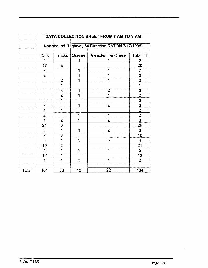
DATA COLLECTION SHEET FROM 7 AM TO 8 AM
Northbound (Highway 64 Direction RATON 7/17/1998) I ,..._
Trucks Queues Vehicles per Queue Total DT 2 1 1 2 17 3 20 2 1 1 2 2 1 1 2
2 1 1 2 1 1 3 1 2 3 2 1 1 2
2 1 3 3 1 2 3 1 1 2 2 1 1 2 1 2 1 2 3
21 8 £'tJ
2 1 1 2 h 7 3 3 1 1 3 4 19 2 21 4 1 1 4 5 12 1 13
I 1 1 1 1 2
Total: 101 33 13 22 134
Project 7-3951 Page F- 93

DATA COLLECTION SHEET FROM 8 AM TO 9 AM I
Northbound (Highway 64 Direction RATON 7/17/1998) i i
I Cars Trucks Queues Vehicles per Queue Total DT i 9 1 10
2 1 1 2 3 3 3 1 1 1 1 2 3 3
2 1 1 2 14 3 17 1 3 1 3 4 2 2 1 1 1 1 2
2 1 1 2 5 2 7 2 1 1 2 3
I 2 1 1 2 3 5 5
I 2 1 1 2 3 2 2 4 i
2 1 1 2 3 I I 1 1 1 1 2
2 1 1 2 3 9 9 1 1 1 1 2 !
7 7 2 1 1 2 3 1 1 1 1 2 3 3 1 1 1 1 2 1 2 3 1 1 1 1 2
11 1 12 2 2 1 3 4 5 5 2 1 1 2 3 10 1 11
i 3 1 1 3 4 I 14 14
2 1 1 2 3 2 1 1 2
Project 7-3951 Page F- 94
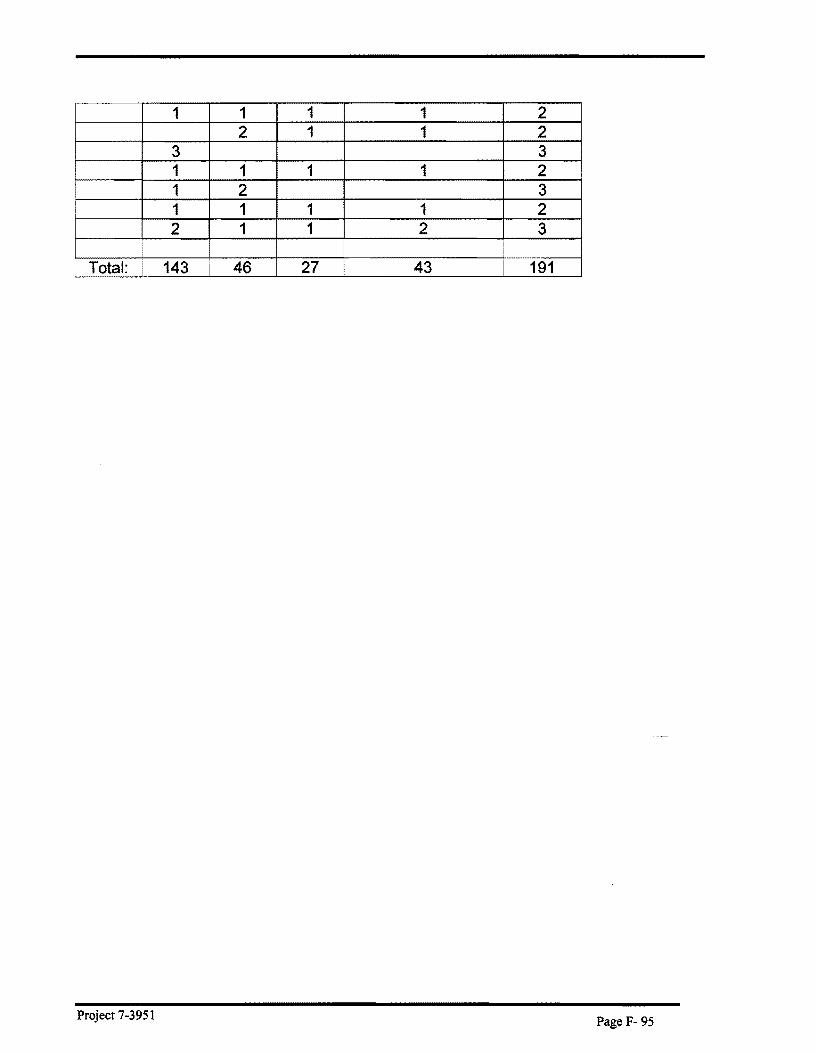
1 1 1 1 2 2 1 1 2
3 3 1 1 1 1 2 1 2 3 1 1 1 1 2 2 1 1 2 3
Total: 143 46 27 43 191
Project 7-3951 Page F- 95
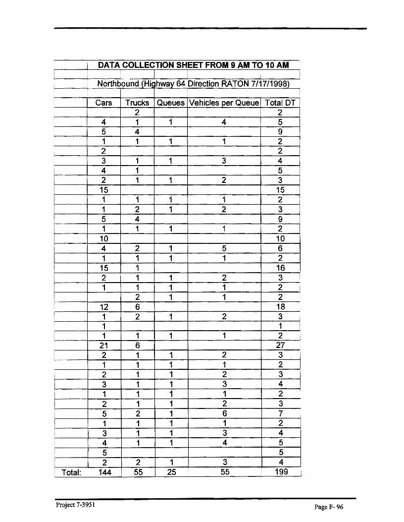
DATA COLLECTION SHEET FROM 9 AM TO 10 AM I i
Northbound (Hi~ hway 64 Direction RATON 7/17/1998)
Cars Trucks Queues Vehicles per Queue Total DT · 2 2
4 1 1 4 5 5 4 9 1 1 1 1 2 ...
2 2 3 1 1 3 4 I
4 1 5 I 2 1 1 2 3 i
15 15 I
i 1 1 1 1 2 i I 1 2 1 2 3 I 5 4 9 : 1 1 1 1 2 • 10 10 I 4 2 1 5 6
1 1 1 1 2 I 15 1 16
2 1 1 2 3 1 1 1 1 2
2 1 1 2 I
12 6 18 I
1 2 1 2 3 1 1 1 1 1 1 2
• 21 6 27 I
2 1 1 2 3 I 1 1 1 1 2 I
I 2 1 1 2 3 3 1 1 3 4 I
1 1 1 1 2 2 1 1 2 3
I 5 2 1 6 7 I 1 1 1 1 2 i 3 1 1 3 4 I 4 1 1 4 5 i 5 5
2 2 1 3 4 Total: 144 55 25 55 199
Project 7·3951 Page f. 96

Project 7-3951 Page F- 97

DATA COLLEC"riON SHEET FROM 10 AM TO 11 AM I
.
Northbound (Hi~hway 64 Direction RATON 7/17/1998} i I
Cars Trucks Queues Vehicles per Queue Total DT 1
10 3 13 I I 1 1 1 1 2 I
1 1 1 1 2 I 3 1 1 3 4 1 1 1 1 2 4 2 1 5 6
I 4 1 1 4 5 I 1 1 1 1 2 I 7 7 I 3 1 1 3 4 . 1 1 1 1 2
10 1 11 i 2 1 1 2 3
2 1 1 2 3 3 1 1 3 4
I 15 3 18 I 1 2 1 2 3
8 2 1 9 10 2 1 1 2 3 16 9 25 1 1 1 1 2 1 1 1 1 2
I 2 1 1 2 6 1 1 6 7 2 2 1 3 4 2 1 1 2 3 2 1 1 2 3 4 1 1 4 5 3 1 1 3 4 1 1 1 1 2 1 1 1 1 2 3 1 1 3 4 1 1 1 1 2 2 1 1 2 3 1 1 1 1 2 3 1 1 3 4 3 1 1 3 4 1 1 1 1 2
Project 7-3951 Page F- 98

1 2 1 2 3 I
t-+-t 1 1 5 7 2 16
1 1 1 1 2 1 1 1 1 2 1 1 1 1 2 1 1 1 1 2 1 1 1 1 2 1 1 1 1 2 9 3 1 11 12 7 1 8 2 1 1 2 3 3 1 1 3 4 1 1 1 1 2 1 1 1 1 2
•
Total: 182 73 46 110 255
Project 7-3951 Page F- 99
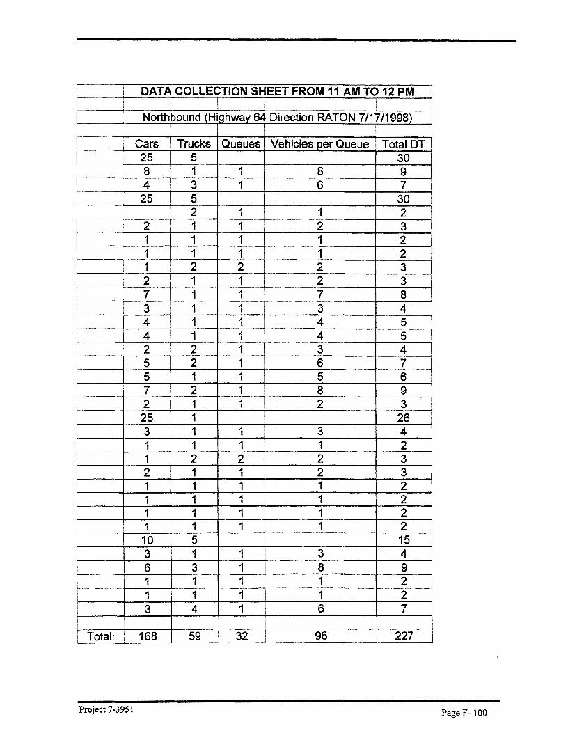
! i DATA COLLECTION SHEET FROM 11 AM TO 12 PM ! I I I
Northbound (Highway 64 Direction RATON 7/17/1998) i
i
I Cars Trucks Queues Vehicles per Queue Total DT 25 5 30
! 8 1 1 8 9 I 4 3 1 6 7 I I
25 5 30 !
i 2 1 1 2 ' I 2 1 1 2 3 i
1 1 1 1 2 J 1 1 1 1 2
I 1 2 2 2 3 2 1 1 2 3 7 1 1 7 8 3 1 1 3 4 i
I 4 1 1 4 5 4 1 1 4 5 2 2 1 3 4 5 2 1 6 7
I 5 1 1 5 6 7 2 1 8 9 2 1 1 2 3 25 1 26 J 3 1 1 3 4 1 1 1 1 2
i 1 2 2 2 3 i
2 1 1 2 3 J 1 1 1 1 2 1 1 1 1 2 J 1 1 1 1 2 i
I 1 1 1 1 2 i 10 5 15 I
3 1 1 3 4 I 6 3 1 8 9
1 1 1 1 2 I 1 1 1 1 2 i 3 4 1 6 7 i
Total: 168 59 32 96 227
Project 7-3951 Page F- 100

DATA COLLECTION SHEET FROM 12 AM TO 1 PM 1 I I I
Northbound (Highway 64 Direction RATON 711711998)
Cars Trucks Queues Vehicles per Queue Total DT 1 1 1 1 2
23 2 25 1 1 1 1 2 2 1 1 2 3
I 1 1 1 1 2 1 1 1 1 2
I 25 1 26 1 3 1 3 4 8 3 1 10 11 1 1 1 1 2
! 16 4 20 2 1 1 2 3 1 1 1 1 2
20 8 28 5 1 1 5 6 1 1 1 1 2 1 1 1 1 2 1 1 1 1 2 1 1 1 1 2 I
2 1 1 2 3 20 3 23 2 1 1 2 3 1 1 1 1 2 1 1 1 1 2
15 2. 17 1 1 1 1 2 2 1 1 2 3 14 1 1 14 15
Total: 170 46 22 55 216
Project 7-3951 · Page F- 101

DATA COLLECTION SHEET FROM 1 PM TO 2 PM I !
Northbound (Hinhway 64 Direction RATON 7/17/1998] J !
I Cars Trucks Queues Vehicles per Queue Total DT 20 11 31
i 1 2 1 2 3 1 1 1 1 2 1 1 1 1 2
r 1 1 1 1 2 2 2 1 3 4
I 1 1 1 1 2 I 1 1 1 1 2
4 1 1 4 5 21 1 22 I
I 1 1 1 1 2 1 1 1 1 2 3 2 1 3 5 4 1 1 4 5 1 1 1 1 2 2 1 1 2 3 30 30 1 1 1 1 2 I
1 1 1 1 2 2 1 1 2 3 5 1 1 5 6 1 1 1 1 2 1 1 1 1 2 2 1 1 2 3 25 7 32
I 1 1 1 1 2 I
4 1 1 4 5 i 3 2 1 4 5 I
1 1 1 1 2 !
3 2 1 4 5 2 1 1 2 3 1 1 1 1 2 2 1 1 2 3 1 1 1 1 2 3 1 1 3 4
Total: 154 55 31 62 209
Project 7-3951 Page F- 102

DATA COLLECTION SHEET FROM 2 PM TO 3 PM I
I !
Northbound (Highway 64 Direction RATON 7/17/1998)
Cars Trucks Queues Vehicles per Queue Total DT 25 I 1 26 1 1 1 1 2 2 2 1 3 4 1 1 1 1 2 5 1 1 5 6 1 1 1 1 2 5 1 1 5 6
25 2 27 2 1 1 2 3 1 1 1 1 2 3 1 1 3 4 4 1 1 4 5 1 1 1 1 2 1 1 1 1 2
! 6 1 1 6 7 1 1 1 1 2 2 1 1 2 3 2 1 1 2 3 25 25 3 1 1 3 4 2 1 1 2 3 1 1 1 1 2 1 1 1 1 2 1 1 1 1 2 1 1 1 1 I 2 2 3 1 4 5 2 I 1 1 2 3 1 1 1 1 2 1 2 1 2 3 6 1 1 6 7 1 1 1 1 2 5 5 3 1 1 3 4 1 1 1 1 2 1 1 1 1 2 1 1 1 1 2 3 1 1 3 4 1 1 1 1 2
Project 7-3951 Page F- 103

I 29 3 32 I 2 1 1 2 3 J
2 1 1 2 3 2 1 1 2 3 2 1 1 2 3 1 1 1 1 2 1 1 1 1 2 I
1 1 1 1 2 1 1 1 1 2 I
I 1 1 1 1 2 1 1 1 1 2 5 2 1 6 7
I
Total: 198 56 45 94 254
Project 7-3951 Page F-104

DATA COLLECTION SHEET FROM 3 PM TO 4 PM I I I
Northbound (Hi! hway 64 Direction RATON 7/17/1998)
Cars Trucks Queues Vehicles per Queue Total DT 25 25 1 1 1 1 2 1 1 1 1 2 1 1 1 1 2 5 1 1 5 6 1 1 1 1 2 1 1 1 1 2 2 1 1 2 3
~n H 36 1 2 3
1 1 1 1 2 1 1 1 1 2 4 2 1 5 6 3 1 1 3 4
i 25 15 1f-j I 3 1 1 3 • 2 1 1 2 3
1 1 1 1 2 1 j_2 1 2 3 1 1 1 1 2 2 1 1 2 3 4 2 1 5 6 3 1 1 3 4
30 3 33 2 1 1 2 3 2 1 1 2 3 4 1 3 4 1 1 1 1 2 3 1 1 3 4 ~ 1 1 2 3 10 10 4 1 1 4 5 12 1 1 12 13 2 1 1 2 3 3 1 1 3 4
Total: 30 77 251
Project 7-3951 PageF-105

! DATA COLLECTION SHEET FROM 4 PM TO 5 PM I J I Northbound (Highway 64 Direction RATON 7/17/1998) J
i
Cars Trucks Queues Vehicles per Queue Total DT I
30 3 33 I
I 1 1 1 1 2 2 1 1 2 3
I 2 1 1 2 3 I 3 1 1 3 4
1 1 1 1 2 1 1 1 1 2 3 1 1 3 4
I 30 2 32 2 1 1 2 3
2 1 1 2 1 1 1 1 2 4 1 1 4 5 1 3 1 3 4 5 3 1 7 8 3 1 1 3 4 2 1 1 2 3 I
1 1 1 1 2 2 1 1 2 3
i 8 3 1 10 11 2 1 1 2 3 3 1 1 3 4
I 2 1 1 2 3 I 27 1 28
3 1 1 3 4 2 1 1 2 3
I 2 1 1 2 3 I 2 1 1 2 3 I 1 1 1 1 2 I 2 2 1 3 4
1 1 1 1 2 I
1 1 1 1 2
I Total: 150 43 I 29 71 193
Project 7-3951 Page F- 106

DATA COLLECTION SHEET FROM 5 PM TO 6 PM
Northbound (Hi~ hway 64 Direction RATON 7/17/1998) I
Cars Trucks Queues Vehicles per Queue Total DT 1 1 1 1 2
25 2 27 3 1 1 3 4 3 1 1 3 4 4 1 1 4 5 2 1 1 2 3
•
2 1 1 2 2 1 1 2 3 1 1 1 1 2
25 4 29 1 1 1 1 2
• 1 1 1 1 2 1 2 1 2 3 1 1 I 1 2 1 1 I 1 2
25 2 27 3 1 1 3 4
I 1 1 1 1 2 1 1 1 1 2
25 1 26 2 1 1 2 3 1 1 1 1 2 1 1 1 1 2 2 1 1 2 3
•
Total: 132 31 20 34 163
Project 7-3951 Page F- 107

DATA COLLECTION SHEET FROM 6 AM TO 7 AM I I I I
Northbound (Highway 87 Direction Clayton 7/18/1998- Saturday)
i i
Cars Trucks Queues Vehicles per Queue Total DT 10 5 15 I
1 1 1 1 2 : 2 2 1 3 4
3 1 2 3 4 1 1 4 5 10 5 15
3 1 2 3 I 1 2 1 2 3
2 1 1 2 I I 10 5 15
2 1 1 2 3 4 1 1 4 5 10 1 11 1 1 1 1 2
I 9 9 10 5 15 2 1 1 2 3 1 1 1 1 2
I 4 1 1 4 5 I 2 1 1 2 3 I 10 13 23 J i 1 3 1 3 4 I
4 7 11 I
2 1 1 2 3 1 1 1 1 2
2 1 1 1 1 1 1 2
Total: 102 70 19 39 172
Project 7-3951 Page F- 108

DATA COLLECTION SHEET FROM 7 AM TO 8 AM
Northbound (Highway 87 Direction Clayton 7/18/1998 - Saturday)
I Cars Trucks Queues Vehicles per Queue Tota~ 10 5 15 10 5 15
I 1 1 1 1 2 1 1 1 1 2 3 1 1 3 4 i
1 1 1 1 2 10 5 15 1 1 1 1 2 1 5 6 1 2 1 2 3
10 5 15 10 1 11 2 1 1 2 3 10 5 15 2 1 1 2 3
I 1 1 1 1 2 2 1 1 2 3 2 1 1 2 3
I 10 5 t- ~5 1 2 1 2 i 2 2 1 3 4
1 1 1 1 2 2 2 1 3 4
I 5 1 1 5 6 i
1 1 1 1 2 10 5 15 I 1 1 1 1 2 I
2 1 1 2 3 2 1 1 2 3 10 1 11 1 1 1 1 2 I
10 10 15 15
i 2 3 1 4 5 2 1 1 2 3 1 1 1 1 2
i
Project 7-3951 Page F- 109

I Total: 156 72 24 46 228
Project 7-3951 Page F- 110

DATA COLLECTION SHEET FROM 8 AM TO 9 AM I I
Northbound (Highway 87 Direction Clayton 7/18/1998- Saturday}
Cars Trucks Queues Vehicles per Queue Total DT 15 5 20 15 5 20 2 1 1 2 3
• 1 1 1 1 2
I 1 1 1 1 2 3 1 1 3 4
•
15 5 20 I 4 1 1 4 5
I 1 1 1 1 2 15 5 20
I 1 1 1 1 2 10 3 13
I 3 1 3 4 ! 2 1 1 2
15 1 16 2 1 1 2 3
I 1 1 1 1 2 15 15 1 1 1 1 2
15 1 . 16 1 1 1 1 2 2 1 1 2 3 2 1 1 2 3 5 3 1 7 8 1 2 1 2 3 4 3 1 6 7 6 1 1 6 7 3 2 1 4 5 2 1 1 2 3 3 1 1 3 4 15 1 16
! 3 1 2 3 2 1 1 2
3 1 1 3 4 2 1 1 2 3 10 10 7 2 1 8 9
Project 7-3951 Page f. 111

2 1 1 2 3 I 10 2 12 r
1 1 1 1 2 1 1 1 1 2 6 6 6 1 1 6 7 1 1 1 1 2
I i l i ! Total: 1 226 73 32 73 299
Project 7-3951 Page F-112

DATA COLLECTION SHEET FROM 9 AM TO 10 AM
•
Northbound (Highway 87 Direction Clayton 7/18/1998- Saturday)
Cars Trucks Queues Vehicles per Queue Total DT 10 5 15
I 5 1 1 5 6 2 1 1 2 3 2 1 1 2 3 10 10 2 1 1 2 3 2 1 1 2 3
I 3 1 1 3 4 10 5 15 10 5 15 10 10 2 1 1 2 3 2 1 1 2 .;)
: 1 1 , 1 1 t={t= I 10 5 2 1 1 2 3 10 5 15 17 2 1 18 19 1 1 1 1 2 10 1 11 1 1 1 1 ?
•
3 1 1 3 4 I 1 1 1 1 2
10 1 11 4 1 1 4 5 2 4 1 5 6 1 2 1 2 3
10 10 1 1 1 1 2 1 2 1 2 3
10 1 11 10 1 11 1 1 1 1 2
10 10 4 1 1 4 t-~ 6 6 2 I 7 8
Project 7-3951 Page F- 113

! 10 5 15 I 3 2 1 4 5
10 5 15 1 1 1 1 2
I 10 10 10 10
I 3 1 1 3 4 2 1 1 2 3
I 1 2 1 2 3 1 1 1 1 2
I 1 1 1 1 2 10 10
I 4 4 1 7 8 1 1 1 1 2
I 10 10 5 4 1 8 9
I I 8 2 10 I 5 1 1 5 6 i 6 2 1 7 8 I 3 1 1 3 4 i
1 Total: 306 i 93 36 118 399
Project 7-3951 Page F- 114

DATA COLLECTION SHEET FROM 10 AM TO 11 AM !
! Northbound (Highway 87 Direction Clayton 7/18/1998 - Saturday)
Cars m Queues Vehicles per Queue Total DT 3 1 6 7 15 20 15 5 20 15 5 20 3 1 1 3 4 1 1 1 1 2 1 2 1 2 3 3 1 1 3 4
I 10 4 14 10 10 4 1 1 4 5
Hi 2 3 1 2 5 6
1 4 5 10 10 3 1 1 3 4 2 1 1 2 3 2 1 1 2 3 4 3 1 6 7 1 3 1 3 4 9 2 1 10 11 1 1 1 1 2 1 1 1 1 2 7 3 1 9 10
1 3 4 15 20 4 1 1 4 5 15 5 20 1 1 1 1 2
10 3 13 15 1 16 1 1 1 1 2 2 1 1 2 3 2 1 1 2 3 4 ±±C~ 6 7 6 6 7
Project 7-3951 Page F- 115
3 2 1 4 5 2 1 1 2 3 I
3 1 1 3 4 15 10 25 5 1 1 5 6 1 1 1 1 2
i 2 1 1 2 3 I 4 1 1 4 5 I 2 4 1 5 6
1 2 1 2 3 ~
1 1 1 1 2 i
1 2 1 2 3 6 2 1 7 8 I 1 1 1 1 2
Total: 256 104 40 132 360
Project 7-3951 Page F- 116

DATA COLLECTION SHEET FROM 11 AM TO 12 PM
Northbound (Highway 87 Direction Clayton 7/18/1998- Saturday)
Cars Trucks Queues Vehicles per Queue Total DT 10 5 15 1 1 1 1 2
10 5 15 2 1 1 2 3
2 1 1 2 2 1 1 2 3 10 3 13 3 1 1 3 4 4 1 1 4 5 3 1 1 3 4 10 1 1 10 11 10 10 2 1 1 2 3 2 1 1 2 3 1 2 1 2 3 2 1 1 2 3 7 7 3 1 1 3 4 5 1 1 5 6 2 1 1 2 3 10 10 2 1 1 2 3 10 5 15 2 1 1 2 3 10 5 15 4 1 1 4 5 2 4 1 5 6 1 2 1 2 3 1 1 1 1 2 1 2 1 2 3 6 2 1 7 8 15 15 15 1 16 1 1 1 1 2 2 1 1 2 3 2 1 1 2 3 3 1 1 3 4
Project 7-3951 Page F- 117
15 1 16 10 5 15 7 2 1 8 9 2 1 1 2 3 10 2 12 2 2 I 1 3 4 1 1 1 1 2 5 1 1 5 6 1 1 1 1 2
10 4 1 13 14 10 1 11 2 1 1 2 3 10 7 17 2 1 1 2 3 1 2 1 2 3 2 2 1 3 4 1 1 1 1 2
Total: 267 94 39 120 361
Project 7-3951 Page F- 118

DATA COLLECTION SHEET FROM 12 PM T
Northbound (Hiohwav 87 Direction Clavton 7/18/1998- S
Cars Trucks Queues Vehicles per Queue Total DT 30 8 I 38
I 7 1 1 7 8 35 5 40 2 1 1 2 3
1 1 3 4 1 1 3 4 2 1 11 12
30 5 35 1 1 1 2 1 1 1 2 1 1 1 1
~ 1 1 1 1 30 5 2 1 1 2 3 1 1 3 4
i 1 2 1 2 3 ! 1 1 1 1 2
6 1 1 6 (
1 1 1 1 2 2 2 1 3 4 5 6 1 10 11
0 1 1 2 3 1 1 8 9
1 1 1 1 2 I 1 1 1 1 2
1 1 1 1 2 I 2 1 2 3
3 I 1 1 3 4 7 1 1 7 8 6 1 5 6 2 1 1 2 3 3 2 1 4 r:
40 5
f$ 6 2 1 7 4 2 1 5 2 1 1 2 16 6 1 21 22
Project 7-3951 Page F- 119
I I 1 I 1 1 1 2 I i
i Total: I 279 I 77 33 130 356
Project 7~3951 Page F- 120

DATA COLLECTION SHEET FROM 1 PM TO 2 PM I I
Northbound I (Highway 87 Direction Clayton 7/18/1998 - Saturday)
I
Cars Trucks Queues Vehicles per Queue Total DT 25 5 30 8 1 1 8 9 4 I 3 1 6 7 25 I 5 30
2 1 1 2 25 5 30 7 1 1 7 8
2 1 1 2 4 5 1 8 9 3 1 1 3 4 2 4 1 4 5
25 30 8 4 1 11 12 10 1 1 10 11 1 1 1 1 2
25 5 30 2 1 1 2 3
25 1 26 3 3 1 5 6 10 10 3 1 1 3 4 6 3 1 8 9 1 1 1 1 2 1 1 1 1 2 3 4 1 6 7
Total: 226 64 18 86 290
Project 7-3951 Page F- 121
DATA COLLECTION SHEET FROM 2 PM TO 3 PM
Northbound (Highway 87 Direction Clayton 7/18/1998- Saturday)
Cars Trucks Queues Vehicles per Queue Total DT 25 5 30 4 1 1 4 5 3 1 1 3 4 2 1 1 2 3 3 2 1 4 5 4 1 1 4 5 11 2 1 12 13 10 2 1 11 12 25 5 30 7 1 1 7 f= 8 1 1 8 2 2 1 3 4j
25 5 30 2 1 1 2 3 1 1 1 1 2
25 5 30 3 1 1 3 4
26 5 31 4 1 1 4 5 4 1 1 4 5
• 4 1 1 4 5 2 2 1 3 4 5 2 1 6 7 5 1 1 5 6 7 2 1 8 9 25 3 28 3 2 1 4 5 2 1 1 2 3 2 2 1 3 4 5 2 1 6 7 13 5 1 17 18 5 4 1 8 9 8 1 1 8 9
Total: 280 72 27 146 352
Project 7-3951 Page F- 122

DATA COLLECTION SHEET FROM 3 PM TO 4 PM
Northbound {Highway 87 Direction Clayton 7/18/1998 - Saturday)
Cars Trucks I Queues I Vehicles ~er Queue Total DT 1 3 1 2 1 2 3
25 5 30 4 2 1 5 6 3 2 1 4 5
25 5 30 7 2 1 8 9 5 3 1 7 8
25 5 30 6 1 1 6 7 5 1 1 5 6 2 1 1 2 3 1 1 1 1 2 1 2 1 2 3
25 5 30 1 1 1 1 2 5 1 1 5 6
25 25 4 3 1 6 7 10 1 I 10 11 4 1 4 5 7 2 1 8 9 2 1 1 2 3 3 1 1 3 4 1 1 1 1 2
25 5 30 3 1 1 3 4 2 2 1 3 4 13 3 16 2 1 1 2 3
•
6 1 1 6 7 15 1 1 15 16
i
Total: 264 65 25 113 329
Project 7-3951 Page F- 123

DATA COLLECTION SHEET FROM 4 PM TO 5 PM
Northbound (Highway 87 Direction Clayton 7/18/1998- Saturday) i
I
Cars Trucks Queues Vehicles per Queue Total DT 20 5 25 2 1 1 2 3 20 5 25 2 1 1 2 3 3 1 1 3 4 5 4 1 8 9 1 1 1 1 2 2 1 1 2 3
20 5 25 i 1 1 1 1 2
20 4 1 23 24 20 5 25 4 2 1 5 6 5 1 1 5 6
20 1 21 3 1 1 3 4 !
2 2 1 3 4 1 1 1 1 2
11 2 1 12 13 6 1 1 6 7
'
20 20 2 1 1 2 I
I 8 1 1 8 9 4 4
1 Total: 200 48 17 86 248
Project 7-3951 Page F-124

DATA COLLECTION SHEET FROM 5 PM TO 6 PM
Northbound (Highway 87 Direction Clayton 7/18/1998- Saturday)
Cars Trucks Queues Vehicles per Queue Total DT 10 4 1 13 14 20 5 25 3 1 1 3 4 6 1 1 6 7
20 5 25 2 1 1 2
20 5 25 1 1 1 1 2 4 1 1 4 5 5 3 1 7 8 4 3 1 6 7 4 1 1 4 5 20 1 21 2 1 1 2 3 17 17 1 1 1 1 2
Total: 137 35 11 48 172
Project 7-3951 Page F- 125
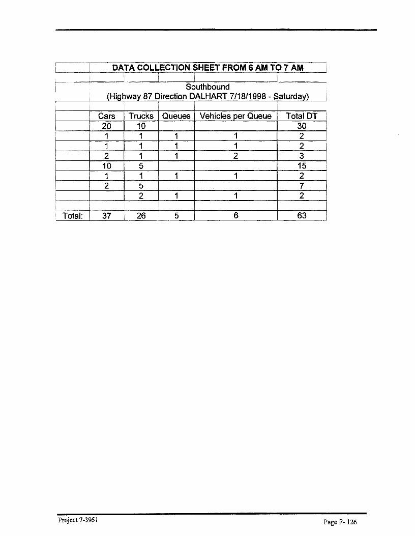
DATA COLLECTION SHEET FROM 6 AM TO 7 AM I
i
I Southbound I I (Highway 87 Direction DALHART 7/18/1998 - Saturday) !
Cars Trucks Queues Vehicles per Queue Total DT 20 10 30 1 1 1 1 2 1 1 1 1 2 2 1 1 2 3 10 5 15 1 1 1 1 2 2 5 7
2 1 1 2
Total: 37 I 26 5 6 63
Project 7-3951 Page F- 126

DATA COLLECTION SHEET FROM 7 AM TO 8 AM
•
I . Southbound (Highway 87 Direction DALHART 7/18/1998- Saturday)
Cars Trucks Queues Vehicles per Queue Total DT 30 15 45
2 1 1 2 1 1 1 1 2
I 1 1 1 1 2 i 1 2 1 2 ,)
1 1 1 1 2 7 2 9 1 2 1 2 3 3 4 1 6 7
Total: 45 30 7 14 I 75
Project 7-3951 Page F- 127

DATA COLLECTION SHEET FROM 8 AM TO 9 AM
I (Highway 87 Direction DALHART 7/18/1998 - Saturday) I I Cars Trucks Queues Vehicles _per Queue Total DT ! 30 5 35 I 2 1 1 2 3 I 1 1 1 1 2 I 30 5 35 I 5 2 1 6 7 ' I 1 1 1 1 2 I 2 1 1 2 3 i 1 1 1 1 2
1 1 1 1 2 I
I 1 1 1 1 2 I ! 14 2 16 I
I 2 3 1 4 5
I Total: 90 24 9 19 I 114
Project 7-3951 Page F-128

DATA COLLECTION SHEET FROM 9 AM TO 10 AM
s thb d I
ou oun i (Highway 87 Direction DALHART 7/18/1998 - Saturday)
I I I
Cars I Trucks Queues Vehicles per Queue Total DT 1
! 30 1 31 I 5 2 1 6 7
2 1 1 2 3 2 1 1 2 3
I 2 1 1 2 3 I 5 1 1 5 ·6
2 1 1 2 3 ! 4 1 1 4 5 I 1 1 1 1 2
25 3 28 6 3 1 8 9 4 2 1 5 6 1 3 1 3 4 1 1 1 1 2 2 2 1 3 4
I 1 1 1 1 2 7 1 1 7 8 3 1 1 3 4
I 1 1 1 1 2 9 1 10 7 1 1 7 8 5 1 1 5 6
I
Total: 125 I 31 19 68 156
Project 7-3951 Page F- 129

DATA COLLECTION SHEET FROM 10 AM TO 11 AM ! i I I
I Southbound I (Highway 87 Direction DALHART 7/18/1998- Saturday) I
Cars Trucks Queues Vehicles per Queue Total DT 1 1 1 1 2 :
i
25 3 28 3 1 1 3 4 3 1 1 3 4
i 1 1 1 1 2 I 6 3 1 8 9 ! 3 1 1 3 4
1 1 1 1 2 I 6 1 1 6 7 ! 15 1 16
2 2 1 3 4 I 2 3 1 4 5
2 1 1 2 3 i 3 1 1 3 4 I 15 5 20 1 4 1 1 4 5 i
! 1 1 1 1 2 I
I 15 5 20 1 1 1 1 2
10 3 13 I 1 1 1 1 2 ! 6 1 1 6 7 I 1 1 1 1 2 I 2 1 1 2 3 i 2 1 1 2 3
I 5 3 1 7 8 I 3 2 1 4 5 I 4 1 3 4
I I
I Total: 143 47 I 23 70 190
Project 7-3951 Page F- 130

DATA COLLECTION SHEET FROM 11 AM TO 12 PM
Southbound I (Highway 87 Direction DALHART 7/18/1998 - Saturday)
Cars Trucks Queues Vehicles per Queue Total DT 25 4 29 2 1 1 2 3 3 1 1 3 4 3 1 1 3 4 6 1 1 6 7 2 1 1 2 3 5 1 1 5 6 I
4 1 1 4 5 5 5 6 1 1 6 7 3 3 3 1 1 3 4 12 2 14 5 1 1 5 6 3 1 1 3 4 6 1 1 6 7 3 1 1 3 4 2 3 1 4 5 25 5 30 1 1 1 1 2 4 1 1 4 5 22 22 8 3 1 10 11 10 1 1 10 11
I 1 1 1 1 2 I 25 1 26
3 2 1 4 5 3 1 1 3 4 6 3 1 8 9 1 1 1 1 2
! 1 1 1 1 2 3 2 1 4 5 2
1 2 I 1 3 4 !
Total: 213 I 47 26 105 260
Project 7-3951 Page F- 131

I DATA COLLECTION SHEET FROM 12 PM TO 1 PM I I I J I Southbound i I (Highway 87 Direction DALHART 7/18/1998 - Saturday) I I
Cars Trucks Queues Vehicles _per Queue Total DT i 30 5 35 I 2 2 1 3 4
2 1 1 2 3 i 9 3 1 11 12 I 3 1 1 3 4
4 1 1 4 5 I i 6 1 5 6 !
1 1 1 1 2 I
2 1 1 2 3 I 4 1 3 4 J
8 1 1 8 9 i
7 3 1 9 10 1 1 1 1 2 1 1 1 1 2 7 1 1 7 8 25 2 27 1 1 1 1 2 i
1 1 1 1 2 I 14 1 1 14 15 I
1 1 1 1 2 4 3 1 6 7 I
i 5 2 1 6 7 25 1 26 7 1 1 7 8
! 2 2 1 3 4 4 1 1 4 5 2 1 1 2 3 2 1 1 2 3 2 1 1 2 3 6 1 1 6 7 3 1 1 3 4
25 25 I 1 2 1 2 3
1 2 1 2 3 i 2 1 1 2 3 I 10 8 1 17 18
2 1 1 2 3
Project 7-3951 Page F- 132

3 3
Total: 231 i 61 33 143 292
Project 7-3951 Page F- 133

DATA COLLECTION SHEET FROM 1 PM TO 2 PM i !
Southbound (Highway 87 Direction DALHART 7/18/1998- Saturday)
i
Cars Trucks Queues Vehicles per Queue Total DT i 25 1 26 I
i 13 1 1 13 14 I 1 1 1 1 2 ! 4 1 1 4 5
2 1 1 2 3 25 25 4 1 1 4 5
I 1 1 1 1 2 10 1 1 10 11
i 3 1 1 3 4 25 1 26 1 1 1 1 2 1 1 1 1 2
i 1 1 1 1 2 I 2 1 1 2 3 I 3 1 1 3 4 i
! 25 25 i 1 1 1 1 2 I 3 2 1 4 5
I 4 3 1 6 7 2 1 1 2 3
I 4 1 3 4 1 2 1 2 3
! 7 1 1 7 8 6 1 5 6 i
4 2 1 5 6 2 4 1 5 6 25 3 28
I 3 1 1 3 4 3 1 1 3 4
! 2 1 1 2 3 12 1 13
: 1 1 1 1 2
I 4 2 1 5 6 2 1 1 2 3
i 4 1 1 4 5 i 1 1 1 1 2
Project 7-3951 Page F-134
: Total: 237 44 31 107 281
Project 7-3951 Page F- 135

I DATA COLLECTION SHEET FROM 2 PM TO 3 PM I
I
! I Southbound
I I
(Highway 87 Direction DALHART 7/18/1998- Saturday) I
Cars Trucks Queues Vehicles per Queue Total DT I
25 2 27 I 2 1 1 2 3 I 2 2 1 3 4 J I 1 1 1 1 2 I I 5 1 1 5 6 I I 3 3 1 5 6 I
: 2 1 1 2 3 I 25 2 27
4 1 1 4 5 2 1 1 2 3 4 4 1 7 8 22 22 2 1 1 2 3 25 1 1 25 26 2 2 1 3 4 1 1 1 1 2 i
! 5 1 1 5 6 1 1 1 1 2 i
25 25 I
I 3 1 1 3 4 3 1 1 3 4
I 4 1 1 4 5 3 1 1 3 4 5 2 1 6 7 6 1 1 6 7 5 2 1 6 7
25 4 29 i 7 1 1 7 8 I I 3 1 1 3 4 J
17 1 18 I
3 2 1 4 5 1 1 1 1 2 4 2 1 5 6
I 5 1 1 5 6
Total: 252 i 48 28 I 124 300
Project 7-3951 Page F- 136

DATA COLLECTION SHEET FROM 3 PM TO 4 PM
Southbound I i (Highway 87 Direction DALHART 7/18/1998- Saturday)
! Cars Trucks Queues Vehicles per Queue Total DT 25 25 4 1 1 4 5 4 1 1 4 5 1 2 1 2 3
25 4 29 i 2 1 1 2 3 I 2 1 1 2 3
1 1 1 1 2 I 2 1 1 2 3
3 1 1 3 4 I
5 3 1 7 8 3 1 1 3 4
25 2 27 5 4 1 8 9 1 2 1 2 3 2 1 1 2 3 3 3 1 5 6 4 2 1 5 6 I
4 1 1 4 5 25 2 27 9 1 1 9 10
25 25 3 2 1 4 5 1 1 1 1 2 4 1 1 4 5 25 3 28 3 1 1 3 4 2 1 1 2 3 I 3 1 1 3 4
I 5 1 4 5 i 22 22
1 1 1 1 2 I I i
1 Total: 249 46 25 87 295 I
Project 7-3951 Page F- 137

I I (Highway 87 Direction DALHART 7/18/1998 - Saturday) i
I I
i Cars Trucks Queues Vehicles per Queue Total DT I 25 4 29 i 2 1 1 2 3 I 2 1 1 2 3 i
i 10 2 1 11 12 i
I 25 5 30 i 2 1 1 2 3 I 1 1 1 1 2
19 6 1 24 25 I 11 2 1 12 13 i 25 5 30 I 7 1 1 7 8
3 1 1 3 4 I 1 1 1 1 2
5 3 1 7 8 I 25 2 27
3 1 1 3 4 1 1 1 1 2 3 1 1 3 4
25 4 29 1 1 1 1 2 1 1 1 1 2
I 1 1 1 1 2 I 3 1 1 3 4 I 5 5 I 12 1 1 12 13 ! i I Total: 218 48 19 97 266
Project 7-3951 Page F-138

DATA COLLECTION SHEET FROM 5 PM TO 6 PM
i (Highway 87 Direction DALHART 7/18/1998- Saturday) 1
i
Cars Trucks Queues Vehicles per Queue Total DT 25 2 27 2 1 1 2 3
! 1 2 1 2 3 1 1 1 1 2
i 25 2 27 I 3 3 1 5 6 I
I 2 2 1 3 4 3 1 1 3 4 i
I 1 1 1 1 2 25 1 26 8 4 12 1 1 1 1 2 5 3 1 7 8
25 2 27 25 1 26 3 1 1 3 4
I 11 2 1 12 13 I 3 1 2 3
5 1 1 5 6 I 25 2 27
1 2 1 2 3 i 1 2 1 2 3
6 3 1 8 9 1 1
I i i
Total: 1 208 40 16 59 248
Project 7-3951 Page F- 139

REFERENCES L AASHTO, (1990), 'A Policy on Geometric Design of Highways and Streets, American
Association of State Highway and Transportation Officials, Washington D.C.
2. AASHTO, (1994), 'Passing site distance for Two-lane Highways', A Policy on Geometric Design of Highways and Streets, Washington D.C. pp 128-134.
3. Central North American Trade Corridor Association, (1997). "High Priority Trade Corridor, U.S. Highways 83 and 52," CNTCA, Minot, North Dakota.
4. Eyler, Dennis R. and Poletz, Alex, (1996). 'The Super Two', Semisequicentennial Transportation Conference Proceedings, pp 38-39.
5. Frost, Dr. -Ing. Uwe and Morrall, John (1995), 'A Comparison and Evaluation of the Geometric Design Practices with Passing Lanes, Wide-Paved Shoulders and Extra-Wide Two-Lane Highways in Canada and Germany', International Symposium on Highway Geometric Design Practices, Transportation Research Board, Boston, Massachusetts, USA, pp 1-12.
6. Garber, J. Nicholas and. Hoel, A. Lester, (1997) ,'Introduction to Queuing Theory', Traffic And Highway Engineering, Second Edition, Department of Civil Engineering, University ofVirginia, pp 208-218.
7. Garber, J.N., Hoel, A.L. (1997), 'Traffic and Highway Engineering-Second Edition', Department of Civil Engineering, University of Virginia
8. Gattis, J.L., Alguire, Mary, S. Townsend, Kristy and Rao Shreenath, (1997), 'Rural two-lane Passing Headways and Platooning', Transportation Research Record, 1579, pp 27-34.
9. Gransberg, D.D., S.P. Senadheera, E. Silay, and I.Karaca (1998). "Economic Evaluation Of Super Two Highway Design Geometry", Texas Department of Transportation Research Report TX-98-7-3951-2R, pp. 2-36.
10. Grumet, W. Gerald, (1989), 'Emotional Aspects Of Motoring', Psychoanalytic Review, pp 19-34.
11. Harwood, D.W. and Hoban, C. J. (1987), 'Low cost methods for improving traffic operations on two lane roads: Informational Guide'. Report FHWA-IP-87-2. FHWA, U.S. Department of Transportation.
12. Guell, D.L. and Virkler, M.R. (1998), 'Capacity Analysis of Two-lane Highways. Transportation Research Record 1194 (TRB), National Research Council, Washington, D.C. pp 199-203.
13. Heimbach, C.L.,W.W. Hunter, and G.C. Chao (1974). "Paved Highway Shoulder Accident Experience," J. of Transportation Engr, ASCE 100 (TE4), New, York, NY, 889-907.
Project 7-3951 Page Bib-1

14. Highway Research Board, Special Report, (1987), 'Two-Lane Highways', Highway Capacity Manual, National Research Council, pp 299-317.
15. Hoban, C.J. (1983), 'Towards a Review of The Concept of Level of Service for Two-lane Roads.', Australian Road Research, Vol. 13, No.3, pp 216-218.
16. Khasnabis, S. and C.L. Heimbach, (1980). "Headway Distribution Models for Two-Lane Rural Highways," Transportation Research Record 772, TRB, National Research Council, Washington, D.C., 44-51.
17. McDonald, M., M.a. Brackstone, and D. Jeffery (1994). "Simulation of Lane Usage Characterisitics on Three Lane Motorways," Proceedings, 27th International Symposium on Automotive Technology and Automation, Aachen, Germany, 365-372.
18. Mendoza, Alberto and Mayoral, Emilio, (1995),'Design Guidelines for Truck Lanes on Mexican Two-Lane Roads', Transportation Research Record 1523, pp91-98.
19. Messer, C.J. and Morral, J.F. (1983), 'Two-lane, Two-way Rural Highway Capacity.', Final Report, NCHRP Project 3-28A. Texas Transportation Institute, (TTl), College Station.
20. Morrall, John F. and Werner, Al, (1992), 'Measuring Level of Service of Two-Lane Highways by Overtakings', Transportation Research Record 1287, pp 62-69.
21. Newnan, D.G., (1996). Engineering Economic Analysis, 6th Edition, Engineering Press, San Jose, California.
22. Operation and Procedures Manual 2-94 (Part IV). (1994). Design Division. Texas Department of Transportation (TX DOT)
23. Oppy, E.T., (1992). "Life Cycle of Lesser Roads: Balancing Motorists: Wishes and Managers Budgets," Proceedings, Seventh Conference of the Road Engineering Association of Asia and Australia, Singapore, Vol 2, 786-794.
24. Papacostas, C.S. and Prevedouros, P.D, (1993),'Probability, Queuing and Simulation Models', Transportation Engineering and Planning, Second Edition, University of Hawaii at Manoa, pp 599-632.
25. Pitstic, Mark E., (1991) 'Measuring delay and Simulating Performance at Isolated Signalized Intersections using cumulative Curves', Transportation Research Record 1287, pp 34-41.
26. Sandahl, J.E., (1996), "Design Guidelines for Super Two, a High Volume Two-Lane Highway," Technical Memorandum No. 96-ES, Minnesota Department of Transportation, St. Paul, Minnesota.
27. Special Report 209: Highway Capacity Manual (1994), 3rd Ed. TRB, National Research Council, Washington, D.C.
Project 7-3951 Page Bib-2

28. Steve, G. Gabany, Portia Plummer, and Pat Grigg, (1997), 'Why drivers speed: The speeding perception', Journal of Safety Research, VoL 28, No. 1, pp 28-36.
29. 'Technical Memorandum No. 96- -ES-, (November 7, 1996), Engineering Services Division, Minnesota Department of Transportation (Minnesota DOT).
30. Xing, H.(1989). Suggestions on the Improvement ofTwo-Lane Highways for Mixed Traffic, Ministry of Communications, China Highway Research Institute, Beijing, China, 20-28.
Project 7-3951 Page Bib-3