two dimensional graphics transformations geometric ... · two dimensional graphics transformations...

Sri Vidya College of Engineering & Technology, Virudhunagar Course Material (Lecture Notes)

CS6504 & Computer Graphics Unit I

TWO DIMENSIONAL GRAPHICS TRANSFORMATIONS

Geometric Transformations

Changes in size, shape are accomplished with geometric transformation. It alter the

coordinate descriptions of object.

The basic transformations are Translation, Roatation, Scaling. Other transformations are

Reflection and shear.Basic transformations used to reposition and resize the two dimentional

objects.

Two Dimensional Transformations

Translation

A Translation is applied to an object by repositioning it along a straight line path from one

co-ordinate location to another. We translate a two dimensional point by adding translation

distances tx and ty to the original position (x,y) to move the point to a new location (x’,y’)

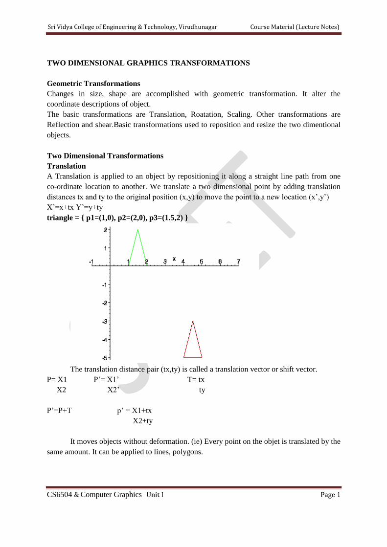
X’=x+tx Y’=y+ty

triangle = { p1=(1,0), p2=(2,0), p3=(1.5,2) }

The translation distance pair (tx,ty) is called a translation vector or shift vector.

P= X1 P’= X1’ T= tx

X2 X2’ ty

P’=P+T p’ = X1+tx

X2+ty

It moves objects without deformation. (ie) Every point on the objet is translated by the

same amount. It can be applied to lines, polygons.



Rotation

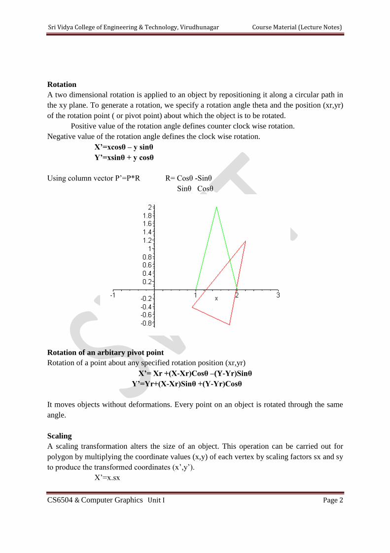
A two dimensional rotation is applied to an object by repositioning it along a circular path in

the xy plane. To generate a rotation, we specify a rotation angle theta and the position (xr,yr)

of the rotation point ( or pivot point) about which the object is to be rotated.

Positive value of the rotation angle defines counter clock wise rotation.

Negative value of the rotation angle defines the clock wise rotation.

X’=xcosθ – y sinθ

Y’=xsinθ + y cosθ

Using column vector P’=P*R R= Cosθ -Sinθ

Sinθ Cosθ

Rotation of an arbitary pivot point

Rotation of a point about any specified rotation position (xr,yr)

X’= Xr +(X-Xr)Cosθ –(Y-Yr)Sinθ

Y’=Yr+(X-Xr)Sinθ +(Y-Yr)Cosθ

It moves objects without deformations. Every point on an object is rotated through the same

angle.

Scaling

A scaling transformation alters the size of an object. This operation can be carried out for

polygon by multiplying the coordinate values (x,y) of each vertex by scaling factors sx and sy

to produce the transformed coordinates (x’,y’).

X’=x.sx



Y’=y.sy

P= X1 P’= X1’ S= sx 0

X2 X2’ 0 sy

P’=P*S

If sx=sy , then it produces the uniform scaling

Sx<> sy , different scaling.

If sx,sy<0, then it produces the reduced object size

If sx,sy > 0, then it produces the enlarged size objects.

By choosing the position called fixed point, we can control the location of the scaled

object. This point is remain unchanged after the scaling transformation.

X’= Xf +(X-Xf)sx => X’= X.sx +(Xf(1-sx))

Y’=Yf+(Y-Yf)sy => Y’= Y.sy +Yf(1-sy)

Matrix representations and homogeneous coordinates

Graphics applications involves sequences of geometric transformations. The basic

transformations expressed in terms of

P’=M1 *P +M2

P, P’ --> Column vectors.

M1 --> 2 x 2 array containing multiplicative factors

M2 --> 2 Element column matrix containing translation terms

For translation --> M1 is the identity matrix

For rotation or scaling -->M2 contains transnational terms associated with the pivot

point or scaling fixed point.



For coordinate positions are scaled, then rotated then translated, these steps are combined

together into one step, final coordinate positions are obtained directly from the initial

coordinate values.

To do this expand the 2 x 2 matrix into 3 x 3 matrix.

To express 2 dimensional transformation as a multiplication, we represent each cartesion

coordinate position (x,y) with the homogeneous co ordinate triple (Xh,Yh, h) where

X= xh/h, Y=Yh/h

So we can write (h.x, h.y,h), set h=1. Each two dimensional position is represented

with homogeneous coordinates(x,y,1). Coordinates are represented with three element

column vector. Transformation operations are written as 3 by 3 matrices.

For translation

X’ 1 0 tx X

Y’ 0 1 ty Y

1 0 0 1 1

P’=T(tx,ty)*P

Inverse of the translation matrix is obtained by replacing tx, ty by –tx, -ty

Similarly rotation about the origin

X’ Cosθ -Sinθ 0 X

Y’ Sinθ Cosθ 0 Y

1 0 0 1 1

P’= R(θ)*P

We get the inverse rotation matrix when θ is replaced with (-θ)

Similarly scaling about the origin

X’ Sx 0 0 X

Y’ 0 Sy 0 Y

1 0 0 1 1

P’= S(sx,sy)*P

Composite transformations

- sequence of transformations is called as composite transformation. It is obtained by forming

products of transformation matrices is referred as a concatenation (or) composition of

matrices.

Tranlation : -

Two successive translations

1 0 tx 1 0 tx 1 0 tx1+tx2

0 1 ty 0 1 ty 0 1 ty1+ty2



0 0 1 0 0 1 0 0 1

T(tx1,ty1) + T(tx2,ty2) = T(tx1+tx2, ty1+ty2)

Two successive translations are additive.

Rotation

Two successive rotations are additive.

R(θ1)* R(θ2)= R(θ1+ θ2)

P’=P. R(θ1+ θ2)

Scaling

Sx1 0 0 Sx2 0 0 Sx1.x2 0 0

0 Sy1 0 0 Sy2 0 0 Sy1.y2 0

0 0 1 0 0 1 0 0 1

S(x1,y1).S(x2,y2) = S(sx1.sx2 , sy1.sy2)

1. the order we perform multiple transforms can matter

eg. translate + scale can differ from scale + translate

eg. rotate + translate can differ from translate + rotate

eg. rotate + scale can differ from scale + rotate (when scale_x differs from scale_y)

2. When does M1 + M2 = M2 + M1?

M1 M2

translate translate

scale scale

rotate rotate

scale (sx = sy) rotate

General pivot point rotation

Rotation about any selected pivot point (xr,yr) by performing the following sequence of

translate – rotate – translate operations.

1. Translate the object so that the pivot point is at the co-ordinate origin.

2. Rotate the object about the coordinate origin

3. Translate the object so that the pivot point is returned to its original position

1 0 xr Cosθ -Sinθ 0 1 0 -xr

0 1 yr Sinθ Cosθ 0 0 1 -yr

0 0 1 0 0 1 0 0 1



Concatenation properties

T(xr,yr).R(θ).T(-xr,-yr) = R(xr,yr, θ)

Matrix multiplication is associative. Transformation products may not be commutative.

Combination of translations, roatations, and scaling can be expressed as

X’ rSxx rSxy trSx X

Y’ rSyx rSyy trSy Y

1 0 0 1 1

Other transformations

Besides basic transformations other transformations are reflection and shearing

Reflection :

Reflection is a transformation that produces the mirror image of an object relative to an axis

of reflection. The mirror image is generated relative to an axis of reflection by rotating the

object by 180 degree about the axis.

Reflection about the line y=0 (ie about the x axis), the x-axis is accomplished with the

transformation matrix.

1 0 0

0 -1 0

0 0 1

It keeps the x values same and flips the y values of the coordinate positions.

Reflection about the y-axis

-1 0 0

0 1 0

0 0 1

It keeps the y values same and flips the x values of the coordinate positions.

Reflection relative to the coordinate origin.

-1 0 0

0 -1 0

0 0 1

Reflection relative to the diagonal line y=x , the matrix is

0 1 0

1 0 0

0 0 1

Reflection relative to the diagonal line y=x , the matrix is

0 -1 0

-1 0 0

0 0 1



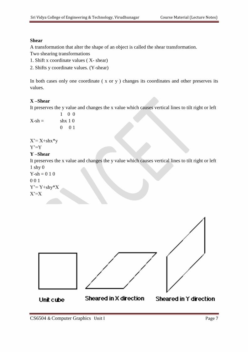
Shear

A transformation that alter the shape of an object is called the shear transformation.

Two shearing transformations

1. Shift x coordinate values ( X- shear)

2. Shifts y coordinate values. (Y-shear)

In both cases only one coordinate ( x or y ) changes its coordinates and other preserves its

values.

X –Shear

It preserves the y value and changes the x value which causes vertical lines to tilt right or left

1 0 0

X-sh = shx 1 0

0 0 1

X’= X+shx*y

Y’=Y

Y –Shear

It preserves the x value and changes the y value which causes vertical lines to tilt right or left

1 shy 0

Y-sh = 0 1 0

0 0 1

Y’= Y+shy*X

X’=X



Shearing Relative to other reference line

We can apply x and y shear transformations relative to other reference lines. In x shear

transformation we can use y reference line and in y shear we can use x reference line.

The transformation matrices for both are given below.

1 shx -shx*yref

X shear with y reference line 0 1 0

0 0 1

x’=x+shx(y-yref) , y’= y

1 0 0

Y shear with x reference line shy 1 -shy*xref

0 0 1

which generates transformed coordinate positions.

x’=x , y’= shy(x-xref)+y

This transformation shifts a coordinate position vertically by an amount proposal to its

distance from the reference line x=x ref.

Transformations between coordinate systems

Transformations between Cartesian coordinate systems are achieved with a sequence of

translate-rotate transformations. One way to specify a new coordinate reference frame is to

give the position of the new coordinate origin and the direction of the new y-axis. The

direction of the new x-axis is then obtained by rotating the y direction vector 90 degree

clockwise. The transformation matrix can be calculated as the concatenation of the translation

that moves the new origin to the old co-ordinate origin and a rotation to align the two sets of

axes. The rotation matrix is obtained from unit vectors in the x and y directions for the new

system

TWO DIMENSIONAL GRAPHICS TRANSFORMATIONS

Composite transformations

- sequence of transformations is called as composite transformation. It is obtained by forming

products of transformation matrices is referred as a concatenation (or) composition of

matrices.

Tranlation : -

Two successive translations

1 0 tx 1 0 tx 1 0 tx1+tx2

0 1 ty 0 1 ty 0 1 ty1+ty2

0 0 1 0 0 1 0 0 1

T(tx1,ty1) + T(tx2,ty2) = T(tx1+tx2, ty1+ty2)

Two successive translations are additive.

Rotations

Two successive rotations are additive.



R(θ1)* R(θ2)= R(θ1+ θ2)

P’=P. R(θ1+ θ2)

Scaling

Sx1 0 0 Sx2 0 0 Sx1.x2 0 0

0 Sy1 0 0 Sy2 0 0 Sy1.y2 0

0 0 1 0 0 1 0 0 1

S(x1,y1).S(x2,y2) = S(sx1.sx2 , sy1.sy2)

the order we perform multiple transforms can matter

eg. translate + scale can differ from scale + translate

eg. rotate + translate can differ from translate + rotate

eg. rotate + scale can differ from scale + rotate (when scale_x differs from

scale_y)

When does M1 + M2 = M2 + M1?

M1 M2

translate translate

Scale Scale

Rotate Rotate

Scale(sx=sy) Rotate

General pivot point rotation Rotation about any selected pivot point (xr,yr) by performing the following sequence of

translate – rotate – translate operations.

1 0 xr Cosθ -Sinθ 0 1 0 -xr

0 1 yr Sinθ Cosθ 0 0 1 -yr

0 0 1 0 0 1 0 0 1

T(xr,yr).R(θ).T(-xr,-yr) = R(xr,yr, θ)

Concatenation properties Matrix multiplication is associative. Transformation products may not be commutative.

Combination of translations, roatations, and scaling can be expressed as

X’ rSxx rSxy trSx X

Y’ rSyx rSyy trSy Y

1 0 0 1 1

Affine transformations Two dimensional geometric transformations are affine transformations. Ie they can be

expressed as a linear function of co-ordinates x and y . Affine transformations transform the

parallel lines to parallel lines and transform finite points to finite points . Geometric

transformations that do not include scaling or shear also preserve angles and lengths.



Raster methods for transformations

Moving blocks of pixels can perform fast raster transformations. This avoids calculating

transformed coordinates for an object and applying scan conversion routines to display the

object at the new position. Three common operations (bitBlts or pixBlts(bit block transfer))

are copy, read, and write. when a block of pixels are moved to a new position in the frame

buffer(block transfer) , we can simply replace the old pixel values or we can combine the

pixel values using Boolean or arithmetic operations. Copying a pixel block to a new location

in the frame buffer carries out raster translations. Raster rotations in multiples of 90 degree

are obtained by manipulating row and column positions of the pixel values in the block.

Other rotations are performed by first mapping rotated pixel areas onto destination positions

in the frame buffer, then calculate the overlap areas. Scaling in raster transformation is also

accomplished by mapping transformed pixel areas to the frame buffer destination positions.

Two dimensional viewing

Two dimensional viewing The viewing pipeline A world coordinate area selected for

display is called a window. An area on a display device to which a window is mapped is

called a view port. The window defines what is to be viewed the view port defines where it is

to be displayed. The mapping of a part of a world coordinate scene to device coordinate is

referred to as viewing transformation. The two d imensional viewing transformation is

referred to as window to view port transformation of windowing transformation.

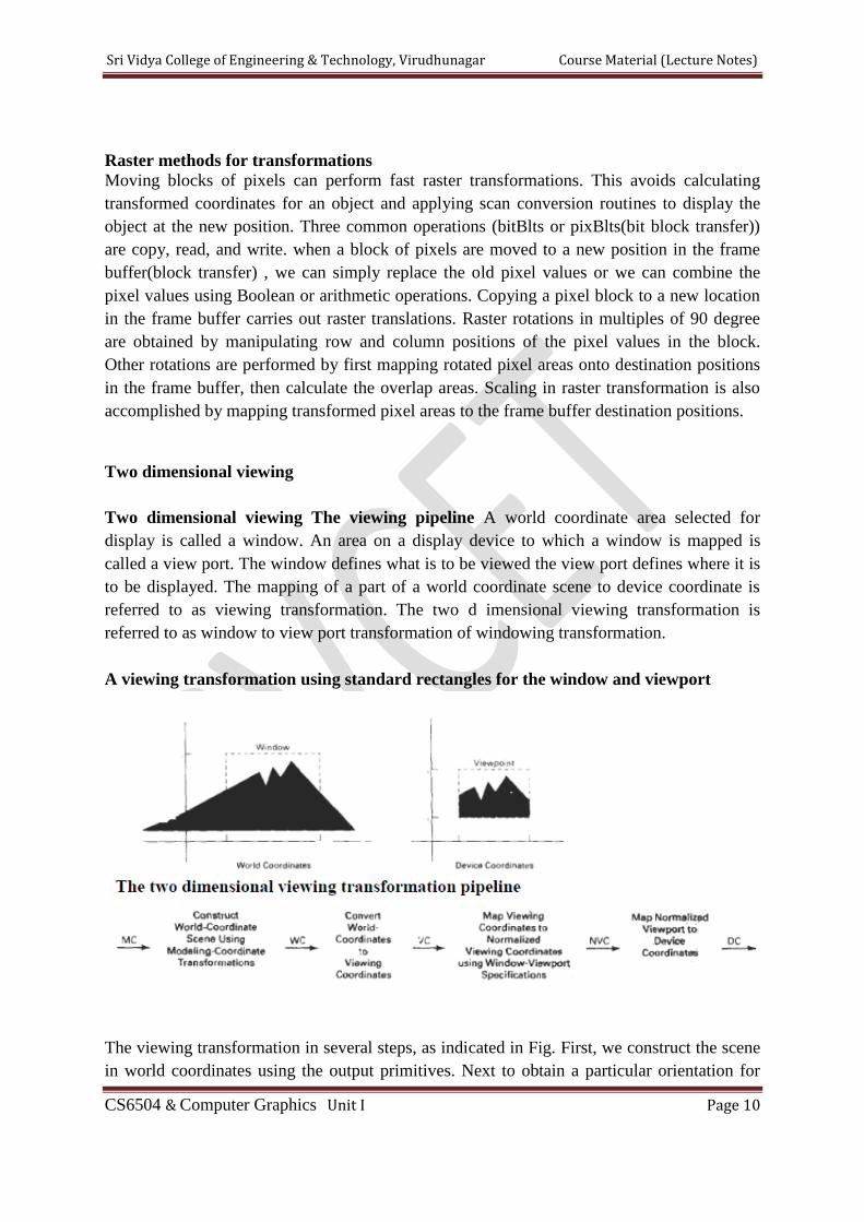
A viewing transformation using standard rectangles for the window and viewport

The viewing transformation in several steps, as indicated in Fig. First, we construct the scene

in world coordinates using the output primitives. Next to obtain a particular orientation for



the window, we can set up a two-dimensional viewing-coordinate system in the world

coordinate plane, and define a window in the viewing-coordinate system. The viewing-

coordinate reference frame is used to provide a method for setting up arbitrary orientations

for rectangular windows. Once the viewing reference frame is established, we can transform

descriptions in world coordinates to viewing coordinates. We then define a viewport in

normalized coordinates (in the range from 0 to 1) and map the viewing-coordinate description

of the scene to normalized coordinates.

At the final step all parts of the picture that lie outside the viewport are clipped, and the

contents of the viewport are transferred to device coordinates. By changing the position of the

viewport, we can view objects at different positions on the display area of an output device.

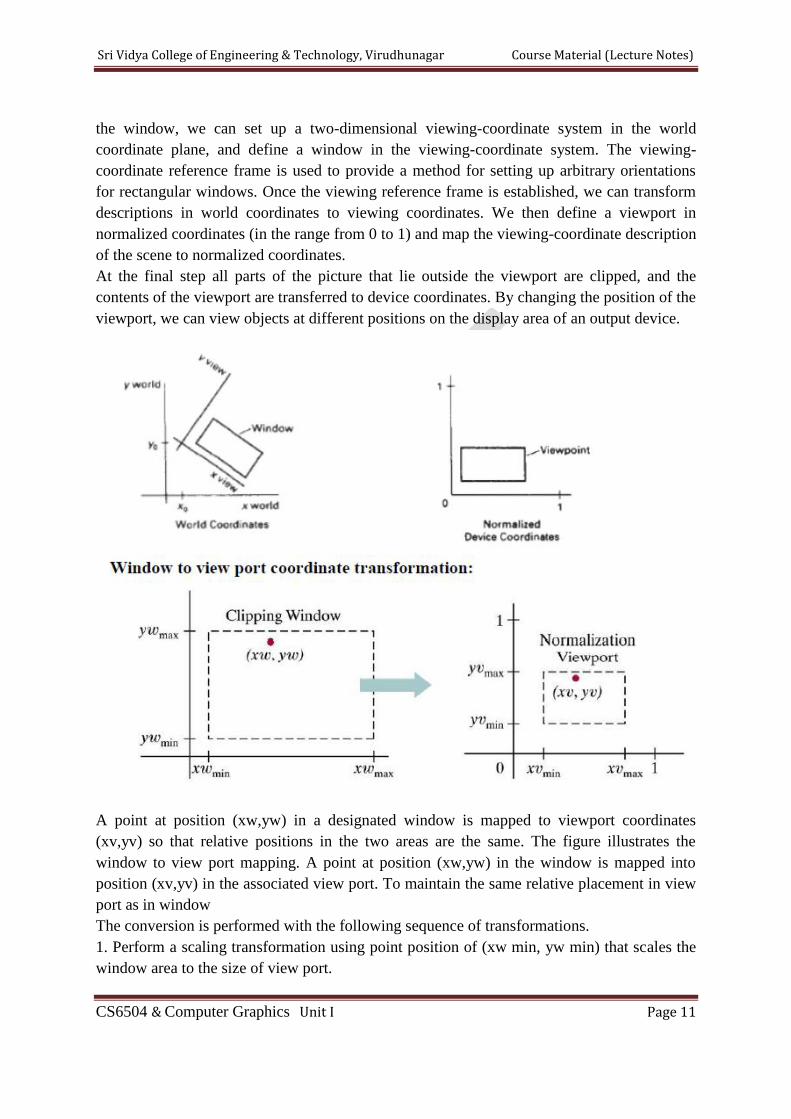
A point at position (xw,yw) in a designated window is mapped to viewport coordinates

(xv,yv) so that relative positions in the two areas are the same. The figure illustrates the

window to view port mapping. A point at position (xw,yw) in the window is mapped into

position (xv,yv) in the associated view port. To maintain the same relative placement in view

port as in window

The conversion is performed with the following sequence of transformations.

1. Perform a scaling transformation using point position of (xw min, yw min) that scales the

window area to the size of view port.



2. Translate the scaled window area to the position of view port. Relative proportions of

objects are maintained if scaling factor are the same(Sx=Sy).

Otherwise world objects will be stretched or contracted in either the x or y direction when

displayed on output device. For normalized coordinates, object descriptions are mapped to

various display devices. Any number of output devices can be open in particular application

and another window view port transformation can be performed for each open output device.

This mapping called the work station transformation is accomplished by selecting a window

area in normalized apace and a view port are in coordinates of display device.

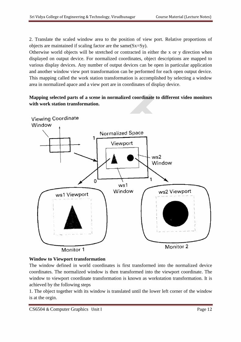
Mapping selected parts of a scene in normalized coordinate to different video monitors

with work station transformation.

Window to Viewport transformation

The window defined in world coordinates is first transformed into the normalized device

coordinates. The normalized window is then transformed into the viewport coordinate. The

window to viewport coordinate transformation is known as workstation transformation. It is

achieved by the following steps

1. The object together with its window is translated until the lower left corner of the window

is at the orgin.



2. Object and window are scaled until the window has the dimensions of the viewport

3. Translate the viewport to its correct position on the screen.

The relation of the window and viewport display is expressed as

XV-XVmin XW-XWmin

-------------- = ----------------

XVmax-XVmin XWmax-XWmin

YV-Yvmin YW-YWmin

-------------- = ----------------

YVmax-YVmin YWmax-YWmin

XV=XVmin + (XW-XWwmin)Sx

YV=YVmin + (YW-YWmin)Sy

XVmax-XVmin

Sx= --------------------

XWmax-Xwmin

YVmax-YVmin

Sy= --------------------

YWmax-YWmin

2D Clipping

The procedure that identifies the portion of a picture that are either inside or outside of a

specified regin of space is referred to as clipping. The regin against which an object is to be

clipped is called a clip window or clipping window.

The clipping algorithm determines which points, lines or portions of lines lie within the

clipping window. These points, lines or portions of lines are retained for display. All other are

discarded.

Possible clipping are

1. Point clipping

2. Line clipping

3. Area clipping

4. Curve Clipping

5. Text Clipping



Point Clipping:

The points are said to be interior to the clipping if

XWmin <= X <=XW max

YWmin <= Y <=YW max

The equal sign indicates that points on the window boundary are included within the window.

Line Clipping:

- The lines are said to be interior to the clipping window, if the two end points of the lines are

interior to the window.

- If the lines are completely right of, completely to the left of, completely above, or

completely below the window, then it is discarded.

- Both end points of the line are exterior to the window, then the line is partially inside and

partially outside the window.The lines which across one or more clipping boundaries requires

calculation of multiple intersection points to decide the visible portion of them.To minimize

the intersection calculation and increase the efficiency of the clipping algorithm, initially

completely visible and invisible lines are identified and then intersection points are calculated

for remaining lines.

There are many clipping algorithms. They are

1.Sutherland and cohen subdivision line clipping algorithm

It is developed by Dan Cohen and Ivan Sutharland. To speed up the processing this algorithm

performs initial tests that reduces the number of intersections that must be calculated.

given a line segment, repeatedly:

1. check for trival acceptance

both

2. check for trivial rejection

both endpoints of the same side of clip rectangle

3. both endpoints outside clip rectangle

divide segment in two where one part can be trivially rejected

Clip rectangle extended into a plane divided into 9 regions . Each region is defined by a

unique 4-bit string

left bit = 1: above top edge (Y > Ymax)

2nd bit = 1: below bottom edge (Y < Ymin)

3rd bit = 1: right of right edge (X > Xmax)

right bit = 1: left of left edge (X < Xmin)

left bit = sign bit of (Ymax - Y)

2nd bit = sign bit of (Y - Ymin)

3rd bit = sign bit of (Xmax - X)

right bit = sign bit of (X - Xmin)



(the sign bit being the most significant bit in the binary representation of the value. This bit is

'1' if the number is negative, and '0' if the number is positive.)

The frame buffer itself, in the center, has code 0000.

1001 | 1000 | 1010

-------------------------

0001 | 0000 | 0010

-------------------------

0101 | 0100 | 0110

For each line segment:

1. each end point is given the 4-bit code of its region

2. repeat until acceptance or rejection

1. if both codes are 0000 -> trivial acceptance

2. if logical AND of codes is not 0000 -> trivial rejection

3. divide line into 2 segments using edge of clip rectangle

1. find an endpoint with code not equal to 0000

2. lines that cannot be identified as completely inside or outside are checked for the

intersection with two boundaries.

3. break the line segment into 2 line segments at the crossed edge

4. forget about the new line segment lying completely outside the clip rectangle

5. draw the line segment which lies within the boundary regin.

2. Mid point subdivision algorithm

If the line partially visible then it is subdivided in two equal parts. The visibility tests are then

applied to each half. This subdivision process is repeated until we get completely visible and

completely invisible line segments.

Mid point sub division algorithm

1. Read two end points of the line P1(x1,x2), P2(x2,y2)

2. Read two corners (left top and right bottom) of the window, say (Wx1,Wy1 and Wx2,

Wy2)

3. Assign region codes for two end points using following steps

Initialize code with bits 0000

Set Bit 1 – if ( x < Wx1 )

Set Bit 2 – if ( x > Wx1 )

Set Bit 3 – if ( y < Wy1)

Set Bit 4 – if ( y > Wy2)

4. Check for visibility of line

a. If region codes for both endpoints are zero then the line is completely visible. Hence draw

the line and go to step 6.



b. If the region codes for endpoints are not zero and the logical ANDing of them is also

nonzero then the line is completely invisible, so reject the line and go to step6

c. If region codes for two end points do not satisfy the condition in 4a and 4b the line is

partially visible.

5. Divide the partially visible line segments in equal parts and repeat steps 3 through 5 for

both subdivided line segments until you get completely visible and completely invisible line

segments.

6. Stop.

This algorithm requires repeated subdivision of line segments and hence many times it is

slower than using direct calculation of the intersection of the line with the clipping window

edge.

3. Liang-Barsky line clipping algorithm

The cohen Sutherland clip algorithm requires the large no of intesection calculations.here this

is reduced. The update parameter requires only one division and windows intersection lines

are computed only once.

The parameter equations are given as

X=x1+ux, Y=Y1 + uy

0<=u<=1, where x =x2-x1 , uy=y2-y1

Algorithm

1. Read the two end points of the line p1(x,y),p2(x2,y2)

2. Read the corners of the window (xwmin,ywmax), (xwmax,ywmin)

3. Calculate the values of the parameter p1,p2,p3,p4 and q1,q2,q3,q4m such that

4. p1= x q1=x1-xwmin

p2= -x q2=xwmax-x1

p3= y q3=y1-ywmin

p4= -y q4=ywmax-y1

5. If pi=0 then that line is parallel to the ith boundary. if qi<0 then the line is completely

outside the boundary. So discard the linesegment and and goto stop.

Else

{

Check whether the line is horizontal or vertical and check the line endpoint with the

corresponding boundaries. If it is within the boundary area then use them to draw a line.

Otherwise use boundary coordinate to draw a line. Goto stop.

}

6. initialize values for U1 and U2 as U1=0,U2=1

7. Calculate the values forU= qi/pi for I=1,2,3,4

8. Select values of qi/pi where pi<0 and assign maximum out of them as u1



9. If (U1<U2)

{

Calculate the endpoints of the clipped line as follows

XX1=X1+u1 x

XX2=X1+u 2x

YY1=Y1+u1 y

YY2=Y1+u 2y

}

10.Stop.

4. Nicholl-lee Nicholl line clipping

It Creates more regions around the clip window. It avoids multiple clipping of an individual

line segment. Compare with the previous algorithms it perform few comparisons and

divisions . It is applied only 2 dimensional clipping. The previous algorithms can be extended

to 3 dimensional clipping.

1. For the line with two end points p1,p2 determine the positions of a point for 9 regions.

Only three regions need to be considered (left,within boundary, left upper corner).

2. If p1 appears any other regions except this, move that point into this region using some

reflection method.

3. Now determine the position of p2 relative to p1. To do this depends on p1 creates some

new region.

a. If both points are inside the region save both points.

b. If p1 inside , p2 outside setup 4 regions. Intersection of appropriate boundary is

calculated depends on the position of p2.

c. If p1 is left of the window, setup 4 regions . L, Lt,Lb,Lr

1. If p2 is in region L, clip the line at the left boundary and save this intersection to p2.

2. If p2 is in region Lt, save the left boundary and save the top boundary.

3. If not any of the 4 regions clip the entire line.

d. If p1 is left above the clip window, setup 4 regions . T, Tr,Lr,Lb

1. If p2 inside the region save point.

2. else determine a unique clip window edge for the intersection calculation.

e. To determine the region of p2 compare the slope of the line to the slope of the

boundaries of the clip regions.

Line clipping using non rectangular clip window

Circles and other curved boundaries clipped regions are possible, but less commonly used.

Clipping algorithm for those curve are slower.

1. Lines clipped against the bounding rectangle of the curved clipping region. Lines outside

the region is completely discarded.



2. End points of the line with circle center distance is calculated . If the squre of the 2 points

less than or equal to the radious then save the line else calculate the intersection point of the

line.

Polygon clipping

Splitting the concave polygon

It uses the vector method , that calculate the edge vector cross products in a counter clock

wise order and note the sign of the z component of the cross products. If any z component

turns out to be negative, the polygon is concave and we can split it along the line of the first

edge vector in the cross product pair.

Sutherland – Hodgeman polygon Clipping Algorithm

1. Read the coordinates of all vertices of the polygon.

2. Read the coordinates of the clipping window.

3. Consider the left edge of the window.

4. Compare the vertices of each edge of the polygon, Individually with the clipping plane.

5. Save the resulting intersections and vertices in the new list of vertices according to four

possible relationships between the edge and the clipping boundary discussed earlier.

6. Repeats the steps 4 and 5 for remaining edges of the clipping window. Each time the

resultant vertices is successively passed the next edge of the clipping window.

7. Stop.

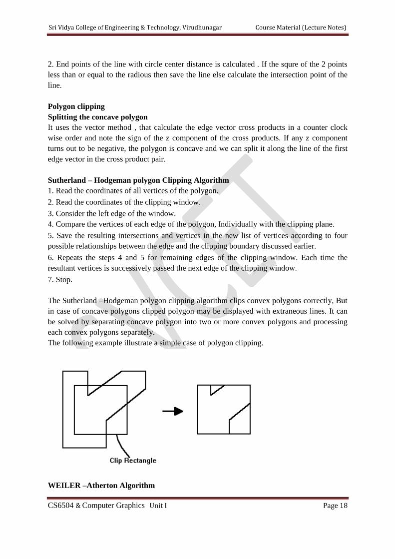
The Sutherland –Hodgeman polygon clipping algorithm clips convex polygons correctly, But

in case of concave polygons clipped polygon may be displayed with extraneous lines. It can

be solved by separating concave polygon into two or more convex polygons and processing

each convex polygons separately.

The following example illustrate a simple case of polygon clipping.

WEILER –Atherton Algorithm



Instead of proceding around the polygon edges as vertices are processed, we sometime wants

to follow the window boundaries.For clockwise processing of polygon vertices, we use the

following rules.

- For an outside to inside pair of vertices, follow the polygon boundary.

- For an inside to outside pair of vertices, follow a window boundary in a clockwise direction.

Curve Clipping

It involves non linear equations. The boundary rectangle is used to test for overlap with a

rectangular clipwindow. If the boundary rectangle for the object is completely inside the

window , then save the object (or) discard the object.If it fails we can use the coordinate

extends of individual quadrants and then octants for preliminary testing before calculating

curve window intersection.

Text Clipping

The simplest method for processing character strings relative to a window boundary is to use

the all or none string clipping strategy. If all the string is inside then accept it else omit it.

We discard only those character that are not completely inside the window. Here the

boundary limits of individual characters are compared to the window.

Exterior clipping

The picture part to be saved are those that are outside the region. This is referred to as

exterior clipping. An application of exterior clipping is in multiple window systems.

Objects within a window are clipped to the interior of that window. When other higher

priority windows overlap these objects , the ojects are also clipped to the exterior of the

overlapping window.

two dimensional graphics transformations geometric ... · two dimensional graphics transformations...

Documents