CALCULATING TEE UNSATUlW'ED HYDRAULIC CONDUCTIVITY WITE A NbW CWSED-FORM

MALYTICAL MODEL

Men van ~enuchten* Water Resources Program

Department of Civil Engineering Princeton University

Princeton, New Jersey 08540

PROPERTY WMT LIBRARY

. . * Present address : U. S . Salinity ~aboratory , USDA, 4500 Glenwood Drive,

Riverside, California 92501.

September 1978

i

A new and r e l a t i ve ly simple equation f o r the s o i l moisture content-

pressure head curve, 8 ( h ) , is described i n this report . The par t icu la r

form of the equation enables one t o derive closed-form &ly t i ca l expres-

sions f o r the r e l a t i ve hydraulic conductivity, Krt when subst i tuted i n

the predict ive conductivity models of Burdine (1953) o r Mualem (1976a).

The resu l t ing expressions f o r K,(h) contain three independent parameters

which may be obtained by f i t t i n g the proposed s o i l moisture re tent ion

model t o experimental data. Two d i f f e ren t methods of curve-fi t t ing a r e

discussed i n the report , a simple but effect ive graphical method, and a

least-squares method requiring computer assistance. An exis t ing non-

l i nea r least-squares curve-f i t t ing program was modified f o r this purpose

and i s included i n an appendix, together with detai led inst ruct ions

regarding i ts use.

Results obtained w i t h the closed form analyt ical expressions based

on the Mualem theory were compared with observed r e l a t i ve hydraulic

conductivity data f o r f i v e s o i l s w i t h a wide range i n hydraulic prop-

e r t i e s . The r e l a t i ve hydraulic conductivity was predicted well i n

four out of f i v e cases. I t was found t h a t a reasonable description

of the s o i l moisture re tent ion curve a t low moisture contents is

necessary i f an accurate prediction of the hydraulic conductivity is t o

be made.

This work was supported, i n part, by funds obtained from the

Solid and Hazardous Waste Research Division, U. S. Environmental Protec-

t ion Agency, ~ h i c i p a l Environmental Research Laboratory, CinciJInati,

Ohio (EPA Grant No. R803827-01) .

iii

A B S T R A C T . . . . . . . . . . . . . . . . . . . . . . . . . . ii.

=ST OF FIGURES . . . . . . . . . . . . . . . . . . . . . . v

LIST OF TABLeS . . . . . . . . . . . . . . . . . . . . . . . vii

MATHEMATICAL DEVELOPMENT . . . . . . . . . . . . . . . . . . 4

PARAMETER ESTIMATION . . . . . . . . . . . . . . . . . . . . 1 6

INFLUENCE OF THE RESIDUAL MOISTURE CONTENT . . . . . . . . . 2 6

RESULTS . . . . . . . . . . . . . . . . . . . . . . . . . . 31

APPENDIX A . . . , . , . . . . . . . . . . . . . . . . . . . 4 4

LIST OF FIGURES

Fig. 1. Typical pXot of the s o i l moisture re tent ion curve based on Eq.

(3)

Fig. 2. P lo t of d e r e l a t i v e hydraulic conductivity versus pressmure

head as predicted from knowledge of the s o i l moisture reten-

t i o n curve shown i a Fig. 1.

Fig. 3. P lo t of tha s o i l moisture d i f fu s iv i t y versus moisture content

as predicted from knowledge of the s o i l moisture re tent ion

curve shown i n Fig. 1, and the hydraulic conductivity a t satu-

ra t ion.

Fig. 4. Comparison of the proposed s o i l hydraulic functions (sol id

l i ne s ) w i t h curves obtained by applying e i t h e r the Mualem

theory (M; dashed l i ne s ) o r the Burdine theoty (9; dashed-

dotted l i ne s ) t o the Brooks and Corey model of the s o i l mois--

t u r e re tent ion e w e .

Fig. 5. P lo t showing the location of the points P, Q, and R on the

s o i l moisture re ten t ion curve. The point P is s i tua ted half-

way between Br (rO.10) and Bs (=0.50), the point Q represents

the i n f l ec t i on po in t of the curve (semilogarithmic p l o t ) , while

R represents the i n f l ec t i on point i f the curve were p lo t ted on

a normal (0 versus h) scale.

Fig. 6. P lo t s of the dimensionless slopes Sp and S a s functions of Q

the parameters n and m (11-l/n).

Fig. 7. P lo t i l l u s t r a t i n g the graphical determination of the para-

meters a and n f o r three d i f f e r en t values of the res idual

moisture content: 8. -0.05 ( s w e a), 0: -0.10 (curve b) , 3 5

and 0: =0.15 a. /a ( m e c ) . The open c i r c l e s represent

the observed s o i l moisture re tent ion curve of S i l t Loam

G. E. 3 (Reisenauer, 1963) .

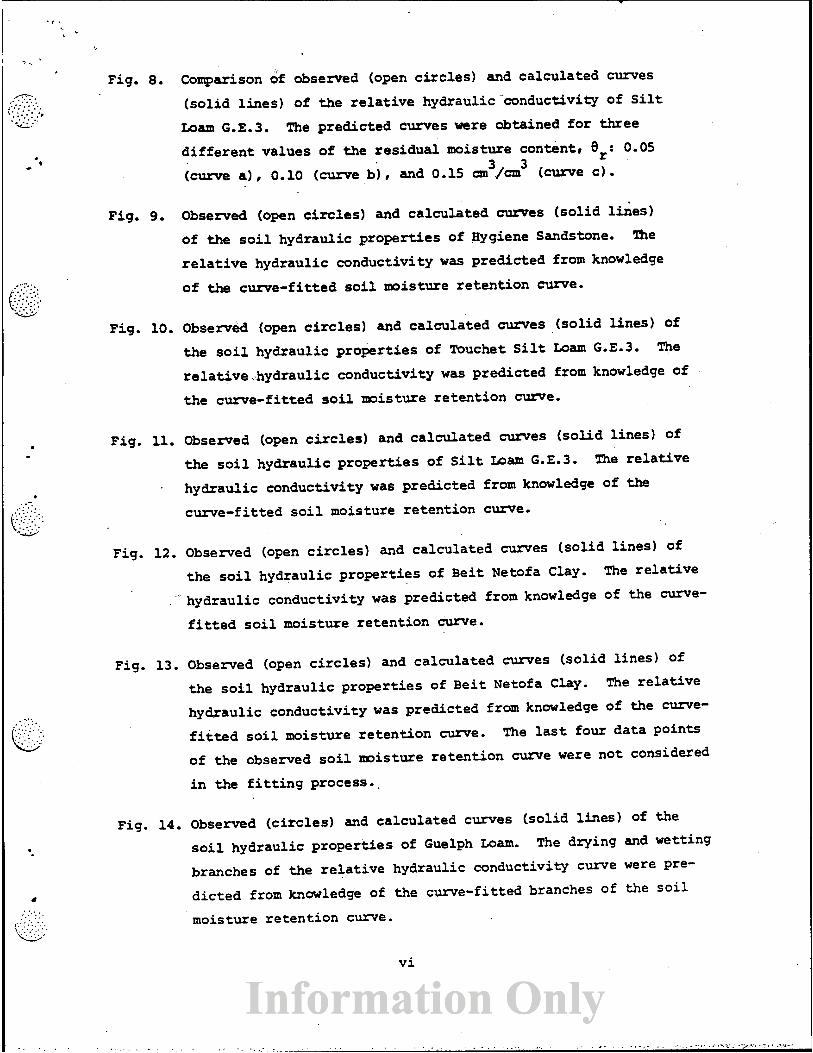
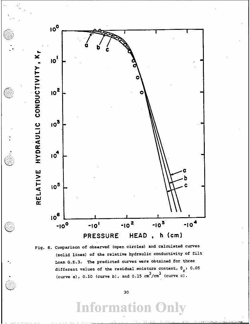
Fig. 8. Comparison of observed (open c i r c l e s ) and calculated curves

( so l id l i n e s ) of the r e l a t i v e hydraulic conductivity of S i l t

Loam G.E.3. The predicted curves were obtained f o r three

d i f f e r e n t values of the res idua l moisture content, er: 0.05 3 ( c u m a), 0.10 ( c w e bj, and 0.15 an / a n 3 ( m e c ) .

Fig. 9. Observed (open c i r c l e s ) and calculated cwPes (so l id l i ne s )

of the s o i l hydraulic p roper t ies of Hygiene Sandstone. The

r e l a t i v e hydraulic conductivity was predicted from knowledge

of the curve-fi t ted s o i l moisture re ten t ion curve.

Fig. 10. Observed (open c i r c l e s ) and calculated curves ( so l id l i ne s ) of

the s o i l hydraulic p roper t ies of Touchet S i l t Loam G.E.3. The

relative. .-hydraulic conductivity was predicted from knowledge of

the curve-fi t ted s o i l moisture re tent ion curve.

Fig. 11. Observed (open c i r c l e s ) and calculated curves ( so l id l i ne s ) of

t he s o i l hydraulic p roper t ies of S i l t Loam G.E.3. %he r e l a t i ve

hydraulic conductivity was predicted from knowledge of the

curve-fi t ted s o i l moisture re tent ion curve.

Fig. 12. Observed (open c i r c l e s ) and calculated curves ( so l id l i ne s ) of

the soil hydraulic p roper t ies of Beit Netofa Clay. The r e l a t i ve

. hydraulic conductivity was predicted from knowledge of the curve-

f i t t e d s o i l moisture re tent ion curve.

Fig. 13. Observed (open c i r c l e s ) and calculated curves (sol id l ines ) of

the s o i l hydraulic proper t ies of Be i t Netofa Clay. The r e l a t i ve

hydraulic conductivity was predicted from knowledge of the curve-

f i t t e d s o i l moisture re tent ion curve. The l a s t four da ta points

of the observed s o i l moisture re ten t ion curve were not considered

i n the f i t t i n g process..

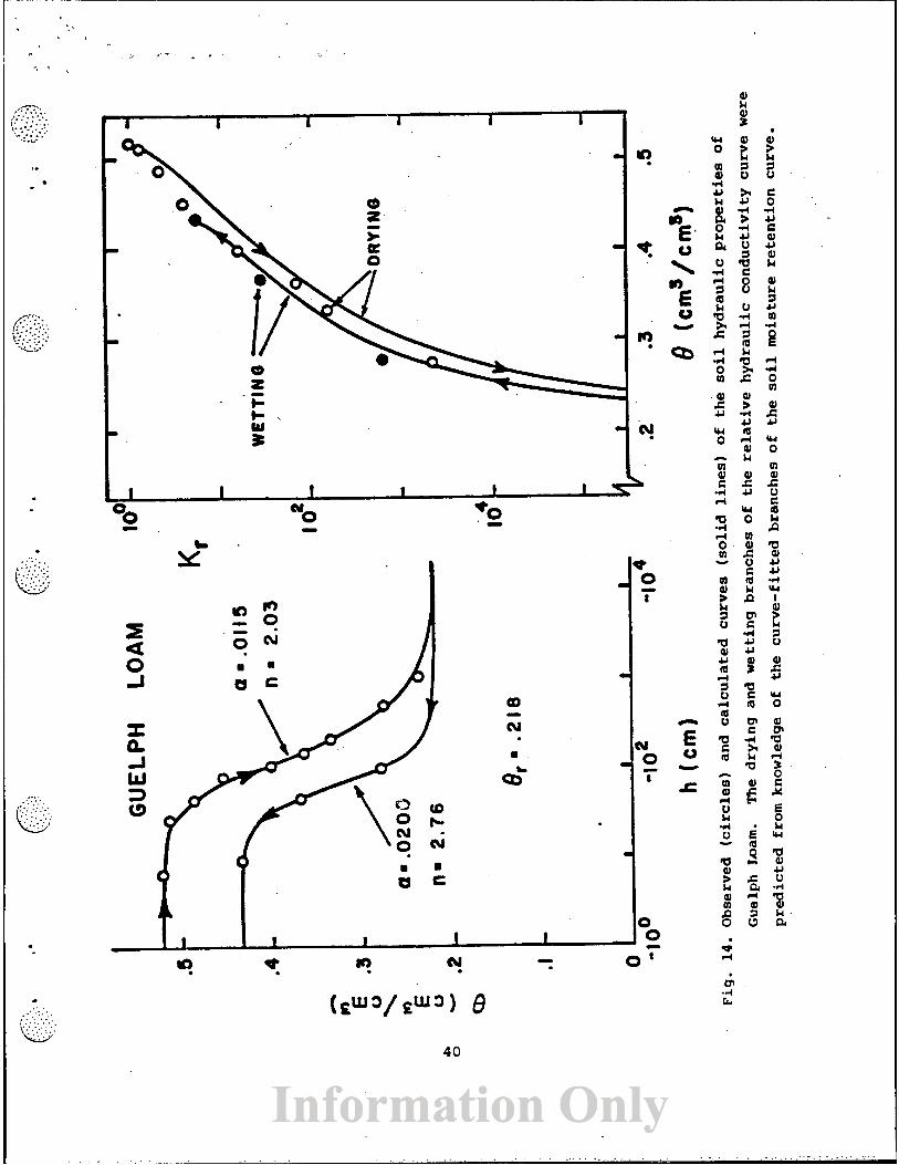
Fig. 14. Observed ( c i r c l e s ) and calculated curves (sol id l i ne s ) of the

s o i l hydraulic p roper t ies of Guelph Loam. The drying and wetting

branches of the r e l a t i ve hydraulic conductivity curve were pre-

d ic ted from knowledge of the curve-fitted branches of the s o i l

moisture re ten t ion curve.

LIST OF TABLES

Table 1. Calculation of the parameters a and n from the observed s o i l

moisture re tent ion curve of S i l t froam G.E.3, using three di f -

f e r e n t values f o r 8, (8s-0.396) . Table 2. Soil-physical proper t ies of the f i ve example so i l s .

Table A l . L i s t of the most s ign i f i can t variables i n SOHYP.

Table A2. Input data ins t ruc t ions f o r SOHYP.

Table A3. Data input f o r example 3 ( S i l t Inam G.E.3) . Table A4. Output fo r example 3 ( S i l t Loam G.E.3) . Table AS. Fortran l i s t i n g of SOHYP.

v i i

The use of numerical models f o r simulating f l u i d flaw and mass

t ransport i n the unsaturated zone has become increasingly popular the l a s t

few years. Recent l i t e r a t u r e indeed dem~ns t r a t e s that much e f fo r t i s pu t

i n t o the development of such models using both f i n i t e di f ference (Bresler,

1975; Amerman, 1976) and f i n i t e element techniques (Reeves and Duguid, 1975;

Segol, 1976). Unfortunately, it appears t h a t the a b i l i t y t o fu l l y charac-

t e r i z e the simulated system has not kept pace with the numerical and model-

ing expertise. Probably the s ing l e most important fac tor l imit ing the

successful application of unsaturated flow theory t o actual f i e l d problems

is the lack of infornration regarding the para-ters 'entering the governing

t ranspor t equations.. Reliable est imates of the unsaturated hydraulic

conductivity a r e espec ia l ly d i f f i c u l t t o obtain, p a r t l y because of its

extensive v a r i a b i l i t y i n t h e . f i e l d , and par t ly because measuring this

parameter is time-consuming and expensive. Several invest igators have,

f o r these reasons, used models f o r calculat ing the unsaturated conductivity

from the more e a s i l y measured s o i l moisture re tent ion curve. Very popular

among these models has been the Millington-Quirk method (Millington and

Quirk, 1961), various forms of which have been applied with some success

i n a number of s tud ies (cf. Jackson et at., 1965; Jackson, 1972; Green and

Corey, 1971; Bruce, 1972). Unfortunately, this method a l so has the dis-

advantage of producing tabula r r e s u l t s which, f o r example when applied t o

nonhomogeneous s o i l s i n multi-dimnsional unsaturated f l w models, a re

qu i te tedious t o use.

Closed-form ana ly t ica l expressions f o r predict ing the unsaturated

hydraulic conductivity have a l s o been developed. For example, Brooks and

Corsy (1964) and Jeppson (1974) each used an analyt ical expression f o r

-the' conductivity based on the Burdine theory (Burdine, 1953) . Brooks

and Corey (1964, 1966) obtained f a i r l y accurate predictions w i t h t h e i r

equations, even though a discont inui ty is present i n the slope of both

the moisture re tent ion curve and the unsaturated hydraulic conductivity

curve a t some negative value of the pressure head (this poin t is of ten

referred t o a s the bubbling pressure). Such a discontinuity sometimes

prevents rapid convergence i n numerical saturated-unsaturated flow prob-

lems. It a l so appears t h a t predict ions based on the Brooks and Corey

equations a re somewhat l e s s accurate than those obtained with vatious

forms of the (modified) Millington-Quirk method.

Recently Mualem (1976a) derived a new model f o r predict ing the hydrau-

l i c conductivity from knowledge of the s o i l moisture re tent ion curve and the

conductivity a t saturation. Mualem's derivation leads t o a s h g l e inte-

g ra l formula f o r the unsaturated hydraulic conductivity which enables

one t o derive closed-form ana ly t ica l expressions, provided su i t ab l e

equations f o r the s o i l moisture re tent ion curves a r e available. It i s

the purpose of this report t o derive such closed-form ana ly t ica l expres-

sions. The theories of both Mualem and Burdine a r e used f o r this deriva-

t ion. The r e su l t i ng conductivity models generally contain three indepen-

dent parameters which may be obtained from the s o i l moisture re tent ion

data by means of cunre-fitting. ' h~o d i f f e r en t methods of curve-fi t t ing

a r e discussed i n this paper, a simple graphical method which enables one

t o obtain the parameters without requiring computer assistance, and a

more e laborate non-linear least-squares curve-fitting method requiring

the ass is tance of a d i g i t a l computer. An ex is t ing computer model was

modified f o r t h i s purpose and is included i n the appendix. Results

obtained with the closed-form equations based on the Mualem theory are

compared with observed data for a few s o i l s having widely varying hydrau-

l i c properties.

' MATHEMATICAL DE7rELOPMGlPT

The following equation was derived by Mualem (1976a) for predict-

ing the r e l a t i v e hydraulic conductivity (Kr) from knowledge of the s o i l

moisture re tent ion curve

'

where h=h(O) i s the pressure head, given here as a function of the dimen-

s ionless moisture content:

I n this equation, s and r indicate saturated and res idual values of the

s o i l moisture content (0) , respectively. To solve ( l ) , an expression

r e l a t i ng the dimensionless moisture content t o the pressure head is needed.

An a t t r a c t i v e c l a s s of O(h)-functions, adopted i n this study, is given by

the following general equation

where a, n and m are as y e t undetermined parameters. To simplify notation

l a t e r , h i n (3) is assumed t o be posi t ive . Equation (3) with m l has

been successfully used i n many s tudies to describe s o i l moisture re-

tent ion data (Ahuja and Schwartzendruber, 1972; Endelman et a l . , 1974;

Haverkanq, e t a t . , 1977). A typical 8 (h) -curve based on Eq. (2) and

(3) i s shown i n Fig. 1. Note t h a t a nearly symmetrical mS"-shaped curve

is obtained, and that the slope (dB/dh) becomes zero when the moisture

content approaches both its saturated and res idual values.

Simple, closed-form expressions f o r \ (a) can be derived when cer-

t a i n r e s t r i c t i o n s a r e imposed upon the values of m and n a l l w e d i n ( 3 ) .

Solving this equation f o r h=h(O) and subs t i tu t ing the resu l t ing expres-

sion i n t o (1) gives

where f (O) i s given by

Subst i tut ion of x=ym i n t o (5) leads t o

Equation (6) represents a par t icu la r form of the Incomplete Beta-function

(see f o r example Abramowitz and Stegun, 1970; p. 944) and, i n its most

general case, no closed-form expression can be derived. However, it is

eas i ly sham that f o r in teger values of k=m-l+l/n the integrat ion can

be carr ied out without d i f f i cu l t i e s . For the par t icu la r case when k=O

(i.e. ~ 1 - l / n ) integrat ion of ( 6 ) yields

6 -10 1 r I I

CL 8, * 0.10 8

-10 = m

CI 4 E -10- 0

- Y

C

0

Q 3 s -10 - m

f:

W a 3 V) V) 2 w -10 - a

a a

I -10 - m

or 0.50

0 - 10 - I I I 1

0 .I 2 3 .4 .5 .6 MOISTURE CONTENT, 8 (crn?crn3)

Fig. 1. Typical plot of the so i l moisture retention curve based on

Eq. ( 3 ) .

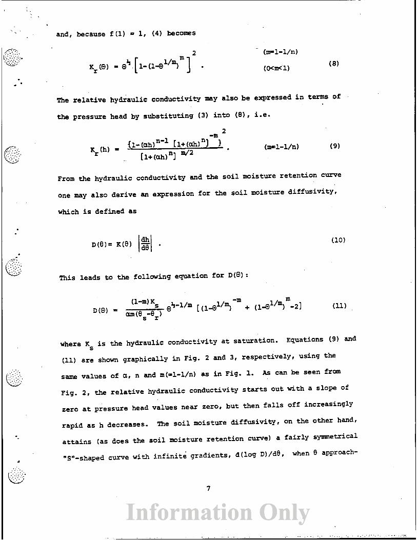
and, because f (1) = 1, (4) becomes

2

xr(W = 0 + [l- (l* l /m)m]

The r e l a t i v e hydraulic conductivity may a l so be expressed i n terms of

the pressure head by subs t i t u t i ng (3) i n t o (81, i .e.

From the hydraulic conductivity and the s o i l moisture re tent ion curve

one may a l so derive an expression fo r the s o i l moisture d i f fu s iv i t y ,

which i s defined a s

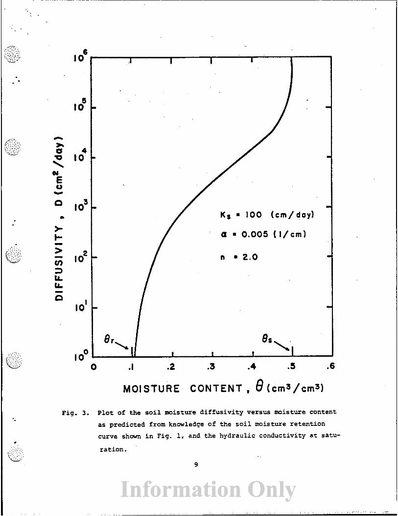
This leads t o the following equation f o r D(@:

where Ks is the hydraulic conductivity a t sa turat ion. Equations (9) and

(11) a r e shown graphically in Fig. 2 and 3, respectively, using t he

same values of a, n and m(=l-l/n) a s i n Fig. 1. As can be seen from

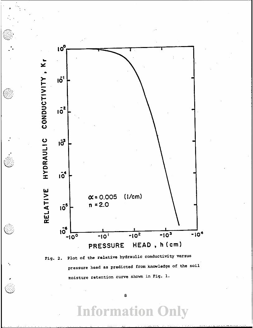
Fig. 2 , the r e l a t i v e hydraulic conductivity starts out with a slope of

zero a t pressure head values near zero, bu t then f a l l s off increasingly

rapid a s h decreases. The s o i l moisture d i f fu s iv i t y , on the other hand,

a t t a i n s (as does the s o i l w i s t u r e re tent ion cunte) a f a i r l y synrmetrical

N S W, shaped curve with i n f i n i t e gradients, d(1og ~ ) / d e , when 0 approach-

PRESSURE HEAD , h ( c m )

Fig. 2. Plot of the relative hydraulic conductivity versus

pressure head as predicted from knwledqe of the s o i l

n;oisture retention curve shown in Fig. 1.

lo"

MOISTURE

Fig. 3. P l o t of the soi l moisture d i f f u s i v i t y versus moisture content

as predicted from knowledce o f the s o i l moisture retention

curve s h m i n Fig. 1, and the hydraulic conductivity a t satu-

rat ion.

e s e i t h e r o r 8 Note t h a t the d i f fus iv i ty becomes i n f i n i t e when 8 ap- s

proaches Bs. Only a t intermediate values of the moisture content (approxi-

mately between 8-0.25 and 8-0.45 i n Fig. 3) does the d i f fus iv i ty acquire

t he of ten assumed exponential dependency on the moisture content.

Similar features of the s o i l moisture d i f fus iv i ty were obtained and

discussed by Ahuja and Schwartzendruber (19721, using the following

spec ia l form of D (8 ) :

where a , p and q a re material charac te r i s t ic parameters.

The s o i l hydraulic proper t ies derived above were obtained by assuming

t h a t k=m-l+l/n=O i n (6). One may a l so derive closed-fonn expressions

f o r other in teger values of k. For k-1, fo r example, the conductivity

becomes

While t h i s pa r t i cu l a r model is not only more complicated than model (81, ,

it a l so represents only a s l i gh t pertubation of the e a r l i e r function.

Hence, (13) does not present an a t t r ac t ive a l te rna t ive f o r (8 ) , and w i l l

no t be discussed further.

Similar r e s u l t s as above fo r the Mualem theory may a l so be obtained

when the Burdine theory i s taken a s a point of departure. The equation

given by Burdine (1953) is:

. . . , . . . . . . . . . . ' . . . . . . , . . . . . . . ' . . . . . . ..... . , . I . . . , _ . . . . . . . . .._: .... ̂ .... i . . . _--. . .

where

Subst i tut ing pym i n t o (16) gives -

Again it i s assumed that the exponent of y i n (171 vanishes. Hence

m=1-2/n, and (17) reduces t o

The r e l a t i ve hydraulic conductivity hence becomes

o r i n terms of the pressure head

-m (ah) n-2 [ i+ (ah) nI

Kr(h) = 2x11 [ l + (ah) "1

:he analysis proceeds i n a similar way as before. Equation (3) is invert- * .

ed t o give h=h@) and subs t i tu t ion of the resu l t ing expression i n t o (14) .c:. ... . . I:..::!;. ;: .. ..' yie lds

,*> '

.

c: : [::.:.... -:..:.;., , . .

. . _ I . -..

-

... . i.;: . <:.:;. .. y;.. : ] -42

-. t. '.', ... ' . ,

.

- . . .'. ' ',. . L: .. . . . . . . .

. : ...,. , . . . . . ... . , ,.. . . . - .. . . . . . . . . . . . . _ . . . _ . . .._ ..,...... . , . ,. ,.. . . ... . . .--., ." .* . . .. - -.-; .-,....,. ,. . - .; . .... . . ' . .... '.. . ..;. ,.,.-. . li

The so i l moisture diffusivity for this case i s given by

Preliminary t e s t s indicated that (8) generated results tha t wefe, i n

most cases, i n better agreement w i t h experimental data than (19) . Through

an extensive series of comparisons, also Mualem (1976a) concluded that pre-

dictions based on his theory (i-e., based directly on Eq. (1) by means of

numerical approximations) were generally msre accurate than those based

on various forms of the Burdine theory (including the Millington-Quirk

method). It is not the intent of this paper to give accuracy comparisons

between various closed-form analytical conductivity expressions. Only a

brief discussion of the equations derived by Brooks and Corey (1964) will

be given here, since thei r model of the s o i l moisture retention curve

represents a limiting case of the moisture retention madel discussed i n

this study.

Brooks and Corey (1964; ,1966) concluded from comparisons w i t h a large

number of experimental data that the so i l moisture retention curve 0(h)

could be described reasonably well w i t h the following general equation

where h, i s the bubbling pressure (approximately equal to the a i r entry

value) , a?d A a s o i l characteristic param?ter- C o ~ a r b 9 ( 2 2 ) and

(3) , one sees that (3) reduces t o (22) for large values of t he pres-

sure head, i .e .

-mn 0 = (ah) .

For the Mualem theory one has -1-l/n, and hence X=n-1, while for the

Burdine theory (nrl-2/n) one finds that A=n-2. The parameter a: further-

more, is inversely related t o the bubblhg pressure, hb. s r w k s and Corey

used the Burdine theory t o predict the r e l a t ive hydraulic conduct i~ i ty and

the s o i l moisture diffusivi ty . They derived the following expressions

-2-3X q ( h 1 = (ah)

Through subst i tut ion of (22) i n t o (11, similar epuations can be obtained ..... . . .

..... when the Mualem theory is used:

Figure 4 compares the d i f fe rent expressions given above w i t h the ea r l i e r

obtained relat ions for the conductivity and the diffusivi ty [Eq. (3) t

(9) and (11) 1. The parameters a and n were chosen t o be the same as

before (i .e. r ~0.005 and n=2) , while A w a s assumed t o be equal to (n-1) -

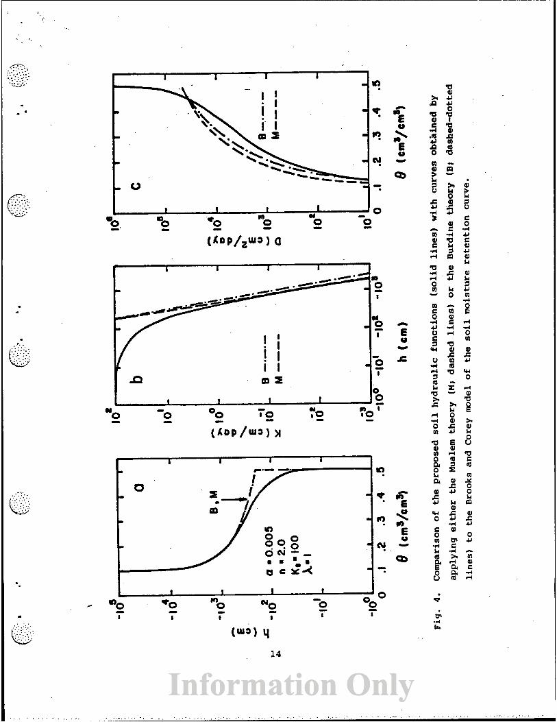
?e s o i l moisture re tent ion curves fo r all three cases become then identi-

c a l f o r su f f i c i en t ly low values of the moisture content. Figure 4a shows

that the Brooks and Corey model of the 0 (h)-curve approaches the curve

based on (3) asymptotically when 8 decreases. However, l a rge deviations

between 'the two models occur then 8 approaches its saturated,value. Ihe

w e s based on (22) reach Bs a t a m c h lower value of h, i.e. a t -200 an

h = a The most important deviations between the predicted conduc-

t i v i t y curves are a l so present a t o r near the bubbling pressure (Fig. 4b).

As expected, the curves based on Eq. (9) and (26b) (the so l id and dashed

l i nes , respectively) approach each other asymptotically when h becomes

increasingly negative, while Me curve used by Brooks and Corey ( the

dashed-dotted l i n e ) remains somewhat separated from the other two because

of the d i f f e r en t exponent i n the conductivity equation [see Eq. (24b) and

(26b)I. The d i f fu s iv i ty curves (Fig. 4c) show their: most important

differences a t both the intermediate and higher values of the moisture

content. Note t h a t the d i f fus iv i ty curves based on (22) remain f i n i t e

(Ds=SO, 000 an2/day) when 9 approaches Bs, while the so l id l i n e (Eq. 10)

goes t o i n f i n i t y a t saturation. It should be emphasized that Fig. 4 was

included only t o demonstrate typ ica l proper t ies of the various conductiv-

i t y and d i f fus iv i ty models, and t h a t the figure should not be viewed a s

an accuracy evaluation of any one model.

The s o i l moisture content (8) as a function of the pressure head

(h) is given by Eq. (2) and (31, i . e . ,

where, as before, it is understood t h a t h is posi t ive , and where fox the

Mualem model

Equation (28) contains four independent parameters (er, es, and n) , which have t o be estimated from obserrred s o i l moisture re tent ion data,

Of these four, t he saturated m i s t u r e content (Be) is probably always

avai lable as it is eas i ly obtained experimentally. Also the res idual

moisture content (8,) may be neasured experimentally, f o r example by de-

termining the moisture content on very d ry so i l . Unfortunately, 0,

measurements are not always made routinely* and hence have t o be estimated

by extrapolat ing ex i s t i ng s o i l moisture re tent ion data. Assuming fo r the

molnent t h a t suf f ic ien t ly accurate estimates of both Br and 8. a r e avail-

able , the following procedure can then be used t o obtair. estimates of the

remaining parameters a and n.

Different ia t ion of (28) gives

where the right-hand s ide is expressed i n tents of Q, rather than h. The

F . pressure head may a l so be expressed i n terms of the-moisture content by *.::-::.: .;, . ... . . L - ... . . . \;.,s--* inver t ing (31, i.e., ,

C I..

.......:

Elimination of a from (29) and (31) r e s u l t s in

The right-hand s ide 'o f this equation contains only the unknown parameta

m (both es and Or are assumed t o be known). Hence it is possible t o o b

t a i n estimates of m by determining the product of the slope (de/dh) and

the pressure head (h) a t some poin t on the 0 ( h ) - m e . So i l moisture re-

ten t ion data are often plotted on a semi-logarithmic scale. One may take

advantage of this f a c t by noting that

d0 de = (In 10) h d (log h)

L e t S be the absolute value of the slope of O w i t h respect t o log h, i .e.,

S = p-1 d (log h)

or , equivalently,

. . - ,

Combining (32), (33), and (34b) leads t o the following expression f o r S

The best locat ion on the 8(h) curve f o r evaluating the slope S i s about

halfiay between Br and 8.. ~ e t P be tha point on the s o i l moisture re-

ten t ion curve fo r which @=+ (see Fig. 5) . From Eq* @) and (31) it

follows then that the coordinates of P are given by

while Eq. (35) reduces t o

The subscr ipt P i n these equations i s used t o indicate evaluation a t P.

Equation (37a) can a l so be expressed i n terms of n

f igure 6 gives a p l o t of Sp a s a function of both n and n. This f igure

MY be used t o obtain an estimate of n once the slope Sp is determined

graphically from the experimental data. For re la t ive ly large values of

n, (37b) is closely approxiwted by

Fig. 5 . Plot showing the location of the points P , Q , and R on the

s o i l moisture retention curve. The point P is situated half-

way between B r (-0.10) and es (e0.50) , the point Q represents

the inf lect ion point of the curve (semilogarithmic p l o t ) , while

R represents the inf lect ion pdint i f the curve were ?lotted on

a normal (8 versus h) scale .

from which one obtains

Alternatively, n can a l so be obtained f r o m (3%) i t s e l f by rearranging the

equation i n t o the following i t e r a t i v e scheme:

The i t e r a t i v e solution converges rapidly. Even f o r a wild i n i t i a l guess of

n generally only two or three i t e r a t i o n s a r e necessaxy t o 0btaj.n answers

correct t o within 19. Once n (or m) is determined, u can be evaluated

with (36b).

An a l te rna t ive approach for estimating n and a from experimental data

f ~ l l a w s by considering the in f lec t ion point on the 0 versus log h curve

(the point marked "Qn i n Fig. 5 ) . Here one has

d20 2

Q 0 . d (log h)

Calculation of the in f lec t ion point is great ly simplified by noting that

d20 Q (In 10) 2

d (log h)

It is eas i ly ver i f ied t h a t subs t i tu t ion of (3 ) i n t o (40) and subsequent

expansion leads t o

Hence, the coordinat6s of the in f lec t ion point are

From (43a) it follows tha t , a t l e a s t theoret ical ly , one could estimate

the value of m d i r ec t ly by locating the in f lec t ion point on the s o i l

moisture re ten t ion curve. However, from Fig. 5 it is clear t h a t it is not

easy t o determine this poin t accurately (even l e s s so when the curve is

based on experimental data) . It seems, therefore, be t t e r t o again esti-

mate m from the slope of the curve. Substi tution of (42) i n to (35) gives

o r , i n terms of n,

Figure 6 shows t h a t Sp(n) and S (n) define approximately the same tun%. Q especial ly f o r the larger n-values. This is not surprising s ince the

points P and Q a re generally very close together on the s o i l moisture re-

tent ion curve. Fig. 5 * f u r t h e m r e , shows tha t both points define approxi-

mately the same gradient. Hence the n-values obtained f r o m the sketched

siope should be nearly iden t ica l .

Instead of using the graphical procedure of Fig. 6 , it is a l so possible

t o obtain n as a function of S by i t e r a t i v e l y solving Eq. (44b) i t s e l f . Q

The following converging scheme was used f o r t h a t purpose:

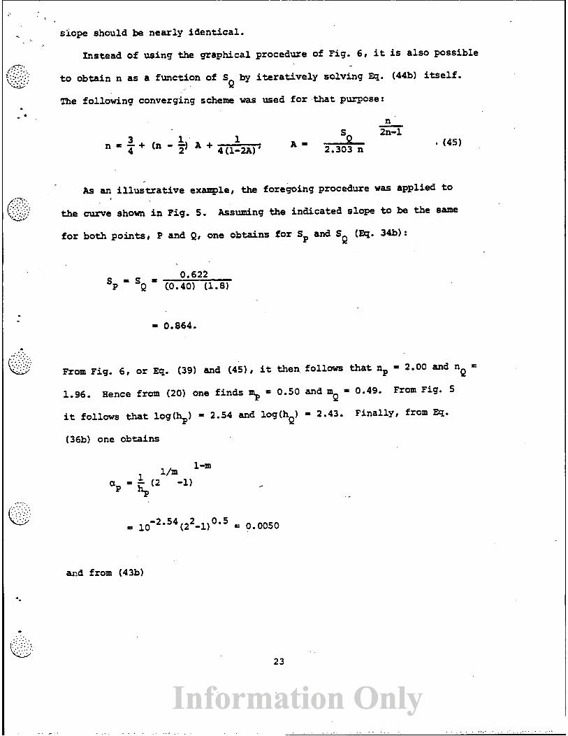
As an i l l u s t r a t i v e example, the foregoing procedure was applied t o

the curve shown i n Fig. 5. Assuming the indicated slope t o be the same

f o r both points, P and Q, one obtains f o r Sp and Sp (Eq. 34b) :

From Fig. 6, o r Eq. (39) and (451 , it then follows that np = 2.00 and n Q

1.96. Hence from ( 2 0 ) one f inds 5 = 0 . 5 0 and m = 0.49. From f ig . 5 Q

it follows that log($) = 2.54 and log(h = 2.43. Finally, from Eq. Q

(36b) one obtains

aEd from (43b)

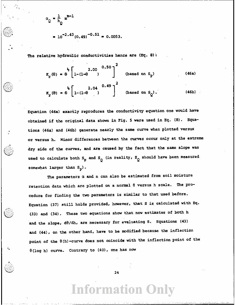
The r e l a t i v e hydrarilic conductivit ies hence e r e (Eq. 8)':

(based on Sp)

(based on S 1 . Q

Equation (46a) exact ly reproduces the conductivity equation one would have

obtained i f the or ig ina l da ta shown i n Fig. 5 were used i n Eq. (8). Equa-

t i o n s (46a) and (46b) generate nearly the same curve when p lo t ted versus

o r versus h. Minor di f ferences between the curves occur only a t the extreme

dry s ide of the curves, and are caused by the fact t h a t t h e same slope was

used t o calculate both Sp and S ( i n r e a l i t y Q s~

should have been measured

somewhat l a rger than Sp) . The parameters a and n can also be estimated from soil moisture

re tent ion data which a re p lo t ted on a normal 8 versus h scale. The pro-

cedure f o r f inding the two parameters is s imilar t o t h a t used before.

Equation (37) sti l l holds provided, however, t h a t S is calculated with Eq.

(33) and (34). These two equations show that now estimates of both h

and the slope, do/&, are necessary f o r evaluating S. Equations (43)

and (44), on the other hand, have t o be modified because the in f lec t ion

po in t of the B(h)-curve does not coincide w i t h the in f lec t ion point of the

0 ( log h) curve. Contrary t o (40) , one has now

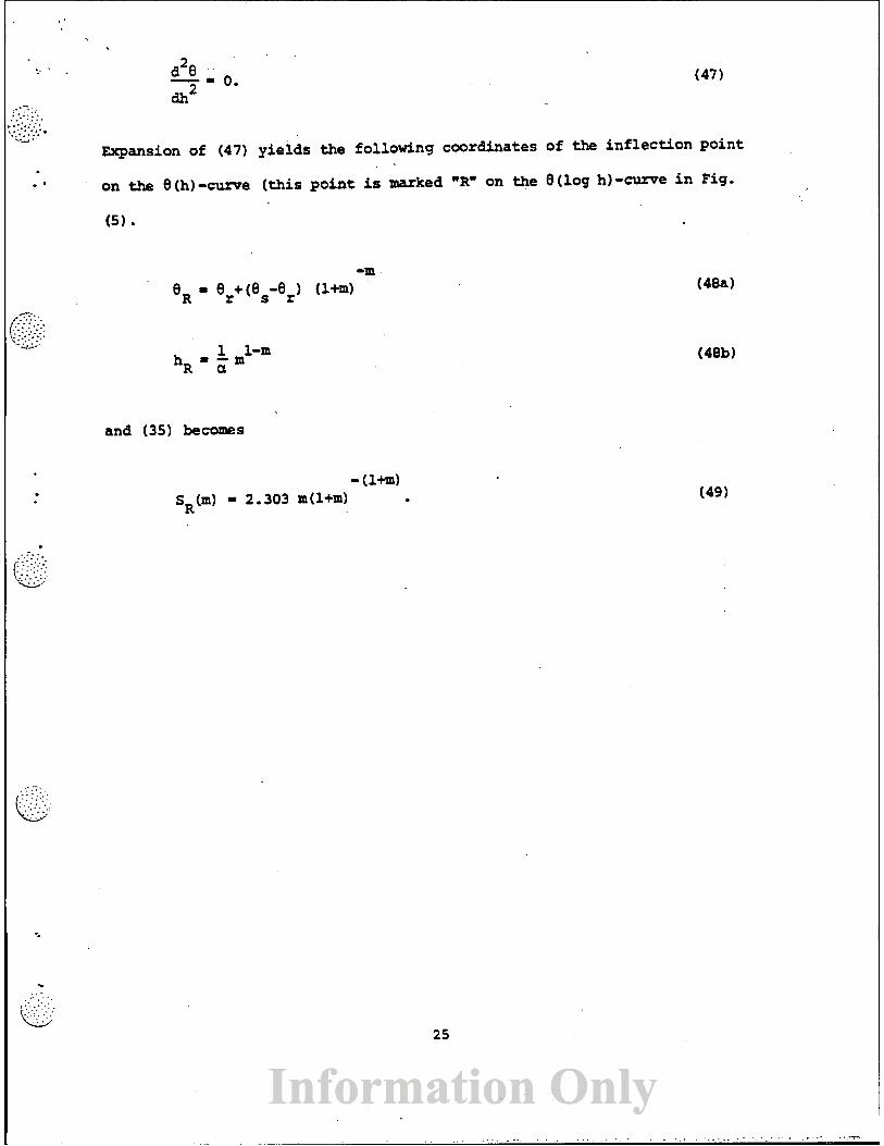
E x ~ M S ~ O ~ of (47) yields the following coordinates of the inflection point

on the B (h) -c-e (this paint is marked nRn on the (log h) -curve i n Fig

(5) .

and (35) becomes

INFLUE'NCE OF THE RESIDUAL MOISTURE CONTKYT

The foregoing discussion assumes t h a t independent measurements

of the saturated and res idual m i s t u r e contents a r e available. While

8. is usually easy t o obtain by d i r e c t measurment, 0, i s of ten much

more d i f f i c u l t t o quantify. In fac t . i n many cases Or m y become ah

i l l-defined parameter. The res idual moisture content i n this repor t

is defined a s the moisture content fo r which the gradient (d8/dh) becomes

zero (excluding the region near Bs which has a l so a zero gradient) . Also

the hydraulic conductivity w i l l approach zero when 8 approaches er. From

a p rac t i ca l po in t of view it seems su f f i c i en t to define as the moisture

content a t some large negative value of the pressure head, e-g., a t -10 -6

cm. Even i n t h a t case, hawever, s ign i f i can t decreases i n h are l ike ly t o

r e s u l t i n fur ther desorption of moisture. It seems t h a t such fur ther

.-- .. .. changes i n 0 a r e f a i r l y uninportant f o r most p rac t i ca l f i e l d problems.

In f a c t , they would be inconsis tent with the general shape of the 8 (h) - curve defined by (22) , and probably inval idate the concept of a res idual

moisture content i t s e l f . A reasonable estimate of er i s necessary f o r

an accurate predict ion of the hydraulic conductivity, even though its in-

fluence on the predictions is generally l e s s than t h a t of a and n. The

following example problem demonstrates the e f f e c t of on the conductivity

predictions.

Figure 7a shows the s o i l moisture re tent ion curve of S i l t Loam

-3 G.E.3, f o r values of h between zero and 10 cm. (Reisenauer, 1963).

The open c i r c l e s represent data polnts of the curve, and were taken from

the catalogue of Mualem (1976b). Because only a l imited portion of the

the curve is defined, an accurate estimate of 8 is not easy t o obtain. r

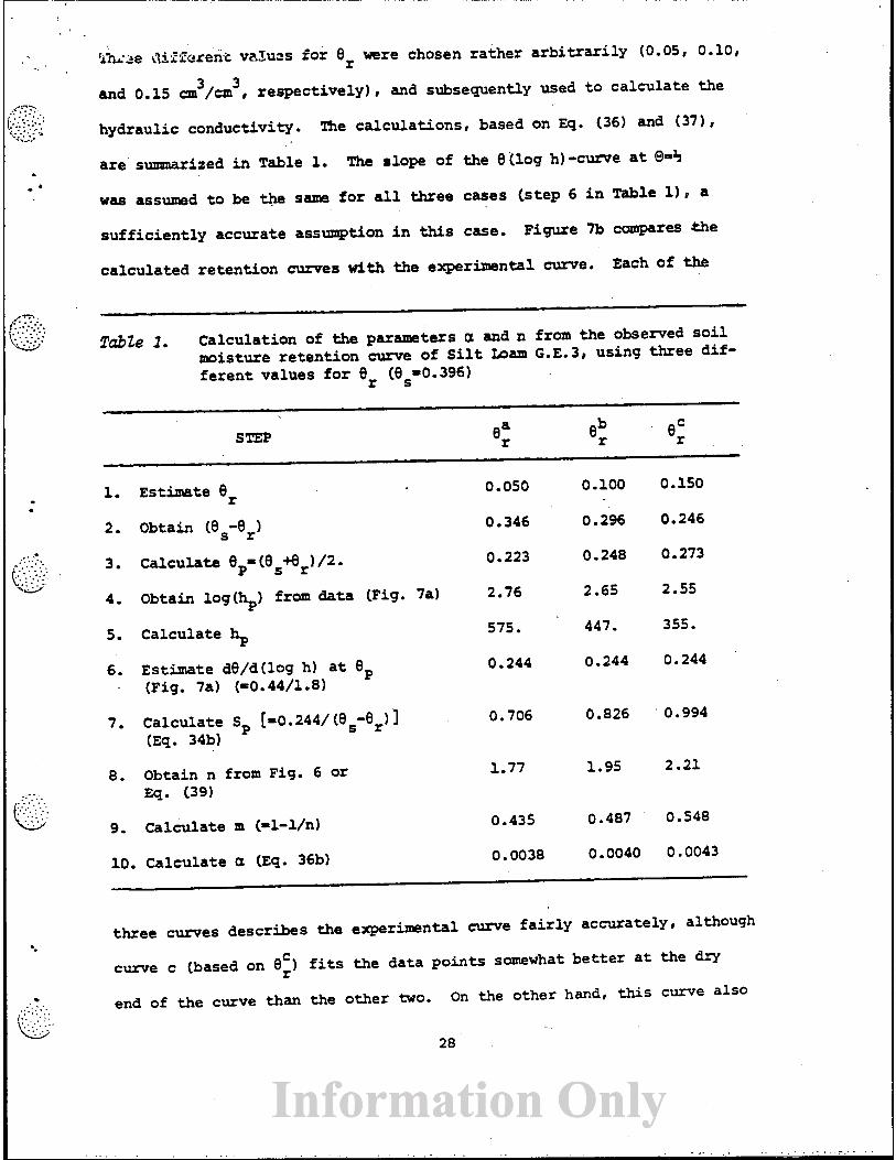
'rhisa diZi'Pareni vaXuzs for 8 were chosen ra ther a r b i t r a r i l y (0.05, 0.10, r 3

and 0.15 cm /d, ~ e s p e c t i v e l y ) , and subsequently used t o calculate the

hydraulic conductivity. The calculat ions , based on Eq. (361 and (37),

a r e summarized in Table 1. The slope of the 8 Uog h)-curve a t

was assumed t o be the same f o r a l l three cases (step 6 i n Table 1) a

su f f i c i en t ly accurate assuxqtion i n this case. Figure 7b compares t h e

calculated re tent ion curves w i t h the experimental curve. Each of the

TabZe 1. Calculation of the parameters a and n from the observed s o i l moisture retent ion curve of S i l t Loam G.E.3, using three d i f - f e r en t values f o r Br (8,=0.396)

STEP

1. Estimate

2. Obtain (eE0er)

4. Obtain log (hp) from data (Fig. 7.1

5. Calculate hp

6. Estimate de/d(log h) a t ep - (Fig. 7a) (=0.44/1.8)

7 . Calculate Sp [=0.244/ (8s-8r) 1 (Eq. 34b)

8. Obtain n from Fig. 6 o r Eq. (39)

10. Calculate a (Eq. 36b) 0.0038 0.0040 0.0043

three curves describes the experimental curve f a i r l y accurately, although

C curve c (based on er) f i t s the data po in ts somewhat be t t e r a t the dry

end of the curve than the other two. On the other hand, t h i s curve also

sl ightly wexpredicts Llw observed o v e a t the higher moisture contents,

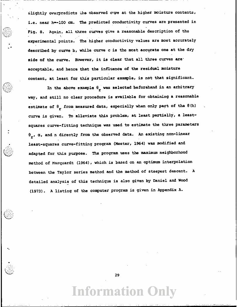
i.e. near h=-100 cm. The predicted conductivity curves are presented i n

Fig. 8. Again, a l l three curves give a reasonable description of the

experimen.ta1 points. The higher conductivity values are most accurately

described by curpe b, while curve c is the most accurate one a t the dry

side of the curve. However, it is clear that a l l three curves are '

acceptable, and hence that the influence of the residual moisture

content, a t leas t for th i s particular example, is not that significant.

In the above example Or was selected beforehand i n an arbitrary

way, and s t i l l no clear procedure is available for obtaining a reasonable

estimate of Or from measured data, especially when only par t of t h ~ B(h)

curve is given. Tb alleviate this problem, a t leas t part ial ly, a least-

squares curve-fitting technique was used t o estimate the three parameters

ex , a, and n direct ly from the observed data. An existing non-linear

least-squares curve-fitting program (Meeter, 1964) was modified and

adapted for this purpose. The program uses the maximum neighborhood

method of Marquardt (19641, which is based on an opt* interpolation

between the Taylor series method and the method of steepest descent. A

detailed analysis of this technique is also given by Daniel and Wood

(1973). A l i s t i ng of the computer program is given i n Appendix A.

PRESSURE HEAD , h (cm)

Fig. 8. Comparison of Gbserved (open circles) an8 calculated curves

(sol id l ines) of the relative hydraulic conductivity of S i l t

Loan. G.E.3 . The predicted curves were obtained for three

different values of the residual moisture content, Or: 0.05 3 3

(curve a ) , 0.10 (curve b), and 0.15 cm /cm (curve c ) .

I n this section comparisons are given between observed and calcu-

lated conductivity curves for five soils. The examples were selected for

soils w i t h widely different hydraulic properties. The observed data for

each example, w i t h the exception of the l a s t one, were taken from the

so i l s catalogue of Mualem (1976b). Table 2 sumarizes sane of the soil-

physical properties of the five soils. Estimates of the parameters e r r

a, and n are also included in the table, and were obtained by fitting

Eq. (28) t o the observed so i l moisture retention data.

Results for Hygiene Sandstone (Brooks and Corey, 1964) are shown

i n Fig. 9. This so i l has a rather narrow pore-size distribution, causing

the so i l moisture release curve t o become very steep around h-125 cm.

A relatively high value of 10.4 for n was obtained for t h i s soi l , a direct

consequence of the steep curve. The value of a was found t o be 0.079

(l/cm), approximately the inverse of the pressure head a t which the so i l

Tabte 2. soil-physical properties of the five example soils.

SOIL NAME

Hygiene sandstone

Touchet S i l t Loam G.E.3 .469

S i l t Loam G.E.3

Guelph Loam (drying) (wetting)

Beit Netofa Clay ,446 ,286 .082 .00202 1.59

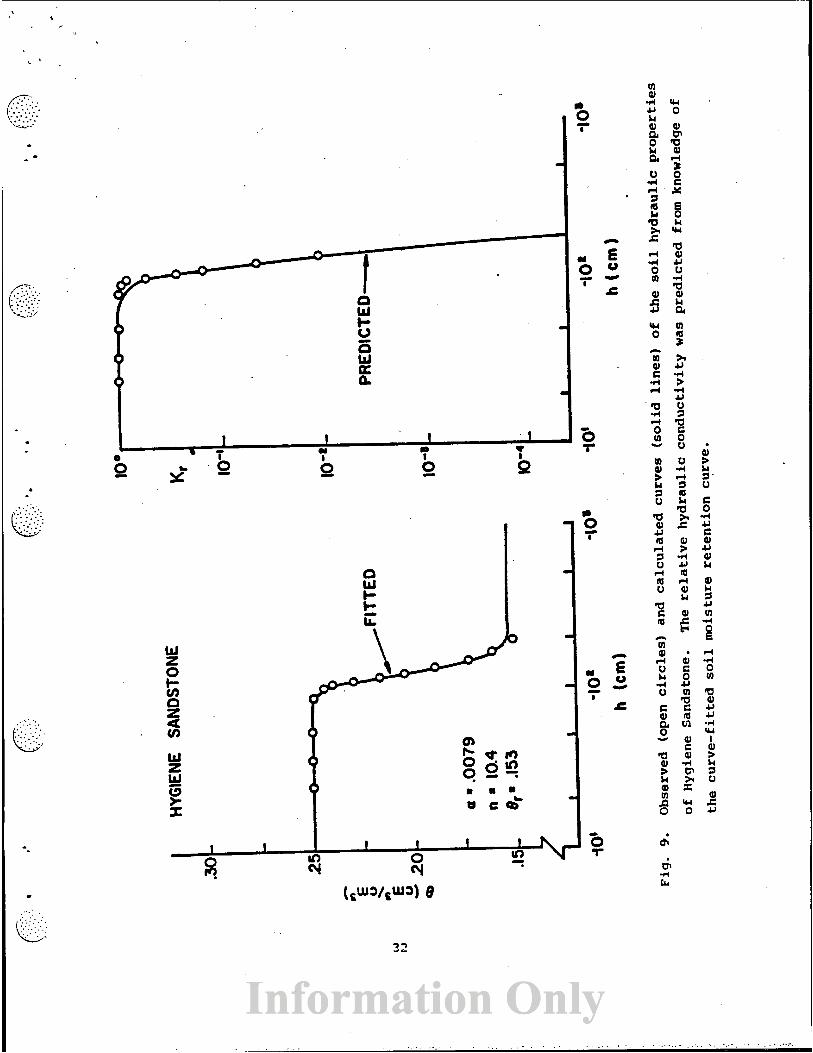
moisture retention curve becomes the s teepes t (Fig. 9 ) . ifiist of course,

follows d i rec t ly from Eq. (36b) and (43b) which, f o r values of m close t o

one (i.e., f o r n la rge) , reduce t o $= hp = l/a. I n that case hp and h Q

both become ident ica l t o the bubbling pressure, %, used in the Brooks

and Corey equations (see Eq. 22 and 23). Fig. 9 shows a nearly exact

prediction of the re la t ive hydraulic conductivity, with only some minor

deviations occurring a t the higher conductivity values.

Results obtained f o r Touchet S i l t Loam G.E. 3 (Brooks and Corey,

19641, sham i n Fig. 10, a r e very similar t o those for Hygiene Sandstone.

The curves i n this case are a l so very s teep (n~7.09)~ and again a good

description of the r e l a t ive hydraulic conductivity is obtained.

Figure 11 presents r e su l t s obtained f o r S i l t Loam G.E.3

(Reisenauer, 1963). This exanple was already discussed i n the previous

section, where estimates of a and n were obtained graphically f o r three

d i f fe rent values of the residual moisture content. I t was then found

t h a t or-values of 0.10 and 0.15 gave the best answers, both for the

description of the s o i l moisture retention curve and the re la t ive hydraul-

i c conductivity. Interest ingly, the three-parameter curve-fitting gave a

value of 0.131, approximately the average of these two or-values.

However, it remains c lear tha t the value of er f o r this par t icu lar

example is poorly defined, and tha t a considerable change i n or w i l l have

only minor e f f ec t s on the calculated curves. Data fo r this s o i l were

a l so used as an i l l u s t r a t i v e exanple for the non-linear least-squares

curve-fit t ing program given i n Appendix A. Output of the program (see

Appendix A) shws t h a t the 95% confidence in terva l for or i s given by

0.131 (+ 16%) . By comparison, these intervals a re .00423 (2 5%) and 2.06

(29%) fo r a and nt respectively. It may be noted here tha t the computer

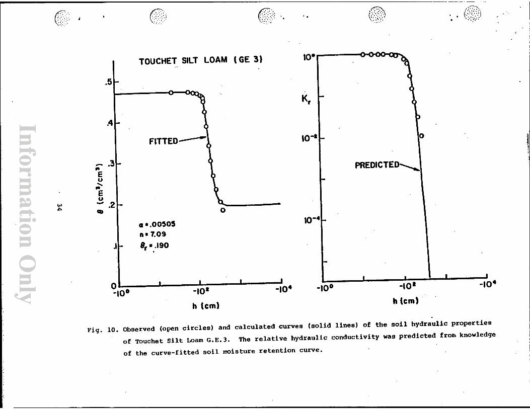
TOUCHET ,. SILT LOAM ( GE 3 )

Fig. 10. Observed (open c i r c l e s ) and ca l cu la ted curves ( s o l i d l i n e s ) o f the soil hydraulic propert ies

o f muchet S i l t Loam G . E . 3 . The r e l a t i v e hydraulic conductivity was predicted fron knowledge

o f the curve- f i t ted soil moisture re t en t ion curve.

I I

'

program also provides for a correlation matrix between the different

parameters. Results, for example, show that er is highly correlated

with n but much less than with a# and that a and n are nearly inde-

pendent of each other. Some of these effects are also noticeable from

the calculations i n Table 1.

The f i r s t three examples each showed excellent agreement &tween

observed and predicted conductivity curves. Predictions obtained for

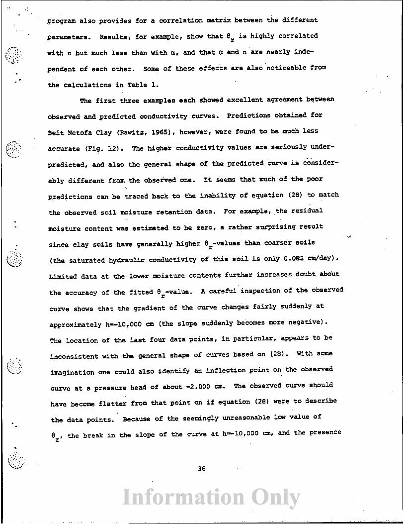
Beit Netofa Clay (Rawitz, 1965): however, were found to be much less

accurate (Fig. 1 2 ) . Ths higher conductivity values are seriously under-

predicted, and also the general shape of the predicted cunre i s consider-

ably different from the obsehed one. It seems that much of the poor

p-redictions can be traced back to the inability of equation (28) to match

the observed so i l moisture retention data. For example, the residual

moisture content was estimated t o be zero, a rather surprising result

since clay soi ls have generally higher 0,-values than coarser soils

(the saturated hydraulic conductivity of this s o i l i s only 0.082 &day).

Limited data a t the lower moisture contents further increases doubt about

the accuracy of the f i t t ed Or-value. A careful inspection of the observed

curve shows that the gradient of the curve changes fa i r ly suddenly a t

approximately h-10,000 cm (the slope suddenly becomes more negative).

The location of the l a s t four data pointsr i n particular, appears to be

inconsistent with the general shape of curves based on (28) . W i t h some

imagination one could also identify an inflection point on the observed

curve a t a pressure head of about -2,000 an. The observed curve should

have become f l a t t e r from that point on i f equation (28) were t o describe

the data points. Because of the seemingly unreasonable low value of

Or: the break in the slope of the curve a t h-10,000 an, and the presence

BElT NETOFA CLAY

Pig. 12. Observed (open c i r c l e s ) and ca lculated curves ( s o l i d l i n e s ) of the soil hydraulic properties

of E e i t Netofa Clay. I h e r e l a t i v e hydraulic conductivity was predicted from knowledge o f the

curve-f i t ted soil moisture retent ion curve.

o f jrn i n f l ec t i on po in t a t h=-2,000 an, an attpmpt was made t o improve the

predict ions by dele t ing rather a r b i t r a r i l y the l a s t four da ta points a t

the dry s ide of the curve. Fig. 13 shows that t h e ' s o i l moisture re tent ion

curve i s now much b e t t e r described (with the obvious exception of t he

last four data poin ts ) . Also the descr ipt ion of the conductivity curve

is *roved somewhat. A t l e a s t the general shape of the curve is described

more accurately, even though the predicted cwve is still displaced t o

t he r i g h t of the observed one. The exanple shcrws t h a t by de le t ing only

four po in t s a t the dry end of the curve a completing d i f f e r en t value of

3 3 - 8, is obtained (0.286 versus 0.0 an /cm ) . This case demonstrates again

the importance of having sonre independent procedure f o r estimating the

res idual moisture content.

Results f o r Guelph -am (Elrick and Bowman, 1964) a r e given i n

Fig. 14. This example represents a case i n which hysteres is is present

in the s o i l moisture re ten t ion m e . The observed data of this example

were taken d i r ec t l y from the or ig ina l study (Figs. 2 and 3 of E l r ick and

Bowman, 1964). For the wett ing branch a maximum ("saturated") value of

0.434 f o r the moisture content was used, being the highest measured value.

Also the wetting branch of the hydraulic conductivity curve w a s matched

t o the highest value of Kr measured during wetting (Fig. 14) . The value

of ere f ~ r t h e r m o r e , was assured t o be the same f o r drying and wetting,

and was 6::-ained from the drying branch of the curve. Both the drying

and wetting branches of the s o i l moisture re tent ion curve are adequately

described by (28). Also the conductivity cunres are reasonably well

descri&dr even though the predicted curves a r e s l i g h t l y below the observed

ones. Note that some hys te res i s is predicted i n t he r e l a t i ve hydraulic

conductivity. Although this is generally t o be expected when t w o d i f fe ren t

BEIT NETOFA CLAY

- L

Pig. 13. Observed (open circles) and ca lcu la ted curves ( s o l i d l i n e s ) of the s o i l hydraul ic p roper t i e s

of Bei t Netofa Clay. me r e l a t i v e hydraul ic conduct iv i ty was p red ic ted from knowledge of

the curve-f i t ted s o i l moisture r e t e n t i o n curve. The l a s t four da ta p o i n t s of the observed

s o i l moisture r e t en t ion curve were no t considered i n t h e f i t t i n g process.

retention cu+v.s 7'i;! drnacnt, FA. (3) also shows that di f ferent retention

curves may generate the same conductivity nwa as long as Or and m (and

hence n) remain the same ( i .e. a may be di f ferent) .

REFERENCES

Abramowitz, M., and I.A. Stegun. 1970. Handbook of mathematical func- t ions . Dover Publ., flew York. 1046 pp.

Atruja, L.R., and D. Swartzendruber. 1972. An improved form of the soil- water d i f f u s i v i t y function. So i l Sci. Soc. Am. Proc. 36(1):9-14.

Ameman, C.R. 1976. Waterflaw in s o i l s : a generalized steady-state, two- dimensional porous media flow model, U.S. Dept. af Agr., ARS-NC-30. 62 PP*

Bresler, E. 1975. Two-dimensional transport of so lu tes k i n g nonsteady i n f i l t r a t i o n fram a t r i c k l e source. S o i l Sci. Soc. Am. P~oc . 39 (4) :604-613.

Brooks, R.H. , and A.T. Corey, 1964. Hydraulic proper t ies of porous media. Hydrology Paper No, 3 , Civ i l Engineering Dept., Colorado S t a t e University, For t Coll ins, Colorado.

Brooks, R.H., and A.T. Corey. 1966. proper t ies of porous media a f fec t ing f l u i d flow. J. I r r i g . Drain. Div., Am. Soc. Civ i l Eng. 92CIR.2): 61-88.

Bruce, R.R. 1972. Hydraulic conductivity evaluation of the s o i l p ro f i l e fram s o i l water re ten t ion re la t ions . S o i l Sci. Soc. Am. Pmc. 36 (4) :555-561.

Burdine, N.T. 1953. Relative permeability calculations f r o m pore-size d i s t r i bu t ion data. Petr . Trans., Am. Ins t . Mining Metall. Eng. 198:71-77.

Daniel, C., and F.S. Wood, 1973. F i t t i n g equations t o data. Wiley-Inter- science, New York. 350 pp.

Endelman, F.J., G.E.P. BOX, J.R. Boyle, R.R. Hughes, D.R. Keeney, M.L. Northup, and P. G. Saf figna, 1974. The mathematical modeling of soil-water- nitrogen phenomena. Oak Ridge National Laboratory. EDE'B-IBP-74-8. 66 PP.

El r ick , D.E., and D.R. Bcwman. 1964. Note on an iqr:>ved apparatus f o r s o i l moisture flow measurements. S o i l Sci. Soc. Am. Proc. 28(3): 450-453 .

Green, R.E., and J.C. Corey. 1971. Calculation of hydraulic conductivity: a fur ther evaluation of some predict ive methods. S o i l Sci. Soc. Am. Proc. 35 (1) : 3-8.

Haverkamp, R., M. Vauclin, J. Touma, P.J. Wierenga, and G. Vachaud. 1977. A comparison of numerical simulation models f o r one-dimensional i n f i l t r a t i o n . S o i l Sci. Soc. Am. J. 41(2):285-294.

Jackson, R.D. 1972. On the calculation of hydraulic conductivity. Soi l Sci. Soc. Am. Proc. 36(2) :380-382.

Jackson, R.D., R. J. Reginato, and C.B.M. van Bavel. 1965. Comparison of measured and calculated hydraulic conductivities of unsaturated so i l s . Water Resour. Res. 1:375-380.

Jeppson, R.W. 1974. Axisymnetric i n f i l t r a t i o n i n so i l s , I. Numerical techniques f o r solution. J. Hydrol. 23:lll-130.

Marquardt, D.W. 1963. An algorithm f o r least-squares estimation 6f non-linear parameters. 3. Soc. Ind. Appl. Math. 11:431-441.

Meeter, D.A. 1964. Non-linear least-squares (Gaushaus). Univ. Wisc. Computing Center. Program revised 1966.

Millington, R.J., and J.P. Quirk. 1961. Permeability of porous solids. Trans. Faraday Soc. 57:1200-1206.

~ u a l & , Y. 1976a. A new model f o r predicting the hydraulic conductivity of unsaturated porous media. Water Resour. Res. 12(3):513-522.

Mualem, Y. 1976b. A catalogue of the hydraulic properties of unsatur- a ted so i l s . Research Project No. 442, Technion, I s r ae l Ins t i tu t e of Technology, Haifa, Israel . 100 pp.

Rawitz, E. 1965. The influence of a number of environmental factors on the ava i lab i l i ty of s o i l moisture t o plants Un Hebrew) . Ph.D. thesis . Hebrew Univ., R e h m t , Israel .

Reeves, M., and J.O. Duguid. 1975. Water movement through saturated- undersaturated porous media: A finite-element galerkin model. Oak Ridge National Laboratory, ORNL-4927. 232 pp.

Reisenauer, A.E. 1963. Methods fo r solving problems of multidimensional p a r t i a l l y saturated steady flaw i n so i l s . J. Geoph. Res. 68(20): 5725-5733.

Segol, G. 1976. A three-dimensional galerkin f i n i t e element model fo r the analysis of contaminant transport i n variably saturated porous media. User's guide. Dept. of Earth Sciences, Univ. of Waterloo, Canada. 172 pp.

A COMPUTER MODEL FOR CALCULATmG

THE SOIL HYDRAULIC PROPERTIES

FROM SOIL MOISTURE RETENTION DATA.

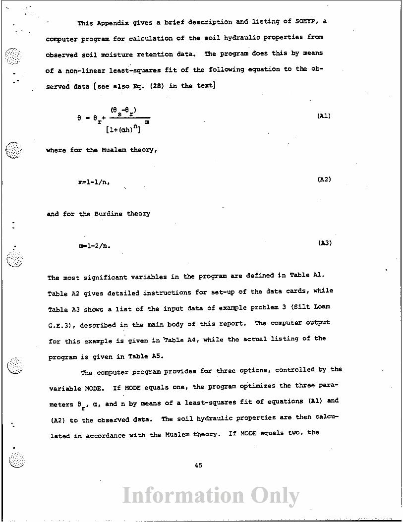
This Appendix gives a brief description and l i s t ing of SOHYP, a

computer program for calculation of the s o i l hydraulic properties from <.'; C ....

I . . . . . . . .;.. . - :. ..:: .' . . .. ,..I... . ... . . .-

observed so i l moisture retention data. The program does th i s by means

of a non-linear least-squares f i t of the following equation to the ob-

served data [see also Eq. (28) in the -1

<.:.:.:.., c;., . . t.. :: .. . . ._.: where for the Mualem theory,

qnd for the Burdine theory

The most significant variables i n the program are defined i n Table A l .

Table A2 gives detailed instructions for set-up of the data cards, while

Table A3 shaws a list of the input data of example problem 3 (Si l t Loam

G.E.3) , described i n the main body of this report. The computer output

for this example i s given in able A4, while the actual l i s t ing of the

program is given i n Table AS.

The computer program provides for three options, controlled by the

variable MODE. If MODE equals one, the program optimizes the three para-

meters Or, a, and n by means of a least-squares f i t of equations (All and

(A21 t o t h e observed data. The so i l hydraulic properties are then calcu-

lated i n accordance with the Mualem theory. If MODE equals two, the

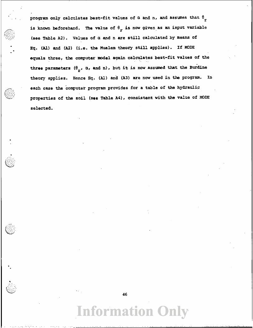
program only calculates best-fit values of a and n , and assumes that 0 r

i s known beforehand. The value of er is now given as an input variable

(see Table A 2 ) . Values of a and n are still calculated by means of

Eq. (All and (A2) (i.e. the Mualem theory s t i l l applies). ~f MODE

equals three, the computer M e 1 again calculates best-f i t values of the

three parameters (er, a, and n) , but it is now assumed that the ~ k d i n e

theory applies, Hence Eq. (Al) and (A3) are now used i n the program. In

each case the =onputer program provides for a table of the hydraulic

properties of the s o i l (see Table A4), consistent w i t h the value of MODE

selected.

Table A I .

VARIABLE

Lis t of the most s i p i f i c a n t var iables i n SOHYP.

Hydraulic conductivity (K).

Coefficient a i n Eq. (All . Array containing i n i t i a l estimates of coeff ic ients .

Array of coef f ic ien t names.

S o i l moisture d i f fu s iv i ty (D) . MIT

MODE

MODEL

NC

NDATA

NIT

NOB

RK

RM

RN

RWC

SATK

SSQ, SUME

Maximum number of i t e ra t ions .

Designates model type t o be used i n program:

1 : Wee-par-ter f i t (er, a, and n) (~ua lem theory)

-2 : m-parameter f i t (a, n) (Mualem theory)

3 Three-parameter f i t (Or, a, n) ( ~ u d i n e thmrl) . Subroutine t o calculate s o i l moisture content (8) from

pressure head (Eq. a)

N u m b e r of cases considered.

Input da ta code:

PO: New da ta a r e read i n

=l: Data from previous case a r e used,

I t e r a t ion number during program execution.

N u m b e r of observed data points (must not exceed 40) .

Relative hydraulic conductivity (Kr) .

Equals l- l /n for Mualem theory, l-2/n f o r Burdine theory.

Coefficient n i n Eq. (All.

Dimensionless moisture content (@) . Hydraulic conductivity a t sa turat ion ( K ~ ) .

Residual sum of squares.

STOPCR

TITIE (I)

WC

WCR

WCS

X ( 1 )

Stop Criterion. Iteration process stops when the

relative change i n each coefficient beccaples less t han

Array containing information of t i t l e cards.

Volumetric moisture content (8) . Residual misture content (er) . Saturated moisture content (es).

Array of observed pressure heads (values are assumed to

be positive) . Y (1) Array of observed moistwe contents.

. L

TABLE A1 (CONTINUED): . -

,p?- .: , ;.:. ..>. . ..:. .. I. .,.. . .' .: &::

.

p (.-;::.::{, -.- . \....... e'

. . :; .. :.. \:;::;:,:

.. . ' . .:.

* . '. _ . . . . . . . .. . L

. . . . . . . . . . . . . . . . . . . . . - . -.

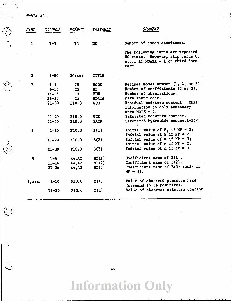
Tab Ze A2.

CARD -

Number of cases considered.

The following cards a r e repeated NC times. However, skip' cards 6, etc., i f NDATA = 1 on t h i r d data card.

20(A4) TITLE

Defines model number (1, 2, o r 3). Number of c o e f f i c i e n t s (2 o r 3). Number of observations. Data input code. Residual moisture content. This information is only pecessary when MODE = 2. Saturated moisture content. Saturated hydraulic conductivity.

MODE NP lOOB ND AT A WCR

WCS S ATK

I n i t i a l va lue of er i f NP 3; I n i t i a l value of a i f NP = 2. I n i t i a l value of a i f NF' = 3; I n i t i a l value of n i f NP = 2. I n i t i a l value of n i f NP = 3.

Coeff ic ient name of B (1) . Coeff ic ient name of B(2). Coeff ic ient name of B(3) (only i f NP = 3).

Value of observed pressure head (assumed t o be pos i t ive ) . Value of observed moisture content.

? d ~ e -43. Input data for example 3 (Silt Loam G.E.3).

1 2 3 4 - 5 Column: 12345678901234567890123456789012345678901234567890

Card

1 SILT LOAM G.E.3

1 3 1 3 0 0.18 0.180 0.002 2.3

WCR ALPHA N 10.0 0.396 20.0 0.394 43.0 0.390 60.0 0.3855 80.0 0.379 . 111.0 0.370 190.0 \ 0.340 285.0 0.300 400.0 0.260 600.0 0.220 800.0 0.200 900.0 0.194 1000.0 0.190

Table A4. Output for example 3 (Silt Loam G.E.3).

'34 3crl 3 C P

X I " ??

do - m a m C I a I =: o m * z n 3 * 4 0 I I . eon* - r d o m m t m 0 . . a m 4 0 0 4 m Ly m a I a ~ r d c u m 0 1 U I

w m w t r 3-0s d N d S * l n 3 . 4 . 0 . m n w m r a U J I I d g N a n c I

a l * II zu - m L L L L I I a e d m

II !US05 r r 033'9 '" "0.35 - u . . i n n U 3 Q S ) r m . A r .a a N 2 l a m

PRESSURE 0.0 Ool41E 0 1 0.168E 0 1 O.2UOE 0 1 0.237E 0 1 0.282E 0 1 Oe335E 0 1 0.399E 0 1 0.473E 0 1 0.562E 0 1 0e668E 0 1 0e794f 0 1 0.944E 0 1 O.112E 0 2 0.133t 02 O.151E 02 O.18dE 02 O.224f 0 2 O.266E 02 Om3lbE 02 0.376E 0 2 0m447E 02 0.531E 0 2 Omri3lE 92 0.750E 0 2 0.891E 02 0. AObE 03 0.12bL 03 0.150E 03 O.178E 03 0e211E 03 0.251E 0 3 0.259E 03 0.355t 03 0.4LZf 03 0.501E 03 0.596E 03 Om7OBE 03 OmB41E 03 0.100E 0 4

LOG P HC & E L n LOG RK AUS ~k LOG K A DL FFUS LUG o 0.3960 O.130E 01 0m496E 0 1 0.3960 3m9YlE 00 -0 .004 . 0.4926 0 1 0.692 OoY39E O b 5.913 0. 3960 O.YUYE CO -0.005 0e491E 0 1 0.691 O.781E 0 6 5.U93 0.3969 0e967E 0 0 -0.006 Oe4FOE 0 1 0.690 0.649E 0 6 5.812 0.3963 O.985E 0 0 -0.001 0e488E 0 1 Oe089 0.534i 06 5.732 0.3969 O . Y ~ L E 0 0 -3.008 0 . 4 ~ 7 ~ 0 1 0.661 o . e c e ~ us 5.651 0.3960 3eY71E 00 -0.010 O.482c 0 1 0.686 0e37AE 0 6 5.570 0.3960 0e974E 03 -3.012 0.483E 0 1 0.684 0.308E 06 5m4Ud 0.3960 O e 9 b B E 0 0 -0.014 0.480t U l 0.682 0 . ~ 5 5 f 06 5.431 0.3959 Oe962C 0 0 -0.017 Oo477E 0 1 0.679 0.2115 9 6 5.325 0.3959 0.955E 00 -0.020 3.473E O l 0.675 0.17iE 0 6 5 . ~ 4 2 0.3959 0 . 9 4 6 ~ 00 - 0 . 0 ~ 4 O . ~ ~ Y E 01 0.a11 o . l e 4 ~ 06 s . ~ s a 0.3958 0e935E 0 0 -0.029 0.464E 0 1 Oe6bb O.119E 36 5.074 0.3957 O.Y22i 0 0 -0.035 0.4576 0 1 0.160 3.975E 35 4.909 0.3956 OeVO7E 0 0 -0.043 0.45UE 01 0.653 0.800ti 0 5 4.903 0.3955 Oed88E 0 0 -0.051 Om44lE 0 1 0.644 0.654E US 4.815 0.3953 0.867E 00 -0. C62 O.43UE 01 0.633 00332E 0 5 4.726 0.3949 0eB41E 00 -Om075 0.417E 0 1 0.620 O.432E 05 4.635 0.3945 O o B l l E OU -0.091 Oe4OLE 0 1 0e63f 003+8E 05 * a 5 0 2 0.3933 01775E 00 -0.111 0.3dCE 3 1 0.585 OoLlLE 0 5 4.446 0.3930 0.135E 0 0 -0.134 0.364E 0 1 0.561 0.2LLE 05 4.347 0. 391 l 9 . 6 8 6 ~ 03 -3.164 0 . 3 4 0 ~ 3 1 0.532 0 . 1 7 6 ~ 35 4.245 Om3899 00631E 0 0 -0.200 0.313E 01 0.496 OelJ7t 0 5 4.191 0.3874 0e57UE 00 -0.244 0.2U3E 01 0.451 0. 13bE 0 5 4.tJ26 0.3610 0.502E 0 0 -0.299 OmZ43E 0 1 0.396 O.UllE 0 4 3e9U9 0.3794 0e433E 00 -0.367 O.Ll3E 01 0.329 O.6LLE34 3.7tJb 0.3732 0.355E 0 0 -0.450 0.176E 0 1 0.246 0.453E U4 3eb>b 0.3650 3.28LE 03 -0.551 0 . A392 01 0.144 0e330E 04 3m5Lli b.3547 3.212E 30 -0.675 ' 0.135E 0 1 0.021 0.236E 34 3.373 0.342 1 0.151E 03 -0.822 3.747E 00 -O* l27 0 . 1 6 6 ~ 0 4 3.221 0.3272 OolOlE OU -0.996 0.5UOE OU -0.331 0al15E 34 3 r 0 ~ l 0.3105 0.634E-01 -1.198 00315E 0 0 -0.532 Oe7Y3E 0 3 2.894 Om 2926 0.375E-01 -1.426 0.186E OIJ -0.#30 0 . 5 2 6 ~ 03 2.721 0.2743 Oe210E-01 -1.678 0.104E 0 0 -0.983 0.34YE 0 3 2.943 0.2563 0.112E-01 -1.953 0.553E-01 -1.257 OeZ>OE U3 2.361 0.2391 0.569E-02 -2.245 00292E-31 -1.549 0.15UE03 2,176 0.2238 Oo281E-02 -2.551 Om139E-01 -1.636 0.97.3E 92 1.998 0.2100 0.135E-02 -2.869 00673E-02 -2.174 0.629E OL 1.19ti Oml97d 0.637E-03 -3.196 0m31bE-02 -2.500 O0405E 0 2 1-608 0.1873 0.2966-03 -3.529 Om 147E-02 -2.633 U.260E 0 2 1.416

Tabte AS. Fortran l i s t ing of SOHYP.

MAIN

****r*l******f****S*****t***u**+#*+************ 8 8

* NCN-LI NEAR LEAST-SQUARES ANALYSIS OF SOHYP * 8 SOIL HYORAUL IC PROPERT IES 'APRIL 1980

* * * * * * * t * * * * * * * * * * * * * * * * * + * * * * * ~ t * * t * * r n * * * * * * * * * * * * ~ ~ * s ~ * * * * * w * *

--- REAC NUMBER OF CASES CONSIDERED - REbD(5,lOOO) NC DC 144 IC=lrNC REbOISr10C21 TITLE WRlTE(br1004) TITLE

----- READ INPUT PARAMETERS --- REb0(5r1000) WCDE, hPTNOB~NDATAeWCR~WCS~SATK WRITE16~1005) CCDETNP,NOBTYCRIUCS*SATK

----- READ INZTIAL EST1 HATES -- READ(SrlOC61 (B(I )rI=lrNP)

----- REAC COEFFICIENTS NAMES -- NB I =2*NP RE10(5~1007) ( B I ~ X ) T I ~ ~ T N B I )

-- REbC bN0 WRITE EXPERIPENTAL DATA - WRITE(6r 10081 IF(NCAT~.CT.OJ GO TO a 00 4 I=lrNOB

4 REPC(SrlOC6) X(I)tY(Ih 8 00 10 I=l,NOB

1 0 YRITE(6rlOLl) IrX(IJrY( I I C C --.-.-I

00 12 IllrNP 12 TH(I1-B(I)

IFt(NP-Zl*(NP-3)) 14e16e14 14 URITE(6r1016)

GO TC 142 16 G A ~ O e O Z

CALL MOOEL~THTF~NOBTX~WCS,MODE VNPT WCR)

lF~RODEoNEo2) WRI TE(6rIO26) NITtB(1J tB(Z),B(3J tSSQtnOOE

----- BEGIN OF ITERATION - 34 NTT=NIT+l

GAmO l 1*GA 00 38 J-ltNP TERP-tn (J 8 fH(J)~laOl*TH~J) 01 J)-0 CALL M O D E L ( T H ~ O E L L ( ~ ~ J ~ ~ N O B ~ X ~ W C S ~ ~ O O E ~ N P ~ ~ C R ~ D O 36 I=lrNGB OELZ(I,JI=DELZ(IIJ)-F(I1

36 Q4JltQLJ)+DELZ(f,J)*R(I) Q(J1~100o*CIJIlTH~J)

C C --- STEEPEST CESCENT -

38 TH(Jl*TEMP DO 44 ImlrNP 00 42 J=l11 SUC=O 00 40 K=l,NOB

40 SUP~SUM+OELZ(K~I)*OELZ~K~JI O(I,J)=lOOOO.*SUH/(fn(f)*fHIJ)D

42 O(JtI)fD(ItJ) C C --- 0 = M ~ ~ E N T MATRIX --

44 E( 1)tSQRT (O(1,I)) SO 00 52 I*ltNP

00 52 J-1tNP 52 A(I,JI=D(ItJ)/(EiI)*E(J)) - --- A IS THE SCALED ROMENT NATRIX --

00 54 I=l,NP P(1)-O(f )/Eli) PHI(I)=P(I)

54 AlfrI)~A(ItI)*Gb CALL MATINV(AtNPtP)

----- PIE IS THE CORRECT ION VECTOR - ST EPsl. 0

56 DO S 8 Ir1,NP 5 8 TQtI J=P( I)*ST EP/E( I)+TH(I)

00 62 f=l,NP IF (THt 1 )*TB(I) 166~66962

62 CONTINUE sune=ooo CALL MOOELITBrF tNOB,X,WCS,HaDE,NPvYCR) 00 64 ImltNcB R ( 1 1-Y(1I-F(f1

64 SUH0=SUMB+R(I)*R(Il 66 sunl=o.o

s U)r2*0.0 s UN3-0.0 DO 68 I*lrNP

S U ~ I = S U ~ ~ + P ~ I )*PHI (1) SUHZ=SUN2+P(I)*PlIl

68 SUC3=SUM3+PHItfl*PHtCI) ANGLE*S7~29578*ARCOSCSUMl/S4RT(SUMZ*SUH3))

C C ----

DO 72 I-leNP IF(TH(1 )*tB(I) 174174172

72 CCKTINUE IF(SUMB/SSQ-I.O)BOI~O~?~

74 I F(AYGLEo3000 176*761?8 76 STEP=STEP/2oO

GO TO 56 78 GA=lO.*GA

G O TO 50 C c - - PRIRT COEFFICIENTS AFTER EACH ITERATION --

80 CONTINUE 00 82 1-lrNP

8 2 tHII)=TB(I) IF(!!ODEoEC-ZI WRITE(6.1026) N f T t ~ C R p TH(~)~TH(ZJ tSUM8tMOOE IF(YOOEoNEo2) kRlTE(6r1026J ~ NIT~TH(~J~TH(ZJ *TH(~I#SURB~HODE fF(MODEmECe2J GO TO 90 IF(TH(lJ.CTo6o005~ GO 70 90 WRfTE(6rlO20) GO TO 144

90 00 92 I=l,NP IF(b8S(PtI)*STEP/E(I ))/C1.0EZO+A8StTH( I) J J S C '92,92996

9 2 CONTINUE GO TO 96

94 SSQ=SUMB IF(NIToLEoH1T) GO TO 34

C C ----- END OF ITERATION LOOP --

96 CONTINUE , CALL FAT INV (D*NP*Pl

C c ----- WRITE CORAELAT ION NATRIX ---

DO 98 I'lvNP 98 ElI)~SORT~D(IrI))

YRITE(6rlC44J I IvI'lrNP1 00 102 IsIINP DO 100 J-lr I

100 A(JTI)=D(JII)/(E~I).E(J)J 102 WRIfE(6,lCbB) Ir(A(J*I)rJ~lrI)

C C --- CALCUCAT E 95Z CONFIDENCE INTERVAL ---

Z ~ ~ O / F L O A T (hG8-KPJ SDEV=SQRT(Z+SUR8) wRITE(6rlOS2 J T vAR=l. 96+~*(2.3779*2.( 2.7 13S+Z* (3.181936+2~466666*Z**ZJ J 8 DO 108 1-lrNP SECOEF- E t I )*SDEV TVbtUE= Th(I)/SECCEF

TSEC-TVAR*SECOEF TMCO!?-T:~~( 1 J-TSEC TPCOE=THIIJ*TSEC K= 2* I 3-U-1

108 CRfTEf6tlOJBI B I ( J J ~ B Z ( K J ~ T H ~ I J~SECDEF,TVALUE~TMCOE~TPCDE C C ----- PREPARE FINAL O n P U f --

LSCRTt 11-1 00 116 Jm2,NOB T EHP-R( J J K= J-1 DO ill L=lrK LL=LSORt (L) IF(TEMP-RILL)) 1121112,111

Ll1 CCNfINUE LS tRT4 J)=J G O T 0 1 1 6 -

112 KK-J 113 KKsKK-1

LSCRT(KK+lJ=LS0RTlKKJ IF (KK-LI 1 1 ~ ~ l l s t l ~

115 LSCRT(L1-J 116 COHTlNUE

WRITE(6,lObbl 00 118 IrltNOB

C c ----- URITE SOIL HYDRAULIC PROPERTIES -

dRfTE ( 6 9 1069) PSESS=lm 1885 0 RNltOoO SKLN= 1. O WR!T E(6, 1072) RNl,YCS,RKLNpSATK 03 140 1=1,7S IF(RKLN.LT.(-16o)I GO 7 0 142 PRESS=l.l8@50*PRESS. IF(MODE-2) 120*122r120

120 kCR=TH( 1 J bLPHP.-TH( Z J RNtTHf 31 GO t(! 124

122 ALPHA-TH(1J RN-TH(21

124 RM-lm-1-/RN IF (HODE.EQ.3) RM-lo-ZolRN RN l=ilM*RN RuCtl./( ~.+(ALPHP*PRESS)**RN~**R~~

- .

TERM=~.-RHC*(ALPHA-PRESS)**RNL ~Fl~T€RH.LT.~~~-05).0R0~R~C0LT~Oe06)) TERM Rq*RwC**(le/RH)

M A I N

TERM=hLPHA*RNl*(WCS-YCR)*RYC*RWC**(I,/RNj*(ALPHA*PR€SS)**(RN-Zm) AK=SATK*RK OlFFUS-AK/TERM PRLN-ALOGlO (PRESS) AKLN=ALOGlO(AK) RKLN=ALOGlO(RK) OIFtN=ALOGlQ~O1fFUS)

140 ~RITE(6r 10701 PRESSIPRLN~YC,RK,RKLN~AK~AKLN~DIFFUS~DIFCN '

142 CONTINUE 144 CONTINUE

C C --- END OF PROBLW - 1000 FORMAT(4ISrSf 1OmOJ

I 1002 FORMAT(tOb4) 1004 FOQMAT( 1Hl rlOX,82( lH*)/llX.lH* / l r X * 9x9 'NON-LINEbR LEA

1st SQUARES A N A L Y S I S * r 3 B X ~ l H * / 1 U ~ l H * ~ 8 O X t l H * / l l X ~ 1 H * ~ 2 O A 4 ~ ~ ~ * / ~ ~ ~ ~ 21H* rBQXl lH*/llX,82(lH*)

1005 FQRNATl//ll)lt81NPUT PMAMETERS'/llX,l6(1H~)/ 2llXr'MOOEL N U M 0 E R m . m ~ r m o m ~ ~ m m ~ o ~ o e ~ ~ m m e ~ o m ~ e o m a m ~ ~ m m e m ' ~ I 3 ~

311X.'.NUUBER GF C O E F F I C f E N T S m m ~ ~ . e m m . m ~ ~ m o r m o o . e m m . m ~ a m * ~ I 3 / 411X.'NUHBER 3F ~ ~ S E R V A T I O N S ~ I . ~ O ~ . . ~ O ~ ~ ~ ~ ~ ~ ~ ~ ~ ~ ~ ~ ~ O ~ ~ ~ ' * I ~ ~ SllX, 'RESIDUAL MGISTURE CUNTENT (FOR MOEL Z)mmomooo'rFIO.4/ 611X,'SATURITED MOISTURE C O N T E N t r m m m m m a o o o m . o m o m m m e m ' t F 1 0 ~ 4 I 711Xp'SATURATED HYORAULIC CONDUCTIV1TYeer.mmrmemmm.m'~f10m4J

1006 FORMAT (4F 10.0) 1007 FORRAT(C(b4*P2*4XJJ 1008 F9RUAf(/llLX,*OBSERVEO O A T A @ ~ / l ~ X ~ l 3 ~ l H ~ l / 1 1 X ~ ~ O B S m NOm8r4X,'PRESS

1URE HEAO',ZX.'MCISTURE CONTENT*) 1011 F O R M A T ( ~ ~ X * I ~ ~ ~ X I F ~ ~ ~ ~ P ~ X ~ F ~ Z ~ ~ ~ 1016 FORMAT (//5XpIO( ltl* )t ' ERROR: INCORRECT NUMBER 3F COEFFICIENTS' ) 1026 FORNATilSX r 12 ~ l O X , F B r 4 , 3 X , F l O m 6 ~ 2 ~ ~ F l O e 4 ~ 5 X ~ F 120794Xt 14) 1028 FOPMAT(//llX,'WCR If LESS THAN 0.005, USE TWO-PARAMETER MODEL NfTH

1 WCR OmO'l 1030 F O P M A T ~ l H 1 ~ 1 O X ~ ' I T U ( A T I O N NO*r8X~'YCR'~8Xt*ALPHA',LOX~'N'~13X~'fSO

1' ,8X.'MOOEL@ J 1044 FORMAT(//llX~'CO~REtATION M~fftIX'/llX~l8(1H~)/l4~~10~4X~~2tfX)~ 1048 F O f i M A T ~ l W ~ I 3 ~ l O ( Z X ~ F 7 e 4 ~ 2 X l ~ 1052 FORMA~(//~~X~'NCN-LINEAR LEAST-SQUARES ANALYSIS: FINAL RESULTS'/

lllXp48(lH~J/64Xt'55% CONFIDENCE LlHIf S'/llXt 'VARIABLE' *8X,'VALUE8 o 27Xt'SoEmCCEFFo' *3Xe'T-VALUE',6Xt 'LOHER'~1O%~'UPPER8 I

1058 F O R M A T ~ A ~ X , A ~ , A ~ ~ ~ X , F ~ O ~ ~ . 1066 FOPMAt(//lOX*B(lH-),'ORDERED BY COMPUTER 1NPUf'v 8(LH-)* 7X110(1H-

1) t 'OROEREO eY RESIDUALS' t LO( lH-)/26X* 'MOISTURE CONTENT' 93x1 ' RESf-' 1*24X~'MOlSTURE CONTENT'~~X~'RESI~'/~OX~'KO',~X~'PRESSURZ'~SX~'O~S' 2*4X,'FIfTED'*QX*'DUaL'r 9X*'NO*p3X~'PRESSURE'~SX,'O8S'~4X*'fITTED' 3,4X*'DUAL')

1068 FORMAT (lOX~tt~FlO.2~ lX~3F9~4,BXt I t ~ F l O e Z ~ l X ~ 3 F 9 m ~ ~ lC69 FORMAT(lHlplOX~'PRESSURE',4X,'LOG P1r6X,'~C'*7X,'REL K'rSXv'LOG RK

1' t6X.lA8S K'r4Xt'LOG KA' ~SXI'DSFFUS' *SXt*LOG 0' ) 1070 FOR~AT(lOX*ElO~3.FBm3~f 10.4~34 E1313eFB13)l 1072 F O R M A T ( I O X ~ E l O m 3 ~ B X ~ F l O o 4 . E13m 39 8XvE13-3)

STOP END

HAT I N V

SUBRJUIINE MATINVIA,NPrBJ DIMENSION Ai3.3) r d ( 3 ) r l N D E X l 3 r t 0 DO 2 511.4

2 I N D E X I J r l I = O 1-0

4 AHAX--1.0 00 i 10 J-1 9NP I F ( INDEX1 J, 1) J 1 3 r 6 r 1 0

6 00 10 K-1,NP I F ( I N D E X ( K 9 1 J ) 13r i J r 10

8 PmABSIA(J r& I IFIPmLEmAMAX) GQ T3 13 fR=J IC-K AWAX-P

10 CONTIkUE IF (AnAX) 3 0 9 3 0 ~ 1 4

14 INDEX1 l C r l J = I R I F ( 1 i l a E Q - I t ) GO TO 1 8 00 16 L - l vNP Q t A ( I R r L ) A( I R r L ) - A l It rL J

16 A( IC rL )=P P=0( I R B(1R J=B(IC) BL IC)=P I=I+l INDEX1 I r Z ) = I C

18 P=lm/A( I C r I C ) A( 1 C . I C J - t ~ ~ 00 2 0 L = l r N P

20 A( I C r L ) = A ( ICeL) *P 8f 1C)=6 i 1C)*P 00 24 K s l v N P I F I K a E Q a I C ) GO T J 24 P=A(Ke I C J AtKeICI-Om0 00 22 L-1rNP

22 A ~ K ~ L J ~ A ( K ~ L I - A ( I C r M B[K)=B iKJ-B t IC) *P

24 CONTINUE GO TO 4

26 IC=INDEXI 192 ) IR=INDEXI I C 9 1 ) 00 2 8 K r l r N P P=A( K r I R J ' ( K r I R l * A ( K t I C I

28 A(Kr1C)aP I f 1-1

30 I F I I J Z b e 3 2 r 2 6 32 RETURN

END

SUBROUTINE HODEt(6 , FY, NO09 XIWCSV~DOE~NPVYCRJ D l M E N S I 3 N 0 4 3 1 r F Y 4 4 O J r X t 4 G J

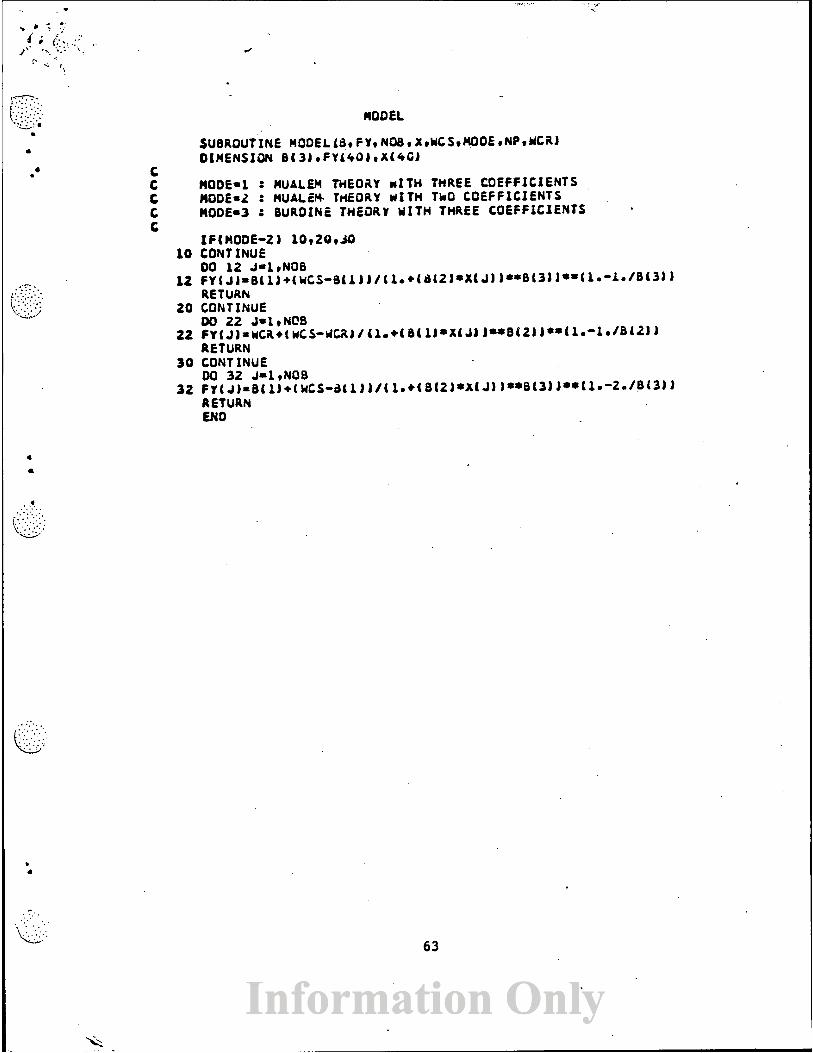
ROOE-1 : MUALEn THEOAY n t T H THREE C O E f f I C t E N T S RODE=L : MUALEK THEORY WITH TLO COEFFICXENTS MODE=3 t BURDINC THE3RY Y I T H THREE COEFFICIENTS

10 CONTINUE DO 12 J * l t N O B

12 F Y ~ J J ~ B l l J + l W C S ~ 8 ~ 1 J J / l 1 o + ~ d l 2 J * X I J J J * * B ~ 3 ~ J * * ~ l a ~ l ~ l B l 3 J ~ RETURN

20 CON1 I N U E 00 22 J = l r N @ B

22 C Y ( J ) = Y C ~ + ( W C S - ~ ~ J ~ ~ ~ ~ + ( B ~ l ) * ~ t J j J**BI2J J * * ( l * - l m l B i 2 J ) RE1 URN

30 CON1 XNUE

RETURN EN 0