propeller-nacelle aerodynamic performance prediction · propeller-nacelle aerodynamic performance...
TRANSCRIPT

NASA Contractor Report 4199
An Analysis for High Speed Propeller-Nacelle Aerodynamic Performance Prediction
Vo Znme I I - User's M UHUU Z
T. Alan Egolf, Olof L. Anderson, David E. Edwards, and Anton J. Landgrebe
C O N T R A C T S NAS3-20961, N A S 3 - 2 2 142, and NAS3-22257 DECEMBER 1988
(YASA-CB-U199-Vcl-~) AB h B A L P Z I E POB HIGH nag-1 5897 SkEED PBOPELLBB-NACELLE AEECDX EABIC YEBP06MALCE P6EDPCLIOI. VOLUBE 2: USEP'S E A Y U A L [United lcchnclogies Besearch Daclas Center) 307 p CSCL 01s H1/02 0189711
NASA
https://ntrs.nasa.gov/search.jsp?R=19890006526 2018-07-17T05:02:22+00:00Z
NASA Contractor Report 4199
An Analysis for High Speed Propeller-Nacelle Aerodynamic Performance Prediction
Vo Zume II - User’s Malzua I
T. Alan Egolf, Olof L. Anderson, David E. Edwards, and Anton J. Landgrebe United TecbnoZogies Research Center East Hartford, Connecticut
Prepared for Lewis Research Center under Contracts NAS3-20961, NAS3-22142, and NAS3-22257
National Aeronautics and Space Administration
Scientific and Technical Information Division
1988

SUMMARY
A u s e r ' s manual f o r t he computer program developed f o r t he p red ic t ion of p rope l l e r -nace l l e performance repor ted i n Volume I , "An Analys is f o r High Speed Propel le r -Nace l le Aerodynamic Performance P r e d i c t i o n - Theory and I n i t i a l Applicat ion" is presented. The manual desc r ibes the computer program mode of ope ra t ion requirements , input s t r u c t u r e , input d a t a requirements and t h e program output . I n a d d i t i o n , it provides the user with documentation of t he i n t e r n a l program s t r u c t u r e and sof tware used i n the computer program as i t re la tes t o the theory presented i n Volume I. Sample input d a t a se tups are provided along wi th s e l e c t e d p r i n t o u t of the program output f o r one of t he sample se tups .

TABLE OF CONTENTS’
Page
SUMMARY . . . . . . . . . . . . . . . . . . . . . . . . . . . . . . . . . iii
INTRODUCTION . . . . . . . . . . . . . . . . . . . . . . . . . . . . . . 1
2 DESCRIPTION OF THE PROGRAM OPERATION . . . . . . . . . . . . . . . . . . Input Mode Control . . . . . . . . . . . . . . . . . . . . . . . . . 4 Propeller Portion . . . . . . . . . . . . . . . . . . . . . . . . . 5
Major Input Features . . . . . . . . . . . . . . . . . . . . . 5 Detailed Description of Propeller Data Input and . . . . . . .
Optional Input Wake Geometry . . . . . . . . . . . . . . . . . . 1 9 Description of Propeller Solution Output . . . . . . . . . . . 20 Description of Failure Modes . . . . . . . . . . . . . . . . . 24
SetuD . . . . . . . . . . . . . . . . . . . . . . . . . . 8 Optional Generalized Wake Geometry Input Coefficients . . . . . 1 7
NacellePortion . . . . . . . . . . . . . . . . . . . . . . . . . . 27
General Features of the Program . . . . . . . . . . . . . . . 28 Description of Input . . . . . . . . . . . . . . . . . . . . . 32 Description of the Output . . . . . . . . . . . . . . . . . . . 41 Description of Failure Modes . . . . . . . . . . . . . . . . . 45
DETAILED PROGRAM DOCUMENTATION . . . . . . . . . . . . . . . . . . . . . 50
Propeller Program . . . . . . . . . . . . . . . . . . . . . . . . . 51
List of Subroutines . . . . . . . . . . . . . . . . . . . . . . 5 1
Portion . . . . . . . . . . . . . . . . . . . . . . . . . 56 Description of the Subroutines Used in the Propeller
Labeled Common Blocks Used in the Propeller Portion . . . . . . 96
Nacelleprogram . . . . . . . . . . . . . . . . . . . . . . . . . 109
List of Subroutines and External Functions . . . . . . . . . 110 Description of Subroutines and External Functions . . . . . 113 List of Flags . . . . . . . . . . . . . . . . . . . . . . . 245
APPEND ICES
A - Sample Input Setups . . . . . . . . . . . . . . . . . . . . . 24 7
B - Example of PANPER Analysis Program Output . . . . . . . . . . 25 2
C - List of Symbols . . . . . . . . . . . . . . . . . . . . . . . 270
REFERENCES . . . . . . . . . . . . . . . . . . . . . . . . . . . . . . 276
FIGURES . . . . . . . . . . . . . . . . . . . . . . . . . . . . . . . . 278

INTRODUCTLON
The purpose of this manual is to provide the user with sufficient documentation to run the computer code for the propeller-nacelle performance analysis (PANPER) developed by the United Technologies Research Center (UTRC) under contract to the NASA Lewis Research Center. The computer analysis is capable of predicting the performance for high speed propeller-nacelle config- urations for either single or coaxial counter-rotating propellers for either an internal flow condition (wind tunnel) or external flow conditions (free flight). propeller performance prediction capabilities applicable to the high speed flight problem with an existing axisymmetric through flow analysis modified to calculate external flow problems. The resulting combined analysis couples the separate solution procedures by including in each solution portion in a con- sistent manner the appropriate effects due to the respective portions of the two solution procedures. The basic program structure is shown in the flow diagram of figure -1. the influence of the nacelle body, and the flow field and nacelle performance are calculated including the influence of the work done by the propeller on the fluid. Either of the performance solutions (propeller or nacelle) can be obtained without the other if so desired. The technical aspects of the solu- tion procedure are detailed in reference (1) and will not be explained here. This manual has been written under the assumption that the reader has read the technical report (reference 1) and is familiar with the theoretical features of the analysis.
The analysis was developed by combining and modifying existing
The propeller performance solution is obtained including
This manual consists of two major portions: 1) a description of the setup and input data required to run the computer code; and 2 ) documentation of the internal program software as it relates to the technical aspects of the analysis.
The input portion is broken into three sections, describing the basic program setup requirements and program mode operation, the propeller related setup and input and the nacelle related setup and input, in this order. The documentation portion consists of two sections which describe the subroutines and labeled common blocks used in the computer program for the propeller and nacelle portions of the analysis, respectively.
1

DESCRIPTION OF THE PROGRAM OPERATION
Th i s s e c t i o n is intended t o desc r ibe the genera l f e a t u r e s , program s e t u p and input d a t a of the PANPER computer program i n s u f f i c i e n t d e t a i l so t h a t the program can be opera ted s u c c e s s f u l l y by the user. Input t o t h i s program c o n s i s t s of t h r e e par t s ; the program mode c o n t r o l d a t a , p r o p e l l e r d a t a and n a c e l l e d a t a , i n t h i s o rde r . The input d a t a f o r each of t hese par t s w i l l be
I desc r ibed i n the fol lowing subsec t ions .
I The f i r s t subsec t ion d e s c r i b e s the va r ious modes t h a t the program w i l l o p e r a t e i n and the input c o n t r o l switches. S p e c i a l a t t e n t i o n should be paid t o these mode swi tches s i n c e t h i s program may i n e f f e c t so lve one of t h r e e problems:
(1 ) ( 2 ) Nacel le Analys is only ( 3 ) Combined Propel le r -Nace l le Analys is
P r o p e l l e r L i f t i n g Line Analysis on ly
I The second and t h i r d subsec t ions present a d e t a i l e d d e s c r i p t i o n of the i n p u t , ou tput and d i a g n o s t i c s of the P r o p e l l e r L i f t i n g Line Analys is and Nacel le Analys is po r t ions of t he program, r e s p e c t i v e l y .
The computer program was w r i t t e n and developed i n FORTRAN V Computer Language f o r use on a UNIVAC 1110 computer. Before execut ion of t he PANPER Program, fou r t een f i l e s must be assigned i n t h e JCL RUNSTREAM. Informat ion about t hese f i l e s is given i n Table (I). Sample Runstreams f o r t h r e e cases are presented i n Appendix A, and s e l e c t e d output f o r t he second case is presented i n Appendix B.
2

r l r l r l d
r l r l r l r l I I I I
.I m h rl
0 II R PI PI
h
z"
g rl U 7 rl 0 v1
5 .rl U m rl
rl
al k 0 U cn
i
E s H 4
h
0 I1 k PI PI 0 z
n 0
II R PI PI
52
C 0 4 U 1 rl 0 m
A k v1
al U k 0 w
U al
al v1 X rl k U
2 al k 0 U m
U u 3 a 9-4 >
al k 0 U cn
rl P
al k 0 U cn
H
0 rl 0
0 4 . . II
v3 H H H
0 0 U m
I1 cn crr 2
h
m II m
5 rl
I1
H t:
G H
e
e t3 N c H
c3
h
!s H
d H
e
e t3
L3
n
H
U
FJ .)
v
n N h
FJ H
Q\ d
W
h
W
h
N c PI z al
0) cn aJ al cn
aJ 0) cn H u
3
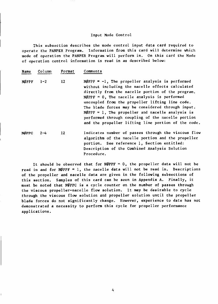
Input Mode Control
I This subsection describes the mode control input data card required to operate the PANPER Program. Information from this card will determine which mode of operation the PANPER Program will perform in. On this card the Mode of operation control information is read in as described below:
I Name Column Format Comments - NQPPF 1-2 I2 N$PPF = -1, The propeller analysis is performed
without including the nacelle effects calculated directly from the nacelle portion of the program. NQPPF = 0, The nacelle analysis is performed uncoupled from the propeller lifting line code. The blade forces may be considered through input. NQPPF = 1, The propeller and nacelle analysis is performed through coupling of the nacelle portion and the propeller lifting line portion of the code.
I NQPPC 2-4 I2 Indicates number of passes through the viscous flow algorithm of the nacelle portion and the propeller portion. See reference 1, Section entitled: Description of the Combined Analysis Solution Procedure.
It should be observed that for NQPPF = 0, the propeller data will not be read in and for NaPPF = 1, the nacelle data will not be read in. Descriptions of the propeller and nacelle data are given in the following subsections of this section. Samples of this card can be seen in Appendix A. Finally, it must be noted that N$PPC is a cycle counter on the number of passes through the viscous propeller-nacelle flow solution. through the viscous flow solution and propeller solution until the propeller blade forces do not significantly change. However, experience to date has not demonstrated a necessity to perform this cycle for propeller performance applications.
It may be desirable to cycle
4

P r o p e l l e r Po r t ion
Maior InDut Fea tu res
The major input f e a t u r e s c o n s i s t of four b a s i c groups of input d a t a a long wi th the a p p r o p r i a t e program c o n t r o l da t a . These four groups of d a t a are b lade geometry, a i r f o i l c h a r a c t e r i s t i c s , inf low p r o p e r t i e s and the wake geometry. i n some d e t a i l so t h a t t he user w i l l understand t h e i r importance.
I n the fol lowing subsec t ions , t hese groups of input are descr ibed
Blade L i f t i n g Line Geometry ------------- The geometr ic d e s c r i p t i o n of t he b lade l i f t i n g l i n e r e p r e s e n t a t i o n of t h e
b l ade is of primary importance f o r ob ta in ing the most accu ra t e s o l u t i o n s given t h e assumptions inherent i n the a n a l y s i s . The hub-pitch a x i s centered Car t e s i an coord ina te s fo r each l i f t i n g l i n e segment boundary must be input (XSB, YSB, ZSB) c o n s i s t e n t with the input blade t w i s t d i s t r i b u t i o n (THET) so t h a t the program can c o r r e c t l y r o t a t e t h i s geometry about the p i t c h axis f o r the r equ i r ed b lade angle . f o r t he t i p Mach cone c a l c u l a t i o n s (XMC, YMC, ZMC) must a l s o be input c o n s i s t e n t wi th the t w i s t d i s t r i b u t i o n . For counter r o t a t i n g c o a x i a l p r o p e l l e r s , each set of coord ina te s is input re ferenced t o i t s r e s p e c t i v e hub and p i t c h axis c e n t e r s . i s d e t a i l e d i n r e fe rence 1, see f i g u r e 2 . The s e l e c t i o n of t h e b lade segmentat ion i s of primary importance i n reg ions of severe loading g r a d i e n t s . For t h e s e reg ions ( g e n e r a l l y t h e t i p of the b lade) f i n e r segmentation i s r equ i r ed as compared with r eg ions of weak g rad ien t s .
The coord ina te s f o r the d e f i n i t i o n of the b lade t i p
The t e c h n i c a l d e s c r i p t i o n of t h i s coord ina te system
P r o p e l l e r Blade A i r f o i l C h a r a c t e r i s t i c s .................... To c a l c u l a t e t he b lade a i r l o a d i n g , i t is necessary t o s p e c i f y t h e
d i s t r i b u t i o n of a i r f o i l type along t h e b lade r a d i u s . There are three d i f f e r e n t sets of a i r f o i l d a t a a v a i l a b l e i n t h i s a n a l y s i s : two sets of NACA 16 series i s o l a t e d a i r f o i l d a t a , whose c h a r a c t e r i s t i c s are desc r ibed i n r e f e r e n c e 1, and one cascade a i r f o i l d a t a set f o r NACA 65 series, a l so descr ibed i n t h e above noted r e fe rence . The user s p e c i f i e s t h e use of t hese a i r f o i l d a t a sets by spec i fy ing the r a d i a l l o c a t i o n which denotes the o u t e r boundary of t he reg ion (RADCAS) f o r which i t is d e s i r e d t o use the cascade d a t a set . Outboard of t h i s reg ion , t he d i s t r i b u t i o n of t he i d e n t i f i c a t i o n number (23 o r 24) f o r the i s o l a t e d a i r f o i l d a t a sets is input through the a i r f o i l type des igna t ion number d i s t r i b u t i o n input (AIRN). p o s s i b l e to model t he cascade e f f e c t s on the i s o l a t e d a i r f o i l d a t a by a p p l i c a t i o n of an a n a l y t i c a l cascade c o r r e c t i o n (CASCAD). desc r ibed i n r e fe rence 1. The use of t h i s model may be d e s i r a b l e f o r two
I f d e s i r e d , i t i s
Th i s model is a l s o
5

reasons: first, if the inboard section of the propeller blades is not adequately modeled with NACA 65 series airfoil sections, and second, if the cascade influence extends beyond the region where the NACA 65 series airfoil types apply.
Once the distribution of airfoil type and cascade regions are- determined for the design under consideration, the particular airfoil characteristics are defined by additional input. These characteristics are: the design lift coefficient (DECL) , the thickness to chord ratio (TQVC), and the chord (CQRD).
Inflow ProEerties at the Blade Row ----- ----------- This analysis allows the user the ability to describe the noninduced
inflow properties at the propeller blade rows if run independent from the nacelle portion of the analysis. It is therefore possible to prescribe the nacelle's influence (or any desired influence) on the inflow conditions at the propeller blades without running the nacelle portion of the analysis. This may be desirable if the variation of the nacelle's influence is small for slight changes in the propeller designs. The inflow properties are the axial (VQVO) and radial (URVO) noninduced inflow velocity ratio distributions, and the density (DENS) and speed of sound (SQUN) ratio distributions along the blade radius. These distributions scale the respective freestream values to define the local inflow conditions at the blade rows.
Wake Model Description ----------- The description of an accurate wake geometry for the flight condition
under investigation is of primary importance for accurate predictions of the induced inflow solution and the resulting propeller blade air loading. The wake models available have been described in detail in the technical section of reference 1; however, a brief review of the applicable wake models for the different flight regions follows.
For static thrust conditions, the generalized wake model should be used (figure 3 ) . It has been clearly demonstrated to be the most accurate model available and is necessary for accurate performance solutions. Wake rollup modeling must also be used for this flight condition (figure 4). flight conditions, the classical (figure 3 ) or modified classical wake model (standard model for high speed flights) is probably sufficient for reasonable performance predictions; however, it is clear that the wake model must have some of the features of the generalized wake model (radial contraction, in particular). Because of this, it is possible to use the generalized wake model for nonzero flight speed conditions. In this case the generalized wake model will have the inflow velocity distribution superimposed on it to describe the wake geometry. Thus, with careful selection of the input gener- alized wake coefficients, it is possible to model a low speed wake geometry if
In low speed
6

the required characteristics are known. Wake rollup modeling should probably be used for these flight conditions. For high speed flight conditions, the wake is carried away from the propeller so rapidly that it is doubtful that any model other than the classical or modified classical wake will be required. Generally no wake rollup modeling is required at these flight speeds.
Similar considerations must be given to the influence of the nacelle on the wake geometry. For static thrust conditions, the nacelle influence cannot be modeled by using the nacelle portion of the analysis. displacement of the wake due to the presence of the nacelle is known, it can be modeled through the wake geometry input option. For all other flight con- ditions, the nacelle's influence can be included directly in the analysis.
However, if the
If it is desired for any reason to use a wake model which is not geomet- rically compatible with the basic wake models available, the wake geometry can be input in cylindrical coordinate form. This allows for a wide range of possible wake modeling capabilities in this analysis.
7

Deta i l ed Desc r ip t ion of P r o p e l l e r Data Input and Setup
Standard Input Data and SetuE -------------- The p r o p e l l e r input d a t a is grouped i n t o 3 d i s t i n c t d a t a sets, the f i r s t
set c o n s i s t s of input d a t a which desc r ibes the p r o p e l l e r a n a l y s i s 'modeling op t ions , f r ees t r eam f l i g h t cond i t ions and primary p r o p e l l e r c h a r a c t e r i s t i c s . The second set of d a t a d e f i n e s the phys ica l l o c a t i o n of the blade l i f t i n g l i n e segment boundaries and the coord ina t ion used t o d e f i n e the l o c a t i o n of t he t i p Mach cone. These items are re ferenced t o t h e i r r e s p e c t i v e c e n t e r s of ro ta - t i o n . The t h i r d set of d a t a is used t o d e s c r i b e the l o c a l b lade element f l i g h t inf low p r o p e r t i e s (based on the f r ees t r eam f l i g h t cond i t ion ) and secondary b lade c h a r a c t e r i s t i c s . Th i s d a t a set c o n s i s t s of i n t e r p o l a t i o n t a b l e s f o r t he r equ i r ed items. A l l of t hese input d a t a sets are descr ibed i n t h e fol lowing subsec t ions . For coax ia l p r o p e l l e r s , the second and t h i r d d a t a sets are repea ted f o r t he second p r o p e l l e r fol lowing a l l of t he d a t a sets f o r t h e f i r s t p r o p e l l e r . Two s a m p l e p r o p e l l e r input d a t a decks are l i s t e d i n Appendix A ( case 1 and case 3 ) f o r an i s o l a t e d p r o p e l l e r mode and a combined c o a x i a l p rope l l e r -nace l l e mode. Each d a t a set is i n i t i a t e d by a header ca rd wi th an alphanumeric l a b e l i n card columns 1 through 6 ( l e f t j u s t i f i e d ) and terminated by a card wi th the alphanumeric l a b e l END i n card columns 1 through
items and i f d u p l i c i t y of t h e i t e m occurs , t he l a s t va lue read w i l l be used. A l l numbers are input i n FORTRAN f l o a t i n g point or exponent ia l format.
I 3. Within a given d a t a se t , t h e r e is no o rde r ing dependency f o r the input
Data S e t I ----- The header card f o r t h i s d a t a set c o n s i s t s of t he c h a r a c t e r s INPUT i n
ca rd columns 1 through 5 . The input d a t a requi red f o r t h i s d a t a set is input one card at a t i m e fo l lowing t h e header card . Each card has a l a b e l and v a l u e punched on i t . The l a b e l des igna te s the i t e m and t h e va lue f o r t h a t i t e m fo l lows the l a b e l on t h e ca rd . The l a b e l is an alphanumeric, t h r e e t o six c h a r a c t e r name, l e f t j u s t i f i e d i n card columns 1 through 6 , with the input va lue fo l lowing i n a FORTRAN E20.8 format (columns 7 through 26) . The d e s c r i p t i o n of t he l a b e l s and corresponding input d a t a items are l i s t e d below. For items wi th the numeric c h a r a c t e r s 1 or 2 on t h e end of t h e l a b e l , the 1 and 2 des igna te the f i r s t and second p r o p e l l e r q u a n t i t i e s r e s p e c t i v e l y f o r a c o a x i a l cond i t ion . I f t he input i t e m is omi t ted , a va lue of 0.0 is used i n t e r n a l l y .
Input Label D e s c r i p t i o n
BLADE1 ,BLADE2
I Blade number per p r o p e l l e r
I C A S 0 Option switch t o use an a n a l y t i c a l cascade cor rec- t i o n on i s o l a t e d a i r f o i l d a t a , a v a l u e of 1.0 r eques t s t he model based on f l a t p l a t e theory , a v a l u e of 2 .0 uses a model based on empi r i ca l c o r r e l a t i o n s of r e fe rence 44 i n Volume I.
8

Input Label
CBWAKE
CNSECT
CgFLdW
CflMPRS
cpr
CTI
DCPDT
Description
Option control for including the effects of compres- sibility on the induced velocity calculation from the bound lifting line vortex (this model is of questionable validity). A value of 1.0 sets this option, a value of 2.0 sets this option but the bound influence on the blade generating the effect is neglected. Should use 0.0.
Fraction of the chord measured from the leading edge, used to determine the tip Mach cone inter- section location on the blade for the Evvard tip correct ion, generally the trailing edge (1 .O> is used. A zero input sets this value to 1.0.
Option control for overriding the limitation that the wake and bound vortex compressibility effects be applied only when the section Mach numbers are greater than 1.0. (This model is of questionable validity.) An input value of 1.0 engages this option. Should use 0.0, see section entitled: Compressibility Considerations for Induced Velocity, of reference 1.
Option control for including the effects of compres- sibility on the induced velocity calculation from the trailing wake geometry. A value of 1.0 sets this option. This option should be used.
Requested power coefficient for performance iter- ation. A zero value assumes no iteration. This iteration option will not work for coaxial pro- pellers.
Requested thrust coefficient for performance itera- tion. A zero value assumes no iteration. This iteration option will not work for coaxial propel- lers. The power iteration will override this option if both are requested.
The derivative of power coefficient with respect to blade angle. If the power coefficient iteration is requested and this value is nonzero, the input value is used to determine the second iteration blade angle value, otherwise a change of 1.5 degrees in blade angle is used for the second iteration.
9

DescriDtion Input Label
DCTDT
DEBUG
DENSTY
DFRNAC
DPRNAC
DPSI
I EVAARD
The derivative of thrust coefficient with respect to blade angle. If the thrust coefficient iteration is requested and this value is nonzero, the input value is used to determine the second iteration blade angle value, otherwise a change of 1.5 degrees in blade angle is used for the second iteration.
Intermediate print option control, generally not used (0.0). A value of 1.0 requests printout of many quantities associated with the geometry trans- formations, geometric influence coefficients, circu- lation matrix and intermediate aerodynamic quantities. A value of 2.0 requests a full debug printout and should not be used.
Freestream air density (slugs/ft 3 ,
Input skin friction drag (lbf) due to the nacelle. Included in the performance calculation if input A positive value is opposite the direction of positive thrust.
Input pressure drag (lbf) due to the nacelle. Included in the performance calculation if input. A positive value is opposite the direction of positive thrust.
Maximum size of the azimuth increment (degrees) allowed to define the wake geometry and azimuthal interval in either single or coaxial mode. The program internally calculates the actual value.
Option switch to request tip relief model. An input value of 1.0 requests tabled values for the Evvard model be used, a value of 2.0 requests that a func- tional form for the Evvard model be used which is slightly different than the tabled values, a value of 3.0 requests that conical flow theory be used with a variable Mach number distribution, while a value of 4.0 uses a fixed Mach number.
Option switch to couple via an external file to an aeroelastic response analysis. If nonzero, the value identifies the device unit number t o be used.
10

Description Input Label
HUBQ1, HUBQ2
PRINT1
PRMAT
P RNTgP
PRgPT
PRQPNM
RAD1, RAD2
RDCAS1, RDCAS2
RDTRNl, RDTRN2
REV
Input hub torque (ft-lbf). be included in the performance calculations and performance iteration loops. A positive value represents a power loss which the engine must over- come. However, the fluid does not sense this loss.
This input value will
Option to delete vector input listing, nonzero to perform this function.
Geometric Influence Coefficient print option, generally not used (0.0). A value of 1.0 requests the printout of the geometric influence coefficients used to compute the induced velocity in both the cylindrical coordinate system and the blade element coordinate system.
Option to delete performance printout of spanwise distribution quantities, nonzero to perform this f unc t ion.
Wake geometry print option, generally not used (0.0). A value of 1.0 requests that the wake coordinates be printed.
Number of propeller blade rows (1 or 2 ) .
Input blade radius (along the pitch axis), this value may not be the true radius if the blade is swept off of the pitch axis (ft).
Outermost fraction of the blade radius for which the cascade airfoil data will be applied. If zero no cascade airfoil data is used.
Maximum radius to which the airfoil transition interpolation model can be applied. also the flag which requests this option.
This value is
Number of revolutions of wake geometry used to model the actual wake. The value chosen should be sufficient in length to approximately model an infinite wake's influence. Low flight speeds require a larger number of revolutions of wake geometry than high speed conditions. For high speed conditions use 2.0.
11

InDut Label Descr iDtion
R0 LUP 1, RQ LUP2
RPMRFI, RPMRF2
RPMl, RPM2
I SKINflP
SQUND I
I
I STACK
STN ,
TAUEXP
THETA 1, THETA2
Option switch t o model t r a i l i n g wake r o l l u p . A nonzero value r eques t s t h a t the input va lue repre- s e n t s the number of ou te r f i l amen t s t o be r o l l e d up i n t o the t i p vo r t ex f i lament at a specif . ied azimuth p o s i t i o n behind the b lade . When t h i s model is reques ted , t he remaining f i l amen t s are i m p l i c i t l y r o l l e d up i n t o a remaining or root vor tex . See f i g u r e 4. The va lue t o use should correspond t o the maximum c i r c u l a t i o n l o c a t i o n .
Reference rpm f o r t w i s t increment due t o s t eady a i r loads .
P r o p e l l e r r o t a t i o n speed (rpm).
Option switch which r eques t s a skewed flow drag model. An input va lue of 1.0 r eques t s t h i s op t ion .
Freestream speed of sound ( f p s ) .
F r a c t i o n of chord measured from t h e lead ing edge t o d e f i n e the p o s i t i o n of t he l i f t i n g l i n e on each b lade element, g e n e r a l l y the q u a r t e r chord l i n e i s used (0.25) .
Number of inf low s t a t i o n s per b lade . Maximum of 15. Genera l ly at least 10 are used.
Exponent f o r a i r f o i l t r a n s i t i o n i n t e r p o l a t i o n func t ion .
Input r e fe rence b lade angle (deg rees ) . This r e f e r - ence angle r o t a t e s t he input t w i s t d i s t r i b u t i o n about t h e p i t c h a x i s . I f t he performance i t e r a t i o n i s reques ted t h i s va lue w i l l be changed i n t e r n a l l y and the input va lue is the f i r s t i t e r a t i o n value. P o s i t i v e lead ing edge up.
12

Description Input Label
TRUCI 1, TRUCI2
TRUCTl, TRUCT2
TYPCAS
VIMgM1, VLMdM2
VKTAS
V@RC@R
WAKEgP
WAKNAC
Azimuth position behind the blades for which the root rollup occurs, a zero value assumes rollup starts immediately at the blade. Because there is generally no root vortex formed, a large-value should be input when rollup is requested (degrees).
Azimuth position behind the blades for which the tip rollup occurs, a zero input assumes rollup starts immediately at the blades (degrees).
Option switch to select cascade type, An input of 0.0 requests no cascade data be used. A value of 1.0 uses the correlation from reference - , while a value of 2.0 requests the correlation of reference
Input momentum induced velocity, used to define the wake geometry. If a performance iteration is requested, this value is internally corrected to match the resultant performance (fps).
Freestream flight velocity (knots).
Fraction of the blade radius to define a vortex core for geometric influence coefficient calculations. Generally 10 percent of the chord is used.
Option control for wake model selection. A zero value requests the standard wake model (modified '
classical wake) defined by the momentum-induced velocity and the radially varying input axial inflow velocity distribution be used. A value of 1.0 requests a wake model defined by the flight velocity and momentum input velocity be used (classical wake). A value of 2.0 requests that the wake geometry be input to the analysis and a value of 3.0 requests that the wake coefficients for the general- ized wake model be input.
Option control for including the effects of the nacelle on the wake geometry through the use of a displacement correction to the requested wake model. The option generally requires that WAKEQP that double accounting of the nacelle's influence on the wake geometry does not occur. An input value of
1.0 so
1 3

Input Label Desc r ip t ion
1.0 r eques t s t h i s op t ion . I f the s tandard wake model (WAKEgP = 0.0) is reques ted with t h i s op t ion , the program execut ion w i l l be terminated- because of t h i s double account ing of t he n a c e l l e ' s in f luence . I f it is a c t u a l l y des i r ed t o use the s tandard wake model, t h i s f e a t u r e can be over r idden by adding t o the program inpu t , immediately fol lowing the input d a t a , a card with the alphanumeric c h a r a c t e r s OVER i n card columns 1 t o 4 .
ZHUB Nondimensional ( r a d i u s of p r o p e l l e r one) d i sp l ace - ment between the p r o p e l l e r d i s c c e n t e r s f o r coax ia l p r o p e l l e r s . A p o s i t i v e va lue p l aces the second p r o p e l l e r behind the f i r s t . Must be c o n s i s t e n t with input f o r n a c e l l e p o r t i o n of the a n a l y s i s .
Data Se t I1 ------ The header card l a b e l f o r t h i s d a t a set i s BLADE, i n card columns 1
through 5 . The f i r s t input a f t e r t h e header card must be the i n t e g e r va lue for t he number of b l ade segment boundaries , f r e e f i e l d format. Following t h i s input ca rd , t h e d a t a i t e m s are inpu t . For each set of blade segment boundary items (STN+l), a l abe led header card is input wi th the alphanumeric l a b e l s desc r ibed below, followed by the f r e e f i e l d formatted vec to r ( r o o t t o t i p ) on the next card f o r t he item i n ques t ion . For the t i p Mach cone d e f i n i t i o n q u a n t i t i e s , t h i s format is i d e n t i c a l but t he vec to r i t e m is rep laced by a s i n g l e va lue . A l l of t h e s e items should be inpu t .
*
Inpu t Label D e s c r i p t i o n
XSB
YSB
Input Car t e s i an coord ina te v e c t o r , X, inboard t o outboard, t o d e f i n e t h e b lade l i f t i n g l i n e segment boundaries . r a d i u s boundary va lue (RAD1). Maximum of 16 boundaries (15 segments).
Nondimensionalized by t h e b lade segment
Input Car t e s i an coord ina te , Y, t o d e f i n e the b l ade l i f t i n g l i n e segment boundaries , nondimensionalized by the l as t segment boundary va lue (RAD1). Maximum of 16 boundaries (15 segments).
* Free f i e l d format c o n s i s t s of a series of numbers ( F o r t r a n f l o a t i n g poin t or exponen t i a l ) s epa ra t ed by c o m a s . I f mre than 80 card columns are needed f o r an input v e c t o r , t he v e c t o r cont inues on the fol lowing card .
14
Input Label D e s c r i p t i o n
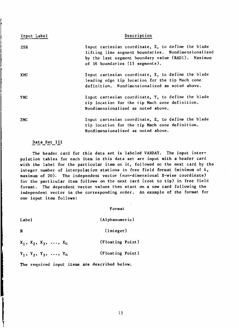
ZSB
XMC
YMC
ZMC
Input C a r t e s i a n coord ina te , Z , t o d e f i n e t h e b lade l i f t i n g l i n e segment boundaries . Nondimensionalized by t h e l a s t segment boundary va lue (RADl). Maximum of 16 boundaries (15 segments).
Input C a r t e s i a n coord ina te , X, t o d e f i n e the b lade leading edge t i p l o c a t i o n f o r t h e t i p Mach cone d e f i n i t i o n . Nondimensionalized as noted above.
Input C a r t e s i a n coord ina te , Y , t o d e f i n e the b lade t i p l o c a t i o n fo r t he t i p Mach cone d e f i n i t i o n . Nondimens i o n a l ized as noted above.
Input C a r t e s i a n coord ina te , Z , t o d e f i n e the b lade t i p l o c a t i o n fo r t he t i p Mach cone d e f i n i t i o n . Nondimensionalized as noted above.
Data Se t 111 ------ The header card f o r t h i s d a t a set is labe led VARDAT. The input i n t e r -
p o l a t i o n t a b l e s f o r each i t e m i n t h i s d a t a set a r e input with a header card with t h e l a b e l f o r t h e p a r t i c u l a r i t e m on i t , followed on the next card by t h e i n t e g e r number of i n t e r p o l a t i o n s t a t i o n s i n f r e e f i e l d format (minimum of 4 , maximum of 20). The independent v e c t o r (non-dimensional X - w i s e c o o r d i n a t e ) f o r t h e p a r t i c u l a r i t e m fol lows on t h e next card ( r o o t t o t i p ) i n f r e e f i e l d format. The dependent v e c t o r va lues then s ta r t on a new card fol lowing t h e independent v e c t o r i n t h e corresponding o rde r . An example of t he format f o r one input item fol lows:
Format
Label (Alphanumeric)
N ( I n t e g e r )
The requi red input items are descr ibed below.
I I
15

Input Label
AIRN
CQRD
THET
DECL
TgVC
DENS
SQUN
URVO
vevo
BETA
Description
Airfoil type designation number distribution. There are only two values for input, 23.0 which requests the Manoni airfoil data tables and 24.0 which requests the NACA airfoil data tables (reference 1). Because the values used internally are computed by interpolation from this input vector and then converted to integer values, the input values of 23.1 and 24.1 are generally used to guarantee that the integer values of 23 and 24 are used internally. These values start at the hub even if the cascade data is used.
Chord distribution in feet.
Built in blade twist distribution in degrees. Leading edge up (direction of positive rotation) is positive.
Design lift coefficient distribution.
Airfoil thickness to chord ratio distribution.
Local blade row density to freestream density ratio distribution. Overridden if Nacelle portion of the analysis is used.
Local blade row to freestream speed of sound ratio distribution. Overridden if Nacelle portion of the analysis is used.
Local blade row radial inflow velocity to freestream velocity ratio distribution. portion of the analysis is used.
Overridden if Nacelle
Local blade row axial inflow velocity to freestream velocity ratio distribution. Overridden if Nacelle portion of the analysis is used.
Dynamic twist distribution, internally scaled by the ratio of rpm to reference rpm squared. Incremen- tally added to static twist distribution, degrees.
16
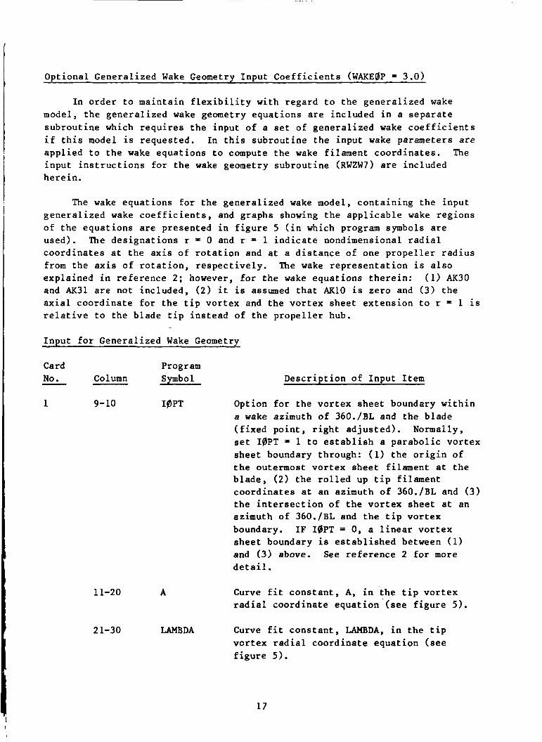
Optional Generalized Wake Geometry Input Coefficients (WAKEgP = 3.0)
In order to maintain flexibility with regard to the generalized wake model, the generalized wake geometry equations are included in a separate subroutine which requires the input of a set of generalized wake coefficients if this model is requested. In this subroutine the input wake parameters are applied to the wake equations to compute the wake filament coordinates. The input instructions for the wake geometry subroutine (RWZW7) are included herein.
The wake equations for the generalized wake model, containing the input generalized wake coefficients, and graphs showing the applicable wake regions of the equations are presented in figure 5 (in which program symbols are used). The designations r = 0 and r = 1 indicate nondimensional radial coordinates at the axis of rotation and at a distance of one propeller radius from the axis of rotation, respectively. The wake representation is also explained in reference 2; however, for the wake equations therein: (1) AK30 and AK31 are not included, ( 2 ) it is assumed that AKlO is zero and (3) the axial coordinate for the tip vortex and the vortex sheet extension to r = 1 is relative to the blade tip instead of the propeller hub.
Input for Generalized Wake Geometry
Card Program No. Column Symbol Description of Input Item
1 9- 10 IPPT Option for the vortex sheet boundary within
-
a wake azimuth of 360./BL and the blade (fixed point, right adjusted). Normally, set 10PT = 1 to establish a parabolic vortex sheet boundary through: (1) the origin of the outermost vortex sheet filament at the blade, (2 ) the rolled up tip filament coordinates at an azimuth of 360./BL and (3) the intersection of the vortex sheet at an azimuth of 360./BL and the tip vortex boundary. IF IQPT = 0, a linear vortex sheet boundary is established between (1 and (3) above. See reference 2 for more detail.
11-20 A
2 1-30 LAMBDA
Curve fit constant, A, in the tip vortex radial coordinate equation ' (see figure 5
Curve fit constant, LAMBDA, in the tip vortex radial coordinate equation (see figure 5 ) .
17

Card Program No. Co 1 umn Symbol Desc r ip t ion of Input Item -
3 1-40 PHINPO Wake aximuth angle , PHINPO, t h a t s e p a r a t e s t h e a x i a l v e l o c i t y reg ions AK20 and AK30 for the vo r t ex shee t ex tens ion t o r = 0 , degrees ( s e e f i g u r e 5 ) .
41-50 PHINPl Wake azimuth ang le , PHINP1, t h a t s e p a r a t e s t he a x i a l v e l o c i t y reg ions AK21 and AK31 for the vo r t ex shee t ex tens ion r = 1, degrees ( s e e f i g u r e 5 ) .
2 1-10 AKlT Axial v e l o c i t y of the t i p vo r t ex between
blade a t wake azimuth 360./BL (nondimen- s i o n a l i z e d by r o t o r t i p speed; nega t ive down).
I t h e blade and the passage of t he following ~
11-20 AK2 T
2 1-30 AK 10
31-40 AK20
41-50 AK30
51-60 A K l l
Axial ve loc i ty of the t i p vortex a f t e r the passage of the following b lade a t t he wake azimuth 360./BL (nondimensionalized by r o t o r t i p speed; nega t ive down).
Axial v e l o c i t y of t he vo r t ex shee t ex tens ion t o t h e c e n t e r of r o t a t i o n i n the wake azimuth reg ion between the b lade and t h e passage of t he following b lade a t t he wake azimuth 360./BL (nondimensionalized by r o t o r t i p speed; nega t ive down).
Axial v e l o c i t y of the v o r t e x shee t exten- s i o n t o the c e n t e r of r o t a t i o n i n t h e wake azimuth r eg ion between the passage of t h e fo l lowing b lade a t t h e wake azimuth 360./BL and t h e wake azimuth PHINPO (nondimension- a l i z e d by t i p speed; nega t ive down).
Axial v e l o c i t y of the vo r t ex shee t ex tens ion t o t h e c e n t e r of r o t a t i o n following the wake azimuth PHINPO (nondimensionalized by t i p speed; nega t ive down).
Axial v e l o c i t y of t he vo r t ex shee t ex tens ion t o r = 1 i n the wake azimuth r eg ion between t h e b lade and the passage of t he fo l lowing b l ade at t h e wake azimuth 360./BL (nondimen- s i o n a l i z e d by r o t o r t i p speed; nega t ive down).
18

Card Program No. Co 1 umn Symbol Descripti n of Input Item
61-70 AK2 1 Axial velocity of the vortex sheet extension to r = 1 in the wake azimuth region between the passage of the following blade at the wake azimuth 360./BL and the wake azimuth PHINPl (nondimensionalized by tip speed; negative down).
7 1-80 AK3 1 Axial velocity of the vortex sheet extension to r = 1 following the wake azimuth PHINPl (nondimensionalized by tip speed; negative down).
Optional Input Wake Geometry (WAKE0P = 2.0)
If desired, an arbitrary wake geometry model may be used in the analysis by input of the complete wake geometry. model are that the description of the geometry is assumed identical for each blade (a required assumption in the solution procedure) and that the coordinates be input in the cylindrical coordinate system for equally spaced wake azimuth positions consistent with the blade azimuth increment and inflow station boundaries. .This model allows for the most exact description of the wake geometry, if known, given the inherent assumptions of the analysis. The description of the input format follows.
The only constraints for the wake
The wake geometry is input in separate sets for each trailing wake fila-
Each subset will start with a new card. The radial ment, inboard to outboard. Each set contains subsets for each revolution of wake geometry requested. and axial coordinates are paired (radial, axial) for the trailing wake segment boundary for each wake azimuth position (wake age) starting at the youngest and ending with the oldest wake segment boundary. position is implicitly assumed to be consistent with the input blade azimuth (DPSI) increment and the number of trailing segments must be constant with the number of wake revolutions. The FORTRAN format used is 10F8.4 for each card of data. There are KTflT (number of trailing filament) sets of cards. Each set of cards contains NTflT (number of wake revolutions) subsets, with each subset containing JTflT1 (number of wake azimuth positions per revolution + 1) pairs of wake coordinates. complete definition of a revolution of wake geometry, the first coordinate pair of each subset will be identical to the last coordinate pair of the previous revolution, excepting the first subset. The total number of input data pairs is then (KTflT)x(NT@T)x(JTflTl). using two revolutions of wake, 12 segment boundaries and a blade azimuth increment of 15 degrees, the number of pairs would be (12)x(2)x(25) = 600 or 1200 single values.
Thus, the wake azimuth
Because each subset of data will contain a
For a typical high speed condition
19

Description of Propeller Solution Output
The propeller output section can be broken into three distinct portions, initial, intermediate and final output. The program user has a large number of print options which control the amount of intermediate output. The initial and final output are not optional. The descriptions of the output quantities are presented in the following sections. A sample printout for selected por- tions of the propeller solution portion is presented in Appendix B. It should be noted that in the description to follow there is only one propeller and propeller position for a single propeller configuration. propellers the intermediate output is repeated for each propeller.
For coaxial
Initial Output ------- During the reading of the propeller input data, the data as read in is
immediately printed out. This information is entitled: PRINTOUT OF INITIAL DATA AS READ IN, and if the program execution terminates during the reading of an input data item, the user will see the item which was last read before program termination. This feature has two advantages: first, if an incorrect item is attempted to be read in, the user can quickly determine the incorrect item; and second, a complete listing of the propeller input data as used in the analysis is available for later review if desired. This output section always occurs during the input of the propeller data. analysis (propeller and nacelle) mode is being used, this output occurs long before (precedes the nacelle inviscid solution) the other portions of the propeller output. This feature can be partially suppressed if desired by the input control, PRINTI. This option will suppress the vector printout quantities if requested.
If the combined
I The next output for this initial output is a section entitled: PROGRAM INPUT SUMMARY, and consists of the input data displayed in a structured format. The propeller modeling options used for the particular execution are listed in the following form. The integer value of the input modeling option is displayed with a brief description of the model used. conditions are listed next, (VKTAS, SBUND, DENSTY) followed by the propeller operating characteristics (PRBPNM, BLADEN, RF’M, ZHUB). The parameters which define the wake and blade geometry segmentation are displayed next (STN, STACK, DPSI, REV, CNSECT) followed by the propeller characteristics (RAD1, HUBQ1, THETAl, RDCAS1, VIMBMl) of each propeller. propeller characteristics includes: the blade lifting line segment boundaries coordinates (XSB, YSB, ZSB, BETA); the inflow station coordinates and the blade properties at the segment centers as interpolated from the input distri- butions (AIRN, CQRD, THET, DECL, TBVC, V0V0, URVO, SBUN, DENS).
The freestream
The printout of the
20

Intermediate ------ The intermediate output is described below. Generally it is limited to
the minimum amount possible since most of the output is repeated in the final output section. The intermediate output is repeated for each iteration in blade angle. If there is no performance iteration it is printed only once for the input blade angle. This output is entitled: PROGRAM OUTPUT FOR PROPELLER PERFORMANCE ITERATION "MBER X.
The first output data for this section is not optional; it consists of a table of the blade lifting line segment center and boundary coordinates for the reference blade angle and the blade angle value in degrees. nates are listed in Cartesian and cylindrical form for the centers and bound- aries. Following this table, the coordinates for the definition of the tip Mach cone location are listed in Cartesian form for the blade angle in ques- tion. If no optional printouts are requested, the wake transport velocity distribution is printed as a function of blade radial location. If optional printouts are requested this print does not follow immediately, but occurs later in the output. All other output for the intermediate portion is optional. descriptions of the output follow (output labels in parentheses if not noted).
The coordi-
The input option controls (in parentheses) and the respective
The output of the trailing wake geometry coordinates (PRflPT) is presented in the cylindrical coordinate system and tabulated as a function of wake azimuth position and blade radial position. This output is entitled: WAKE COORDINATES. The radial coordinates are tabulated first, starting with the values at the blade and ending with the oldest element. coordinates is then presented in the same format.
A table of the axial
The printout (PRMAT) of the summed geometric influence coefficients for each inflow station at each propeller position for each propeller as a func- tion of the appropriate inflow station and propeller position of each propeller is presented in the cylindrical coordinate system and in the blade element coordinate system. This printout is entitled: CYLINDRICAL GEOMETRIC INFLUENCE COEFFICIENTS or BLADE ELEMENT GEOMETRIC INFLUENCE COEFFICIENTS. The propeller and propeller position indices are so noted on the printout, while the inflow station indices are not, since the values are presented for the inboard station to the outboard station for each propeller and propeller posit ion.
For detailed intermediate output (DEBUG) the following extensive list of items is presented in the same format as noted above for the propeller, pro- peller position and inflow station indices. not be used. A section of detailed blade element properties consisting of the magnitude (if it applies) and unit vector direction cosines in the cylindrical coordinate system is output for each of the following:
Generally this printout should
the blade segment
21

l i f t i n g (SB, ALSRAD, ALSPHI, ALSAXL), input chord (CINPUT, ALCIRD, ALCIPH, ALCIAX), the normalwise u n i t vec to r (ALNRAD, ALNPHI, ALNAXL), the blade element chord nondimensionalized by blade r ad ius (CHBRD, ALCRAD, ALCPHI, ALCAXL), input blade element t h i ckness t o chord r a t i o (TQVERC, ALTIRD, ALTIPH, ALTIAX), t he b lade element t h i ckness t o chord r a t i o magnitude only (THK) and the blade element des ign l i f t c o e f f i c i e n t (DESCLP). This s e c t i o n i s e n t i t l e d : DETAILED BLADE ELEMENT OUPUT. The next s e c t i o n c o n s i s t s of d e t a i l e d b lade element v e l o c i t i e s and u n i t vec to r d i r e c t i o n cos ines (VTgT, ALVRAD, ALVPHI, ALVAXL) i n the c y l i n d r i c a l coord ina te system along with the d i r e c t i o n cos ines i n the blade element coord ina te system (VS, VC, VN) and the angle of a t t a c k (ALPHAN), and inp lane aerodynamic skew angle (SKEW), a l l computed without inc luding the p r o p e l l e r induced v e l o c i t i e s , e n t i t l e d : DETAILED VELOCITY RELATED OUTPUT (EXCLUDING INDUCED VELOCITY TERMS). The ind ices a s soc ia t ed with t h e i n t e r n a l program "DO LOOPS" f o r t he geometric i n f luence c a l c u l a t i o n s a r e then ou tpu t , a long with the cos ine and s i n e func t ions f o r the r e s p e c t i v e inf low s t a t i o n s inp lane l a g angle and p r o p e l l e r azimuth p o s i t i o n and a coun te r r o t a t i o n f l a g with each l i n e of output marked: INTERMEDIATE OUTPUT. Following t h i s ou tpu t , t he normalwise blade element geometric i n f luence c o e f f i c i e n t s a r e p r i n t e d i n the c i r c u l a t i o n ma t r ix form f o r each p r o p e l l e r a t each p r o p e l l e r p o s i t i o n f o r each inf low s t a t i o n . The t i t l e of the output i s : GEOMETRIC INFLUENCE COEFFICIENT. Following t h i s output some u n t i t l e d cascade r e l a t e d items a r e l i s t e d . The chord-to-gap r a t i o s (TAU) and gap-to-chord r a t i o s (SIGMA) a r e l i s t e d along with the geometric angle between the p r o p e l l e r d i r e c t i o n of r o t a t i o n and the l o c a l blade element chordwise vec to r (THETAG) which r e p r e s e n t s t he compliment of t he cascade s t agge r angle . T ip Mach cone q u a n t i t i e s ( u n t i t l e d ) a r e then ou tpu t . The Mach cone angle is l i s t e d and then t h e angle between the b lade t i p and the l o c a t i o n of the s p e c i f i e d f r a c t i o n of t he b lade chord f o r each inf low s t a t i o n i s l i s t e d . The t i p Mach number va lue i s l i s t e d next . The s t a t i o n l o c a t i o n index (NSTAT) f o r t h e i n t e r s e c t i o n of t he Mach cone and the f r a c t i o n of the blade chord is l i s t e d and the r e s u l t i n g
f o r each b lade inf low s t a t i o n i s presented . (CMACH) d i s t r i b u t i o n s a r e l i s t e d along with the b lade element geometric angle of a t t a c k (exc luding induced terms) d i s t r i b u t i o n i n r ad ians (ALPHA). Following t h i s ou tpu t , t he l i n e a r i z e d l i f t curve s lope (AA), an aerodynamic
geometr ic b lade angle (THETA) i n degrees a r e l i s t e d .
a t each inf low s t a t i o n of each p r o p e l l e r f o r each p r o p e l l e r p o s i t i o n a r e presented due t o each p r o p e l l e r , followed by t h e t o t a l of both p r o p e l l e r s f o r each inf low s t a t i o n (VINT, VICT, VIST), e n t i t l e d : DETAILED INDUCED VELOCITY OUTPUT. This output i s followed by the t o t a l v e l o c i t y magnitude (VTBT), t he b l ade element angle of a t t a c k (ALPHA), t h e b lade element aerodynamic skew angle (SKEW) and b lade element in f low angle (PHI) d i s t r i b u t i o n s which inc lude the induced v e l o c i t i e s . It i s t i t l e d : DETAILED VELOCITY RELATED OUTPUT.
I Evaard Tip Re l i e f c o r r e c t i o n f a c t o r (XKCgNE) The b lade element Mach number (SMACH) and the t o t a l Mach number
8 R I q u a n t i t y
component d i s t r i b u t i o n s (VIN, V I C , VIS) i n t h e b lade element coord ina te system
(D = c), t he ma t r ix cdns t an t vec to r (CgNST) and the b lade element The induced v e l o c i t y
I
22

The above output s t a r t i n g from t h e Mach cone c o r r e c t i o n and ending with t h e inf low angle is repea ted f o r each i t e r a t i o n of t h e non l inea r c i r c u l a t i o n ma t r ix s o l u t i o n . The in t e rmed ia t e c i r c u l a t i o n s o l u t i o n output c o n s i s t s of t he non l inea r c o r r e c t i o n q u a n t i t i e s (CgRPHI, CgRVEL, CgRCL) used i n t h e s o l u t i o n technique , t he r e s u l t i n g c o r r e c t e d cons t an t v e c t o r of t h e c i r c u l a t i o n ma t r ix (CBNHSD), t h e a c t u a l c o r r e c t i o n v,ector (CFDP), t he uncorrec ted cops t an t v e c t o r (CBNST), t h e c u r r e n t angle of a t t a c k (ALPHA), and previous ang le of a t t a c k (SAVALP), t he c u r r e n t l i f t c o e f f i c i e n t (CLSAV), t he c u r r e n t c i r c u l a t i o n (CIRC) and previous c i r c u l a t i o n (SAVCIR), and the c u r r e n t normalwise induced v e l o c i t y (VIN) f o r each inf low s t a t i o n f o r each p r o p e l l e r p o s i t i o n of each p r o p e l l e r f o r each i t e r a t i o n of t he ma t r ix s o l u t i o n . Once t h e f i n a l c i r c u l a t i o n i t e r a t i o n s o l u t i o n is ob ta ined , t h e f i n a l l i f t , d rag and minimum drag c o e f f i - c i e n t s a r e p r i n t e d (CLSAV, CDSAV, 0). Following t h i s ou tput t he t o t a l b lade f o r c e s are l i s t e d i n terms of t h e magnitude and d i r e c t i o n cos ines (FTgT, ALFRAD, ALFPHI, ALFAXL) and the r e s p e c t i v e l i f t and drag components of the fo rce (FLTBT, ALFLRD, ALFLPH, ALFLAX, FDTBT, ALFDRD, ALFDPH, ALFDAX). This ou tpu t i s marked: DETAILED BLADE FORCE SUMMARY.
F i n a l Output ------ The f i n a l ou tput c o n s i s t s of t ab led va lues of many of t h e output items
l i s t e d i n t h e in t e rmed ia t e p r i n t o u t and i n t e g r a t e d performance q u a n t i t i e s . This ou tput s e c t i o n is e n t i t l e d : PROPELLER PERFORMANCE. It is repea ted f o r each performance i t e r a t i o n and presented f o r each p r o p e l l e r f o r each p r o p e l l e r p o s i t i o n a s a func t ion of b lade inf low s t a t i o n l o c a t i o n (X/R). The desc r ip - t i o n of each of t h e t a b u l a t e d i tems i s included on t h e p r i n t o u t of Appendix B and w i l l not be desc r ibed he re . It i s l abe led : BLADE SPANWISE VARYING QUANTITIES. Only t h e d e s c r i p t i o n s of t h e s e c t i o n s of i n t e g r a t e d q u a n t i t i e s w i l l be presented . The f i r s t o f t h e s e in.tegrated s e c t i o n s is l abe led BLADE CHARACTERISTICS and c o n t a i n s the b lade c h a r a c t e r i s t i c s f o r each p r o p e l l e r p o s i t i o n f o r each p r o p e l l e r ; t h r u s t per b lade ( l b f ) , to rque per b lade ( f t - l b f ) , power per b lade ( f t - l b f / s e c ) and horsepower per b l ade (hp). Following t h i s s e c t i o n of i n t e g r a t e d q u a n t i t i e s , t h e combined ( a l l b l a d e s , bo th p r o p e l l e r s ) i n s t an taneous va lues of t h r u s t and power f o r each p r o p e l l e r p o s i t i o n are presented . It is t i t l e d : INSTANTANEOUS TOTAL PROPELLER PERFOR- MANCE FOR PROPELLER POSITION X. This i s followed by a s e c t i o n of i n t e g r a t e d v a l u e s averaged over a l l p r o p e l l e r p o s i t i o n s f o r each p r o p e l l e r , e n t i t l e d : INTEGRATED PROPELLER CHARACTERISTICS FOR PROPELLER X. This s e c t i o n c o n t a i n s t h e t o t a l t h r u s t ( l b f ) , t h r u s t c o e f f i c i e n t (T/ n2D4), forward v e l o c i t y
23

(kno t s ) , to rque ( f t - l b f ) , power c o e f f i c i e n t (P/pn3D5), advance r a t i o (Vn /QR) , p r o f i l e torque ( f t - l b f ) , p r o p e l l e r e f f i c i e n c y (CTXJ/Cp) , r e fe rence b l a d e angle (deg rees ) , induced torque ( f t - l b f ) , power ( f t - l b f / s e c ) , horse- power (hp) and the momentum induced v e l o c i t y ( f p s ) . The combined p r o p e l l e r performance fol lows i f c o a x i a l p r o p e l l e r s are used. This ou tput i s followed by t h e n a c e l l e and combined nace l l e -p rope l l e r q u a n t i t i e s . These items f o r t h e n a c e l l e are the p re s su re and s k i n f r i c t i o n drag ( l b f ) , t h e r e s p e c t i v e drag c o e f f i c i e n t s and t h e combined drag and drag c o e f f i c i e n t s us ing the same u n i t s and d e f i n i t i o n s as used f o r t h e p r o p e l l e r s . The combined n a c e l l e and p r o p e l l e r t h r u s t , t h r u s t c o e f f i c i e n t , power and power c o e f f i c i e n t and e f f i c i e n c y then follow. Following t h i s ou tpu t , t h e force components per b l ade p e r u n i t span a r e presented i n t h e c y l i n d r i c a l coord ina te system ( l b f / f t ) f o r each p r o p e l l e r , and l abe led : FORCE PER BLADE PER U N I T SPAN.
D e s c r i p t i o n of F a i l u r e Modes
Genera l ly , i f t he input d a t a is c o r r e c t and reasonable f o r t he f l i g h t c o n d i t i o n be ing i n v e s t i g a t e d , t h e p r o p e l l e r s o l u t i o n procedure w i l l not f a i l . To h e l p ass is t t h e use r i n running the computer program, c e r t a i n f a i l u r e s which could occur because of incor rec t da t a s e t u p or i n c o r r e c t da t a va lues are checked i n t e r n a l l y by t h e computer program. I f t h e input i s i n c o r r e c t , d i a g n o s t i c ou tput w i l l occur t o inform the use r and a l low him t o make the r equ i r ed c o r r e c t i o n s .
General Input Format ---------- As noted i n t h e s e c t i o n d e s c r i b i n g the input d a t a se tup , c e r t a i n l a b e l -
l i n g formats have been s p e c i f i e d f o r t h e input da t a . I f t h e s e formats are v i o l a t e d , e x p l i c i t ou tput d i a g n o s t i c s w i l l not g e n e r a l l y be p r i n t e d ; however, program t e rmina t ion w i l l occur immediately with the l a s t i tem which was at tempted t o be read i n p r i n t e d as the l a s t ou tput . Terminat ion on t h e inpu t o f t h e s e l a b e l s w i l l occur f o r t h e fol lowing reasons :
(1 ) Data se t l a b e l s not i n t h e r equ i r ed o rde r ( 2 ) Data set l a b e l s mispunched ( 3 ) Input item l a b e l s mispunched (4) Missing END l a b e l s f o r t h e d a t a sets
Miss ing Input Data --- ----- Assuming a l l of t he input d a t a is read i n c o r r e c t l y , t h e program then
checks f o r miss ing input t h a t is r equ i r ed f o r s u c c e s s f u l program execut ion . The fol lowing d i a g n o s t i c messages could occur i f c e r t a i n d a t a is miss ing . Explana t ions of t h e messages are noted, i f r equ i r ed , f o r c l a r i t y .
24

( 1 ) "PROPELLER DISK DISPLACEMENT NOT INPUT, EXECUTION TERMINATED"
This message informs the user t h a t t he hub displacement between t h e p r o p e l l e r s was not input i n t h e coax ia l mode of ope ra t ion .
( 2 ) "RPM NOT INPUT, EXECUTION TERMINATED"
( 3 "SOUND NOT INPUT, EXECUTION TERMINATED"
This message informs t h e user t h a t t h e f r ees t r eam va lue of t he speed of sound w a s not i npu t .
(4) "DENSITY NOT INPUT, EXECUTION TERMINATED"
This message informs t h e use r t h a t t h e f r ees t r eam va lue of t he d e n s i t y of a i r was not i n p u t .
( 5 ) "RADIUS NOT INPUT, EXECUTION TERMINATED"
Th i s message informs the use r t h a t a b lade r a d i u s input is miss ing .
( 6 ) "DPSI NOT INPUT, EXECUTION TERMINATED"
(7) "NUMBER OF WAKE REVOLUTIONS NOT INPUT, EXECUTION TERMINATED"
(8 ) "NUMBER OF BLADES NOT INPUT, EXECUTION TERMINATED"
I n c o r r e c t Data Inpu t ---------- I f d a t a is input t o t h e program which is incompat ib le with the r equ i r e -
ments of the computer a n a l y s i s , d i a g n o s t i c messages w i l l a lso occur. The messages are l i s t e d below along wi th exp lana t ion , i f r equ i r ed .
(1) "POWER COEFFICIENT ITERATION NOT ALLOWED FOR TWO PROPELLERS, EXECU- TION TERMINATED"
( 2 ) "THRUST COEFFICIENT ITERATION NOT ALLOWED FOR TWO PROPELLERS, EXECU- TION TERMINATED"
( 3 ) "COMPRESSIBLE BOUND VORTEX MODEL NOT FUNCTIONAL FOR TWO PROPELLERS, EXECUTION TERMINATED"
This message informs t h e use r t h a t he has reques ted a combination of modeling o p t i o n s which are not compatible. de r ived f o r c o a x i a l p r o p e l l e r s , and thus cannot be used f o r c o a x i a l p r o p e l l e r c o n f i g u r a t i o n s .
The compressible bound v o r t e x model was not
25

(4) "INPUT ERROR 360/DPSI I S NOT A MULTIPLE OF B. WILL STOP PROGRAM. JTOT=X, B=X"
This message informs t h e user t h a t t he reques ted b lade azimuth increment i s not an i n t e g e r m l t i p l e of 360 degrees . (JTOT) and the number of b lades (B) t h a t were reques ted a r e l i s t e d i n t h e l o c a t i o n s marked by X r e s p e c t i v e l y .
The number of blade azimuth p o s i t i o n s
( 5 ) "***BJTOT I S NOT AN INTEGER MULTIPLE OF THE NUMBER OF PROPELLER DISKS, EXECUTION TERMINATED"
This message informs t h e u s e r t h a t t he number of azimuth i n t e r v a l s between b l ades is not an i n t e g e r m l t i p l e of t h e number of p r o p e l l e r s . It checks t o be s u r e t h a t f o r a c o a x i a l c o n f i g u r a t i o n , t h e h a l f b lade spacing is an i n t e g e r m u l t i p l e of t h e azimuth increment.
There are a l s o a s e r i e s of d i a g n o s t i c messages a s s o c i a t e d wi th i n t e r n a l program core a l l o c a t i o n s . If a combination of input q u a n t i t i e s exceeds t h e i n t e r n a l dimension l i m i t s , s e l f - exp lana to ry messages a r e output which inform t h e u s e r of t h e problem, t h e va lues input and t h e a l lowable l i m i t s . Because t h e messages are se l f - exp lana to ry , they w i l l not be l i s t e d he re . The r equ i r ed c o r r e c t i v e a c t i o n w i l l be c l e a r t o t h e u s e r i f they do occur.
26

Nacel le Por t ion
This s e c t i o n is intended t o d e s c r i b e t h e gene ra l f e a t u r e s of t h e n a c e l l e p o r t i o n of t he PANPER program. The t e c h n i c a l a s p e c t s of t h i s a n a l y s i s are desc r ibed i n r e f e r e n c e 1. The f i r s t subsec t ion d e s c r i b e s what problems can be solved and what problems cannot be solved. It a l s o d e s c r i b e s any s p e c i a l c a r e which should be used i n e x e r c i s i n g the va r ious op t ions . The second and t h i r d subsec t ions p re sen t a d e t a i l e d d e s c r i p t i o n of t he input which i s requi red i n t h e o p e r a t i o n o f t h e computer program and t h e i n t e r p r e t a t i o n o f t h e p r i n t e d ou tpu t . S ince any complicated computer program may f a i l due t o incons is ten- c ies i n t h e input or f a i l u r e of t h e theory , t h e computer program i s provided wi th s e l f - d i a g n o s t i c s which n o t i f y the use r of t he type of f a i l u r e . The l a s t subsec t ion d e a l s wi th these program d i a g n o s t i c s as w e l l as h e l p f u l h i n t s t o c o r r e c t problems which may be encountered.
Since t h i s computer program i s intended f o r a wide v a r i e t y of u s e r s , some n o t e should be made o f t h e nomenclature. The term "duct" r e f e r s t o any f low passage inc lud ing i n l e t nozz les , d i f f u s e r s , or t r a n s i t i o n d u c t s or e x t e r n a l f low problems where t h e o u t e r w a l l is rep laced wi th t h e appropr i a t e boundary cond i t ion . Typ ica l ly , such d u c t s may have s t r u t s , compressor or p r o p e l l e r b l a d e s , i n l e t gu ide vanes , or e x i t guide vanes and these terms are used almost i n t e rchangeab ly i n t h e d i scuss ion . dimensions may be r e f e r r e d t o as hub and t i p wal ls or i n s i d e diameter (ID) and o u t s i d e d iameter (OD) wal l s r e s p e c t i v e l y . cen terbody and outerbody when r e f e r r i n g t o I D and OD wa l l s r e s p e c t i v e l y . The s u b s c r i p t n o t a t i o n , F o r t r a n symbols, and computer p r i n t o u t g e n e r a l l y uses t h e s u b s c r i p t W f o r e i t h e r wall without d i s t i n c t i o n and H and T f o r hub and t i p wall . F i n a l l y , t h e term " s l o t i n j e c t i o n " r e f e r s t o t h e i n j e c t i o n o f flow t angen t t o t h e wal l a t a d i s c r e t e a x i a l l o c a t i o n , whi le "mass bleed" r e f e r s t o i n j e c t i o n of f l o w normal t o t h e wall.
Depending on t h e u s e r , t h e duc t w a l l
Some u s e r s may use t h e terms
27

General Fea tu res of t h e Proeram
Types o f F lu ids --------
The f l u i d may be any compressible gas as def ined by i t s thermodynamic I f not o therwise s p e c i f i e d , t he gas i s p r o p e r t i e s 4 , C p , C v , p, PRL, PRT.
assumed t o be a i r . The r e fe rence cond i t ions f o r t h e gas p r o p e r t i e s m u s t be s p e c i f i e d a t s tandard sea- leve l cond i t ions .
Types o f Flow S i t u a t i o n s ------------ ,External or i n t e r n a l , t r a n s o n i c , t u r b u l e n t , s w i r l i n g or nonswir l ing flows
may be c a l c u l a t e d , i nc lud ing flows wi th r a d i a l t o t a l p re s su re d i s t o r t i o n . Two-dimensional flows may be c a l c u l a t e d by c o n s t r u c t i n g an annular duct i n which the inne r t o o u t e r r ad ius approaches 1.0.
Geometry Options (IQPT3) _-_--------- The flow through any axisymmetric duc t may be c a l c u l a t e d provided t h a t
t h e flow i s g e n e r a l l y i n the axia l d i r e c t i o n . Duct flows normal t o the a x i s of symmetry or which r eve r se d i r e c t i o n cannot be c a l c u l a t e d due t o l o g i c l i m i t a t i o n s i n Subrout ine C8QR. Ducts with s h a r p d i s c o n t i n u i t i e s , such a s a s t e p , which produce s e p a r a t i o n a l s o cannot be c a l c u l a t e d .
P rov i s ion i s made i n the program t o e i t h e r read t h e duc t coord ina te s from inpu t d a t a c a r d s (I@PT3=2), or t o c a l c u l a t e t h e duct coord ina te s a n a l y t i c a l l y (IBPT3>4) from a few input duc t shape parameters . I f t h e duc t coord ina te s are read from input c a r d s , care should be taken t h a t t h e input coord ina te s have s u f f i c i e n t smoothness t o c a l c u l a t e t he f i r s t and second d e r i v a t i v e s us ing numerical f i n i t e - d i f f e r e n c e equat ions . When t h e second o p t i o n is used (IBPT3>4), t h e u s e r must program h i s own c a l c u l a t i o n i n Subrout ine GDUCT. Sample programs (IBPT=l, 3, 4 ) are g iven i n Subrout ine GDUCT f o r t h e u s e r ' s r e f e rence . For d u c t s wi th no centerbody a ze ro r a d i u s must be s p e c i f i e d .
An important r e s t r i c t i o n t o t h e computer program i s t h a t t h e i n l e t and e x i t f low must have no normal p re s su re g r a d i e n t s produced by s t r e a m l i n e curva- t u r e , a l though i t may have normal p re s su re g r a d i e n t s due t o s w i r l . Many d u c t s do not s a t i s f y t h i s requirement; however, t h e s e d u c t s can s t i l l be t r e a t e d i f t h e duc t is extended. For curved annular d u c t s exhaus t ing t o atmosphere, t h e e x i t f low may have cu rva tu re . t h e duc t t o approximate t h e c u r v a t u r e of t he ex i t flow.
This phenomena may be s imula ted by extending
/
I f t h e I@PT3=2 op t ion i s used, and the number of input p o i n t s i s l e s s than the number of s p e c i f i e d streamwise s t a t i o n s , t he program smooths the input d a t a and i n t e r p o l a t e s the requi red mesh po in t s .
The computer program i s provided with two methods t o d e s c r i b e t h e i n l e t flow. When I@PT1=1, t he i n l e t flow i s c a l c u l a t e d by p r e s c r i b i n g the s t agna t ion cond i t ions (Po,To) on Card No. 6, t he i n l e t Mach number M , t h e s w i r l angle al, and the boundary l aye r parameters 6 l a y e r displacement th i ckness and power law v e l o c i t y p r o f i l e exponent, on Card No. 5 , r e s p e c t i v e l y . The core flow is then c a l c u l a t e d from i s e n t r o p i c flow r e l a t i o n s , and boundary l a y e r s added using power law v e l o c i t y p r o f i l e r e l a - t i o n s . When s t a g n a t i o n cond i t ions a r e not s p e c i f i e d , t h e c a l c u l a t i o n assumes sea l e v e l cond i t ions .
* and n , which a r e the boundary
When IflPT1=2, the i n l e t flow i s prescr ibed from input d a t a ca rds which s p e c i f y the s t a g n a t i o n p res su re Po, s t a t i c p r e s s u r e P, s w i r l angle a, and s t a g n a t i o n temperature To, a s a func t ion of the f r a c t i o n a l d i s t a n c e a c r o s s the i n l e t . This d a t a need not be s p e c i f i e d a t e q u i d i s t a n t . p o i n t s s i n c e a l i n e a r i n t e r p o l a t i o n is used t o s p e c i f y the d a t a a t t he mesh p o i n t s used i n t h e c a l c u l a t i o n . I f experimental d a t a is not used, c a r e should be taken t h a t t h e d a t a i s s e l f - c o n s i s t e n t and t h a t i t s a t i s f i e s the r a d i a l equ i l ib r ium equa- t i o n . Since the i n i t i a l growth of t he boundary l a y e r i s s e n s i t i v e t o the wal l shear s t r e s s , d a t a d e s c r i b i n g the boundary l a y e r s should be a c c u r a t e l y s p e c i f i e d . When t h i s is not poss ib l e , boundary l a y e r s may be added t o each wa l l by s p e c i f y i n g 6 and n. Spec ia l c a r e should be exe rc i sed i n using the IflPT1=2 op t ion , with or without the f e a t u r e of adding i n the wal l boundary l a y e r s . I f t h e s t r e s s d i s t r i b u t i o n ac ross the duct is not smooth and r e a l i s t i c , numerical i n s t a b i l i t i e s might o r i g i n a t e i n the i n l e t flow and grow r a p i d l y t o a poin t where the c a l c u l a t i o n i s te rmina ted . This may take the form of an u n r e a l i s t i c a l l y e a r l y sepa ra t ion .
*
When IBPT1-3, t h e i n l e t f r e e s t ream flow is c a l c u l a t e d the same a s IBPT1-1. The boundary l a y e r s on each w a l l , however, a r e c a l c u l a t e d from Coles ' p r o f i l e s ( r e f e r e n c e 3 ) us ing Function FCBLES. The IBPTl-4 op t ion i s t h e same a s the IflPT1=2 op t ion , except t h a t Coles ' p r o f i l e s a r e used f o r t he boundary l aye r s .
* For I@PTl-1, 2, 3, or 4 t h e r e a r e no r e s t r i c t i o n s on 6 o t h e r than i t
must be g r e a t e r than zero and t h a t t he t r a n s v e r s e g r i d must be chosen such t h a t a t l e a s t 5 t o 10 mesh p o i n t s e x i s t f o r O< Y+ - < 10. i s provided by s e t t i n g I@PT4=0. In absence of o t h e r in format ion a va lue of 6 of one percent of t he i n l e t he igh t is an adequate approximation for a t h i n i n i t i a l boundary l a y e r . I f t he boundary l a y e r t h i ckness is not small compared t o ha l f -he igh t , t he c o r r e c t input va lue of 6 must be obta ined
A p r i n t o u t o f U+(Y+) - *
*
29

from o t h e r sources such as d a t a c o r r e l a t i o n , exper imenta l measurements, e t c . Most ze ro p re s su re g r a d i e n t boundary l a y e r s fo l low a 1 / 7 t h power law p r o f i l e and i t i s recommended t h a t t h i s va lue be used. For I0PT1=3 o r 4 i n which Coles ' p r o f i l e s are used, a shape f a c t o r i s computed from t h e input va lues is used 6 and n. This shape f a c t o r i s used t o compute a wake parameter and a compatible w a l l s t ress f o r use i n Coles ' p r o f i l e s . A s shown i n r e f e r e n c e 3 , s p e c i f i c a t i o n of t h e wake parameter and wal l s t ress uniquely d e f i n e s t h e Coles ' v e l o c i t y p r o f i l e .
*
Boundary Condit ions (Tw, mw) -------------- E i t h e r t h e a d i a b a t i c w a l l o r t h e hea t t r a n s f e r ca se may be c a l c u l a t e d .
The program assumes a d i a b a t i c w a l l s un le s s t h e w a l l t empera ture i s s p e c i f i e d . Any w a l l t empera ture d i s t r i b u t i o n may be s p e c i f i e d , e i t h e r on input ca rds when t h e duct coord ina te s are r ead , o r c a l c u l a t e d when t h e duc t coord ina te s are c a l c u l a t e d . The case of w a l l b leed may a l s o be t r e a t e d i n a similar manner; w a l l b leed flow r a t e is ze ro , un le s s o the rwise s p e c i f i e d . A t t h e p re sen t s t a t e of development of t h e computer code, on ly t h e 10PT3=1 o p t i o n al lows a s p e c i f i c a t i o n of wal l t empera ture as a boundary cond i t ion . For a l l o t h e r I0PT3 opt ions a d i a b a t i c w a l l s are assumed.
Force Option ------ Subrout ine F0RCE i s provided wi th two op t ions . For I0PT2 f 0 and N0PPF
= 1, t h e b l ade f o r c e i s c a l c u l a t e d from d a t a taken from t h e p r o p e l l e r l i f t i n g l i n e p o r t i o n of t h e code. For IQPT2 f 0 and N0PPF = 0 t h e b l ade f o r c e s are read i n a s input d a t a .
F a i l u r e Modes ------- I n t h e event of f a i l u r e i n t h e c a l c u l a t i o n , t h e program p r i n t s an e r r o r
message c a l l e d "diagnost ic" . These "d iagnos t ics" are i n a d d i t i o n t o t h e computer d i a g n o s t i c s and are c l e a r l y l abe led as such. t e rmina te t h e c a l c u l a t i o n on ly when very s e r i o u s . A l i s t of t h e s e "diagnos- t i cs" appears i n a l a t e r s e c t i o n . Included wi th t h i s l i s t i s an i d e n t i f y i n g number f o r t h e "d iagnos t ic" , t h e l o c a t i o n (Subrou t ine ) , and t h e immediate cause of t h e f a i l u r e . Where p o s s i b l e , sugges t ions are made t o c o r r e c t t h e c a l c u l a t i o n .
These "d iagnos t ics"
Debug Opt ions (IDBGN) -- -------- Auxi l i a ry p r i n t o u t which was o r i g i n a l l y used t o debug t h e computer
program is a v a i l a b l e t o t h e u s e r by s e t t i n g t h e a p p r o p r i a t e IDBGN op t ion . However, t h e u s e r must r e f e r t o t h e program l i s t i n g o r compi la t ion t o de t e r - mine t h e meaning of t h i s p r i n t o u t .
30

Grid S e l e c t i o n ------- The g r i d s e l e c t i o n parameters appear on t h e t h i r d inpu t card
g iven by DDS, KL, JL, KDS. The number of streamwise s t a t i o n s i s I
and a r e i v i - e d i n t o
The a c o a r s e g r i d of JL - < 100. The number of s t r e a m l i n e s inc lud ing t h e w a l l boundaries i s g iven by KL - < 100 p o i n t s and a f i n e g r i d of JL*KDS p o i n t s . s o l u t i o n i s numer i ca l ly s t a b l e ; however, t r u n c a t i o n e r r o r s may g e t l a r g e i f t o o l a r g e a streamwise s t e p s i z e i s used. The streamwise s t e p s i z e may be made sma l l e r wi thout r e c a l c u l a t i n g t h e coord ina te system by i n c r e a s i n g KDS. It should be noted t h a t computing time i s p r o p o r t i o n a l t o JL*KDS. The para- meter DDS d i s t o r t s t h e normal c o o r d i n a t e by p l ac ing more s t r e a m l i n e s near t h e w a l l .
Mesh D i s t o r t i o n -------- The numerical s o l u t i o n of t u r b u l e n t boundary l a y e r s r e q u i r e s a c c u r a t e
i n t e g r a t i o n o f t h e mean p r o f i l e i n t h e t u r b u l e n t mixing l a y e r . Reynolds number flows, p r a c t i c a l c o n s i d e r a t i o n s r e q u i r e d i s t r i b u t i n g more mesh p o i n t s nea r t h e w a l l i n some sys t ema t i c manner. exponen t i a l t r a n s format i o n g iven by
For h igh
This i s done us ing an
where
The parameter c i s chosen 80 as t o p l a c e t h e f i r s t mesh p o i n t a t approximately Y+ = 1. p o i n t s h so as t o p l a c e more mesh p o i n t s nea r t h e wal l .
Then f o r equa l increments i n An, equa t ion (1) d i s t r i b u t e s t h e mesh
- Separa t ion --- The s e p a r a t i o n p o i n t i s determined when t h e streamwise component of w a l l
stress goes t o zero . t i o n p o i n t . When t h e r e g i o n of r e v e r s e flow becomes t o o l a r g e , g r e a t e r t h a n 2.0 p e r c e n t , t h e c a l c u l a t i o n s t o p s .
However, t h e c a l c u l a t i o n can con t inue p a s t t h e separa-

I Desc r ip t ion of Input
Th i s subsec t ion d e s c r i b e s the loading of input d a t a ca rds f o r running t h e n a c e l l e po r t ion of the computer program. The input s p e c i f i c a t i o n fol lows the convent ion t h a t a blank or ze ro va lue f o r any parameter impl ies no a c t i o n by t h e computer program. Numbered cards must be loaded. The remaining ca rds m u s t be loaded only i f t he proper opt ion is s e l e c t e d . Care should be taken i n loading the program because of the input changes depending on the opt ions chosen i n the second d a t a ca rd . Mul t ip l e cases can be run s i m p l y by s t a c k i n g t h e cases i n order . The l a s t case is followed by two blank cards .
Card No. 1 : T i t l e Card
, N a m e Col. Format
I TITLE 1-72 12A6*
Card No. 2: Option Card
Name Col. Format
10PTl 1-2 I2
I0PT2 3-4 I2
IQPT3 5-6 I 2
Comen t s :
Any alphanumeric c h a r a c t e r s .
Comments :
(FLQWLN Opt ion) IQPT1=3 The i n l e t flow is computed by spec i fy ing the d a t a on card 5. LQPTl=4 The i n l e t flow is read from 2xKLL d a t a ca rds fol lowing card 5. IQPT1-9 Laminar flow, i n l e t flow i s c a l c u l a t e d us ing a B l a s i u s p r o f i l e .
(FQRCE Option) IQPTZ=O No b lades o r s t r u t s e x i s t i n t he duct and these ca rds are not loaded. IQPT2-3 The s t r u t fo rces are input on ca rds (2xKLL ca rds fol lowing card 3 ) . IQPT2-4 The b lade fo rces are c a l c u l a t e d from l i f t i n g l i n e theory i f NgPPF'l. b lade fo rces are read from d a t a ca rds .
I f N0PPF-0
(GDUCT op t ion ) IQPT3=1 Calculate a s t r a i g h t annular duct IQPT3=2 Read coord ina te s IQPT3-3 Calculate a s t r a i g h t wal l annular d i f f u s e r IQPT3=4 Do not use IQPT3-5 Ca lcu la t e curved wal l d i f f u s e r No. 1. I@PT3=8 S t r a i g h t wal led duc t
~
* 12A6 UNIVAC system 18A4 IBM systems
32

Card No. 2: Option Card (Cont'd)
Name
IQPT4
IQPT5
IQPT6
I0PT7
IQPT8
IQPT9
IQPTlO
IQPTll
Col.
7 -8
9-10
11-12
13-14
15-16
17-18
19-20
21-22
Format Comments :
I2
I2
I2
I2
I2
I2
Print solution every IQPT4 stations. For example, if IQPT4=3 every third station is printed. If IQPT4=1 every station is printed. If IQPT4=-1 additional output at each station is printed.
Strut data input (see I@PT2=3) used to calculate strut forces from experimental data measured upstream and downstream of strut. IQPT5=1 Read in required profiles. IQPT5=2 The upstream and downstream strut data cards are identical to the inlet and exit flow cards and need not be loaded.
IQPT6=O Strut force plus thickness effects. IQPT6=1 Strut thickness effects only.
Axisymmetric compressible streamline curvature corrections. 0 = No curvature correction 1 = Curvature correction
WBLEED option. = 0 No Bleed = 1 Bleed OD wall = 2 Bleed ID wall = 3 Bleed OD and ID wall
IgPT9=0 Approximate C98R calculation. IQPT9=1 Exact C88R calculation. IQPT9'2 Store CQQR calculation on mass storage device (Unit 9) and stop. IQPT9=3 Read C88R calculation from mass storage device (Unit 9) and stop. For normal running, set IQPT9=1. Subroutine C88R is described in a later section.
IQPT10=1 Internal flow problem. IQPT10=0 External flow problem.
I2 IQPT11=1 External flow problem. IQPT11-0 Internal flow problem.
33

Name
IQPTl2
I0PT13
IQPT14
I Q P T l 5
IgPT16
I Q P T l 7
Col. Format
23-24 I 2
25-26 I 2
27-28 I 2
29-30 I 2
31-32 I 2
33-34 I 2
Card No. 3: Mesh Parameters
DDS 1-10 F10.3
KL 11-13 I3
J L 14-16 I3
KDS 17-19 I3
KLL 20-22 I3
I JLAST 23-25 I3
JLPTS 26-28 I3
LFILE 29-31 13
Comments :
Not used.
Not used.
Not used.
Start flow calculation at station IQPT15. Default = 1.0.
End flow calculation at station I0PT16. Default = J L .
Not used.
Mesh distortion parameter, default determined internally.
Number of streamlines including wall, 2 - < KL - < 100.
Number of streamwise stations, J L - < 100.
Number of steps per streamwise station. Default = 2.
Number of streamlines of data input (see IQPT1, I0PT2) . If KLL < KL, inlet flow is interpolated from KLL inlet data cards on the KL streamlines used for calculating flow. KLL < 31. - Number of CQgR records stored on drum. Used for tape storage of coordinate functions. Not used in this version.
Number of input duct coordinate points, if IQPT3 2. Note: If JLPTS < J L , points are smoothed and interpolated. Not used in this ver s ion.
Case stored on tape file LFLLE used for tape storage of coordinate functions. Not used in this version.
34

Card No. 4: GDUCT
Name Col. Format Comments:
These input ca rds are read i n sub rou t ine GDUCT as programmed by the user .
The fol lowing duct geometr ies (des igna ted as I@PT3=1 ,2,3, and 5 ) have been programed ( s e e f i g u r e 6 ) .
Card No. 4: (IOPT3=1) S t r a i g h t Annular Duct
N ame Col. Format Comments :
Z l 1-10 F10 .O Length ( f t )
RH1 11-20 F10 .O Centerbody r a d i u s ( f t )
RT1 21-30 F10 .O Outerbody r a d i u s ( f t )
TWH 3 1 -40 F10 .O Centerbody wal l temperature (deg R)
TWT 4 1-50 F10 .O Outerbody wall temperature (deg R)
AMWH 51-60 F10 .O Centerbody w a l l bleed ( l b / f t 2 s e c )
AMwr 61-70 F10 .O Outerbody w a l l b leed ( l b / f t 2 s e c )
Card No. 4:
Name Col. Format Comment 8 :
z1 1-10 F10 .O Duct l eng th ( f t )
RNOPE 11-20 F10 .O One more than t h e number of curve f i t s used
( I f lPT3~2) A r b i t r a r y Duct Inpu t
f o r smoothing t h e input geometry. Defaul t 5 . 0 .
XNOSE 21-30 F1O.l Dis tance t o n a c e l l e nose ( f t )
Cards Following Card No. 4: (IflPT3’2) For JLPTS equa l ly spaced po in t s , t hus z (J )=z~*(J-~) / ( JLPTs-~)
N a m e Col. Format Comment 8 :
R ( 1 , l ,J) 1-80 8F10 .O Outerbody r a d i u s ( f t )
R(2,l , J ) 1-80 8F10 .O Centerbody r a d i u s ( f t )
35

Card No. 4: (I@PT3=3) S t r a i g h t Wall Annular D i f f u s e r
N a m e Col. Format Comments :
z1 1-10 F10 .O Duct length ( f t )
RH1 11-20 F10 .O Centerbody r a d i u s ( f t )
RT 1 21-30 F10 .O Outerbody r a d i u s ( f t )
ZTHRO 31-40 F10 .O Length of t h r o a t ( f t )
ANGH 4 1-50 F10 .O Centerbody wal l angle (deg)
ANGT 5 1-60 F10 .O Outerbody wal l ang le (deg)
Card No. 4: (10PT3~5) Curved Wall Annular D i f f u s e r No. 1
N a m e Col. Format Comments :
21 1-10 F10 .O Duct l eng th ( f t )
I RT1 11-20 F10 .O I n l e t outerbody r ad ius ( f t )
RH1 21-30 F10 .O I n l e t centerbody r ad ius ( f t )
RTL 4 1-50 F10 .O E x i t centerbody r a d i u s ( f t )
I RHL 5 1-60 F10 .O Exi t outerbody r a d i u s ( f t )
AT 6 1-70 F10 .O Power outerbody w a l l AT - 2
AH 7 1-80 F10 .O Power centerbody w a l l AH - 2
, Card No. 4: (I@PT3=6) Not Used
Card No. 5: I n l e t Flow D i s t r i b u t i o n (See f i g u r e 7)
I Name Col. Format Coaments :
AMs 1 1-10 F10 .O Nominal i n l e t Mach number
ALP1 11-20 F10 .O Nominal s w i r l angle a t hub (deg t o a x i s )
DSH 21-30 F10 .O Boundary l a y e r displacement th i ckness on hub wall ( f t )
36

NaIfle Col. Format Comments :
DST 3 1-40 F10 .O Boundary l aye r displacement th i ckness on t i p wal l ( f t )
A" 41-50 F10 .O Power law exponent f o r hub boundary layer
ANT 5 1-60 F10 .O Power l a w exponent fo r t i p boundary l a y e r . For boundary l a y e r s of approximately 10 percent of i n l e t he igh t , nominal v a l u e s f o r DSH and DST a r e 0.0125 times i n l e t he ight and A", ANT equal t o 7.0.
2xKLL I n l e t Flow Cards Following Card 5 (Only i f LQPT1=4)
N a m e Col.
BINPUT( 1 ,K) 1-10
BINPUT(2 , K ) l l - j 2 0
BINPUT(3 , K ) 21-30
BINPUT(4 , K ) 31-40
BINPUT(5 , K ) 41-50
Format Comments:
F10 .O F r a c t i o n a l d i s t a n c e a c r o s s duc t Y
F10 .O T o t a l p r e s s u r e ( l b / f t 2 abs) Po
F10 .O S t a t i c pressure ( l b / f t 2 abs) P
F10 .O Swir l angle t o a x i s (deg) a
F10 .O T o t a l temperature (deg R) To
The f i r s t KLL ca rds d e s c r i b e t h e i n l e t flow. The second KLL c a r d s d e s c r i b e t h e e x i t flow. I f the e x i t flow is not known, KLL blank d a t a ca rds must be used. I f 6,>0 on Card 5 , boundary l a y e r s are added accord ing t o Card 5 .
*
Blade Row Data Card Following Card 5 (Only i f LdPT#))
Th i s sequence of d a t a ca rds is repea ted f o r each b lade row. c o n s i s t e n t with the p r o p e l l e r input geometry.
Th i s d a t a must be
Name Col. Format Comment s :
ZCLI 1-10 F10 .O Axia l l o c a t i o n of b lade c e n t e r l i n e
NBLADE 11-13 I 3 Number of b l a d e s
ISHAPE 14-16 I 3 Blade shape index
37

Name Col. Format Comments :
N U M 17-19 13
OMEGZl 20-29 F10 .O
LROW 30-32 I3
NROW 33-35 13
Number of points defining blade segment boundaries
Rotational velocity (rpm)
Blade row counter
Number of blade rows
Blade Row Geometry Cards
The blade row geometry cards are read in if the nacelle portion of the program is operating without the propeller portion.
NUM times the blade row geometry cards (root to tip) noted below, follow each blade row data card (I@PT2fO, N@PPF=O)
Name Col. Format Comments:
CONSTl(1 ,K) 1-10 F10 .O Blade radius (ft)
CONSTl(2 ,K) 11-20 F10 .O Chord angle to blade face (deg)
CONSTl(3 ,K) 21-30 F10 .O Chord (ft)
CONSTl(4,K) 31-40 F10 .O Thickness/Chord
CONSTl(6,K) 41-50 F10 .O Axial location at blade quarter chord (ft)
Arbitrarv Strut Thickness Distribution (ISHAPE = 4)
Name Col. Format C omen t s
No chordwise stations (KBLADE < 50) - KBLADE 1-10 I10
Chordwise location
Name Col. Format Comments :
X(K) 1-80 8F10 .O Chordwise location
Y (K) 1-80 8F10 .O Thickness/maximum thickness distribution
38

2xKLL S t r u t Data Cards Following (IQPT5 f 0 , IQPT2 3 )
Name Col. Format Comments:
AINPUT(1 ,K) 1-10 F10 .O F r a c t i o n a l d i s t a n c e a c r o s s duc t Y
AINPUT(2 ,K) 11-20 F10 .O Stagna t ion p res su re ( l b / f t 2 abs ) Po
ALNPUT(3 ,K) 21-30 F10 .O S t a t i c p re s su re ( l b / f t 2 abs) P
AINPUT(4 ,K) 31-40 F10 .O Swir l angle t o a x i s (deg) a
AINPUT(5 ,K) 41-50 F10 .O Stagna t ion temperature (deg R) To
The f i r s t KLL ca rds d e s c r i b e the i n l e t flow of the s t r u t row. The second KLL ca rds d e s c r i b e the e x i t flow (see Card 2 ) .
Card No. 6: Performance P o i n t
I f t h i s card is l e f t blank, t he d e f a u l t va lues shown i n parentheses are used.
Name
PRES0
TEMPO
ACI
AKI
API
PRTI
PRLI
CPR
CVR
Col.
1-10
11-20
21-26
27-32
33-38
39-44
45-50
5 1-60
61-70
Format
F10 .O
F10 .O
F6 .O
F6 .O
F6 .O
F6 .O
F6 .O
F10 .O
F10 .O
Comments :
I n l e t s t a g n a t i o n pressure (2117. l b / f t 2 abs 1
I n l e t s t a g n a t i o n temperature (519. deg R)
Clauser cons t an t (0.016)
Von Karman cons t an t (0.41
Van Driest cons t an t (26 .O>
Turbulent P r a n d t l number ( 0 . 8 )
Laminar P r a n d t l number (0.9)
S p e c i f i c hea t a t cons t an t p re s su re (5997 f t 2 / sec2>
S p e c i f i c hea t a t cons t an t volume (4283 f t 2/sec2)
39
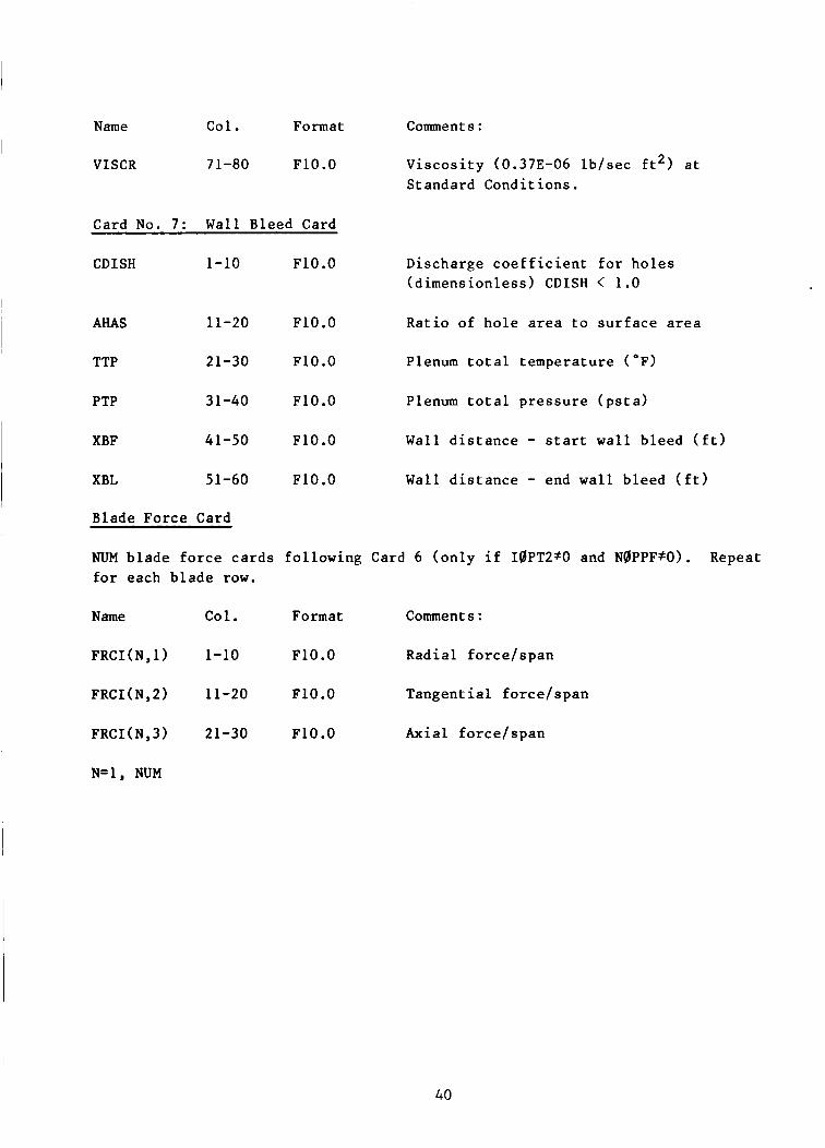
Name Col. Format
VISCR 71-80 F1O.O
Card No. 7 : Wall Bleed Card
CDISH 1-10
AHAS 11-20
TTP 21-30
PTP 3 1-40
XBF 41-50
XBL 51-60
Blade Force Card
NUM blade force cards for each blade row.
Name Col.
FRCI ( N, 1) 1-10
FRCI (N, 2) 11-20
FRCI(N,3) 21-30
N=l, NUM
F10 .O
F1O.O
F1O.O
F1O.O
F1O.O
F1O.O
Comments :
Viscosity (0.37E-06 lb/sec ft2) at Standard Conditions.
Discharge coefficient for holes (dimensionless) CDISH < 1.0
Ratio of hole area to surface area
Plenum total temperature (OF)
Plenum total pressure (psta)
Wall distance - start wall bleed (ft)
Wall distance - end wall bleed (ft)
following Card 6 (only if IQPT2fO and NQPPF#O). Repeat
Format Comments :
F1O.O Radial force/span
F1O.O Tangential force/span
F10 .O Axial forcelspan
40
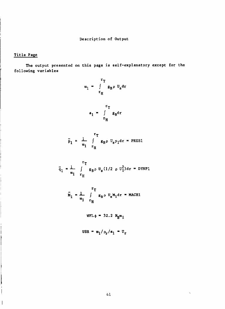
Description of Output
T i t l e Page
The output presented on t h i s page i s self-explanatory except for the following variables
'T 1 -
p1 = - I gBp Uspldr = PRES1 ml "
rm
WFL+ = 32.2 NBml
USR = ml/pr/al U,
41
I
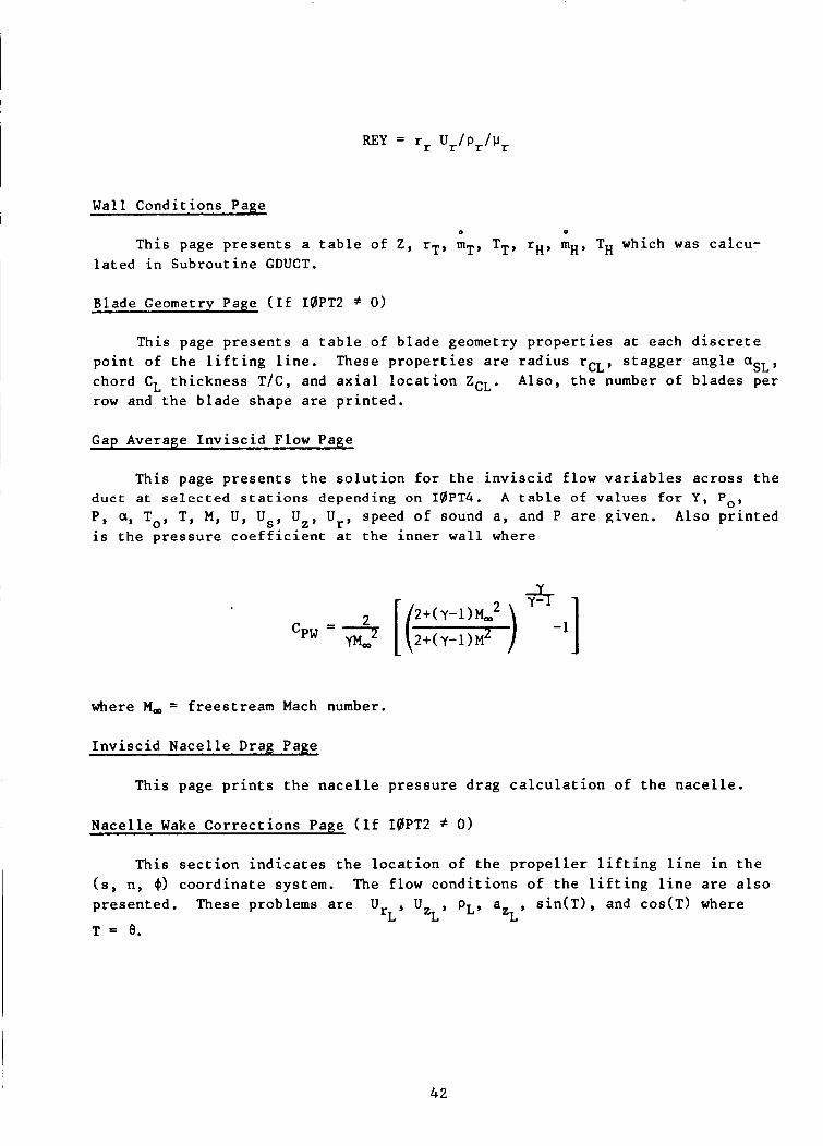
REY = rr Ur/pr/vr
Wall Conditions Page 0 0
This page presents a table of Z , rT, mT, TT, rH, mH, TH which was calcu- lated in Subroutine GDUCT.
Blade Geometry Page (If I0PT2 f 0)
This page presents a table of blade geometry properties at each discrete point of the lifting line. chord CL thickness T/C, and axial location ZcL. row and the blade shape are printed.
These properties are radius rcL, stagger angle aSL, Also, the number of blades per
Gap Average Inviscid Flow Page
This page presents the solution for the inviscid flow variables across the
Also printed duct at selected stations depending on IQPT4. P, a, To, T, M, U, Us, Uz, Ur, speed of sound a, and P are given. is the pressure coefficient at the inner wall where
A table of values for Y, Po,
2+(Y-1 >M,
cpw = 3 [ (2+(Y-1)MZ2) where M, = freestream Mach number.
Inviscid Nacelle Drag Page
This page prints the nacelle pressure drag calculation of the nacelle.
Nacelle Wake Corrections Page (If I0PT2 f 0)
This section indicates the location of the propeller lifting line in the ( s , n, 4) coordinate system. The flow conditions of the lifting line are also presented. These problems are U , U , PL, a , sin(T), and cos(T) where
T = 8. rL zL zL
42

Gap Average Viscous Flow Page
This page presents the solution for the flow variables across the duct at selected streamwise stations depending on IQPT4. A table of values for Y,
M, no, eo, C are given where P
cp * (n - n(o,o))/ql
0
f$ the wall values for Z, m, Cf4, Cfs, Q are printed, where C
and Cfs are defined by
The one-dimensional characteristics of the flow are also given: area ratio A/A1, Mach number (isentropic flow) MI, incompressible and compressible flow pressure coefficient CPINC and CPCQMP.
Wall Surface Conditions Page
This output page presents a summary of the wall conditions along the length of the duct.
TWT# ASTs QST’ This includes ZH, CpH,‘CFH, TW” ASH, QSH, ZT, CPT, CFT,
Wall Radiation Summary Page
This output page presents a summary of information which is useful in computing radiation effects. area dAH, UT, located at point ( Z H , rH), (ZT, rT) with the sin (wall angle) is given.
The wall temperature Tm, TW, on a differential
Viscous Nacelle Drag Page
This page prints the nacelle pressure drag, pressure drag coefficient, friction drag, and friction drag coefficient of the nacelle.
43

I
IDBGQ Pages
Intermediate printouts which were used to debug the program may be called by setting the debug options IDBG@=l. input card. The user should refer to the program listing in each subroutine to determine the printout variables.
IDBGg may be specified on the option
Debug Print Out Subroutine - Purpose
IDBGl TURB - Debug IDBG2 FCQRCT - Debug
IDBG3 FLQWIN - Debug IDBG4 Not Used
IDBG5 SaLVI - Debug
IDBG6 C00R - Debug
IDBG7 FgRCE - Debug IDBG8 MINVRT - Debug
IDBG9 SMggTH - Debug IDBGlO GDUCT - Debug IDBGll Not Used
IDBG12 SQLVI - Debug #2
IDBGl3 CKINPT - Debug IDBG14 Set Number of Streamlines
IDBG15 Automatic Step Size Debug, Number of Streamlines Calculated (default 25)
IDBG16 Suppress Freestream Instability
IDBG17 Not Used
IDBG18 GEQMCL - Debug
IDBG19 WAKCQR - Debug
IDBG20 PERFNA and PERFN2 - Debug 44

Desc r ip t ion of F a i l u r e Modes
I
The n a c e l l e p o r t i o n of t h e computer program can diagnose t h e cause of c e r t a i n f a i l u r e modes f o r t h i s p o r t i o n of t h e a n a l y s i s and a p r i n t e d message of t h e fol lowing form i s g iven .
**DIAGNOSTIC NO. XX FOR ANNULAR DIFFUSER DECK**
The number XX i d e n t i f i e s t h e type of f a i l u r e from t h e l i s t below.
1 ) IgPT3 OUTSIDE RANGE OF ALLOWABLE DUCT OPTIONS
This f a i l u r e occurs i n Subrout ine ALTMN. The input op t ion must be between 1 - < IBPT3 6 .
2 ) No s o l u t i o n e x i s t s i n AMFOR
This f a i l u r e occurs i n Subrout ine AMFOR. This subrou t ine so lves t h e Mach number func t ion
N = M (1 + ?)'I2/ ( 1 + +2)
f o r M given N. This func t ion has a maximum a t M = 1. Hence
So lu t ions do not e x i s t f o r va lues of N > N(1).
MASS FLOW EXCEEDS THE MAXIMUM MASS FLOW POSSIBLE 3)
This f a i l u r e occurs i n Subrout ine AMINLT which so lves t h e Mach number func t ion
for M given N. This func t ion has a maximum fo r M = 1 given by
corresponding t o choked flow.
45

Not Used
FOR BEST RESULTS ADD A STRAIGHT ANNULAR CHANNEL INLET
This d i a g n o s t i c occurs i n Subroutine C00R1. duc t c o o r d i n a t e s , i t is assumed t h a t t h e i n l e t has no c u r v a t u r e as shown i n f i g u r e 8. may be t o l e r a t e d . In o r d e r t o avoid problems, t h e b e s t procedure i s t o add a s t r a i g h t annular s e c t i o n t o t h e i n l e t a s shown by t h e d o t t e d l i n e i n f i g u r e 8.
- In t h e c o n s t r u c t i o n of t h e
This i s no t a f a t a l e r r o r because small i n l e t c u r v a t u r e s
PROGRAM ASSUMES INLET FLOW HAS CURVATURE
This d i a g n o s t i c occurs i n Subroutine C 0 0 R l . Same as d i a g n o s t i c 5 .
WALL CURVATURE IS TOO LARGE AT STATION X.
This d i a g n o s t i c occurs i n Subrout ine C 0 0 R l u s u a l l y with bad inpu t d a t a describing the duct contour resulting in a numerically discontinuous change i n w a l l c u r v a t u r e shown i n f i g u r e 2.
Not Ueed
GREATER THAN 1. PERCENT NORMAL PRESSURE GRADIENT ERROR RECALCULATE STATIC PRESSURE
This d i a g n o s t i c occur s i n Subrout ine ERPIN. This s u b r o u t i n e i n t e g r a t e s t h e r a d i a l e q u i l i b r i u m equa t ion
1
and compares (PT- P,) t o t h a t computed f o r t h e inpu t i n l e t f low (PT-PH)l. I f t h e error g i v e n by
i s g r e a t e r t h a n 0.01, t h e inpu t i n i t i a l s t a t i c p r e s s u r e d i s t r i b u t i o n is r ep laced by t h e above p r e s s u r e equa t ion and t h e flow is r e c a l c u l a t e d .
10) Not Used
46

11)
12)
13)
14)
15 1
16)
MASS FLOW REQUIRED EXCEEDS MAXIMUM MASS FLOW POSSIBLE
This d i a g n o s t i c occurs i n Subroutine CKINPT. Choked flow may e x i s t i n t h e d u c t , and t h i s d i a g n o s t i c w i l l be p r i n t e d o u t . be reduced.
The weight flow m u s t
PRESSURE RISE EXCEEDS PERMISSIBLE PRESSURE RISE
This d i a g n o s t i c occurs i n Subroutine CKINPT. f a i l u r e by t h e deck t o p rope r ly se t up flow e n t e r i n g d u c t . f o r e r r o r s .
This e r r o r occurs with the Check inpu t
Not Used
BOUNDARY LAYER TOO T H I N FOR MESH SPACING
This d i a g n o s t i c occurs i n Subroutine FLBWIN. The v i s c o u s flow c a l c u l a - t i o n r e q u i r e s a f i n i t e i n i t i a l boundary l a y e r t h i c k n e s s . r e q u i r e s enough mesh p o i n t s t o d e s c r i b e t h e i n l e t boundary v e l o c i t y p r o f i l e . r e q u i r e d . Thus, i f t h i s d i a g n o s t i c occur s , i n c r e a s e t h e number of mesh p o i n t s , KL, i n c r e a s e t h e mesh d i s t o r t i o n parameter, DDS, o r i n c r e a s e t h e assumed i n l e t boundary l a y e r t h i ckness . sets t h e mesh d i s t o r t i o n parameter f o r t u r b u l e n t flow.
In a d d i t i o n , i t
The deck assumes a r b i t r a r i l y t h a t a t least f i v e mesh p o i n t s are
S e t t i n g DDS = 0 a u t o m a t i c a l l y
TOTAL PRESSURE IS LESS THAN STATIC PRESSURE
This d i a g n o s t i c occurs i n Subroutine FLBWIN. inpu t d a t a f o r IgPTl
A check i s made on t h e 4, t o be s u r e t h a t PT > P.
INPUT DATA NOT I N RADIAL EQUILIBRIUM CORRECTIONS APPLIED TO STATIC PRESSURE
This d i a g n o s t i c occurs i n Subroutine FLgWIN. input d a t a f o r IgPTl = 4. i e assumed t h a t t h e s t a t i c p r e s s u r e i s i n e r r o r , and t h e o t h e r i n l e t d a t a i s c o r r e c t . Then t h e s ta t ic p r e s s u r e i s computed from
A check i s made o f t he I f t h e d a t a i s n o t i n r a d i a l equ i l ib r ium, i t
wi th t h e I D w a l l s t a t i c p r e s s u r e as a boundary c o n d i t i o n .
47

1 7 ) INPUT DDS MUST BE SPECIFIED
This diagnostic occurs in Subroutine FN0RM. At this time there is no algorithm to automatically select the mesh distortion parameter DDS for laminar flow.
18) BLADE DATA ERROR IN CKINPT ROUTINE
This diagnostic occurs in Subroutine CKINPT. Blade data input is incorrect. It must be rearranged with increasing Y.
1 9 ) NO UNIQUE SOLUTION FROM MINVRT
This diagnostic occurs in Subroutine MINVRT. If the matrix set up to solve the turbulent flow solution is singular, no solution can be obtained. This may occur from numerical truncation error problems.
20) LEADING OR TRAILING EDGE INDEX OF STRUT OUT OF RANGE
This diagnostic occurs in Subroutine SLETE. In order to compute blade forces, the strut must be wholly contained within the duct length. This problem may be eliminated by extending the duct length in a realistic manner as shown in figure 10.
21) Not Used
2 2 ) Not Used
23) BOUNDARY LAYER OVERLAP OR TOO LARGE
This diagnostic occurs in Subroutine FLgWIN. For internal flow, the sum of the two boundary layer thicknesses must be less than the duct inlet height. Check input data.
24) SET TOTAL TEMPERATURE, PRESSURE; ANGLE TO VALUE AT EDGE OF BOUNDARY LAYER - CORRECTIONS APPLIED This diagnostic occurs in Subroutine FLOWIN. For 10PTl = 4 , calculated boundary layer profiles are matched to experimentally measured inlet flow. Good matching occurs only if the inlet flow data shows constant PT in the boundary layer region as shown in figure 11 by the dotted line.
48

2 5 )
26)
27)
28
2 9 )
30 1
31 1
32
TRUNCATION ERROR CANNOT BE REDUCED BY STEP SIZE
This diagnostic occurs in Subroutine SQLVI. When the step size KDS is not specified, it is automatically selected by checking the truncation error at each step. When an instability occurs, the program attempts to reduce the truncation error by reducing the streamwise step. .If the truncation error cannot be reduced below a minimum value, the calculation stops with this error message.
NUMERICAL INSTABILITY
This failure occurs in Subroutine FCgRCT. Temperature and pressure are checked for negative values. Calculation stops with this error.
Not Used
Not Used
SOLUTION REQUIRES REVERSE FLOW, INCREASE WFLOW
This diagnostic occurs in Subroutine CKINPT. For flows with radial pressure gradients, there is a minimum weight flow below which reverse flow exists. This is corrected by increasing weight flow.
Not Used
Not Used
NORMAL COORDINATE OF LIFTING LINE IS NEGATIVE BLADE DATA DOES NOT CORRESPOND TO GEOMETRY OF DUCT
This diagnostic occurs in Subroutine GEgMCL. Blade geometry was inputted incorrectly to program. This will produce a fatal error.
49

DETAILED PROGRAM DOCUMENTATION
This s e c t i o n is intended t o provide s u f f i c i e n t documentation t o the use r so t h a t t he i n t e r n a l ope ra t ion of the program can be r e l a t e d t o the a n a l y s i s presented i n the t echn ica l r epor t (Reference 1 ) . It is assumed t h a t t he user d e s i r i n g t h i s informat ion has the requi red background i n aerodynamics and computat ional f l u i d dynamics or access t o the requi red t e c h n i c a l support t o understand the p e r t i n e n t a spec t s of the program code as they re la te t o the theory .
This s e c t i o n con ta ins two major subsec t ions , the p r o p e l l e r s o l u t i o n p o r t i o n and the n a c e l l e s o l u t i o n po r t ion , r e s p e c t i v e l y . These subsec t ions con ta in , (1 ) an a lphabe t i c l i s t of t he sub rou t ines and e x t e r n a l func t ions and a b r i e f d e s c t i p t i o n of each, (2 ) a more d e t a i l e d d e s c r i p t i o n of each sub- r o u t i n e i n a l p h a b e t i c a l o rde r and, ( 3 ) a d e s c r i p t i o n of t he l a b e l common b locks and v a r i a b l e s used i n a l p h a b e t i c a l o rde r . Flow c h a r t s and f i g u r e s are provided i n the sub rou t ine d e s c r i p t i o n s where deemed necessary to unders tand t h e program s t r u c t u r e and t e c h n i c a l f e a t u r e s .
The subrou t ines and e x t e r n a l func t ions are a l l descr ibed with the same format us ing the name of t he sub rou t ine wi th i t s argument l ist given as a t i t l e . A l i s t of op t ions and FORTRAN symbols used only i n the named sub- r o u t i n e are then given. Any s p e c i a l or a d d i t i o n a l theory used i n the subrou- t i n e is presented but w e l l known numerical methods are not descr ibed .
50

P r o p e l l e r Program
Within t h i s s e c t i o n b r i e f d e s c r i p t i o n s of t he sub rou t ines used i n t h e l i f t i n g l i n e p o r t i o n of t he a n a l y s i s are presented followed by the labe led common blocks used i n the a n a l y s i s . The o b j e c t i v e of a p a r t i c u l a r sub rou t ine is noted, along with a l i s t of symbols which are not i n l abe led common blocks and which are f e l t to be necessary f o r t he understanding of t he p a r t i c u l a r sub rou t ines i n ques t ion . These l i s t s of symbols have been kept b r i e f . A b r i e f exp lana t ion of t he theory is a l s o included f o r s e l e c t e d subrou t ines . Genera l ly , d e s c r i p t i o n s of t he opt ions which c o n t r o l t h e flow of a p a r t i c u l a r sub rou t ine are a l s o included. The subrou t ines are presented i n a l p h a b e t i c a l o rde r . The l abe led common blocks used i n t h e a n a l y s i s are a l s o l i s t e d i n a l p h a b e t i c a l o rde r wi th b r i e f d e s c r i p t i o n s of each v a r i a b l e re ferenced . Br i e f f low diagrams of t he major computat ional subrout ines (GCWAKE, PRflP, SQLVEL and SgLVEN) are included i n the d e s c r i p t i o n of each of t hese sub rou t ines .
L i s t of Subrou t ines ---------- Name D e s c r i p t i o n - AFFIDC C a l c u l a t e b lade a c t i v i t y f a c t o r and i n t e g r a t e d
des ign l i f t c o e f f i c i e n t
AF65A C a l c u l a t e cascade a i r f o i l d a t a
A I R = Cont ro l type of a i r f o i l d a t a t o be used
AIRFLT A i r f o i l package c o n t r o l r o u t i n e
AIRFMN
AIR23
Main a i r f o i l package c o n t r o l r o u t i n e f o r i n t e r - f ac ing i n t e r p o l a t i o n , cascade d a t a and i s o l a t e d a i r f o i l d a t a
Cont ro l l i f t and drag c a l c u l a t i o n s f o r a i r f o i l type number 23
AIR24 Cont ro l l i f t and drag c a l c u l a t i o n s for a i r f o i l
ASSOC
AVECTR
BILINE
BLDGE0
type number 24
Tes t input v a r i a b l e l a b e l
Create a column v e c t o r from sca
I n t e r p o l a t i o n r o u t i n e
C a l c u 1 ate b 1 ade geometry
ar input va lues
51

Name
CALCGC
CALWAK
CASARF
-
CASDAT
CHKINP
CLFACT
c0MBwK
CP ITER
CR0 S SP
CSCDl
CTITER
I D0TP
DRAG24
I DZR0A.L
ELIP2
FINAIR
FSQRT
FVECTR
GAUSS
GCBgLJN
Descr iDtion
Ca lcu la t e geometric i n f luence c o e f f i c i e n t
Control flow of wake geometry c a l c u l a t i o n s
Control r o u t i n e f o r a n a l y t i c a l cascade c o r r e c t i o n
Control s e l e c t i o n of type of cascade d a t a
Check input parameters f o r obvious e r r o r s
Ca lcu la t e l i f t curve s lope f a c t o r
Ca lcu la t e e f f e c t i v e displacement of bound v o r t e x
Ca lcu la t e b lade angle f o r next power performance i t e r a t i o n
Ca lcu la t e c r o s s product of two v e c t o r s
Cascade a i r f o i l d a t a sub rou t ine ( r e f e r e n c e - C a l c u l a t e b lade angle f o r next t h r u s t performance i t e r a t i o n
C a l c u l a t e do t product of two v e c t o r s
C a l c u l a t e drag c o e f f i c i e n t f o r a i r f o i l t ype number 24
C a l c u l a t e l i f t o f f s e t due to cascade i n f l u e n c e
Approximate E l l i p t i c I n t e g r a l of second kind
Cont ro l f i n a l a i r f o i l d a t a c a l c u l a t i o n
Ca lcu la t e magnitude of t h r e e component v e c t o r
Ca lcu la t e b lade f o r c e s
Solve system of s imultaneous l i n e a r equa t ions ( d i r ec t m e t hod
Ca lcu la t e geometr ic i n f luence c o e f f i c i e n t s f o r bound vor t ex
5 2

I - Name
, GCCQ RE 1
GCFILA ~
GCWAKE
I G4OOLD
INDVEL I INTIAL
~ 1 ISQAFL
ISQARF I LDDATA
I LIFT24
I
LINEAR
LINTER
1 MVMULT I I t MC@ NE
NSTAC$ 1 PAGE
PCH$UT
PERFQR
PERIQD
Description
Calculate vortex core model
Calculate geometric influence coefficient for trailing vortex filament
Control basic flaw of geometric influence coefficient calculations
Calculate lift and drag using linearized airfoil data
Calculate induced velocities
Initialize data and print out selected quantities
Control selection of isolated airfoil data type
Control isolated airfoil data calculation
Read in propeller data
Calculate lift coefficient for airfoil type number 24
Linear interpolation algorithm
Control interpolation of data arrays
Multiply single dimension vector with two dimensional vector
Calculate Evvard Tip Relief Correction
Calculate Mach cone intersection station index
Advance output device to new page
Punch spanwise distributions of aerodynamic quantities
Calculate propeller performance
Calculate propeller periodicity quantities
53

Desc r ip t ion Name
PERPRT
-
PHICAL
PLABEL
PN
PRQP
PRDATA
PRG400
PRINTP
PRTF 15
PRTF 1 6
PRTGCM
PRTI 15
PRTI16
PRTLF
PRTLI
PRTRZW
PRWZW
RDSCAL
RDVECT
P r i n t spanwise d i s t r i b u t i o n s of aerodynamic and geometric q u a n t i t i e s
Ca lcu la t e wake azimuth informat ion
P r i n t a l a b e l
C a l c u l a t e a s p e c i a l func t ion
Main p r o p e l l e r sub rou t ine
P r i n t l a b e l and v e c t o r
Write ou tput q u a n t i t i e s f o r a e r o e l a s t i c response a n a l y s i s ( r e f e r e n c e 12)
P r i n t l a b e l and v e c t o r
P r i n t l a b e l and f l o a t i n g poin t v a r i a b l e v e c t o r , maximum of 15
P r i n t l a b e l and f l o a t i n g po in t v a r i a b l e v e c t o r , maximum of 16
P r i n t geometric i n f luence c o e f f i c i e n t ma t r ix
P r i n t l a b e l and i n t e g e r index f o r maximum of 15 i n t e g e r s
P r i n t l a b e l and i n t e g e r index f o r maximum of 16 i n t e g e r s
P r i n t l a b e l f i e l d and s i n g l e f l o a t i n g p o i n t v a r i a b l e
P r i n t s i n g l e i n t e g e r and l a b e l
P r i n t r a d i a l o r a x i a l wake c o o r d i n a t e s
P r i n t wake geometry
Con t ro l s read of s c a l a r i n p u t s
Con t ro l s read of v e c t o r i n p u t s
54
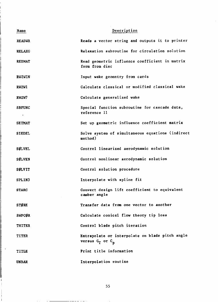
1 Name - READWR
RELAXG
REDMAT
RWZWIN
RWZWl
RWZW7
SBFUNC
SE TMAT
SIEDEL
SBLVEL
SgLVEN
SQLVIT
SPLIN3
STARC
STQRE
SWPCBR
THITER
TITER
TITLE
UNBAR
Description
Reads a vector string and outputs it to printer
Relaxation subroutine for circulation solution
Read geometric influence coefficient in matrix form from disc
Input wake geometry from cards
Calculate classical or modified classical wake
Calculate generalized wake
Special function subroutine for cascade data, reference 11
Set up geometric influence coefficient matrix
Solve system of simultaneous equations (indirect met hod
Control linearized aerodynamic solution
Control nonlinear aerodynamic solution
Control solution procedure
Interpolate with spline fit
Convert design lift coefficient to equivalent camber angle
Transfer data from one vector to another
Calculate conical flow theory tip loss
Control blade pitch iteration
Extrapolate or interpolate on blade pitch angle versus f+ or C P
Print title information
Interpolation routine
55

Name
UNINT
-
VECTQR
WECTR
Desc r ip t ion
I n t e r p o l a t i o n r o u t i n e
Compute v e l o c i t y and v e l o c i t y r e l a t e d q u a n t i t i e s inc luding induced v e l o c i t i e s
Compute v e l o c i t y and v e l o c i t y r e l a t e d q u a n t i t i e s inc luding induced v e l o c i t i e s
WAKMQD Modify wake geometry due t o n a c e l l e i n f l u e n c e
WRITGC Write geometric i n f luence c o e f f i c i e n t t o d i s c
ZERQAL C a l c u l a t e zero l i f t ang le
ZERQGC Se t i n f luence c o e f f i c i e n t matrices t o z e r o
DeSCriDtiOn o f t h e Subrout ines Used i n t h e ProDel le r Portj-on
Subrout ine AFFIDC (ITQT, DECL, BQD, SC0, AF, C L I , X , XB, R)
Object To c a l c u l a t e t he b lade a c t i v i t y f a c t o r and i n t e g r a t e d des ign l i f t c o e f f i c i e n t .
L i s t o f Swnbols
AF Blade a c t i v i t y f a c t o r C L I I n t e g r a t e d des ign l i f t c o e f f i c i e n t
Theory
The a c t i v i t y f a c t o r is def ined as
1
AF = j s co (;) ($ d(f)
56

where C/D is the blade chord t o p r o p e l l e r diameter r a t i o and x is the spanwise l o c a t i o n along the b lades .
The i n t e g r a t e d design l i f t c o e f f i c i e n t is
where SCQ is the root cu tout and CQd is the s e c t i o n design l i f t c o e f f i c i e n t .
Subrout ine AF65A (Argument L i s t )
Object Compute a i r f o i l l i f t and drag from cascade c o r r e l a t i o n s .
L i s t of Symbols
Arugment L i s t
AMACH ALP TM THETA CB
CL s °K) CD'l)
Cascade C o r r e l a t i o n
ALPS ALP 1 P H I C AKDELS AMSIG B DEL AKDELT DEL0 AI 00 AN AKIT
O1
4, k6S
&OO
K & t 6O
io0 n
K i t
b
9
S
D
S
S
a
D
S
S
S
, S
S
S
a
a
a
8
S
1
Upstream Mach number Angle of Attack Maximum A i r f o i l Thickness P i t c h angle Design L i f t C o e f f i c i e n t Cascade S o l i d i t y L i f t Coe f f i c i en t Drag Coef f i c i en t
( INPUT 1 ( INPUT 1 (INPUT) ( INPUT)
( INPUT 1 ( INPUT)
(OUTPUT) (OUTPUT)
Stagger Angle (deg rees ) I n l e t A i r Angle (deg rees ) Camber Angle Shape Parameters Camber Parameter Exponent Devia t ion Angle, +c= 0 Thickness Parameter Devia t ion Angle (degrees) Incidence Angle, oc= 0 (degeees) Power Thickness Parameter
57

AIM0 D ZLQ SM
ZL0SS AINCO
DALST ALPH2 RH0 cx
, Minimum Loss Incidence Angle (degrees) imo D , Diffusion Parameter
, Minimum Loss Coefficient sm i , Incidence Angle (degrees)
, Loss Coefficient , Stall Angle Correction , Exit Air Angle
z S
a2 (PU~)~/(PU~)~ , Mass Flow Ratio
Additional Symbols
( a 2 , 2,) + (CL, $1
T1 AMACH2 T2 P02P01 P2P1 FS FP ws w ALIND ANG
Upstream Total Static Temperatures Downstream Mach Number Downstream Total Stat:ic Temperature Total Pressure Ratio Static Pressure Ratio Streamwise Force Coefficient Tangential Force Coefficient Streamwise Induced Velocity Tangential Induced Velocity Induced Flow Angle Angle of Attack
Theory See section of reference 1 entitled: “Cascade Airfoil Data”.
Subroutine AIRFL
Object Controls which type of airfoil data will be used, either isolated data or isolated data corrected for cascade effects.
Options IDL = 0 print title IDL f 0 obtain airfoil data ICASDE = 0 obtain isolated airfoil data ICASDE = 1 obtain isolated airfoil data corrected for cascade
effects
58
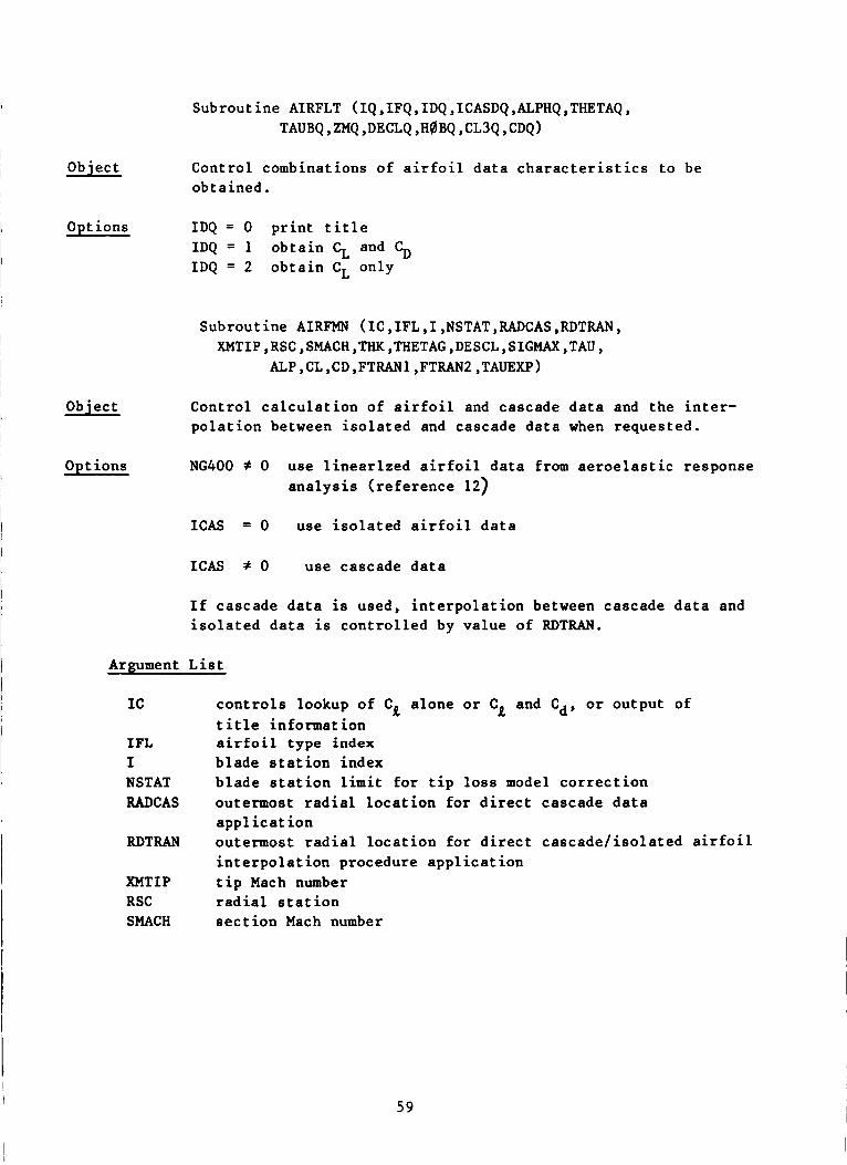
Objec t ~
I Opt ions
Object 1
Options I
Subrout ine AIRFLT (IQ,IFQ,IDQ,ICASDQ,ALPHQ,THETAQ, TAUBQ,ZMQ,DECLQ,H(dBQ ,CL3Q,CDQ)
Cont ro l combinations of a i r f o i l d a t a c h a r a c t e r i s t i c s t o be obta ined . I D Q = 0 p r i n t t i t l e I D Q = 1 I D Q = 2
o b t a i n (+, and % o b t a i n CL only
Subrout ine AIRFMN (IC,IFL,I,NSTAT,RADCAS,RDTRAN, XMTIP , RSC , SMACH ,THK ,THETAG, DESCL , SIGMAX ,TAU,
ALP, CL , CD , FTRAN 1 , FTRAN2 , TAUEXP )
Contro l c a l c u l a t i o n of a i r f o i l and cascade d a t a and t h e i n t e r - p o l a t i o n between i s o l a t e d and cascade d a t a when reques ted .
NG400 f 0 use l i n e a r l z e d a i r f o i l d a t a from a e r o e l a s t i c response a n a l y s i s ( r e f e r e n c e 12)
ICAS = 0 use i s o l a t e d a i r f o i l d a t a
ICAS f 0 use cascade d a t a
I f cascade d a t a i s used, i n t e r p o l a t i o n between cascade d a t a and i s o l a t e d d a t a is c o n t r o l l e d by va lue of RDTRAN.
Argument L i s t
I C
IFL I NSTAT RADCAS
RDTRAN
XMTIP RSC SMACH
c o n t r o l s lookup of CQ a lone o r CQ and cd, o r ou tput of t i t l e informat ion airfoil type index b lade s t a t i o n index b l a d e s t a t i o n l i m i t f o r t i p l o s s model c o r r e c t i o n outermost r a d i a l l o c a t i o n f o r d i r e c t cascade d a t a a p p l i c a t i o n outermost r a d i a l l o c a t i o n f o r d i r e c t c a s c a d e / i s o l a t e d a i r f o i l i n t e r p o l a t i o n procedure a p p l i c a t i o n t i p Mach number r a d i a l s t a t i o n s e c t i o n Mach number
5 9

THK THETAG DESCL S IGMAX TAU ALP CL CD FTRANl
RTRANl
TAUEXP
s e c t i o n s e c t i o n sect ion s e c t i on sect ion s e c t i o n s e c t ion s e c t i o n s e c t i o n
f o r CI1
f o r cd s e c t i o n c a s c a d e / a i r f o i l i n t e r p o l a t i o n s c a l i n g func t ion v a l u e
exponent used i n i n t e r p o l a t i o n f u n c t i o n
th i ckness r a t i o geometr ic p i t c h angle wi th t h e plane of r o t a t i o n des ign l i f t c o e f f i c i e n t s o l i d i t y gap t o chord r a t i o angle of a t t a c k 1 i f t c o e f f i c i e n t drag c o e f f i c i e n t c a s c a d e / a i r f o i l i n t e r p o l a t i o n s c a l i n g func t ion va lue
Subrout ine AIR23
Object Ca lcu la t e Manoni a i r f o i l c h a r a c t e r i s t i c s from i n t e r n a l l y t a b u l a t e d d a t a bank us ing t r anson ic s i m u l a r i t y r u l e s .
Opt i ons I D L = 1 o b t a i n CL
IDL = 2 o b t a i n CD
IDL = 3 dummy f e a t u r e
Theory
Using t r a n s o n i c s i m u l a r i t y r u l e s , empi r i ca l d a t a has been reduced t o a set of t a b u l a t e d c o e f f i c i e n t s which can be used t o r e c o n s t r u c t t h e a i r f o i l c h a r a c t e r i s t i c s (C, and CD> for a wide range o f parameters .
Subrout ine AIR24
Object Control s e l e c t i o n of c a l c u l a t i o n of l i f t or drag c o e f f i c i e n t s f o r the publ i shed NACA d a t a .
Options IDL = 1 o b t a i n l i f t
IDL = 2 o b t a i n d rag
IDL 3 dummy f e a t u r e
60

Subroutine AsS0C (*,S,FDUM,Sl,S2,X)
Object To transfer input value of a dummy parameter to its correct allocation if the input label matches one in the argument list. If transfer is made, returns to labeled statement in calling routine .
Argument List
S input label as read FDUM input dummy parameter Sl,S2 input label list X allocation for transfer of dummy parameter
Subroutine AVECTR (A1 ,A2 ,A3 ,VI
Object load three scalars into a vector of length three.
Argument L is t
A1 ,A2 ,A3 input scalars V output vector
Subroutine BILLNE (T,I,XI ,YI , Z , K )
Object Bivariant or univariant interpolation on input vectors using various interpolation options.
Opt ions T(I + 1) = 0 use first table value
T(I + 1) 1 use linear interpolation
T(I + 1) = 2 use third order interpolation
T(I + 3 ) = non zero, requests bivariant interpolation
Argument List
T = vector with interpolation data I = starting location for data table X I = input x for interpolation YI = input y for interpolation Z = output value K = error code
61

Theory
Opt ions NCBWAK = 0
NCBWAK 1
NCBWAK = 2
Using either bivariant or univariant data, this subroutine will interpolate on the data using standard interpolation schemes as noted above - see listing for more detail.
Subroutine BLDGEQ (IC)
Object Rotate input lifting line segment geometry to the requested blade angle about the pitch axis and compute the inflow station geometry for this blade angle. Print the table of the lifting line segment and center coordinates.
List of Symbols
IC = print control flag DR##P = angle between the coordinate origin (hub center) and
the axial displacement for the coordinate point in question for blade element center.
DR#@PB = angle between the coordinate origin (hub boundary) and the axial displacement for the coordinate point in question for the blade element boundary.
Theory Standard geometric operations applied to the input geometry to rotate the coordinates to a different blade angle position.
Subroutine CALCGC (Argument List)
Object To calculate the geometric influence coefficients for a selected field point in the cylindrical coordinate system,
no compressibility effects on the bound vortex induced velocity calculation
compressibility effects included on the bound vortex induced velocity calculations
compressibility effects included in the bound vortex induced velocity calculation, except for the calculation for the particular blade bound vortex system on itself
62

IJUNK = 0 no vortex core model
IJUNK = 1 vortex core model used
IDEBUG = 0 no intermediate printout
IDEBUG = 1 intermediate printout
NCQMPRS = 0 no wake compressibility model
NCQMPRS = 1 wake compressibility model used
NCFLQW = 0 wake compressibility applied only on vortex seg- ments from inflow sections with Mach numbers greater than 1 .O
NCFLBW = 1 relaxes the above restriction
Argument List
NCQMP compressible wake option switch I B I P = blade index LLINK = blade position index NBX = number of blades I T Q T number of blade element segments L T 0 T = number of blade positions KTQT = number of blade element boundaries MT0T number of filament segments KTRUCT = number of filaments for tip vortex rollup model JTRUCT = wake rollup truncation angle JTRUCI inboard wake truncation angle D P S I B R = azimuth interval in radians FS = sign (21.0) for axial induced velocity calculation R S C I =:‘radial location of field point P H I C I = lag angle of field point Z S C I = axial location of field point CPD = cosine of blade element angle SPD = sine of blade element angle RSBB ZSBB P H I B B CBSLB S I N L B CMACH = local blade element Mach number Mu = local blade element advance ratio DTIPM VQRCQR = vortex core radius
= blade element boundary radial position = blade element boundary axial position = blade element boundary azimuth position = blade element boundary cosine of azimuth position = blade element boundary sine of azimuth position
= blade tip Mach number
6 3
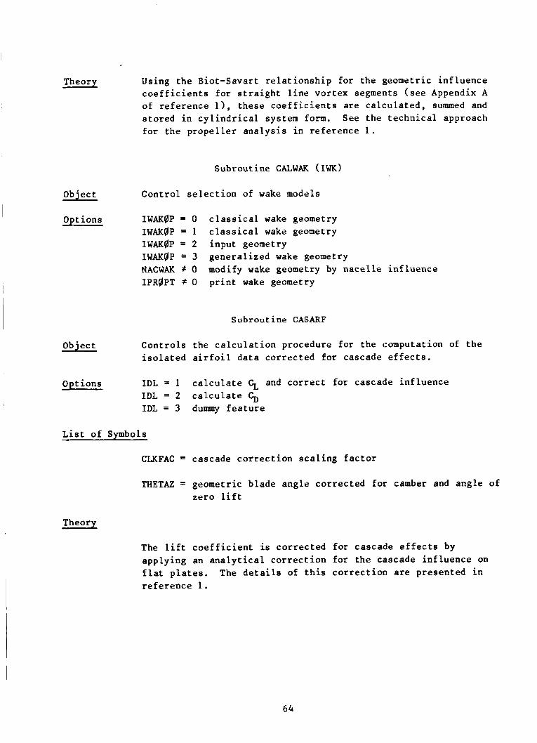
Theory Using the Biot-Savart relationship for the geometric influence coefficients for straight line vortex segments (see Appendix A of reference 11, these coefficients are calculated, summed and stored in cylindrical system form. See the technical approach for the propeller analysis in reference 1.
Subroutine CALWAK (IWK)
Object Control selection of wake models
Opt ions IWAKQP = 0 classical wake geometry IWAKQP = 1 classical wake geometry 1WAKQP = 2 input geometry IWAKQP = 3 generalized wake geometry NACWAK # 0 modify wake geometry by nacelle influence IPRQPT f 0 print wake geometry
Subroutine CASARF
Object Controls the calculation procedure for the computation of the isolated airfoil data corrected for cascade effects.
Options IDL = 1 calculate and correct for cascade influence IDL = 2 calculate % IDL = 3 dummy feature
List of Svmbols
CLKFAC = cascade correction scaling factor
THETA2 = geometric blade angle corrected for camber and angle of zero lift
Theory
The lift coefficient is corrected for cascade effects by applying an analytical correction for the cascade influence on flat plates. reference 1.
The details of this correction are presented in
64

Subrout ine CASDAT (Argument L i s t )
Obiect Cont ro l s e l e c t i o n of cascade d a t a source .
Opt ions ICAS = 0 t e rmina te execut ion of code ICAS = 1 I C A S = 2
cascade d a t a us ing c o r r e l a t i o n from r e f e r e n c e 13 cascade d a t a us ing model of r e f e r e n c e 11
Argument L i s t
ICAS = o p t i o n switch f o r type of cascade d a t a MACH = l o c a l s e c t i o n Mach number AL = l o c a l s e c t i o n angle of a t t a c k THK = l o c a l s e c t i o n th i ckness r a t i o THET = l o c a l s e c t i o n b lade ang le DESCLP = l o c a l s e c t i o n des ign l i f t c o e f f i c i e n t SIG = l o c a l s e c t i o n s o l i d i t y r a t i o CL = l o c a l s e c t i o n l i f t c o e f f i c i e n t CD = l o c a l s e c t i o n d rag c o e f f i c i e n t
Subrout ine CHKINP
Object To check input d a t a f o r c o r r e c t input va lues on s e l e c t e d i t e m s and make s u r e items t h a t are necessary f o r s u c c e s s f u l execu t ion are inpu t .
Subrout ine CLFACT (THETA,TAUB,CLKFAC)
Objec t Obta in t ab led va lue of l i f t curve s l o p e s c a l i n g f a c t o r f o r i n p u t parameters .
L i s t of Symbols
THETA ze ro l i f t
TAUB = gap-to-chord r a t i o CLVFAC = l i f t curve s lope s c a l i n g f a c t o r
= geometric b lade angle co r rec t ed f o r camber and ang le o f
Theory Table of d a t a f o r t h e l i f t curve s lope s c a l i n g f a c t o r was der ived a n a l y t i c a l l y f o r f l a t p l a t e s by Weinig. d a t a w a s ob ta ined from r e f e r e n c e 4.
The t a b l e of
6 5
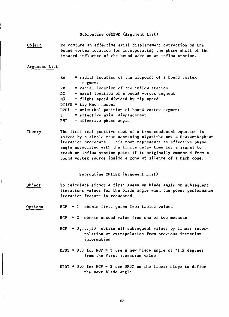
Subrout ine CgMBWK (Argument L i s t )
Object To compute an e f f e c t i v e a x i a l displacement c o r r e c t i o n on t h e bound vor t ex l o c a t i o n f o r i nco rpora t ing the phase s h i f t of the induced in f luence of t he bound wake on an inf low s t a t i o n .
Argument L i s t
RA = r a d i a l l o c a t i o n of t he midpoint of a bound v o r t e x
RB = r a d i a l l o c a t i o n of the inf low s t a t i o n DZ = a x i a l l o c a t i o n of a bound vor t ex segment MU = f l i g h t speed d iv ided by t i p speed DTIPM = t i p Mach number DPSL = azimuthal p o s i t i o n of bound vor t ex segment z = e f f e c t i v e a x i a l displacement PHI = e f f e c t i v e phase angle
segment
Theory The f i r s t real p o s i t i v e root of a t r anscenden ta l equat ion i s so lved by a s i m p l e root sea rch ing a lgo r i thm and a Newton-Raphson i t e r a t i o n procedure. Th i s roo t r e p r e s e n t s an e f f e c t i v e phase angle a s s o c i a t e d w i t h t he f i n i t e de lay t i m e f o r a s i g n a l t o reach an inf low s t a t i o n poin t i f i t o r i g i n a l l y emanated from a bound vor t ex source i n s i d e a zone of s i l e n c e of a Mach cone.
Subrout ine CPITER (Argument L i s t )
Objec t To c a l c u l a t e e i t h e r a f i r s t guess on b lade angle or subsequent i t e r a t i o n s va lues f o r t he b lade angle when t h e power performance i t e r a t i o n f e a t u r e i s reques ted .
Opt ions NCP = 1 o b t a i n f i r s t guess from t ab led va lues
NCP = 2 o b t a i n second value from one of two methods
N C P = 3 , . . . , l o o b t a i n a l l subsequent va lues by l i n e a r i n t e r - p o l a t i o n or e x t r a p o l a t i o n from previous i t e r a t i o n informat ion
DPDT = 0.0 f o r N C P = 2 use a new b lade angle of ?I .5 degrees from the f i r s t i t e r a t i o n v a l u e
DPDT f 0.0 f o r N C P = 2 use DPDT as t h e l i n e a r s l o p e to d e f i n e t h e next b lade angle
66

Argument List
I Theory I
Object
ITaT = number of blade elements BL = number of blades ZJI advance ratio RSC = inflow station segment radial centers RSB = inflow station boundary radial locations DESCL = design lift coefficient B0D = chord over diameter ratio CPWANT = requested power coefficient DPDT = input linear slope of the power coefficient versus
RAD = blade radius blade angle relationship
Using standard interpolation and extrapolation techniques, the blade angle for each iteration of the power performance itera- tion is determined. For the first iteration tabled values are used if requested and for the second iteration one of two methods can be used to determine the new blade angle. All subsequent iteration values are obtained using linear extrapola- tion or interpolation based on previous iteration information.
Subroutine CRQSSP (V,A,Rl ,R2 ,R3)
Calculate cross product of two vectors and place results in three scalars.
67

Subroutine CSCDl (IND,CB,TH,SOL,ST,RN,AM,ILF,S:LF,CL,CD)
Object Calculate cascade lift and drag coefficients from reference 13.
Argument List
IND = controls selection of airfoil type CB = section camber TH = section thickness ratio SQIL = section solidity ST = section pitch angle RN AM = section angle of attack CL = section lift coefficient CD = section drag coefficient
= Reynolds number (fixed at 500000)
Subroutine CTITER (CTWANT ,DCTDT)
Object To calculate either the first or all subsequent blade angles when the thrust iteration has been requested.
Opt ions NCP = 1 use a fixed value of 60.0 degeees for the first guess NCP = 2 use one of the two methods to determine the second
value
NCP = 3,..,10 use linear interpolation or extrapolation based on the previous iterations to determine the next value
DCTDT = 0.0 for NCP = 2 use a new blade angle of 51.5 degrees from the first iteration value
DCTDT # 0.0 for NCP = 2 use the value of DCTDT as the linear slope to define the next blade angle
Theory Using standard interpolation and extrapolation techniques, the blade angle for each iteration of the thrust: iteration cycle is determined. For the first iteration, a fixed value is used if requested and for the second iteration one of two methods can be used to determine the new blade angle. All subsequent itera- tions values are obtained using linear interpolation or extrap- olation based on previous iteration informat:ion.
Subroutine DBTP (V ,A)
Object Calculate dot product of two vectors, each of length three.
68

Subroutine DRAG24
Object Calculate drag coefficient from the NACA airfoil data.
Theory Using linear interpolation techniques applied to a set of tabulated airfoil drag coefficients which are functions of Mach number, angle of attack, thickness to chord ratio and design lift coefficient, the drag coefficient is found for a specified combination of the above parameters (reference 1).
Subroutine DZRQAL (THSTAR ,TAUB ,THETAT ,DELAQL)
Object Determine increment in angle of zero lift for cascade correction procedure.
Argument List
THSTAR = effective blade camber angle TAUB = gap-to-chord ratio THETAT = effective blade angle DELAQL = increment in angle of zero lift
Theory Using trivariate interpolation t-echniques, the increment in the angle of zero lift is determined from a set of tabulated data for double circular arc aifoils (reference 5 ) .
Subroutine ELIP2 (XI
Object Calculate approximation for elliptic integral of the second kind.
Argument List
X = argument of approximation function
Subroutine FINAIR
Object Control final calculation procedure for airfoil characteristics.
Opt ions IDEBUG = 0 no printout IDEBUG > 0 printout of final values €or the airfoil
Characteristics is requested ICAS = 0 no cascade airfoil data is used ICAS f 0 cascade airfoil data is used out to a requested
radial location
69

Object
Theory
Function FSQRT (X ,Y ,Z)
Calculate magnitude of vector of components X, Y, and Z
FSQRT = (X2 + Y2 + Z2)li2
Argument List
X,Y,Z = components of vector FSQRT resultant
Subroutine FVECTR
Object Calculate components of blade forces at each blade inflow stat ion.
Opt ions IDEBUG f 0 request printout of component Eorces
L i s t of Svmbols
ALFLC = lift force in the chordwise direction ALFLN = lift force in the normalwise direction ALFLS = lift force in the spanwise direction ALFDC = drag force in the chordwise direction ALFDN = drag force in the normalwise direction ALFDS = drag force in the spanwise direction
Theory Using a calculated blade section lift and drag coefficients and the appropriate aerodynamic quantities, the forces in the blade element coordinate system are calculated and these forces are transformed to the cylindrical coordinate system.
Subroutine GAUSS (Augument List)
Object Solve a system of simultaneous linear equations in matrix form using a direct solution technique.
Argument List
NRdWM = row dimension of the coefficient matrix N = number of rows and columns used in the matrix solution A = coefficient matrix B = constant vector and on output contains the solution
vector
70

DET = mantissa of the value of the determinant in base ten IDET LSING = singularity flag
= integer power to the base ten of the determinant
- Theory Using a standard Gauss-Jordan reduction method a system of
simultaneous linear equations is solved and the detetminant of the matrix is calculated.
Subroutine GCBQUN (RSC,CP,SP,ZSC,RSB,ZSB,PHLB, CQSLB , SINLB , CMACH ,MU ,TIPM ,VC@R)
Object Calculate geometric influence coefficients at a specified load point for the bound vortex segments which represent the propeller blade lifting line.
Argument List
RSC = radial position of load point at which induced influence
CP cosine of azimuthal position of load point SP p sine of azimuthal position of load point ZSC = axial position of load point RSB = radial location of bound vortex segment endpoints PHIB = azimuthal position of bound vortex segment endpoints CQSLB = cosine of azimuthal position of bound vortex segment
SINLB = sine of azimuthal position of bound vortex segment
CMACH = mach number of bound vortex segment endpoints MU advance ratio of propeller disk TIPM = tip mach number of propeller disk VCQR = vortex core radius
is to be calculated
endpoints
endpoints
Theory Uses the potential flow solution for the induced influence of a finite length straight vortex filament, formulated in a cylindrical coordinate system. See Appendix B, Volume I.
71

Subroutine GCCqRE (IB,IFILA,IDEBUG,IFLAG,KARB, ZAZB , RASQ , RBSQ , CP , DSCA , DSCA ,VC~R)
Object Tabulate induced influence of a vortex segment if the load point is within the core radius.
Argument List
IB = type of vortex segment indicator (bound or trailing) IFILA = vortex segment number IDEBUG = debug output trigger IFLAG = flag
RARB = intermediate geometric quantity needed for the calculation, see Appendix B, Volume I
ZAZB = intermediate geometric quantity needed for the calculation, see Appendix B, Volume I
RASQ = intermediate geometric quantity needed for the calculation, see Appendix B, Volume I
RBSQ = intermediate geometric quantity needed for the calculation, see Appendix B, Volume I
CP = intermediate geometric quantity needed for the calculation, see Appendix B, Volume I
DSCA = intermediate geometric quantity needed for the calculation, see Appendix B, Volume I
DSCA = intermediate geometric quantity needed for the calculation, see Appendix B, Volume I
VC(6R = vortex core radius
Theory If the load point at which the induced influence due to a vortex segment is within a specified core radius, the induced influence is modeled by a solid body rotation model. This removes the singular behavior due to a purely potential flow vortex.
72

I I I
I
I
j
I
I
I I
I
Subroutine GCFlLA (K,NC$hlPT,IBIWK,LBTQT,LLIUK, RSCI ,CP ,SP ,ZSCI,KTRUCT,JTRUCT,JTRUCI ,MToT,KTQT,
LTQT,C0SLB,SINLB,DTIPM,VflRCaR)
Object Calculate geometric influence coefficients at a specified load point for the trailing vortex segments of a specified filament which represent the wake geometry.
Opt ions NCQMPT = 0 no compressible wake NC0MPT f 0 KTRUCT f 0
VgRC0R f 0
use compressible wake wake rollup model used beyond this filament index value vortex core option requested
Argument List
K = vortex filament index NCQMPT = option control for compressible wake model IBIWK = blade index for wake LBTQT = blade and rotor position index LLIWK RSCI = radial position of load point cp = cosine of azimuthal position of load point SP ZSCI = axial coordinate of load point KTRUCT = filament index defining boundary. for tip vortex rollup
JTRUCT = filament azimuth position index for wake truncation
JTRUCI 5 filament azimuth position index for wake truncation for
MT0T = number of segment endpoints KT0T = number of filaments LTQT = number of rotor positions C0SLB = cosine of filament azimuth position at blade SINLB = sine of filament azimuth position at blade DTIPM = reciprocal of blade tip Mach number VqRCQR vortex core radius
= rotor position index of wake
= sine of azimuthal position of load point
model
associated with tip rollup model
inboard wake
Theory Uses the potential flaw solution for finite length straight vortex segment, formulated in a cylindrical coordinate system. See Appendix B, Volume I.
73

Subrout ine GCWAKE
Object Con t ro l s flow of the geometric i n f luence c o e f f i c i e n t ca l cu la - t i o n s . A flow diagram is presented i n f i g u r e 12.
Opt i ons IWAK0P = 0 s tandard wake model (modified c l a s s i c a l wake)
input wake geometry gene ra l i zed wake model
p r i n t wake geometry
IWAKQP = 1 c l a s s i c a l wake model IWAKBP = 2 IWAKQP = 3 NACWAK f 0 o b t a i n n a c e l l e c o r r e c t i o n s f o r wake geometry IPRBPT f 0
Subrout ine G 4 O O L D (I,ALPHA,CL,CD)
Object C a l c u l a t e l i f t and drag a i r f o i l c h a r a c t e r i s t i c s ob ta ined from an e x t e r n a l source.
Argument L i s t
I = b lade segment index ALPHA = s e c t i o n angle of a t t a c k CL = s e c t i o n l i f t c o e f f i c i e n t CD = s e c t i o n drag c o e f f i c i e n t
Theory The l i f t and drag c h a r a c t e r i s t i c s f o r each b lade element segment are obta ined from an e x t e r n a l source by curve f i t t i n g a q u a d r a t i c polymonial about t he angle of a t t a c k at each s t a t i o n . The l i f t and drag are r econs t ruc t ed i n t h i s sub rou t ine f o r use i n t h e s o l u t i o n procedure.
Subrout ine INDVEL
Object Compute induced v e l o c i t i e s .
Opt ion IDEBUG f 0 p r i n t t he c a l c u l a t e d induced v e l o c i t i e s
Theory Reading t h e s t o r e d geometr ic i n f luence c o e f f i c i e n t s i n a de f ined o rde r from a d i s c , t h e induced v e l o c i t i e s are c a l c u l a t e d by mul t ip ly ing and summing over t h e appropr i a t e i n d i c e s of t h e m a t r i x quant i t ies .
74
I I
Object 1
Subroutine INTIAL
Object
Opt i ons
Object
Options
Object I I
Objec t
Theorv
To c a l c u l a t e s e l e c t e d d a t a and p r i n t o u t i n i t i a l input d a t a .
Subroutine ISgAFL
Cont ro l s e l e c t i o n of type of i s o l a t e d a i r f o i l d a t a t a b l e s t o use (Manoni or NACA) . IDL = 1 l i f t only IDL = 2 drag IDL = 3 dummy f e a t u r e IFL = 23 use Manoni d a t a I n = 24 use NACA d a t a IFL < 23 or > 24 use Manoni d a t a
Subrout ine ISgARF
Cont ro l the flow of i s o l a t e d a i r f o i l d a t a module.
IDL = 0 IDL = 1 compute l i f t IDL = 2 compute d rag
r e t u r n t o c a l l i n g r o u t i n e
Subrout ine LDDATA
Read i n r equ i r ed i n i t i a l p r o p e l l e r input d a t a and c a l c u l a t e s e l e c t e d d a t a from input q u a n t i t i e s .
Subrout ine LIFT24
C a l c u l a t e l i f t c o e f f i c i e n t from t a b u l a t e d a i r f o i l d a t a t a b l e s con ta in ing the NACA d a t a .
Using l i n e a r i n t e r p o l a t ion techniques t h i s sub rou t ine computes t h e l i f t c o e f f i c i e n t from a t a b l e of NACA a i r f o i l d a t a which is a func t ion of Mach number, angle of a t t a c k , des ign l i f t c o e f f i c i e n t and th i ckness t o chord r a t i o ( r e f e r e n c e 1).
75

Subroutine LINEAR (Argument List)
Object Interpolate and extrapolate linearly on an finput set of data.
Argument List
NW = print output file number N = number of data points in the interpolation vectors X I N = independent data vector Y I N = dependent data vector XQUT = requested interpolation point YdUT = interpolated value LQFF = interpolation flag
Theory Simple linear interpolation algorithm; if off scale on the low or high end, the flag is set (1 or 2 respect:ively) and the boundary slope is used to extrapolate t o the requested inter- polation point.
Subroutine LINTER (Argument List)
Object Control the interpolation of selected data arrays from input interpolation tables.
Opt ions NERR = 1 use lower boundary value NERR = 2 use upper boundary value
Argument List
N = number of data points in the interpolation vector K = number of requested interpolation points X I N = independent interpolation vector Y I N = dependent interpolation vector X Y = vector of interpolated values
= vector of requested interpolation points
76

Subrout ine MCQNE (Augument L i s t )
Object Ca lcu la t e Eward T i p Re l i e f Correc t ion .
Opt ions NEVARD = 0 no c o r r e c t i o n NEVARD = 1 used tab led va lues NEVARD = 2 use equat ion
Argument L i s t
NEVARD = opt ion c o n t r o l f o r method of c a l c u l a t i o n IP = p r o p e l l e r index L = p r o p e l l e r p o s i t i o n index RSC = r a d i a l l oca t ion of inf low s t a t i o n C = chord R = p r o p e l l e r r ad ius ITQIT = number of inf low s t a t i o n s CNSECT = f r a c t i o n of chord XMTIP = t i p Mach number NSTAT = s t a t i o n index f o r boundary fo r Mach cone i n t e r s e c t i o n =CONE = t i p r e l i e f c o r r e c t i o n vec to r RTIP = t i p r ad ius
Theory See s e c t i o n of r e fe rence 1 e n t i t l e d : "Evvard T i p Re l i e f f o r P r ope 1 1 er s " .
Subrout ine MVMULT (V,M,Rl ,R2 ,R3)
Object Mul t ip ly a t h r e e by t h r e e mat r ix by a vec to r of length t h r e e . S t o r e the resu l t i n t h r e e s e p a r a t e s c a l a r s .
Argument L i s t
V = v e c t o r M = matrix R1 ,R2 , R 3 = r e s u l t a n t s c a l a r s
77

Subroutine NSTAC0 (Argument List)
NUNIT = output file number
Object Calculate Mach Cone intersection station index.
Options IDEBUG > 0 requests printout of selected data
Argument List
NSTAT = station index where intersection occurs XMTIP tip Mach number IP = propeller index L = propeller position index
Theory Using relative geometry the angle XNETA is computed for each station and compared with the Mach cone angle, BETA, until the station where the intersection of the Mach cone with the specified fraction of the blade chord is determined.
Subroutine PAGE (NWRITE)
Object Print new page.
Argument List
NWRITE = print output file number
Subroutine PCH0UT (NUNIT)
Object Output spanwise distributions of aerodynamic and geometric quantities to specified output device number,
Areumen t List
78
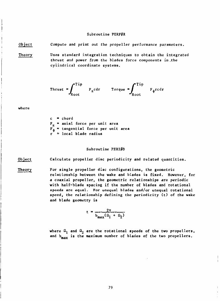
Subroutine PERFQR
Object
Theory
Compute and print out the propeller performance parameters.
Uses standard integration techniques to obtain the integrated thrust and power from the blades force components in .the cylindrical coordinate systems.
Thrust = F,cdr Torque a
I where
c = chord F, = axial force per unit area F 4 = tangential force per unit area r = local blade radius
Subroutine PERI$D
Object
Theory
Calculate propeller disc periodicity and related quantities.
For single propeller disc configurations, the geometric relationship between the wake and blades is fixed. However, for a coaxial propeller, the geometric relationships are periodic with half-blade spacing if the number of blades and rotational speeds are equal. speed, the relationship defining the periodicity (t> of the wake and blade geometry is
For unequal blades and/or unequal rotational
where Q, and S12 are the rotational speeds of the two propellers, and bmax is the maximum number of blades of the two propellers.
79

Subroutine PERPRT (NW,L,IP)
Object Print spanwise distributions of aerodynamic and geometric quantities to a specified output unit.
Argument List
NW = output unit number L = propeller position index IP = propeller index
Subroutine PHICAL (MT@T,DPSI)
Object Compute wake azimuth positions and trigonometric relationships for all propeller azimuth positions.
I Argument List
MTgT = number of wake filament segments DPSI = azimuthal increment
Theory Using the requested blade azimuth increment, the wake azimuth position and the sine and cosine functions for such are computed and stored. The fact that the sine and cosine functions are periodic is made use of to reduce the actual number of sine and cosine values which are stored.
Subroutine PLABEL (NWRITE,NSLB,NSLF,NSP,NL,LABEL)
Object Print a label field.
Argument List
NWRITE = output device number NSLB = number of lines to skip before label is output NSLF = number of lines to skip after label is output NSP = number of units of 10 spaces to skip before label is
NL = length of label in increments of 6 LABEL = label vector
output
80

Function PN (N,R,S)
Object Compute special functions of R and S.
Opt ions N - 0 PN = 1 N = l PN = 1 / (R-S) N > 2 PN = RN-2
Subroutine PROP
Object Control sequencing of propeller lifting line solution procedure. A flow diagram is presented in figure 13 .
Opt ions CPI f 0 CTI # 0 requests thrust iteration
requests power iteration (overrides thrust iteration)
Subroutine PRDATA (T,IUNIT,N,X)
Object Output label vector and floating point vector to specified output unit number using 7A6/8E10.4/8E10.4 format.
Argument List
T = label vector IUNIT = outut unit number N = length of floating point vector X * floating point vector
81
Subrout ine PRG400
Object Output r e q u i r e d v e l o c i t y q u a n t i t i e s t o s p e c i f i e d u n i t number i n a format compatible wi th an a e r o e l a s t i c response a n a l y s i s ( r e f e r e n c e 2-21.
12
Subrout ine PRINTP (WRITE,IFCQDE,N,FDATA,LABEL)
Object Output l a b e l vec to r and f l o a t i n g poin t v e c t o r with s p e c i f i e d format of form 7A6,10F9 .X.
A r eument L i s t
NWRITE = output u n i t number IFCODE = format code index N = l eng th of f l o a t i n g po in t v e c t o r FDATA = f l o a t i n g poin t v e c t o r LABEL = l a b e l v e c t o r
Subrout ine PRTF15 (NWRITE,IFC@DE,N,FDATA,LABEL)
Object Output l a b e l v e c t o r and f l o a t i n g po in t v e c t o r of s p e c i f i e d l eng th t o a s p e c i f i e d u n i t number us ing a format of form 3A6 ,15F8 . X .
Argument L i s t
WRITE = output u n i t number IFCQDE = format code index N = l e n g t h of f l o a t i n g po in t v e c t o r FDATA = f l o a t i n g po in t v e c t o r LABEL = l a b e l v e c t o r
Subrout ine PRTF16 (NWRITE ,IFCODE ,N,FDATA,LABEL)
Objec t Output l a b e l v e c t o r and f l o a t i n g po in t v e c t o r of s p e c i f i e d l e n g t h t o a s p e c i f i e d u n i t number us ing a format of form 3A6,16F7.X.
Argument L i s t
NWRITE = ou tpu t u n i t number IFCBDE format code index N FDATA = f l o a t i n g po in t v e c t o r LABEL = l a b e l v e c t o r
= l e n g t h of f l o a t i n g po in t v e c t o r
82

Subroutine PRTGCM ("WRITE, IQP ,NR@W,NCQL,GCMAT)
Object Output two-dimensional influence coefficient matrix to specified unit number, in one of two formats.
Argument List
NWRITE = output unit number IQP = format option index NR0W = row dimension of matrix NCQL = column dimension of matrix GCMAT = matrix
Opt ions IQP = 0 use format 15F8.5 IQP i= 1 use format 15F8.3
Subroutine PRTI15 (NWRITE,N,LABEL)
Object Output to specified unit number a label and integer index with format of form 2A6 ~7,1418.
Argument List
NWRITE = output unit number N = length of integer index LABEL = label vector
Subroutine PRTLl6 (NWRITE ,N ,LABEL)
Object Output to specified unit number a label vector and integer index with format of form 3A6 ,16,1517.
Argument List
NWRITE = output unit number N = length of integer index LABEL = label vector
83

Subrout ine PRTLF (NWRITE,F,LABEL)
Object Output l a b e l v e c t o r and s i n g l e f l o a t i n g poin t s c a l a r with format of form 5A6 ,F15.5.
Areument L i s t
NWRITE = output u n i t number F = f l o a t i n g point scalar LABEL = l a b e l v e c t o r
Subrout ine PRTLI (NWRITE,N,LABEL)
Objec t Output l a b e l v e c t o r and s i n g l e i n t e g e r va lue wi th format of form 5A6,IlO.
Argument L i s t
NWRITE = output u n i t number N = i n t e g e r va lue LABEL = l a b e l v e c t o r
Subrout ine PRTRZW (NWRITE,RSB,PHI,RZW,MT(dT,KT(dT,IRZ)
Objec t Output f l o a t i n g poin t v e c t o r s t o s p e c i f i e d u n i t number wi th i n t e g e r i n d i c e s wi th s p e c i f i e d format.
Options IRZ 0 use format of form 1617.3 I R Z = 1 use format of form 16F7.2
Arnument L i s t
NWRITE = output u n i t number RSB = f l o a t i n g poin t vec to r PHI = f l o a t i n g poin t v e c t o r RZW = f l o a t i n g point v e c t o r MTQT = l eng th of column vector KTQT = l eng th of row v e c t o r I R Z = op t ion f o r format t ype
84

Object
Areument L i s t
Subrout ine PRWZW (RSBB)
Cont ro l p r i n t of wake coord ina te s .
RSBB = b lade element segment boundary r a d i u s
Subrout ine RDSCAL (IVPRNT)
Object Read s c a l a r input parameters necessary t o run program.
Opt ions NG400 f 0 read d a t a from e x t e r n a l u n i t source f o r necessa ry s c a l a r input f o r coupl ing wi th a e r o e l a s t i c response a n a l y s i s ( r e f e r e n c e 12)
Argument L i s t
IVPRNT = p r i n t op t ion f o r v e c t o r input l i s t i n g
Subrout ine RDVECT (IVPRNT)
Object Read v e c t o r i n p u t s necessary t o run.
Options IVPRNT f 0 NG400 f 0 read v e c t o r i n p u t s from e x t e r n a l sou rce f o r coupl ing
no l i s t i n g of i n p u t s as read i n
wi th a e r o e l a s t i c response a n a l y s i s ( r e f e r e n c e 12)
Argument L i s t
IVPRNT = o p t i o n f l a g t o t e rmina te l i s t i n g of inpu t v e c t o r as read i n
85

Subroutine READWR (* ,NREAD ,NWRITE, IT,S ,ST ,X)
Object
Areument List
Read input vectors if label fields match.
* = return 1 NREAD = input unit number NWRITE = output unit number IT = length of vector S input label field ST test label field X = input vector
Subroutine RELAXG (ITER,IC@V ,RELAXF,GAMMA)
Object Relaxation of circulation solution and convergence flag set in this subroutine.
Argument List
ITER = iteration index 1c0v = convergence flag RELAXF = relaxation factor GAMMA = temporary single dimension variable for solution
storage
List of Svmbols
CIRC = current circulation stored in this matrix SAVCIR = previous iteration circulation stored in this matrix
Subroutine REDMAT (Argument List)
Object Read all geometric influence coefficients from disk and create the geometric influence coefficient matrix.
Argument List
NM = dimension for the maximum number of rows in the matrix MSLZE = number of rows used in the matrix GCN = geometric influence coefficient matxix
86
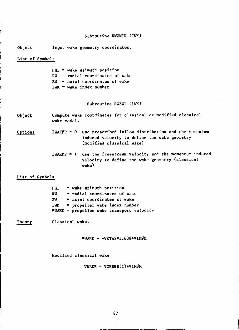
Subroutine RWZWIN (IWK)
Object Input wake geometry coordinates.
List of Svmbols
PHI = wake azimuth position RW = radial coordinates of wake ZW = axial coordinates of wake IWK = wake index number
Subroutine RWZWl (IWK)
Object Compute wake coordinates for classical or modified classical wake model.
Opt ions IWAK0P 0 use prescribed inflow distribution and the momentum induced velocity to define the wake geometry (modified classical wake)
IWAKQP = 1 use the freestream velocity and the momentum induced velocity to define the wake geometry (classical wake)
List of Symbols
PHI = wake azimuth position RW = radial coordinates of wake ZW - axial coordinates of wake IWK propeller wake index number VWAKE = propeller wake transport velocity
Theory C 1 ass ical wake.
VWAKE = -VKTAS*1.688+VIMgM
Modified classical wake
v w m = VZERgB(I)+VIM@M
87

Subrout ine RWZW7 (IWK)
Object Compute gene ra l i zed wake geometry.
Opt ions I0PT = 0 l i n e a r f i t f o r wake geometry between t i p - f i l a m e n t and non-rolled up f i l a m e n t s outboard of t h e o u t e r s h e e t f i 1 ament
IBPT = 1 p a r a b o l i c f i t f o r f i l amen t s as noted above
L i s t of Symbols
PHI = wake azimuth p o s i t i o n RW = r a d i a l coord ina te s o f wake ZW = axial c o o r d i n a t e s of wake IWK = wake index number
Theory See r e f e r e n c e 1.
Function SBFUNC (X)
Object C a l c u l a t e v a l u e o f s p e c i a l func t ion .
Argument L i s t
X = s p e c i f i e d independent parameter SBFUNC = f u n c t i o n v a l u e f o r s p e c i f i e d X
Theory A s p e c i a l f u n c t i o n f o r t h e s t a l l bucket ( r e f e r e n c e 11) is t a b u l a t e d f o r i n t e r p o l a t i o n on t h e independent parameter X. Beyond t h e range o f t a b u l a t e d d a t a , t h e fo l lowing f u n c t i o n i s used.
SBFUNC = ex-2. 139
Subroutine SETMAT
Object Read from a d i s k i n a s p e c i f i e d o r d e r t h e geometr ic i n f luence c o e f f i c i e n t s and combine them on ano the r d i s k f o r t h e m a t r i x s o l u t i o n a lgo r i thm.
L i s t o f Symbols
NPRBP = number of p r o p e l l e r s LTBT ITgT = number of i n f low s t a t i o n s MSIZE = matrix row s i z e GCC = chordwise i n f l u e n c e c o e f f i c i e n t s OCN = normalwise i n f l u e n c e c o e f f i c i e n t s as = spanwise i n f l u e n c e c o e f f i c i e n t s
= number of p r o p e l l e r p o s i t i o n s

Subroutine SQLVEL
Object
Options
Theory
Object
Opt ions
Theory
Calculate required quantities associated with the propeller aerodynamics and control the linearized solution procedure. flow diagram is presented in figure 14.
A
IDEBUG t: 0 print out intermediate quantities NEVARD f 0 ICAS f 0 use cascade airfoil data inboard of requested radial
IPRMAT f 0 MATSQL = 0 use direct matrix solution technique MATSQL 1 use iteration matrix solution technique LNF'T f 0 print circulation solution
use Evvard Tip Relief Correction
stat ion print matrix related quantities
See section entitled: "Linearized Aerodynamics" of reference 1.
Subroutine SgLVEN
Calculate required quantities for propeller aerodynamics and control the nonlinear matrix solution procedure. A flow diagram is presented in figure 15.
ICAS f 0 use cascade airfoil data inboard of requested radial
IPNT f 0 print intermediate circulation solutions MATSQL = 0 use direct matrix solution technique MATSQL = 1 use iterative matrix solution technique IDEBUG f 0 print out intermediate quantities
solution
See section entitled: "Nonlinear Aerodynamics" of reference 1.
89

Subroutine SgLVIT
Object
Opt ions
Control flow of solution procedure.
ITYPES = 0 linear aerodynamic solution only ITYPES = 1 nonlinear aerodynamic solution
Subroutine SPLLN3 (Argument List)
Object Interpolate using spline fit.
Options NW0T = controls calculation of derivatives
Argument List
XDATA YDATA NDATA XIN YQUT YPRIME NXY NW0T
= independent interpolation variable vector = dependent interpolation variable vector = number of interpolation table data points = vector of requested interpolation table data points = interpolation values at the interpolation points = vector of derivatives at the interpolation points = number of requested interpolation points = option control on derivatives
Theorv Standard spline fitting technique.
Subroutine STARC (Argument List)
Object Convert design lift coefficient to equivalent camber angle.
Argument List
DECL = design lift coefficient THSTAR = effective camber angle
Theory Using second order interpolation technique on a prestored table of data, the design lift coefficient is conwerted to the equivalent camber angle for a double circular arc airfoil.
90

Subroutine STQRE (I, J ,K ,X ,Y)
Object Store the vector X into the vector Y where X and Y can be externally dimensioned as three dimensional arrays.
Argument List
L , J , K = dimension limits of the X and Y arrays X = input vector (array) Y = output vector (array)
Function SWPCQIR (S , C0 ,MACH ,LAMLE ,LAMTE ,Y
Object Calculate tip loss factor for propeller blade using conical flow theory.
Argument List
S = semispan of wing which is used to approximate swept
CQI MACH = Mach number LAMLE = leading edge sweep angle LAMTE = trailing edge sweep angle Y = spanwise position on wing measured from midspan SWPCgR = scaling result
propeller tip = midspan chord of wing
Theory Concial flow theory for a thin sweep wing with subsonic leading edge and supersonic trailing edge is used to obtain the three- dimensional section C Q . equivalent thin wing two-dimensional solution t o obtain a scaling function t o apply to actual two-dimensional tabulated Cg data.
This solution is divided by the
91

Subroutine THlTER
Control selection of C or 5 blade angle iteration. P Object
Subroutine TITER (N,T,DQDT,QWANT,QCALC,T@L, IQ0K)
Object Linearly interpolate or extrapolate on input vector to obtain required T at requested Q.
Argument List
N = iteration index T = output vector DQDT = initially assumed slope of Q versus T curve QWANT = requested Q QCALC = input Q vector T0L = tolerance or solution IQ@K = iteration control flag
Subroutine UNBAR (Argument List)
Object Bivariant Interpolation on data vector.
Argument List
T IK = starting location of data XIN requested interpolation point ( X ) YIN requested interpolation point (Y) ZZ = interpolated value KK = interpolation flag
= table of bivariant interpolation data (2 vs. X and Y>
Theory Use standard bivariant interpolation algorithm with degree choice internally coded.
92

Subroutine UNINT (Argument List)
Object Univariant interpolation.
Argument List
I Theory I
NW = print output file number N = number of interpolation data points XA = vector of independent interpolation data YA = vector of dependent interpolation data X = requested interpolation point Y = resulting interpolated data values Z = interpolation flag
Interpolates over a four point interval using a variation of a 2nd degree interpolation to produce a continuity of slope between adjacent intervals.
Subroutine VECTQR
Object I I
Compute velocity related quantities required for propeller aero- dynamics.
ODtions
Theorv
Object 1
Opt ions
, Theory r
IDEBUG # 0 printout of selected intermediate quantities
Using vector algebra, the direction cosines of the local velocity vectors at the blade are calculated neglecting induced velocity terms, along with other related quantities.
Subroutine VVECTR
Compute velocity related quantities for the propeller aero- dynamics.
IDEBUG = 0 printout intermediate quantities.
Using vector algebra, the direction cosines of the local velocity vectors at the blade are compiled including effects along with other related velocity quantities.
93
i

Obiect Read wake displacement corrections from disk and modify the - internally calculated wake geometry.
Opt ions IDEBUG f 0 printout selected quantities
List of Symbols
PHI = wake azimuth position RW = radial wake coordinate zw = axial wake coordinate KT0T = number of wake filaments per blade NTQT = number of wake revolutions JTBT JTQTl = JTQT+l IDEBUG = print option
= number of wake azimuth positions per wake revolution
Theory See section entitled: Nacelle Influence on Wake Geometry of reference 1.
Subroutine WRITGC (Argument List)
Object Convert vectors of geometric influence coefficients to the blade coordinate system in the order in which they are calculated and write them to disk for later retrieval.
Opt ions IPRMAT f 0 printout geometric influence coefficients
Argument List
IX = local blade station index specifying the particular blade element station to transform the influence coefficients vectors from cylindrical to blade element coordinate system
LL t propeller position index IWK = propeller wake index IBB = blade index IP = propeller index IWRITE = disk number to write influence coefficients onto
Theory Standard geometric transformation applied to the cylindrical coordinate system influence coefficients to transform them to blade element coordinate system, before storing the disk for later retrieval.
94
,- ? i - d-

Subroutine ZERQGC (MK,NP ,N3 ,GC)
Object Set an externally dimensioned three dimensional array to zero.
Argument List
MK,N2,N3 = external dimensions of array GC GC = input array
Subroutine ZERQAL (THSTAR,APZL)
Object Calculate angle of zero lift for isolated airfoils.
Argument List
THSTAR = effective camber angle A~zL = angle of zero lift
Theory The angle of zero lift is calculated for the requested isolated airfoil type by computing the linear lift curve slope near zero angle of attack and solving for the intercept of the straight line with the resultant linear lift curve slope.
95

Labeled Common Blocks used in the Propeller Portion
Included herein is a list of the labeled common blocks in alphabetical order used in the propeller portion of the analysis and a description of each variable used in them (NDN designates a non-dimensional number).
Variable Common Block Name (Object) Names Description of Variables
AERDAT (Store Miscellaneous Aerodynamic Quantities)
AA
D LAG
CQNST
CMACH S MACH
CFDP
SKEW
Linearized lift curve slope
Diagonal element vector of (per radian)
geometric influence coefficient matrix (per ft.)
Constant vector of circulation solution matrix (ft2/sec)
Local total Mach number (NDN) Local section Mach number (NDN,
Constant vector correct ion term
Aerodynamic skew angle (degrees)
normal to lifting line)
( ft 2/sec)
AFDATX (Store Isolated Airfoil Data Package Quantities)
I I FL IDL ICASDE ALPHA THET TAUB ZM DECL H0B ZMCROM CL2 cL3 CD DCDCL
Inflow station index Airfoil type flag CL, CD calculation flag Cascade correction flag Local angle of attack (degrees) Local blade angles (degrees) Chord-to-gap ratio (NDN) Local Mach number (NDN) Design lift coefficient (NDN) Thickness-to-chord ratio (NDN) Critical Mach number (NDN) Lift coefficient (NDN) Temporary lift coefficient (NDN) Drag coefficient (NDN) Change in drag coefficient with
lift coefficient (NDN)
96

V a r i ab le Common Block Name Names Desc r ip t ion of Var i ab le s
BIGMAT (Large S to rage Matr ix , used p r imar i ly f o r wake geometry and ma t r ix c o e f f i c i e n t s t o r a g e )
PHI Wake segment azimuth ang le s (degrees)
C ~ S P H I Cosine of wake azimuth angles SINPHI Sine of wake azimuth angles RW Radial coord ina te of wake
zw Axial coord ina te of wake segments (NDN)
segments (NDN)
CASDT ( S t o r e Cascade and A i r f o i l Related Data)
S IGMAX Sec t ion cascade s o l i d i t y , gap- to-chord r a t i o (NDN)
THETAG Geometric angle between s e c t i o n chordwise vec to r and r o t a t i o n plane (degrees)
neg lec t ing induced terms (degrees)
THETAB Sec t ion angle of a t t a c k
TAUB Sec t ion chord-to-gap r a t i o (NDN)
CDPER ( S t o r e Nace l l e Drag Q u a n t i t i e s )
DFR DP R
Nace l le sk in f r i c t i o n drag ( l b ) Nace l le p r e s s u r e drag ( l b )
CCaM ( S t o r e S e c t i o n Chord Data)
CHQRD Blade element s e c t i o n chord
ALCRAD Blade element s e c t i o n chord l eng th ( f e e t )
l ength r a d i a l d i r e c t i o n cos ine (NDN)
ALCPHL Blade element s e c t i o n chord length t a n g e n t i a l d i r e c t i o n cos ine (NDN)
l eng th a x i a l d i r e c t i o n cos ine ALCAXL Blade element s e c t i o n chord
(NDN)
97

Var iab le Common Block Name Names Desc r ip t ion of Var i ab le s
CINC8M ( S t o r e Input Chord Data)
CINPUT Input chord length ( f e e t )
CLCDDT (S to re C i r c u l a t i o n S o l u t i o n and A i r f o i l C h a r a c t e r i s t i c s )
CLSAV Sec t ion l i f t c o e f f i c i e n t (NDN) CDSAV Sec t ion drag c o e f f i c i e n t (NDN) ALPHA S e c t i o n angle of a t t a c k
(degrees) PHINSD Sec t ion inf low angle (deg rees )
Sec t ion minimum drag c o e f f i c i e n t CDO
(NDN) CLRC S e c t i o n c i r c u l a t i o n ( f t Z / s e c ) SAVG I R Sec t ion ci :cculat ion from
FTRAN Interpolation function (NDN) previous i t e r a t i o n ( f t Z / s e c >
CONSTI ( S t o r e Input Data)
R P M
SQUND DENSTY VIMgM BL
R STN THETA0 WBQ DPSL
REV CP I
TQL CNSECT
SCQ RADCAS
P r o p e l l e r r o t a t i o n a l v e l o c i t y
Frees t ream speed of sound ( f p s ) Frees t ream d e n s i t y ( s l u g s / f t 3 > Momentum induced v e l o c i t y ( f p s ) Number of p r o p e l l e r b lades per
Blade r a d i u s ( f e e t ) Number of inf low s t a t i o n s Blade angle (degrees) Hub torque ( f t - l b f ) Blade azimuth increment
Number of wake r e v o l u t i o n s Requested power c o e f f i c i e n t
Matrix s o l u t i o n t o l e r a n c e (NDN) F r a c t i o n of b lade chord measured
Not used Blade r a d i u s denot ing t h e end of
( rmp)
p r o p e l l e r
(deg rees )
(NDN)
from l ead ing edge (NDN)
t h e cascade reg ion (NDN)
98

Variab le Common Block Name Names
VQRC0R DCPDT
STACK
CTI
DCTDT
ZHUB VKTAS TIPM RDTRAN RPMREF
DPSIB
OMEGA
DTIME
CQNSTl ( S t o r e I n t e r n a l Cons tan ts )
P I RC R 4 P I 0N04PI
CQNSTP ( S t o r e Misce l laneous Q u a n t i t i e s )
D I A 0K7R ZMSQ
UAX Z J I Mu
Desc r ip t ion o f Var i ab le s
Vortex core (NDN) Change i n power c o e f f i c i e n t with
b lade angle (pe r degree) P o s i t i o n of l i f t i n g l i n e as a
f r a c t i o n of t he b lade chord measured from the leading edge (NDN)
(NDN) Requested t h r u s t c o e f f i c i e n t
Change i n t h r u s t c o e f f i c i e n t
Coaxial hub displacement (NDN) Freestream v e l o c i t y (kno t s ) Tip Mach number (NDN) I n t e r p o l a t i o n r a d i u s l i m i t (NDN) Reference rpm f o r s teady load
Blade spacing azimuth i n t e r v a l
P r o p e l l e r r o t a t i o n a l speed
P e r i o d i c blade/wake geometry
wi th b lade angle (pe r degree)
induced t w i s t (rpm)
(degrees
( r a d / s e c )
time i n t e r v a l ( s e c )
n n/180 ( r a d i a l degree) 4 n x blade r a d i u s ( f e e t ) 1/R4PI (pe r f t . )
P r o p e l l e r diameter ( f e e t ) P r o p e l l e r t i p speed ( f p s ) Frees t ream Mach number squared
Frees t ream v e l o c i t y ( f p s ) Freestream advance r a t io (NDN) Frees t ream v e l o c i t y / t i p speed
(NDN)
(NDN)
99

Variab le Common Block Name Name s
CgNST3 (S to re Input Option S c a l a r s )
PR0PMN
PRMAT PR0PT DEBUG P CHP LT WAKEQP WAKNAC
EVAAFUI
CAS CAD TYP CAS CBWAKE C$ FL0W TAUEXP
c0mRs
SKINQP
Desc r ip t ion of Var i ab le s
See descr ip t . ion f o r s c a l a r i npu t s
11
11
11
11
11
11
11
11
11
11
11
11
11
11
CPTHET ( S t o r e Performance Related Q u a n t i t i e s )
N C P Performance i t e r a t i o n counter ICPQK Performance i t e r a t i o n c o n t r o l
THETO Blade angle s t o r a g e vec to r
CPCALC Power c o e f f i c i e n t s t o r a g e vec tor
CTCALC Thrus t c o e f f i c i e n t s t o r a g e
f l a g
( degrees 1
(NDN)
vec to r (NDN)
FCQM ( S t o r e Force Data)
FTQT
ALFRAD
ALFPHI
ALFAXL
T o t a l fo rce p e r u n i t a r e a ( l b f / f t 2 )
T o t a l fo rce p e r u n i t a r e a r a d i a l d i r e c t i o n cos ine (NDN)
T o t a l fo rce per u n i t a r e a t a n g e n t i a l d i r e c t i o n cos ine
T o t a l fo rce pe r u n i t a r e a a x i a l ( NDN 1
d i r e c t i o n cos ine (NDN)
100

Common Block Name Var i ab le
Names
FLTQT
ALFLRD
ALFLPH
ALFAX
FDTQT
ALFDRD
ALFDPH
ALFDAX
DescriDtion of V a r i a b l e s
L i f t fo rce per u n i t a r e a ( I b f / f t 2 >
L i f t fo rce per u n i t a r e a r a d i a l d i r e c t i o n cos ine (NDN)
L i f t fo rce per u n i t a r e a t a n g e n t i a l d i r e c t i o n cos ine
L i f t fo rce per u n i t a r e a a x i a l d i r e c t i o n cos ine (NDN)
Drag fo rce per u n i t a r e a (Hef/ f t 2,
Drag fo rce per u n i t a r e a r a d i a l d i r e c t i o n cos ine (NDN)
Drag fo rce per u n i t area t a n g e n t i a l d i r e c t i o n cos ine
Drag fo rce per u n i t a r ea a x i a l
( NDN )
( NDN 1
d i r e c t i o n cos ine (NDN)
FLIGHT ( S t o r e Frees t ream Q u a n t i t i e s )
ZMO Local s t a t i o n r o t a t i o n a l Mach
Z J O Local s t a t i o n advance r a t i o number (NDN)
(NDN)
FLPWDT ( S t o r e Inf low D i s t r i b u t i o n Data)
DENS Sec t ion d e n s i t y r a t i o (NDN) SgUN Sec t ion speed of sound ratio
VQNVO Sec t ion axial inf low v e l o c i t y r a t i o (NDN)
URQNVO Sec t ion r a d i a l in f low v e l o c i t y r a t i o (NDN)
V ZE R0 S e c t i o n c e n t e r a x i a l in f low v e l o c i t y ( f p s )
VZER0B S e c t i o n boundary axial inflow v e l o c i t y ( f p s )
( NDN 1
GCDIMD ( S t o r e Geometric I n f l u e n c e C o e f f i c i e n t s )
GCDIM Radia l , t a n g e n t i a l and a x i a l geometric i n f luence c o e f f i c i e n t s ( p e r f t )
101

Var i ab 1 e Common Block Name Names Desc r ip t ion of Var i ab le s
GCKDAT ( S t o r e ind iv idua l t r a i l i n g f i lament and bound vor t ex i n f l u e n c e c o e f f i c i e n t s )
GCKRTZ Radia l , t a n g e n t i a l and a x i a l t r a i l i n g vo r t ex f i lament i n f luencc: c o e f f i c i e n t s
bound vor t ex in f luence c o e f f i c i e n t s
GCRTZB Rad ia l , t a n g e n t i a l and ax ia l
GEQDAT ( S t o r e Blade Geometry Q u a n t i t i e s )
RSB
ZSB
YSB
RSBB ZSBB
YSBB
PHIBB
RSC
RSCC
zscc
PHICC
XSBB
xscc
COSLB
SINLB
Input x-wise segment boundary
Input a x i a l segment boundary
Input y-wise segment boundary
Segment boundary r a d i u s (NDN) Segment boundary droop ( a x i a l )
d is p 1 acement ( NDN) Segment boundary 1 ag
displacement (NDN Segment boundary l ag ang le
(degrees Input segment c e n t e r r a d i a l
coord ina te (NDN) Inpu t segment c e n t e r r a d i a l
coord ina te (NDN) a f t e r b lade angle r o t a t i o n
d i s p 1 acement ( NDN) a f t e r b 1 ad e angle r o t a t i o n
displacement (NDN) a f t e r b lade angle r o t a t i on
(deg rees )
coord ina te (NDN)
coord ina te (NDN)
coord ina te (NDN)
Input segment c e n t e r axial
Input segment c e n t e r l a g
Input segment c e n t e r l ag angle
Segment boundary x-wise l o c a t i on
Segment cen te r x-wise l o c a t i o n
Cosine of b lade segment boundary
S ine of b lade segment boundary
(NDN)
(NDN)
l ag angle
l a g angle
102

Var iab le Common Block Name Names
GEQINP ( S t o r e Inpu t I n t e r p o l a t i o n Arrays)
v0Nv0x
cx DTHETX
TQVERX
BETAB
BETAC
GEQMgD ( S t o r e Design L i f t C o e f f i c i e n t )
DESCLP
GEQQUT ( S t o r e Blade S e c t i o n P r o p e r t i e s )
DTHETA
AFQ I L DESCL
TQVERC
103
DescriDtion o f V a r i a b l e s
Axial inf low r a t i o d i s t r i b u t i o n
Input chord d i s t r i b u t i o n ( f e e t ) Input p i t c h angle d i s t r i b u t i o n
(deg rees ) Input thickness-to-chord r a t i o
d i s t r i b u t i o n (NDN) Load induced t w i s t increment a t
b l ade segment boundary p o i n t s (degrees)
Load induced t w i s t increment at b lade segment boundary p o i n t s (degrees
(NDN)
Sec t ion des ign l i f t c o e f f i c i e n t (NDN)
Input section p i t c h ang le
Sec t ion a i r f o i l type (NDN) Input sec t ion des ign l i f t
Sect i on thickness-to-chord rat i o
Sect i on chord-to-diameter ra t i o
(deg rees )
c o e f f i c i e n t s (NDN)
(NDN)
(NDN)

Var iab le Common Block Name Names Desc r ip t ion of Var i ab le s
G4OODT ( S t o r e Q u a n t i t i e s from Aeroe la s t i c Response Analys is )
NG400 Option f l a g NSEG Number of blade s t a t i o n s i n the
XYZCG Segment center coord ina te s of response a n a l y s i s
b lade s t a t i o n s used i n t h e response a n a l y s i s
segment C R from t h e response a n a l y s i s
G400CD Quadra t ic c o e f f i c i e n t s f o r segment CD from the response a n a l y s i s
G400CL Quadra t ic c o e f f i c i e n t s f o r
IgUNIT ( S t o r e S tandard Input /Output Unit Numbers)
NREAD Standard input u n i t NWRITE Standard p r i n t u n i t NPUNCH Standard punch u n i t
INTDl S to re Indexing L i m i t s )
LT0T KTQT
JTQT NREX
NBLggP LTQT NPRQP MTQT MS I ZE NBCALC IFL
Number of inf low s t a t i o n s Number of inf low s t a t i o n
Number of blade azimuth s t a t i o n s Number of r e v o l u t i o n s of wake
Number of b lade loops Number of p r o p e l l e r p o s i t i o n s Number of p r o p e l l e r s Number of segment endpoin ts LTQ T*JTQ T*JT$T Number of b lade c a l c u l a t i o n s A i r f o i l type index v e c t o r
boundaries
ge ome t r y
104
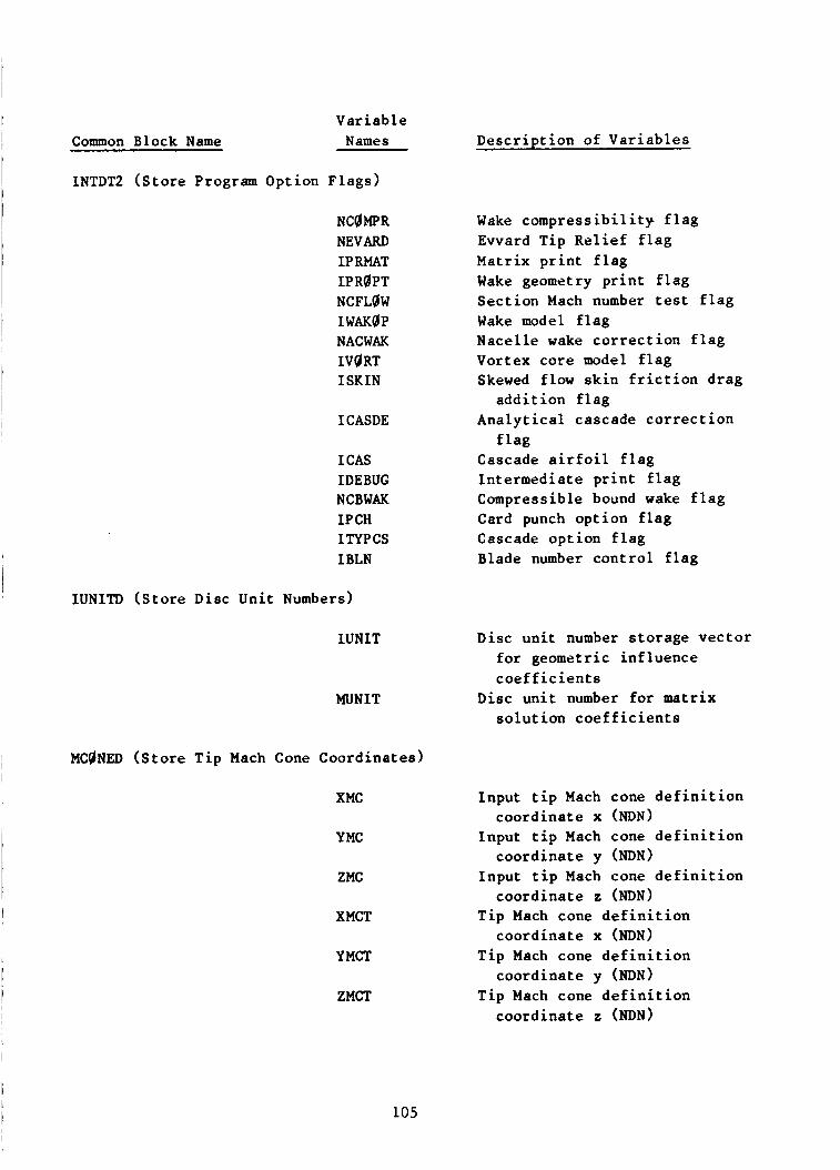
Common Block Name
INTDTP (Store Program Opt
V ar iab 1 e Names
on Flags)
NCQMPR NEVARD IPRMAT IPRgPT NCFLQW
NACWAK
ISKIN
IWAKQP
IVQRT
I CASDE
ICAS IDEBUG NCBWAK IP CH LTYPCS I BLN
IUNITD (Store Disc Unit Numbers)
LUNIT
MUNIT
MCQNED (Store Tip Mach Cone Coordinates)
XMC
YMC
ZMC
XMCT
YMCT
ZMCT
Description of Variables
Wake compressibility flag Evvard Tip Relief flag Matrix print flag Wake geometry print flag Sect ion Mach number test flag Wake model flag Nacelle wake correction flag Vortex core model flag Skewed flow skin friction drag
Analytical cascade correction
Cascade airfoil flag Intermediate print flag Compressible bound wake flag Card punch option flag Cascade option flag Blade number control flag
addition flag
flag
Disc unit number storage vector for geometric influence coefficients
Disc unit number for matrix solution coefficients
Input tip Mach cone definition
Input tip Mach cone definition
Input tip Mach cone definition
Tip Mach cone definition
Tip Mach cone definition
Tip Mach cone definition
coordinate x (NDN)
coordinate y (NDN)
coordinate z (NDN)
coordinate x (NDN)
coordinate y (NDN)
coordinate z (NDN)
105
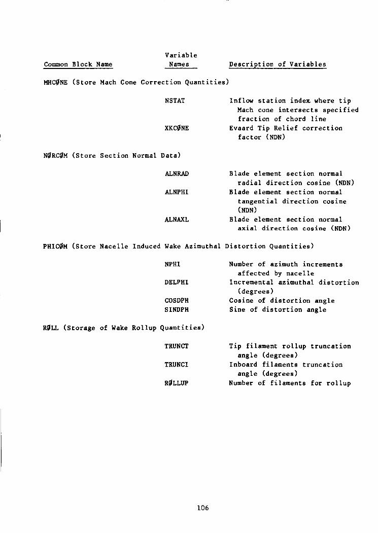
Var i a b 1 e Common Block Name Names Desc r ip t ion of V a r i a b l e s
MHCQNE ( S t o r e Mach Cone Cor rec t ion Q u a n t i t i e s )
NSTAT
XKCgNE
Inflow s t a t i o n index where t i p Mach cone i n t e r s e c t s s p e c i f i e d f r a c t i o n of chord 1 i n e
f a c t o r (NDN) Evaard Tip Re l i e f c o r r e c t i o n
N0RC0M ( S t o r e S e c t i o n Normal Data)
ALNRAD Blade element s e c t i o n normal
ALNPHI Blade element s e c t i o n normal r a d i a l d i r e c t i on cos ine (NDN)
t a n g e n t i a l d i r e c t i o n cos ine (NDN)
ALNAXL Blade element s e c t i o n normal a x i a l d i r e c t i o n cos ine (NDN)
PHICOM ( S t o r e Nace l l e Induced Wake Azimuthal D i s t o r t i o n Q u a n t i t i e s )
NPHI Number of azimuth increments
DELPHI Incrementa l azimuthal d i s t o r t i o n
COSDPH Cosine of d i s t o r t i o n ang le SINDPH Sine of d i s t o r t i o n angle
a f f e c t e d by n a c e l l e
(deg rees )
ROLL (S to rage of Wake Rol lup Q u a n t i t i e s )
TRUNCI' T i p f i lament r o l lup t runca t ion
TRUNCI Inboard f i l amen t s t r u n c a t i o n
RgLLUP Number of f i l amen t s f o r r o l l u p
ang le (deg rees )
angle (degrees)
106
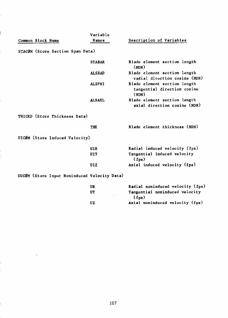
Var iab le Common Block N a m e Names
STAC0M ( S t o r e S e c t i o n Span Data)
STABAR
ALSRAD
ALSPHI
ALSAXL
Desc r ip t ion of V a r i a b l e s
Blade element s e c t i o n l eng th
Blade element s e c t i o n l eng th
Blade element s e c t i o n l eng th
(NDN)
r a d i a l d i r e c t i o n cos ine (NDN)
t a n g e n t i a l d i r e c t i o n cos ine ( NDN 1
Blade element s e c t i o n l eng th a x i a l d i r e c t i o n cos ine (NDN)
T H I O ( S t o r e Thickness Data)
THK Blade element t h i ckness (NDN)
U I C a M ( S t o r e Induced V e l o c i t y )
U I R UIT
U I Z
UUCQH ( S t o r e Input Noninduced Ve loc i ty Data)
Radia l induced v e l o c i t y ( f p s ) Tangen t i a l induced v e l o c i t y
Axial induced v e l o c i t y ( f p s ) ( f p s )
UR UT Tangen t i a l noninduced v e l o c i t y
uz Axial noninduced v e l o c i t y (fps)
Radia l noninduced v e l o c i t y ( f p s )
( f p s )
107

Vat i a b l e Common Block Name Names
VC8M ( S t o r e Noninduced Ve loc i ty Data)
ALP"
vs
vc
VN
VTQT ALVRAD
ALVPHI
ALVAXL
VIDAT ( S t o r e Induced Ve loc i ty )
VIS V I C V I N
WAKDAT ( S t o r e Wake Rollup Data)
KTRUCT
JTRUCT
JTRUCI
Desc r ip t ion of V a r i a b l e s
Noninduced angle of -at t a c k ( r a d i a n s )
Spanwise noninduced v e l o c i t y d i r e c t i o n cos ine (NDN)
Chordwise noninduced v e l o c i t y d i r e c t i o n cos ine (NDN)
Normalwise noninduced v e l o c i t y d i r e c t i o n cos ine (NDN)
T o t a l noninduced v e l o c i t y ( f p s ) Radia l noninduced v e l o c i t y
d i r e c t i o n cos ine (NDN) Tangen t i a l noninduced v e l o c i t y
d i r ec t io r i cos ine (NDN) Axial noninduced v e l o c i t y
d i r e c t i o n cos ine (NDN)
Spanwise induced v e l o c i t y ( f p s ) Chordwise induced v e l o c i t y ( f p s ) Normalwise induced v e l o c i t y
( f p s )
Fi lament s t a t i o n index f o r
Wake azimuth p o s i t i o n index f o r
Wake azimuth p o s i t i o n index f o r
r o l l u p
t i p r o l l u p
roo t r o l l u p
108

I Nacelle Program
I I A detailed description of the nacelle portion of the computer program is
given in this section. individually in alphabetical order. The labeled common blocks are briefly described along with the FORTRAN variables used in them. Flow charts and figures are provided whenever necessary to understand the objectives and theory for the subroutines or external functions.
The subroutines and external functions are described I I I
1 109

List of Subroutines and External Functions
Name - Object
ALTMN Control 1/0 and calculation flow
AMF Compute isentropic nozzle flow
AMFLQI Calculate Mach number f r m area ratio
AMU Compute molecular viscosity
BATCH
BILINE
BLDGEO
BLDQUT
Main routine
Calculate neighboring points on output line
Locate blade centerline
Store blade parameters on drum
BLKDAT Load block data
BLKRED Read data records from mass storage device
BLPARM Compute boundary layer parameters
BPLUSR Compute law of wall integration constant
CALDRM Read inviscid or viscous solution from drum
CALINV Calculate inviscid flow field
CDS Calculate Roberts' mesh distortion parameter
CKINPT Check input data for radial equilibrium
C0gR Interpolate coordinates
C0@ RST Control flow of coordinate calculation
Cg0Rl Compute approximate coordinates
C00U Compute coordinate functions
C00R4 Compute Schwartz-Christoffel parameters
ce0Rs Interpolate wall curvature at station 5
CPLXl Evaluate Schwartz-Christoffel transform
DAMU Find derivati *e of molecular viscosity
110
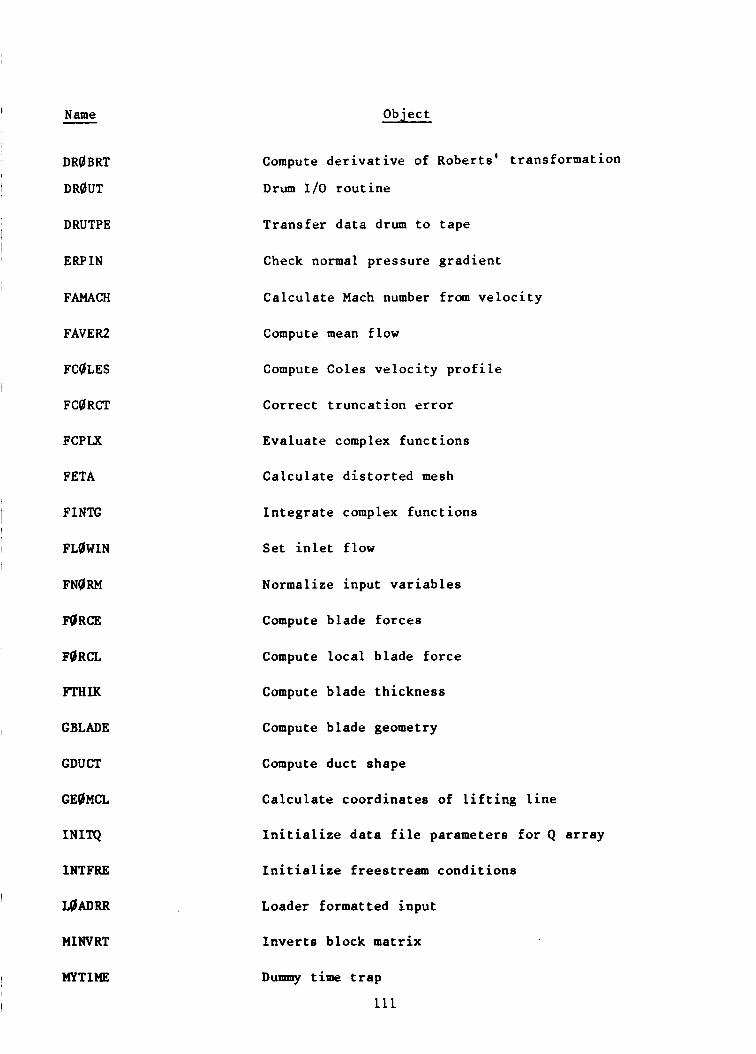
Name I -
D R ~ B R T
I DRgUT
I DRUTPE
I ERP I N
FAMACH
FAVER2
FCgLES
FCQRCT
FCPLX
FETA
I F I N E I I
I FLQWIN
FNg RM
Fd RCE
FQRCL
FTHIK
I GBLADE
GDUCT
GEQHCL
I N I T Q
INTFRE
L O R R I
MINVRT
1 MYTIME
Object
Compute d e r i v a t i v e of
D r u m L/O r o u t i n e
T r a n s f e r d a t a drum t o
Check normal p re s su re
C a l c u l a t e Mach number
Compute mean f low
Roberts ' t r ans fo rma t ion
t a p e
g r a d i e n t
from v e l o c i t y
Compute Coles v e l o c i t y p r o f i l e
Correc t t r u n c a t i o n e r r o r
Eva lua te complex func t ions
C a l c u l a t e d i s t o r t e d mesh
I n t e g r a t e complex func t ions
S e t i n l e t f low
Normalize input v a r i a b l e s
Compute b lade f o r c e s
Compute l o c a l b l ade f o r c e
Compute b lade t h i c k n e s s
Compute b lade geometry
Compute duc t shape
C a l c u l a t e coord ina te s of l i f t i n g l i n e
I n i t i a l i z e d a t a f i l e parameters f o r Q a r r a y
I n i t i a l i z e f r ees t r eam c o n d i t i o n s
Loader formatted inpu t
Lnver t s block matrix
Durnmy time t r a p
111

Object
P r i n t t i t l e page
Name - PUTPUT
Compute v iscous n a c e l l e d rag PERFNA
Compute i n v i s c i d n a c e l l e d rag PERFNP
P0IS Solve Poisson equa t ion
PdISCF S e t i n i t i a l q u a n t i t i e s in s o l u t i a a procedure
PO I S0N C a l c u l a t e axisymmetric s t r eaml ine c u r v a t u r e
QINTER I n t e r p o l a t e cu rva tu re
Read P and F f i l e s READPF
READPG
RQBRTS
Read v a r i a b l e f o r cu rva tu re c a l c u l a t i o n
Compute d i s t o r t e d mesh us ing Roberts ' t r ans fo rma t ion
Round co rne r s on s t r a i g h t w a l l d u c t s ROUND
C a l c u l a t e cu rva tu re from p o t e n t i a l flow s o l u t i o n S CURVA
SLETE Find blade c o n t r o l s u r f a c e s
Smooth duct wall contour
NLVI SPLIN3
I n t e g r a t e equat ions of s t a t e
NASA S p l i n e F i t r o u t i n e
Compute i n i t i a l stress d i s t r i b u t i o n s STRESI
Find i n l e t f low l o c a t i o n s STRT
Ca l l CPU t i m e TP RLNT
Compute t u r b u l e n t v i s c o s i t y TURB
UBLAS Calculate v e l o c i t y r a t i o according; t o B l a s i u s s o l u t i o n
Compute Coles f r i c t i o n veloci ty U C ~ L E S
WAKC$R Compute n a c e l l e wake c o r r e c t i o n s
112

I Name - WBLEED
WRITPF
XH
XT
. Object
Ca lcu la t e pe r fo ra t ed wall b leed
S t o r e updated p o t e n t i a l flow s o l u t i o n
C a l c u l a t e w a l l l ength on I D wal l
C a l c u l a t e w a l l l eng th on OD wall
Descr -p t ion of Su-rout ines and Ex te rna l Funct ions
Th i s s e c t i o n d e s c r i b e s t h e sub rou t ines and e x t e r n a l func t ions used i n t h e n a c e l l e po r t ion of the a n a l y s i s . The source name f o r t he main c o n t r o l r o u t i n e is c a l l e d BATCH and has the fol lowing two e n t r y po in t s : ALTMN and QFFLNE. The main program determines the e n t r y point ALTMN o r 0FFLNE.
113
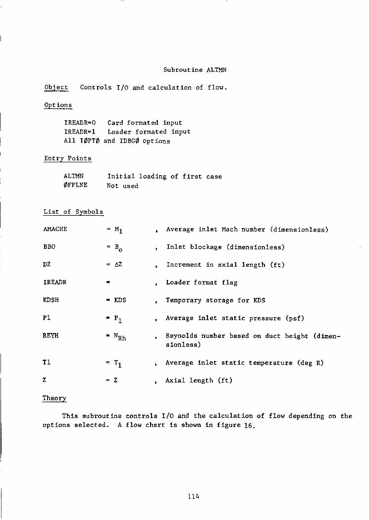
Subrout ine ALTMN
Object Cont ro ls I / O and c a l c u l a t i o n of f low.
Options
IREADR=O Card formated input IREADR=l Loader formated inpu t A l l IBPTb and IDBGB o p t i o n s
Entry P o i n t s
ALTMN I n i t i a l loading of f i r s t ca se 0FFLNE Not used
L i s t of Symbols
AMACHE = Mi 9
BBO = Bo 7
DZ = AZ 9
IREADR - - 7
KDSH = KDS 9
P1 = P1 9
REYH = NRh 7
T1 = T1 9
2 = z 9
Theory
Average i n l e t Mach number (d imens ionless )
I n 1 et b l o c kag e ( d imen s ion 1 e s s )
Increment i n a x i a l l e n g t h ( f t )
Loader format f l a g
Temporary s t o r a g e f o r KDS
Average i n l e t s t a t i c p r e s s u r e ( p s f )
Reynolds number based on duc t he igh t (dimen- s ion1 es s )
Average i n l e t s t a t i c tempera ture (deg R)
Axia l l e n g t h ( f t )
Th i s sub rou t ine c o n t r o l s 1/0 and t h e c a l c u l a t i o n of f low depending on t h e o p t i o n s s e l e c t e d . A f low c h a r t i s shown i n f i g u r e 16.
114

Subrout ine AMF(AA,AMl,AMG,AM,ACPC,ACPI)
Object Compute i s e n t r o p i c n o z z l e flow
Opt ions
AMG < 1 Subsonic s o l u t i o n ANG > 1 Supersonic s o l u t i o n
L i s t of Symbols
AA = A/A1
V AAI = ( A / A ~ )
ACPC = cp
ACP I = CpI
AM = M
V AMI = M2
AM1
AP2
AP2
c1
c2
c 3
c4
c5
= M1
= Po/P1
= P0/P2
= y-1/2
= 1 Y + 1 2 y-1 - -
7
7
7
7
7
7
7
7
7
7
7
Area r a t i o
vth guess f o r area r a t i o
P r e s s u r e c o e f f i c i e n t
Incompress ib le p r e s s u r e c o e f f i c i e n t
Mach number
Funct ion name
1st guess f o r Mach number
Vth guess f o r Mach number
Mach number a t s t a t i o n 1
S t a t i c p r e s s u r e a t s t a t i o n 1
S t a t i c p r e s s u r e a t s t a t i o n 2
= (Y+U
Cons tan ts i n I t e r a t i o n
115

C6
c7
= Y I Y - 1
Y - 1 Cons tan ts i n I t e r a t i o n - (1 + 2 ) -
DAAI = (dA/dM)' , D e r i v a t i v e
DAM1 = A M , Correc t ion t o Mach number
ITER = v , I t e r a t i o n coun te r
Theory
Fiven t h e area r a t i o A/A1 and t h e i n l e t Mach number M1, f i n d t h e e x i t Mach number M, ' the p r e s s u r e c o e f f i c i e n t Cp , and t h e incompress ib le c o e f f i c i e n t
CpI. The e x i t Mach number M is determined from t h e one-6imensional i s e n t r o p i c f low r e l a t i o n s us ing Newton's method f o r determining r o o t s of n o n l i n e a r equa- t i o n s . Thus, w e s e t u p t h e i t e r a t i o n c y c l e
When I AMI < be computed.
t h e i t e r a t i o n has converged and t h e p r e s s u r e c o e f f i c i e n t may
116

Subroutine AMFLd (AA, AMl, AMG, AM, ACPC, ACPI)
Object Calculate Mach number from area ratio
Variables
AA A/A Area ratio
Compressible pressure coefficient cPc ACP C
Incompressible pressure coefficient ACP I CPI
AM M Mach number
AMG Flag
Mach number at station 1 M1 AM1
Theory
The Mach number can be calculated from Y + l
2 Y-1 M2 1+-
(l++M;)
using Newton's iteration. With M known, 9 L
:: 1 - (4) cP*
Y - pT Y-1 - = [l + y M12] P1
Y-1 y - l 2 M I
pT 2
- =[1+ P
= ( + y ( l - < ) P P
cPc
AElG < Subsonic root of (1)
AMG > Supersonic root of (1)
117

Func t ion Iu?u (T)
Object Compute molecular v i s c o s i t y
Opt i ons
None
L i s t of Symbols
AMU = P I P r , Rat io of molecular v i s c o s i t y (d imens ionless )
T = 0 , S t a t i c tempera ture r a t i o (d imens ionless )
Theory
The molecular v i s c o s i t y is computed according t o Su the r l and ' s formula (Ref. 6 ) . The working f l u i d is assumed t o be a i r . Accordingly,
P 312 I + 198.0/Tr p; = o Q + 198.0/Tr
Subrout ine BLDgUT
Object Write ( o r r ead ) b l ade parameters on drum
Entry P o i n t s BLDIN BLLMUT
BLDQIUD BLDIND
BLDBK
L i s t of Sythbols
STRI, STR3, STRS, STR7, ISTR8 b lade parameters (dimensional)
STR2, STR4, STR6 b l a d e Parameters (nondimensional)
Theory
Blade parameters f o r each row of b l ades are s t o r e d on a drum. Th i s r o u t i n e w i l l r ead o r w r i t e on to t h a t drum.
118

Main Program BATCH
Obi e c t !la i n program
V a r i a b l e s None
T h e o z
The main programs ca l l s only s u b r o u t i n e s TITLE and ALTMN
119
i Subroutine BILINE (L,RB1,ZB1,RB2,Z8B2)
Calculate neighboring points on output line
I Options
None
Variables
I L ) Point number - -
RB1,ZBl = R1,Z1 , Point at L-1
- - RB2,ZB2 = R2)Z2 , Point at L
I Theory
The points are read from an input table.
120

Subrout ine BLDGEb
Object
Locate b l ade c e n t e r l i n e i n ( n , s > coord ina te s
O p t ions
IdPT2 = 0 No b lades i n duc t
= 1 Blades i n duc t
L i s t of Symbols
CbMMON BLBCK Var i ab le s
Theory
This s u b r o u t i n e uses sub rou t ine FLINE t o f i n d t h e c e n t e r l i n e i n t h e ( n , s > coord ina te s . Thus t h e i n p u t d a t a from t h e b l ade s t a c k i n g p l ane i s transformed t o t h e duc t p l a n e us ing s u b r o u t i n e TRBLD and s t o r e d i n t h e i n p u t d a t a l i n e d a t a block BLNE ( I , 2 ) used by s u b r o u t i n e FLINE. s t o r e d i n t h e b l a d e d a t a a r r a y CONST(1,L). t h e l o c a t i o n of t h e upstream and downstream b lade f o r c e c a l c u l a t i o n s u r f a c e s are determined by c a l l i n g s u b r o u t i n e SLETE.
The ou tpu t ( n , s ) coord ina te s a r e t h e n A t t h e completion of t h i s c a l c u l a t i o n ,
121

Subrout ine BLKDAT
Object Load f i x e d c o n s t a n t s t o program.
Opt i o n s
None
L i s t of Symbols
ACHI
AKAPPA
APLUS
CPR
CVR
EP
GAMMA
GASR
GRAVR
P I
PRESR
PRL
PRT
RH@R
SNDR
TEM'PR
T I
VISCR
= x = K
= A+
= Cpr
vr = c
= e
= Y
= R
= g
= T I
= P,
= 'rL
- P r t
= P r
-
= cr
= T,
= t
= P r
0.016 (d imens ionless )
0.41 (d imens ionless )
26.0 (d imens ionless )
5997. ( f t 2 / s e c 2 / d e g R)
4283. ( f t 2 / s e c 2 / d e g R)
2.7182818 (d imens ionless )
1 . 4 (d imens ionless )
1714. ( f t2 / sec2/deg R)
32.2 ( f t / s e c )
3.1415926
2117. ( f t 2 / s e c /deg R)
0.72 (d imens ionless )
0.90 (d imens ionless )
0.00238 ( s l u g s / f t 3 )
1116.0 ( f t / s e c )
519.0 (deg R)
0.01745329 (dimensionless:)
0.37 x ( s l u g / f t / s e c )
2
2
122

I Values of pa rame te r ' s d e f i n e d i n C@MM@N/PARAM/ are a l s o inc luded f o r
IBM and CDC computer programs. I
Subrout ine BLKRED (UNIT, R E C S I Z , ADDR, BEGREC, NRECS)
Object
Reads NREC ' r e c o r d s ' from f i l e ' U N I T ' beginning w i t h record BEGREC. NRECS r eco rds are s t o r e d as a s i n g l e b lock , beginning a t ADDR. 1/0 r o u t i n e NTRAN is used i n t h i s sub rou t ine .
The Univac 1100 l i b r a r y
Var i ab le s
U N I T = l o g i c a l u n i t # ( I n t e g e r ) RECSIZ = r eco rd s i z e i n words ( I n t e g e r ) BEGREC = f i r s t r eco rd t o read ( I n t e g e r ) NRECS = # of l o g i c a l r eco rds t o read ( I n t e g e r ) ADDR = beginning addres s t o s t o r e t h e NRECS & RECSIZ
r e c o r d s r ead
Theory
BLKRED (wi th e n t r y BLKWRT) was developed t o a l low NTRAN c o m p a t i b i l i t y w i t h ANSI I n p a r t i c u l a r , a c a l l t o BLKRED wi th NRECS = 1 s tanda rd DEFINE FILE 1/0 o p e r a t i o n s .
i s i d e n t i c a l t o a random a c c e s s f o r t r a n read .
I n o r d e r t o s i m u l a t e DEFINE FILE I / O , i t is necessa ry f o r BLKRED t o main ta in a l is t of p o i n t e r s i n t o t h e v a r i o u s d i s k f i l e s . The p o i n t e r l i s t , DSKLOC, i s i n a common b lock \ U N I T S / which must be a l l o c a t e d i n a s t a t i c ( r o o t ) segment. t i o n p o i n t e r and read s i z e are used t o p o s i t i o n t h e d i s k f o r 1 /0 access .
The loca- A f t e r t h e
I 1/0 access , t h e p o i n t e r i s pos i t i oned acco rd ing ly .
BLKRED w i l l i s s u e a d i a g n o s t i c message and cause program t e rmina t ion i f e i t h e r of two abnormal c o n d i t i o n s are d e t e c t e d .
1) t h e r eco rd II i s n e g a t i v e
2) NTRAN r e t u r n s on e r r o r s t a t u s less than ze ro (see UNIVAC FORTRAN V l i b r a r y r o u t i n e NTRAN d e s c r i p t i o n on UNIVAC ASCII FORTRAN r o u t i n e NTRANd d e s c r i p t i o n )
123

Subrout ine BLPARM
Object C a l c u l a t e boundary l a y e r parameters from viscocis s o l u t i o n .
Options I1 = 1 C a l c u l a t e hub boundary l a y e r I1 = 2 C a l c u l a t e t i p boundary l a y e r
L i s t of Symbols
BLC(1, I)
BLD(2, I)
= U Freestream v e l o c i t y
= n S t a t i c P r e s s u r e
m
BLP(3, I) = To T o t a l t empera ture
BLP(4, I) = T S t a t i c temperature
BLP(5, I) = M Mach number
BLP(6, I) = us Streamwise v e l o c i t y
BLP(7, I) = P Dens i t y
BLP(8, I) = Y D i s t a n c e from hub
BLP(9, I) = A*/A1 Displacement t h i c k n e s s r a t i o
BLP(10, I) = e*/el Momentum t h i c k n e s s r a t i o
BLP(11, I) = A*/8* Shape f a c t o r
BLP(12, I) = N e Reynolds number
CF = Cf Wall F r i c t i o n C o e f f i c i e n t
Theory
T h i s s u b r o u t i n e s determines t h e momentum t h i c k n e s s and t h e displacement
t h i c k n e s s A* where 8
124

Funct ion BPLUSR (AKPLUS)
1 I Object Compute t h e l a w of w a l l i n t e g r a t i o n cons t an t f o r i n i t i a l p r o f i l e .
Options None
None
L i s t of Symbols
AKPLUS +
, Roughness Reynolds number KS
BPLUSR B+ (K~+) , I n t e g r a t i o n cons t an t
Theory
The i n n e r l a y e r t u rbu lence model g iven i n FCOLES w a s i n t e g r a t e d t o g e t + + t h e cons t an t of i n t e g r a t i o n . A d a t a c o r r e l a t i o n f o r B (Ks ) is then g iven by
B+ (0) = 2.2 US< + 4.1270
B+ (KZ) = - 0.81486 - 1.2070 * (In K, - 3.91538) , K:>4.1270 (2)
+ Equat ion (1) i n d i c a t e s t h a t f o r K < 4.127, t h e smooth w a l l model a p p l i e s . S
Subrout ine CALDRM
Object Read i n v i s c i d o r v i scous s o l u t i o n from (drum)
Options
NgPT8 = 0 Read i n v i s c i d s o l u t i o n NgPT8 = 1 Read v i s c o u s s o l u t i o n
L i s t of Symbols
F Viscous flow parameters
CINP I n v i s c i d flow parameters
125

Subrout ine CALINV
Object C a l c u l a t e i n v i s c i d f low f i e l d s o l u t i o n .
Options
C a l c u l a t e flow from J = JFIRS, JLAS I F (IQPT15.NE.O) JFIRS=I@PT15 I F (IQPT16.HE. 0) JUS=I@PT16
Ca lcu la t e only f o r I0PTl = 3 o r 4 NOPTS # 0 Er ro r e x i t
L i s t of Symbols
Same as CKINPT
Var i ab le s t o r e on drum K = l , K L
BINP(1, K)
BINF'(2, K)
BINP(3, K)
BINP(4, K)
Add i t iona l V a r i a b l e s
ITERAL
ERRA
ERRAM
Theory
, T o t a l p r e s s u r e ( p s f )
P , S t a t i c p r e s s u r e ( p s f )
a , Swi r l a n g l e (deg)
, T o t a l tempera ture (deg R) TO
, Swi r l a n g l e i t e r a t i o n number
, Local e r r o r i n s w i r l a n g l e
a V
Ea
, Maximum e r r o r i n s w i r l ang le End
Given t h e s w i r l a n g l e a , t h e a n a l y s i s bs i d e n t i c a l t o s u b r o u t i n e CKINPT. of t h e angu la r momentum equa t ion which is g iven by
The c a l c u l a t i o n of t h e i n v i s c i d f low f i e l d r e q u i r e s a l s o t h e s o l u t i o n
where RU l e t angu la r momentum which i s given. grammed t o s o l v e e q t . (1) to g e t t h e s w i r l a n g l e a . i n n e r i t e r a t i o n loop is t h e same as s u b r o u t i n e CKINPT. ob ta ined f o r each streamwise s t a t i o n J = JFIRS, JLAS. BINP (4 , KL) is s t o r e d on a drum.
is t h e angu la r momentum a t an a r b i t r a r y s t a t i o n and R U is t h e in- ti dl An o u t e r i t e r a t i o n lciop is hen pro-
With a known, t h e Th i s s o l u t i o n is
The computed s o l u t i o n
126

Funct ion CDS (DDS, DETA)
Object
Ca lcu la t e Rober t s ' mesh d i s t o r t i o n parameter
Options
None
Input Var i ab le s
DDS =
DETA = 6q , An
Output Var i ab le s
CDS c 9
Theory
L e t
Ratio of mesh d i s t o r t i o n a t w a l l Aq/An
Mesh s i z e a t boundary - m i f o r m mesh D i s t o r t e d mesh s i z e a t w a l l
Rober t s ' mesh parameter
c = 1/2 + Q
Then Roberts ' t r ans fo rma t ion can be w r i t t e n
A n = A 7 / D D S
Eq. (2) through ( 4 ) can be solved i t e r a t i v e l y f o r E as fo l lows:
i = O
A n + € + = I+c-An
127
Subroutine CDS (Cont'd)
I Convergence occurs when
1
128

Subrout ine CKINPT
I
Object Check inpu t d a t a f o r r a d i a l e q u i l i b r i u n
Options ,
IQPTl # 4
N@PT5 # 0
I@PT5 = 2
IJ = 1
IB = 2
IMEX = 1
INEX = 2
IDBG13 = 1
!*[email protected] = 0
w n @ K > 0
L i s t of Symbols
ERR E.
EP S
FG(2, K) $(2)
FG(4, K) @(2)
ITER v
PHMAX
€0
v v PSI1 , PSI2 qJl , qJ2
WF WV2
WFLdbJ W
'max WMAX
Do no t c a l c u l a t e
E r r o r e x i t
FgRCE d a t a equa l s FLgWIN d a t a
I n l e t f low d a t a
Force d a t a
Upstream d a t a
Downstream d a t a
Debug p r i n t o u t
S t a t i c p r e s s u r e check only
P r e s s u r e check and weight f low i t e r a t i o n
9
9
9
9
9
9
9
9
9
9
E r r o r i n i n t e r a c t i o n
Minimum e r r o r
Equation 4
Equation 5
I t e r a t i o n number
Maximum p r e s s u r e p o s s i b l e
Upper and lower bound a i r stream f u n c t i o n
Weight f low vth i t e r a t i o n
Input weight f low
Maximum weight f low p o s s i b l e
129
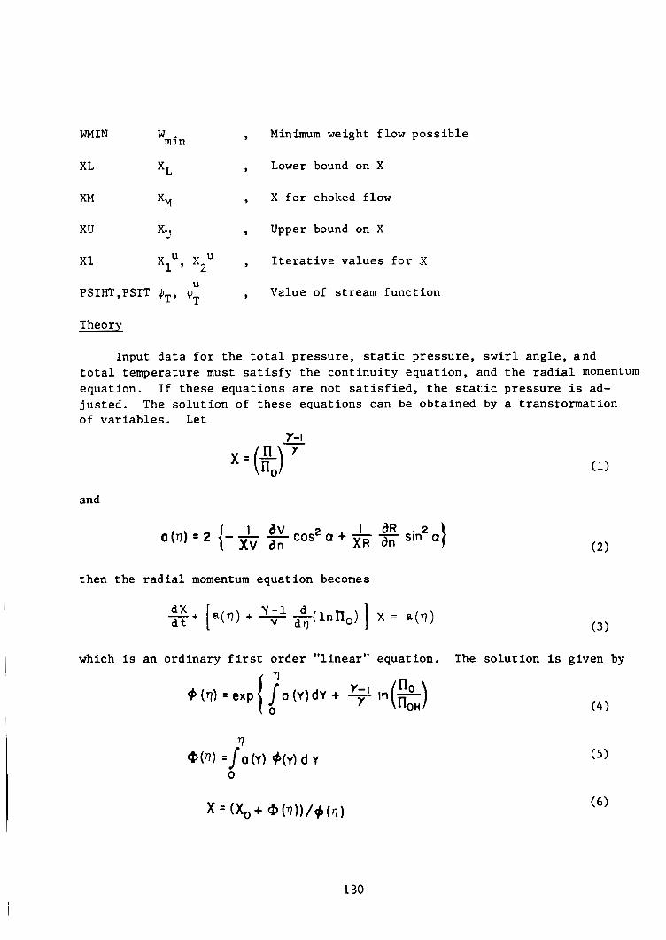
, Minimum weight f low p o s s i b l e 'm i n WIN
XL xL , Lower bound on X
XM xM , X f o r choked f low
xu , Upper bound on X
x1 XIU' x2u , I t e r a t i v e v a l u e s f o r X
PSIHT,PSIT +,, , Value of stream f u n c t i o n
Theorv
Input d a t a f o r t h e t o t a l p r e s s u r e , s t a t i c p r e s s u r e , s w i r l a n g l e , a n d
I f t h e s e e q u a t i o n s are not s a t i s f i e d , t h e s t a t i c p r e s s u r e is ad- t o t a l t empera ture must s a t i s f y t h e c o n t i n u i t y equa t ion , and t h e r a d i a l momentum equa t ion . j u s t e d . of v a r i a b l e s . L e t
The s o l u t i o n of t h e s e equa t ions can be ob ta ined by a t r ans fo rma t ion
Y-I x = (q)- n y
and
0(?77)=2 {-& %cos%+-- XR ' dn aR sin'.}
t hen t h e r a d i a l momentum equa t ion becomes
which i s an o r d i n a r y f i r s t o r d e r " l i n e a r " equa t ion . The : so lu t ion is g iven by r)
4 ('7) = exp 1 o (v) dv + - Y 0
130

I where x 0 i s t h e hub s t a t i c p r e s s u r e r a t i o . The c o n t i n u i t y equat ion becomes
The cons t an t Xo is determined by t h e boundary cond i t ion
W ( I ) = w
us ing an i t e r a t i o n scheme descr ibed below.
F i r s t l e t u s examine t h e f u n c t i o n
f(X) has a maximum a t I I
Hence from equa t ion (1)
Y
Equat ion (12) is p r e c i s e l y t h e c o n d i t i o n f o r choked flow when TI = 1. s t i t u t i o n of equa t ion (12) i n t o equat ion (10) y i e l d s an a p r i o r i cond i t ion f o r t h e maximum weight f low p o s s i b l e ( i .e . , t h e choked f low c o n d i t i o n ) . a subsonic s o l u t i o n w e t hen have t h e c o n d i t i o n
Sub-
For
2 < x < I Y + l
-
Furthermore, it i s noted t h a t w e can f i n d a p r i o r i Xo such t h a t
131

by s u b s t i t u t i n g equat ion (6) i n t o equat ion (10). bounds f o r choosing subsonic s o l u t i o n s wi th no reverse flow. The i t e r a t i o n scheme then c o n s i s t s of narrowing t h e bounds of XL and Xu u n t i l convergence occur s . This procedure is i l l u s t r a t e d i n f i g u r e 17 .
Thus XL and Xu are t h e
If ( P > \ I / ) x, V = xv . = \I/ I 2 v
and JI equa t ion ( 6 ) . Convergence occur s when
is obta ined by i n t e g r a t i n g equat ion ( 7 ) w i th Xo = X v+l s u b s t i t u t e d i n t o
Once X i s known, t h e s t a t i c p r e s s u r e i s ob ta ined from (1) and s u b s t i t u t e d f o r t h e inpu t s t a t i c p r e s s u r e .
132

Subrout ine C88R( J S ,KS)
Object Cont ro ls l o g i c i n determining coord ina te s and i n t e r p o l a t e s coord ina te s streamwise.
Options
IdPT9=O Computes approximate coord ina te s IdPT9iCO Coordinates s t o r e d on drum IdPT9=1 I!dPT9=3 Read coord ina te s from drum
Compute exac t coord ina te f u n c t i o n s and s t o r e on drum
L i s t of Symbols
DSTEP = AS , Streamwise s t e p s i z e (dimensionless)
DX = AX , I n t e r p o l a t i o n between J S and JS-1 s t a t i o n s
DXNEXT = AXN , I n t e r p o l a t i o n f o r nex t s t e p
JDRUM = , Drum u n i t number
JS = , J S t h s t a t i o n s t o r e d on drum
KS - - , KSth s t a t i o n i n t e r p o l a t e d between JS
- - zFl ZHUB
ZNEXT = ZN
, Axial s t a t i o n hub (d imens ionless )
, N e x t a x i a l s t a t i o n (dimensionless)
ZTIP = ZT , Axial s t a t i o n Tip (dimensionless)
Theory
L e t t h e streamwise c o o r d i n a t e S be g iven by
S = A S ( J S - I ) + dS* (KS- I )
where
A S = S, /(JUST - I )
(3) dS = AS/KDS
Then i f s t a t i o n 1 is a t JS-1 and s t a t i o n 2 a t JS , a s imple l i n e a r i n t e r p o l a t i o n of t h e c o o r d i n a t e s may be made from t h o s e s t o r e d on t h e drum. axial l o c a t i o n of t h e Ks+1 s t a t i o n .
ZNEXT i s t h e
133

Subroutine ( 3 8 ~ 5 (XH, XT, CURVH, CUF.VT)
Object
I Interpolate wall curvature at Station S
Options
None
Variables
XH
XT
CLJRVH
Arc length ID wall (dimensionless)
Arc length OD wall (dimensionless)
Curvature ID wall (dimensionless)
Curvature OD wall (dimensionless)
Table of XH (dimensionless)
Table of KH (dimensionless)
Table of % (dimensionless)
Table of 5 (dimensionless)
Theory
The values of %(S) and %(S) are input. Then the tables are searched and the values of s(S), KT(S) are calculated by linear interpolation.
134

Subrout ine C00RST
Ojbect Cont ro ls flow of coord ina te c a l c u l a t i o n
Options N~~~
L i s t of Symbols
DSTEP
DX
D Y 1
DY2
I C K
I1
ISLT1, ISLT2
1 \ 4 1 , I W 2
JC@JNT
KLHQLD
KN
MSLBT
NSL0T
UcI, J)
X
= AS = DS
= A n
= 6Y
= 62Y
= 0 , l
= 1 , 2
- -
P
= R ( I , ~ , J )
= x
Streamwise s t e p s i z e (dimensionless)
Normal coord ina te s t e p s i z e (dimensionless)
F i r st d e r i v a t i v e (dimens i o n l e s s )
Second d e r i v a t i v e (dimensionless)
Flag; no over lap , ove r l ap
F lag ; start i n t e g r a t i o n , cont inue i n t e g r a t i o n
F i r s t s l o t number, second s l o t number
F i r s t s l o t w a l l , second s l o t w a l l
Streamwise s t a t i o n coun te r
Number of s t r e a m l i n e s t o i n t e r p o l a t e
N u m b e r of streamlines t o i n t e g r a t e
S l o t counter
To ta l number of s l o t s
Temporary s t o r a g e f o r w a l l c o o r d i n a t e
, Normal coord ina te (dimensionless)
135

XM
x2
Y
Y1
Y2
Y3
z
ZZ1 ,ZZ2
Theory
= x
= x2
= Y
= Y(Xr)=Y1
= Y(X2)=Y2
= Y(X3)=Y3
= z
= zl, z2
, I n t e r p o l a t i o n d i s t a n c e (dimensionless)
, Midpoint of t h r e e p o i n t d i f f e r e n c e (d imens ionless )
, Funct ion t o b e in te rpola ted . (d imens ionless )
, Known v a l u e s of Y (dimensionless)
, Known v a l u e s of Y (d imens ionless )
, Known v a l u e s of Y (dimensionless)
, Axial d i s t a n c e (dimensionleas)
, Locat ion of a d j a c e n t s l o t s (d imens ionless )
T h i s s u b r o u t i n e c o n t r o l s t h e c a l c u l a t i o n flow f o r t h e c o o r d i n a t e s accord ing t o f low c h a r t f i g u r e 18. i s t o c a l c u l a t e t h e s t r e a m l i n e s through success ive ly l a r g e r d u c t s and s t o r i n g o n l y those c o o r d i n a t e s s a t i s f y i n g t h e c o n d i t i o n ( Z15ZLZ2) as shown in f i g u r e 1 9 .
The b a s i c c a l c u l a t i o n scheme wi th s l o t s
I n a d d i t i o n , i t w a s determined t h a t on ly KN s t r e a m l i n e s need b e c a l c u l a t e d by i n t e g r a t i o n , t h e remainder up t o KL s t r e a m l i n e s may b e c a l c u l a t e d u s i n g a p a r a b o l i c i n t e r p o l a t i o n .
136

Subrout ine C0bR1 (KSS,JSS)
Object Compute approximate coord ina te func t ions .
Theory
This sub rou t ine provides an i n i t i a l guess from t h e i terat ive method desc r ibed i n r e f e r e n c e 6 which is used t o approximate t h e coord ina te f u n c t i o n s and hence determine t h e numerical g r i d s t r u c t u r e used i n t h e f low a n a l y s i s .
Subrout ine ClwR3 (KSS , JSS ,L!BP)
Object Compute coord ina te f u n c t i o n s (10PT9=1,2).
Options
L&=1 Compute i n i t i a l c o n s t a n t s L0P=2 I n t e g r a t e one s t e p L@P=3 Do n o t i n t e g r a t e
L i s t of Symbols
A0 = A, , I n l e t h e i g h t W p lane (dimensionless)
ALO = ao , I n l e t a n g l e W p l ane (d imens ionless )
AN0 = n o , I n l e t he igh t Z p lane (dimensionless)
, I n i t i a l coo rd ina te l e n g t h (d imens ionless ) 0 SLO = SL
RO = ro , I n l e t r a d i u s Z p l ane (d imens ionless )
vo = . vo , I n l e t metric scale c o e f f i c i e n t (d imens ionless )
so = so , I n l e t streamwise coord ina te (d imens ionless )
XBO = 2, , Real p a r t of C1 (dimensionless)
YBO = ;o , Imaginary p a r t of C 1 (d imens ionless )
ZETA0 = 60 , Constant of i n t e g r a t i o n (real) (dimensionless)
ETA0 = ‘lo , Constant of i n t e g r a t i o n (imaginary) (d imens ionless )
Theorv
Using procedures desc r ibed i n r e f e r e n c e (6), one can i n t e g r a t e a long s t r e a m l i n e s t o g e t R, Z , V, S, N a t t h e l o c a t i o n of t h e p o l e s bI.
137

Subrout ine C88R4
Object Find Schwar tz -Chr is tof fe l parameters
Options
None
L i s t of Symbols
= % = xr
= aH
= s;
v = XT
= vy
= ho
= a,
= no
= sf
, Dis tance a long hub w a l l (d , imensionless)
, Dis tance a long t i p w a l l (d imens ionless )
, Wall a n g l e hub (deg)
, Wall a n g l e t i p (deg)
, Streamwise c o o r d i n a t e hub (dimensionless)
, Dis tance a long hub w a l l (d imens ionless )
, Metr ic scale c o e f f i c i e n t hub (d imens ionless )
, Radius hub (dimensionless)
, Streamwise c o o r d i n a t e t i p (dimensionless)
, Dis tance a long t i p w a l l (d imens ionless )
, Metric scale c o e f f i c i e n t t i p (d imens ionless )
, Radfus t i p (d imens ionless )
9 E r r o r i n SH (dimensionless)
9 Erro r i n sT (dimensionless)
, I n l e t he igh t W p l ane (dimensionless)
, I n l e t a n g l e W p lane (dimensionless)
, I n l e t h e i g h t Z p l a n e (dimensionless)
, I n i t i a l guess of c o o r d i n a t e l e n g t h (d imens ionless )
138

= r , I n l e t radius in Z plane (dimensionless) RO
vo = vo , I n l e t metric s c a l e coe f f i c i ent (dimensionless)
so = so , In le t streamwise coordinate (dimensionless)
XBO = xo , Real part of constant C 1 (dimensionless)
Y BO = Yo , Imaginary part of constant C1 (dimensionless)
ZETA0 = Eo , Constant of integration (real) (dimensionless)
0
2,
2,
ETA0 = o0 , Constant of integration (imaginary) (dimensionless)
The theory t o t h i s subroutine is described i n reference (1).
139
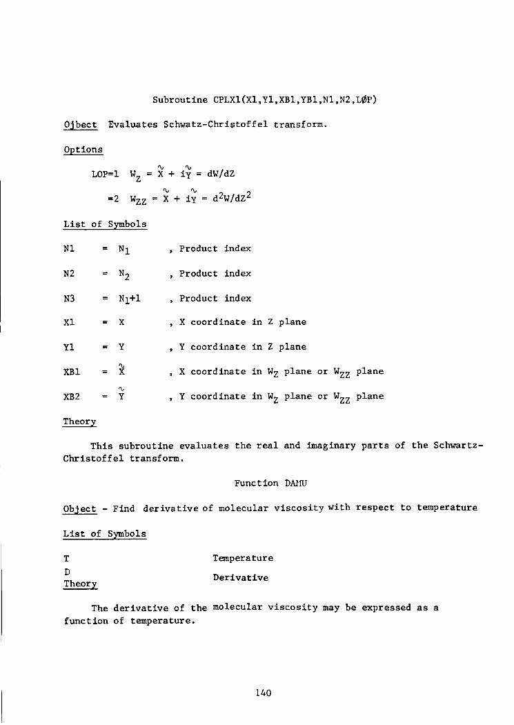
Subrout ine CPLX1(X1,Yl,XBl,YBl,Nl,N2,L@)
Ojbect Evalua tes Schwatz-Chr is tof fe l t ransform.
Options
‘L ’L LOP=1 Wz = X + i y = dW/dZ
L i s t of Symbols
N 1 = N 1 , Product index
N2 = N2 , Product index
N3 = N 1 + 1 , Product index
x1 = x , X c o o r d i n a t e i n 2 p lane
Y 1 = Y , Y c o o r d i n a t e i n Z p l ane
‘L xB1 = x , X coord ina te i n Wz p lane o r Wzz p l ane
XB2 = Y , Y c o o r d i n a t e i n Wz p l ane o r Wzz p l ane %
Theory
T h i s sub rou t ine e v a l u a t e s t h e real and imaginary p a r t s of t h e Schwartz- C h r i s t o f f e l t ransform.
Funct ion DMN
Object - Find d e r i v a t i v e of molecular v i s c o s i t y wi th r e s p e c t t o tempera ture
L i s t of Symbols
T Temperature D Theory
D e r i v a t i v e
The d e r i v a t i v e of t h e molecular v i s c o s i t y may be expressed as a f unc t ion of temperature .
140

D = A2 * (1.5/T - l/(T+ Al))
where
AI = 198./TX
A2 = T**1.5 * (l+Al) / (T+Al)
141

Object
Compute derivative of Roberts' transformation
Opt ions
LOP = 0 wall - wall boundary L0P = 1 wall-freestream boundary LBP = - 1 freestream-wall boundary
Input Variables
c = c 9 Distortion parameter
ETA = n 9 Input variable
LOP 9 Opt ion
Output Variable
DROBRT = a n / a r l , Output variable
Theory
The transform of the Roberts' Stretching for a d i s t 0 r t e . d mesh i s given by
where the options are
7'=? n = n } L $ P = O
We note that
i = 77/2 n = 2n'
7'= ( I + 7112 n = 2 n ' - 1 } L $ P = - I } L+P= I
0 s 31 I 1.0 o I n' s 1.0
142

Subrout ine DROUT (UNIT,ADDR,BLQCK)
Object Tape/Drum Read/Write d a t a
Opt ions - Entry P o i n t s
DR@UT(UNIT,ADDR,BL@CK)
Write on drum u n i t UNIT d a t a conta ined i n ADDR c o n t a i n i n g BL$CK number of words.
DRMIN(UNIT,ADDR,BL@CK)
Read from drum u n i t UNIT d a t a conta ined i n ADDR con ta in ing BLOCK number of words.
DREWND (UNIT)
Rewind drum u n i t UNIT.
DRMBKl (UNIT, ADDR , BMCIC)
Back space drum one BLOCK and r ead as i n DRMIN.
DRKBK2 (UNIT, ADDR, BLOCK)
Back space drum two BLOCK and r ead as i n DRMIN.
DPJIEOUF( UNIT)
Write end of f i l e on u n i t UNIT ( ' tape o n l y ) .
TPFILE (UNIT, LFILE)
Find f i l e number LFILE on t a p e u n i t UNIT.
Theory
Th i s sub rou t ine i s an 1/0 r o u t i n e to f a c i l i t a t e convers ion of UNIVAC NTRAN 1/0 r o u t i n e s t o o t h e r computer systems.
143

Subrout ine DRUTPE (LFILE, JBL@CK,L@PT)
Object T r a n s f e r s d a t a Drum/Tape o r TapelDrum.
Options
L6PT-1 L@PT=2
Trans fe r d a t a t a p e t o drum Trans fe r d a t a drum t o t a p e
L i s t of Symbols
JBL0CK - - , Number of r e c o r d s t o copy
JDRUM = , Drum u n i t number
I , Tape u n i t number JTAPE t
I , Tape f i l e number - LFILE -
Theory
T h i s sub rou t fne t r a n s f e r s d a t a us ing subrou t ine DRdUI'.
Subrout ine ERPTN(I1)
Objec t Checks normal p r e s s u r e g r a d i e n t f o r v i s c o u s f low
Opt ions
II=l Check i n l e t s t a t i o n I I = 2 Check J-1 s t a t i o n II=3 Check J s t a t i o n
L i s t of Symbols
ERP I N = c Theory
, E r r o r i n normal p r e s s u r e g r a d i e n t
A t any stat!.on i n t h e d u c t , t h e normal momentum equa t ion must b e s a t i s f i e d . Th i s sub rou t ine cRecks t h e e r r o r .
144 I

v/c,
M
Function FAMACH (AN)
Object
Variables
AN
FAMACH
Theory
Calculate Mach number from velocity
The Mach number can be calculated from
Velocity/stagnation speed of sound
Mach number
r-1 2 112 = M/(1 + -j- PI
cO
using Newton's method.
145

Subrout ine FAVER2
Object Solve f o r mass f low weighted average flow and output parameters .
Options
N me
L i s t of Symbols
AAR
AMA
AMACHE
AMFH
AMFT
AMG
AMM
ASH
AST
ATFH
ATFT
CFH $
CFT 4
Q
CPC
CPCgm
CPJNC
DASHl,DASH2
, Area r a t i o ( d h e n s i o n l e s s )
, L o c a l Mach number (dimensionless)
, Area average Mach number (dimensionless)
, Wall b leed hub (dimensionless)
, W a l l b leed t i p (dimensionless)
, Midpoint Mach number (dimensionless)
, Maximum Mach number (d imens ionless )
, Sur face area hub w a l l (d imens ionless )
, Surface area t i p w a l l (dimensionless)
, Heat f l u x / l e n g t h hub (d imens ionless )
, Heat f l u x / l e n g t h t i p (d imens ionless )
, Wall f r i c t i o n c o e f f i c i e n t hub (dimensionless)
, Wall f r i c t i o n c o e f f i c i e n t t i p (dimensionless)
= 1,2,3 f o r J+1-4 s t a t i o n
= P r / q l , Normalizing f a c t o r f o r Cp d imens ionless
, P r e s s u r e c o e f f i c i e n t (compress ib le ) (d imens ionless )
, Pressu re c o e f f i c i e n t ( incompress ib le ) (d imens ionless )
, Area increment hub (d imens ionless )
= CPC
= cPI
= %H
146
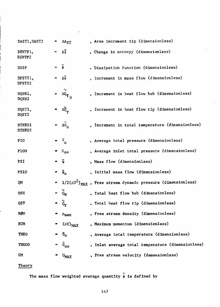
DASTl,DAST2
DENTP 1, DENTP2
DISP
DPSTI1, DPSTI2
DQSHl, DQSH2
DQST1, DQST2
DTHEO 1 DTHEO 2
PI0
PI00
PSI
PSI0
QN
QSH
QST
R0M
RUM
THE0
THE00
UM
1
Theory
= U S T , Area increment t i p (d imens ionless )
= A T , Change i n en t ropy (d imens ionless )
- = @ , D i s s i p a t i o n f u n c t i o n (d imens ionless )
= A 5 , Increment i n mass f low (d imens ionless )
, Increment i n h e a t f low hub (d imens ionless )
= A a T , Increment i n hea t f low t i p (d imens ionless )
- = AOo , Increment i n t o t a l t empera ture (d imens ionless )
, Average t o t a l p r e s s u r e (d imens ionless )
, Average i n l e t t o t a l p r e s s u r e (d imens ionless )
0 n
= 00
5 , Mass f low (dimensionless)
$0 , I n i t i a l mass f low (d imens ionless )
1 / 2 ( p U 2 ) ~ , F r e e stream dynamic p r e s s u r e (dimensionless)
QH
-
% , T o t a l h e a t f low hub (dimensionless)
, T o t a l h e a t flow t i p (dimensionless)
, F r e e stream d e n s i t y (dimensionless)
, Maximum momentum (dimensionless)
, Average t o t a l t empera ture (d imens ionless )
, I n l e t average t o t a l t empera ture (dimensionless)
, Free stream v e l o c i t y (demensionless)
%
QT
Pmax
(PU) MAX
60
000
%Ax
-
The mass f low weighted average q u a n t i t y I$ i s de f ined by
147
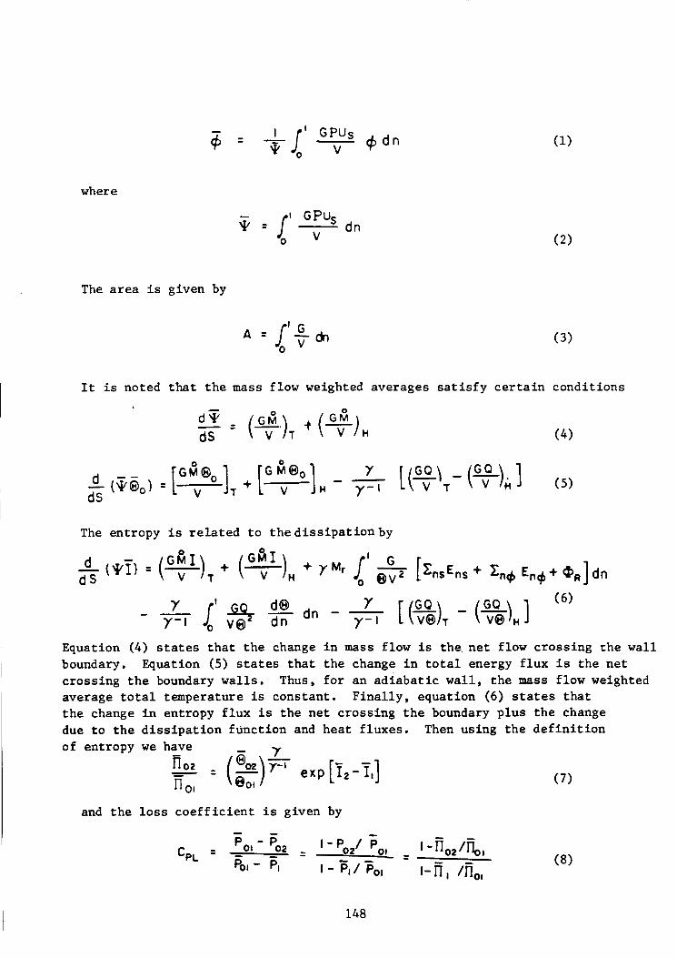
where
d n - - J1 GPUs V q - 0
The area i s g iven by
A = a'%* (3 )
It is noted that t h e m a s s f low weighted ave rages s a t i s f y c e r t a i n c o n d i t i o n s
The en t ropy is r e l a t e d t o t h e d i s s i p a t i o n b y
Equat ion ( 4 ) states t h a t t h e change i n mass f low is t h e n e t f low c r o s s i n g t h e w a l l boundary. Equation (5) states t h a t t h e change i n t o t a l energy f l u x i s t h e n e t c ros s ing t h e boundary walls. Thus, f o r an a d i a b a t i c w a l l , t h e mass f low weighted average t o t a l t empera ture is cons t an t . F i n a l l y , equat ion (6) states t h a t t h e change i n en t ropy f l u x i s t h e n e t c r o s s i n g t h e boundary p l u s t h e change due t o t h e d i s s i p a t i o n f u n c t i o n and h e a t f l u x e s . Then us ing t h e d e f i n i t i o n
I
- Y of en t ropy w e have
(7)
and t h e l o s s c o e f f i c i e n t i s g iven by
I 148

I f w e now de f ined t h e mass f low weighted ave rages I
This sub rou t ine a l s o c a l c u l a t e s Some q u a n t i t i e s p r i n t e d i n t h e summary a t t h e end of t h e v i scous c a l c u l a t i o n .
The p r e s s u r e c o e f f i c i e n t i s de f ined by :
I ?,
An e f f e c t i v e area A can b e de f ined as t h e geometr ica l area minus t h e block- a g e caused by t h e boundary l a y e r . of maximum v e l o c i t y a c r o s s t h e duc t w e have by d e f i n i t i o n
I f w e d e f i n e t h e f r ees t r eam as t h e po in t :
Hence, t h e blockage B i s de f ined as
8 = I - A/A,tt = I-m/(p-U,A)
The area averaged ( e f f e c t i v e Mach number) may then be de f ined by t h e i s e n t r o p i c f l o w r e l a t i o n s . Thus,
The e f f e c t i v e n e s s TI of t h e d i f f u s e r i s based on an i d e a l i s e n t r o p i c f low w i t h t h e m a s s f low weighted average Mach numbers. c o e f f i c i e n t is g iven by
Thus, t h e i d e a l p r e s s u r e
149

i7 - n l = n,,n,
where
Then
- 7) = CP'CPI
The wall f r i c t i o n coe f f i c i ent i s defined a s
C f = z w / ( $ P u 2 ) MAX
The wall surface area and heat flow are determined by integrating the equations
using the trapezoid ru le .
150

1 , Funct ion FCgLES (Argument L i s t )
, Object Compute Coles v e l o c i t y p r o f i l e f o r boundary l a y e r a t i n i t i a l s t a t i o n .
Options
None
L i s t of Symbols
AK = K , Von Karman c o n s t a n t
APLS = A+ , Van Driest c o n s t a n t
AP I = M , Coles shape f a c t o r
AKPL = KS , Roughness Reynolds number
DELT = , Boundary l a y e r t h i c h e s s
DAMP = D , Damping f a c t o r
P I = 71 , 3.14159
Y = Y , Dis tance from w a l l
YPLUS 5 y+ , Unive r sa l d i s t a n c e
UPLU s = u+ , Unive r sa l v e l o c i t y
FCQILES = uc , Coles v e l o c i t y (output)
Theory
+
+
This s u b r o u t i n e i n t e g r a t e s t h e d i f f e r e n t i a l equa t ion f o r t h e i n n e r l a y e r g iven by
w i t h t h e damping f a c t o r , r e f e r e n c e s (7, 81, given by
D =1-exp (-5) + ( I + * 30 Y +)t?XP(-23$)
151

and adds Coles' wake function (reference 3 ) , given by
152

Subrout ine FCORCT
Object Correc t t r u n c a t i o n e r r o r
Options None
L i s t of Symbols
AMUW = pw/M , Wall v a l u e of v i s c o s i t y (d imens ionless )
DU - - AU , Veloc i ty d i f f e r e n c e (d imens ionless )
EC#R = (pU)/(pU), Mass f l u x r a t i o (d imens ionless
EMB - - , Erro r i n Mach number (dimensionless)
EPB - - E E r r o r i n s t a t i c p r e s s u r e (d imens ionless )
ERB - - , Erro r i n d e n s i t y (dimensionless)
E m
P
E R
, Erro r i n s t a t i c tempera ture (d imens ionless ) ET - ETB -
Erro r i n v e l o c i t y (d imens ionless ) U E - EUB -
, Erro r i n s w i r l v e l o c i t y (d imens ionless ) UP
E - EUP -
EU S - - , E r r o r i n streamwise v e l o c i t y (dimensionless)
, S t r a i n - E!,
EW -
Theory
The point- to-point i n s t a b i l i t y desc r ibed i n r e f e r e n c e 6 i s minimized by r e c a l c u l a t i n g t h e stresses and h e a t f l u x us ing c e n t r a l d i f f e r e n c e s r a t h e r t h a n cen te red d i f f e r e n c e s .
153

Subrout ine FCPLX
Object Evaluates complex f u n c t i o n s f o r e x a c t coord ina te c a l c u l a t i o n .
Opt i ons
L0PT = 1 LdpT = 2 Compute only d e r i v a t i v e s
Compute and s t o r e f u n c t i o n s and d e r i v a t i v e s
L i s t of Symbols (Note s u b s c r i p t n o t a t i o n f o r d e r i v a t i v e s used)
I N l , N 2
xs
XN
x sx
XSY
XD
XZETS
XETAS
XXS
XYS
X B 1
YB1
x1
Y 1
XDB
XNZET
XNETA
xv
N1"2
S
n
Sx = n
= n
Y
sY x
5, = rln
os = -5
D
n -
xs - Yn
Ys = x n % - x = 5, - ny
Y = -Ey = rlx %
X
Y
D -
"5
n
v rl
154

xsxx 1
x SXY
xxss
XXSN
X B 2
Y B 2
xzss
XZ SN
XDBN
XDBS
XESDN
XESDN
XZ SDN
XZSDS
XVN
XVS
X E S S
XESN
X D I S
XDIN
- sxx - s =
XY
n xx
n YY
S YY
n xx
'ss = Yns = xnn
x = 5,, = Qyx - - -Cxy
= Y = -Exy = -Qyy - -nxx
"n
Qss
'lsn
Dn
155

Theory
The theo ry f o r e v a l u a t i n g t h e complex f u n c t i o n s and a l l d e r i v a t i v e s is de r ived i n r e f e r e n c e ( 6 ) . With t h e u s e of o r t h o g o n a l i t y r e l a t i o n s which are i m p l i c i t i n t h e theory of complex f u n c t i o n , t h e f u n c t i o n s and d e r i v a t i v e s may be eva lua ted . It i s noted t h a t t h i s sub rou t ine w a s programmed t o accep t m u l t i p l e sou rces i n t h e z p lane , a l though only one i s used i n t h e p r e s e n t c a l c u l a t i o n . The de r ived f u n c t i o n s c a l c u l a t e d i n t h i s sub rou t ine are l i s t e d as fo l lows:
NS
1-1 n = 1 AI tan" [ y / ( X - bI)]
X, = - S,/D
156

7)s = TX xs+ 3yys
I v =
-353 I sxxxs+ D sxyys D2 x s s = -
Numerical accuracy can be s ign i f i cant ly improved by ordering the way i n which sums and products are made. A s an example, the f i r s t equation, equation (11, may be written
157

Thus t h e squa re r o o t of t h e sum of squa res of 0(1) and S = 0 ( IX-bII). r u l e h a s been a p p l i e d t o a l l equa t ions by e x t r a c t i n g t h e o r d e r of magnitude of t h e term from each c a l c u l a t i o n .
Th i s
Subrout ine FETA (B, ETA, AN, DEDN, D2EDN)
Object
C a l c u l a t e d i s t o r t e d mesh t o be used i n Subrout ine P b I S
Options
B = O Uniform mesh (no s t r e t c h i n g ) B > O Tanh s t r e t c h i n g
V a r i a b l e s
B
ETA
AN
DEDN
DZEDN
, Constant
n , Transformed Normal Coordina te
n , Normal Coordinate
a n / an
a%/ an2
Theory
Th i s s u b r o u t i n e c a l c u l a t e s t h e d i s t o r t e d mesh t h a t w i l l be used i n c a l c u l a t i o n by s u b r o u t i n e PQIS. The t r ans fo rma t ion i s g iven by
q = t anh [Bn]/tanh [ B ] B ’ n = n B = O
158
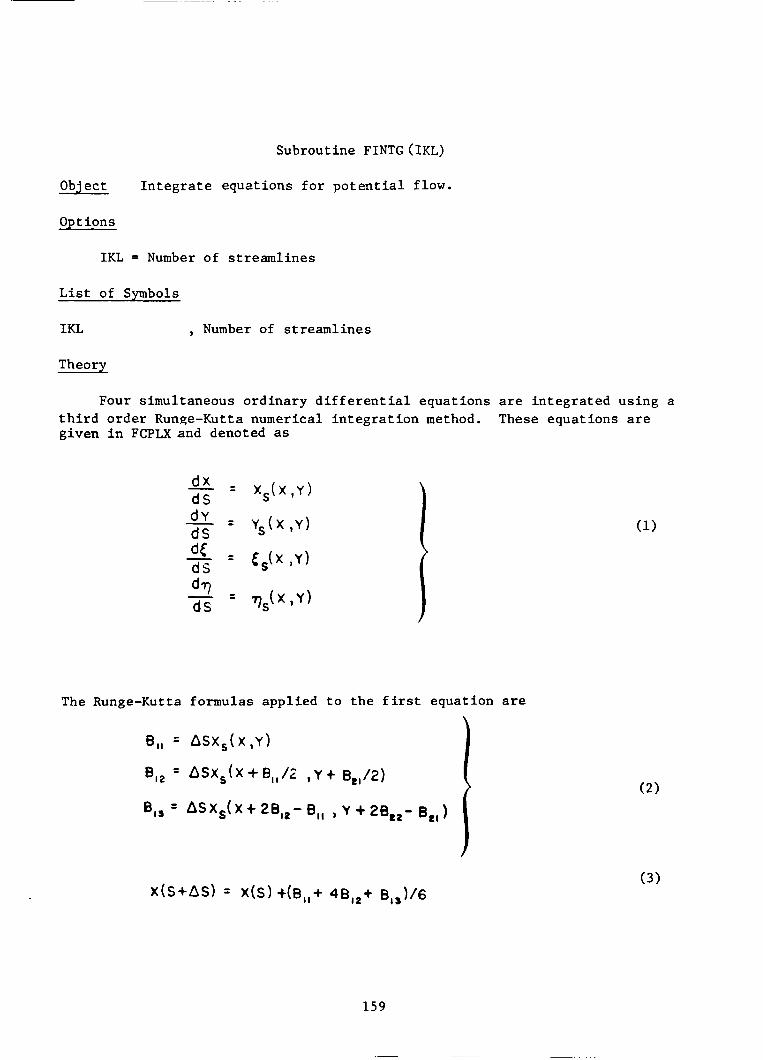
Subrout ine FINTG (IXL)
Object I n t e g r a t e equa t ions f o r p o t e n t i a l flow.
Opt i o n s
IKL = Number of s t r e a m l i n e s
L i s t of Symbols
IKL , Number of s t r e a m l i n e s
Theory
Four s imul taneous o r d i n a r y d i f f e r e n t i a l equa t ions are i n t e g r a t e d u s i n g a t h i r d o r d e r Runge-Kutta numer ica l i n t e g r a t i o n method. g iven i n FCPLXand denoted as
These equa t ions are
- = d x Xs( X , Y )
- d y = Y S ( X , Y )
- - dc - &(x , Y )
d S
dS
dS
dS - -
The Runge-Kutta formulas a p p l i e d to t h e f i r s t equa t ion are
B,, = A S X , ( X , Y )
B,, = A S X , ( X + B , , / 2 , Y t B,,/2)
Bls = A S X s ( X t 2B,,- B,, , Y + 28,,- Bel)

Subrout ine FL0WIN
Object Setup i n l e t f low.
I Opt ions
I0PT1 = 1 Compute i n l e t f low If (To=O) Po=P 1: and To=Tr
If ( ~ , > 1 0 . ) Normalize wi th Tr and Pr I0PTl = 2 Read i n l e t f low
L i s t of Symbols
BINP (I , J , K ) , I n t e r p o l a t e d from BINPUT(IH,J,L)
Theory I@PT1=1
For t h i s o p t i o n t h e f r ees t r eam f low is assumed t o b e i s e n t r o p i c wi th a c o n s t a n t f r e e s t r e a m Nach number Ifs and w a l l boundary l a y e r s de f ined by power- l a w v e l o c i t y p r o f i l e s . t h e normal momentum equa t ions must be s a t i s f i e d t o g e t h e r w i th i s e n t r o p i c r e l a t i o n s h i p s of p r e s s u r e r a t i o and tempera ture r a t i o .
S ince t h e s w i r l i n g f low must be i n r a d i a l equ i l ib r ium,
Neglec t ing c u r v a t u r e i n t h e mer id iona l p l ane
where
Y- I
1 Equation (1) can be i n t e g r a t e d wi th
and
160

as i n i t i a l c o n d i t i o n s us ing a Runge-Kutta method.
For a g iven displacement t h i c k n e s s and v e l o c
and
t y prof l e power l a w , w a l l boundary l a y e r s can be added, assuming c o l l a t e r a l boundary l a y e r s , such t h a t a i s unchanged. Then
A= ( i + n ) A *
F i n a l l y , t h e i n l e t m a s s f low and r e f e r e n c e v e l o c i t y are determined as follows
Theory I@PT1=2
For t h i s op t ion , t h e inpu t f low i s c a l c u l a t e d from exper imenta l i npu t d a t a . The inpu t v a r i a b l e s s e l e c t e d are spanwise l o c a t i o n , t o t a l p r e s s u r e , s t a t i c p r e s s u r e , f low ang le , and t o t a l t empera ture , s i n c e t h e s e are t h e p r i - mary measured v a r i a b l e s . A s imple l i n e a r i n t e r p o l a t i o n is used so t h a t f o r any v a r i a b l e @,
161

The f low v a r i a b l e s are c a l c u l a t e d from equa t ions 1 through 7.
I f (T- > lo), i t is assumed t h a t p r e s s u r e and temperature are g iven i n ( p s f ) and deg R , r e s p e c t i v e l y , and t h e f low i s normalized accord ingly . is g iven , it is assumed t h a t boundary l a y e r s should be added accord ingly t o t h e v e l o c i t y p r o f i l e power l a w above. v e l o c i t y are determined from equa t ions 9 and 10. A flow c h a r t of t h i s sub- r o u t i n e is p resen ted i n f i g u r e 20.
I f 6*
F i n a l l y , t h e weight f low and r e f e r e n c e
162

Subrout ine FN0RM
I Object Normalize inpu t y a r i a b l e s . Opt ions
I
I
None
L i s t of Symbols
All v a r i a b l e s i n C@MM@N blocks
Theory
All i npu t v a r i a b l e s are normalized accord ing t o t h e L i s t of Symbols.
163

Subrout ine F@RCE/PRQIP
Object Compute b l a d e f o r c e s
Opt i o n s
N ~ P P F = 1
NbPPF = 0
Rad ia l , a x i a l , and s w i r l b lade f o r c e s are def ined i n p r o p e l l e r p o r t i o n of program.
Rad ia l , a x i a l , and s w i r l b l ade f o r c e s are read from inpu t .
L i s t of Symbols
FRCI(N, 1) Blade f o r c e ( r a d i a l d i r e c t i o n ) / s p a n
FRCI(N, 2) Blade f o r c e ( p h i d i r e c t i o n ) /span (d imens ionless )
FRCI(N, 3) Blade f o r c e ( a x i a l d i r e c t i o n ) / s p a n (nondimension)
FRC(N, 1) Blade f o r c e ( r a d i a l d i r e c t i o n ) / s p a n (nondimension)
FRC(N, 2) Blade f o r c e ( p h i d i r e c t i o n ) /span (nondimension)
FRC(N, 3) Blade f o r c e ( a x i a l d i r e c t i o n ) / s p a n (nondimensional)
FflRC(3, K) Blade f o r c e ( s t ream di rec t ion) /volume (nondimensional:
FgRC(4, K) Blade f o r c e ( swir l ) /vo lume (nondimensional)
c o s i n e of 8 FLaC(5, N)
K Index of rl coo rd ina te
N Index of p o i n t s a long p r o p e l l e r c e n t e r l i n e
Theory
Th i s sub rou t ine i s used t o c a l c u l a t e t h e streamwise and s w i r l b l a d e com- ponents f o r each s t r e a m l i n e . I t i s assumed t h a t t h e normal component is small. The p rocess has two s t e p s . (1st) Ca lcu la t ion of r a d i a l , a x i a l , and p h i b l a d e f o r c e components f o r each
s t r e a m l i n e by us ing l i n e a r i n t e r p o l a t i o n of b l ade p o i n t s .
(2nd) Convert ing r a d i a l , ax ia l , p h i b l ade f o r c e components t o streamwise and s w i r l b l ade f o r c e s .
164

Subroutine F0RCL
Object Compute loca l blade force.
Options None
L i s t of Symbols
GAP = G , Strut gap (dimensionless)
ZLE
ZTE
Theory
, Location of leading edge (dimensionless) = 'LE
- 'TE - , Location of t ra i l ing edge (dimensionless)
The chordwise distribution of blade loading (force/voluma) i s defined by
In t h i s subroutine, the chordwise loading i s assumed uniform.
165
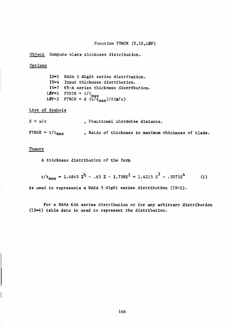
Object Compute blade thickness distribution.
Opt ions
IS=1 NASA 5 digit series distribQtion. IS14 Input thickness distribution. IS=7 65-A series thickness distrfbution.
L6P=1 FTHIK = t/tm L0P=2 FTHIK = d (t$tmax)/d(x/c)
List of Symbols
z = x/c , Fractional chordwise distance.
FTHIK = t/t,, , Ratio of thickness to maximum thickness of blade.
Theory
A thickness distribution of the form
t/t,, = 1.4845 i' - .63 2 - 1.758Z2 + 1.4215 Z3 - .5075Z4 (1 1
is used to representa a NASA 5 digit series distribution (IS=l).
For a NASA 65A series distribution or for any arbitrary distribution (IS=4) table data is used to represent the distribution.
166

Subrout ine GBLADE
Object Compute Blade Geometry
Options None
L i s t of Symbols
ALPHS a
CHRD B
r
, Stagger a n g l e t o a x i s (deg)
, (Local) b l ade chord (d imens ionless )
GAP G I R T ISHAF'E
, Gap between b l ades (d imens ionless )
, Blade shape (Option) Index Counter
NBLADE , Number of b l ades i n one row
N R W , Number of b l ade rows
NUM , Number of p o i n t s a long b l ade c e n t e r l i n e
PHIC , Blade camber
RCLH RCLH , Hub r a d i u s of b l ade c e n t e r l i n e
RCLT R~~~ ,
, S o l i d i t y
Tip r a d i u s of b l ade c e n t e r l i n e
SLD a
THICK , Local b l a d e t h i c k n e s s t
THICKN , Blade t h i c k n e s s
t / B , Maximum th ickness /chord THIKM
- Z ZBAR , Axial p o s i t i o n w i t h r e s p e c t t o b l ade
z CL ZCL , Blade a x i a l c e n t e r l i n e
ZCLX zcLx , Axial d i s t a n c e t o b l ade c e n t e r l i n e
ZKK , F r a c t i o n a l d i s t a n c e a long c h o r d l i n e
ZLE 'LE , Blade l ead ing edge
167

ZTE
CONST(1, L)
CONST(2, L)
CONST(3, L)
CONST(4, L)
CONST(5, L)
Blade t r a i l i n g edge
Radius ( inpu t d a t a )
Stagger ang le ( i n p u t d a t a )
Chord ( inpu t d a t a )
Thickness t o chord r a t i o ( inpu t d a t a )
Camber ang le ( inpu t d a t a )
Axial d i s t a n c e ( inpu t d a t a )
Radius
Gap
Normal d e r i v a t i v e of b l ade s u r f a c e
Streamwise d e r i v a t i v e of b l ade s u r f a c e
Th i s module i n t e r p o l a t e s b l ade d a t a w i t h r e s p e c t t o t h e r a d i u s of b l a d e s i n o r d e r t o o b t a i n l o c a l b l a d e informat ion . The fo l lowing parameters are i n t e r p o l a t e d ; a, B, t / B , $c, and ZcLy. l a t e d i n FTHIK and used t o determine G , aG/an and a G / a s . A f low c h a r t is given i n F ig . 21.
The b l ade t h i c k n e s s is t h e n ca lcu-
168

Subrout ine GDUCT
Object Compute Duct shape
Options
IQ)PT3=1 S t r a i g h t annu la r duc t XQ)PT3-2 Read duc t shape I0PT3=3 S t r a igh t -wa l l d i f f u s e r IOPT3=4 NACA curved-wall d i f f u s e r
L i s t of Symbols
( A s needed by u s e r )
Theory
Th i s s u b r o u t i n e is used t o p r e s c r i b e t h e duc t shape r H ( Z ) , r T ( Z ) , w a l l b leed iH(Z), gT(Z) , and w a l l t empera ture TH(Z), TT(Z), as r equ i r ed . S ince t h e s e f u n c t i o n s are i n p u t , t h e programmer may write a s u b r o u t i n e f o r t h i s purpose o r r ead t h e r equ i r ed informat ion accord ing t o I0PT3. I n a d d i t i o n , t h e sub rou t ine computes t h e r e f e r e n c e r a d i u s and normal izes t h e v a r i a b l e s r and T. The v a r i a b l e m is normalized i n Subrout ine FL0WIN when U r is c a l c u l a t e d .
0
Input /Output
The u s e r may program any duct shape and w a l l boundary c o n d i t i o n s as The ou tpu t of t h i s sub rou t ine must be ( R ( I , K , J ) , I=1,3; K=1,2, r equ i r ed .
J = l , J L ) and 21. Note t h a t a l l v a r i a b l e s are normalized as shown i n t h e sample subprogram desc r ibed i n t h e Subrout ine GDUCT l i s t i n g and t h a t e q u a l l y spaced spanwise s t a t i o n s are used. The f lowchar t ( f i g u r e 22) should be fol lowed i n programming.
169

Subrout ine GE~JMCL
Object C a l c u l a t e c o o r d i n a t e s of l i f t i n g l i n e .
Options
None
L i s t of Symbols
- - AL
AM 3
AN1, AN2 =
ANI, ANI1 =
3 ANL
B1, R2
R I , R I 1 =
RL
t
- -
s1, s2 =
SI , S I 1 =
= SSL
21, 22 =
Z I , Z I 1 =
CONS(1,L) =
CONS(2,L) =
CONS(3,L) =
CONS(4,L) =
CONS(6,L) =
*L
AM
N 1 , N2
N I , N I - 1
NL
R1’ R2
RI, RI-l
RL
s2
sI-l
sL
z 1 9 z2
Z I 9 Z I - 1
RL
a L
BL
( t / B ) L
ZCL
, Slope of l i f t i n g l i n e
, Slope of coord ina te l i n e
, N coord ina te of g r i d
, N coord ina te of l i f t i n g l i n e i n t e r s e c t i o n w i t h g r i d
, N coord ina te of i npu t p o i n t of l i f t i n g l i n e
, R coord ina te of g r i d l i n e
, R coord ina te of l i f t i n g l i n e i n t e r s e c t i o n w i t h g r i d
, R c o o r d i n a t e of l i f t i n g l i n e inpu t
, S coord ina te of g r i d
, S coord ina te of l i f t i n g l i n e i n t e r s e c t i o n wi th g r i d
, S coord ina te of l i f t i n g l i n e inpu t p o i n t
, 2 coord ina te of g r i d l i n e
, Z coord ina te of l i f t i n g l i n e I n t e r s e c t i o n w i t h g r i d
, L i f t i n g l i n e r a d i u s (Local)
, Stagger a n g l e (Local)
, Chord (Local)
, Thickness/chord ( l o c a l )
, L i f t i n g Line Axial Di s t ance ( l o c a l )
170

CONS(8,L) nL
C O N S ( ~ , L ) sL
L i f t i n g l i n e normal l o c a t i o n s
L i f t i n g l i n e streamwise l o c a t i o n
Theory
The equat ion f o r t h e l i f t i n g l i n e pass ing through t h e p o i n t s (L, L-1) i s approximated by a l i n e given by
The s t r e a m l i n e coord ina te system forms a box around t h e L-1 mesh p o i n t ( s e e f i g u r e 23) given by t h e p o i n t s (11, (21 , (31, (4). I f it i s assumed t h a t p o i n t ( 5 ) i s known; t h e o b j e c t i s t o f i n d p o i n t (6) by success ive ly checking each s i d e of t h e mesh t o determine i f t h e l i f t i n g l i n e c r o s s e s . L e t t h e index I = 1, 4 r e p r e s e n t each s i d e of t h e box. l i n e i s passed through t h e p a i r of p o i n t s
Then a s t r a i g h t
I Points
2 (31 , (2) S2 - n v a r i e s
3 (41, (3) n2 - S v a r i e s
4 (11, (4) S, - n v a r i e s
The equat ion of t h e s t r a i g h t l i n e approximating t h e l i f t i n g l i n e is g iven by
171
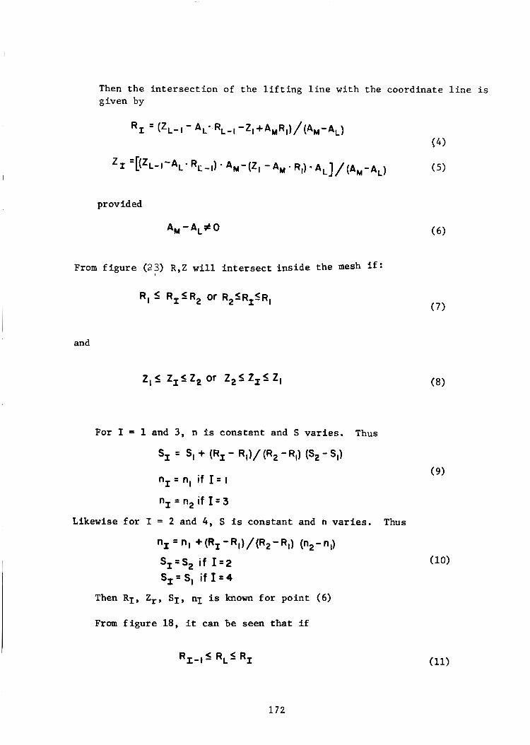
Then t h e i n t e r s e c t i o n of t he l i f t i n g l i n e wi th t h e coord ina te l i n e is g iven by
pr ov i d ed
A u - A L f O
From f i g u r e (23) R , Z w i l l i n t e r s e c t inside t h e mesh if:
R, 5 R, IR2 or R~IR,IR,
and
2, I Z, IZ , or Z 2 1 2,s Z,
For I = 1 and 3, n 2s c o n s t a n t and S v a r i e s . Thus
s, = s, + (Rr: - RI)/ (R2 -R,) F, - SI) nI= nI if I = I
nI = n2 if I = 3
Likewise f o r I = 2 and 4, S i s c o n s t a n t and n v a r i e s . Thus
"1 = " I +(R*-R, ) /P2-R1) (n2-q)
S,=S, if I=2 S,=S, if I=4
Then RI, Zr , SI, nI is known f o r p o i n t (6)
From f i g u r e 18 , it can be seen t h a t i f
( 7 )
R,,,I R,S R,
172

RL l i e s within the grid (l), ( 2 ) , ( 3 ) , ( 4 ) , and L should be advanced. n and S vary along the l i f t i n g l i n e . then nL, SL can be determined by the re lat ions
Both I f (RL, ZL) l ies within the grid
s,= S I + ( s ~ - S I - l V ( R f R1-1) (RL- RL-1)
"L = '1-1 + (nI-nI-i)/ (12) - ~ 1 - 1 1 ( R ~ - R ~ - ~ )
This procedure can then be repeated for L = 2 , NUM
173

Subroutine INITQ
JS TEP
R
Z
aR/ an
, Block (record number)
, Radius (dimensionless)
, Axial distance (dimensionless)
, Derivative
aR/as , Derivative
, Axisymmetric flow angle 2 axi (case)
V , Metric coefficient (dimensionless)
avian= ( K + L K ~ ) , Curvature of streamline S
av/ as , Curvature of potential line
X
Y
Y/YT
A
G
aG/ an
aG/ as
, Distance along streamline (dimensionless)
, Duct height (dimensionless)
, Normalized duct height
, Duct Area (dimensionless)
Gap (dimensionless)
, derivative
, Derivative
anIan , Transformation of normal coordinate
174

Subroutine INITQ (Cont'd)
n
rl
K = 1, KL
r r
JL
KL
, Not used
, Normal coordinate (dimensionless)
, Transformed coordinate
, Reference radius, (ft)
, Not used
, Number of streamwise steps
, Number of streamlines
This subroutine initializes the indepenLmt varia le array BLOCK which is stored on a disc file and sets all parameters QPARM required by the calculation.
Note that Q ( 7 , K ) stores either Ks or Ks+AKs. *
175

Subroutine INTFRE
Object
Initialize freestream conditions
Opt ions
None
List of Symbols
See C8MF18N BL8CKS
Theory
Data read from f i l e NDRUM is used to setup the freestream conditions for subroutine P0IS.
176
Obj ect Loader f ormated inpu t
Opt i o n s
N@PT8=O Continue r ead ing N@PT8=1 Stop r ead ing inpi
Subrout ine L@ADRR
i n p u t t
L i s t of Symbols
See EQUIVALENCE ARRAYS i n s u b r o u t i n e l i s t i n g s .
Theory
Th i s method of r ead ing inpu t pe rmi t s t h e changing of one o r more inpu t v a r i a b l e s . case.
The remaining inpu t v a r i a b l e s remain t h e same as t h e p rev ious
177

Subrout ine MINVRT(A,B,N)
Object I n v e r t NxN mat r ix .
Options
None
L i s t of Symbols - -
A = E , Augmented ma t r ix
B = B , Augmented m t r i c (A-1) mat r ix - -
N , Number of equat ions (rows)
M , Number of columns
Theory
The x mat r ix i s inve r t ed us ing t h e Gauss-Jordan e l i m i n a t i o n procedure. F i r s t t h e augmented $ ( N , M ) i s formed inc lud ing t h e i d e n t i t y m a t r i x ,
Then t h e fo l lowing r e v i s i o n formula i s used
= a /a N , J - I IIJ Ill
b 1 < J S M (3)
Note t h a t t h e 5 matrix has one less column than t h e 5 matrix. s u b s t i t u t i o n is made
Then t h e
' I J = b I J
and repea ted u n t i l t h e ma t r ix is an NxN o r t h e w' matr ix .
178

' Subrout ine MYTIME
Object Dummy t i m e t r a p r o u t i n e
Subrout ine 0UTPUT I 1 I
Object
P r i n t t i t l e page
Option
None
L i s t of Symbols
None
Theory
T h i s s u b r o u t i n e p r i n t s t h e t i t l e page which r e c o r d s a l l m o d i f i c a t i o n s , d a t e s , and r e f e r e n c e s t o changes incorpora ted i n t o t h e ADD code.
179

Subrout ine PERFNA
Object Compute v i s c o u s n a c e l l e drag
Opt i o n s
None
L i s t of Symbols
AREAM
CDFR
- - I Amax
= C~~
CDPR = ‘DP
I DFR = DF
QREF = Qr
RMAX
AVE(9,l) = P1
AVE(4,l) = U1
P = P
- - Rmax
P1 ,P2 = n p n 2
R = R
R 1 ,R2 = R 1 , R 2
S = S
s1 s2 = s1,s2
Theory
I n terms of d imens ionless v a r i a b l e s used i n t h e a n a l y s i s , t h e f r i c t i o n and p r e s s u r e drag are g iven by:
Maximum c r o s s - s e c t i o n a l area
F r i c t i o n drag c o e f f i c i e n t
P res su re drag c o e f f i c i e n t
F r i c t i o n drag ( l b )
Reference dynamic p r e s s u r e ( p s f )
Maximum r a d i u s of n a c e l l e
I n i t i a l mass f low average d e n s i t y
I n i t i a l mass f low average v e l o c i t y
S t a t i c p r e s s u r e
S t a t i c p r e s s u r e (P/Pr) a t p r e s c r i b e d s t a t i o n s
Local r a d i u s
Nacelle r a d i u s ( r l / r r ) of p r e s c r i b e d s t a t i o n s
Streamwise c o o r d i n a t e s
Streamwise coord ina te a t p r e s c r i b e d s t a t i o n s
180
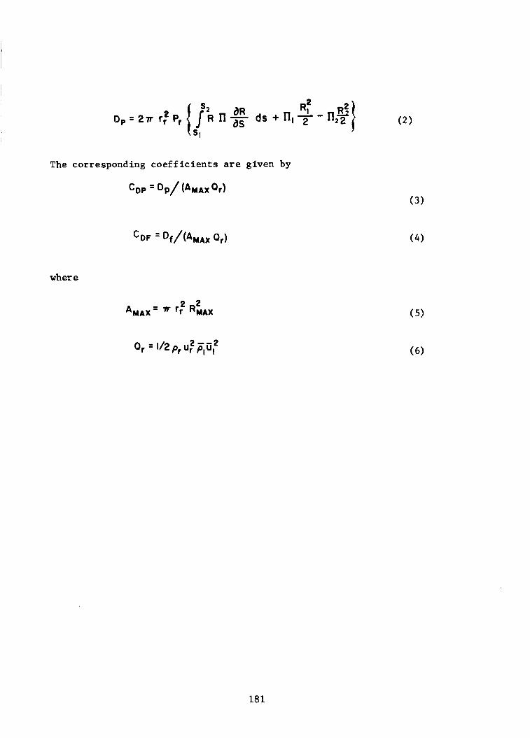
The corresponding coe f f i c i ent s are given by
cop = ~ p / (AMAX or)
where
181

Subrout ine PERFN2
Object Compute i n v i s c i d n a c e l l e drag
Opt i o n s
None
L i s t of Symbols
DPR = D , Pressu re d r a g P
P = P , S t a t i c P r e s s u r e
P1, P2 = P 1 J 2 , S t a t i c p r e s s u r e (P/Pr) a t p re sc r ibed s t a t i o n s
R 1 , R2 = R1, R2 , Nacelle r a d i u s (r l /rr) a t p re sc r ibed s t a t i o n s .
s = s , Streamwise coord ina te .
S19S2 = SIPS2 , Streamwise coord ina te a t p r e s c r i b e d s t a t i o n .
Theory
I n terms of t h e d imens ionless v a r i a b l e s used i n t h e a n a l y s i s , t h e p r e s s u r e drag is g iven by;
182
Subrout ine PdIS (RESM, ITER) I
Object - I
Solve Poisson equa t ion I
01) t ion
IDBGP = 0 No debug p r i n t o u t = 1 P r i n t o u t r e s i d u a l s = 2 P r i n t s o l u t i o n
L i s t of Symbols
P(K, J>
F(K, J>
PSI(K)
ITER
RLX
RESMAX
RESDM
RESM
Theory
J,
c\r
J,
V
€MAX
M E
E
, Stream f u n c t i o n (d imens ionless )
, C o e f f i c i e n t (l/PG) - (d imens ionless )
, I t e r a t i v e guess f o r J
, I t e r a t i o n counter
Relaxa t ion f a c t o r
, Maximum r e s i d u a l accepted
, Maximum r e s i d u a l / J s t a t i o n
9 Maximum res idua l / sweep
The s o l u t i o n a lgo r i thm is desc r ibed i n Reference 1.
- References
1. Anderson, 0. L. and D. E. Edwards: Extension t o a n Analys is of Turbulent Swi r l ing Compressible Flow i n Axisymmetric Ducts, NASA Contrac t NAS3-21853, 1981, UTRC Report R81-914720.
183

Subrout ine P0 ISCF
Object
(1) ( 2 ) (2)
Se t of c o e f f i c i e n t s of $ 9 = o S e t boundary c o n d i t i o n s on J, S e t i n i t i a l guess f o r JI
Options
IDBG17 = 0 Compressible Flow = 1 Incompressible Flow
IDBGT = 0 No debug tes t case = 1 Debug tes t case
IDBGP = 0 No debug tes t p r i n t o u t = 1 Debug p r i n t o u t
Variables
Q ( I : K )
FIV ( I, L, K)
0
V
G
V
P
0
,Coord ina te f u n c t i o n s
,Dependent v a r i a b l e s €o r i n v i s c i d f low
,Stream f u n c t i o n a t s t a t i o n J
, C o e f f i c i e n t f o r a$/a n
, C o e f f i c i e n t of p2 J,
, C o e f f i c i e n t f o r v e l o c i t y c a l c u l a t i o n
, Density r a t i o (P/P,)
,Temperature r a t i o (T/Tr)
,Metric c o e f f i c i e n t d imens ionless
,Gap ( g / r r >
,Metric c o e f f i c i e n t (d imens ionless )
,Densi ty r a t i o (p/P,)
Temperature r a t i o (T/T,)
,Upstream cons tan t v e l o c i t y (uo/ur)
184

I USINF I 1 UPINF
PS IKL
TEMINF
RXOINF
AMINF
PTINF
BLK
Subroutine POISCF (Cont'd)
, F r e e stream a x i a l v e l o c i t y (uSw/Ur)
,Free stream t a n g e n t i a l v e l o c i t y u + , / u r
,Free stream stream f u n c t i o n (d imens ioniess )
,Free stream s t a t i c tempera ture r a t i o (T/Tr)
,Free stream d e n s i t y r a t i o (Pip,)
,Free stream Mach number
,Free stream t o t a l p r e s s u r e r a t i o (P,/P,)
,see COMMON/SPCGD/
Theory
Th i s s u b r o u t i n e does t h e fo l lowing s teps
(1) Reads c o o r d i n a t e Q f i l e and s o l u t i o n FIV f i l e ( 2 ) I n t e r p o l a t e s t h e s o l u t i o n t o t h e (rl,S) g r i d ( 3 ) C a l c u l a t e s t h e c o e f f i c i e n t F = 1/PG ( 4 ) ( 5 ) S e t s boundary c o n d i t i o n on Y ( 6 ) C a l c u l a t e s i n i t i a l guess f o r \y
(7 ) S t o r e s F, BLK, P on d i s k f i l e s
Calculates c o e f f i c i e n t s BLK f o r s t r e a m l i n e c u r v a t u r e c a l c u l a t i o n
The i n i t i a l guess is g iven by t h e i n v i s c i d s o l u t i o n obta ined from CALINV. The boundary c o n d i t i o n s are g iven by:
J I ( 0 , S ) = 0
185

Subrout ine P 0 I S@N
Object
C a l c u l a t e axisymmetric s t r e a m l i n e c u r v a t u r e
Options
IdPT7 = 0 No c u r v a t u r e c o r r e c t i o n s
= 1 Curvature c o r r e c t i o n
I D B G 1 5 = 0 Use i n p u t KL s t r e a m l i n e s
> 0 Use I D B G 1 5 streamlines
L i s t o f Symbols
IRH0 ,Densi ty i t e r a t i o n counter
ITERL ,Maximum number of i t e r a t i o n s
KHdLD ,No. ADD code s t r e a m l i n e s
KL ,No. SCURVA s t r e a m l i n e s
RESMAX ,Maximum r e s i d u a l f o r convergence
Theory
This s u b r o u t i n e i s a c a l l i n g subrout ine f o r s u b r o u t i n e s INTFRE, P@ISCF, PgIS, and SCURVA.
186
Subrout ine QINTER
I Object
I n t e r p o l a t e c u r v a t u r e from PdIS mesh to SdLVI mesh I t
Op t i o n s ~ -
I None
L i s t of Symbols I --
Q ( J , K ) Coordinate f u n c t i o n s
Theory
A f t e r t h e c u r v a t u r e and flow ang le has been c a l c u l a t e d from t h e p o t e n t i a l flow s o l u t i o n , . t h i s s u b r o u t i n e i n t e r p o l a t e s t o o b t a i n v a l u e s a t t h e numerical g r i d p o i n t s which w i l l be used i n t h e SbLVI c a l c u l a t i o n .

Subrout ine FXADPF(J,JJ)
Object
Read P and F f i l e s i n NIST word b locks
Option
None
L i s t of Symbols
J J
JJ JJ
N N
F F
P l4.J
NST = 25
NBK
NIST
NFDRM
NL
NBIST
NMOVE
= 23
,Record number
,Record number i n b lock N
,Block number
2 , C o e f f i c i e n t s of V $J = 0
, Stream f u n c t i o n (d imens ionless )
,Number of r e c o r d s p e r b lock
,Number of words t o move p o i n t e r
,Number of words p e r b lock
, C o e f f i c i e n t f i l e number F a r r a y
,Last b lock number
,Number of words f o r two r eco rds
,Number of words t o move p o i n t e r
Theory
The e n t i r e F and P a r r a y s cannot be kep t i n co re a t t h e same t i m e so t h a t t h e 1/0 is arranged t o keep f i x e d b locks i n c o r e (F ig . 1). Let (J,K) be a p o i n t on t h e computational mesh and (JJ,KK) t h e cor responding p o i n t i n core . L e t each record be t h e J t h l i n e w i t h t h e number of words i n t h e r eco rd g iven by
K = 1,IST
I f t h e r e are NST r e c o r d s p e r b lock , then t h e s e are NIST words p e r b lock ,
NIST = NST x I S T
188

Subrout ine E A D P F ( J , J J ) (Cont 'd)
-- Theory (Cont'd)
The s o l u t i o n a l g o r i t h m r e q u i r e s over lapping b locks as shown on F ig . 1. I
Hence w e have t h e b lock number
N = (5-2) /(NST-2) +- 1
and t h e JJ p o i n t i n c o r e i s g iven by
JJ + J-(N-1) x (NST-2)
This s u b r o u t i n e i s coded s o t h a t a new block is ready only when N = NL.
189

Subrout ine FEADPG(J,JJ)
Object
Read v a r i a b l e f o r c u r v a t u r e c a l c u l a t i o n
Options
None
List o f Symbols
J
JJ
N
G
P
NST
NBK
NIST
NGDRM
NPDRM
NL
NBIST
NGIST
NGL
Theory
= J ,Record number
= JZ ,Record number i n b lock N
,Block number
,S t reaml ine coord ina te d a t a (see COMMON/SPCFD/)
,Stream f u n c t i o n
= 25 ,Number of r eco rds p e r b lock
,Number of words t o move p o i n t e r
,Number of words p e r P b lock
= 25 ,Unit number of G a r r a y
= 24 ,Unit number f c r P a r r a y
, L a s t P b lock number
,No. words f o r 2 P reco rds
,No. words f o r 2 G r e c o r d s
,Last G record number
This subrou t ine r eads t h e P f i l e accord ing t o Subrout ine R W P F bu t r eads on ly t h e J t h G r eco rd which i s kep t i n co re .
190

Function RGSRTS(C,ETA,LflP)
Compute d i s t o r t e d mesh u s i n g Roberts ' t r ans fo rma t ion
Opt i o n s
L@P = 0 Wall - w a l l boundary = 1 Wall-free stream boundary =-1 Free stream-wall boundary
L i s t o f Symbols
c = c , D i s t o r t i o n parameter
ETA = r~ , Inpu t v a r i a b l e (uni f orm mesh)
LOP = , Op t i o n
Output Var i ab le
RPBRTS = n ,Output v a r i a b l e
Theory --
The Rober t s ' t r ans fo rma t ion f o r a d i s t o r t e d mesh on both s i d e s i s g iven by
.. I + exp[2 In(-) c+ 1/2 (+ 1/2)]
where
For t h e d i f f e r e n t o p t i o n s we have
e -7 J
191

Subrout ine RQUND
Object Round c o r n e r s on s t r a i g h t w a l l duc t s .
L i s t of Symbols
XM , Axial l o c a t i o n
IWALL I n d i c a t e s Rub o r Tip Wall
DX S t e p s i z e i n x d i r e c t i o n
I n sub rou t ine GDUCT, i f t h e op t ion I0PT3’ 8 i s used then a s t r a i g h t w a l l i s cons t ruc t ed between i n i t i a l d a t a p o i n t s . d i s c o n t i n u i t y between w a l l segments t h i s sub rou t ine is used t o round o r smooth ou t t h e d i s c r e t e r e p r e s e n t a t i o n s of t h e w a l l i n order f o r i t t o appear smooth.
Thus i n o rde r t o remove
Subrout ine SLETE(KSSLE,KSSTE)
Object Find b l ade c o n t r o l s u r f a c e s .
Options
None.
L i s t of Symbols
KSSLE,KSSTE
SLE, STE
ZLEH , ZLET
ZTEH, ZTET
Leadtng edge and t r a i l i n g edge index
, Leading and t r a i l i n g edge c o o r d i n a t e s (dimensionless)
, Axial d i s t a n c e hub l e a d i n g and t r a i l i n g edge (dimensionless)
, Axial d i s t a n c e t i p l e a d i n g and t r a i l i n g edge (dimensionless)
Theory
The i n t e r s e c t i o n of t h e l ead ing and t r a i l i n g edge of t h e b l a d e w i t h t h e hub and t i p cas ing are obta ined from Subrou t ine GBLADE. of t h e hub and t i p boundar ies are searched u n t i l t h e proper v a l u e of streamwise
Then the c o o r d i n a t e s
192

coord ina te s f o r t h e l ead ing edge and t r a i l i n g edge of t h e b l ade a re found. The coord ina te index KSSLE is l o c a t e d j u s t upstream of t h e b l ade and t h e
I I
I ~ coord ina te KSSTE is l o c a t e d j u s t downstream of t h e b lade .
193
Subroutine SCURVA (IDBU,KH@LD)
Object
Calculate curvature from potential flow solution
IDBU = 0 Update density I > 0 Print SCURVA solution, update curvature I
Variables
KHOLD ,No. ADD code streamlines
,No. SCURVA streamlines KL
Q(J,K) ,Coordinate functions
P (K) ,Stream function a station J (dimensionless)
G (K) G ,Coefficient for velocity calculation
R(K) P ,Density Ratio (p/pr) (dimensionless)
us ,Streamwise velocity (dimensionless)
UN Un ,Normal velocity (dimensionless)
U U ,Total velocity (dimensionless)
COSTH cos2 ( 0 ) of flow angle e
,Curvature of streamline (dimensionless) av an
CURV -
Theory
Once the potential flow solution has been obtained from subroutine P@IS, this subroutine will calculate the flow angle and streamline curvature according to Ref. (1).
References
1. Anderson, O.L. and D. E. Edwards, Extension to an Analysis of Turbulent Swirling Compressible Flow in Asixymmetric Ducts, NASA Contract No. NAS3-21851, 1981, UTRC Report R81-914720. I
I
194

I Subrout ine SM@@TH (X,J,JX,XB,YB,JXB,JXK)
I i Object Least squa res s p l i n e f i t smoothing f o r geometry
I Opt ions
None
L i s t of Symbols
= XJ
= YJ
= XJ
= YJ
-
-
= Y J
= C(1,J)
= YK
Theory
, Number of i npu t p o i n t s
, Number of ou tput p o i n t s
, Number of s p l i n e knots
, Input p o i n t s a b s c i s s a
, Input p o i n t s o r d i n a t e
, Output p o i n t s a b s c i s s a
, Output p o i n t s o r d i n a t e
, Second d e r i v a t i v e of Y(X)
, S p l i n e c o e f f i c i e n t s
, Constants of Integration
This sub rou t ine computes t h e second d e r i v a t i v e of t h e inpu t vec to r Y(X). With t h e use of t h e s tandard math package ISML r o u t i n e s , ( r e f e r e n c e 9) i t then f i t s a least square s p l i n e t o t h e second d e r i v a t i v e wi th JXK movable knots . ou tput s o l u t i o n v e c t o r ?(Ti) a t JXB p o i n t s . r o u t i n e s ICSFKU, ICSFKV, UERTST.
The s p l i n e equat ions are then i n t e g r a t e d a n a l y t i c a l l y t o o b t a i n t h e Subrout ine SM88TH uses ISML
195

Subrout ine SdLVI
Object I n t e g r a t e equa t ions of motion f o r v i scous flow.
Opt ions
None
L i s t of Svmbols
= aIJ
= bIJ
- ‘IJ
= dIJ
-
= k I J - l ) K
= eIJ
= 9 1
= ZT
= cf$H
= ‘f4T
= ‘fSH
= ‘fST
, Element of x mat r ix
, Element of E mat r ix
, Element of E mat r ix
, Element of 5 mat r ix
, Element of b” m a t r i x
, Element of Ek m a t r i x
, Element of 6 mat r ix
, Element of Zk mat r ix
, Stress c o e f f i c i e n t hub (25.,4/(F1i1 ) )
, Stress c o e f f i c i e n t t i p ( - 2 ~ n 4 / ( ~ 1 ~ 1 ) )
, Stress c o e f f i c i e n t hub (2~,,/(P1E1 ) )
, Stress c o e f f i c i e n t t i p (-2EnS/(FlEl2))
2
2 - -
2
=
= E(1) , Truncat ion e r r o r (IT)
1 / 4 ( p Ul2) , Mean i n l e t dynamic p r e s s u r e (dimensionless)
- , Mean i n l e t en t ropy = I1
= E(.rr) , Truncat ion e r r o r (IT)
= €(PO) , Truncat ion e r r o r (PO)
= E(PUS) , Truncat ion e r r o r (PUS)
196

EUPUP
EUSUS
PIREF
PI0
PRCEF
PSIHl, PSIH2
PSITl, PSIT2
QAVE
QWALH
QWALT
QPLUS
SIG
SIGWH
S IGWT
STAH
?TAT
THETA0
TPLUS
TWH,TWT
U
UPLUS
USH,UST
J J-1 = *,%-I
= PTUT *3
= Q/(PU*3)
= €
= w H
=%I
= ' tH
- ' tT -
= eo
= + T
2
2
, Truncat ion e r r o r (Uq, )
, Truncat ion e r r o r (Us )
, Mean i n l e t r e f e r e n c e p r e s s u r e (dimensionless)
, T o t a l p r e s s u r e (d imens ionless )
, Local p r e s s u r e c o e f f i c i e n t (dimensionless)
, Wall stream f u n c t i o n (hub) (d imens ionless )
, Wall stream f u n c t i o n ( t i p ) (dimensionless)
, I n l e t energy f l u x (dimensionless)
, Energy f l u x (hub) (d imens ionless )
, Energy f l u x ( t i p ) (dimensionless)
, Universa l hea t f l u x (d imens ionless )
, S t r e s s (dimensionless)
, Wall stress (hub) (d imens ionless )
, Wall stress ( t i p ) (dimensionless)
, Stanton number (hub) QH/ [Pus (eo+) 3
, s t a n t o n number ( t i p ) QT/[PUS(8,-8) I
, T o t a l temperature (dimensionless)
, Universa l stress (dimensionless)
, Wall tempera ture (hub, t i p ) (d imens ionless )
, Magnitude of v e l o c i t y (dimensionless)
, Unive r sa l v e l o c i t y (dfmensionless)
, F r i c t i o n v e l o c i t y (hub, t i p ) (d imens ionless )
-- -
- - -
197

XMACH = M , Mach number (dimensionless)
YPLUS I y+ , Universal distance (dimensionless)
Z = z , Axial distance (dimensionless)
zz = zs , Axial distance to next s l o t (dimensionless)
Theory
The equations of motion are solved using the method derived i n
reference 6 . A flow diagram i s shown i n Fig. 24.
198

Subrout ine STRESI
Object Compute i n i t i a l stress d i s t r i b u t i o n
Options
LdP=1 S t o r e i n l e t flow stress L(dP+l
L i s t of Svmbols Do n o t s t o r e i n l e t flow stress
See C@MMQ)N b lock v a r i a b l e s i n s u b r o u t i n e l i s t i n g s .
Theory
The i n i t i a l stress and h e a t f l u x d i s t r i b u t i o n is computed from
199

Subrout ine STRT
Obi ect Find i n l e t f low l o c a t ion
OD t ion
None
L i s t of Symbols
ZINLET
SINLET
INLET
Theory
, Axial i n l e t f low l o c a t i o n
, Streamwise i n l e t f low l o c a t i o n
, Counter
Once t h e ax-a1 l o c a t i o n of t h e ,.ilet f low -s determined t h e streamwise l o c a t i o n may be found s i n c e t h e a x i a l l o c a t i o n a t each p o i n t i n t h e coord ina te system is p a i r e d wi th its streamwise coord ina te .
Subrout ine TPRINT
Object Calls CPU t i m e .
200

Subrout ine TURB
Object Compute t u r b u l e n t v i s c o s i t y
Options
N@PT=O I n i t i a l t u rbu lence model N@PT=l Subsequent t u rbu lence model
L i s t of Symbols
AMUE
AMLJER (K)
AMUM
AMLJW
AMUW
AMLJO
DEL0
DU
DUDZ
E
EM
=,m
ENP
ENS
EW
PHI
R H ~ M
= AU
= dU/dZ
Turbulent v i s c o s i t y (d imens ionless )
Freestreant t u r b u l e n t v i s c o s i t y (dimensionless)
Freestreant molecular v i s c o s i t y (d imens ionless )
Wall v a l u e of molecular v i s c o s i t y (dimensionless)
Mole cu l a r v i s co s it y (d imens ion less )
Maximum f r e e s t r e a m v i s c o s i t y (d imens ionless )
Displacement t h i c k n e s s (d imens ionless )
Ve loc i ty f i n i t e - d i f f e r e n c e (d imens ionless )
Veloc it y d e r i v a t ive (d imens i o n l e s s )
Rate of s t r a i n (d imens ionless )
S t r a i n f r e e s t r e a m (d imens ionless )
S t r a i n huh, t i p , edge of i n n e r l a y e r (dimen- s i o n l e s s )
Swi r l rate of s t r a i n (d imens ionless )
Streamwise ra te of s t r a i n (d imens ionless )
Wall rate of s t r a i n (d imens ionless )
Turbulence model f u n c t i o n (dimensionless)
Densi ty f ireestream (dimens ionless )
20 1

SIGWH
SIGWK
S IGWT
TPLUSl, TPLUS2
USTARH, USTART
Y
YK
yMH,m
YPLUSl, YPLUS2
+ + = T T 1' 2
= UK
= uoD
= u ,u * * H T
= Y
= 'k.tZlz
= YH,YT
+ + 1' 2
= Y Y
, Wall stress(hub)(dimensionless)
,
, Wall stress ( t i p ) (dimensionless)
Wall stress ( inner l a y e r ) (dimensionless)
, Universa l w a l l stress (d imens ionless )
, Magnitude of v e l o c i t y (d imens ionless )
, Freestream v e l o c i t y (d imens ionless )
, F r i c t i o n ve loc i ty (hub , t i p ) (d imens ionless )
, Distance a c r o s s duc t (d imens ionless )
, Dis tance a c r o s s duc t (d imens ionless )
, Dis tance t o inne r l a y e r h u b , t i p ) (d imens ionless )
, Universa l d i s t a n c e (d imens ionless )
Theory
The tu rbu lence model i s desc r ibed i n r e f e r e n c e (1) and t h e r e s u l t i n g equa t ions are desc r ibed below. t i n u o u s f u n c t i o n
L e t t h e eddy v i s c o s i t y be desc r ibed by a con-
- - - +E PE Pr
where
E = J-
and
20 2

NRp~uwn* (outer layer)
E M + =
% where y i s t h e d i s t a n c e from t h e w a l l
L
Y = I Y - Y w l (5)
A matching p o i n t f o r t h e i n n e r l a y e r and o u t e r l a y e r e x i s t s f o r each w a l l denoted Y o u t e r l a y e r
and YT and w i t h a cor responding s t r a i n EH and ET. Then f o r t h e H
The t u r b u l e n t v i s c o s i t y and thermal c o n d u c t i v i t y is g iven by
F T P +E - = - + - Pr Pr Pr (7 )
The t u r b u l e n t f l ow p r o p e r t i e s can be c a l c u l a t e d a t s t a t i o n J-1 because t h e f low f i e l d i s known. For s t a t i o n J , i t i s noted that t h e t u r b u l e n t v i s c o s i t y is a s t r o n g f u n c t i o n of stress, t h u s from equa t ion (l),
where
Hence,
20 3

and
+ + I F i n a l l y , i t is noted t h a t a t t h e i n i t i a l s t a t i o n T (Y i n equat ion .3
i s no t known, t h e r e f o r e , T+ = 1 is assumed.
204

Function UBLAS
Object
Options
C a l c u l a t e v e l o c i t y r a t i o accord ing t o t h e B l a s i u s s o l u t i o n f o r t h e i n i t i a l flow.
None
Theory
The v e l o c i t y r a t i o i s de termined .by i n t e r p o l a t i o n s of d a t a b lock con- t a i n i n g B l a s i u s s o l u t i o n t o t h e f low p a s t an axisyrnmetric shape ( r e f e r e n c e 10).
205

Funct ion UCflLES (Argument L i s t )
Object Find f r i c t i o n v e l o c i t y f o r t h e i n i t i a l p r o f i l e from Coles law
Opt i o n s
None
L i s t of Symbols
AK = k
- - vw ANUW
DELT = 6
DELTS = 6*
DERR = dE/dU*
ERR = E
ERRM = E
ITER = l J
ITERL = l J
UINF = u m
us = (U*p
1 us1 I = (U*)
Theory
The f r i c t i o n v e l o c i t y i s ob ta ined from Coles l a w us ing Newton's method
Von Karman cons t an t (dimensionless)
2 Kinematic v i s c o s i t y ( f t / s ec )
Boundary l a y e r t h i c k n e s s ( f t )
Displacement t h i c k n e s s ( f t )
Slope of e r r o r f u n c t i o n (d imens ionless )
E r ro r f u n c t i o n (d imens ionless )
, Convergence c r i te r ia (d imens ionless )
I terate
Maximum number of i t e r a t i o n s
Freestream v e l o c i t y ( f t / s e c )
, Guess f o r f r i c t i o n v e l o c i t y ( f t / s e c )
, I n i t i a l guess f o r U* ( f t / s e c )
206

Convergence occur s when
I E p I c E
20 7

Subrout ine WAKC6R
Object Compute n a c e l l e wake c o r r e c t i ons .
Options
None
L i s t of Svmbols
AMl,AM2
DRL
DZL
ETA
~ ( 1 , J, L)
G (2 , J , L)
G ( 3 , J,L)
G ( 4 , J,L)
G ( 5 , J, L)
G ( 6 , J,L)
RL
SL I
S2,Sl
T@T1, T@T2
T 1 , T2
u1, u2
us1, us2
UP1, UP2
VL
, I n v i s c i d f low Mach number Mk-l' Mk
, Radia l wake c o r r e c t i o n ARL
, Axia l wake c o r r e c t i o n AzL
?I , Normal coord ina te
+L , Wake distance (radians)
, Tangen t i a l wake c o r r e c t i o n
P a r t i a l d e r i v a t i v e 9
a A $ / as P a r t i a l d e r i v a t i v e
AR , Radia l wake c o r r e c t i o n
AZ , Axial wake c o r r e c t i o n
RL
SL
, Radia l l o c a t i o n of l i f t i n g l i n e s t r e a m l i n e
, S coord ina te of l i f t i n g l i n e s t r e a m l i n e
'J * 'J-1 , S coord ina te of mesh
( T o / T ) ~ , T o t a l t o s t a t i c tempera ture r a t i o
, S t a t i c tempera ture T K - l ' TK
= VL
, I n v i s c i d f low v e l o c i t y
, I n v i s c i d f low streamwise v e l o c i t y
, I n v i s c i d f low t a n g e n t i a l v e l o c i t y
, Metric scale c o e f f i c i e n t of Lth s t r e a m l i n e
208

ZL
J
, Axial d i s t a n c e Lth s t r e a m l i n e
, Index of S coord ina te
K , Index of N coord ina te
L , Index of L s t r e a m l i n e Theory To o b t a i n t h e c o r r e c t i o n s t o t h e wake geometry due t o t h e nace l le ' s p resence i n t h e flow f i e l d , t h i s s u b r o u t i n e i n t e g r a t e s t h e fo l lowing equa t ions . ( formulted i n r e f e r e n c e 1 ) .
t h
SJ
9 (SJ,RL) = R J (1) US"
L
us ing t h e t r a p e z o i d r u l e a long t h e s t r e a m l i n e s pas s ing through t h e p o i n t (RL, ZL) o r (SL,n L) . The remaining wake c o r r e c t i o n s are given by
b R L = RL(SJI - RL
"a = 2, CsjI - 2, (sL) -
Labeled Common Blocks Used i n The Nacel le P o r t i o n
( 3 )
Included h e r e i n is an a l p h a b e t i c a l l i s t of t h e -abeled common b-oc s used i n t h e nacelle p o r t i o n of t h e a n a l y s i s and a d e s c r i p t i o n of each v a r i a b l e used i n them.
COMMON BLOCK NAME DESCRIPTION OF (OBJECT) VARIABLE NAME VARIABLES
AC0NS (Blade Data - CdNSTI (1, L) = RCL Radius of p r o p e l l e r l i f t i n g Dimensional ized) 1 i n e
C6NSTI ( 2 , L) = as
C0NSTI ( 3 , L) = B Chord
Stagger a n g l e
C0NSTI ( 4 , L) = t / B Thickness
C@NSTI (5 , L) Not used
CQNSTI (6, L) = ZcL Axial l o c a t i o n of p r o p e l l e r l i f t i n g l i n e
20 9

Subrout ine WBLEED
Object
Ca lcu la t e p e r f o r a t e d w a l l b leed
Opt ions
IgPT18 = 0 = 1 = 2 = 3
PCHEK > 1 .0 < 1 . 0
No w a l l b leed T ip w a l l b l eed Hub w a l l b leed Tip/hub w a l l b l eed
Flow e n t e r s t unne l Flow l e a v e s tunne l
Input Var i ab le s
AHAS = \ /As Rat io of h o l e area t o s u r f a c e area
C D I S H = C Discharge c o e f f i c i e n t
PTP = PTp Plenum t o t a l p r e s s u r e
TTP = TT Plenum t o t a l t empera ture
I n t e r n a l Var i ab le s
MITU
GAXMA
GASR
PS
PT
P STL'
PTTU
TSTU
TTTU
RH@R
U SR
PRESR
- - MTU = Y
= R
= P
= PT
- - 'TTU
- *TU
- T~~~
- -
- -
- c - r
r
- 'r
= u -
Tunnel Mach number
Ra t io of s p e c i f i c h e a t s
Gas c o n s t a n t
S t a t i c p r e s s u r e ( p s f a )
T o t a l p r e s s u r e ( p s f a )
Tunnel s t a t i c p r e s s u r e ( p s f a )
Tunnel t o t a l p r e s s u r e (ps fa )
Tunnel s t a t i c tempera ture (deg R)
Tunnel t o t a l t empera ture (deg R) 3
Reference d e n s i t y ( s l u g / f t )
Reference v e l o c i t y ( f t / s e c )
Reference p r e s s u r e ( p s f a )
210
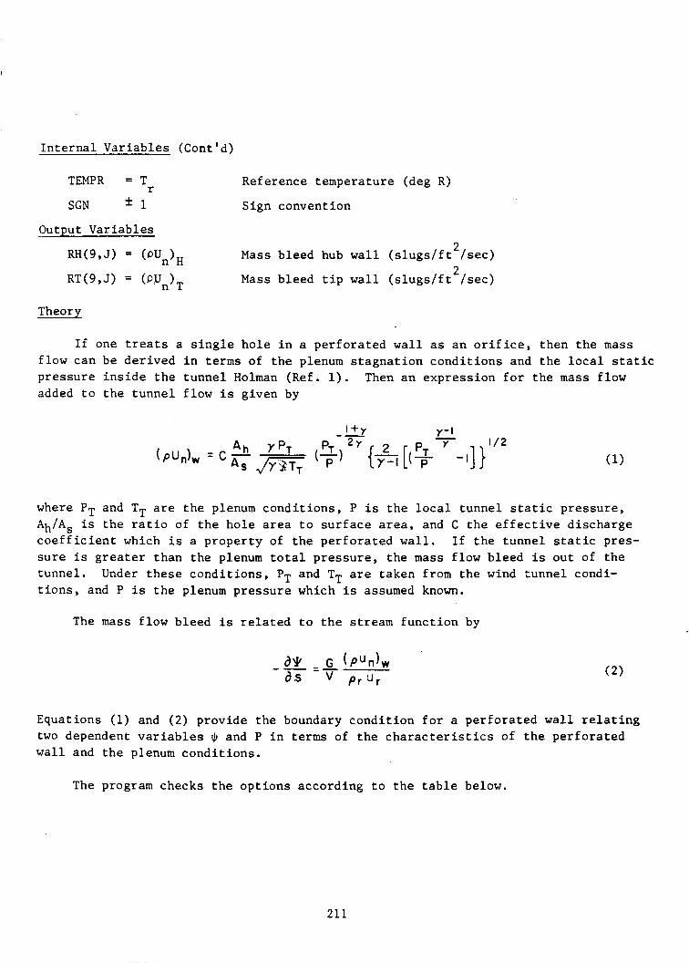
I n t e r n a l V a r i a b l e s (Cont’d)
TEMPR = T Reference tempera ture (deg R)
SGN f l Sign convention r
Output Var i ab le s 2
2 RH(9, J ) = Mass b leed hub w a l l ( s l u g s / f t / s ec )
RT(9,J) = Mass b leed t i p w a l l ( s l u g s / f t / s e c )
Theory
I f one t rea ts a s i n g l e h o l e i n a p e r f o r a t e d w a l l as a n o r i f i c e , t hen t h e mass flow can be de r ived i n terms of t h e plenum s t a g n a t i o n c o n d i t i o n s and t h e l o c a l s t a t i c p r e s s u r e i n s i d e t h e t u n n e l Holman (Ref. 1). Then a n expres s ion f o r t h e mass flow added t o t h e t u n n e l f low i s g iven by
where PT and TT are t h e plenum c o n d i t i o n s , P i s t h e l o c a l t unne l s t a t i c p r e s s u r e , Ah/As i s t h e r a t i o of t h e h o l e area t o s u r f a c e area, and C t h e e f f e c t i v e d i scha rge c o e f f i c i e n t which is a p r o p e r t y of t h e p e r f o r a t e d w a l l . I f t h e tunne l s t a t i c pres - s u r e is g r e a t e r than t h e plenum t o t a l p ressure , , t h e mass flow b leed is ou t of t h e tunne l . t i o n s , and P is t h e plenum p r e s s u r e which is assumed known.
Under t h e s e c o n d i t i o n s , PT and TT are taken from t h e wind tunne l condi-
The mass f low b leed is r e l a t e d t o t h e stream f u n c t i o n by
Equations (1) and ( 2 ) p rovide t h e boundary c o n d i t i o n f o r a p e r f o r a t e d w a l l r e l a t i n g two dependent v a r i a b l e s $ and P i n terms of t h e c h a r a c t e r i s t i c s of t h e p e r f o r a t e d wa l l and t h e plenum c o n d i t i o n s .
The program checks t h e o p t i o n s accord ing t o t h e t a b l e below.
211
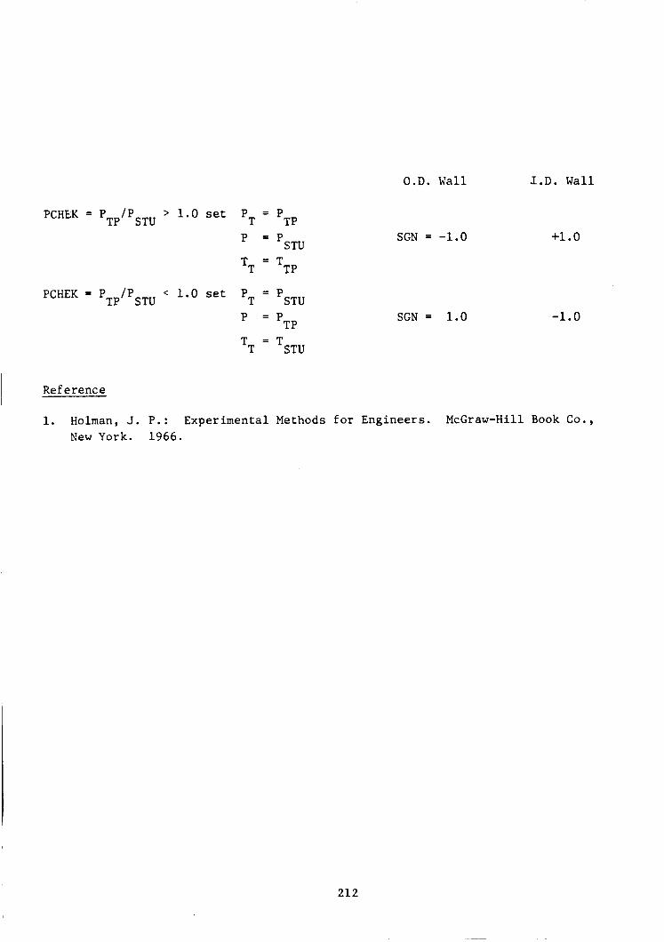
- 'T - 'TP PCHEK = P / P > 1 .0 set TP STU
STU P = P
TP
STU
TT = T
PCHEK = PTp/PsTu < 1.0 se t PT = P
P = PTP
O.D. Wall
SGN = -1.0
SGN = 1.0
I.D. Wall
+1.0
-1.0
I Reference
1. Holman, J. P . : Experimental Methods f o r Engineers. McGraw-Hill Book Co., New York. 1966.
212

Subroutine WRITPF( J J )
Object
S t o r e updated p o t e n t i a l f low s o l u t i o n .
Opt i o n s
None
L i s t of Symbols
JJ
:TST
NIST
NPDRbi = 24
P
Theory
The s t ream f u n c t i o n a r r a y P(JJ,KK) i s ar ranged i n c o r e as desc r ibed i n sub rou t ine READPF, Fig. 1. When an i t e r a t ive sweep of one b lock is complete, t h e new updated s o l u t i o n is w r i t t e n on a d i s k f i l e . when JJ = NST-1.
Th i s occurs
, J J t h s t a t i o n i n co re
,No. r e c o r d s p e r block
,No. words p e r b lock
, Uni t number
,Stream func t ion
213

Function XH ( J )
Object C a l c u l a t e w a l l l e n g t h on I D w a l l
Va r i ab le s
J
XH
Theory
AxH
Wall p o i n t no.
Wall l e n g t h
Function XT(J)
Objec t C a l c u l a t e w a l l l e n g t h on OD w a l l
Var i a b l es
J
XT
Theory
Wall p o i n t no.
Wall l e n g t h AxT
214
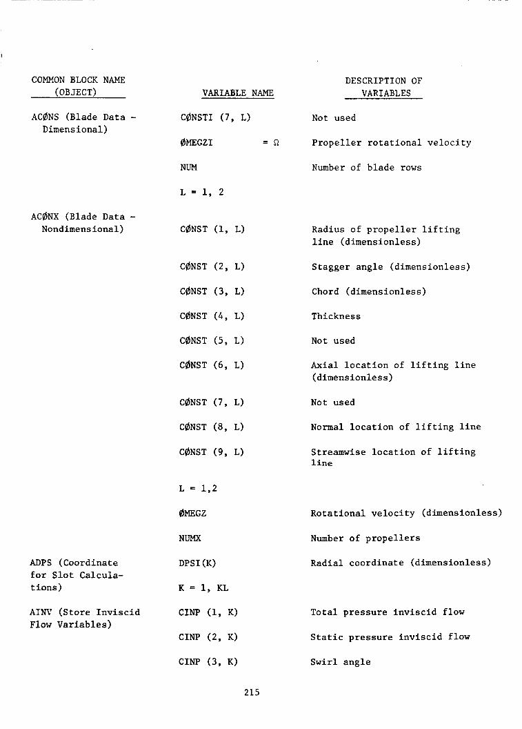
COMMON BLOCK NAME (OBJECT)
ACdNS (Blade Data - Dimensional)
ACdNX (Blade Data - Nondimensional)
ADPs (Coordinate for Slot Calcula- tions)
AT" (Store Inviscid Flow Variables)
VARIABLE NAME
CdNSTI (7 , L)
dMEGZI = R
NUM
L = l , 2
CdNST (1, L)
CdNST (2 , L)
CdNST (3 , L)
CdNST ( 4 , L)
CdNST (5, L)
CdNST (6, L)
CdNST ( 7 , L)
CdNST (8, L)
CdNST (9, L)
L = 1,2
dMEGZ
NUMX
DPSI (K)
K = 1, KL
CIN" (1, K)
CINP ( 2 , K)
CINP ( 3 , K)
DESCRIPTION OF VARIABLES
Not used
Propeller rotational velocity
Number of blade rows
Radius of propeller lifting line (dimensionless)
Stagger angle (dimensionless)
Chord (dimensionless)
Thickness
Not used
Axial location of lifting line (dimensionless)
Not used
Normal location of lifting line
Streamwise location of lifting l i n e
Rotational velocity (dimensionless)
Number of propellers
Radial coordinate (dimensionless)
Total pressure inviscid flow
Static pressure inviscid flow
Swirl angle
215

I COMMON BLOCK NAME (OBJECT)
AKK (Complex Coor- d i n a t e)
AMATRX (Matr ix Inver - s ion )
APLgT ( S t o r e Var i ab le s f o r P l o t t i n g )
BCPIX (Complex Vari- a b l e s )
VARIABLE NAME
CINP (4, K)
K = 1, KL
M 1
M 2
W(2, J) = ZT
W ( 5 , J ) = CFSH
FST W(6, J) = C
A(1 , I ) = Ai
A(2 , I ) = bi
'i A(3 , I ) =
A(4, I ) = ri
DESCRIPTION OF VARIABLES -
Tota l temperature i n v i s c i d flow
Flags f o r DEBUG p r i n t o u t
See Subrout ine FCPLX
Element of D ma t r ix
Element of D-' ma t r ix
Axial d i s t a n c e (hub) (dimen- s i o n l e s s )
Axial d i s t a n c e ( t i p ) (dimension- less)
P r e s s u r e c o e f f i c i e n t (hub) (dimens i o n l e s s )
P r e s s u r e c o e f f i c i e n t ( t i p ) (d imens ionless )
F r i c t i o n c o e f f i c i e n t (hub) ( d h e n s i o n l ess )
F r i c t i o n c o e f f i c i e n t ( t i p ) (d h e n s i o n l e s s )
Source s t r e n g t h (d imens ionless )
Loca t ion of p o l e (d imens ionless )
Wall a n g l e change (deg)
Radius i n z p lane (dimension- less)
Angle i n z p l a n e ( r a d i a n s )
R e l a t i v e x d i s t a n c e i n z p lane (d imens ionless )
216

COMMON BLOCK NAME (OBJECT) VARIABLE NAME
BCPLX (Complex V a r i - - b l e s ) A(7,I) = Yi
B( l , I ,K) = ASXs
B(2,J,K) = ASYs
B(3,I,K) = ASSs
B(4,I,K) = AS,,,
X(1,K) = S
X ( 2 , K ) = n
X(3,K) = X
X(4,K) = Y
X(6,K) = n
X(8,K) = ‘1,
CESCRIPTION OF VARIABLES
R e l a t i v e Y d i s t a n c e i n z plane (d imens ionless )
Change i n coord ina te x (dimen- s i o n l e s s 1
Change i n coord ina te y (dimen- s i o n l e s s )
Change i n coord ina te 6 (dimen- s i o n l e s s )
Change incoord ina te rl (dimen- s i o n l e s s )
Streamwise coord ina te (dimen- s i o n l e s s )
Norma 1 coord ina te (d imens ion- less)
X coord ina te i n z p l a n e (dimen- s i o n l e s s )
Y coord ina te i n z p lane (dimen- s i o n l e s s )
5 - coord ina te i n w p l ane (dimen- s i o n l e s s )
, , -coordinate i n w p l ane (dimen- s i o n l e s s )
Streamwise d e r i v a t i v e of 5 ( d imens i o n l e s s)
Streamwise d e r i v a t i v e of n (dimensionless)
21 7

COMMON BLOCK NAME (OBJECT)
BLEED ( w a l l b l eed )
X(10,K) = Y(S+AS)
X(11,K) = C(S+DS)
X(13,K) = Y
X(16,K) = Vn
X(17,K) = Vs
AHAS = \/As
CDISH = C
PTP = PTp
TTP = TT
DESCRIPTION OF VARIABLES
Coordina tes a t s t a t i o n S+DS
Coordinates a t s t a t i o n S+DS
Coordinates a t s t a t i o n S+DS
Coordinates a t s t a t i o n S+DS
Metric scale c o e f f i c i e n t s (dimensionless)
Second d e r i v a t i v e of 6 (dimensionless)
Cross d e r i v a t i v e of 5 (dimen- s i o n l e s s )
Normal d e r i v a t i v e of V (dimen- s i o n l e s s )
Streamwise d e r i v a t i v e of V (d imens ionless )
Ra t io of h o l e area t o s u r f a c e area
Discharge c o e f f i c i e n t
Plenum t o t a l p r e s s u r e
Plenum t o t a l temperature
BTHIK
, Number of p o i n t s
, F r a c t i o n a l chordwise d i s t a n c e
9 Thickness/ Chord = yI
218

COMMON BLOCK NAME (OBJECT) VARIABLE NAME
P CCPU (Parameters NPTS = N
I f o r Complex Trans- form)
NS0URC = Ns
!&DER1 = O1
O2 0RDER2 =
!&DER3 = O3
SLO = SL0
XDS = S
XDN = S
DESCRIPTION OF VARIABLES
Number of s i n g u l a r i t i e s i n complex t r a n s f otmat i on
Number of sou rces i n z plane
Absolute magnitude of l a r g e s t term
Absolute magnitude of l a r g e s t term
Absolute magnitude of l a r g e s t term
Length of streamwise coord ina te
S tep s i z e f o r complex i n t e g r a - t ion
Step s i z e f o r complex i n t e g r a - t ion
219

COMMON BLOCK NAME (OBJECT)
CINF (Parameters for Poisson Equation)
VARIABLE NAME
AMINF - Mw
DEDN(K) = (dn/dn)k
DZEDN(K) = (d211/dn2)k
PINF = n w
PSIKL - $w
PTINF
RH0INF
R~TLNF
TEMINF
TTLNF
UINF
UPINF
US INF
UUO
wo
= p w
= Po-
= ow
= @ow
W = u
= uo
= vo
DESCRIPTION OF VARIABLES
Freestream Mach number
Transverse coordinate
Transverse coordinate stretching
Transverse coordinate stretching
Freestream static pressure (dimensionless)
Freestream stream tunctlon (dimensionless) Freestream total pressure (dimensionless) Freestream density (d imenslonless) Freestream total density (dimensionless) Freestream static temperature (d h e n s ionl es s ) Freestream total temperature (dimensionless) Freestream velocity (dimensionless) Freestream tangential velocity (dimensionless) Freestream streamwise velocity (dimensionless) Reference velocity (dimensionless)
Reference metric coefficient
2 20

I COMMON BLOCK NAME (OBJECT) VARIABLE NAME
I
I C@NST (Flow Constants) A C H I = x AKAPPA =
APLUS =
CPR =
I
CVR =
EP =
GAMMA =
GASR =
GRAVR
P I =
PRESR =
PRL =
PRT =
RHgR =
SNDR =
TEMPR =
T I
VISCR =
K
A
C
+
P r
C v r
O e
a
R -
IT
'r Pr
P r
'r
L
T
C r
T r
"r
DESCRIPTION OF VARIABLES
Clauser c o n s t a n t (0.016)
von Karman c o n s t a n t (0.41)
van Driest c o n s t a n t (26.0)
S p e c i f i c h e a t a t cons tan t p r e s s u r e (5997.0 f t 2 / s e c 2 / d e g R)
S p e c i f i c h e a t a t cons tan t volume (3283.0 f t 2 / sec2 /deg R)
2 .7182818
R a t i o of s p e c i f i c h e a t s (1 .4)
Gas c o n s t a n t (1714.0 f t 2 2 /set deg R)
G r a v i t a t i o n a l c o n s t a n t s (32.2 f t / s e c ) 2
3.1415926
Reference s t a t i c p r e s s u r e (psfa )
P r a n d t l number laminar 0.70
P r a n d t l number t u r b u l e n t 0.72
Reference d e n s i t y ( s l u g s / f t 3
Reference speed of sound (1116.0 f t / s e c )
Reference temperature (deg Raukine)
(0.1745329 rad ians /deg)
Reference molecular v i s c o s i t y (0.370 x
221

COMMON BLOCK NAME (OBJECT)
CPRE (Coordinate I Func t ions )
VARIABLE NAME
Q ( 1 , K ) = R
Q ( 2 , K ) = Z
Q ( 3 , K ) = aR/an
Q ( ~ , K ) = a R / a s
DESCRIPTION OF VARIABLES
Radius (dimensionless)
Axia l d i s t a n c e (dimensionless
Normal d e r i v a t i v e of r a d i u s (dimensionless)
S t r e a m w i s e d e r i v a t i v e of r a d i u s (d imens ionless )
Second d e r i v a t i v e of r a d i u s (dimensionless)
Metric s c a l e c o e f f i c i e n t ( d i m en s ion 1 e s s )
Curvature of p o t e n t i a l l i n e (d imens ionless )
Curva ture of s t r e a m l i n e (d imens ionless
Second d e r i v a t i v e of metric scale c o e f f i c i e n t (d imens ionless )
P h y s i c a l d i s t a n c e a c r o s s duc t (d imens ionless )
F r a c t i o n a l d i s t a n c e a c r o s s duc t (d h e n s i o n l e s s )
Area between ad jacen t stream- l i n e s (d imens ionless )
Gap between b l ade s u r f a c e s (d h e n s i o n l e s s )
Normal d e r i v a t i v e of b lade s u r f a c e (d imens ionless )
222

I [ COMMON BLOCK NAME I (OBJECT) I
I
DESCRIPTION OF VARIABLE NAME VARIABLES
I
Q(15,K) = a G / a S St reamwise d e r i v a t i v e of b l ade s u r f a c e (d imens ionless )
I
Q(16,K) = a d a n Transform of normal coord ina te (d imens ionless )
Second d e r i v a t i v e (dimensionless) 2 ~ ( 1 7 , ~ ) = a n / an2
Q(18,K) = n Normal coord ina te (d h e n s ion 1 e s s)
Transformed normal coord ina te (d imens ionless )
K = l , K L Number of s t r e a m l i n e s (dimensionless)
223

COMMON BLOCK NAME DESCRIPTION OF (OBJECT) VARIABLE NAME VARIABLES
CORE 2* (Wall Value of Coordinate Funct ions) Rg(1,K) = R Radius (dimensionless)
RQ(2,K) = dR/dZ D e r i v a t i v e of r a d i u s (dimen- s i o n l es s )
Second d e r i v a t i v e of r a d i u s (d imens i o n l e s s )
Rg(3,K) = d2R/dZ2
RP(4,K) = Z Axia l d i s t a n c e (d imens ionless )
RQ(5,K) = V Metr ic s c a l e c o e f f i c i e n t (dimensionless)
Rg(6,K) = dY/dS D e r i v a t i v e of metric s c a l e c o e f f i c i e n t (d imens ionless )
Rg(7,K) = YT Dis t ance a c r o s s duc t (dimen- s i o n l e s s )
Rg(8,K) = S Streamwise c o o r d i n a t e (dimen- s i o n l e s s)
Mass f low b leed (d imens ionless ) 0 R0(9,K) = m
R @ ( ~ o , K ) = O w Wall tempera ture (d imens ionless )
RgS(1) = Rg(1,K) Dummy Storage Vector
I * Note: Ac tua l ly t h r e e a r r a y s def ined where $? t a k e s on t h e v a l u e H, M , T
8 = H, Hub w a l l
= M , ?lean l i n e
= T , Tip w a l l
DERIV (Force Funct ions) DF(1,K) = bs/xV]i+ Streamwise b l ade force/volume (dimensionless)
Tangen t i a l b l ade force/volume (dimensionless)
DF(2,K) = [H+/XV]i,
T o t a l p r e s s u r e loss/volume ( d h e n s i o n l e s s )
224

COMMON BLOCK NAME (OBJECT)
DRED1 ( S t o r e Flow V a r i a b l e s )
DRED2 ( S t o r e Flow V a r i a b l e s )
DUC0UT (Wall Coordinates)
VARIABLE NAME
DF(5,K) = [HiW]J-l K-%
B L ~ C K (I)
I1 = 1 9 * KL + 35
I = 1, I1
B L ~ C K ~ (I)
R(2 ,3 , J ) = 61T(ZJ)
DESCRIPTION OF VARIABLES
Coordina te d i s t o r t i o n (d imens ionless )
Streamwise b l a d e f orce/volume (d imens ionless )
Tangen t i a l b l ade force/volume (dimens i o n l e s s )
T o t a l p r e s s u r e loss/volume (d imens ionless )
Coordina te d i s t o r t i o n (dimen- s i o n l e s s)
Grid s t r u c t u r e v a r i a b l e s
Grid s t r u c t u r e v a r i a b l e s
Radius of hub (d imens ionless )
Radius of t i p (d imens ionless )
Mass f low of t i p b l eed (dimension- less)
Mass f low of hub b l eed (dimen- s i o n l e s s
Wall tempera ture of t i p (d imens ionless )
Wall t empera tu re of hub (dimens i o n l e s s )
Axial l o c a t i o n of hub
Axial l o c a t i o n of t i p

COMMOh' BLOCK NAME (OBJECT)
DESCRIPTION OF VARIABLE NAME VARIABLES
DUCTIN (Input Functions) BINI(L) = BINPUT(I,J,K) , see C@MM@N/SPI@/
I = 1,5
J = 1,2
K = 1,KLL
L = 5*(K-l)+I+(J-l)*5*KLL
DUCTI(1) I = 1,15 , Arbitrary duct geometry parameters
RD~I(L) = R(l,l,L)*RADR , Tip wall coordinates (ft)
RD2I(L) = R(1,2,L)*RPDR , Hub wall coordinates (ft)
ZDlI(L) = R(1,4,L)*RADR , Tip wall coordinates (ft)
ZD2I(L) = R(2,4,L)*RADR , Hub wall coordinates (ft)
L = 1, JL
DUCTIX (Input Functions) AINI (L) = AINDUCT (I,J,K) , See C@MM@N/SPI@X/
L = 1, JL
EBLAD (Blade Row N R ~ W Parameter)
, Number of Streamwise stations
, Maximum number of propeller Rows
LRBW , Indicates propeller row
LBLD , Not used
NBLADE 9 Number of blades in propeller row
226

COMMON BLOCK NAME (OBJECT)
FC4)R (Truncation Error Estimates)
i VARIABLE NAME
= E v a
EAS = %s
EEN = EI
EPO = Epo
$ ESI = E
ET0 = ETO
DESCRIPTION OF VARIABLES
Error in swirl velocity (d hens ionles s )
Error in streamwise velocity (dimensionless)
Error in entropy (dimensionless)
Error in total pressure (dimensionless)
Error in stream function (dimensionless)
Error in total temperature (dimensionless)
227

COMMON BLOCK NAME BESCRIPTION OF (OBJECT) VARIABLE NAME VARIABLES
FIVC (Inviscid Flow FIV(1,L.K) Jr
FIV(Z,L,K) = U Variables I/O)
5
FIV(3,L.K) = u$
FIV(4,L.K) = n
FIV(5,L.K) = I
FIV(6,L,K) = 8
FIV(7,L.K) = P
Stream function (dimensionless)
Streamwise velocity (dimensionless) Tangential velocity (d hens ionless) Static pressure (dimensionless)
Entropy (dimensionless)
Stat ic temperature (d h e n s ionles
Density (dimensionless)
M Mach number FIV(8,L,K) - FIV(9,L.K) =
FIV(10,L.K) =
L=1 @ J-1station
L=2 @ J station
L=3 @ J+1 station
K=l,KL streamlines
FIPARM(1) 'r
FIPARM(2) = Tr
FIPARM(3) = pr
FIPARM(4) - 8
FIPARM(8) = R
3 Reference density (slugs/ft
Reference temperature (deg R)
Reference pressure (psfa)
Gravita t ional constant ( f t / sec
Reference viscosity (slugs/ft/sec)
Specific heat constant pressure (f t2/sec2/deg) Specific heat constant volume ( f t2 / aec2/deg) Cas constant (ft 2 2 /sec /deg)
228
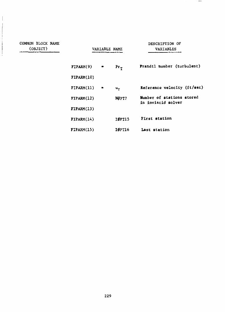
COMMON BLOCK NAME (OBJECT
FIPARM(9)
FIPAFLM ( 10)
FIPARM(11)
FIPARM(1Z)
FIPARM(13)
FIPARM( 14)
FIPARM( 15)
DESCRIPTION OF VARIABLE NAME VARIABLES
Prandtl number (turbulent) T =
Reference velocity ( f t / sec) U Y t
N0PT7 Number of s tat ions stored In inviscid solver
First station 10PT15
IbPT16 Last st at ion
229
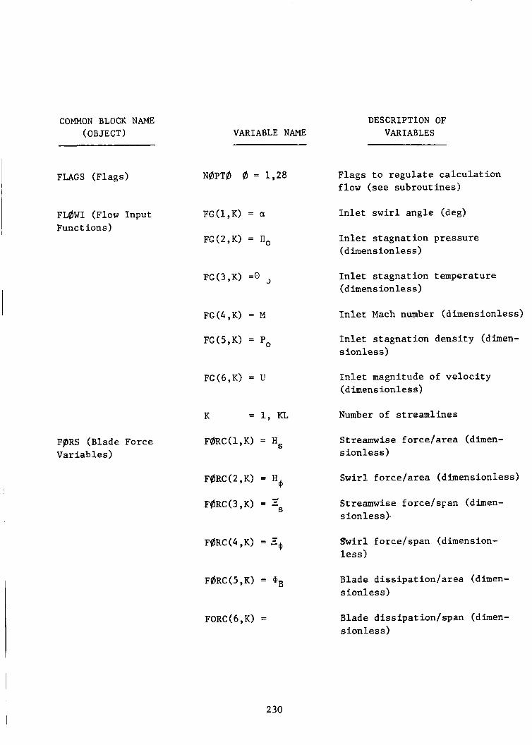
COMMON BLOCK NAME (OBJECT 1 VARIABLE NAME
DESCRIPTION OF VARIABLES
FLAGS (Flags)
FL@WI (Flow Input Funct ions)
FPRS (Blade Force V a r i a b l e s
N@PTb b = 1,28
F G ( ~ , K ) = a
FG(2,K) = no
FG(3,K) =o
FG(4,K) = M
FG(5,K) = Po
FG(6,K) = U
K = 1, KL
FdRC(1,K) = Hs
@ F@RC(2,K) = H
FbRC(3,K) = Ls -
FORC(6,K) =
Flags t o r e g u l a t e c a l c u l a t i o n f low ( s e e sub rou t ines )
I n l e t s w i r l a n g l e (deg)
I n l e t s t a g n a t i o n p r e s s u r e (dimens i o n l e s s )
I n l e t s t a g n a t i o n tempera ture (d imens ionless )
I n l e t Mach number (d imens ionless )
I n l e t s t a g n a t i o n d e n s i t y (dimen- s i o n l e s s )
I n l e t magnitude of v e l o c i t y (d imens ionless )
Number of s t r e a m l i n e s
Streamwise f o r c e / a r e a (dimen- s i o n l e s s )
S w i r l f o r c e / a r e a (d imens ionless )
Streamwise fo rce / sFan (dimen- s i o n l e s s ) .
Swirl fo rce / span (dimension- l e s s )
Blade d i s s i p a t i o d a r e a (dimen- s i o n l e s s )
Blade d i s s i p a t i o n / s p a n (dimen- s i o n l e s s )
230

C O ~ I O N BLOCK rim (OBJECT)
FORS2 (Blade Force Var iab les )
VARIABLE NNlE
A FF( l , I ,K) = M
A FF(2,I,K) =
A FF(3,I ,K = 8
A FF(4,I,K) 8,
A FF(5,I,K) = no
A FF(6,I,K) = P
A FF(7,I,K) = Us
A FF(8,1,K) = U+
A F F ( ~ , I , K ) = \?+
FF(~O,I ,K) = uB
FF(II,I,K) = a
A
A
A FF(12,I,K) = B
A FF(13,I,K) = I
A FF(14,1,K) = U
231
DESCRIPTION OF VARIABLES
I n v i s c i d Mach number (dimen- s i o n l e s s )
I n v i s c i d s t a t i c p r e s s u r e (d imens ionless )
I n v i s c i d s t a t i c tempera ture ( d h e n s i o n l e s s )
I n v i s c i d t o t a l t empera ture (dimension1 ess )
I n v i s c i d t o t a l p r e s s u r e (dimensionless)
I n v i s c i d d e n s i t y (dimen- s i o n l e s s )
I n v i s c i d streamwise v e l o c i t y (dimensionless)
Absolute s w i r l v e l o c i t y (d imens ionless )
Relative s w i r l v e l o c i t y (dimensionless)
S l a d e v e l o c i t y (dimen- s i o n l e s s )
Absolute a n g l e t o axis (deg)
R e l a t i v e a n g l e t o axis (deg)
I n v i s c i d f low entropy (dimensionless)
Magnitude of r e l a t i v e i n v i s c i d f low v e l o c i t y (dimensionless)
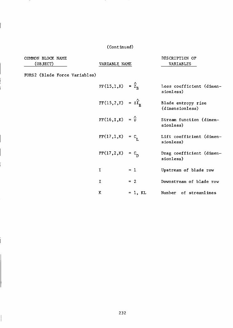
(Cont h u e d )
COMMON BLOCK NAPE (OBJECT) VARIABLE NAME
FORS2 (Blade Force Var i ab le s )
A FF(15,I,K) = ZB
h FF(15,2,K) = A I B
A FF(16,1,K) = $
FF(17,1,K) - - cL
FF(17,2,K) = CD
I = 1
I = 2
K = 1, KL
DESCRIPTION OF VARIABLES
Loss c o e f f i c i e n t (dimen- s i o n l e s s )
Blade en t ropy r ise (d imens ionless )
Stream f u n c t i o n (dimen- s i o n l e s s )
L i f t c o e f f i c i e n t (dimen- s i o n l e s s )
Drag c o e f f i c i e n t (dimen- s i o n l e s s )
Upstream of b l ade row
Downstream of b l a d e row
Number of s t r e a m l i n e s
232

COMMON BLOCK NAME (OBJECT) VARIABLE NAME
K = 1 ,KL
FUNC (Dependent Flow F ( l , I y K ) = ifi V a r i a b l e s )
F(2 , I ,K) = Us
F(3 , I ,K) = UQ
F(4,I ,K) = JI
F(5 , I ,K) = I
F(6,I ,K) = 0
F(7 , I ,K) = P
F(8,I,K) = Ens
I
I
K
INTINP ( I n t e g e r Input I0PT0 V a r i a b l e s )
IDBG@
ISHAPE
J L
KDS
KL
= 1
= 2
= 3
= 1, KL
= 1, 17
= 1, 23
DESCRIPTION OF VARIABLES
Number of s t r e a m l i n e s (dimen- s i o n l e s s)
Stream f unc t ion (d imen s ion 1 e s s )
S t r eamw is e v e l oc i t y ( d imen s ion - l e s s )
Swi r l v e l o c i t y (d imens ionless )
S t a t i c p r e s s u r e (d imens ionless )
Entropy (d imens ionless )
S t a t i c tempera ture (dimension- less)
Dens i ty (d imens ionless )
S t r e a m w i s e stress (dimension- less)
Swi r l stress (d imens ionless )
Heat f l u x (d imens ionless )
I n l e t c o n d i t i o n s
s= s
S= S+d S
Number of s t r e a m l i n e s
Input/Output o p t i o n s
Debug p r i n t o u t o p t i o n s
Blade shape o p t i o n
Number of streamwise s t a t i o n s
Number of s t e p s p e r streamwise s ta t i o n
Number of S t r eaml ines
233

COMMON BLOCK NAME DESCRIPTION OF (OBJECT) VARIABLE NAME VARIABLES
KLL Number of input data streamlines
NB Number of blades
INTPAR (Parameter Variables)
These variables are treated as PARAMETER statements in UNIVAC programs and as integer variables in IBM or CDC programs.
I Parameters for Solution Arrays
PARAMETER IST = 1 0 PARAMETER IS = 100 PARAMETER NEQ = 10 PARAMETER NBCH = 5 PARAMETER NBCT = 5 PARAMETER NBHl = NBCH+1 = 6 PARAMETER NEQD = 2*NEQ = 20
Parameters for Slots
PARAMETER ISLPT = 15 PARAMETER ISLpT2 = 2*ISLfJT = 30 PARAMETER IS1 = 6*ISLpT+2 = 92 PARAMETER IS2 = 2*IS+IS1 = 292
Parameters for Coordinate Arrays
PARAMETER ISM = 19*IST = 1900 PARAMETER ISL = ISM+35 = 1935 PARAMETER IS3 = ISM+2 = 1902 PARAPiETER IS4 = IS3+10 = l a 2 PARAMETER IS5 = IS4+10 = 1922 PARAMETER IS6 = IS5+10 = 1932
Parameters for Matrix Inversion
PARAMETER KKLP = 30 PARAMETER LNGTg = NEQ*NEG*KKLP+NEQ*KKLP = 3300 PARAMETER LNGTl = NEQ*NEQ*KKLP+l = 3001 PARAMETER LNGT2 = 2"LNGTO = 6600 PARAMETER LNGT3 = 3*IST*NEQ = 3000
234
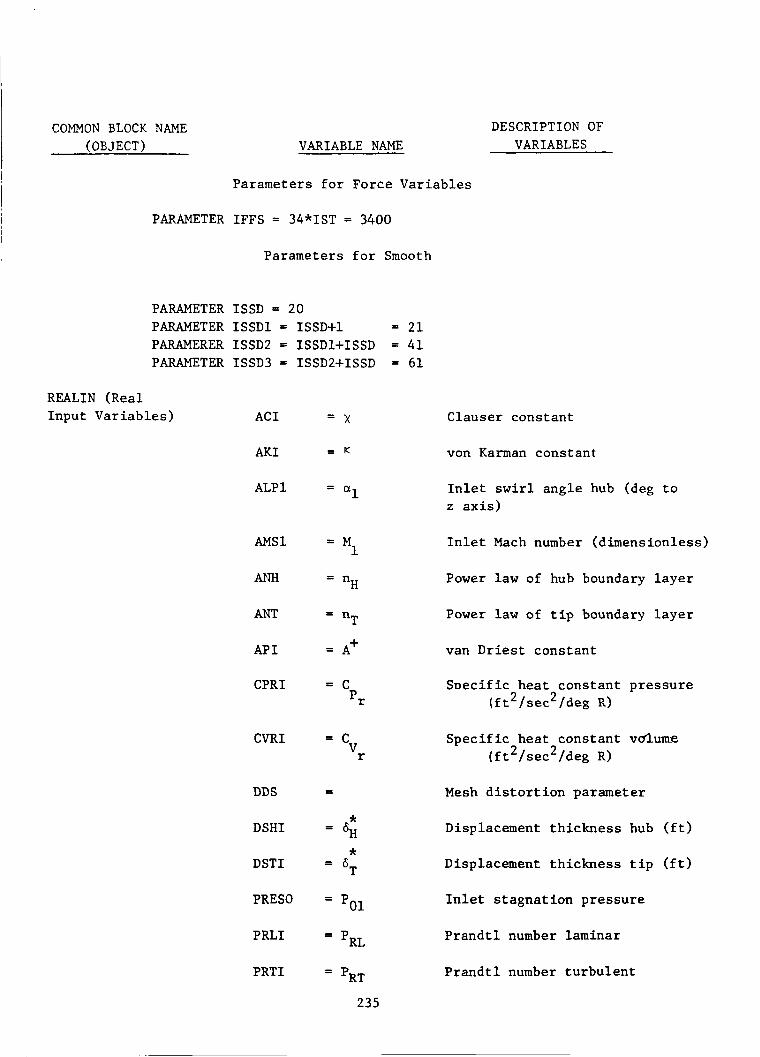
COMMON BLOCK NAME (OBJECT) VARIABLE NAME
DESCRIPTION OF VARIABLES
Parameters f o r Force V a r i a b l e s
PARAMETER IFFS = 34*IST = 3400
Parameters f o r Smooth
PARAMETER ISSD = 20 PARAMETER I S S D l = ISSD+1 = 2 1 PARAMERER ISSD2 = ISSDl+ISSD = 4 1 PARAMETER ISSD3 = ISSD2+ISSD = 6 1
REALIN (Real I n p u t V a r i a b l e s ) AC I = x Clauser cons tan t
A K I = K von Karman constant
ALP1 = a1
AMs 1 = M1
I n l e t s w i r l a n g l e hub (deg t o z a x i s )
I n l e t Mach number (dimensionless)
A” = nH Power l a w of hub boundary l a y e r
ANT = nT Power l a w of t i p boundary l a y e r
API = A+ van Driest c o n s t a n t
CPRI = c SDecif i c h e a t c o n s t a n t p r e s s u r e pr (f t2 / sec2/deg R)
C V R I = cv S p e c i f i c h e a t c o n s t a n t vdlume r ( f t2 / sec2/deg R)
DDS = Mesh d i s t o r t i o n parameter
DSHI = 6H Displacement t h i c k n e s s hub ( f t )
DSTI = 6T Displacement t h i c k n e s s t i p ( f t )
* *
PRES0 = Pol I n l e t s t a g n a t i o n p r e s s u r e
PRLI = Pu P r a n d t l number laminar
P r a n d t l number t u r b u l e n t = P~~ PRTI
235

COMMON BLOCK NAME (OBJECT) VARIABLE NAME
T E P P 0
VISCRI
REALIX (Real Input ALPHSI V a r i a b l e s )
ALPSMI
ALPSTI
C0RDIII
C0RDMI
CBRDTI
PHICHI
PHICMI
PHI CT I
RCLHI
RCLMI
RCLTI
THIKHI
= T o 1
- 'r -
= 'CH
- - aCM
= 'CT
= BH
- - BP
= BT
- 'CH
- 'CM
- 'CT
= r
-
-
-
CLH
= r CLM
CLT = r
= t H / B H
DESCRIPTIOR OF VARIABLES
I n l e t s t a g n a t i o n tempera ture (deg R)
Molecular v i s c o s i t y r e f e r e n c e ( l b / s e c f t
3
Blade s t a g g e r a n g l e hub (deg t o z a x i s )
Blade s t a g g e r a n g l e mid (deg t o z a x i s )
Blade s t a g g e r a n g l e t i p (deg t o z a x i s )
Blade chord hub ( f t )
Blade chord midpoint ( f t )
Blade chord t i p ( f t )
Blade camber hub (deg)
Blade camber midpoint (deg)
Blade camber t i p (deg)
Hub r a d i u s of b l a d e c e n t e r l i n e ( f t )
Midpoint r a d i u s of b l a d e c e n t e r - l i n e ( f t )
Tip r a d i u s of b l a d e c e n t e r l i n e ( f t )
Blade t h i c k n e s s t o chord r a t i o hub (dimensionless)
236

DESCRIPTION OF VARIABLES
COMMON BLOCK NAME (OBJECT) VARIABLE NAME
Blade t h i c k n e s s t o chord r a t i o midpoint (dimensionless)
Blade t h i c k n e s s t o chord r a t i o t i p (d imens ionless )
= 'CLH Blade Axial l o c a t i o n of c e n t e r - l i n e (Hub)
= zcLM Blade a x i a l l o c a t i o n of c e n t e r - l i n e (Midpoint)
Blade a x i a l l o c a t i o n of c e n t e r - l i n e (Tip)
Blade c e n t e r l i n e l o c a t i o n ( f t )
SPCFD (Var iab les i n Poisson Equat ion)
C o e f f i c i e n t s of Poisson equa t ion
J = YK S t r e a m func t ion
SPCGD (Var iab les f o r S t reaml ine Curvature)
C o e f f i c i e n t of Poisson equa t ion
C o e f f i c i e n t f o r v e l o c i t y
Densi ty r a t i o (pip,)
Temperature r a t i o (T/Tr)
Metric c o e f f i c i e n t
Average a x i a l l o c a t i o n (dimen- s i o n l e s s )
SPIb (Flow Var i ab le s ) AC'E(1,J) =
Area r a t i o (dimensionless) AVE(2,J) = AR
Mass flow (dimensionless) -
AVE(4,J) = Us Average streamwise v e l o c i t y (dimens i o n l e s s )
- =
AVE ( 5 , J ) Average s w i r l v e l o c i t y (d imens ionless )
23 7

COMMON BLOCK NAME (OBJECT) VARIABLE NAME
AVE(6,J) = ll
- AVE(7,J) = I
- AVE(~,J) = P
- AVE(10,J) = M
AVE(11,J) = Eo
AVE(12,J) = go
- AVE(13,J) = Cp
AVE(15,J) = 2
AVE(16,J) = B
% AVE(17,J) = M
J = 1, JL
BINPUT(I,J,K) = Y
BIMPUT(2, J,K) = ITo
BINPUT(3,J,K) = ll
BII?PUT(4,J,K) = a
DESCRIPTION OF VARIABLES
Average entropy (dimensionless)
Average entropy (dimensionless)
Average static temperature (dimensionless)
Average density (dimensionless)
Average Mach number (dimen- s ionles s)
Average total pressure (dimen- s ionless)
Average total temperature (dimensionless)
Average pressure coefficient (dimensionless)
Average total pressure loss (dimensionless)
Diffuser effectiveness (dimen- sionless)
Blockage ( d hens ion 1 e s s )
Area average Mach number (dimensionless)
Spanwise location (dimension- less)
2 Total pressure (lb/ft abs)
Static pressure (lb/ft abs) 2
Swirl angle (deg to axis)
238

COMMON BLOCK NAME (OBJECT)
DESCRIPTION OF VARIABLE NAME VARIABLES
BINPUT(5,J,K) = eo Total temperature (deg R)
J = l Inlet flow
J = 2 Exit flow
K = 1, KLL Number of spanwise stations
SPIdX (Flow Variables) AINPUT(l,J,K) = Y Spanwise location (dimensionless)
2 AINPUT(2,J,K) = no Total pressure (lb/ft abs)
AINPUT(3,J,K) = I'I Static pressure (lb/ft abs) 2
AINPUT(4,J7K) = a Swirl angle (deg to axis)
AINPUT(5,J,K) = Oo Total temperature (deg R)
J = l Upstream of blade row (dimen- sionless)
J = 2 Downstream of blade row (dimen- s ionless)
K = 1, KLL Number of spanwise stations
STRMES (Poisson BP@IS = B Stretching parameter Stretching Parameter)
BPgISI = BI Input stretching parameter
239

COMMON BLOCK NAME (OBJECT) VARIABLE NAME
STRES (Funct ions of G(1,K) = [G/V];-+ Orthogonal Coordinates)
DESCRIPTION OF VARIABLES
--I-
G ( ~ + I , K ) = G(1,K) @ J-1, I=1 ,9 K : 1,KL
SVARB (Parameters ALPHS = a Stagger a n g l e t o a x i s (deg) and V a r i a b l e s )
ALPLUM = No t used i n t h i s v e r s i o n
AMACHR = K Reference Mach number (dimen- r s i o n l e s s)
- AMACHl = M1 Average i n l e t Mach number
(dimensionless )
AMPLUM = Kot used i n t h i s v e r s i o n
AMPLUS = M+ Mass f low b leed parameter (dimensionless)
- APRESl = P1
AREA1 = A1
Ar ARFAR =
Average i n l e t s t a t i c p r e s s u r e (d h e n s i o n l e s s )
I n l e t area ( f t 2 )
Reference area ( f t 2
240
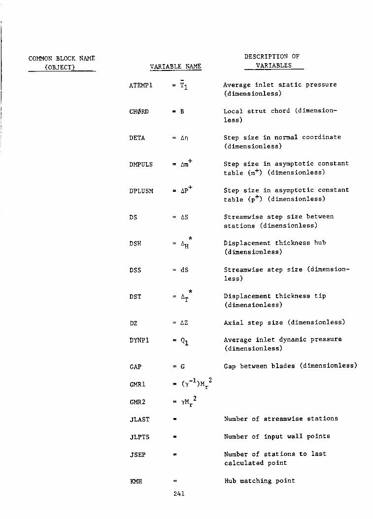
DESCRIPTION OF VARIABLES
COMMON BLOCK NAME (OBJECT) VARIABLE NAME
ATEMP 1
CHgRD
DETA
DMPULS
DPLUSM
DS
D SH
DSS
DST
DZ
DYNP 1
GAP
G M R l
GMR2
JLAST
JLPT S
JSEP
KMH
Average i n l e t s t a t i c p r e s s u r e ( d h e n s i o n l e s s)
Local s t r u t chord (dimension- l e s s )
= B
Step s i z e i n normal c o o r d i n a t e (dimensionless)
= A n
+ = Am Step s i z e i n asymptot ic c o n s t a n t t a b l e (m') (dimensionless)
= AP+ Step s i z e i n asymptot ic c o n s t a n t t a b l e (p') (dimensionless)
= AS Streamwise s t e p s i z e between s t a t i o n s (dimensionless)
* = AH Displacement t h i c k n e s s hub
( d h e n s i o n l e s s )
Streamwise s t e p s i z e (dimension- less)
= dS
* = AT Displacement t h i c k n e s s t i p
(dimens i o n l e s s )
Axial s t e p s i z e (dimensionless) = AZ
Average i n l e t dynamic p r e s s u r e (dimensionless)
Gap between b l a d e s (dimensionless) = G
= (y-')Mr2
2 = YMr
Number of streamwise s t a t i o n s
Number of i n p u t w a l l p o i n t s
Number of s t a t i o n s t o l a s t c a l c u l a t e d p o i n t
Hub matching p o i n t - - 24 1

COMMON BLOCK NAME (OBJECT) VARIABLE NAME
KMT
KMO
KSEP
LM
LMM
PHIC
PLUSM
PPLUS
RADR
REY
RHdR
SL
s0m
THICK
USTARH
USTART
U SR
WFLd
YPLUSM
DESCRIPTION OF VARIABLES
Tip matching point
Not used in this version
Not used in this version
Size of table of constants for inner layer (dimensionless)
Midpoint of table of constants for inner layer (dimensionless)
Blade camber (deg)
Not used in this version
Pressure gradient parameter (dimensionless)
Reference radius of blade centerline (dimensionless)
Reynolds number P R U /U
Reference density (slugs/ft )
r r r r 3
Length of duct in streamline coordinates (dimensionless)
Solidity (dimensionless)
Lmal blade thickness (dimen- sionless)
Friction velocity hub (dimen- sionless)
Friction velocity tip (dimen- sionless)
Reference radius (dimensionless)
Weight flow (lb/sec)
Matching point for table asymptotic constants (dimension- less)
242
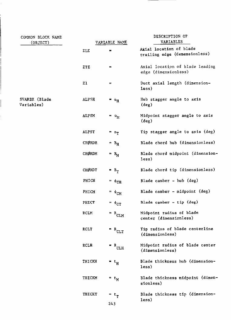
COMMON BLOCK NAME (OBJECT)
SVARBX (Blade V a r i a b l e s )
VARIABLE NAME
ZLE
ZTE
z 1
ALP SH
ALP SM
ALPST
CH0RDH
CH0RDM
CHgRDT
PHICH
PHICM
PHICT
RCLM
RCLT
RCLH
THICKH
THICKM
THICKT
=
- -
- -
= a H
= a14
= aT
= BH
= %
= BT
= 'CH
= 'CM
= 'CT
= R CLM
CLT = R
= R CLH
= tH
= tM
= tT
243
DESCRIPTION OF VARIABLES
Axial l o c a t i o n of b l a d e t r a i l i n g edge (demens i o n 1 ess )
Axial l o c a t i p n of b l a d e l e a d i n g edge (dimensionless)
Duct a x i a l l e n g t h (dimension- less)
Hub s t a g g e r a n g l e t o a x i s (deg)
Midpoint s t a g g e r a n g l e t o a x i s (deg)
Tip s t a g g e r a n g l e t o a x i s (deg)
Blade chord hub (dimensionless)
Blade chord midpoint (dimension- less)
Blade chord t i p (dimensionless)
Blade camber - hub (deg)
Blade camber - midpoint (deg)
Blade camber - t i p (deg)
Midpoint r a d i u s of b l a d e c e n t e r (dimensionless)
Tip r a d i u s of b l a d e c e n t e r l i n e (dimensionless)
Midpoint r a d i u s of b l a d e c e n t e r (dimensionless)
Blade t h i c k n e s s hub (dimension- less)
Blade t h i c k n e s s midpoint (dimen- s ionless)
Blade t h i c k n e s s ti? (dimension- less)

COMMON BLOCK NAME (OBJECT)
DESCRIPTION OF VARIABLE NAME VARIABLES
- Hub a x i a l l o c a t i o n of b l a d e - ‘CLH ZCLH c e n t e r l i n e
Midpoint a x i a l l o c a t i o n of b l a d e c e n t e r 1 i n e
= ‘CLM z CLM
ZCLT = z Tip a x i a l l o c a t i o n of b lade c e n t er 1 i n e CLT
Axial d i s t a n c e t o b l a d e c e n t e r - 1 i n e (dimensionless)
= zcL ZCL
TITLIN ( Input T i t l e ) TITLE(12) Any alphanumeric c h a r a c t e r s
TURBS (Turbulent V i s c o s i t y and Conduc- t i v i t y )
J-1
DHF(~,K) - - ’(%)K& a i IJJ D e r i v a t i v e of v i s c o s i t y
J-1 DHF( 2 ,K) = (uT/pr) K-+ Turbulent v i s c o s i t y (dimensionless)
DPF(1,K) =
DPF(2,K) = (p -) Turbulent c o n d u c t i v i t y (dimen- 1 J-1
RE u r K+sionless )
K = 1, KL
244
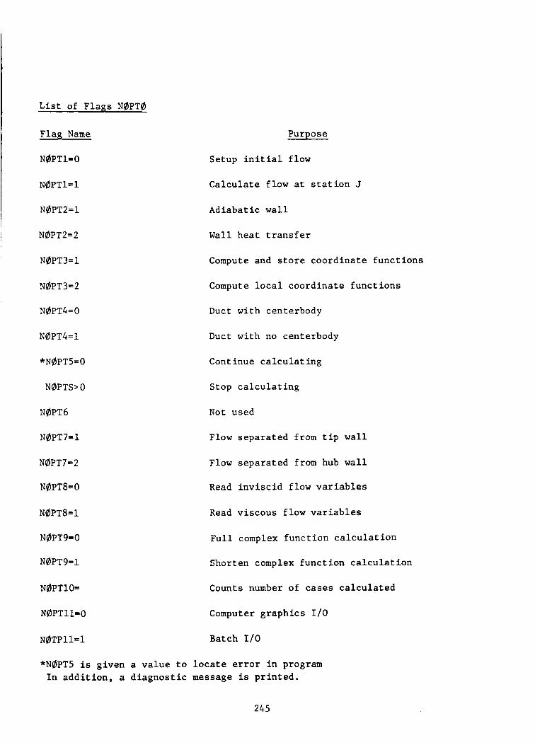
L i s t of F l ags N@PT@
Flag N a m e Purpose
N@PT 1= 0 Setup i n i t i a l f low
N@PT1=1 C a l c u l a t e flow a t s t a t i o n J
N@PT2=1 Ad iaba t i c w a l l
! N@PT2=2 Wall h e a t t r a n s f e r
N@PT3=1 Compute and s t o r e c o o r d i n a t e f u n c t i o n s
N@PT3=2 Compute l o c a l coord ina te f u n c t i o n s
N@PT4=O Duct w i th centerbody
N@PT4=1 Duct w i th no centerbody
*N@PT5= 0 Continue c a l c u l a t i n g
N@PTS> o Stop c a l c u l a t i n g
N@PT6 Not used
N@PT7=1 Flow s e p a r a t e d from t i p w a l l
N@PT7 =2 Flow sepa ra t ed from hub w a l l
N@PT8=O Read i n v i s c i d flow v a r i a b l e s
N@PT8=1 Read v i s c o u s f low v a r i a b l e s
N@PT9=O
N@PT9=1
F u l l complex f u n c t i o n c a l c u l a t i o n
Shorten complex f u n c t i o n c a l c u l a t i o n
N@PT10= Counts number of cases c a l c u l a t e d
N@PT11=0 Computer g r a p h i c s 1/0
~ 0 ~ ~ 1 1 - 1 Batch 1/0
*N@PT5 is g iven a v a l u e t o l o c a t e e r r o r i n program I n a d d i t i o n , a d i a g n o s t i c message is p r i n t e d .
245

N@PT13
N@PT14=3
NdPT14=1 I
N@TP15=O
N@PT15=1
N@PT16
N@PT17= 0
N@PT17 =1
N@PT18=O
N@PT 18= 1
?:@PT19= INFLl
N@PT20=O
N@PT20=1
N0PT2 1=0
N@PT2 1= 1
N@PT22=0
N@PT2 2=1
N@PT22=2
FCPLX f l a g
UN IVAC
I BM
I n t e g r a t e a long S t o o b t a i n s t r e a m l i n e
I n t e g r a t e a long n t o o b t a i n streamline
S t a t i o n coun te r
No b lade f o r c e c a l c u l a t i o n
Compute b l ade f o r c e
Turbulent f low
Laminar f low
NFLO i t e r a t i o n i n s u b r o u t i n e FLQWIN
Optimize KDS
F i x KDS
Greater than c r i t i c a l Reynolds number
Less than c r i t i c a l Reynolds number
S t a t o r
Rotor
P r o p e l l e r
246
APPENDIX A
Sample I n p u t Setups
I The i n p u t d a t a t o t h r e e sample c a s e s is shown i n t h i s s e c t i o n t o demonstrate how t h e i n p u t d a t a must b e s t r u c t u r e d i n o r d e r f o r t h e PANPER a n a l y s i s program t o o p e r a t e c o r r e c t l y . To i l l u s t r a t e t h e s e t u p of t h e d a t a i n p u t f o r c e r t a i n modes of o p e r a t i o n of t h e PILVPER program, t h r e e d i f f e r e n t s e t u p s a r e shown. The t h r e e s e t u p s are:
(1) I s o l a t e d P r o p e l l e r Configurat ion
(2) Combined Propel le r -Nace l le Conf igura t ion
( 3 ) Combined Coaxial Propel le r -Nace l le Conf igura t ion
The j o b c o n t r o l language (JCL) and t h e sample d a t a i n p u t f o r each of t h e s e config- u r a t i o n s are shown i n Tables ( I I ) , ( I I I ) , and ( I V ) , r e s p e c t i v e l y . The JCL commands are f o r a UNIVAC 1110 o p e r a t i n g system. e s s e n t i a l l y t h e same as t h e second c o n f i g u r a t i o n (Table 111) w i t h t h e a p p r o p r i a t e changes i n t h e mode c o n t r o l i n p u t and t h e removal of t h e p r o p e l l e r i n p u t d a t a .
An i s o l a t e d n a c e l l e c o n f i g u r a t i o n i s
24 7

m o m N r - Q P - N . . P I
P Q 4 N
. . n m
. . . . N Q N N - o 9 N . . . . 9 c O C .- 0 m N . . . . 0 tc P 0- 3030 J a n - .-. . .... n a o m C D Q P 3 c P m m P N r .... .... can- m a o m 9n*n -0." ....
In In c c
0 n 0 9 . m r N
N O N .
Q Q . N - 0
9 . 0 .
m n . O
0 . O S .Too
4 .
n n
. . f . . .- -N
.mo - a t . coo. QC em 0 0 0
3RIGINAL PAGE IS OF POOR QUALITY
0
N LL
a W
n 00 n
0
. . . . . - m n P m N r. - 9 0 P - f S . O 0 r m .
. . - . . ~n Q a - S . I n N . P 9
N 0 OQ N 0 -4) " . *In 9 . N* . e- 9 m - NN dd Q nn n. n -N 0 - m 00 e n
0 nt 9 1
. . . -- ... In- 0 09 O f 0 UlN 0 9- m- t m m m . . -4 0 1 - 00 .. n .... c -. ne 9 N Q S-I c.l mm OD . O C 90 . eo I n 0 c -e 0 . LO 00 . I . . . . . N - - fN . YIC I--
* I m I n - In
m m c e m c
e m C C . r ( . . - I n
0 ( * T y P I -I 0 . - 9 . . n * N
N - N d 4 . a n . N
9 - 0 .
# I N
. . n n . . . - 0 .
S O N t..
e n
.4-- .... norm C O N N Qc . - nP-" . .nn C m N N a m . - m n-4
....
n e
P O 9 . 0 . * 1
N U l N . 4 0 Q m - 9
a m 0 -
m a= . 0 0
0 dQ 0 - 1 fO . . f .e- .-09 - -ON no. . C P I n Q 9c4 I c)O - . . .O*
. .
. . m mr.
. . .
- m a c m c m . o n e s m Q . .
n r 0 . . 9 -
. 3 - 9
N - N .
o w 4 .
s o . - a . 0 - m a n e . r . . 0 . o m Y O - f .o ." .m
248

0000000 oooooao oooocoo o m a - ~ m m m m m - m m m O O O O O r n 0 0 0 0 0 0 0 .......
0 00 0 00 000
E m 0 000
mmm
.....
ORIGINAL PAGE IS OF POOR QUALITY
E W _ - _ ~ ~
nnn nnnnnvn
0 0 0 O R R R 0 R R C C L C L * * * . - ............... OGCOCOO
cocccoo m mmm mm m m o m m m m ~ 0000000 O P 0 0 0 0 R
oo=caaa
.......
" m 0
m 1 m . c e e r n . - . . D N
e 9 4 9
n r
e n . . N V ) N r - 9 a m . 9 . . o m n m d 0 .
m O f . PP . . . o -m 0 - 1 f a . -
. P I .-0 9
-ON na - CDmO 9 P I I ne I - . .D..l . .ma COCO I n - . . -nee NDa I ....
000 000 occ m m Q m m m 0 00
L
0 m n m m r - e e 0
e - n o 0 0 9 0
. . . .
. . . . N O N e
9 0 . . . . 9 N 0 -
I n 0
o m 0 9 N f000 f .e0 .4 .e
-90 - I-G-.n- 9c-00 n0-e .. .P
p m o - * m a * O n m e N*DD
n e . . - . .... .... .... ....
rn In e r-
0 m 0 9 m . f
N . N . d r n 9 9 . - . . . d
9 - O m
I n -
0 9 e - JON f . . .d .e . r m o
n O N d FP . . gc - - ne+= * .0- . e n -
t-m * * mm - - m n N * Ne-- . a n -
n m . . . .
....
In m I- r-
* 0 " 9 0 . o N - N *
9 0 . O
n
. . - 4
. . c " ? n . a - . v , . 0 e- o 0 0 f 0 .o f . . . ...la- . .-. nao- IC0 -0 Or- -0 - 0 9 . . .m-
m m I- P
; E n - D . 9 . . O . 9
N - N . - . 9 0 e m . - a . 0 .
m e . - . . n o
0 . o m f of- f .O ...l .m . . -0
nsoo eo*. 9-0 0 ne .O
. . I d .-e m m n m a * mnmm
m e I n N e m C N . . . . e - n e o m 9 N
N 9 N N - 0 Q N
9 - o r - I n N
. . . .
. . . . n o . . . . 0 I C 0 0- too0 f .mm
n 9 O m C R m D a - e m O P N I
r-mmc mmoy) m n e n NDNN .... ....
.4 .. ....
.... ....
m m P e
0
0 9
n
. m
. N
Z ? " - 9 0 . N - 0 9 . 0 . m n m n . O
0 - P J
J . .
. . fau -4 r N . .mo
- 0 3 . r-PO OI- .m no e o . .CN - .OO c m . . mm -. m n d - N O I N . .dO ....
In
r - 0 e * . 0
P . n a D * 9 0 . 0 . .
N O NUS a 9 o m . e 9 - 0 0
m m . P
0 -9 0 t-f f V N D
.Q0 . r e ....
m n
. .
. . n o . .
na .a a c m e ner-e
p m em I n m n n OnCIce N P O D
F D m f
. .e . ....
....
0 00 000 000 a m m mmm 000 e00 -..
0 0000 00 ouooaoa 00000c0 mmmmmmm mmmmmmm 0000000 e000e00
J
2 c3 Ll
ut; a .- 0
4 ....... - o n n n v n n n n m - moOoG0 mooa 03 cooooEjc .a mmm mmm mmmmmmm oooooc)o 0 0 0 0 PRO' .......
" OK. 9 0 0 3
J0 3 il .n 0 ON 0- J 0-
0 -
m
..
. . mI-
nnnnnnn
0 o?ooouo 0 00 ooc c 000 c nc p m ~ a m ) 9 m a w m x m m m a a00 GOO 0 0 0 P C D P ....... nnnnnnn
ND .N ..la
0
" c)
9 0
e o f D Y I c) . O 0 - 0 0
0 0 . - 0 I m . . 0 - 0 - n m e m n
D e m
24 9

a urn
o m * . O N - . . r . ,
ORiGlNAL PAGE i:; OF, POOR QUALiT'f
9 - . o c a C N - D O N . . . . . I
Q C . ~
m c m n - a D O " . . . - - I - * . e t * m o - m o r - - . O
m - l m o - 0 . 0 - 0 9
. o - 1 0 e - . n t - D N Y D
0 9 - . O N Y . . N n - - o f 9 " - . a - 9 . . 0 - m - 7 - e L n N f
. . .
g o m
. . .
ul m C e
i,
..I
O - O . . n . N
N e N - " . 9 - 7 . N
9 4 0 .
I n N
. . n n . . . " 0 . O n SUN f . . .-e- .... n ann CONN 9- . - mu.-- ....
m m Y I N
C N ~m . . . . V I n D
9 N e m . . . . N 9 N N - O 9 N . . . . 9 - G C
Y I N n o . . . . 0 .TI- 0 0- .TOO0 f .m" .- . . .... "IOOIII C D Q D
nDN- & - o m .... ..-. p m n c mm M nn-m
In m c C
0 m O 9 . m - N
N O N . m . a m . n ( . O
O . 0 . n n m n . O
0 - O f tOJ f .. . . -4 rN . rylo
Coo - 9- .ul
.CN
nat - ne -0 - .00 ca UlQ . - n n r - Ne-N . .ma ....
m m m N C Q C D . . . . D U n - e m a m . . . . N D N 9 I C
9 0 . . . . o m 0 - n e a n 0 . . . . 0 - O f S O 9
f .o .- .O
nand CPQ * 9Cr-- nDDQ .. .e *QQ &#'ION-
..,.
.... amr-m
I n 9 m a C D C e . . . - 0 l"
n 9 O D 9 0 . . . - N - N m - D O D . . . . a n O f W I D I n * . . . . 0 D f 0 NQ =OD* f .e0 .-. .. .... -9- f c o m a 9-P 0 n o o m .... .... W W C C W Q t m nno o
I n - m m c m C r ( . . 0 ,
~m n n O 9 9 - . . . . N N N P
a - . . . . 9 - 0 - m - m N . . . . 0 90 0 9 m t O f 0 t .N I ." . . .... n 9 N Q C D D W OCQO -7DNrl .... .... c m m m I n m o t 4n.T-
m m C C
0 n 0 9 f . n . N
N . N . - n 9 - . C J
4 - cu. LT. 4
. . n e . . . . O C
O Q 30- 3.. .4. . .n*
n9-J t-0 .N g c . . m o a . . .n1 - .Ch e m . . m m - . .onen ND'N .. .N .., .
m m C
e
P n 0 9 . O . .
N I N -
9 . . N
9 - o n m . m m
- c o r - e . t a m f . .
m "
. .
. - t m
'1ONC e@- I OC . . nOIno . -9c e m - I mm - - D R P -a
....
.... NO. - . .a9
m m C * D n * - I 9 0 . . . I
N O N N - 0 9 . . - . - O N 0 0 n . m - . N
0 0 O . 30- a..
. -
.dNN
- 9 . . eo-- 9 C . . mDNN . .OO . .e . - -00
m In C
C
. u l p -
n - D . a - . O . a
N - N .
* Q . * a . 0 - n o
I . . - m c . 4 . . 0 - o m f 0- *.a am . . -0 naoo eo9 . 9 C O - ne -0 . .I I .. .O c a m m a 9 - W n N m ND *N . .I 0 ....
: 9 ? n o r c a n s z z . O . . . .
NODO ..I. .... NO-- .... .... NDNN .... .... NDDD .... ....
N I - .
a N m
. O N o n t - . .
. . I 9 - . D C 9 C N - D O N
0 . 1 Q C . O r - m n - 9 D o - 0 . 1 - a - C I D m o - 0 0 - . . O
. . .
. . .
. . . " n
CI
0
m 1 I n . C f C t . O . . e -
m . O f 9 " I
. N
r y I n N -
" f 9 - . l n
. .
. . a m 0 . n m- In O f . I1.n
0 "0 0 - 1 f U - - f .e- .-am - .O0
"9 . C O f O 9-4 I ng -. . . fa . .9f cmr-m m m . m R C C NDC. I
. . .
.... . .D-
m c r I - 0 . e o 9 - 0 4
- 0 - 1 0 P I . n t
m In C C
0 n O - 9 . . I )
- N N - N - " . . D m . N
9 " n . m - l
. . n~ . . . " 0 . O n S O N
f . . .... n O"I-7 CDNN 9- . * no-- .... . ."In CDONN mm - nn-- N b . .
O N D
. 0 9 . . O
a o m
N-• N m - - O f 9 1 - . o - 9 . - 0 - Q n r - O N f . 0 -
. . .
. . . 0 . . D 4 N = o n
. o -
C 9 -
n n r .
t n t . . . n - .
O ~ N
. o . C . D U l Q D
N I 1 0 . O .
. . . m o m
250

ORIGINAL PAGE ES OF POOR QUALITY
Y) Y) c e . n
0 -1 n N
S ? . . . e
N N N O " . 9 . . e + N a n 0 0 n . I n . . m . u
0 ; . D O t u . 0 . . .rr - .m M s O N C D .U &I-. .
.CN . .90
n m m
e m 0 YIQ QDn .N NDSO . .r . . .- .
y l n e a Y ) N
e 0
D U n - 9 0
. . . . P O . . . . N D N Q - e 9 0 . . . . 4 m 0 -
- 0
D e D I J 090
0 .0 . n e . . . . .r .r .... nano 9-r-m noee
cmD1oo a n c m
CDQ"
.... .... m Q N a
ND0.D .... ....
m 9 I n 9 e 0 c 0
0 . N
0 . 0 9 0
. . . . n s . . . . N M I Y In
9 0 . . . . a n O I
m o
0 D J
;.UDD 0 .00
n e . . . . 0 r d a
.a .. .... nm-3 c D m 9 9CDD nD0D
c m c c Y ) Q 1 Y ) QnD0 NO.00
.... ....
.... ....
m a e m Y I Y )
+ I . . . . m u
e 9 9 -
n n
. . . . N N N e r m 9 - . . . . 9 - 0 - n r I n N
0 90. P a m t o n 0 .1 .Nd
. . . .
.- . . .... n 9 N Q c o o m 9CQ0 ne N-
cmmm m n i a
.... .... Y)Q 00
NDCl-4 .... .... Nlr-'*
Y) Y) e c
0 n 0 - 9 0 . . . r l
N - N N a 0 9 . . r l . .
O N 0 0
m - 4 - N
0 0
n . . .
-
a
0
0 c(
0 00 N J " 0
0
00 000QQQQQ Y)Y)Y)V)Y)Na*)NY) 00 ooooomo - - m m u w m n 00 O D D D D P D 0 . o o w o . . ... nn nnnnnnnn ...............
m a m m m m m m m m mmmmmomnNt 00 00000000 a - - r - N n n n m
nn nnnnnnnn 9,. 0 0 . D D D D D P 00000.. ... ............. 00 OOOOOOGO + f - c e f - D n a Y ) m D 00 00000000 oa ooooooc)o a- mma.mmmam oo wmmmmro mm 0000000000 eo 0 0 0 0 0 0 0 0
nn nnnnnnnn ..........
~
0 0 0
0 -
.......... 00000. . ... - nn nnnnnnnn ...............
............... nnnnnnnmmn oooouuoouo 00 uo OOU uo 0 00 GUCOO Do0 ~ a m m a m m m D 1 o r o mm 9 I u ~ Q Q ~ ~ u ) onoonnoooo 0 0 0 0 0 0 0 0 0 0
00 -N 00
00 0 9 0 0 0
000 ... ............... s;.
nnnnnnnnnn n*
... . . . _ 00000000. . ... .O 9
25 1

APPENDIX B
Example of PANPER Analys is Programoutput
The purpose of t h i s appendix i s t o g i v e an example of t h e p r i n t o u t The c a s e t h a t is ou tpu t from t h e PANFER a n a l y s i s program f o r t h e case ,
which i s used t o demonstrate t h i s p r i n t o u t i s t h e a n a l y s i s of a n a c e l l e - p r o p e l l e r c o n f i g u r a t i o n (Table 111) . This type of c o n f i g u r a t i o n w a s used as a tes t c a s e i n r e f e r e n o e 1. The e n t i r e p r i n t o u t from t h i s sample c a s e w i l l n o t be inc luded i n t h i s appendix b u t r a t h e r s p e c i f i c areas of t h e p r i n t o u t are l i s t e d i n o r d e r t o i l l u s t r a t e t h e ou tpu t of t h e v a r i o u s t a s k s t h a t t h e program performs. P r i n t o u t w i l l be shown f o r t h e fo l lowing t a s k s :
(1) Main Program Heading and Output of I n i t i a l P r o p e l l e r Inpu t Data
( 2 ) O u t p u t ' o f t h e Options and Inpu t D a t a used i n Nacelle Analys is
(3) Output of t h e Nacelle Geometry
(4) Output of t h e I n v i s c i d Flow S o l u t i o n (At Axial S t a t i o n ZH = .76489)
(5) Output of t h e L i f t i n g L ine Noninduced In f low Condi t ions
(6) Output of t h e Options and Reference Data used i n P r o p e l l e r Ana lys i s
(7) Output of S e l e c t e d I n t e r m e d i a t e C a l c u l a t i o n R e s u l t s f o r t h e P r o p e l l e r An a 1 y s i s
(8) Output of t h e P r o p e l l e r Performance R e s u l t s
(9) Output of t h e P r o p e l l e r Blade Forces
(10) Output of t h e N a c e l l e V i s c o u s Flow S o l u t i o n ( A t Axial S t a t i o n ZH = .76489)
25 2

0 0 0 0 0 0 0 0
+ 0 + 0 0 0 0 + + 0 0 + 0
0 0 0 0
+ + + 0 0 0 + + + 0 0
0
: f + a 0 - * o 0 0 + a + a
0 0 0 0
0
+ I 0 i
i 0 + 0
I
0 I 0 ' , ' 0
0 + 0 0
i
I
I i 0 0
I 0 0 + + 0 + 0 + + 0
(.
I i
!
I m 0 + 0 0 0 0
0 + 0 0 + + 0
+ 0 + + 0
+ + 0 + + 0 0
+ + + 0 + 0 + + + 0 0 + + + + + + +
+ 0
0 + * + 0
0 0 0
+ + + +
+ 0 a
N a m
I- X w 0 0 0 t I a n t I 4
N a - a a W
0 9
7
A
a W 0 e z f
e u W 7 0 a a
m - Z
U 1 a c H
b 0) I4 r( QI a 0 & PI d m +I U +I C H
* u J u o u t - + z z + - w + a + T U
R W c z W U + o x
O L U
0 w
W A OQ
ZUO - u oo a
0 0 0 + 0 + 0
+ 0 + + + + + + 0 + 0 0 0
0
0 0 0 0 + 0 + 0 0
., 0
+ + 0 + 0 + + 0
0
0 0 0 0
0 0 0 0 0
e 0 0 + 0
&I 0 U 1 0. c1 1 0 Q c m
2 d Q m 01 z
s b M 0 b
PI
z c Ih 1 - a z u a 4 a w n 0 a P I
I
I !
I I
I !
a w a w CI
0
X - W
a
a
1 : c d m 2:
a W c a
I O , x I Z
I y I @ d - . . 1 0 r N a O a m ; r t - . ooocooo 00000 * * * * * * I * I * * *
O O O O O J a o o 0 0 0 0 7 3 0 3 0 0 0 J J C oosooaocaooocoaoaooooo; ~ 0 3 0 0 0 3 3 0 0 3 0 0 0 ~ 0 3 0 0 ~ ~ ~ c ooocoo~oooooa30oaoono-c 3 o ~ Q a ~ h o o o o u o a a a 3 0 3 a ~ - u ~ 0 0 o 0 0 J 0 0 0 0 m 0 S O O C 0 0 h ~ a a ~ r ~ a r a ~ O . . I ~ w N ~ O 0 0 0 0 0 ~ O r C
oocc **.I
0 0 C G O O O O O O O O O O ~ C O C 0 0 t Q C
. e . . . . . . . , . . . * . . . * . . . . . I I
n I4 W
I
1 ' !
i i I
25 3

10 1 0
0 0 0 0 * ' 0 0
0 , 0
0
0 0 e 0
O N 0 .o
c(
0 I c) U II) (Y
a
O d 0 0 * I o a e *
0 0 m o a - n n D N
c In
N n
* I
0 0 a o n d
a a n
0 ; ; O , N * e * !
I o m 0 0
' I 0 0 d o C O r n ~ a N . .
0 0 0 0 * * 0 0 - 9 ' c - V I 0 a m . .
0 0
01
C m Q
c)
. 0 - 0 0 0 0 * I * 0 4 -
e - t I - m N O d d , . . .
I 0 - a 0 0 0 * I I 0 9 9 o d n e ~ c n n o - O - m . . .
I
0" 0 0 ; 0 0 ' 0 0 0 0 0 0 0 0 0 0 * * * * * * * * 0 0 0 0 ' 0 0 0 0 I n 0 m o r , o V I - V I - V I - I n - V I N c n e a C m C Q I - - C O C - I - N . . . e . . p .
I
o - - 0 0 * I 0 0 I n 0 m o C Y ) C N
0 0 0 0 * *
0 0
0 Y) d I- IC
0 3 m n V I 0 C O I - O . .
O N 0 - 0 0 0 0 a o a o 0 0 0 0 * * * * * * * * 0 0 0 0 0 0 0 0
0 0 0 0 O - 253 n f i n o n e
0 - a 0 * I 0 0 e o n u
0 0 a 0 * *
C 3
0 0 n O 9
O N - F ? ?
0 0 0 -
O Q 9 0
n m . . - e n e > 0 9 o m 9 N 9 N 9 - . . Q N . . . . b .
O Q O N . .
O N 0 0 * * 0 0 N O N e - n Q N . .
0 0 0 0 * * 0 0 N O N m - m 0 -
0 - 0 0 * I a 0 N O N O a n a n . .
a 0 J C + * N u l C V Q - 9 0 . r
o a
. . i
(3
2 3 N Y
f d
0 0 0 0 * * 0.3 N Q r y N
4 N . . . . O N 0 4 0 0 0 0 0 0 0 0 . o a a o 0 0 0 3 Q S
7 3 , * * * * * * O O 9 0 . O O O I - 0 - o m . O D O I -
ca r.
5 ? ?
. . P O o m a b b o c o c o 0 0 0 0 0 0 O t c o C P - e a 0 0 o u 0 0 O N Z Y a n s - 8 Y V I z o = u t~ 3 1 - t n t f t ~ . . . * . . . . . * . . .
- a * Q f f . . .
C t I-
C.
c ?-.
n m N m Q . 9 . . . 0 - - 0 0 0 * I 1 '0 - N O N Q n n -
0 0 n o r r d
0 0 ,
I- 0 ' a m n -
n o
. . 0 0 n c I - m Q O n N . .
o c * 0 n o n o
n a
r - u 9 0 . ' .
I
a n n N . . 9 0
u l f - . .
254

n
0 0 + 0 0 0. 0 0.
0 0 0 0 + + 0 0 a i 0 m 0 n 4 0 4 . e
d 0 + 0
0 0
1
4 . 1
0
0 c1 0 0 r(
r(
3
3 4 0 0 4
r(
0 a J 0
a
4 . 1
0 + CI 0 0 C 4
s 0 + 0 C. a 7. s
0 3
c 0 3. 3.
a
C 8s + 9 - 0 T a.
0 0 + 0 In m 0. 0.
0 0
P) m 0. 9.
a
0 0 0 0 + + 3 0 V I 0 m m r - f r - 4 . .
0 a
0 0 3 5 * *
- . . c o 3 0 * * 0 0 N O N O u e . D - " .
- - 0 3 0 * +
c - n a- n 0 >
r- n a 0 c i 7.1 . .
I 1
0 a
25 5
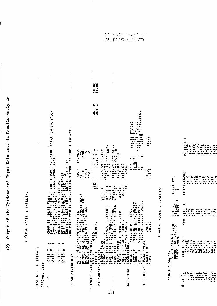
cn .rl cn h d
? aJ rl rl aJ V m z C .r(
Q a cn 3 a U m &a u 3 a C H
a C m 2 0 d 4 4 a 0 01
5 cec 0 U 3 a U 3 0
n N W
AI z c(
-I W m 4. rn d
d w c 0 .: z 4 LL a
n .O %
n W v) 3
w l 2 0 m C
0 n
z 0 c(
C a A
U -I * u w U
0 LL
w
e d 5a z ou LC
w No I Z &O -1V * -I
zu
a
a
n
a0
o-I
ul c 2 c(
0 Q
I- 7 0 z c1
CI 0- I I W - IX
C -0 - LQ: x - I L L
CeC re-
000 300 nap ;Lon c(*u m u m
I
9 In .n .. .U-OVIN c r
O f 0 LLLL O r N 90 *? a- 4 30
00 .. 1 1 I1 I 1 ~
I I I I
I 1 I 1
SI- mv) no
L-
uc 3U 03 0
v)
ezza a noon o u-*.d w
W W 0
00 00
0 0 . 9 . N
I 1
W l l 53 de sa ua
at3 09
f 0 a- ..
r * u c 0 2 I A U 4 L L X a. a
e o I Y L L
I v ) & a W t u S m n
i
25 6
W U z W K w LL W a
4 U 2
-1 Y
a m a 3 b
3 vmln 5 2- 3 Q
0 I U
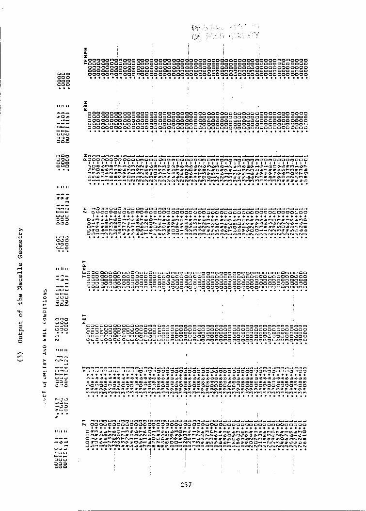
t a E
~ 0 0 0 0 0 0 0 0 O O P 00000000 000O00000O0000000OO000000000000 O00OOOQOOOO 0 0 0 0 0 0 0 0 0 0 0 0 0 0 0 0 0 0 0 0 0 0 0 0 0 ~ Q 0 0 0 0 0 0 0 ~ 0 0 ..................................................
W 0 0 0 0 0 0 0 0 0 0 0 000000000000000000000000000 000000000000
000 00000000 o~oooooo aoooo ooooooooooaooo oooao 000 0000 aoaaa 00aaoo 0000 ooaooooo ooooo0oooo0ooooaoooooo~0o
I
t m X oaooooao 0ooo0oa~ooo~0ooooooa0oa~0ooooooaooo~0ooooo 000 00000 000000 00 000000 000 34 oaaaoo JO ooo ooo 00 ooo 0000 000 00000 000000 00 000aOO 000 00 ~ 0 0 0 0 ~ ao m o o a00 GO 000 000 0 000 00000 000000 00 000000000 3Q 00000~ 00 000 a 00 e0 000 000 0 0 OC 000 Pg OcOOaO 00 0000 0 0 0 0 ~ 00 oooaoa oooooooo oo oC0 0000 ..................................................
c m
.................................................. c N
C 0 c 0 L3 .
!
25 7
, I
!
woaaoooooooooooooooaooooow aooooo 00 aooaooooaw o w aoooaaaooaooaoaaoow oooooaw oooooo moaoomooooooao m o o oa oooaoa ooa ooooa aaooaoao aaa oaa 00 oooooa oao oo ooa moo oa ooaoaoooooooao oooooaoa ooooaa aaoooooaoaoao ooo 3 oo o oa oo ao aa oao o ao oo ao o aoa 00 ooa oao 00 000 0 00 Oa 0 00 00 0 ..................................................
oooaaaoaooaoaaoOOooaoaaoooaaoao awoaoooaoaoooooow oaooouoo.~oaooooaooaaooao~oooo~~ aoaoaoao aaoooo3oooo oooaoaoaaooooooaooaaooooaoaooao aoacaooo ooooooooooa doc ooooaoaoo aoo oaoao aoo oo aoaaoo ooaooo oo ooa oo o oaa 00 coo oaaooo oooaao oooaaoao oa oooooo oooooo cg ooo oaoooooa ..................................................
!
roaooooooOOoooooooaooaoooaoooaoo~ooooooaooooooa~ oooo~oooooooc~oooo 3oaoaaaoooo ooo ooo oo ooo o w oooaoooo l * * * * * * * + * * * * * * * * * * * ~ * * * * * * * + * * * * * + * * * * * * * * + + + * * * *
................................................... 0. L?
- aoac ooccOoccooocoac~ooaooooo ~aocaoocoooooococccoouc c ...................................................A 9
c c a 4 2 w 30
a a
W r c(
I-
258
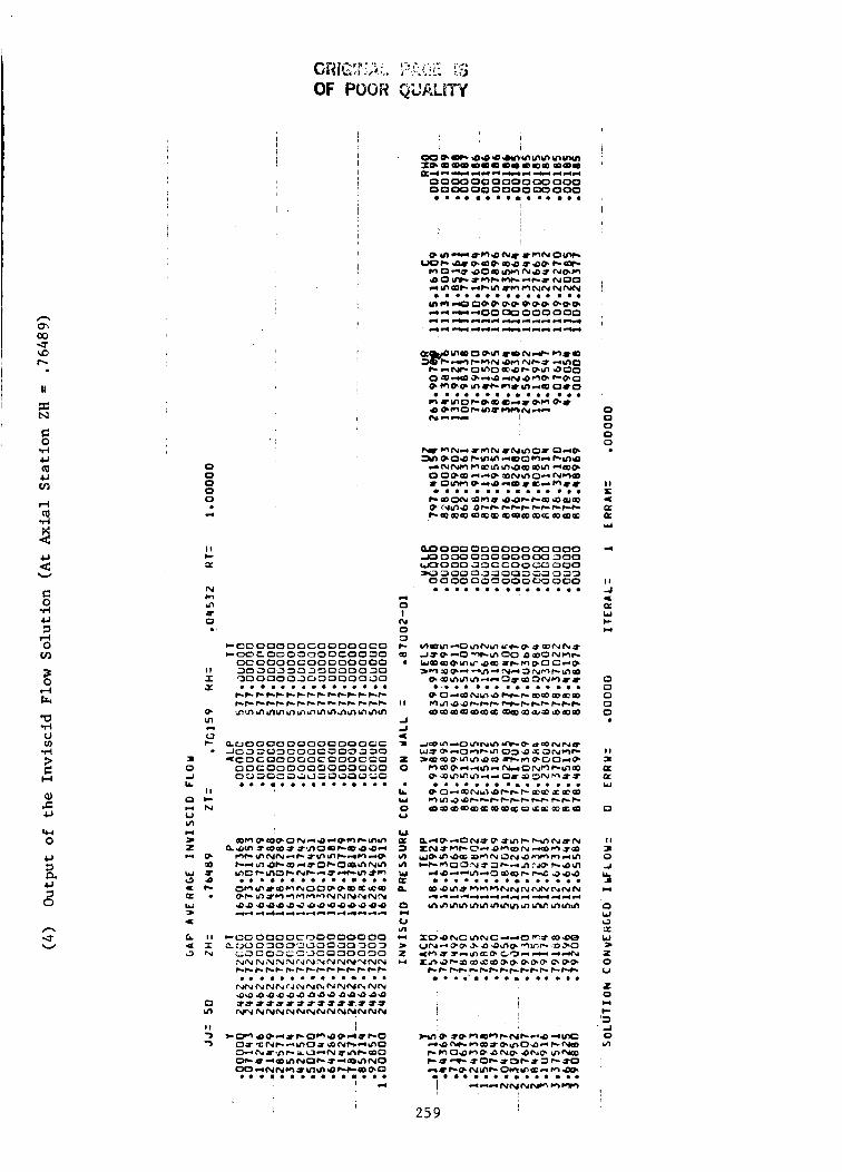
u v 4
g d U 7 rl 0 cn
ad x d 3 C H
01 5 cer 0 U 7 a
2
0 0 0 0 0 . 4
I 1 c X
N n a t 0 ..
I1 I 5
0. m CI
0 C
I 0 2 L
I1 a c n N u VI CI w 2 n 0
W t a 0 a + I L . W w
a
L I I a s O N
0 m I 1 3 -J
I
I
cocaoooocoooooco coocoooaaoocoo3o ccoooocoooooooo aoao3a33goaoa3o '30 000 0 20 3 0000 30
ccooooocnoaaoooo P 00 0 30 OCU a 0 a0 3 0 3 LO ooa= s'~G039010 CVrY N N N N r.( rY N N NcY Y NN CI-I-r-CC+C*+r-++f-I- ............... N N C V N N F J N N P U N N N N " Q Q O 9 9 9 9 9 9 9 0 9 9 0 ~ f f t t t f f f t f f t t t f W W W Y N N N N N N W N N N N
CI
0 I N 0 3 I- Q . I I
2 A U I
2 0
k w 0 V
W
3 vl ul Y
0
Q n u ul I W
b4
a
a
2
I
uo 00 00 0 000 00 000 oopo 000000 00 000 ...............
I
I 1 i
MOOOOOOOOOOOOOO &aox)o1oooooo7oo WOO00 J 1 C C O O O C O O O w 3 Q o 3 5 3 o ~ a a a ~ 5 3 0 0 00 030000 000 ...............
i i
I 25 9
I
I
I
0 0 0 0 0 . I I E U
a ul
a
- I I 2
a W c I
a 0 0 0 0 . I 1 = a a w
0
I 1 I. 0 -I I& J c(
0 W 0 1: W W z 0 u 2 0 cI( c d 0 v)
la
1

I rn
I d rec H C
U 3 a u 3 0
COC O O Q O O O O O ~ r r zoo ~ O O O O O O C oa
260

I ! !
. N
I 1 cn w W a W I 1. 3
LL 0
L. 2 0 z -
! - -
0 0 0 0 0 .
. 0 2
I I Z 0 U .
0 la W a W
a I 1
c LL
a u
VI
w a
0 0 .
A A W
0 a a n z w W
c a
m d I1 L-
A a V
2 I: LL:
7 2 W
d d 0) a 0
a u 2
N
Y) m m
. 0 W 0
c(
b m N a
c(
0 0
W m c 5 U S a4 U a A vl U 3
a
0 r( e
rl . a QI v) 3
I t
> c m v) Z w 0
I I w w U c 3 U
e
a U a Gl n a
-1 0 0
A 4 m X 4
QI W a o -1
4 m c m 2 m
W
0 a W da 0 -3
I-0 ..
r- vl w
0 0
0 a. f m
r(
0 W 2 A W
0 (t
a
a CY 0 Y-
dl U m c vl c i: W c U 4 2 Q
U
f L d -1 L' a. 3
A.
-
* c a 0
a 8 - c
A 9 I Am v u.
x a 0 Lux L Y e a0 ac m 02 -0 >W a
2 . I: oa 0 ow Luo u o z w e m
vl
LL
m c)
0 N
a c a z -4 0 1: 0 0
v) 9 d I c IL
(to -0 I- o
0 d d
L
>U I * n
.. vl
w e a
l l .. 9
m 6 I:
a W E * I I
vl
I I d 3 3 iL 0 c
o c v l v l
U
o w c
o i ) u a W P
-I V
a L U c a W
- 0
z w x - 1
-1 - u m o * e 0 N Z V I 0
L 'L
I t 0 w v
n e
a a
o a c
( v a
m a
a * 0
4
a n U
3 a U 3 0
9 2 n c 6 2 w 0 a
-1 n h 0
5 2 I
0 L
vl z 0 U
n \o v
I l l
L O H c
> z c .J s. 0
c a 0
a z I A W 0 0
. x a W a a
d
a a U 1 1 a h i I I
VI
w d -1
a a Q L
c( 0 E a U
W la
W 30 oa -IC L X
x.
P a ul
a n
n 2 a
1 V U
!i ? 8
c LLZ O b W
0
0-
n a
W a a
dr u r 00 u
.G za
d m
A- m>
26 1

U e U n 2 U
c .. CI
M
-. W c 3
x 0 u 0 c W x c(
c
a
2 W
0 0
a
a , a 0 LL
e 3 c
0
X * 0 0
P
a a
a
a
m W I I- C( c z * 3 U * c W L a w a
a
W a a m LL 0
c u . 4 . . . - ....... 5 I I l l - ,
26 2
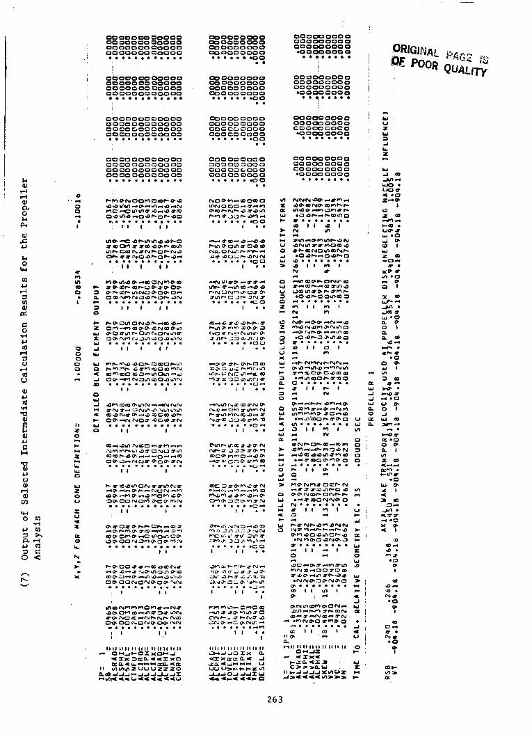
!
i
I
I I
d
a w d A W
0 a
000000000000 000000000000 00 00000 00000 0000000 00000 ............
000000000 DDooooooo 00 000 0 00 0 000000000 .< 0 . . e 0 0 .. 4 ) O O D O 0 0 0 0 0000 00 0 00 0 00 0000
995 93 ss:: 8 .. 00 000 000 0 00 000000 0
.O 0 Qo 000 0 ........ oo o oo ooa o
oooooooao O O O r n 000 0 coaoo aoco
S O 0 00 000 0 . . a * . . * .
000000000 00000 0000 COOOQOOOO -0omoaoo ........
000000000000 0000000 00000 000000000000 000000000000 . a; a <
I
0000000 00000 0000 000 00000 oacc toaooa 00
?3999?9??945
0000 000000M) oa oo aoa a ao oo 00 oo ooa a oa oo oa oo oooaoo ao ............
c. L u ’ u z w 3 d LL 2 U
~ 0 0 0 0 0 0 0 ooooooaoo O O G C G ~ ~ U ~
43 9 c.? 7% 8 .. 000 00 000 0 301003000 ooo co tca a acoooaaao ... ...a0 ..
0 I ’ r(
0 0
I
*
t m ul 0
a a l
0 D 0 0 0
d
I 1 z 0 n c n 2 U LL w 0
w I: 0 V
r V < I
0 LL N
* X
a
- .
b 0 rw rn 4J rl
2 a p:
W P a d m a W a n < c W 0 w
a * c c(
U 0 d w >
0 0 3 ’ 0
?
a rl a VI
W o w
...... .J- I I I ..
I
26 3

W u z a X K 0 k.
W a a K W d a W
0 a K a
3 0
CI 1 2
Q n w 0 4 a a
a w d d W a 0 a a d
f 0 Y c Y wl 0 a K 2 0 a
2 6 4
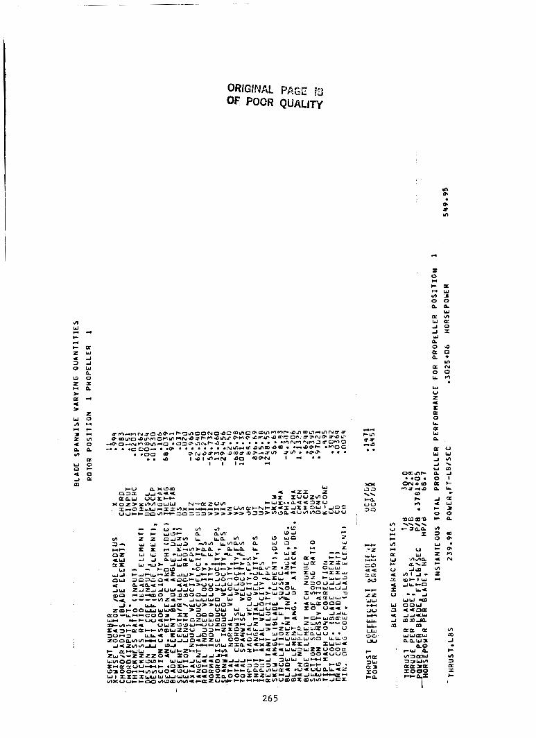
ORIGINAL PAGE IS OF POOR QUALlw
2 0 m C K m w ul 0 0 a n
w a m w a d o d 1 ul a 0 9 P O a . 4
ul O N 0 0 L r )
W V z e
a 0 L
W
r
a a a u w w

ORIGINAL PAGE IS OF POOR QUALITY
c w L-J d > a
2
WW W Z W A A
_ - e voz
U d v) .
9. t 2
V
I W A J W
0
a. 0 W c a 0 W c 2 m
a a
a
d ‘2 < a LA
c m 2 3
a a W
W 5 U
)m a a W
W u a 0 .L I
I
2 W CI z
.. E - r I3 0 a a A .( e 0 c
W c W
< c
a
a w A A W
0 a a a
a I ir c LL Q W
A U w 0 a a
a W c 3
L: 0 V
0 c
W x n +
a a t 0 V
0 c
W r I 1111 I I 1 1 1 1 I I 1 1 1 1 1111111 uwrv)mv,VIvlv)VImVI aaa aa aaa aa,a
I I
n r
266

- ooa r l I I t m N 3 -.13u-l
... I I
u) aJ 0 LI 0 cr a Q a rl c9 LI a
0) a 0
JJ 3 0
n Q\ v
............ 1 1 1 1
26 7

d
rcT . *mdr(dr( Y r(der(---md-t"NN& NN"NN(W"N Nhnr WNWN .03000 00 000 00000000 OOOOO 000 aooooooo 00000000
b l l ! 1 I I I I I I I I I I I I I t I I f 1 I I I 1 I I I I 1 1 I 1 I I 1 1 I 1 I 1 I I t
n m a0 \D I-
ll
X N
C 0 .r( . . U a U
d F4 v) 1 0 c) v) d 5
, l-l d aJ 0 a z
u 0 U 3 a U 7 0
I
PAGE IS QUALITY
w 0 a
I i I !
.............................................. I m
................... *. .............
Gc. 70
00 c'30 00 000000000 Ot OOOPOOOOOOO OOC M O O O O O G GO UOC .. * * e * * * * * * * * * * * * * * * * * * * * * * * * * * * e * * * * * * * * * * * * * e 3oc 30 0 0 S 3 0 C 3 0 003 30 300000 00000 000 00 000 034 coo00
co 33

ORIGINAL PAGE Is" OF POOR QUALITY
Fl 0
I I
c a
1 0 3
. . - 0 . . ........................................ W
a 0 1
?- a 3 *7 N
I 1 n a
c

APPENDIX C
L i s t of Symbols
a
A
A+
- - A
=k A
B
=k B
C
‘fr
C P
P
v
DFr
C
C
Dpr
ens
Ens
e
f
F
t r ans fo rma t ion v a r i a b l e
A r e a , a/r2 (d imens ionless )
Van Driest c o n s t a n t (26.0)
Schwar tz -Chr is tof fe l parameters
Block t r i d i a g o n a l ma t r ix (d imens ionless )
Diagonal b lock m a t r i x (d imens ionless )
chord , b / r r (d imens ionless )
L e f t d i agona l b lock m a t r i x (d imens ionless )
Speed of sound ( f t / s e c )
Wall f r i c t i o n drag c o e f f i c i e n t
S p e c i f i c hea t p r e s s u r e ( f t 2 / s e c 2 / d e g R)
P r e s s u r e d rag c o e f f i c i e n t
S p e c i f i c h e a t volume ( f t 2 / s e c 2 / d e g R)
F r i c t i o n d rag
P r e s s u r e d rag
Streamwise s t r a i n ( l / s e c )
Streamwise s t r a i n , r e
Tangen t i a l s t r a i n ( l /sec)
Tangen t i a l s t r a i n , r ren+/ur (d imens ionless )
fo rce / span
Complex p o t e n t i a l ( s + i n ) , body f o r c e
r
/ur (d imens ionless ) r n s
2 70

gB
G
h
I
m
M
M
0 m
m+
n
NB
R N
P
PrT
Q
a r
R
CR
S
Gap between b l ades ( f t )
Gap between b l ades , g g / r r (dimensionless)
Duct he igh t
Entropy
Mass f low ( s l u g s / s e c )
Mass f low, m/(FJBr2p r r r U ) (dimensionless)
Mach number, U/C (dimensionless)
Mass f low/a rea ( s l u g s / f t 2 / s e c )
0 * Universa l mass f low parameter , mJ(pWu ) (d imens ionless )
Mass f low/area, g/(PrUr) (d imens ionless )
Normal coord ina te (d imens ionless )
Numb er of b l a d e s ( d imen s i o n l es s)
Reynolds number , r r p r U r / p r (dimensionless)
Pressure (lb/ f t 2,
To ta l p r e s s u r e
Turbulent P r a n d t l number
Heat f l u x , q/(prUrCpTr) (dimensionless)
H e a t f l u x
Rad ia l coord ina te
Radius , r/rr (dimensionless)
Gas cons t an t ( f t2 / sec2 /deg R)
Streamwise coord ina te ( dimens ionless )
271

S t r e a m w i s e coord ina te , s / ( r rVr) ( d h e n s ion1 e s s )
S
S t a n t on numb er ( d imen s i o n l es s ) S t
Temperature (deg R) T
T o t a l temperature TO
U Nagnitude of v e l o c i t y o r v e l o c i t y component
Tangen t i a l v e l o c i t y u@ U+ Universa l v e l o c i t y , U/U* (dimensionless)
F r i c t i o n v e l o c i t y , &/Ur (d imens ionless ) U*
P o t e n t i a l f l o w v e l o c i t y ( 1 / ~ m e t r i c scale c o e f f i c i e n t )
V
Complex coord ina te s i n d u c t p l a n (r + i z )
W
Dis tance a long S and n c o o r d i n a t e s
Yt Universa l d i s t a n c e
Axial c o o r d i n a t e Z
Axial d i s t a n c e , z / r r (dimensionless) 2
a S w i r l a n g l e t o a x i s (deg)
R a t i o of s p e c i f i c h e a t s , Cp/Cv ( d imen s i o n l es s )
Y
Boundary l a y e r t h i c k n e s s , b / r r (dimens i o n l e s s)
A
A* Displacement t h i c k n e s s , 6*/rr (dimensionless)
N o m 1 c o o r d i n a t e , n/(rrVr) (d imens ionless ) , o r Transformed normal c o o r d i n a t e (dimens i o n l e s s )
rl
272

I
K
x
51
n
P
P
c n s
c n@
T T ns , n9
T+
X
Angle of s t r e a m l i n e t o axis (deg)
Temperature r a t i o , T/Tr (dimensionless)
Momentum t h i c k n e s s , O*/Tr (d imens ionless )
J -1 Entropy, ( I - In) / R (dimensionless)
von Karman cons t an t (0.41)
Thermal conduc t iv i ty ( lb / sec /deg R)
V i s c o s i t y ( s l u g s / f t / s e c )
3.14159
P r e s s u r e r a t i o , p/pr (dinlensionless)
Densi ty ( s l u g s / f t 3 )
Densi ty r a t i o , p / p r (d imens ionless )
Streamwise stress, T,,/(P,U,) (dimensionless)
Tangen t i a l stress, Tn@/(prUr) (d imens ionless )
2
2
Stress components
S t r e s s , T / T ~ (d imens ionless )
Tangen t i a l coo rd ina te ( r a d i a n s )
Blade d i s s i p a t i o n f u n c t i o n
Clauser cons t an t (0.016) (dimensionless) , o r Transformation f u n c t i o n , d d d n (d imens ionless )
Stream func t ion (d imensionl ess)
2 73

Matrix Opera tors
T
-I
S u p e r s c r i p t s
V
Subsc r ip t s
0
1
2
3
A
E
H
I
n
r
Transpose
I n v e r s e
I t e r a t i o n number
Mean o r average q u a n t i t y
Var i ab le s f o r b l ade f o r c e c a l c u l a t i o n
Devia t ion from mean q u a n t i t y
S tagna t ion c o n d i t i o n s
I n l e t c o n d i t i o n s
Upstream of s t r u t b lade
Downstream of s t r u t b l ade
Ad iaba t i c
E f f e c t i v e t u r b u l e n t
Hub cond i t ions
Incompress ib le c o n d i t i o n s , s i n g u l a r i t y index
i n t h e d i r e c t i o n of t h e normal
Reference c o n d i t i o n s , based on s t an - dard sea l e v e l atmosphere c o n d i t i o n s f o r a l l thermodynamic q u a n t i t i e s . The r e f e r e n c e r a d i u s rr i s t h e i n l e t o u t e r r a d i u s , and t h e v e l o c i t y i s t h e mean i n l e t v e l o c i t y
2 74

S u b s c r i p t s (Cont'd)
S
T
W
m
i n t h e streamwise d i r e c t i o n
Tip c o n d i t i o n s
Wall c o n d i t i o n s
F r e e Stream o r edge of boundary l a y e r
2 75

REFERENCES
1.
2.
3.
4.
5 .
6.
7.
8.
9.
10.
11.
Egolf, T. A., 0. L. Anderson, D. E. Edwards, and A. J. Landgrebe: Analy- sis for High Speed Propeller-Nacelle Aerodynamic Performance Prediction. Volume I: Theory and Initial Application. *
Landgrebe, A. J . : The Wake Geometry of a Hovering Helicopter Rotor and Its Influence on Rotor Performance. Journal of the American Helicopter Society, Vol. 17, No. 4, October 1972. (Also preprint No. 620, 28th Annual National Forum of the American Helicopter Society, May 1972.)
Coles, D. E.: The Law of the Wake in the Turbulent Boundary Layer. J . Fluid Mech., Vol. 1, pp. 161-260 (1956).
Wislicenus, G. F.: Fluid Mechanics of Turbomachinery. McGraw-Hill Book Co., Inc., 1947.
Black, D. M.: Cascade Corrections to Isolated Airfoil Data. Internal Correspondence, Hamilton Standard, ~ ~ 1 4 0 1 , October 8, 1974.
Anderson, 0. L.: User's Manual for a Finite-Difference Calculation of Turbulent Swirling Compressible Flow in Axisymmetric Ducts with Struts and Slot Cooled WallstUSAAMRDL-TR-74-50, May 1974.
Van Driest, E. R.: On Turbulence Flow Near a Wall. Journal of Aeronau- tical Sciences, Vol. 23, November 1956.
McDonald, H., and R. W. Fish: Practical Calculations of Transitional Boundary Layers. International Journal of Heat and Mass Transfer, Vol. 16, No. 9, pp. 1729-1744, 1973.
IMSL Library 2 Reference Manual, Edition 6 C. International Mathematical and Statistical Libraries, Inc., 1977.
Schlicting, H.: Boundary Layer Theory. 6th Edn. McGraw-Hill, New York (1968).
Mellor, G. L.: A Combined Theoretical and Empirical Method of Axial Compressor Cascade Prediction. Report No. 9, Contract N00019-69-C-0520, Naval Air Systems Command, May 1970.
* I Date and NASA Contractor Report number to be filled in later.
I 2 76
REFERENCES (Cont'd.)
12. Bielawa, R. L.: Aeroelastic Analysis f o r Helicopter Rotor Blades with Time-Variable, Nonlinear Structural Twist and Multiple Structural Redundancy - Mathematical Derivation and User's Manual, NASA CR-2638, October 1976.
13. Johnson, J. A. and R. 0. Bullock: Aerodynamic Design of Axial Flow Compressors. NASA SP 36, 1965.
2 7 7

ORIGMAL PAGE IS OF POOR QUALln
Q INPUT
COORDINATES
INECLECTINC PROPELLERSI
INECL~CTING PROP€ LLERI
PERTURBATIONS DUE TO NACELLE
BLADE FORCES
C A L C U U T E VISCOUS FLOYV F IELD FLOW F IELD NACELLE DRAG
t
Figure 1. Flow Diagram of the Combined Propeller-Nacelle Analysis
278 85-4-90-20

9 A
x. P I T C H A X I S \ \ u " v
Figure 2. Cylindrical and Cartesian Coordinate Systems for Propeller Geometry
279 86-4-90-21

GENERA Ll ZED DISTORTED WAKE
\ c-
TOP VIEW
VIEW
CLASSICAL WAKE
Figure 3. Computer Wake Representation for One Blade of a Hovering Rotor, Classical and Generalized Distorted Wake Models
280

\ " O C
r m a x
Figure 4. Modeling the Wake Rollup with Discrete Vortices
28 1 86-4-00-23

r n
0 2 a a m
N a
> 0 W
-I
TIP VORTEX RADIAL COORDINATE
O-
RW I 1 r
TIP VORTEX AXIAL COORDINATE
K 0 AXIAL COORDINATE OF VORTEX SHEET EXTENSION TO r = 1
s o 5 2 zw
W Y
X
Q z a
a 3 n- -1
AXIAL COORDINATE OF VORTEX SHEET EXTENSION TO r = 0 Q
4
Z W - A K l 0 . -
zw I +AK20’(PHI--”) 0 1 t AKZO-IPHINPO-812) 2 a I + AK30. (PHI-PHINPO)
? I I
n :I 0 12 I1 - I
-1 z 12 2 , -
WAKE AZIMUTH, PHI (CONVERTED TO RADIANS)
Figure 5. Generalized Wake Geometry Equations Containing Input Wake Constants
28 2 85-4-90-24

21 - TWT , AMWT
J
IOPT3 = 1 STRAIGHT ANNULAR DUCT
ANGT
R T l
I f -
IOPT3 = 3 STRAIGHT WALL ANNULAR DIFFUSER
I-- .[ f
r R T = R T l + (RTL-RTl)'SINfPI'Z/Z1 I" A T
RH = RH1 + (RHL-RHI). SINIPI'ZIZ1)"AH
IOPT3 = 5 CURVED WALL DIFFUSER NO. 1
Figure 6. Preprogrammed Duct Wall Contours
283 81-4-90-25

DST
a : a I-
AMSl
DH = ( l+ANH) DSH
Y = O / /
DSH
Figure 7. Inlet FLOW Distribution
284 85-4-90-26

INNER WALL
Figure 8. Addition of Straight Annular Channel Inlet
285

Figure 9. Discontinuous Change in Wall Curvature
286 86-4-00-28

STRUT
'////
7 / / / / / /,,/ 1
I
EXTENDED DUCT
z
Figure 10. Extended Duct Section
28 7 85-4-90-28

PT c I bT
Y
Figure 11. Constructing the Inlet Flow
288 85-4-00-30

START
f IWK = 1, NPROP
- (PROPELLER
WAKE)
J
INTERMEDIATE CA LCU LATIONS
i
(GENERALIZED) (INPUT WAKE GEOMETRY 1
(C LASS1 C A L, MODIFIED
CLASSICAL)
COORDINATE c.-i PRWZW
(PRINT WAKE COORDINATES)
IP = 1, NPROP
DISK)
(PROP E L LE R
LL = 1, LTOT (PROPELLER
POSIT I ON)
I
CALCGC (COMPUTE INFLUENCE
COEFFICIENTS)
WRITGC (WRITE
COEFFICIENTS TO DISC)
IWKrNPROP
RETURN
8 6 4 - 9 6 3 1
c3 Figure 12. Flow Diagram of Subroutine GCWAKE
28 9

START c2 PHICAL
(COMPUTE AZIMUTH POSITIONS)
A
INT IAL ( INITIALIZE INPUT DATA)
PER F 0 RM AN C E ITER AT1 ON VALUES)
NO
1
PERFOR (CALCULATE PROPELLER
PERFORMANCE)
GCWAKE (CALCULATE WAKE GEOMETRY 81 GEOMETRIC COEFFICIENTS)
CTITER (CALCULATE THRUST
PERFORMANCE ITERATION VALUES)
NO -
b
B LDG EO I v
SOLVIT
k
VECTOR (CALCULATE VELOCITIES)
I (CALCULATE AERODYNAMICS SOLUTION) I
I I
ci RETURN
Figure 13. Flow Diagram of Subroutine PROP
290 85-4-80-32

START
t REDMAT
(READ MATRIX)
CALCULATE LINEARIZED
AERODY NAMl C QUANTITIES
A
0- CORRECT10
I 1
MCONE
(EVAARD TYPE RELIEF)
Figure 14. Flow Diagram of Subroutine SOLVEL 8b--CBO-33
291

START 0
VVECTR
(CALCULATE VELOCITY
RELATED QUANTITIES)
REDMAT (READ MATRIX)
YES v
MCONE (EVAARD TYPE RELIEF)
CALCULATE NONLINEAR
AERODYNAMIC QUANTITIES
0 RETURN
Figure 15. Flow Diagram of Subroutine SOLVEN 292
85-4-90-34

ALTMN
INITIALIZE PROGRAM
READ MODE SWITCH
RETURN Q PERFORM
ANALYSIS
5-1 * READINPUT C PROPELLER
<
2.0 SET UP PROBLEM
CONSTRUCT DUCT AND
NORMALIZE
COMPUTE EX ACT
COORDINATES
COMPUTE INLET FLOW
APPROXIMATE COORDINATES
I
I
W R IT€ OUTPUT
t
CALCULATE
>
I
Figure 16. Flow Chart for ALTMN
293
COR RE CTl ONS
CALCULATE
FORCES
85-4-90-35
4.2 SOLVE VISCOUS FLOW -
PROBLEM

M > 1 M < 1
I I I I
c- REVERSE FLOW
"1
Figure 17. Iteration Procedure
xo 1.0
294 86-4-90-36

COORST (=?
-
I I 1.0 INITIALIZE VARIABLES
MSLOT<_ NSLOT - - 8.0 INSERT N E X T SLOT
2.0 F I N D UPSTREAM AND DOWNSTREAM SLOT LOCATIONS
- RETURN -
SOLVE FOR
CHRISTOFFLE TRANSFORM
SCHWARTZ -
' MSLOT>NSLOT
9.0 COMPUTE DUCT WALLS -f- WITH SLOTS
2.5 INTEGRATE I N STR E AMWl SE
DIRECTION
6.0 STOR E COORDINATES
-
Figure 18. Flow Chart for Subroutine COORST
295
85-4-90-37
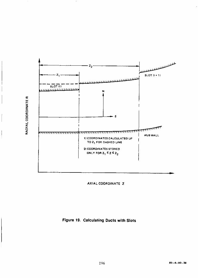
SLOT ( I )
I
I
7 I f f 1 1 1 1 f 1 1 f f f f ~ f ~ f ~ J f J ~
1 ) COORDINATES CALCULATED UP I TO Z1 FOR DASHED LINE
I
I 2) COORDINATES STORED
ONLY FOR 2 , Z s Z2
L
AXIAL COORDINATE 2
Figure 19. Calculating Ducts with Slots
296 85-&BO-38

START (7
t 1 ' NORMALIZE
INLET FLOW DATA
*
I
- -
PO = Pr < 0.001 r TO = Tr
t.o.001 I
RADIAL EOUlLlBRlUM FOR ISENTROPIC
FREE STREAM FLOW
CALCULATE INLET
FREE STREAM
FLOW FROM M i , a1 T
1
I
INTERPOLATE
I
CALCULATE
IN LET FLOW
CALCULATE
BOUNDARY LAYER L
FROM 6.. n. TW
I I -
CALCULATE m, ur,
M AND NORMALIZE
c3 RETURN
Figure 20. Flow Chart for Subroutine Flowin
29 7 85-4-90-39

START v YES I R T = 0
T H I CK NESS
(LINEAR (POLYNOMIAL INTERPOLATION) F I T )
I I 1
DEFINE GAP, SOLD, ZLE, ZTE
o - 0 LROW = 1
LROW =
A
Z L E L = ZLE ZTE L = ZTE CALL BLDlN
N O
t No I .
Z L E L = ZLE ZTE L = ZTE
IRT= 1 CALL BLDlN
Figure 21. Flow Chart for GBlade
298 85-4-90-40

START a
NORMALIZE
INPUT ARRAYS
c 0.001 SET INNER
SURFACE CONTROL
BOUNDARY
- - -
DUCT ARRAYS
I
-
CALCULATE
- - STRAIGHT
PARAMETERS WALL DUCT
=1 -
I
L
= 2 - READ DUCT - = 2 - READ DUCT -
CALCULATE
WALL ANNULAR - - STRAIGHT
= 3 - - -.I
PARAMETERS DIFFUSER
‘I > 3 f
CALCULATE
WALL ANNULAR DIFFUSER
= 4 - NACA CURVED -
> i 0.001
0 RETURN
Figure 22. Flow Chart for Subroutine GDuct
299 06-4-00-41

Figure 23. Locating Lifting Line in Steamline Coordinates
300 85-4- 90-42

SET INlTlA CON DlTlOh
NOPTl - 0
I
- >zz SAVE RJ NOPT1 = 0 JKDS = JKDS + 1
4
l-I-/ COORDINATES _- . . . N Z T
I 1
1
COMPUTE INITIAL c STRESS AND
HEAT FLUX
= O -
- - UPDATE - - d COMPUTE SOLVE MATRIX
SOLUTION FOR DEPENDENT VARIABLES
COMPUTE MEAN FLOW WRITE SOLUTION -
AT JJ STATION APPLY CORRECTIONS
RETURN
E-4399 Figure 24. Flow Diagram for Subroutine SOLVl
30 1

1. Report No. 2. Government Accession No.
NASA CR-4199
4. Title and Subtitle
An Analysis for High Speed Propeller-Nacelle Aerodynamic November 1988 Performance Prediction
Volume 11-User’s Manual
3. Recipient’s Catalog No.
5. Report Date
9. Performing Organization Name and Address
United Technologies Research Center Silver Lane East Hartford, Connecticut 06108
12. Sponsoring Agency Name and Address
T. Alan Egolf, Olof L. Anderson, David E. Edwards, and Anton J. Landgrebe
535-03-01
11. Contract or Grant No.
and NAS3-22257
Contractor Report
NAS3-20961, NAS3-22142,
13. Type of Report and Period Covered
None (E-4399)
10. Work Unit No.
’ 17. Key Words (Suggested by Author@))
~ Computer code High speed propeller Aerodynamic performance Propfan
18. Distribution Statement
Unclassified - Unlimited Subject Category 02
15. Supplementary Notes
19. Security Classif. (of this report) 20. Security Classif. (of this page)
Unclassified Unclassified I I
Project Managers, Lawrence J. Bober and Christopher E. Hughes, Propulsion Systems Division, NASA Lewis Research Center.
21. No of pages 22. Price’
308 A14
16. Abstract
A user’s manual for the computer program developed for the prediction of propeller-nacelle performance reported in “An Analysis for High Speed Propeller-Nacelle Aerodynamic Performance Prediction. Volume I-Theory and Application” is presented. The manual describes the computer program mode of operation requirements, input structure, input data requirements and the program output. In addition, it provides the user with documentation of the internal program structure and software used in the computer program as it relates to the theory presented in Volume I. Sample input data setups are provided along with selected printout of the program output for one of the sample setups.
“For sale by the National Technical Information Service, Springfield, Virginia 221 61 NASA FORM 1626 OCT 86
a u . s . GOVERNMENT PRINTING OFFICE: 1 9 8 9 - - 6 ~ 7 - 7 8 5 - - 8 0 0 a o