projections of global changes in precipitation

GEOPHYSICAL RESEARCH LETTERS, VOL. ???, XXXX, DOI:10.1029/,

Projections of global changes in precipitation1

extremes from CMIP5 models2

Andrea Toreti,1 Philippe Naveau,2 Matteo Zampieri,3 Anne Schindler,1

Enrico Scoccimarro,3,4 Elena Xoplaki,1 Henk A. Dijkstra,5 Silvio Gualdi3,4,

and Jurg Luterbacher1

Corresponding author: A. Toreti, Dept of Geography, Climatology, Climate Dynam-

ics and Climate Change, Justus-Liebig University of Giessen, 35390 Giessen, Germany.

([email protected])

1Dept. of Geography, Climatology,

D R A F T September 2, 2013, 3:28pm D R A F T

X - 2 TORETI ET AL.: PRECIPITATION EXTREMES

Precipitation extremes are expected to increase in a warming climate, thus3

it is essential to characterise their potential future changes. Here we evalu-4

ate eight high-resolution Global Climate Model simulations in the twenti-5

eth century and provide new evidence on projected global precipitation ex-6

tremes for the 21st century. A significant intensification of daily extremes for7

all seasons is projected for the mid and high latitudes of both hemispheres8

at the end of the present century. This signal supports a dynamical influence9

of the polar warming amplification on precipitation extremes.For the sub-10

tropics and tropics, the lack of reliable and consistent estimations found for11

Climate Dynamics and Climate Change,

Justus-Liebig University of Giessen,

Giessen, Germany.

2Laboratoire des Sciences du Climat et de

l’Environnement, IPSL-CNRS,

Gif-sur-Yvette, France.

3Centro Euro-Mediterraneo sui

Cambiamenti Climatici, Lecce, Italy

4Istituto Nazionale di Geofisica e

Vulcanologia, Bologna, Italy.

5Dept. of Physics and Astronomy, Utrecht

University, Utrecht, The Netherlands.


TORETI ET AL.: PRECIPITATION EXTREMES X - 3

both the historical and future simulations might be connected with model12

deficiencies in the representation of organised convective systems. Low inter-13

model variability and good agreement with high-resolution regional obser-14

vations are found for the twentieth century winter over the Northern Hemi-15

sphere mid and high latitudes.16



1. Introduction

Exposure and vulnerability to weather and climate-related natural hazards largely de-17

termine the severity of impacts of these extremes [IPCC , 2012]. In the context of climate18

change, where considerable changes in the frequency and intensity of extremes are ex-19

pected, the development of adequate risk-reduction strategies and measures is crucial.20

Since planning requires reliable knowledge of the relevant climate phenomena, a robust21

characterisation in terms of frequency and intensity of current and future extreme precip-22

itation is of great relevance. Changes in mean annual precipitation have been observed in23

different regions of the world, with decreasing tendencies over the tropics and subtropics24

of the Northern Hemisphere (NH), increases over the northern mid and high latitudes25

and over the tropics and subtropics of the Southern Hemisphere (SH) [Trenberth et al.,26

2007; Zhang et al., 2007; Trenberth, 2011]. A widespread increase both in the frequency27

and intensity of daily precipitation extremes has already been identified [Alexander et al.,28

2006; Min et al., 2011; Westra et al., 2013], although uncertainties arising from the lack of29

observations at the daily scale and the interpolation procedures applied for the production30

of available gridded data sets affect the estimations of precipitation extremes [Trenberth31

et al., 2007; Chen and Knutson, 2008; Hofstra et al., 2009; O’Gorman and Schneider ,32

2009; Min et al., 2011; Trenberth, 2011]. In the NH, this upward tendency (that has been33

identified in the second half of the twentieth century) has been linked to human-induced34

greenhouse gases increase [Min et al., 2011]. Global Climate Models (GCMs) still cannot35

adequately capture the frequency, the intensity, the tendency and the spatial distribution36

of observed precipitation extremes over large regions in the world [Sun et al., 2006; Allan37



and Soden, 2008; O’Gorman and Schneider , 2009; Min et al., 2011].38

Global warming implies an increase of atmospheric water vapour content at a rate of39

about 7%/K, through the Clausius-Clapeyron equation [Allan and Soden, 2008]. Hence,40

a comparable increase in extreme precipitation would be expected over the next decades41

[O’Gorman and Schneider , 2009; Kharin et al., 2013]. A significant reduction in return42

times of annual extremes of daily precipitation (20-year return level) has been globally43

projected for different radiative forcing scenarios for the late 21st century with large inter-44

model disagreement in the tropics [Kharin et al., 2013].45

Here, we evaluate the simulated daily precipitation extremes in the 20th century assum-46

ing stationary processes [e.g., Scoccimarro et al., 2013]. This implies that the ability of47

the models to reproduce the observed tendencies in specific regions of the world is not48

considered. Furthermore, we provide for the first time a comprehensive global assessment49

of seasonal future changes in daily precipitation extremes identifying regions where both50

consistency (i.e., models agreement) and reliability (i.e., goodness-of-fit of the applied51

statistical model) are achieved.52

2. Data and Methods

Simulations for the period 1966-2099 were retrieved from the Coupled Model Intercom-53

parison Project CMIP5 [Taylor et al., 2012]. Eight models with a horizontal atmospheric54

resolution higher than 1.5◦ were chosen (Table S1) and daily precipitation data were re-55

trieved. As for the projections (2006-2099), the high emissions scenario RCP8.5 and the56

mid-range mitigation emissions scenario RCP4.5 [Moss et al., 2010] were selected. With57

respect to observations, an equivalent global high-resolution daily precipitation data set58



covering the historical period 1966-2005 does not exist. Therefore, freely available high59

resolution regional products were retrieved. As shown in the Table S2, these gridded60

products have a spatial resolution of 0.25◦ and 0.05◦ over Australia. They do not cover61

the entire world, but they provide a very good coverage of the Euro-Mediterranean re-62

gion, Northern Eurasia, the Middle East, Asia, Australia and North America. Concerning63

Northern Eurasia and the Middle East, the two associated gridded data sets have a limited64

overlapping with the Euro-Mediterranean data set. Further details as well as maps of the65

covered regions can be found in the associated publications [Higgins et al., 2000; Jones66

et al., 2009; Haylock et al., 2008; Yatagai et al., 2012] and the related web-sites (Table67

S2).68

Since the eight GCMs have different resolutions and grids, and precipitation is highly de-69

pendent on the spatial scale, all daily gridded values were remapped onto a common grid70

with the coarsest resolution of 1.5◦ by applying a conservative remapping procedure [Chen71

and Knutson, 2008]. By applying the same procedure, in order to allow for a comparison72

between gridded observations and model simulations for the historical period 1966-2005,73

observations were remapped to the common grid of the models.74

As for the characterisation of the extremes and their changes in the 21th century, we com-75

pare the two 40-year time periods 2020-2059 and 2060-2099 with the historical period. The76

length of the two periods ensures an adequate data amount for the statistical inference77

that is known to be data-demanding for extremes. In order to assess the goodness-of-fit78

of the statistical model (hereafter, reliability), stationary processes within each 40-year79

period were assumed.80



The analysis was performed in the frame of Extreme Value Theory by applying a Peaks81

Over Threshold approach [Davison and Smith, 1990]. In this context, the distribution of82

excesses over a high threshold (here, set as the 90th percentile) can be modelled by using83

the Generalised Pareto (GP) family, i.e.84

Hσ,ξ(y) = 1− {1 + (ξy/σ)}−1/ξ, ξ �= 085

Hσ,ξ(y) = 1− exp(−y/σ), ξ = 0 (1)86

where σ > 0, y ≥ 0 when ξ ≥ 0 and y ∈ [0,−σ/ξ] when ξ < 0. The two parameters σ and87

ξ are called scale and shape parameter, respectively. As soon as an estimation for both88

parameters is available (ξ and σ), the return level zR (i.e., the value that is expected to89

be exceeded on average once every R years, here 50) can be estimated by:90

zR = u+ σξ−1

�(Rζu)

ξ − 1�

(2)91

where u is the chosen threshold and ζu is the intensity of the Poisson process which is92

assumed to describe the occurrence of the excesses. Concerning the parameters estima-93

tion and in order to avoid numerical problems connected with optimisation procedures,94

we applied the Generalised Probability Weighted Moments method (GPWM, see the Ap-95

pendix) [Diebolt et al., 2007].96

The goodness-of-fit of the estimation was tested by a modified Anderson-Darling statistic97

[Luceno, 2006, and references therein], i.e.,98

A = n

� ∞

−∞[H(y)− Fn(y)]

2 · [1−H(y)]−1dy (3)99

where n denotes the number of excesses, H is the assumed theoretical distribution (here,100

Generalised Pareto) and Fn is the empirical distribution function. Since the parameters101



of the distribution H were not known, the asymptotic distribution of A and, thus, the102

critical values (at the 0.95 level) for the test were also unknown. As a consequence of ap-103

plying the GPWM method, the covariance of the Gaussian process to which the integrand104

of A asymptotically converges cannot be approximated. Thus, the critical values for the105

test were obtained by using a bootstrap procedure [Babu and Rao, 2004].106

In brief for the bootstrap procedure, let y1, . . . , yn be the excesses and σ and ξ the esti-107

mated parameters. Then, m additional samples (in this exercise, 1000) can be generated108

from Hσ,ξ and the A statistic can be computed m times by estimating the shape and the109

scale from the generated m samples. The critical values for the test can be derived from110

the calculated m values of A.111

In order to perform an inter-model comparison with respect to observations in the his-112

torical period 1966-2005, Taylor diagrams were used for the estimated return level fields113

[Taylor , 2001].114

3. Results

Changes in precipitation extremes are presented in terms of very high risk events, i.e.,115

50-year return levels (values that are expected to be exceeded on average once every 50116

years) derived by the inferred distributions.117

In the historical period, as shown in Figure 1, a reliable characterisation of daily extreme118

precipitation cannot be achieved for larger areas of the world, where an estimation of119

the return levels cannot be obtained. This is the case during boreal winter for a belt120

elongated over the subtropics and tropics of the NH and the oceanic areas west of the121

three continents of the SH. In boreal summer, unreliable estimations (i.e., failing the122



goodness-of-fit test) are found mainly over the eastern North Pacific, north-eastern Africa123

and Arabian Peninsula as well as a large part of the Mediterranean basin and the east-124

ern North Atlantic, eastern South Pacific and north-central Australia. A similar spatial125

pattern is also identified for spring and autumn (not shown). Lack of reliability roughly126

corresponds to areas characterised by higher positive values of the shape parameter (not127

shown) and therefore strongly heavy-tailed Generalised Pareto distributions. Although128

spatial differences do exist, this correspondence is a common feature of seven out of eight129

models and could be connected with the parameterisation of convection in regions receiv-130

ing smaller amounts of seasonal precipitation [Dai , 2006], poorly represented land- and131

ocean-atmosphere interactions as well as deficiencies in the representation (position and132

shape) of the Intertropical Convergence Zone [Huang et al., 2004; Dai , 2006; Richter and133

Xie, 2008; Good et al., 2009].134

For the mid and high latitudes, six out of eight models show a spatially homogeneous tail135

behaviour with slightly negative and positive values of the shape parameter (not shown).136

This means that the probability of precipitation extremes either has a finite upper bound137

or decreases approximately exponentially or slightly slower towards zero. Nevertheless,138

a glance at the individual simulations reveals remarkable inter-model differences as well139

as areas with a larger probability of higher extremes. In the Euro-Mediterranean area,140

northern Eurasia and North America, the simulations show lower inter-model variability141

and higher correlation with the observations in boreal winter (Figs. 1 and S1). Conversely,142

for Australia, southern Asia and the Middle-East all seasons are characterised by larger143

inter-model variability and lower correlation with the observations (Figs. S1-S2).144



For the period 2020-2059, both scenarios reveal reliable and consistent changes only for145

scattered areas in the mid and high latitudes of both hemispheres (Figs. 2 and S3). A146

similar global pattern with regional differences is estimated for the other seasons (not147

shown). It is worth noting that the intensity reduction over the northern tropical Atlantic148

is strongly seasonally dependent as it almost disappears in boreal summer and is less149

pronounced in spring and autumn.150

Towards the end of the 21st century (2060-2099), a similar pattern but with more pro-151

nounced changes compared to the middle of the century is projected under the RCP8.5152

scenario. For the RCP4.5 scenario, for which the radiative forcing stabilises in the second153

half of the 21st century, changes in extremes are less pronounced. Consistent and reliable154

increases of precipitation extremes are obtained for all seasons over the mid and high lati-155

tudes of both hemispheres mainly for the RCP8.5 scenario. In the SH, the spatial pattern156

of consistent and reliable areas does not show a marked seasonal dependence. In the NH157

within the zone showing consistency and reliability, different areas can be highlighted for158

each season (potentially connected with sea ice changes [e.g. Budikova, 2009; Screen et al.,159

2013]), for instance Northern Eurasia in boreal winter; the North Pacific, the northwest-160

ern Atlantic/Arctic Ocean in boreal summer (Fig. 2). Meridional differences are clearer161

in the zonal means (Figs. 3 and S4). They show more pronounced increases over the162

high-latitudes of both hemispheres in all seasons, with the exception of the NH in the163

mid-century boreal summer, associated with larger inter-model variability. Over the SH,164

a sharp decrease in the estimated positive changes from the high to the mid latitudes is165

evident in all seasons and, with the exception of the austral winter, followed by a strong166



increase towards the low latitudes. Over the NH, the poleward meridional increase of the167

estimated positive changes is almost continuous in boreal winter (Fig. 3) and autumn168

(not shown), while a stepwise poleward increase is projected for summer (Fig. 3) and169

spring (not shown). Stronger hemispheric differences (Fig. 3) are estimated over the high170

latitudes for RCP8.5 at the second half of the century that are most prominent in sum-171

mer (11% difference between the NH and SH spatial means) and autumn (15% difference172

between the NH and SH spatial means). The largestLargest changes at the second half of173

the century are found over the high latitudes of the NH for autumn (45%) and for spring174

in the SH (39%). For the mid latitudes in the same period, mean regional changes are175

highest in the NH autumn (37%) and the SH summer (30%). No reliable assessment can176

be made for the subtropical-tropical regions (Fig. 3). The identified increase of extremes177

for the 21st century (although seasonally and regionally dependent) is higher than previ-178

ously estimated for annual extremes [Kharin et al., 2013]. The effect of stabilisation of the179

radiative forcing in the RCP4.5 scenario is evident in Figure S4, showing less pronounced180

differences between the two periods 2020-2059 and 2060-2099 compared to the RCP8.5181

scenario.182

In order to gain a better insight into the regional changes, twenty six land areas [IPCC ,183

2012] were selected and the inter-model variability of the regional means is provided in184

the Figure 4 and Figs. S5-7. Remarkable seasonal and regional differences are evident185

among the twenty six land-areas. Reliable extremes characterisation can be made for186

62% (65%) of the land-areas in boreal winter (summer) and for 88% (85%) of the areas187

in spring (autumn). For some areas, reliability shows a clear seasonal dependency (e.g.,188



southern Europe), while this is not the case for regions such as Northern Europe and189

Northern Asia. Finally, it is evident from the results that the regional averages show a190

better agreement between models.191

192

4. Discussion

In the tropics, the identified lack of reliability and consistency in extreme precipitation193

could be associated with a deficiency in the representation of upward velocities that seems194

to introduce large differences in climate models output, an underestimation of the response195

to global warming [Allan and Soden, 2008; O’Gorman and Schneider , 2009] as well as196

with model difficulties in reproducing processes based on organised convective systems197

[Zhang , 2005; Benedict and Randall , 2007]. Conversely in the mid and high latitudes,198

where large-scale processes play an important role [O’Gorman and Schneider , 2009], re-199

liable and consistent results are coherent with the increase of precipitation extremes not200

only constrained byare coherent with the Clausius-Clapeyron constraint equation but also201

dynamically driven and potentially connected withand could be dynamically linked to the202

polar warming amplification [Schlosser et al., 2010; Jaiser et al., 2012; Francis and Vavrus ,203

2012; Screen and Simmonds , 2013], although this connection needs to be investigated and204

is our next research issue.205

At the regional level, models show a better agreement on the projected increase of return206

levels over land, although large variability affects the estimated seasonal changes over207

specific areas (e.g., Eastern Asia in summer). Finally, it is worth to point that for some208

areas such as the Indian Monsoon region, where models deficiencies were also identified209



by Hasson et al. [2013] and Sperber et al. [2013], reliable estimations cannot be achieved.210

211

Appendix A: the GPWM method

The GPWM for the Generalised Pareto distribution are defined by212

µω = E {Y ω (1−Hσ,ξ(Y ))} (A1)213

where E denotes the expected value and ω is a continuous function null (and with right214

derivative) at 0. An estimator of µω is given by [Diebolt et al., 2007]:215

µω,n =� ∞

0W (1− Fn(x)) dx (A2)216

where n represents the number of excesses, Fn denotes the empirical distribution function217

of the excesses and W is the primitive of ω. For applications (as in the current exercise)218

a good choice for the function ω is ω(x) = xr with r = 1, 1.5. This implies that µω = µr219

can be estimated by:220

µr = n−1

n�

i=1

Y(i) ·�(n− i)n−1

�r(A3)221

where Y(i) represents the ordered sample of the excesses. Finally, the estimated parameters222

are provided by using the following equalities, replacing µ1 and µ1.5 with their estimates:223

σ = (2.5µ1.5µ1) · (2µ1 − 2.5µ1.5)−1 (A4)224

ξ =�4µ1 − (2.5)2µ1.5]

�· (2µ1 − 2.5µ1.5)

−1 (A5)225

This approach is valid for ξ ∈ (−1, 1.5).226

227



Acknowledgments. A.T., J.L., E.X. and P.N. acknowledge support from the EU-FP7228

ACQWA project (n. 212250). A.T. acknowledges DFG (grant TO829/1-1). We thank F.229

Albrecht for computational support and P. Fraschetti for data retrieving and computa-230

tional support. We acknowledge the World Climate Research Programmes Working Group231

on Coupled Modelling for model simulations. We thank EU-FP6 project ENSEMBLES,232

NOAA/OAR/ERL PSD, Aphrodite’s project and the Bureau of Meteorology Australia233

for gridded observations. We thank two anonymous reviewers for their comments and234

suggestions.235

References

Alexander, L. V., et al., Global observed changes in daily climate extremes of temperature236

and precipitation J. Geophys. Res., 111, D05109.237

Allan, R. P., and B. J. Soden (2008), Atmospheric Warming and the Amplification of238

Precipitation Extremes, Science, 321, 1481–1484.239

Babu, G. J., and C. R Rao (2004), Goodness-of-fit tests when parameters are estimated,240

Sankhya, 66, 63–74.241

Benedict, J. J., and D. A. (2007), Randall Observed characteristics of the MJO relative242

to maximum rainfall, J. Atmos. Sci., 64, 2332–2354.243

Budikova, D. (2009), Role of Arctic sea ice in global atmospheric circulation: A review,244

Global Planet. Change, 68, 149–163.245

Chen, C. T., and T. Knutson (2008), On the Verification and Comparison of Extreme246

Rainfall Indices from Climate Models, J. Climate, 21, 1605–1621.247



Dai, A., (2006), Precipitation characteristics in eighteen coupled climate models, J. Cli-248

mate, 19, 4605–4630.249

Davison, A. C., and R. L. Smith (1990), Models for exceedances over high thresholds, J.250

Roy. Stat. Soc. B Met., 52, 393–442.251

Diebolt, J., A. Guillou, and I. Rached (2007), Approximation of the distribution of excesses252

through a generalized probability-weighted moments method, J. Stat. Plan. Infer., 137,253

841–857.254

Francis, J. A., and S. J. Vavrus (2012), Evidence linking Arctic amplification to extreme255

weather in mid-latitudes, Geophys. Res. Lett., 39, L06801.256

Good, P., J. A. Lowe, and D. P. Rowell (2009), Understanding uncertainty in future257

projections for the tropical Atlantic: relationships with the unforced climate, Clim.258

Dyn., 32, 205–218.259

Haylock, M. R., et al. (2008), A European daily high-resolution gridded dataset of surface260

temperature and precipitation, J. Geophys. Res., 113, D20119.261

Hasson, S., V. Lucarini, and S. Pascale (2013), Hydrological cycle over south and southeast262

Asian river basins as simulated by PCMDI/CMIP3 experiment, Earth. Sys. Dynam.263

Discuss., 4, 109–177.264

Higgins, R. W., et al. (2000), Improved United States precipitation quality control system265

and analysis, NCEP/Climate Prediction Center Atlas.266

Hofstra, N., et al. (2009), Testing E-OBS European high-resolution gridded dataset of267

daily precipitation and surface temperature, J. Geophys. Res., 114, D21101.268



Huang, B., P. S. Schopf, and J. Shukla (2004), Intrinsic ocean-atmosphere variability of269

the tropical atlantic ocean, J. Climate, 17, 2058–2077.270

IPCC (2012), Managing the Risks of Extreme Events and Disasters to Advance Climate271

Change Adaptation. A Special Report of Working Groups I and II of the Intergovern-272

mental Panel on Climate Change, C. B. Field et al. Eds, Cambridge University Press,273

New York.274

Jaiser, R., et al. (2012), Impact of sea ice cover changes on the Northern Hemisphere275

atmospheric winter circulation, Tellus A, 64, 11595.276

Jones, D. A., W. Wang, and R. Fawcett (2009), High-quality spatial climate data-sets for277

Australia, Aust. Meteorol. Ocean. J., 58, 233–248.278

Kharin, V. V., et al. (2013), Changes in temperature and precipitation extremes in the279

CMIP5 ensemble, Climatic Change, doi 10.1007/s10584-013-0705-8.280

Luceno, A., (2006), Fitting the generalized Pareto distribution to data using maximum281

goodness-of-fit estimators, Comput. Stat. Data An., 51, 904–917.282

Min, S. K., et al. (2011), Human contribution to more-intense precipitation extremes,283

Nature, 470, 378–381.284

Moss, R. H., et al. (2010), The next generation of scenarios for climate change research285

and assessment, Nature, 463, 747–756.286

O’Gorman, P. A., and T. Schneider (2009), The physical basis for increases in precipitation287

extremes in simulations of 21st-century climate change, Proc. Nat. Acad. Sci. U.S.A.,288

106, 14773–14777.289



Richter, I., and S. P. Xie (2008), On the origin of equatorial Atlantic biases in coupled290

general circulation models, Clim. Dyn., 31, 587–598.291

Screen, J. A., and I. Simmonds (2013), Exploring links between Arctic amplification and292

mid-latitude weather, Geophys. Res. Lett., 40,959–964.293

Screen, J. A., et al. (2013), Atmospheric impacts of Arctic sea-ice loss, 19792009: separat-294

ing forced change from atmospheric internal variability, Clim. Dyn., doi:10.1007/s00382-295

013-1830-9.296

Schlosser, E., et al. (2010), Characteristics of high precipitation events in Dronning Maud297

Land, Antarctica, J. Geophys. Res., 115, D14107.298

Scoccimarro, E., et al. (2013), Heavy precipitation events in a warmer climate: results299

from CMIP5 models, J. Climate, doi:10.1175/JCLI-D-12-00850.1.300

Sperber, K. R, et al. (2013), The Asian summer monsoon: an intercomparison of CMIP5301

vs. CMIP3 simulations of the late 20th century, Clim. Dyn., doi:10.1007/s00382-012-302

1607-6.303

Sun, Y., et al. (2006), How Often Does It Rain?, J. Climate, 19, 916–934.304

Taylor, K. E., (2001), Summarizing multiple aspects of model performance in a single305

diagram, J. Geophys. Res., 106, 7183–7192.306

Taylor, K. E., R. J. Stouffer, and G. A. Meehl (2012), An overview of CMIP5 and the307

experiment design, B. Am. Meteorol. Soc., 93, 485–498.308

Trenberth, K. E., et al. (2007), in Climate change 2007. The physical science basis. Inter-309

governmental Panel on Climate Change 4th assessment report, S. Solomon et al. Eds,310

Cambridge University Press, New York, 235–336.311



Trenberth, K. E. (2011), Changes in precipitation with climate change, Clim. Res., 47,312

123–138.313

Westra, S., L. V. Alexander, and F. W. Zwiers (2013), Global Increasing Trends in Annual314

Maximum Daily Precipitation, J. Climate, 26, 3904–3918.315

Yatagai, A., et al. (2012), APHRODITE Constructing a long-term daily gridded precipi-316

tation dataset for Asia based on a dense network of rain gauges, B. Am. Meteorol. Soc.,317

93, 1401–1415.318

Zhang, C., (2005), Madden-Julian Oscillation, Rev. Geophys., 43, RG2003.319

Zhang, X., et al. (2007), Detection of human influence on twentieth-century precipitation320

trends, Nature, 448, 461–466.321



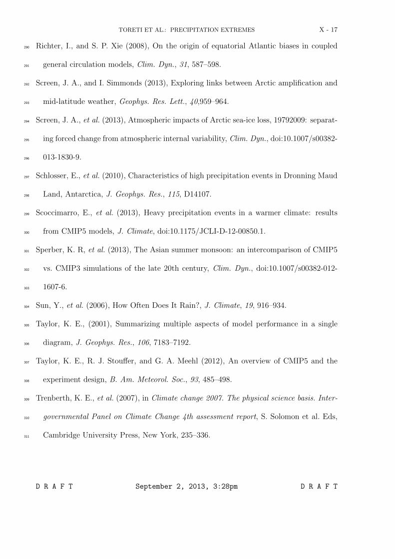
Figure 1. Ensemble mean 50-year return levels (mm) estimated for the period 1966-2005 in

boreal winter a and summer b. Blue coloured areas identify grid points where at least 75% of

the models pass the goodness-of-fit test (reliable points). Taylor diagrams for estimated 50-year

return levels in winter and summer over Northern Eurasia c,d and North America e,f. The full

symbols denote models with at least 75% of reliable grid points in the region.

Figure 2. Ensemble mean changes of the estimated 50-year return levels (%) with respect to

the period 1966-2005, under the RCP8.5 scenario for winter 2020-2059 a and 2060-2099 b and

summer 2020-2059 c and 2060-2099 d. Blue dots mark grid points where at least 75% of the

models pass the goodness-of-fit test and agree on the sign of the estimated changes.



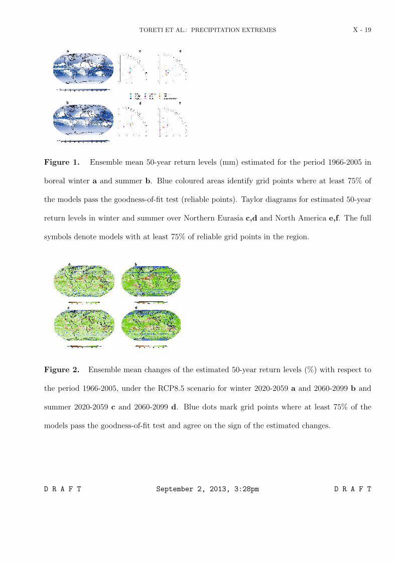
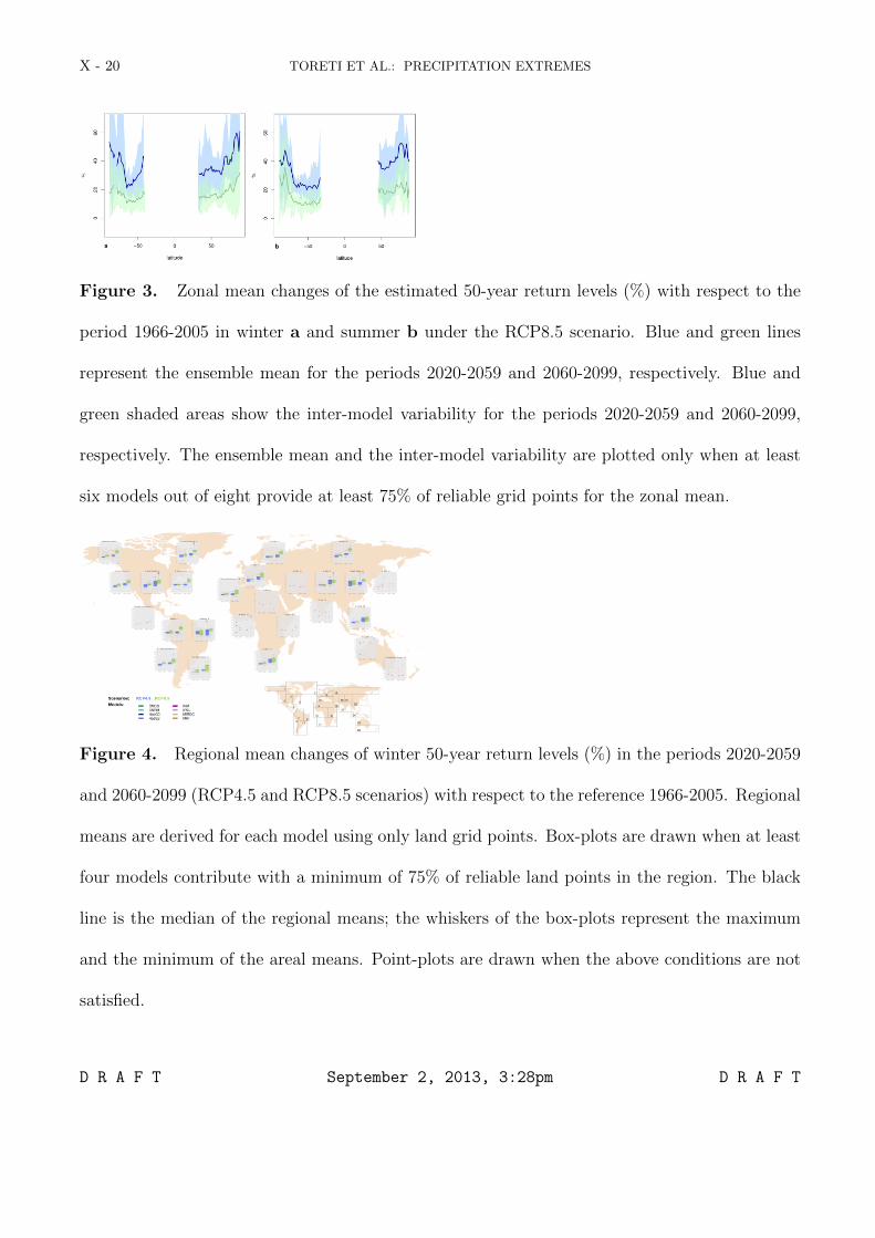
Figure 3. Zonal mean changes of the estimated 50-year return levels (%) with respect to the

period 1966-2005 in winter a and summer b under the RCP8.5 scenario. Blue and green lines

represent the ensemble mean for the periods 2020-2059 and 2060-2099, respectively. Blue and

green shaded areas show the inter-model variability for the periods 2020-2059 and 2060-2099,

respectively. The ensemble mean and the inter-model variability are plotted only when at least

six models out of eight provide at least 75% of reliable grid points for the zonal mean.

Figure 4. Regional mean changes of winter 50-year return levels (%) in the periods 2020-2059

and 2060-2099 (RCP4.5 and RCP8.5 scenarios) with respect to the reference 1966-2005. Regional

means are derived for each model using only land grid points. Box-plots are drawn when at least

four models contribute with a minimum of 75% of reliable land points in the region. The black

line is the median of the regional means; the whiskers of the box-plots represent the maximum

and the minimum of the areal means. Point-plots are drawn when the above conditions are not

satisfied.


projections of global changes in precipitation

Documents