processor architecture needed to handle fft algoarithm
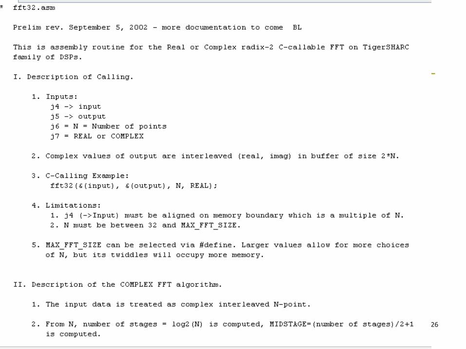
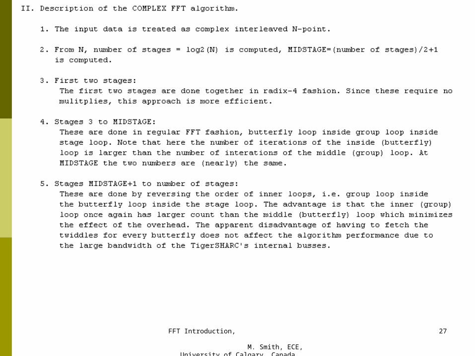
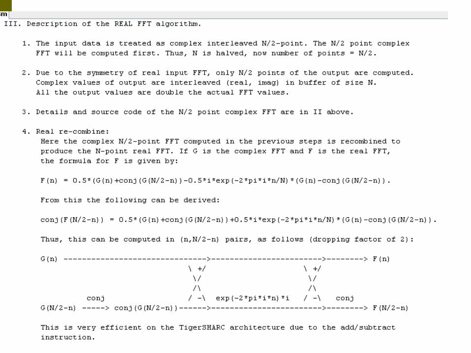
DESCRIPTION
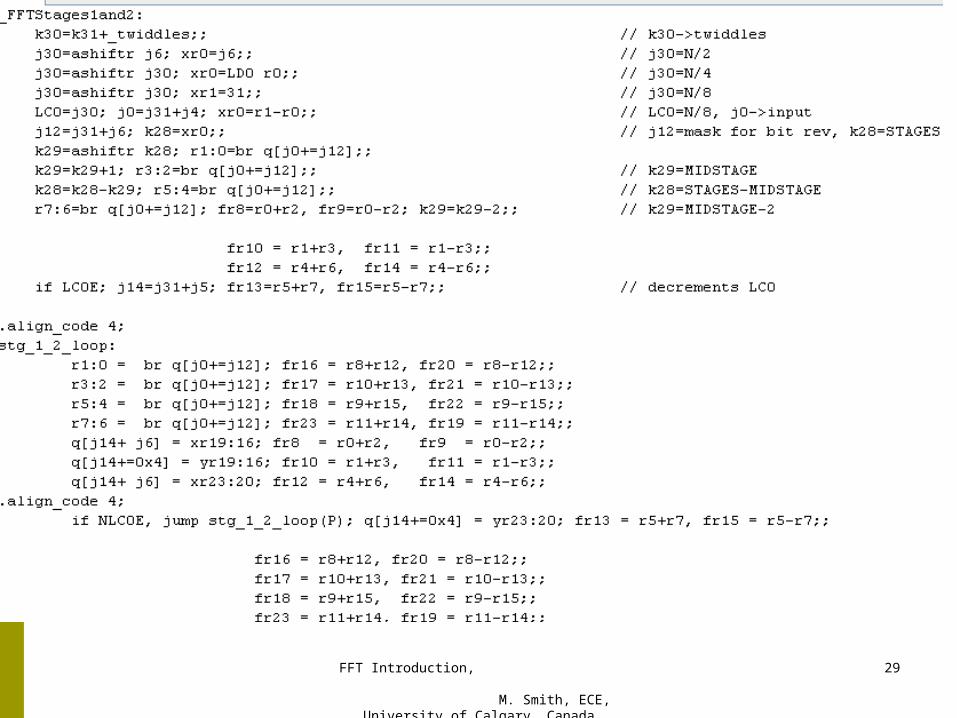
Processor Architecture Needed to handle FFT algoarithm. M. Smith. Tackled already this term. Three types of DSP algorithms Long loops, multiplication and addition intensive, regular (simple) memory accesses – e.g. 300 taps in FIR algorithms - PowerPoint PPT PresentationTRANSCRIPT
Processor Architecture
Needed to handleFFT algoarithm
M. Smith
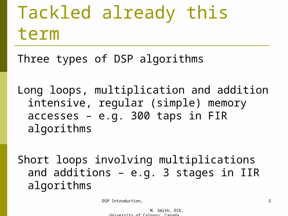
Tackled already this termThree types of DSP algorithms
Long loops, multiplication and addition intensive, regular (simple) memory accesses – e.g. 300 taps in FIR algorithms
Short loops involving multiplications and additions – e.g. 3 stages in IIR algorithms
DSP Introduction, M. Smith, ECE,
University of Calgary, Canada
2
DSP Introduction, M. Smith, ECE,
University of Calgary, Canada
3
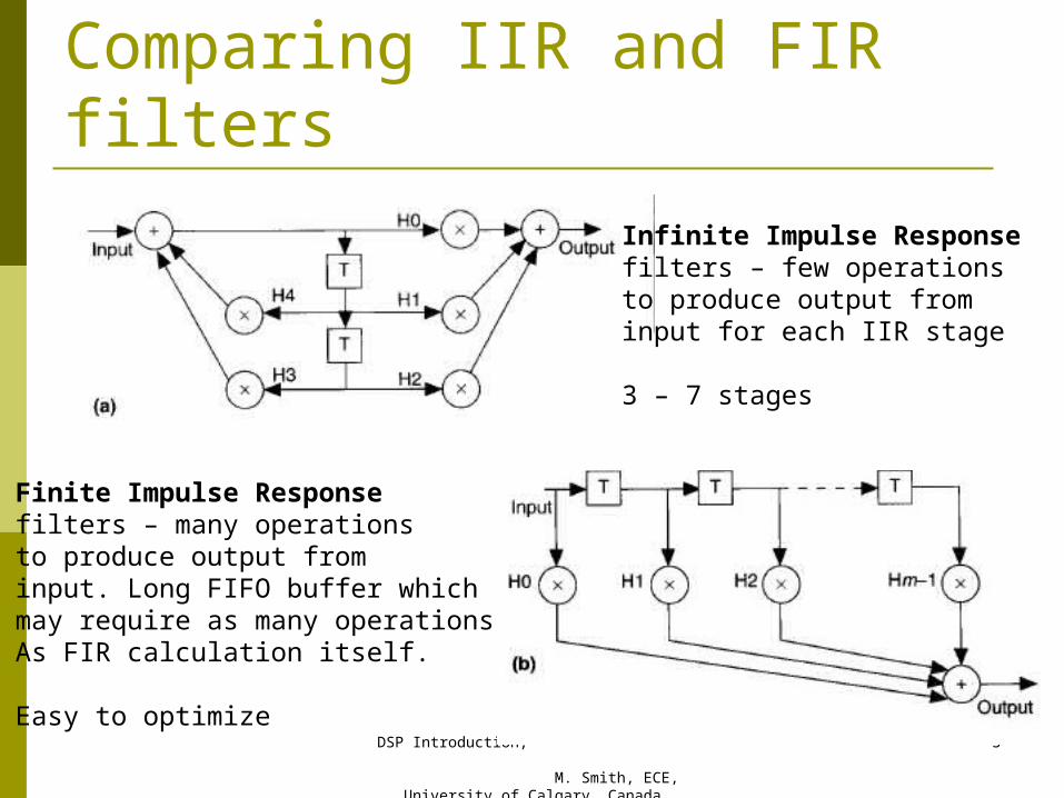
Comparing IIR and FIR filters
Infinite Impulse Responsefilters – few operations to produce output frominput for each IIR stage
3 – 7 stages
Finite Impulse Responsefilters – many operations to produce output frominput. Long FIFO buffer whichmay require as many operationsAs FIR calculation itself.
Easy to optimize
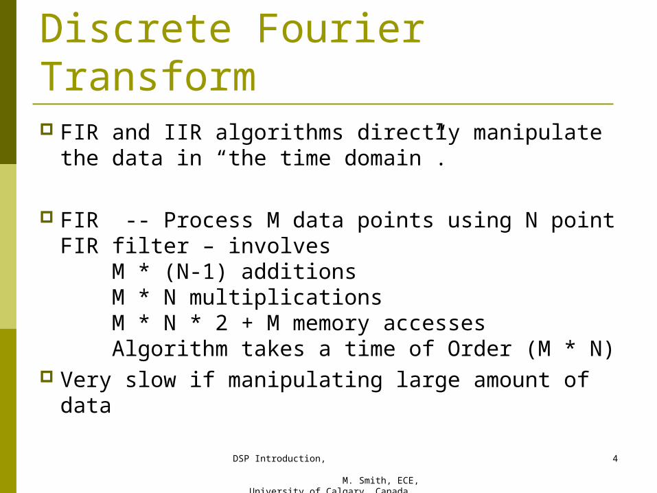
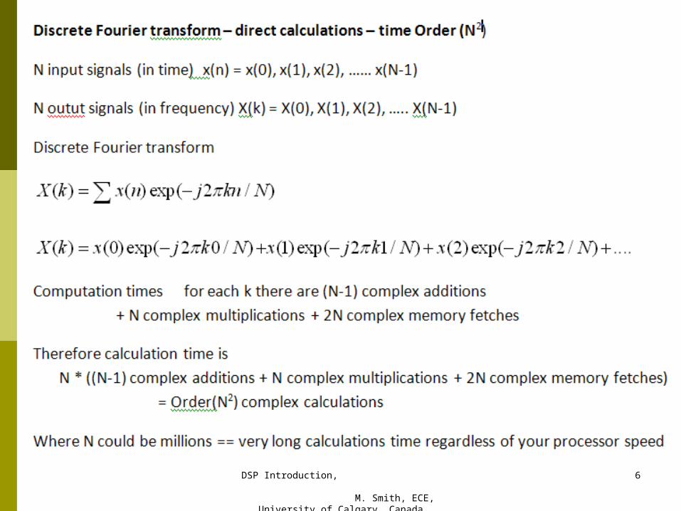
Discrete Fourier Transform FIR and IIR algorithms directly manipulate the
data in “the time domain”.
FIR -- Process M data points using N point FIR filter – involves M * (N-1) additions M * N multiplications M * N * 2 + M memory accesses Algorithm takes a time of Order (M * N)
Very slow if manipulating large amount of data
DSP Introduction, M. Smith, ECE,
University of Calgary, Canada
4
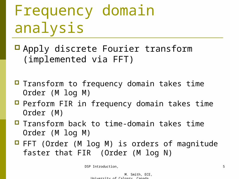
Frequency domain analysis Apply discrete Fourier transform
(implemented via FFT)
Transform to frequency domain takes time Order (M log M)
Perform FIR in frequency domain takes time Order (M)
Transform back to time-domain takes time Order (M log M)
FFT (Order (M log M) is orders of magnitude faster that FIR (Order (M log N)
DSP Introduction, M. Smith, ECE,
University of Calgary, Canada
5
DSP Introduction, M. Smith, ECE,
University of Calgary, Canada
6

DSP Introduction, M. Smith, ECE,
University of Calgary, Canada
7
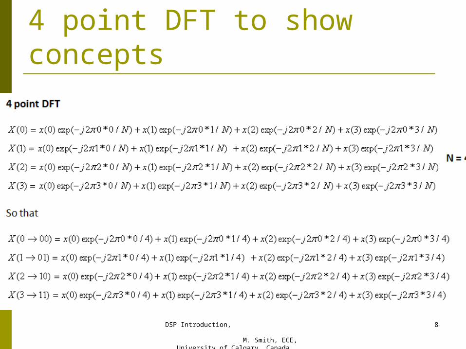
4 point DFT to show concepts
DSP Introduction, M. Smith, ECE,
University of Calgary, Canada
8
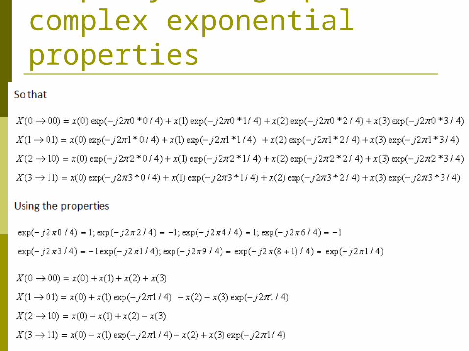
Simplify using special complex exponential properties
DSP Introduction, M. Smith, ECE,
University of Calgary, Canada
9
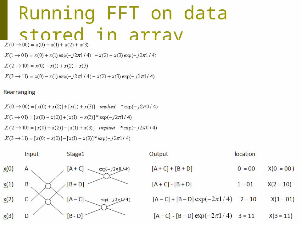
Running FFT on data stored in array
DSP Introduction, M. Smith, ECE,
University of Calgary, Canada
10
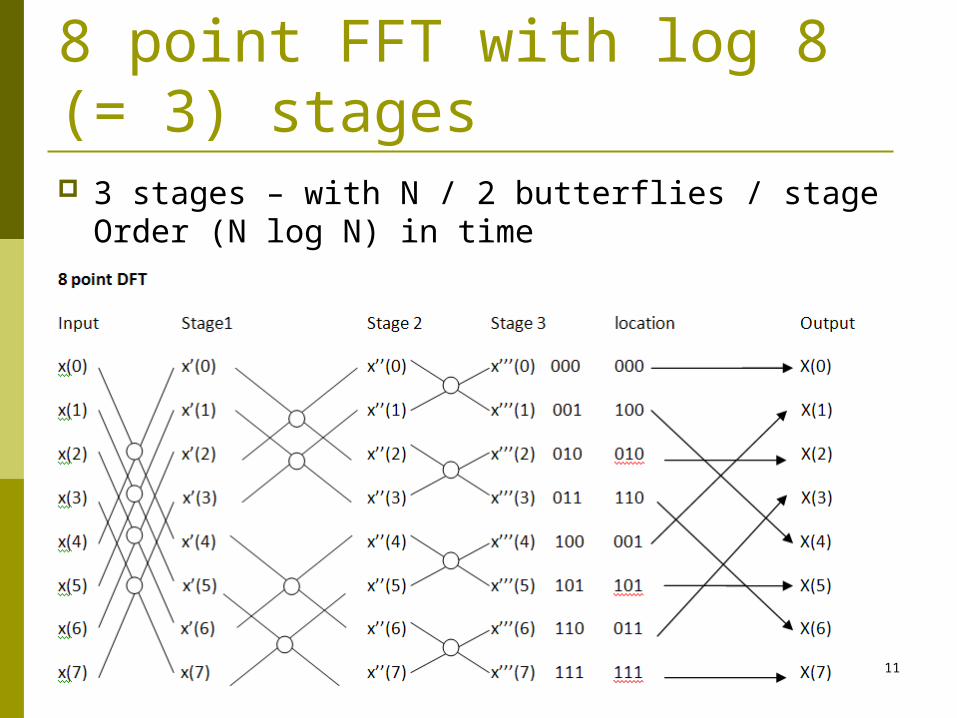
8 point FFT with log 8 (= 3) stages 3 stages – with N / 2 butterflies / stage
Order (N log N) in time
DSP Introduction, M. Smith, ECE,
University of Calgary, Canada
11
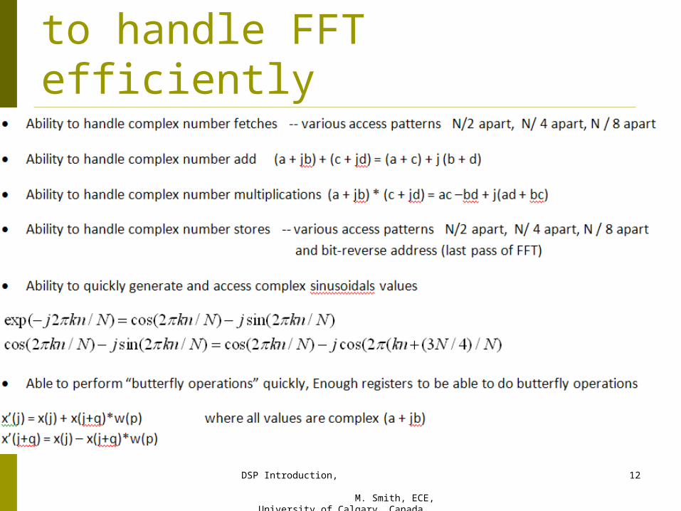
Architectural characteristics needed to handle FFT efficiently
DSP Introduction, M. Smith, ECE,
University of Calgary, Canada
12
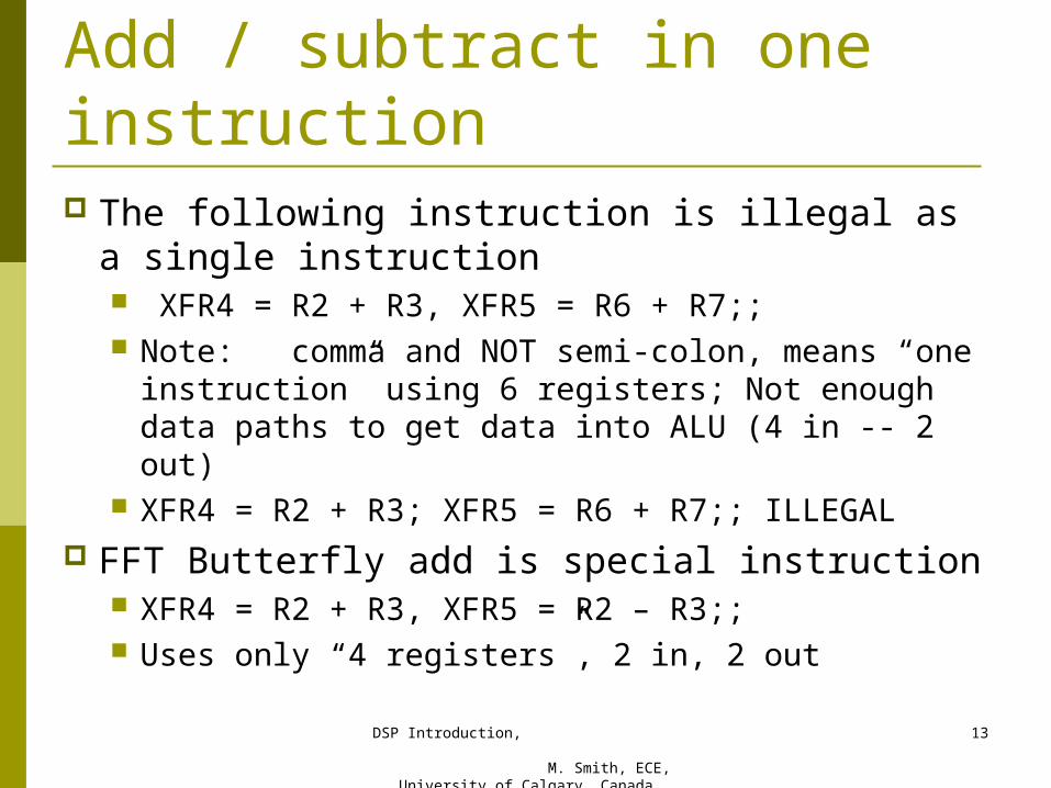
Add / subtract in one instruction The following instruction is illegal as a
single instruction XFR4 = R2 + R3, XFR5 = R6 + R7;; Note: comma and NOT semi-colon, means
“one instruction” using 6 registers; Not enough data paths to get data into ALU (4 in -- 2 out)
XFR4 = R2 + R3; XFR5 = R6 + R7;; ILLEGAL FFT Butterfly add is special instruction
XFR4 = R2 + R3, XFR5 = R2 – R3;; Uses only “4 registers”, 2 in, 2 out
DSP Introduction, M. Smith, ECE,
University of Calgary, Canada
13
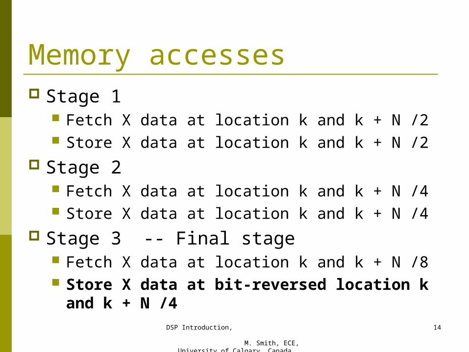
Memory accesses Stage 1
Fetch X data at location k and k + N /2 Store X data at location k and k + N /2
Stage 2 Fetch X data at location k and k + N /4 Store X data at location k and k + N /4
Stage 3 -- Final stage Fetch X data at location k and k + N /8 Store X data at bit-reversed location k
and k + N /4DSP Introduction,
M. Smith, ECE, University of Calgary, Canada
14
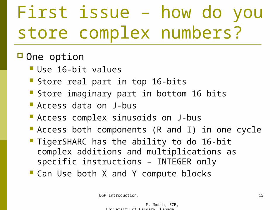
First issue – how do you store complex numbers? One option
Use 16-bit values Store real part in top 16-bits Store imaginary part in bottom 16 bits Access data on J-bus Access complex sinusoids on J-bus Access both components (R and I) in one cycle TigerSHARC has the ability to do 16-bit complex
additions and multiplications as specific instructions – INTEGER only
Can Use both X and Y compute blocksDSP Introduction,
M. Smith, ECE, University of Calgary, Canada
15
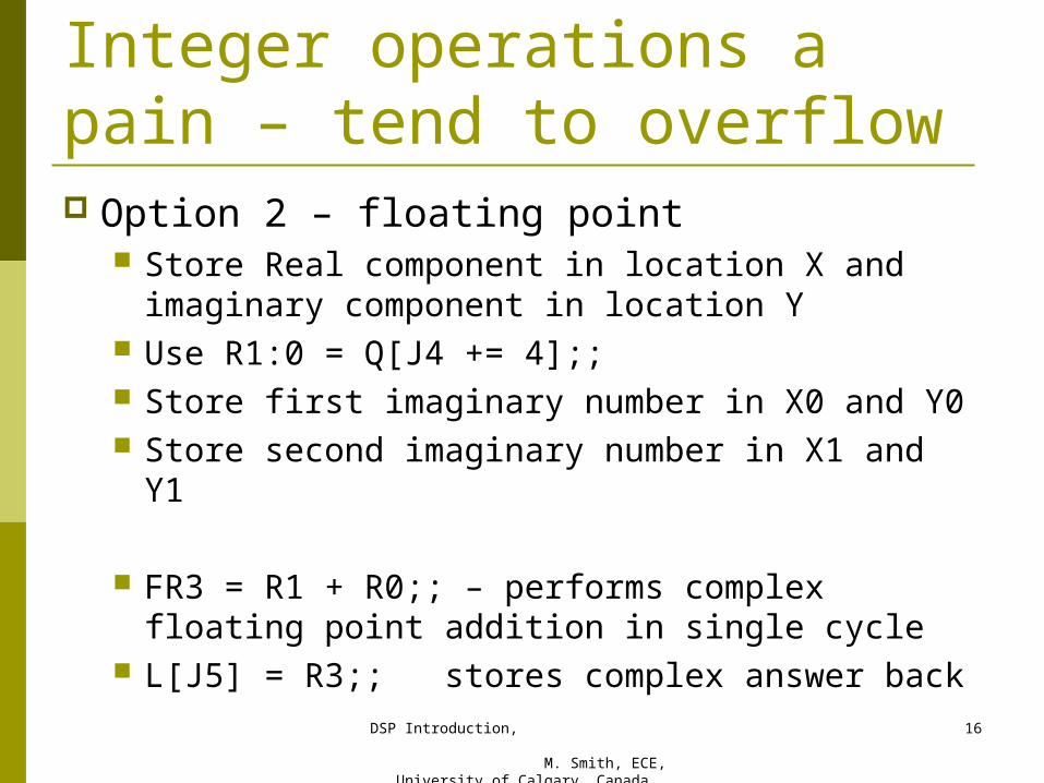
Integer operations a pain – tend to overflow Option 2 – floating point
Store Real component in location X and imaginary component in location Y
Use R1:0 = Q[J4 += 4];; Store first imaginary number in X0 and Y0 Store second imaginary number in X1 and Y1
FR3 = R1 + R0;; – performs complex floating point addition in single cycle
L[J5] = R3;; stores complex answer back
DSP Introduction, M. Smith, ECE,
University of Calgary, Canada
16
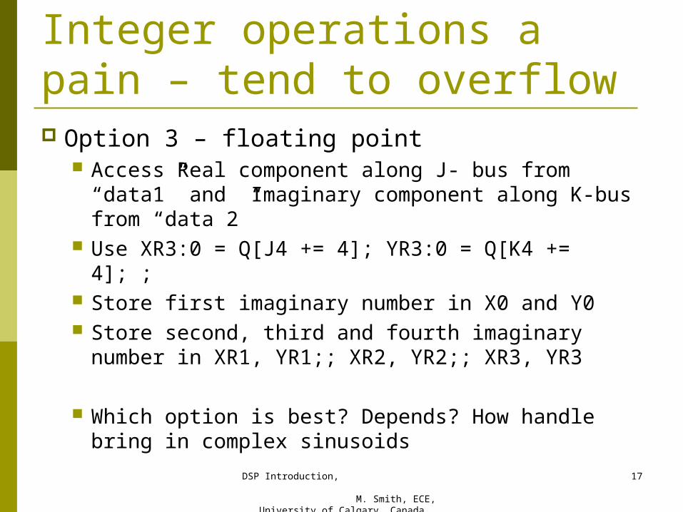
Integer operations a pain – tend to overflow Option 3 – floating point
Access Real component along J- bus from “data1” and Imaginary component along K-bus from “data 2”
Use XR3:0 = Q[J4 += 4]; YR3:0 = Q[K4 += 4]; ; Store first imaginary number in X0 and Y0 Store second, third and fourth imaginary
number in XR1, YR1;; XR2, YR2;; XR3, YR3
Which option is best? Depends? How handle bring in complex sinusoids
DSP Introduction, M. Smith, ECE,
University of Calgary, Canada
17
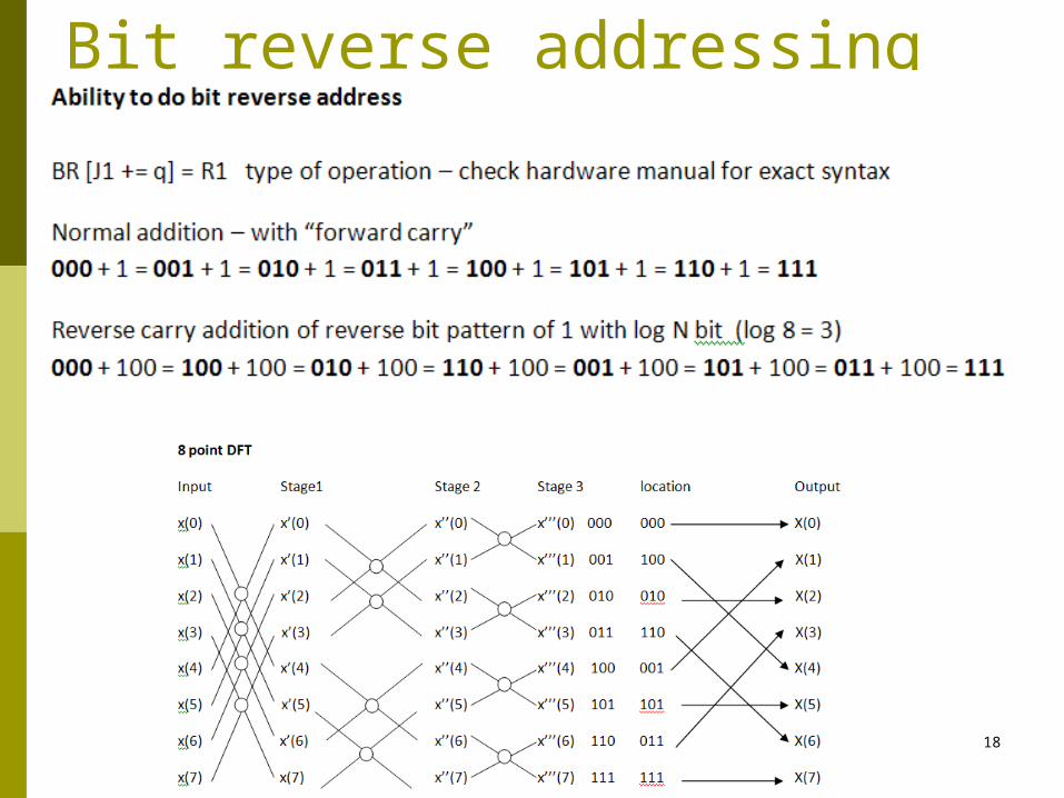
Bit reverse addressing
DSP Introduction, M. Smith, ECE,
University of Calgary, Canada
18
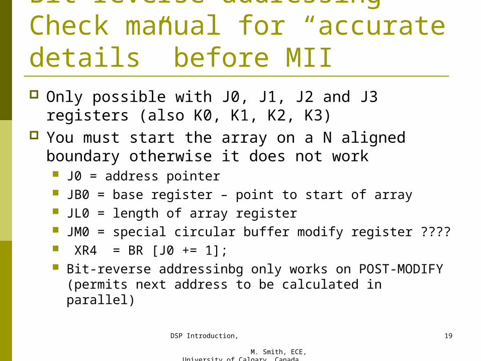
Bit reverse addressing – Check manual for “accurate details” before MII Only possible with J0, J1, J2 and J3 registers (also
K0, K1, K2, K3) You must start the array on a N aligned boundary
otherwise it does not work J0 = address pointer JB0 = base register – point to start of array JL0 = length of array register JM0 = special circular buffer modify register ???? XR4 = BR [J0 += 1]; Bit-reverse addressinbg only works on POST-MODIFY
(permits next address to be calculated in parallel)
DSP Introduction, M. Smith, ECE,
University of Calgary, Canada
19
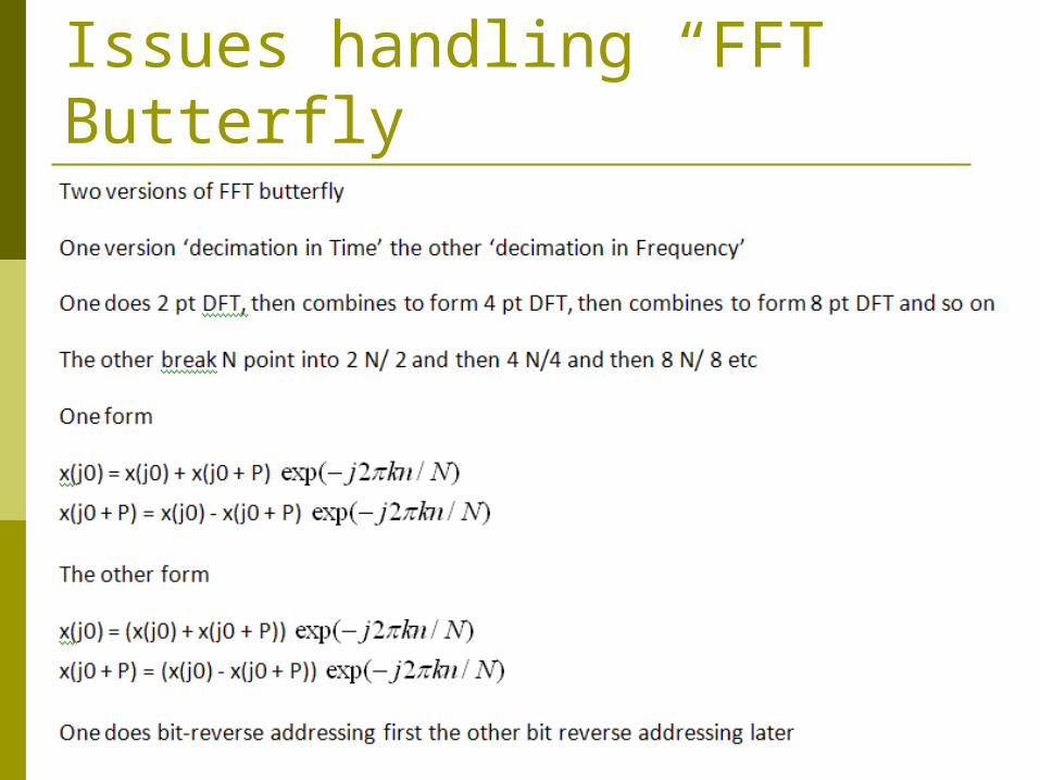
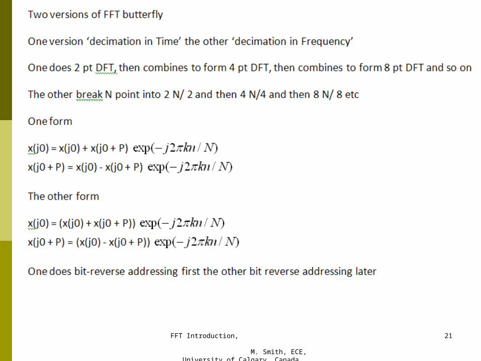
Issues handling “FFT Butterfly
DSP Introduction, M. Smith, ECE,
University of Calgary, Canada
20
FFT Introduction, M. Smith, ECE,
University of Calgary, Canada
21
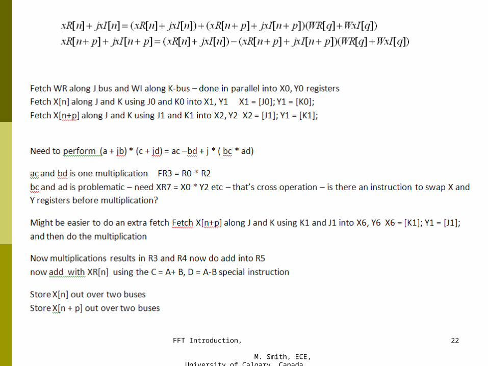
FFT Introduction, M. Smith, ECE,
University of Calgary, Canada
22
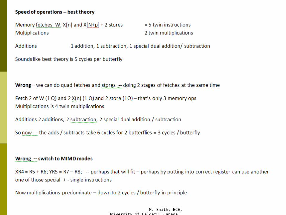
FFT Introduction, M. Smith, ECE,
University of Calgary, Canada
23
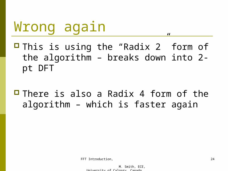
Wrong again This is using the “Radix 2” form of the
algorithm – breaks down into 2-pt DFT
There is also a Radix 4 form of the algorithm – which is faster again
FFT Introduction, M. Smith, ECE,
University of Calgary, Canada
24
FFT Introduction, M. Smith, ECE,
University of Calgary, Canada
25
FFT Introduction, M. Smith, ECE,
University of Calgary, Canada
26
FFT Introduction, M. Smith, ECE,
University of Calgary, Canada
27
FFT Introduction, M. Smith, ECE,
University of Calgary, Canada
28
FFT Introduction, M. Smith, ECE,
University of Calgary, Canada
29
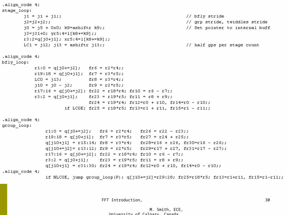
FFT Introduction, M. Smith, ECE,
University of Calgary, Canada
30
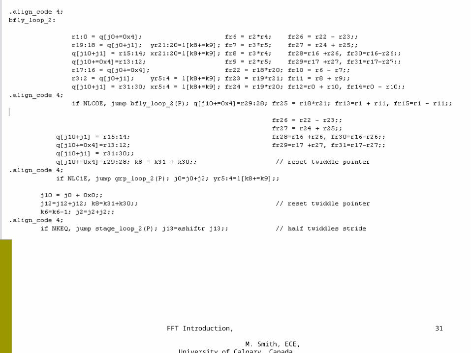
FFT Introduction, M. Smith, ECE,
University of Calgary, Canada
31
Many special TigerSHARC features to handle FFT
FFT Introduction, M. Smith, ECE,
University of Calgary, Canada
32