31

2 FFT ALGORITHMS

2.1 General

In FFT processor design, the mathematical properties of FFT must be exploited for

an efficient implementation since the selection of FFT algorithm has large impact

on the implementation in term of speed, hardware complexity, power consumption

etc. This chapter focuses on the review of FFT algorithms.

2.2 Cooley-Tukey FFT Algorithms

The techniques for efficient computation of DFTs is based on divide and conquer

approach. This technique works by recursively breaking down a problem into two,

or more, sub-problems of the same (or related) type. The sub-problems are then

independently solved and their solutions are combined to give a solution to the

original problem. This technique can be applied to DFT computation by dividing

the data sequence into smaller data sequences until the DFTs for small data

sequences can be computed efficiently. Although the technique was described in

1805 [46], it was not applied to DFT computation until 1965 [47]. Cooley and

Tukey demonstrated the simplicity and efficiency of the divide and conquer

approach for DFT computation and made the FFT algorithms widely accepted. We

give a simple example for the divide and conquer approach. Then a basic and a

generalized FFT formulation are given [47].

2.2.1 Eight point DFT

In this section, we illustrate the idea of the divide and conquer approach and show

why dividing is also conquering for DFT computation.

32

Let us consider an 8-point DFT, e.g., N=8 and data sequence {x(k)}, k= 0,1,…..7,

the DFT of the {x(k)} is given by

.7,.....1,0,][][ 8

7

0

nforWkxnX nk

k

(2.1)

One way to break down a long data sequence into shorter ones is to group the data

sequence according to their indices. Let{xo(l)} and {xe(l)} (l = 0, 1, 2, 3) be two

sequences, the grouping of {x(k)}to {xo(l)} and {xe(l)} and can be done intuitively

through separating members by odd and even index.

xo(l) = x(2l + 1) (2.2)

xe(l) = x(2l) (2.3)

for l = 0, 1, 2, 3

The DFT for{x(k)} can be rewritten

)2(

8

3

0

)12(

8

3

0

0 ][][][ ln

l

e

ln

l

WlxWlxnX

(2.4)

=)2(

8

3

0

)2(

88

3

0

0 ][][ ln

l

e

lnn

l

WlxWWlx

= nl

l

e

nl

l

WlxWlx 4

3

0

4

3

0

0 ][][

= )()(08 nXnXW e

n

where

)(

4

2)2(

8

2

)2(

8

lnlnln eeW

)(, 04 nXW nland )(nX e are

4-points DFTs of {xo(l)} and {xe(l)} respectively.

33

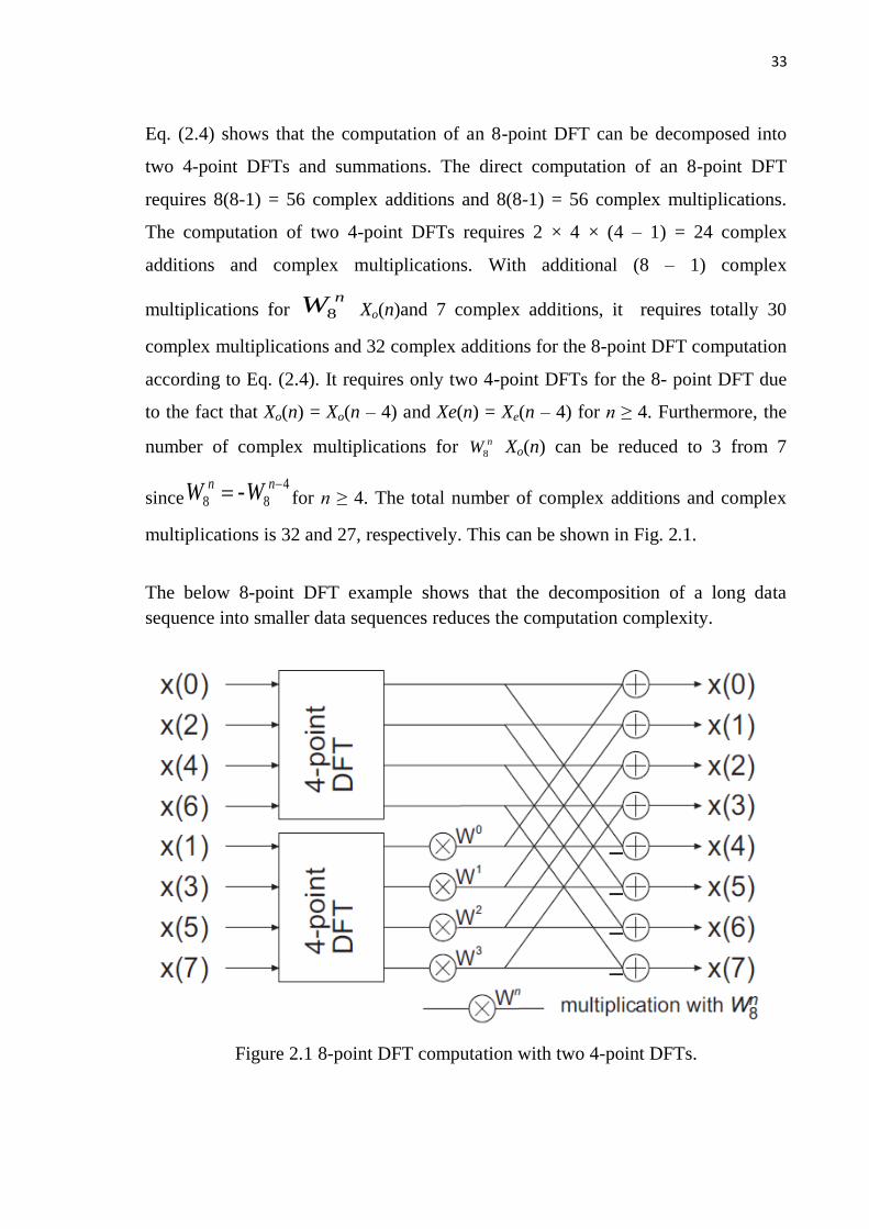
Eq. (2.4) shows that the computation of an 8-point DFT can be decomposed into

two 4-point DFTs and summations. The direct computation of an 8-point DFT

requires 8(8-1) = 56 complex additions and 8(8-1) = 56 complex multiplications.

The computation of two 4-point DFTs requires 2 × 4 × (4 – 1) = 24 complex

additions and complex multiplications. With additional (8 – 1) complex

multiplications for nW8 Xo(n)and 7 complex additions, it requires totally 30

complex multiplications and 32 complex additions for the 8-point DFT computation

according to Eq. (2.4). It requires only two 4-point DFTs for the 8- point DFT due

to the fact that Xo(n) = Xo(n – 4) and Xe(n) = Xe(n – 4) for n ≥ 4. Furthermore, the

number of complex multiplications for nW8 Xo(n) can be reduced to 3 from 7

since4

88 - nn WW for n ≥ 4. The total number of complex additions and complex

multiplications is 32 and 27, respectively. This can be shown in Fig. 2.1.

The below 8-point DFT example shows that the decomposition of a long data

sequence into smaller data sequences reduces the computation complexity.

Figure 2.1 8-point DFT computation with two 4-point DFTs.

34

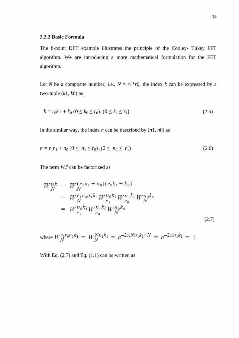
2.2.2 Basic Formula

The 8-point DFT example illustrates the principle of the Cooley- Tukey FFT

algorithm. We are introducing a more mathematical formulation for the FFT

algorithm.

Let N be a composite number, i.e., N = r1*r0, the index k can be expressed by a

two-tuple (k1, k0) as

k = r0k1 + k0 (0 ≤ k0 ≤ r0), (0 ≤ k1 ≤ r1) (2.5)

In the similar way, the index n can be described by (n1, n0) as

n = r1n1 + n0 (0 ≤ n1 ≤ r0) ,(0 ≤ n0 ≤ r1) (2.6)

The term nk

NW can be factorized as

(2.7)

where

With Eq. (2.7) and Eq. (1.1) can be written as

35

(2.8)

Eq. (2.8) indicates that the DFT computation can be performed in three steps:

Compute r0 different r1-point DFTs (inner parenthesis).

Multiply results with .

Compute r0 different r1-point DFTs (utter parenthesis).

The r0 r1-point DFTs require r0 r1 (r1 – 1) or N(r1 – 1) complex multiplications and

additions. The second step requires N complex multiplications. The final step

requires N (r0 – 1) complex multiplications and additions. Therefore the total

number of complex multiplications using Eq. (2.8) is N (r0+ r1 – 1) and the number

of complex additions is N (r0+ r1 – 2) . This is a reduction from O(N2) to O(N(r1

+r0)). Therefore the decomposition of DFT reduces the computation complexity for

DFT.

The number r0 and r1 are called radix. If r0 and r1 are equal to r, the number system

is called radix-r system. Otherwise, it is called mixed-radix system. The

multiplications with are called twiddle factor multiplications.

Example 2.1 For N= 8, we apply the basic formula by decomposing N = 8 = 4*2

with r0 = 2 and r1 = 4. This results in the given 8-point DFT example in the above

section, which is shown in Fig. 2.1. It is a mixed-radix FFT algorithm. A closer

study for the given 8-point DFT example, it is easy to show that it does not need to

store the input data in the memory after the computation of the two 4-point DFTs. It

can reduce the total memory size and is important for memory constrained system.

An algorithm with this property is called an in-place algorithm.

36

2.2.3 Generalized Formula

If r0 or/and r1 are not prime, further improvement to reduce the computation

complexity can be achieved by applying the divide and conquer approach

recursively to r1-point or/and r0-point DFTs [48].

Let N = r p – 1 r p – 2 * ¼ * r0, the index k and n can be written as

(2.9) & (2.10)

where

The factorization of nk

NW can be expressed as

(2.11)

where

Eq. (2.1) can then be written

(2.12)

37

Note that the inner product can be recognized as an rp-1-point DFT for n0. Define

(2.13)

With Eq. (2.13), index kp-1 is “replaced” by n0. Equation (2.12) can now be

rewritten as

(2.14)

The term can be factorized as

The inner sum of kp-2 in Eq. (2.14) can then be written as

38

(2.15)

which can be done through multiplications and rp-2-point DFTs

Eq. (2.14) can be rewritten as

This process from Eq. (2.14) to Eq. (2.17) can be repeated p – 2 times until index k0

is replaced by np-1.

(2.19)

Eq. (2.14) can then be expressed as

(2.20)

(2.16)

(2.17)

(2.18)

39

Eq. (2.20) reorders the output data to natural order. This process is called

unscrambling. The unscrambling process requires a special addressing mode that

converts address (n0,...,np-1) to (np – 1, np – 2,…, n0). In case for radix-2 number

system, the ni represents a bit. The addressing for unscrambling is to make a reverse

of the address bits and hence is called bit-reverse addressing. In case of radix-r (r >

2) number system, it is called digit-reverse addressing.

Example 2.2 8-point DFT. Let N = 2 2, the factorization of nk

NW can be

expressed as

(2.21)

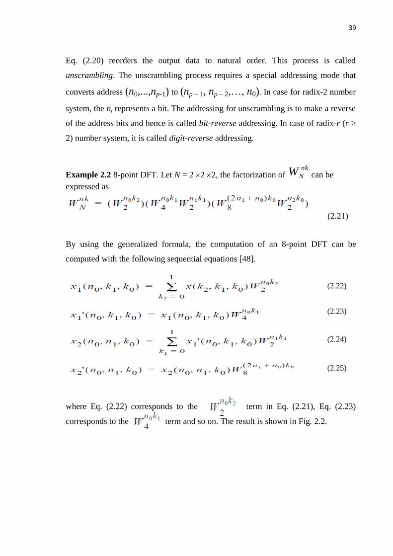
By using the generalized formula, the computation of an 8-point DFT can be

computed with the following sequential equations [48].

where Eq. (2.22) corresponds to the term in Eq. (2.21), Eq. (2.23)

corresponds to the term and so on. The result is shown in Fig. 2.2.

(2.22)

(2.23)

(2.24)

(2.25)

40

Figure 2.2 8-point DFT with Cooley-Tukey algorithm.

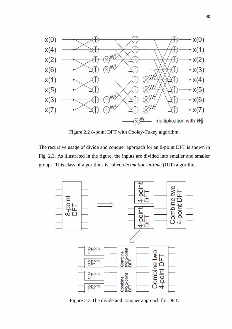
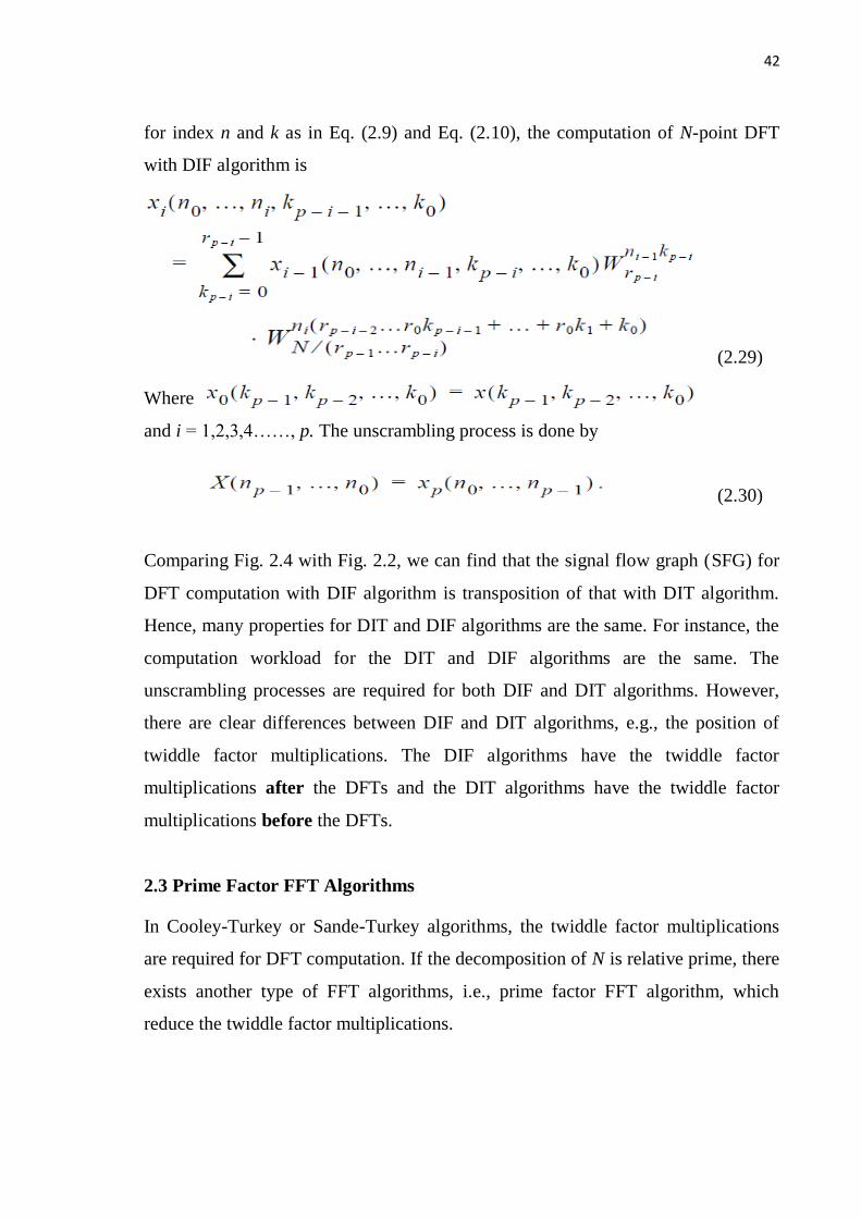
The recursive usage of divide and conquer approach for an 8-point DFT is shown in

Fig. 2.3. As illustrated in the figure, the inputs are divided into smaller and smaller

groups. This class of algorithms is called decimation-in-time (DIT) algorithm.

Figure 2.3 The divide and conquer approach for DFT.

41

2.2 Sande-Tukey FFT Algorithms

Another class of algorithms is called decimation-in-frequency (DIF) algorithm,

which divides the outputs into smaller and smaller DFTs. This kind of algorithm is

also called the Sande-Tukey FFT algorithm.

The computation of DFT with DIF algorithm is similar to computation with DIT

algorithm. For the sake of simplicity, we do not derive the DIF algorithm but

illustrate the algorithm with an example.

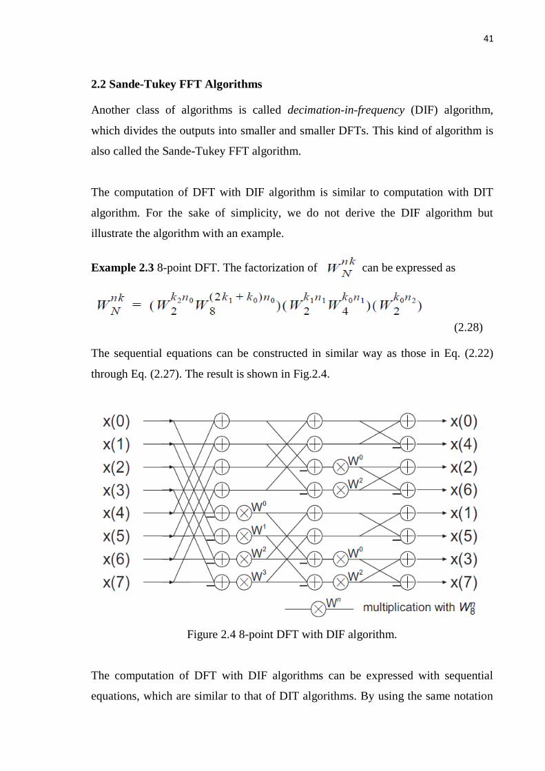
Example 2.3 8-point DFT. The factorization of can be expressed as

(2.28)

The sequential equations can be constructed in similar way as those in Eq. (2.22)

through Eq. (2.27). The result is shown in Fig.2.4.

Figure 2.4 8-point DFT with DIF algorithm.

The computation of DFT with DIF algorithms can be expressed with sequential

equations, which are similar to that of DIT algorithms. By using the same notation

42

for index n and k as in Eq. (2.9) and Eq. (2.10), the computation of N-point DFT

with DIF algorithm is

(2.29)

Where and

and i = 1,2,3,4……, p. The unscrambling process is done by

(2.30)

Comparing Fig. 2.4 with Fig. 2.2, we can find that the signal flow graph (SFG) for

DFT computation with DIF algorithm is transposition of that with DIT algorithm.

Hence, many properties for DIT and DIF algorithms are the same. For instance, the

computation workload for the DIT and DIF algorithms are the same. The

unscrambling processes are required for both DIF and DIT algorithms. However,

there are clear differences between DIF and DIT algorithms, e.g., the position of

twiddle factor multiplications. The DIF algorithms have the twiddle factor

multiplications after the DFTs and the DIT algorithms have the twiddle factor

multiplications before the DFTs.

2.3 Prime Factor FFT Algorithms

In Cooley-Turkey or Sande-Turkey algorithms, the twiddle factor multiplications

are required for DFT computation. If the decomposition of N is relative prime, there

exists another type of FFT algorithms, i.e., prime factor FFT algorithm, which

reduce the twiddle factor multiplications.

43

In Cooley-Turkey or Sande-Turkey algorithms, index n or k is expressed with Eq.

(2.9) and Eq. (2.10). This representation of index number is called index mapping.

If r1 and r1 are relatively prime, e.g., greatest common divider (GCD) (r1, r1) = 1, it

exists another index mapping, so-called Good’s mapping [19]. An index n can be

expressed as

(2.31)

where is the

multiplication inverse of modulo and

r1–1

is the multiplication inverse of r0 modulo . This mapping is a variant of Chinese

Remainder Theorem.

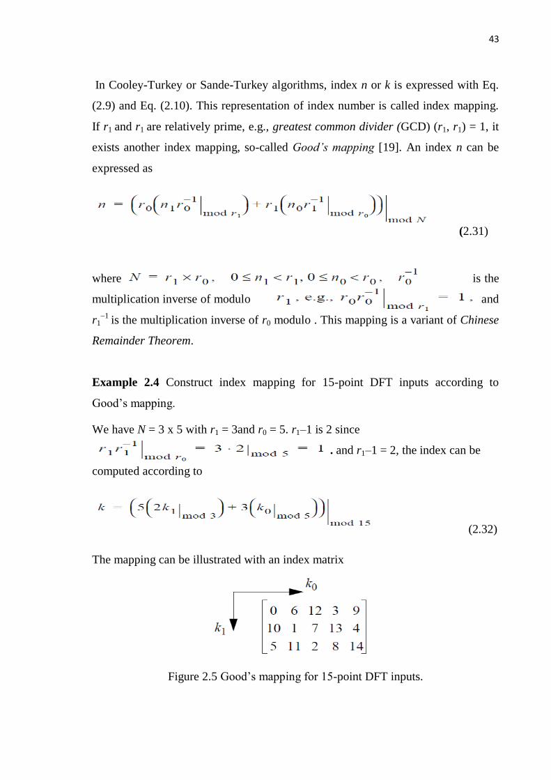
Example 2.4 Construct index mapping for 15-point DFT inputs according to

Good’s mapping.

We have N = 3 x 5 with r1 = 3and r0 = 5. r1–1 is 2 since

. and r1–1 = 2, the index can be

computed according to

(2.32)

The mapping can be illustrated with an index matrix

Figure 2.5 Good’s mapping for 15-point DFT inputs.

44

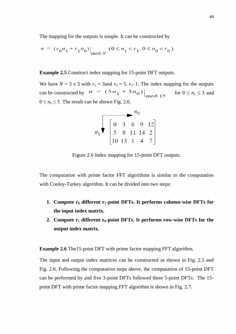
The mapping for the outputs is simple. It can be constructed by

Example 2.5 Construct index mapping for 15-point DFT outputs.

We have N = 3 x 5 with r1 = 3and r0 = 5. r1–1. The index mapping for the outputs

can be constructed by for 0 ≤ n1 ≤ 3 and

0 ≤ n0 ≤ 5. The result can be shown Fig. 2.6.

Figure 2.6 Index mapping for 15-point DFT outputs.

The computation with prime factor FFT algorithms is similar to the computation

with Cooley-Turkey algorithm. It can be divided into two steps:

1. Compute r0 different r1-point DFTs. It performs column-wise DFTs for

the input index matrix.

2. Compute r1 different r0-point DFTs. It performs row-wise DFTs for the

output index matrix.

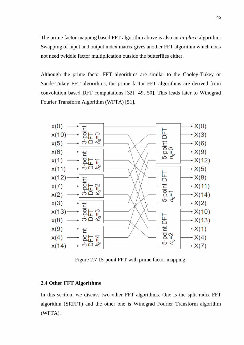
Example 2.6 The15-point DFT with prime factor mapping FFT algorithm.

The input and output index matrices can be constructed as shown in Fig. 2.5 and

Fig. 2.6. Following the computation steps above, the computation of 15-point DFT

can be performed by and five 3-point DFTs followed three 5-point DFTs. The 15-

point DFT with prime factor mapping FFT algorithm is shown in Fig. 2.7.

45

The prime factor mapping based FFT algorithm above is also an in-place algorithm.

Swapping of input and output index matrix gives another FFT algorithm which does

not need twiddle factor multiplication outside the butterflies either.

Although the prime factor FFT algorithms are similar to the Cooley-Tukey or

Sande-Tukey FFT algorithms, the prime factor FFT algorithms are derived from

convolution based DFT computations [32] [49, 50]. This leads later to Winograd

Fourier Transform Algorithm (WFTA) [51].

Figure 2.7 15-point FFT with prime factor mapping.

2.4 Other FFT Algorithms

In this section, we discuss two other FFT algorithms. One is the split-radix FFT

algorithm (SRFFT) and the other one is Winograd Fourier Transform algorithm

(WFTA).

46

2.4.1 Split-Radix FFT Algorithm

Split-radix FFT algorithms (SRFFT) were proposed nearly simultaneously by

several authors in 1984 [52] [53]. The algorithms belong to the FFT algorithms with

twiddle factor. As a matter of fact, split-radix FFT algorithms are based on the

observation of Cooley- Turkey and Sande-Turkey FFT algorithms. It is observed

that different decomposition can be used for different parts of an algorithm. This

gives possibility to select the most suitable algorithms for different parts in order to

reduce the computational complexity.

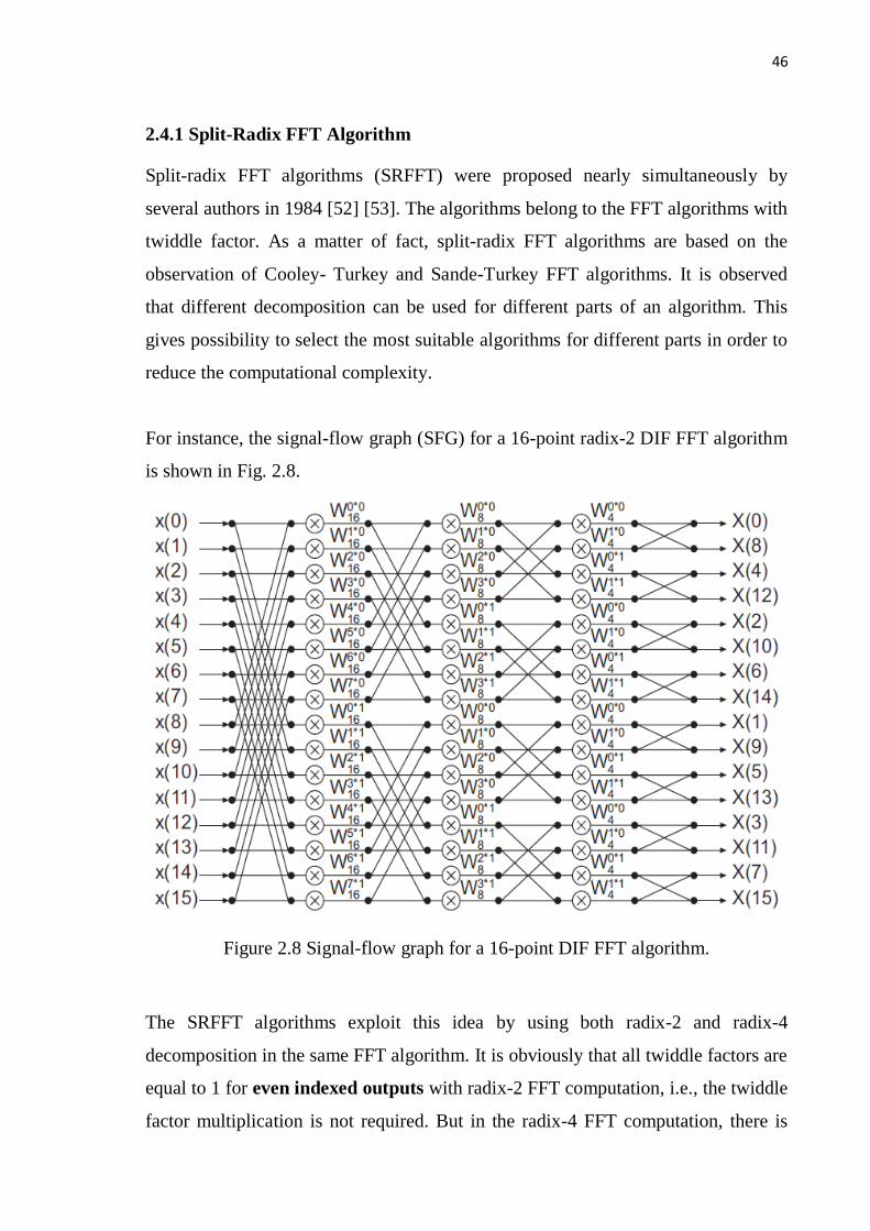
For instance, the signal-flow graph (SFG) for a 16-point radix-2 DIF FFT algorithm

is shown in Fig. 2.8.

Figure 2.8 Signal-flow graph for a 16-point DIF FFT algorithm.

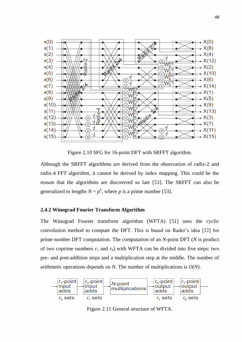
The SRFFT algorithms exploit this idea by using both radix-2 and radix-4

decomposition in the same FFT algorithm. It is obviously that all twiddle factors are

equal to 1 for even indexed outputs with radix-2 FFT computation, i.e., the twiddle

factor multiplication is not required. But in the radix-4 FFT computation, there is

47

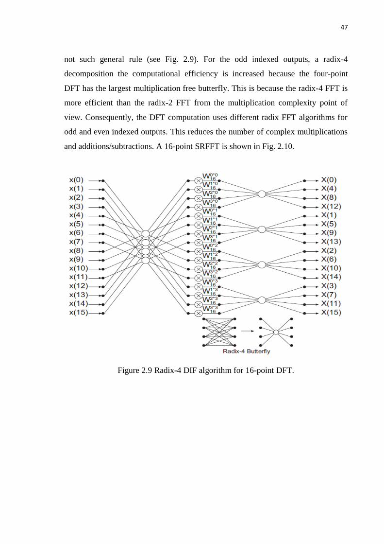
not such general rule (see Fig. 2.9). For the odd indexed outputs, a radix-4

decomposition the computational efficiency is increased because the four-point

DFT has the largest multiplication free butterfly. This is because the radix-4 FFT is

more efficient than the radix-2 FFT from the multiplication complexity point of

view. Consequently, the DFT computation uses different radix FFT algorithms for

odd and even indexed outputs. This reduces the number of complex multiplications

and additions/subtractions. A 16-point SRFFT is shown in Fig. 2.10.

Figure 2.9 Radix-4 DIF algorithm for 16-point DFT.

48

Figure 2.10 SFG for 16-point DFT with SRFFT algorithm.

Although the SRFFT algorithms are derived from the observation of radix-2 and

radix-4 FFT algorithm, it cannot be derived by index mapping. This could be the

reason that the algorithms are discovered so late [53]. The SRFFT can also be

generalized to lengths N = pk, where p is a prime number [53].

2.4.2 Winograd Fourier Transform Algorithm

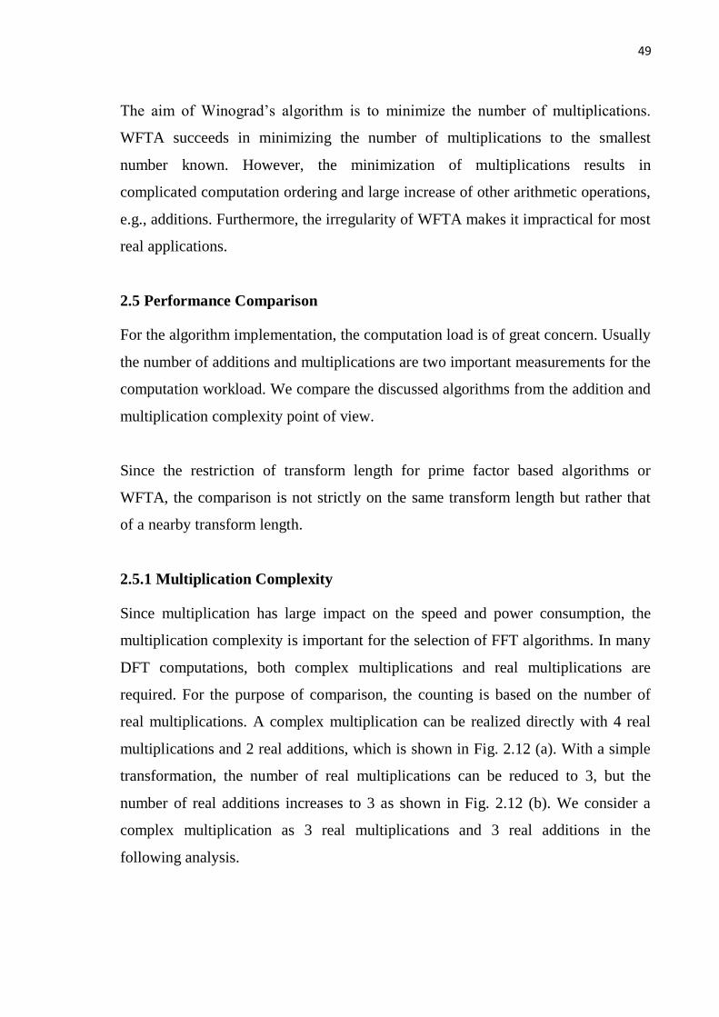
The Winograd Fourier transform algorithm (WFTA) [51] uses the cyclic

convolution method to compute the DFT. This is based on Rader’s idea [32] for

prime number DFT computation. The computation of an N-point DFT (N is product

of two coprime numbers r1 and r0) with WFTA can be divided into five steps: two

pre- and post-addition steps and a multiplication step at the middle. The number of

arithmetic operations depends on N. The number of multiplications is O(N).

Figure 2.11 General structure of WFTA.

49

The aim of Winograd’s algorithm is to minimize the number of multiplications.

WFTA succeeds in minimizing the number of multiplications to the smallest

number known. However, the minimization of multiplications results in

complicated computation ordering and large increase of other arithmetic operations,

e.g., additions. Furthermore, the irregularity of WFTA makes it impractical for most

real applications.

2.5 Performance Comparison

For the algorithm implementation, the computation load is of great concern. Usually

the number of additions and multiplications are two important measurements for the

computation workload. We compare the discussed algorithms from the addition and

multiplication complexity point of view.

Since the restriction of transform length for prime factor based algorithms or

WFTA, the comparison is not strictly on the same transform length but rather that

of a nearby transform length.

2.5.1 Multiplication Complexity

Since multiplication has large impact on the speed and power consumption, the

multiplication complexity is important for the selection of FFT algorithms. In many

DFT computations, both complex multiplications and real multiplications are

required. For the purpose of comparison, the counting is based on the number of

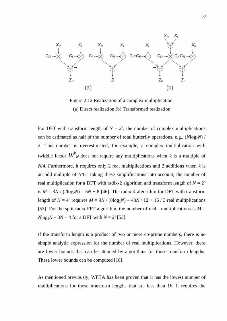
real multiplications. A complex multiplication can be realized directly with 4 real

multiplications and 2 real additions, which is shown in Fig. 2.12 (a). With a simple

transformation, the number of real multiplications can be reduced to 3, but the

number of real additions increases to 3 as shown in Fig. 2.12 (b). We consider a

complex multiplication as 3 real multiplications and 3 real additions in the

following analysis.

50

Figure 2.12 Realization of a complex multiplication.

(a) Direct realization (b) Transformed realization

For DFT with transform length of N = 2n, the number of complex multiplications

can be estimated as half of the number of total butterfly operations, e.g., (Nlog2N) /

2. This number is overestimated, for example, a complex multiplication with

twiddle factor WkN does not require any multiplications when k is a multiple of

N/4. Furthermore, it requires only 2 real multiplications and 2 additions when k is

an odd multiple of N/8. Taking these simplifications into account, the number of

real multiplication for a DFT with radix-2 algorithm and transform length of N = 2n

is M = 3N / (2log2N) – 5N + 8 [46]. The radix-4 algorithm for DFT with transform

length of N = 4n requires M = 9N / (8log2N) – 43N / 12 + 16 / 3 real multiplications

[53]. For the split-radix FFT algorithm, the number of real multiplications is M =

Nlog2N – 3N + 4 for a DFT with N = 2n

[53].

If the transform length is a product of two or more co-prime numbers, there is no

simple analytic expression for the number of real multiplications. However, there

are lower bounds that can be attained by algorithms for those transform lengths.

These lower bounds can be computed [18].

As mentioned previously, WFTA has been proven that it has the lowest number of

multiplications for those transform lengths that are less than 16. It requires the

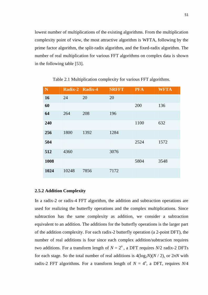
51

lowest number of multiplications of the existing algorithms. From the multiplication

complexity point of view, the most attractive algorithm is WFTA, following by the

prime factor algorithm, the split-radix algorithm, and the fixed-radix algorithm. The

number of real multiplication for various FFT algorithms on complex data is shown

in the following table [53].

Table 2.1 Multiplication complexity for various FFT algorithms.

N Radix-2 Radix-4 SRFFT PFA WFTA

16 24 20 20

60 200 136

64 264 208 196

240 1100 632

256 1800 1392 1284

504 2524 1572

512 4360 3076

1008 5804 3548

1024 10248 7856 7172

2.5.2 Addition Complexity

In a radix-2 or radix-4 FFT algorithm, the addition and subtraction operations are

used for realizing the butterfly operations and the complex multiplications. Since

subtraction has the same complexity as addition, we consider a subtraction

equivalent to an addition. The additions for the butterfly operations is the larger part

of the addition complexity. For each radix-2 butterfly operation (a 2-point DFT), the

number of real additions is four since each complex addition/subtraction requires

two additions. For a transform length of N = 2n

, a DFT requires N/2 radix-2 DFTs

for each stage. So the total number of real additions is 4(log2N)(N / 2), or 2nN with

radix-2 FFT algorithms. For a transform length of N = 4n, a DFT, requires N/4

52

radix-4 DFTs for each stage. Each radix-4 DFT requires 8 complex

additions/subtractions, i.e., 16 real additions. The total number of real additions is

16(log4N)(N / 4), or 4nN . Both radix-2 and radix-4 FFT algorithms require the

same number of additions for a DFT with a transform length of powers of 4.

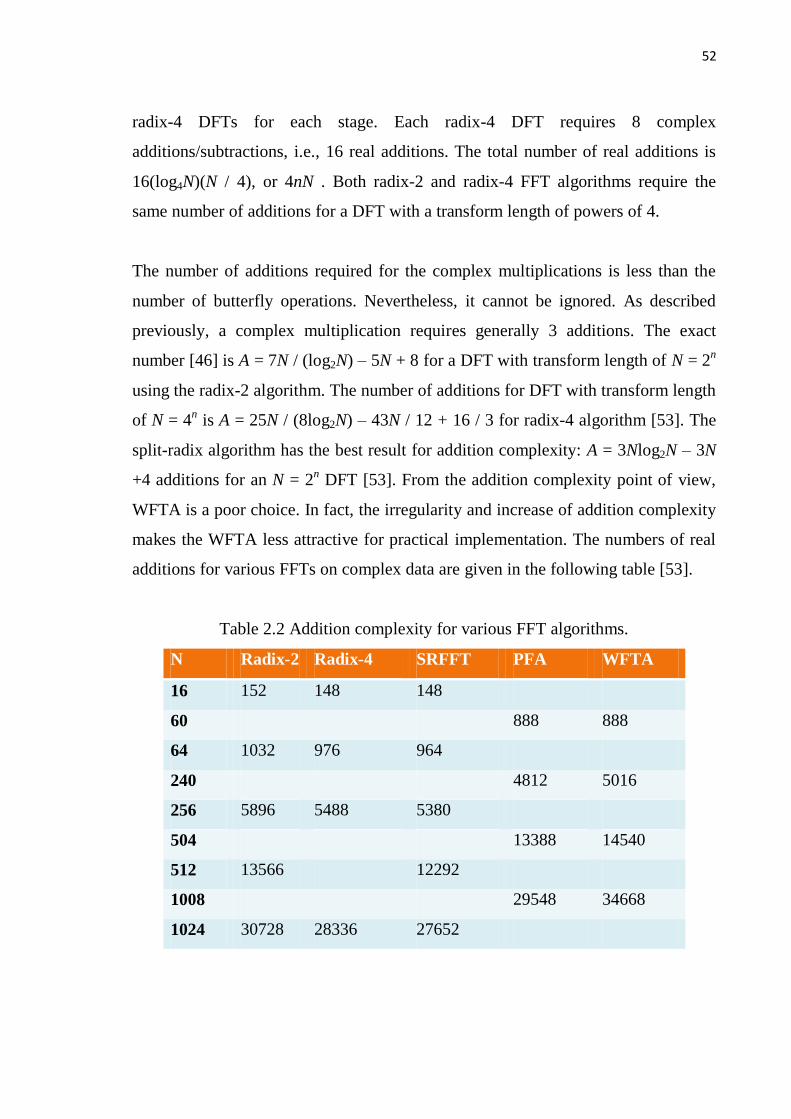
The number of additions required for the complex multiplications is less than the

number of butterfly operations. Nevertheless, it cannot be ignored. As described

previously, a complex multiplication requires generally 3 additions. The exact

number [46] is A = 7N / (log2N) – 5N + 8 for a DFT with transform length of N = 2n

using the radix-2 algorithm. The number of additions for DFT with transform length

of N = 4n is A = 25N / (8log2N) – 43N / 12 + 16 / 3 for radix-4 algorithm [53]. The

split-radix algorithm has the best result for addition complexity: A = 3Nlog2N – 3N

+4 additions for an N = 2n DFT [53]. From the addition complexity point of view,

WFTA is a poor choice. In fact, the irregularity and increase of addition complexity

makes the WFTA less attractive for practical implementation. The numbers of real

additions for various FFTs on complex data are given in the following table [53].

Table 2.2 Addition complexity for various FFT algorithms.

N Radix-2 Radix-4 SRFFT PFA WFTA

16 152 148 148

60 888 888

64 1032 976 964

240 4812 5016

256 5896 5488 5380

504 13388 14540

512 13566 12292

1008 29548 34668

1024 30728 28336 27652

53

2.6 Other Issues

Many issues are related to the FFT algorithm implementations, e.g., scaling and

rounding considerations, inverse FFT implementation, parallelism of FFT

algorithms, in-place and/or in-order issue, regularity of FFT algorithms etc. We

discuss the first two issues in more detail.

2.6.1 Scaling and Rounding Issue

In hardware it is not possible to implement an algorithm with infinite accuracy. To

obtain sufficient accuracy, the scaling and rounding effects must be considered.

Without loss of generality, we assume that the input data {x(n)} are scaled, i.e.,

|x(n)| < 1/2, for all n. To avoid overflow of the number range, we apply the safe

scaling technique [51]. This ensures that an overflow cannot occur. We take the 16-

point DFT with radix-2 DIF FFT algorithm (see Fig. 2.8) as an example.

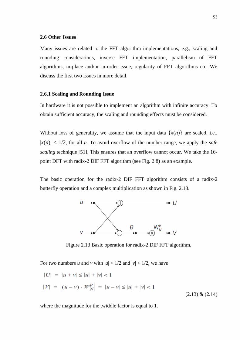
The basic operation for the radix-2 DIF FFT algorithm consists of a radix-2

butterfly operation and a complex multiplication as shown in Fig. 2.13.

Figure 2.13 Basic operation for radix-2 DIF FFT algorithm.

For two numbers u and v with |u| < 1/2 and |v| < 1/2, we have

(2.13) & (2.14)

where the magnitude for the twiddle factor is equal to 1.

54

To retain the magnitude, the results must be scaled with a factor 1/2. After scaling,

rounding is applied in order to have the same input and output wordlengths. This

introduces an error, which is called quantization noise. This noise for a real number

is modeled as an additive white noise source with zero mean and variance of Δ2/12,

where Δ is the weight of the least significant bit.

Figure 2.14 Model for scaling and rounding of radix-2 butterfly.

The additive noise for U respective V is complex. Assume that the quantization

noise for U and V are QU and QV, respectively. For the QU, we have

(2.35)

(2.36)

Since the quantization noise is independent of the twiddle factor multiplication, we

have

(2.37)

(2.38)

55

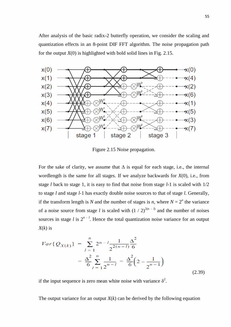
After analysis of the basic radix-2 butterfly operation, we consider the scaling and

quantization effects in an 8-point DIF FFT algorithm. The noise propagation path

for the output X(0) is highlighted with bold solid lines in Fig. 2.15.

Figure 2.15 Noise propagation.

For the sake of clarity, we assume that Δ is equal for each stage, i.e., the internal

wordlength is the same for all stages. If we analyze backwards for X(0), i.e., from

stage l back to stage 1, it is easy to find that noise from stage l-1 is scaled with 1/2

to stage l and stage l-1 has exactly double noise sources to that of stage l. Generally,

if the transform length is N and the number of stages is n, where N = 2n the variance

of a noise source from stage l is scaled with (1 / 2)2(n – l)

and the number of noises

sources in stage l is 2n – l

. Hence the total quantization noise variance for an output

X(k) is

(2.39)

if the input sequence is zero mean white noise with variance δ2.

The output variance for an output X(k) can be derived by the following equation

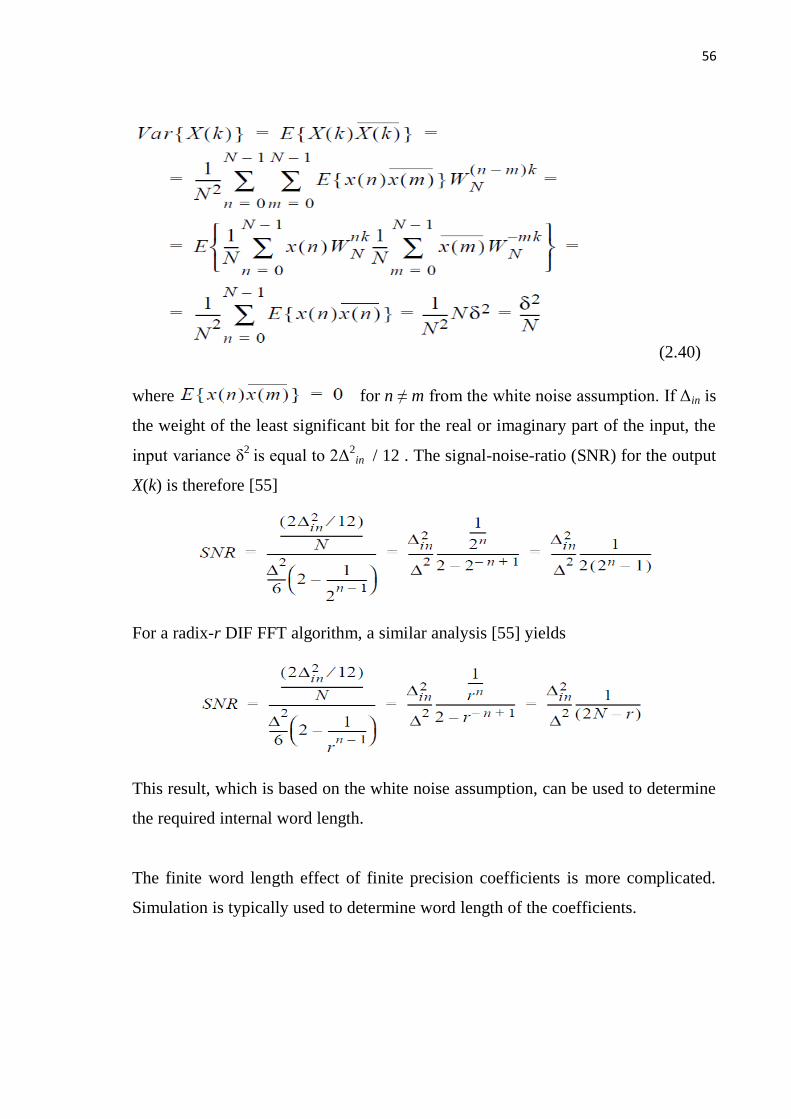
56

(2.40)

where for n ≠ m from the white noise assumption. If Δin is

the weight of the least significant bit for the real or imaginary part of the input, the

input variance δ2

is equal to 2Δ2

in / 12 . The signal-noise-ratio (SNR) for the output

X(k) is therefore [55]

For a radix-r DIF FFT algorithm, a similar analysis [55] yields

This result, which is based on the white noise assumption, can be used to determine

the required internal word length.

The finite word length effect of finite precision coefficients is more complicated.

Simulation is typically used to determine word length of the coefficients.

57

2.6.2 IDFT Implementation

An OFDM system requires both DFT and IDFT for signal processing. The IDFT

implementation is also critical for the OFDM system.

There are various approaches for the IDFT implementation. The straightforward

one is to compute the IDFT directly according to Eq. (1.2), which has a

computation complexity of O(N2). This approach is obviously not efficient.

The second approach is similar to FFT computation. If we ignore the scaling factor

1/N, the only difference between DFT and IDFT is the twiddle factor, which is

instead of . This can easily be performed by changing the read addresses of

the twiddle factor ROM(s) for the twiddle factor multiplications. It also requires the

reordering of input when a radix-r DFT is used. This approach adds an overhead to

each butterfly operation and change the access order of the coefficient ROM.

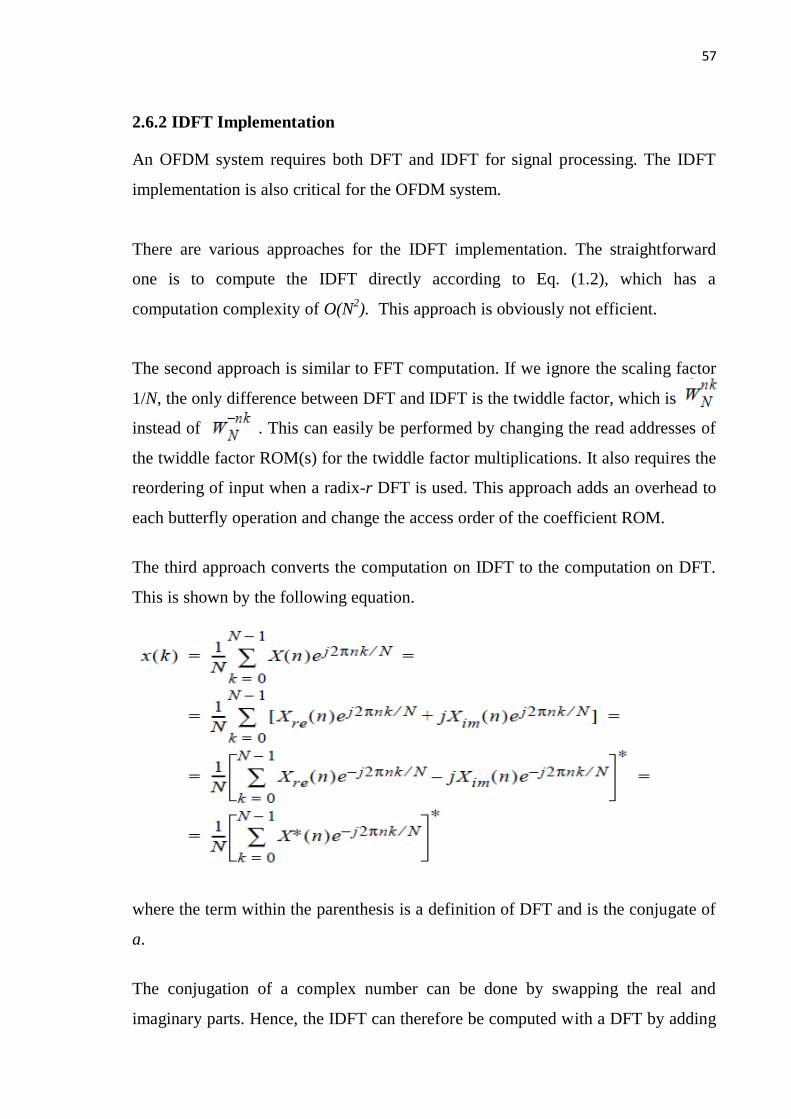
The third approach converts the computation on IDFT to the computation on DFT.

This is shown by the following equation.

where the term within the parenthesis is a definition of DFT and is the conjugate of

a.

The conjugation of a complex number can be done by swapping the real and

imaginary parts. Hence, the IDFT can therefore be computed with a DFT by adding

58

two swaps and one scaling: swap the real and imaginary part at input before the

DFT computation, swap the real and imaginary part at output from DFT, and a

scaling with factor 1/N.

2.7 Summary

This chapter provides the most commonly used FFT algorithms, e.g., the Cooley-

Tukey and Sande-Tukey algorithms. Each computation step was given in detail for

the Cooley-Tukey algorithms. Other algorithms like prime factor algorithm, split-

radix algorithm, and WFTA are also discussed. Then comparison of the different

algorithms in term of number of additions and multiplications are discussed.