processor architecture needed to handle fft algoarithm m. smith

Processor Architecture

Needed to handleFFT algoarithm

M. Smith

FFT algorithms There are more FFT algorithms performed

per day than any other algorithm in the world

Therefore, of course, custom parts of the processors to handle this situations

FFT Introduction, M. Smith, ECE, University of Calgary,

Canada

2

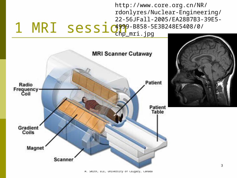
1 MRI session


Canada

3

http://www.core.org.cn/NR/rdonlyres/Nuclear-Engineering/22-56JFall-2005/EA28B7B3-39E5-4999-B858-5E3B248E5408/0/chp_mri.jpg

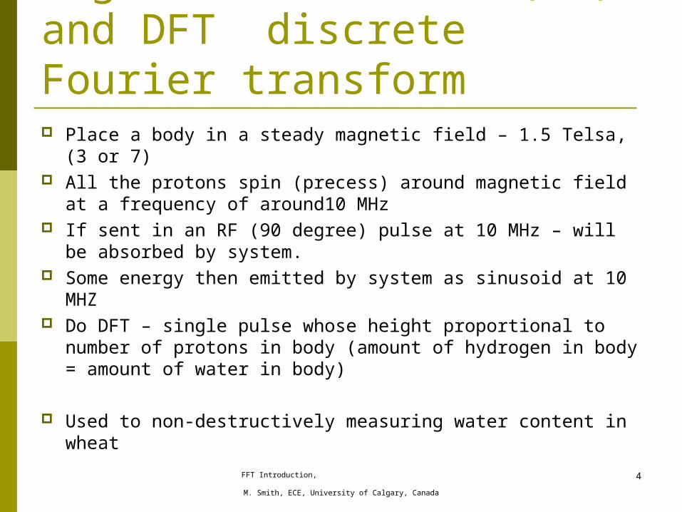
Magnetic resonance (MR) and DFT discrete Fourier transform Place a body in a steady magnetic field – 1.5 Telsa, (3 or 7) All the protons spin (precess) around magnetic field at a

frequency of around10 MHz If sent in an RF (90 degree) pulse at 10 MHz – will be

absorbed by system. Some energy then emitted by system as sinusoid at 10

MHZ Do DFT – single pulse whose height proportional to number

of protons in body (amount of hydrogen in body = amount of water in body)

Used to non-destructively measuring water content in wheat


Canada

4

Magnetic resonance imaging (MRI) and DFT discrete Fourier transform Place four bodies in a steady magnetic field – 1.5 Telsa, (3

or 7) Apply 90 pulse Apply DFT on response One signal at 10 MHz

Place four bodies in a steady magnetic field of 1.5 Telsa Apply 90 pulse Apply a “field gradient” in X direction Apply DFT on response Four signals 10 +G.X1, 10 + G.X2, 10 + G.X3 , 10 + G.X4

where Xi is the x position of object


Canada

5

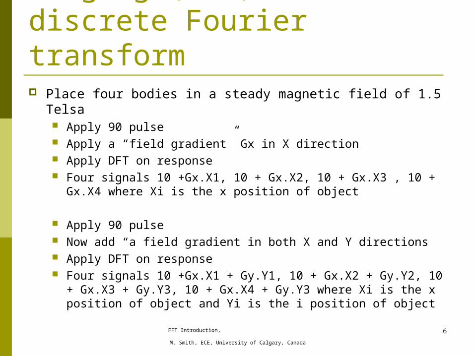
Magnetic resonance imaging (MRI) and DFT discrete Fourier transform Place four bodies in a steady magnetic field of 1.5 Telsa

Apply 90 pulse Apply a “field gradient” Gx in X direction Apply DFT on response Four signals 10 +Gx.X1, 10 + Gx.X2, 10 + Gx.X3 , 10 + Gx.X4

where Xi is the x position of object

Apply 90 pulse Now add “a field gradient in both X and Y directions Apply DFT on response Four signals 10 +Gx.X1 + Gy.Y1, 10 + Gx.X2 + Gy.Y2, 10 +

Gx.X3 + Gy.Y3, 10 + Gx.X4 + Gy.Y3 where Xi is the x position of object and Yi is the i position of object


Canada

6

1 MRI session Occurs for about 20 minutes Echo planar imaging (EPI)

Generates 19 2 D slices of the brain in about 60 seconds Each image is 256 pixels by 256

pixels x 19 Each image requires 256 * 256 * 19

DFTs / minute DFT is only ONE part of the

algorithm My research is using MRI for stroke

diagnosis


Canada

7

http://www.core.org.cn/NR/rdonlyres/Nuclear-Engineering/22-56JFall-2005/EA28B7B3-39E5-4999-B858-5E3B248E5408/0/chp_mri.jpg

http://www.magnet.fsu.edu/education/tutorials/magnetacademy/mri/images/mri-scanner.jpg

Tackled already this termThree types of DSP algorithms

Long loops, multiplication and addition intensive, regular (simple) memory accesses – e.g. 300 taps in FIR algorithms

Short loops involving multiplications and additions – e.g. 3 stages in IIR algorithms

DSP Introduction, M. Smith, ECE, University of Calgary,

Canada

8


Canada

9

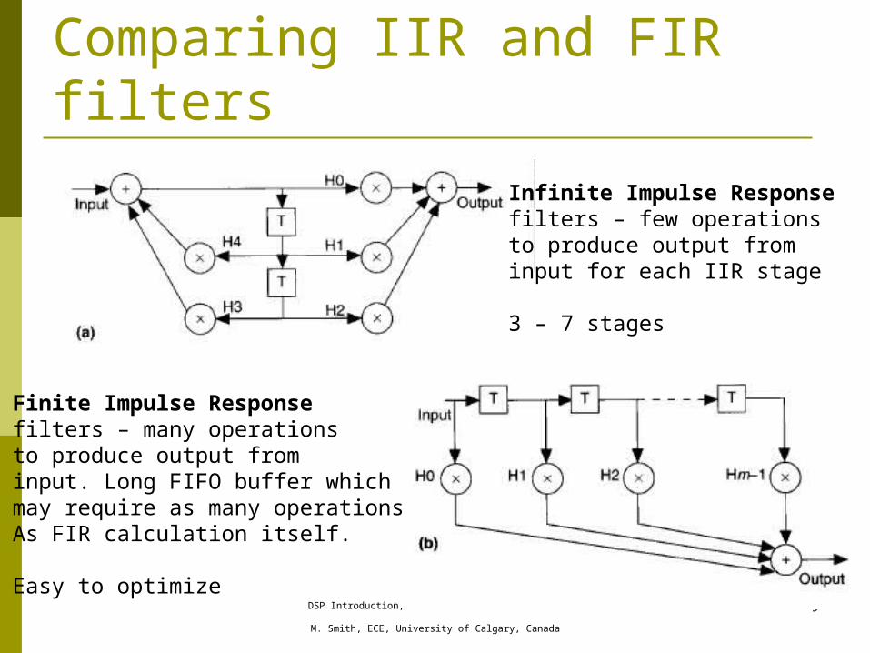
Comparing IIR and FIR filters

Infinite Impulse Responsefilters – few operations to produce output frominput for each IIR stage

3 – 7 stages

Finite Impulse Responsefilters – many operations to produce output frominput. Long FIFO buffer whichmay require as many operationsAs FIR calculation itself.

Easy to optimize

Discrete Fourier Transform FIR and IIR algorithms directly manipulate the

data in “the time domain”.

FIR -- Process M data points using N point FIR filter – involves M * (N-1) additions M * N multiplications M * N * 2 + M memory accesses Algorithm takes a time of Order (M * N)

Very slow if manipulating large amount of data


Canada

10

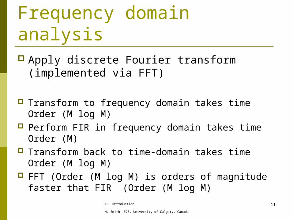
Frequency domain analysis Apply discrete Fourier transform

(implemented via FFT)

Transform to frequency domain takes time Order (M log M)

Perform FIR in frequency domain takes time Order (M)

Transform back to time-domain takes time Order (M log M)

FFT (Order (M log M) is orders of magnitude faster that FIR (Order (M log M)


Canada

11


Canada

12


Canada

13

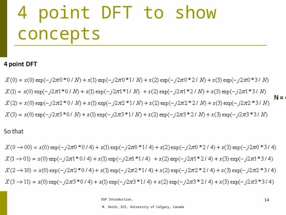
4 point DFT to show concepts


Canada

14

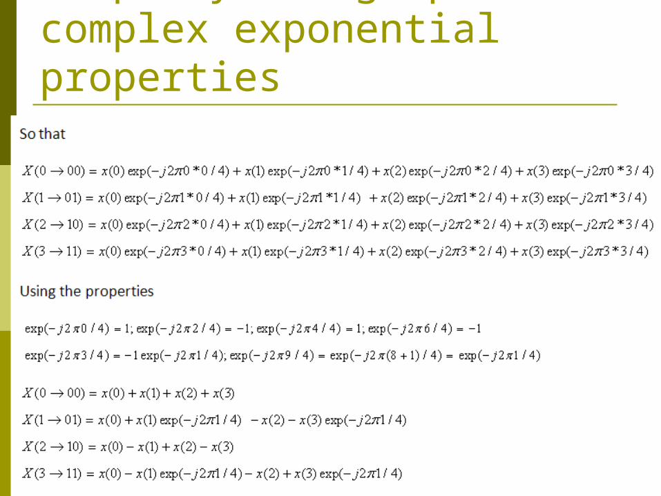
Simplify using special complex exponential properties


Canada

15

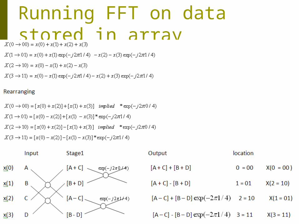
Running FFT on data stored in array


Canada

16

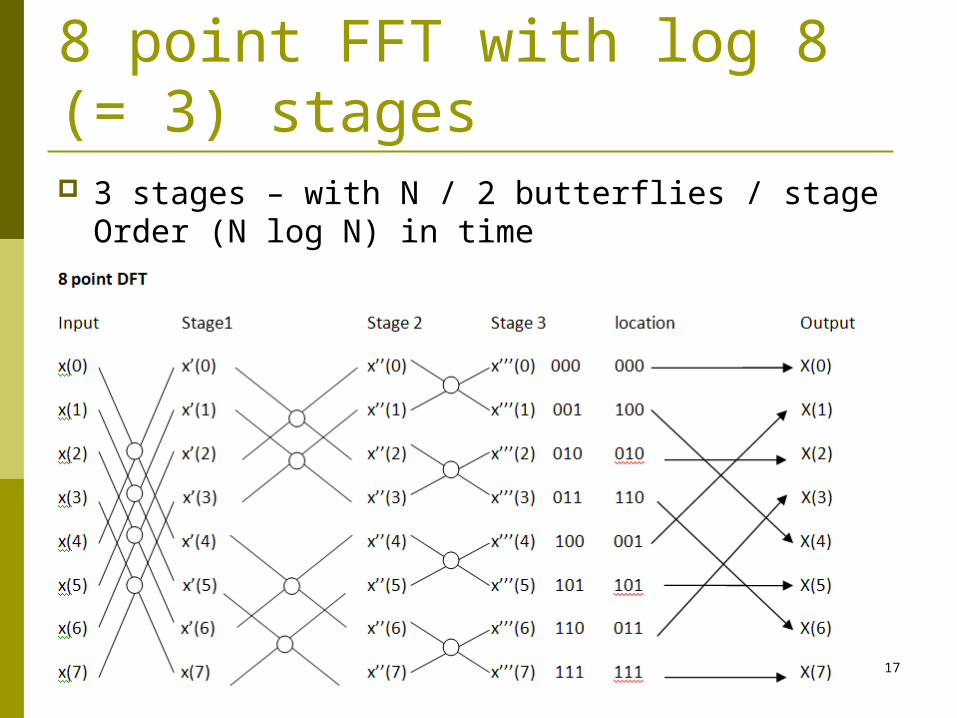
8 point FFT with log 8 (= 3) stages 3 stages – with N / 2 butterflies / stage

Order (N log N) in time


Canada

17

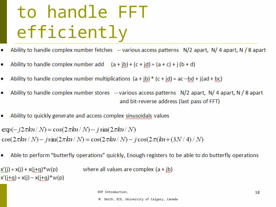
Architectural characteristics needed to handle FFT efficiently


Canada

18

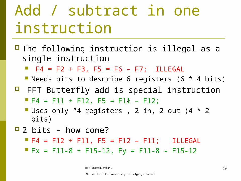
Add / subtract in one instruction The following instruction is illegal as a

single instruction F4 = F2 + F3, F5 = F6 – F7; ILLEGAL Needs bits to describe 6 registers (6 * 4 bits)

FFT Butterfly add is special instruction F4 = F11 + F12, F5 = F11 – F12; Uses only “4 registers”, 2 in, 2 out (4 * 2 bits)

2 bits – how come? F4 = F12 + F11, F5 = F12 – F11; ILLEGAL Fx = F11-8 + F15-12, Fy = F11-8 - F15-12


Canada

19

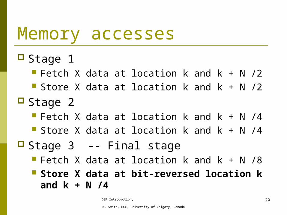
Memory accesses Stage 1

Fetch X data at location k and k + N /2 Store X data at location k and k + N /2

Stage 2 Fetch X data at location k and k + N /4 Store X data at location k and k + N /4

Stage 3 -- Final stage Fetch X data at location k and k + N /8 Store X data at bit-reversed location k

and k + N /4DSP Introduction,

M. Smith, ECE, University of Calgary, Canada

20

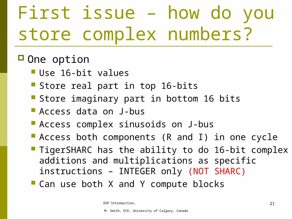
First issue – how do you store complex numbers? One option

Use 16-bit values Store real part in top 16-bits Store imaginary part in bottom 16 bits Access data on J-bus Access complex sinusoids on J-bus Access both components (R and I) in one cycle TigerSHARC has the ability to do 16-bit complex

additions and multiplications as specific instructions – INTEGER only (NOT SHARC)

Can use both X and Y compute blocksDSP Introduction,

M. Smith, ECE, University of Calgary, Canada

21

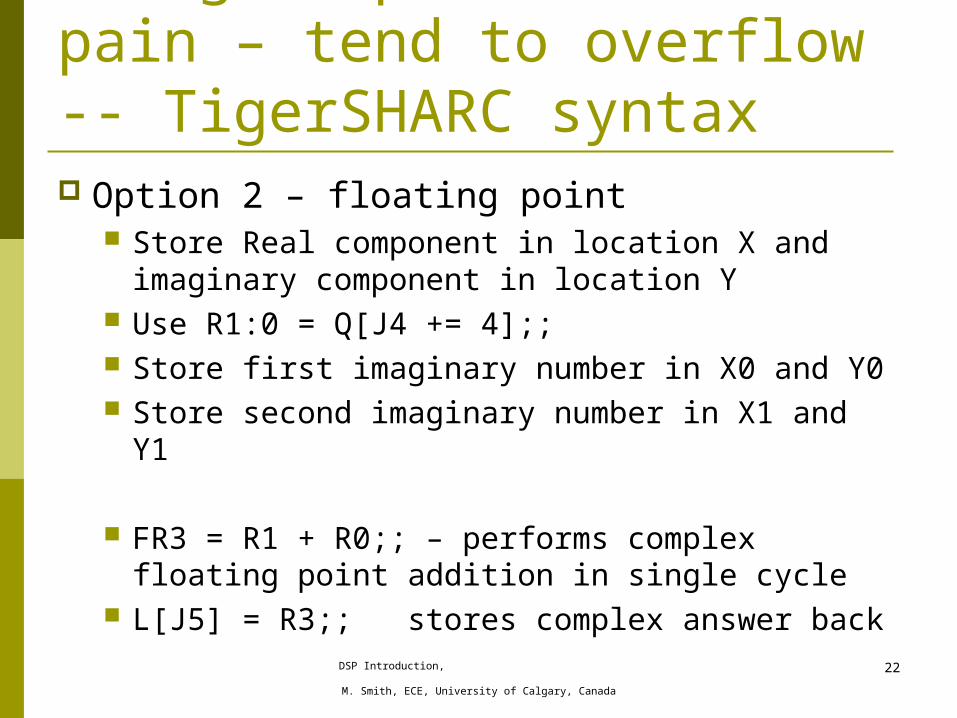
Integer operations a pain – tend to overflow -- TigerSHARC syntax Option 2 – floating point

Store Real component in location X and imaginary component in location Y

Use R1:0 = Q[J4 += 4];; Store first imaginary number in X0 and Y0 Store second imaginary number in X1 and Y1

FR3 = R1 + R0;; – performs complex floating point addition in single cycle

L[J5] = R3;; stores complex answer back


Canada

22

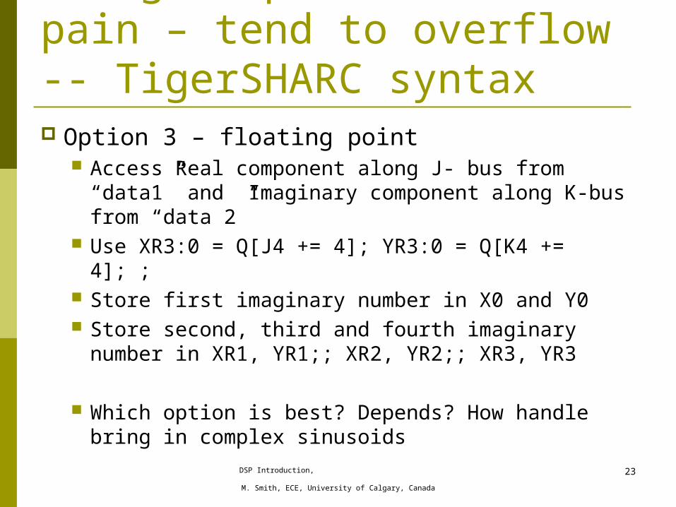
Integer operations a pain – tend to overflow -- TigerSHARC syntax Option 3 – floating point

Access Real component along J- bus from “data1” and Imaginary component along K-bus from “data 2”

Use XR3:0 = Q[J4 += 4]; YR3:0 = Q[K4 += 4]; ; Store first imaginary number in X0 and Y0 Store second, third and fourth imaginary

number in XR1, YR1;; XR2, YR2;; XR3, YR3

Which option is best? Depends? How handle bring in complex sinusoids


Canada

23

Bit reverse addressing


Canada

24

Bit reverse addressing – Check manual for “accurate details” before MII Only possible with I0, I1, I2? and I3? registers

(also I8, I9, I10?, I11?) You must start the array on a N aligned boundary

otherwise it does not work I0 = address pointer B0 = base register – point to start of array L0 = length of array register M0 = special circular buffer modify register ???? F4 = BR [I0 += 1]; // Correct SHARC syntax??? Bit-reverse addressing only works on POST-MODIFY

(permits next address to be calculated in parallel)


Canada

25

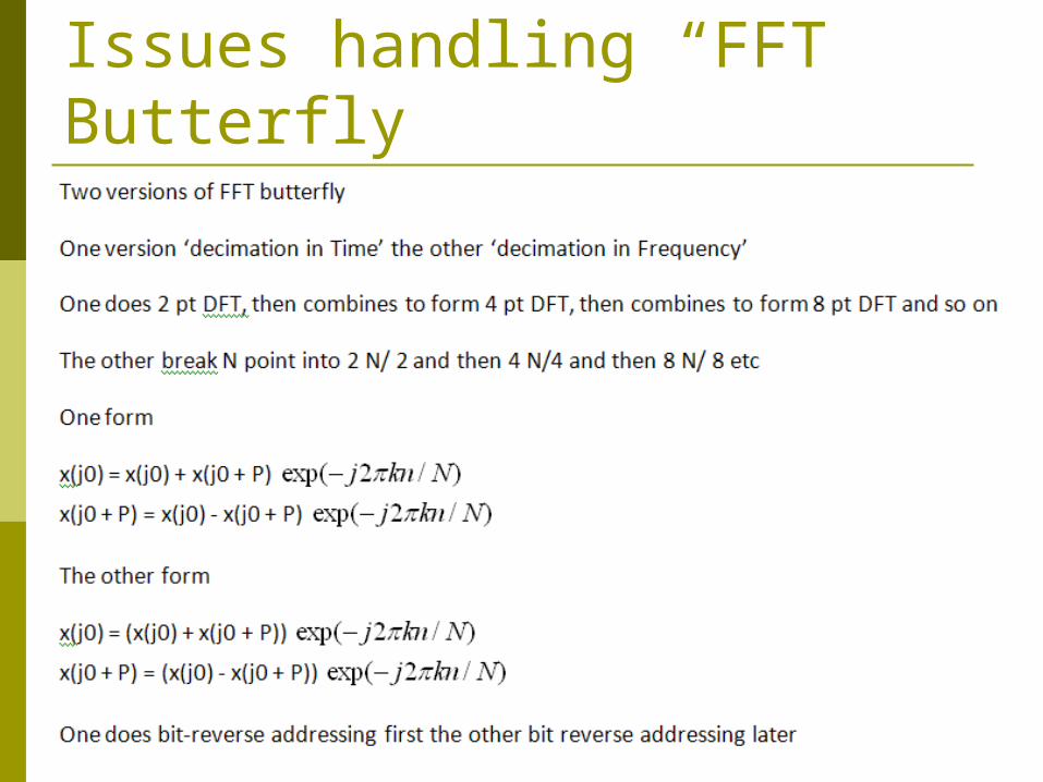
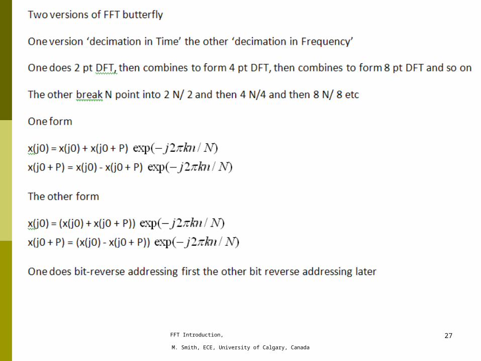
Issues handling “FFT Butterfly


Canada

26


Canada

27


Canada

28


Canada

29

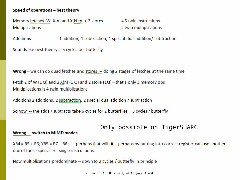
Only possible on TigerSHARC

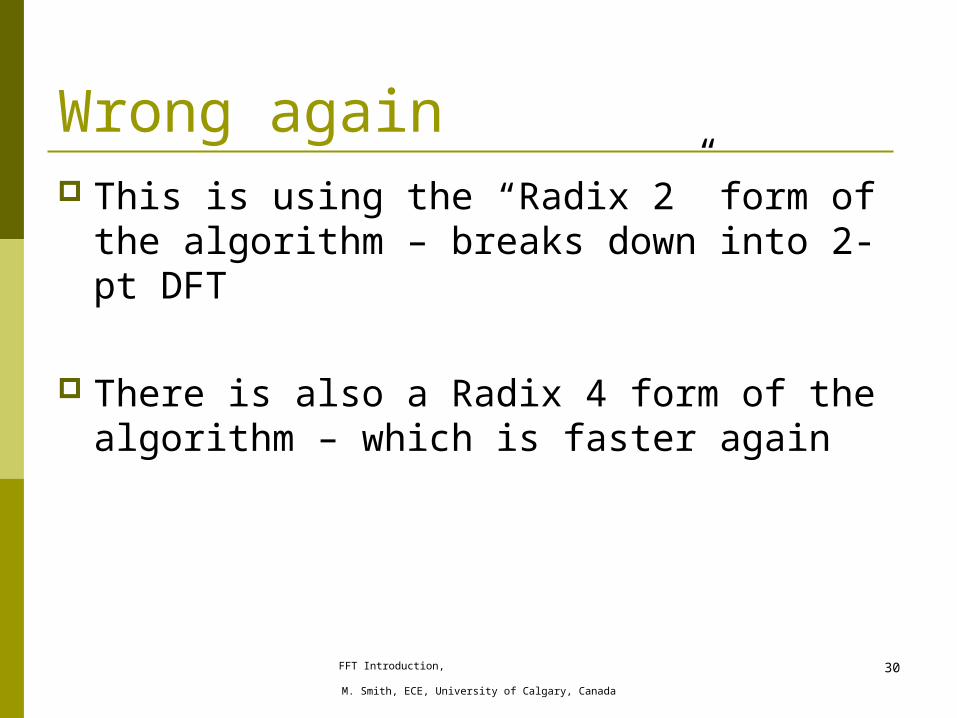
Wrong again This is using the “Radix 2” form of the

algorithm – breaks down into 2-pt DFT

There is also a Radix 4 form of the algorithm – which is faster again


Canada

30


Canada

31


Canada

32


Canada

33

TIGERSHARC

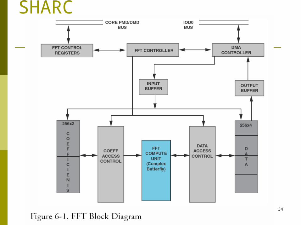
DSP Co-processor on SHARC


Canada

34


Canada

35

Will discuss FFT accelerator later

Was not available on previous SHARCS

Way to go with future processors Cheap processors + co-processors Cheap microcontroller + FPGA component


Canada

36

processor architecture needed to handle fft algoarithm m. smith

Documents