processing of dynamic wind pressure loads for …...processing of dynamic wind pressure loads for...

Wind and Structures, Vol. 21, No. 4 (2015) 425-442

DOI: http://dx.doi.org/10.12989/was.2015.21.4.425 425

Copyright © 2015 Techno-Press, Ltd.

http://www.techno-press.org/?journal=was&subpage=8 ISSN: 1226-6116 (Print), 1598-6225 (Online)

Processing of dynamic wind pressure loads for temporal simulations

Pascal Hémon

LadHyX, CNRS-Ecole Polytechnique, F-91128 Palaiseau, France

(Received November 7, 2014, Revised October 9, 2015, Accepted October 12, 2015)

Abstract. This paper discusses the processing of the wind loads measured in wind tunnel tests by means of multi-channel pressure scanners, in order to compute the response of 3D structures to atmospheric turbulence in the time domain. Data compression and the resulting computational savings are still a challenge in industrial contexts due to the multiple trial configurations during the construction stages. The advantage and robustness of the bi-orthogonal decomposition (BOD) is demonstrated through an example, a sail glass of the Fondation Louis Vuitton, independently from any tentative physical interpretation of the spatio-temporal decomposition terms. We show however that the energy criterion for the BOD has to be more rigorous than commonly admitted. We find a level of 99.95 % to be necessary in order to recover the extreme values of the loads. Moreover, frequency limitations of wind tunnel experiments are sometimes encountered in passing from the scaled model to the full scale structure. These can be alleviated using a spectral extension of the temporal function terms of the BOD.

Keywords: pressure loads; wind tunnel; wind gust; temporal simulation; bi-orthogonal decomposition

1. Introduction

In the field of wind-excited civil engineering structures, temporal simulations are increasingly

important, due to the larger size of the structures and to their shape becoming more and more

complex. Nowadays the main practical difficulty for designers is to harness the structure against

the effects of atmospheric turbulence. A complex structure under construction is particularly

delicate and sensitive to turbulent gusts. As a consequence, there is a need for more accurate

computations which can account for the nonlinear behavior of the structure and the combination

with other kinds of loads.

The classical techniques for solving the dynamical problem are generally based on spectral

methods, combined with probabilistic features in order to estimate the maxima of displacement.

Certain types of nonlinear behavior cannot be adequately captured with such techniques. Temporal

simulations do not suffer from such limitations, as long as the simulation length is statistically

pertinent. In addition they allow direct coupling with other phenomena such as the excitation due

to passing vehicles. Moreover, from a structural computation point of view, one can avoid

quadratic recombination of the eigenmode response, so that temporal simulations can provide

Corresponding author, Ph.D., E-mail: [email protected]

Pascal Hémon

better maxima structural stress estimations.

We consider in this study the case of a structure with a complex 3D shape which could be a

stadium roof, for instance, or a glass sail as the one shown further. The temporal simulation of the

response to wind excitation is solved in a classical manner using the structure eigenmodes

superposition, as suggested by Géradin and Rixen (1997). The displacement solution 𝑋(𝑡) of the

equation of motion,

�̈� �̇� 𝑋 (𝑡) (1)

is then expressed as a linear combination of the eigenvectors Wi, as written in Eq. (2). M is the

mass matrix, C the damping matrix and K the stiffness matrix. (𝑡) is the time-dependant

external wind excitation.

𝑋(𝑡) ∑ (𝑡) 𝑚 (2)

Due to the orthogonality of eigenvectors as in the relations Eq. (3), where 𝜔 are the eigen

angular frequencies, and 𝛿 ,𝑗 the Kronecker symbol

( , 𝑗) 𝛿 ,𝑗 ; ( , 𝑗) 𝜔 𝛿 ,𝑗 (3)

one obtains the final system Eq. (4) of m scalar equations. These are solved numerically in time, in

order to determine the general coordinates (𝑡). The reduced damping of each eigenmodes is

denoted 𝜂 .

{ ̈ (𝑡) 𝜂 𝜔 ̇ (𝑡) 𝜔

(𝑡) ( (𝑡), ) ,

(4)

In this method, as pointed out by Géradin, the number of eigenmodes m has to be large enough,

representing a sufficient amount of the total mass in each direction of space. Also, the frequency

range of retained eigenmodes should cover the frequency range of the external excitation. This

excitation is supposed here to have been measured in a wind tunnel, such that it provides the time

series of wind pressure on each node of the structural mesh.

This method is widely used in industrial contexts, problems arise however in the computational

cost of evaluating m scalar products ( (𝑡), ) at each time step. The present paper proposes to

use a data compression technique which helps to reduce this cost, and, in a second step, a method

to improve quality of numerical results when the frequency content of aerodynamic tests does not

match the one of the structure. To illustrate the proposed method, we use an example, a large glass

roof, which is thoroughly analyzed from a structural design perspective.

2. Data compression technique

2.1 Proper orthogonal decomposition method

A number of techniques are available for the analysis and compression of fluctuating data such

as wall pressure. Of particular interest is the Proper Orthogonal Decomposition (POD) and its

numerous variations (Singular Value Decomposition, Principal Component Analysis,

Karhunen-Loève Decomposition) that cover almost the same process (Liang et al. 2002).

These techniques perform a decomposition of the pressure signal onto a basis of orthogonal

426


spatial eigenfunctions or modes. These spatial functions are the eigenvectors of the spatial

cross-correlation matrix of the signal. The corresponding time functions are the Principal

Components. They are computed a posteriori by projection of the spatial functions on the original

signal.

Armitt (1968) was probably the first who used this method in wind engineering studies. In 2007,

an extensive review of the use of POD in different scientific fields close to wind engineering was

published (Solari et al. 2007). It pointed out the different names cited above, and that Singular

Value Decomposition is probably the first version of this tool which appeared. Recently Andrianne

(2013) used the Common-base POD (CPOD) introduced by (Kriegseis et al. 2010) in order to

analyze the flow field around a moving rectangular prism. The principle of CPOD is to use several

datasets corresponding to different values of a parameter of the system, such as the wind velocity.

The spatial functions are then representative of the problem for every value of the parameter

included in the range of the dataset.

In POD, the number of terms in the decomposition is optimized so as to represent the

maximum of the signal energy with the minimum number of terms (Holmes et al. 1996). This

optimization process leads to the result that the eigenvectors of the spatial cross-correlation matrix

are the optimal choice. Efficient signal compression is then performed. To be mathematically

rigorous, POD requires that the pressure signal is square-integrable, ergodic, stationary and

Gaussian. However, it is generally used even when these conditions are not completely satisfied.

As discussed in (Tamura et al. 1999) POD is more efficient when the signal is centred, i.e., when

the temporal mean has been substracted from the original signals. The analogy of POD “modes”

with structural eigenmodes was studied in (Feeny and Kappagantu 1998).

For flows around simple structure shapes, it is often possible to physically interpret the

eigenfunctions and to link them to a physical phenomenon such as vortex shedding (Ricciardelli

2005). Nevertheless, the physical character of individual modes can be obscured by the constraint

of orthogonality of eigenfunctions (Holmes et al. 1997, Carassale 2001). For complex 3D

structures, physical interpretation of eigenfunctions is usually no longer possible and POD is

therefore interesting only for data compression.

In the snapshot POD introduced in (Breuer and Sirovitch 1991), the space is replaced by time,

such that the POD terms represent a basis of temporal eigenfunctions which are simply the

eigenvectors of the temporal cross-correlation matrix. The purpose is mainly to reduce the size of

the eigenvalue problem when the number of time steps is smaller than the number of nodes, which

often occurs in the analysis of computational results.

2.2 Bi-orthogonal decomposition

In this paper we use a different, but very similar technique called bi-orthogonal decomposition

(BOD), which was first introduced in (Aubry et al. 1991) where all mathematical details and

demonstrations can be found. Physicists used this technique in order to characterize the coherent

structures in plasma turbulence, for which the tool proved to be very efficient (Benkadda et al.

1994). BOD was also used for travelling wave detection in plant biomechanics (Py et al. 2005) and

computational data analysis in (Dupont et al. 2010). Its application to the pressure distribution on

simple shapes, static or moving, was discussed in (Hémon and Santi 2003).

In BOD, the assumptions about the original signal are reduced to square-integrability only. Its

use therefore will be more rigorously justified in the current application than POD, since ergodic,

Gaussian and stationary pressure signals are not required. It will be shown in particular that the

427

Pascal Hémon

signals at hand are indeed not Gaussian. BOD is a suitable technique even in cases when the signal

contains intermittent events, as pointed out in (Py et al. 2005). Such events are simply extracted as

individual spatio-temporal structures.

BOD can be considered as a simultaneous mixing between POD and snapshot POD, where the

spatial eigenfunctions Ψ𝑘 are called topos, and the temporal eigenfunctions 𝜑𝑘(𝑡) are named

chronos. The decomposition consists in writing the pressure distribution as a linear combination of

these functions, which are normalized by a factor 𝛽𝑘, representing the individual energy of each

spatio-temporal structure (i.e., a topos and a chronos of same rank k)

(𝑡) ∑ 𝛽𝑘 𝜑𝑘(𝑡) Ψ𝑘𝑛𝑘 (5)

The topos and the chronos form orthogonal sets , such that

(Ψ𝑘 , Ψ𝑙) 𝛿𝑘,𝑙 ; (𝜑𝑘 , 𝜑𝑙) 𝛿𝑘,𝑙 (6)

As in POD, the topos are the eigenvectors of the spatial cross-correlation matrix, while

simultaneously the chronos are the eigenvectors of the temporal cross-correlation matrix. But an

important feature of BOD is that the topos and the chronos are intrinsically linked, by a common

eigenvalue √𝛽𝑘. This is the main difference between POD and BOD.

For this reason, the non-zero mean value of the signal has to be preserved in BOD, because it is

not possible to simultaneously remove both the temporal and the spatial average. If the mean value

in time is substracted, as in classical POD, the decomposition leads to centred chronos, but the

topos computed in such a case would be compromised. Conversely, it is not possible to extract the

spatial mean from the topos without perturbing the chronos. In other words, if ̅ is the mean

value in time and ⟨ ⟩ the mean value in space, the BOD of (𝑡) − ̅ is different from the

decomposition of (𝑡) − ⟨ ⟩ , so that it is not possible to choose between one of these corrected

signals. A mathematical demonstration of this point can be found in (Aubry et al. 1991) and a

discussion concerning wall pressures is given in (Hémon and Santi 2003), especially when

heterogeneous mean values in time are present.

The topos are often called “modes” by authors who use classical POD, for instance (Kho et al.

2002). These authors used an ARMA technique to recover the time functions, which in the present

formalism are replaced by the chronos. In the present paper we will keep the name topos for the

spatial function of the BOD and reserve the term “mode” for the structural eigenmodes.

In BOD, the decomposition is not constructed to be optimal, as it is explicitly the case for POD.

Aubry et al. (1991) describe the technique as a “deterministic tool rather than statistical”. But in

practice it is very efficient in the sense that few terms are found necessary in order to reach an

energy close to the total energy of the original signal expressed by

∑ 𝛽𝑘 ( , )𝑘 (7)

If N is the total number of nodes and T the number of time steps, the BOD will then retain only

n terms with the hope that n << min(N, T) for the efficiency of the signal compression. In what

follows, the energy of each decomposition term is reduced by reference to this total energy and is

expressed as a percentage.

In order to use the decomposition in equations Eq. (4), one has to transform the pressure

vectors (𝑡) of size N into a three-component force vector (𝑡) of size 3N

(𝑡) (𝑡) (8)

428


where is the 3N-component vector constructed with all the nodal vectors normal to the surface,

normalized by their surface in square meters. This standard operation is performed within the finite

element code used for the structural computation.

Combination of the decomposition Eq. (5) with relation Eq. (8) yields the modified topos as

Ψ 𝑘 Ψ𝑘 (9)

The equation of motion (4) leads then to the final system

{ ̈ (𝑡) 𝜂 𝜔 ̇ (𝑡) 𝜔

(𝑡) ∑ 𝛽𝑘 𝜑𝑘(𝑡) 𝑛𝑘 (Ψ 𝑘 , )

, (10)

In this new formulation, the m × n scalar products (Ψ 𝑘, ) do not depend on time, and they

must be computed only once as initial constants of the temporal simulation. The computation time

is thereby considerably reduced; it can be simply estimated by comparing the cost of m × n scalar

products to the cost of m × T products. The computational gain is finally proportional to the ratio

of time steps T and the number of terms n retained in the BOD. This gain is all the more

pronounced as the simulated time interval in longer.

3. Application example: a glass sail

3.1 Presentation of the case study and its aerodynamic data

The glass sail used to illustrate the method is a ∧ type which stands at 53 m of height above

the ground. It is part of a large new building, the “Fondation Louis Vuitton” near Paris which can

be seen in Fig. 1. It includes 12 huge glass sails and the chosen one is studied here in its final

environment. Its surface is about 750 m2 and its total mass about 210 t. It is supported on a

concrete structure by means of a series of metal beams, which make this sail an almost

independent and deformable sub-structure. The modal analysis of the glass sail alone, which is

used in this paper, assumes that the concrete structure is rigid which is reinforced with the large

rigidity of the beams that link the sail to the concrete. A modal analysis yields 20 eigenmodes in

the frequency range [2.50 – 4.99 Hz], representing around 60, 70 and 80% of the total mass in

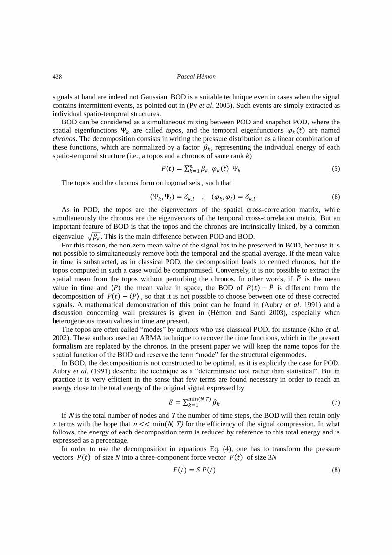
each direction X, Y and Z, respectively. Fig. 2 shows the first eigenmode at 2.50 Hz and gives a

view of the shape of the glass sail.

When the concrete structure is taken into account, the first eigenfrequency of the glass sail

decreases to 2.23 Hz (instead of 2.50 Hz), showing that the flexibility of the concrete, neglected in

this paper, is indeed small. This assumption was confirmed once again in the end of the study,

since the maximum displacement of the witness node was found larger of only 5% with the

complete structure, by comparison of the result obtained with the glass sail alone.

Aerodynamic data were obtained in the boundary layer wind tunnel of CSTB in Nantes on a

model of the entire building at a scale 1/125 shown Fig. 3. The atmospheric boundary layer is

simulated by means of rugosity devices mounted upstream of the test section. Its characteristics

follow those of the construction site in relation with Eurocode and its French appendix. The

simulated boundary layer is of the type IV (suburban area) with a rugosity lenght of 1 m. Different

wind directions were completely explored, but we use here only the direction which generates the

largest excitation on the glass sail. Pressure taps were flush mounted on the glass surface and

connected to pressure transducers inside the model by tubes of minimized length. The reference

429

Pascal Hémon

pressure is connected to the static pressure obtained on the reference Pitot tube of the wind tunnel.

The acquisition of all channels is considered to be synchronized in the frequency range up to 100

Hz. This kind of wind tunnel measurements is increasingly used in civil engineering applications,

such as in (Deng et al. 2015) for instance.

The structural mesh contains 421 nodes loaded by the wind, while a few more are used for the

structural computation. The number and the position of these nodes do not correspond exactly to

the pressure taps mounted on the model, so that an interpolation procedure within the finite

element code was used in order to obtain pressure signals acquired on the model on the nodes of

the structural mesh.

In what follows, all reported data values pertain to the full scale configuration. The reference

velocity at 10 meters high is 26 m/s. Measurements were recorded over 2 hours in total, divided

into 12 sequences of 10 minutes each. The rescaled sampling frequency was 2.6 Hz (which is the

result of the scale effect, the measurement sampling frequency and the reference velocity).

Fig. 1 The “Fondation Louis Vuitton” in Paris

430


Fig. 2 First eigen mode of the glass sail at 2.50 Hz, colored by displacement magnitude

Fig. 3 The wind tunnel model of the Fondation Louis Vuitton, at scale 1/125

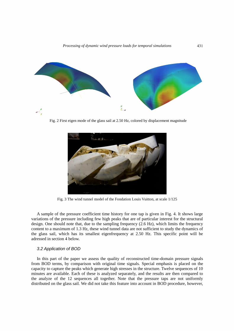
A sample of the pressure coefficient time history for one tap is given in Fig. 4. It shows large

variations of the pressure including few high peaks that are of particular interest for the structural

design. One should note that, due to the sampling frequency (2.6 Hz), which limits the frequency

content to a maximum of 1.3 Hz, these wind tunnel data are not sufficient to study the dynamics of

the glass sail, which has its smallest eigenfrequency at 2.50 Hz. This specific point will be

adressed in section 4 below.

3.2 Application of BOD

In this part of the paper we assess the quality of reconstructed time-domain pressure signals

from BOD terms, by comparison with original time signals. Special emphasis is placed on the

capacity to capture the peaks which generate high stresses in the structure. Twelve sequences of 10

minutes are available. Each of these is analyzed separately, and the results are then compared to

the analyze of the 12 sequences all together. Note that the pressure taps are not uniformly

distributed on the glass sail. We did not take this feature into account in BOD procedure, however,

431

Pascal Hémon

this can be done by using a method similar the one suggested in (Jeong et al. 2000).

The first topos is closely related to the temporal mean, and a comparison between these two is

shown in Fig. 5 for pressure signals of the first sequence. Note that a direct comparison of their

absolute values is meaningless, as the topos is normalized differently.

Second and interesting result is the fact that all sequences provide the same topos, at least for

the first fifteen terms that have been analyzed in detail. In Fig. 6 the topos 2 to 5 of a single

sequence are plotted. This is confirm with the help of the Modal Assurance Criterion (Pastor et al.

2012) which is an indicator that can be seen as a coherence value between two mode shapes. Value

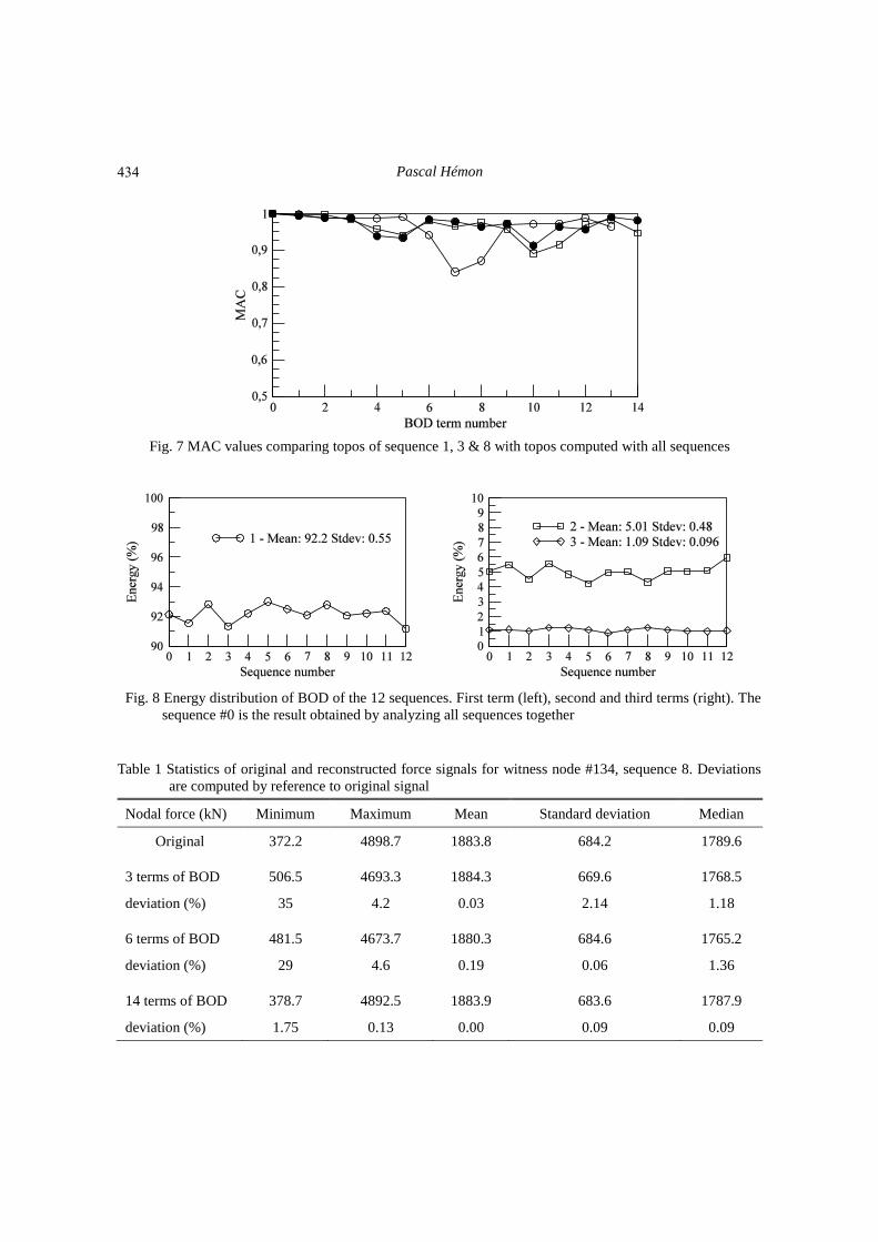
close to 1 means that the compared vectors are consistent. In Fig. 7 we present the MAC value for

the topos of 3 sequences referred to the topos computed with all sequences together. Values are

most of the time upper 0.9 and in the range [0.8-0.9] in very few cases. This implies that the

technique is robust in the sense that the analysis of 10 minutes of pressure records yields to the

same results as an analysis of 2 hours.

Fig. 4 Sample of signal from an individual pressure tap

Fig. 5 Comparison of the first topos of sequence 1 (left) with the mean pressure distribution of the same

sequence (right). The color map is adjusted between min and max values of each data set

432


Fig. 6 Topos #2 to 5 of sequence 1

This robustness is confirmed by an examination of the energy distribution along the terms of

BOD. In Fig. 8, the energy of the first three spatio-temporal structures is plotted for each 12

sequences and for all of them together, referenced as #0. We observe a relatively constant energy

distribution for each rank. This point is again confirmed by Fig. 9, where the energy distribution of

BOD terms of individual sequences is found to be very close to that obtained from all sequences.

Usually one considers that the signal is properly reconstructed when the cumulated energy in

the terms retained in the BOD is closest to that of the maximum. In practice, one has to make a

choice, for instance 95% is commonly admitted by experience (Hémon and Santi 2007), because it

has been found sufficient to fit with the mean and the RMS values. In fact, the present results show

that the amount of energy has to be much closer to its maximum in order to accurately capture the

extreme values of the signal.

Table 1 presents the statistical data for a witness node of sequence 8. The absolute deviation of

the statistical characteristics of the reconstructed signals are given relative to the original signal.

The cumulated energy amount is 98.33% with 3 BOD terms, 99.398% with 6 terms and 99.957%

with 14 terms. The mean value is rapidly reached since it is mainly represented by the first BOD

term, as shown before. However only the latter case with 14 terms leads to an acceptable

representation of the signal extrema, although the standard deviation is well represented more

easily with only 6 terms. These data, among others not shown here, bring us to conclude that a

minimum amount of 99.95 % of energy is required in such an application.

433

Pascal Hémon

Fig. 7 MAC values comparing topos of sequence 1, 3 & 8 with topos computed with all sequences

Fig. 8 Energy distribution of BOD of the 12 sequences. First term (left), second and third terms (right). The

sequence #0 is the result obtained by analyzing all sequences together

Table 1 Statistics of original and reconstructed force signals for witness node #134, sequence 8. Deviations

are computed by reference to original signal

Nodal force (kN) Minimum Maximum Mean Standard deviation Median

Original 372.2 4898.7 1883.8 684.2 1789.6

3 terms of BOD 506.5 4693.3 1884.3 669.6 1768.5

deviation (%) 35 4.2 0.03 2.14 1.18

6 terms of BOD 481.5 4673.7 1880.3 684.6 1765.2

deviation (%) 29 4.6 0.19 0.06 1.36

14 terms of BOD 378.7 4892.5 1883.9 683.6 1787.9

deviation (%) 1.75 0.13 0.00 0.09 0.09

434


Fig. 9 Energy of the BOD terms. Cumulative value is always greater than 99.95% with 14 terms, in any

individual sequences and for all of them together

Fig. 10 Probability density functions obtained with time history of wind load on witness node #134 in

sequence 8

The non Gaussian character of these signals is shown by the difference between the mean

values and the median that appears in the Table 1. It can be visualized more clearly with

Probability Density Functions (PDF), presented in Fig. 11. The positive skewness is clearly visible.

It shows again that the reconstruction by BOD is correct with 14 terms, at which point more than

99.95% of the signal energy is recovered.

435

Pascal Hémon

Fig. 11 Power spectral densities of three generalized forces among 20, showing the linear extrapolation up

to 5 Hz

4. Time domain simulation and frequency content adjustment

As already mentioned, the time domain simulation cannot be performed directly in this specific

application because of the disagreement between the frequency band covered by the wind tunnel

tests and the eigenfrequencies of the structure. The objective of this chapter is to present the

methods that can be used to compensate for this issue. Of course the scientific rigor would lead to

another wind tunnel test campaign that could adequately fit with the need. But in an industrial

context, this is not always possible, due to delays or costs: one may encounter such a situation.

Concretely, the problem is to extrapolate the frequency band of the pressure signals from [0 –

1.25 Hz] to the one of the eigenmodes, up to 5 Hz. Then one has to enrich the signals between 1.25

and 5 Hz. Before that we make the verification that for the range of frequency just below the one

which is concerned by extrapolation, the spatial correlation is small. This is due to the environment

of the structure, and the structure itself, that generate a highly turbulent flow. Combined with the

fact that the frequency is relatively high, the spatial correlation is not taken into account in the

extrapolation procedure.

In the following we will compare two techniques: the first one applies to the classical time

simulation, given by Eq. (4), in which the aerodynamic loads are used in the form of generalized

forces 𝑓 (𝑡) ( (𝑡), ). The second technique applies to the time simulation using compressed

aerodynamic pressure by BOD, as in Eq. (10), in which the time history of the aerodynamic loads

is provided by the chronos 𝜑𝑘(𝑡).

4.1 The modal superposition method

Enriching the signals up to 5 Hz means that one has to oversample the time series four times.

However, the method of enrichment is physically possible in the frequency domain. The procedure

needs then to perform a round trip to the frequency domain.

The method can be summarized in three main points:

436


i. compute the power spectral densities (PSD) of the generalized forces. The Fourier

transform of 𝑓 (𝑡) is computed (via a Fast Fourier Transform algorithm), to obtain a

modulus |𝑓 (𝜔)| and a phase 𝜃( 𝑓 (𝜔)). The PSD is approximated by the modulus

square |𝑓 (𝜔)| .

ii. enrich the PSD by linear extrapolation up to 5 Hz (in a log-log space), giving the new PSD

|𝑔 (𝜔)| .

iii. come back to the time domain by means of an inverse Fourier transform. The modulus

|𝑔 (𝜔)| and the phase 𝜃( 𝑓 (𝜔)) computed in (i) are the input to this inverse Fourier

transform.

The validation of steps (i) and (iii) was easily performed by comparing a signal issued from this

process, without enrichment, to the original one. While these steps are standard operations, using

complex Fast Fourier Transform tools, the second step requires more explanation and justification.

To illustrate the idea, Fig. 11 presents the PSD of some randomly chosen generalized forces.

The shapes of the curves are similar to that of a wind spectrum (Crémona and Foucriat 2002): for

low frequencies one observes a flat region which progressively evolves into a straight decreasing

line. The linear extrapolation is based on the tail region of the original PSD, where this monotonic

decrease with a more or less constant slope occurs. By experience, it is reasonable to enrich the

PSD using this kind of extrapolation; however, it makes the assumption that a coupling “resonant”

phenomenon, such as a vortex shedding excitation, does not exist in this extended frequency range.

Considering the shape of the current structure, this assumption is justified.

In this particular case, the truncated range [0.3 – 0.8 Hz] was used to compute the linear

extrapolation. Indeed, it was detected that the extreme tails of the original PSD were perturbed by

an aliasing error issued from the measurement system. So the range of the curve used as the basis

for the extrapolation was truncated by removing the band [0.8 – 1.25 Hz].

Starting from these PSD, the time signal, oversampled and enriched, is obtained by using a

complex inverse Fourier transform. It serves then as the excitation term in order to solve

numerically Eq. (4). The standard Newmark method is used.

In Fig. 12, an example of time history is presented, comparing the solution obtained from the

original signal with the solution obtained from the processed one. Both are very similar because

the enriched part of the excitation has a frequency range where the unsteady forces are relatively

small. The main excitation of the structure results in fact from the low frequency range which was

already captured by the wind tunnel measurements. Therefore the enrichment of the signal is a

small correction of wind tunnel measurements.

4.2 The BOD method

In this case, the temporal part of the excitation in Eq. (10) is given by the chronos 𝜑𝑘(𝑡). Similarly to the previous method, the extrapolation is performed on the PSD of the chronos

directly, as illustrated in Fig. 13. The behavior of this extension is slightly different than in the

modal method, because the evolution of the PSD of the chronos with their rank is increasingly flat.

This leads to an increasingly horizontal extrapolation line, whereas for the modal method the

extrapolations were quite similar in all cases.

Once the enriched PSD are computed, the inverse Fourier transformation to the time domain is

performed in the same way as for the generalized forces. Then the time simulation of Eq. (10) can

437

Pascal Hémon

be performed using the Newmark method.

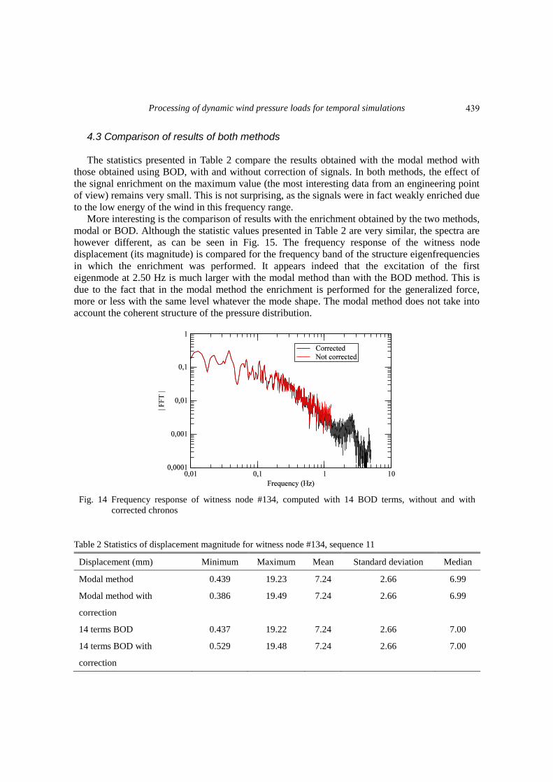
The comparison of the response of the witness node #134 with and without correction is shown

in Fig. 14 in the frequency domain. Obviously, the enriched spectrum has an extended range in

frequency and we can observe for instance a peak around 2.5 Hz that corresponds to the excitation

of the first eigenmode of the glass roof. However, this peak remains of small amplitude since the

unsteady wind loads are small in this range of frequency.

Fig. 12 Witness node displacement computed with modal superposition method, without and with

frequency extension

Fig. 13 Power spectral densities of four chronos among 14, showing the linear extrapolation up to 5 Hz

438


4.3 Comparison of results of both methods

The statistics presented in Table 2 compare the results obtained with the modal method with

those obtained using BOD, with and without correction of signals. In both methods, the effect of

the signal enrichment on the maximum value (the most interesting data from an engineering point

of view) remains very small. This is not surprising, as the signals were in fact weakly enriched due

to the low energy of the wind in this frequency range.

More interesting is the comparison of results with the enrichment obtained by the two methods,

modal or BOD. Although the statistic values presented in Table 2 are very similar, the spectra are

however different, as can be seen in Fig. 15. The frequency response of the witness node

displacement (its magnitude) is compared for the frequency band of the structure eigenfrequencies

in which the enrichment was performed. It appears indeed that the excitation of the first

eigenmode at 2.50 Hz is much larger with the modal method than with the BOD method. This is

due to the fact that in the modal method the enrichment is performed for the generalized force,

more or less with the same level whatever the mode shape. The modal method does not take into

account the coherent structure of the pressure distribution.

Fig. 14 Frequency response of witness node #134, computed with 14 BOD terms, without and with

corrected chronos

Table 2 Statistics of displacement magnitude for witness node #134, sequence 11

Displacement (mm) Minimum Maximum Mean Standard deviation Median

Modal method 0.439 19.23 7.24 2.66 6.99

Modal method with

correction

0.386 19.49 7.24 2.66 6.99

14 terms BOD 0.437 19.22 7.24 2.66 7.00

14 terms BOD with

correction

0.529 19.48 7.24 2.66 7.00

439

Pascal Hémon

Fig. 15 Frequency response of witness node #134, computed with the enriched signals. Comparison of

modal method with BOD method. Structural frequencies are shown with vertical bars

This is not the case in the BOD method because it is performed directly by means of the scalar

product (Ψ 𝑘, ), appearing in Eq. (10), which combines the topos with the mode shapes. In this

case, it is physically obvious that a coherent structure of the pressure load, represented by a topos,

leads to an eigenmode excitation only if their respective “shapes” are close. This physical property

seems better represented in the BOD method where the requested enrichment of the temporal part

of the pressure signals is performed on the chronos, which reflects exactly the temporal evolution

of the coherent structure of the pressure loads.

Therefore, the reason why the first eigenmode is weakly excited with the BOD method is that

its spatial shape (Fig. 2) is very different from any of the 14 topos taken in the computation (see

Fig. 6). The MAC comparing this eigenvector to the topos gives values lower than 0.01,

confirming numerically the qualitative observation. It may be speculated that it could be the case

at higher rank of BOD term, but finally it would lead also to a very low excitation due to the very

small factor 𝛽𝑘 of such a high order term (see Eq. (10)).

5. Conclusions

In this paper we have presented the processing techniques of unsteady pressure loads for the

structural computation of a 3D structure. The method has been demonstrated for the example of a

large glass sail.

First we have shown that the BOD technique is very efficient in compressing the wind tunnel

data. However, the energy level, linked to the number of terms, which is necessary to capture the

load extrema, is found to be higher than the level usually required to represent correctly the

statistical means. A level of 99.95% is required in the present context. In the example it leads to

only 14 terms of the BOD. It shows the great interest of the method for data compression.

In a second step we performed the time simulation of the structure motion excited by pressure

440


loads. The advantage of compressing data by BOD is obvious for optimizing the computation cost,

the gain being close to the ratio between the number of time steps with the number of terms

retained in the BOD. While it takes few minutes for a full computation of one configuration (one

sequence, one wind direction, one structure) with the modal method, it takes only few seconds

with the BOD method. This a considerable benefit because, in an industrial project, the number of

computation cases is large and the amount of data and computational time can become prohibitive.

Finally we compared two extrapolation techniques in order to compensate the limited

frequency range provided by the wind tunnel tests. Although this is not the best way to perform

time domain simulations, this specific situation may arise in an industrial context and it becomes

inevitable to conduct such computations. It must be pointed out however that the extrapolation has

to be performed only with structures which present no risk of resonant excitation such as vortex

shedding. So, application of the signal enrichment to bridge decks for instance should be excluded.

Statistical results obtained from the classical modal superposition method or the BOD method

are similar, especially the maximum displacement are nearly equal. Differences arise when

comparing the frequency content of the resulting displacement due to the different manner of

extrapolation: with the modal method, extrapolation is performed on the generalized force, which

leads to process all the eigenmodes similarly. In the BOD method, the extrapolation is performed

on the chronos that represent the time functions associated to the coherent structures of wind

pressure loads (topos). Moreover the link between the shape of the topos and the shape of the

eigenmodes is present in the calculation process so that this method seems more physically

correct.

References

Andrianne, T. and Dimitriadis, G. (2013), “Experimental and numerical investigations of the torsional flutter

oscillations of a 4:1 rectangular cylinder”, J. Fluid. Struct., 41, 64-88.

Armitt, J. (1968), Eigenvector analysis of pressure fluctuations on the West Burton instrumented cooling

tower, Internal Report RD/L/N 114/68, Central Electricity Research Laboratories (UK).

Aubry, N., Guyonnet, R. and Lima, R. (1991), “Spatiotemporal analysis of complex signals: Theory and

applications”, J. Statistical Phys., 64(3-4), 683-739.

Benkadda, S., Dudok de Wit, T., Verga, A., Sen, A., ASDEX team and Garbet, X. (1994), “Characterization

of Coherent Structures in Tokamak Edge Turbulence”, Phys. Rev. Lett., 73(25), 3403-3406.

Breuer, K.S. and Sirovich, L. (1991), “The use of Karhunen-Loève procedure for the calculation of linear

eigenfunctions”, J. Comput. Phys., 96(2), 277-296.

Carassale, L. and Marré Brunenghi, M. (2011), “Statistical analysis of wind-induced pressure fields: A

methodological perspective”, J. Wind Eng. Ind. Aerod., 99, 700-710.

Crémona, C. and Foucriat, J.C. (Ed.) (2002), Comportement au vent des ponts, Presses de l’ENPC, Paris,

France.

Deng, T., Yu, X. and Xie, Z. (2015), "”Aerodynamic measurements of across-wind loads and responses of

tapered super high-rise buildings”, Wind Struct., 21(3), 331-352.

Dupont, S., Gosselin, F., Py, C., de Langre E., Hémon, P. and Brunet, Y. (2010), “Modelling waving crops

using large-eddy simulation: comparison with experiments and a linear stability analysis”, J. Fluid Mech.,

652, 5-44.

Feeny, B.F. and Kappagantu, R. (1998), “On the physical interpretation of proper orthogonal modes in

vibrations”, J. Sound Vib., 211(4), 07-616.

Géradin, M. and Rixen, D. (1997), Mechanical vibrations: theory and application to structural dynamics,

John Wiley & Son, UK.

441

Pascal Hémon

Hémon, P. and Santi, F. (2003), “Application of bi-orthogonal decompositions in fluid-structure interactions”,

J. Fluid. Struct., 17, 1123-1143.

Hémon, P. and Santi, F. (2007), “Simulation of spatially correlated turbulent velocity field using

biorthogonal decomposition”, J. Wind Eng. Ind. Aerod., 95(1), 21-29.

Holmes, P. Lumley, J.L. and Berkooz, G. (1996), Turbulence, Coherent Structures and Symmetry,

Cambridge University Press, UK.

Holmes, J.D., Sankaran, R., Kwok, K.C.S. and Syme, M.J. (1997), “Eigenvector mode of fluctuating

pressures on low-rise building models”, J. Wind Eng. Ind. Aerod., 69-71, 697-707.

Jeong, S.H., Bienkiewicz, B. and Ham, H.J. (2000), “Proper Orthogonal Decomposition of building wind

pressure specified at non-uniformly distributed pressure taps”, J. Wind Eng. Ind. Aerod., 87, 1-14.

Kho, S., Baker, C. and Hoxey, R. (2002), “POD/ARMA reconstruction of the surface pressure field around a

low rise structure”, J. Wind Eng. Ind. Aerod., 90, 1831-1842.

Kriegseis, J., Dehler, T., Gnirß, M. and Tropea, C. (2010), “Common-base proper orthogonal decomposition

as a means of quantitative data comparison”, Meas. Sci. Technol., 21(8), 085403.

Liang, Y.C., Lee, H.P., Lim, S.P., Lin, W.Z., Lee, K.H. and Wu, C.G. (2002), “Proper orthogonal

decomposition and its applications – Part 1: theory”, J. Sound Vib., 252(3), 527-544.

Pastor, M., Binda, M. and Harþarik, T. (2012), “Modal assurance criterion”, Procedia Eng., 48, 543-548.

Py, C., de Langre, E., Moulia, B. and Hémon, P. (2005), “Measurement of wind-induced motion of crop

canopies from digital video images”, Agr. Forest Meteorol., 130(3-4), 223-236.

Ricciardelli, F. (2005), “Proper orthogonal decomposition to understand and simplify wind loads”

Proceedings of the EACWE4, The Fourth European & African Conference on Wind Engineering, Prague,

July.

Solari, G., Carassale, L. and Tubino, F. (2007), “Proper orthogonal decomposition in wind engineering. Part

1: A state-of-the-art and some prospects”, Wind Struct., 10(2), 153-176.

Tamura, Y., Suganuma, S., Kikuchi, H. and Hibi, K. (1999), “Proper orthogonal decomposition of random

wind pressure field”, J. Fluid. Struct., 13(7-8), 1069-1095.

CC

442

processing of dynamic wind pressure loads for …...processing of dynamic wind pressure loads for...

Documents