Process SchedulingDecide which process should run and for how long

Policy: Maximize CPU utilization Mechanism:Multiprogramming

Dispatch latencyTime required to switch contexts

CPU-I/O burst cyclesProcess execution and I/O wait

Dispatcher

• Give control of the CPU to the process selected by the short-term scheduler

• This involves:– switching context– switching to user mode– Setting the program counter to restart the process

• Dispatch latency – Time required to stop one process and start another running

Histogram of CPU-burst Times

Average burst times per process

Scheduling Decisions• Gives CPU control to a process in the ready queue• CPU scheduling decisions occurs when a process changes state

1.Switch: running to waiting state 2.Switch: running to ready state3.Switch: waiting to ready 4.Switch: running to terminated

• Some decisions are non-preemptive, others are preemptive• Scheduling policies

– Maximize Throughput (processes completed per time unit)– Minimize Turnaround time (total time to execute a particular process)– Minimize Wait time (total time waiting in the ready queue)– Minimize Response time (delay in time from request until first response)– Maximize CPU utilization (CPU idle time percentage)

• How do we evaluate scheduling algorithms– Deterministic modeling – particular predetermined workload– Simulation using various queuing models– Actual implementation

First-Come, First-Served (FCFS) Scheduling

Process Burst Time

P1 24

P2 3

P3 3

• First arrival order: P1 , P2 , P3

• The Gantt Chart schedule is:

• Waiting time: P1=0; P2=24; P3=27

• Average waiting time: (0 + 24 + 27)/3 = 17

P1 P2 P3

24 27 300

Second arrival order: P2 , P3 , P1

• The Gantt chart schedule is:

• Waiting time: P1 = 6; P2 = 0; P3 = 3

• Average waiting time: (6 + 0 + 3)/3 = 3

• Much better than previous case

• Avoids short processes waiting behind the long process

P1P3P2

63 300

Shortest Job First Scheduling

• Algorithm– Estimate the length of the next process CPU burst – Schedule the process with the shortest next burst

• Two schemes: – Shortest Job First (SJF): Process guaranteed to finish its next

burst (non-preemptive) – Shortest-Remaining-Time-First (SRTF): Schedule new arrivals

when their burst is less than what remains for the running process (preemptive)

• Evaluation– Advantage: Minimizes wait time if the burst estimate is accurate– Disadvantage: CPU bursts cannot be known in advance

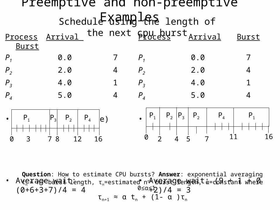
Preemptive and non-preemptive Examples

Question: How to estimate CPU bursts? Answer: exponential averagingtn = nth burst length, τn=estimated nth burst length, α=constant where 0≤α≤1

τn+1 ≈ α tn + (1- α )τn

Schedule using the length of the next cpu burstProcess Arrival

Burst

P1 0.0 7

P2 2.0 4

P3 4.0 1

P4 5.0 4

• SJF (non-preemptive)

• Average wait: (0+6+3+7)/4 = 4

Process Arrival Burst

P1 0.0 7

P2 2.0 4

P3 4.0 1

P4 5.0 4

• SRTF (preemptive)

• Average wait: (9 + 1 + 0 +2)/4 = 3

P1 P3 P2

73 160

P4

8 12

P1 P3P2

42 110

P4

5 7

P2 P1

16

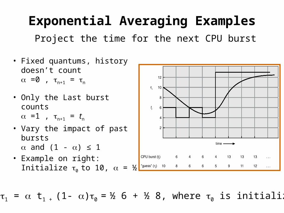
Exponential Averaging Examples

• Fixed quantums, history doesn’t count =0 , n+1 = n

• Only the Last burst counts =1 , n+1 = tn

• Vary the impact of past bursts and (1 - ) ≤ 1

• Example on right: Initialize 0 to 10, = ½

Project the time for the next CPU burst

Example: 1 = t1 + (1- )0 = ½ 6 + ½ 8, where 0 is initialized to 10

Priority Scheduling

• Highest priority wins (Some systems: smallest integer highest priority)

• Priority algorithms can be either preemptive or non-preemptive– SJF is a priority scheduler: priority = predicted next CPU burst– FIFO is a non-preemptive priority scheduler: priority = time waiting

• Preemptive schemes (Round Robin – RR)– Schedule when quantum expires (10-100 millisecond)– Large quantum ≈ FIFO; Small quantum (q) incurs high overhead– Maximum wait is (n-1)*q for processes of the same priority– Each process uses 1/n of CPU (minus scheduling overhead)

• Problem and solution– Problem: Low priority processes may never execute (starvation)– Solution: Increase a process priority as wait time increases (aging)

Assign a priority integer value to each process

Example of RR with Time Quantum = 20

Process Burst Time

P1 53

P2 17

P3 68

P4 24

Compared to SRJ: Worse average turnaround; better response

P1 P2 P3 P4 P1 P3 P4 P1 P3 P3

0 20 37 57 77 97 117 121134 154162

Round Robin Scheduling (RR)

Processes exceeding their time quantum go to the back of the queue

Turnaround Vs. Quantum SizeRound Robin Gantt Chart

Multilevel Queues

MultipleReadyQueues

Multilevel-feedback: Allows processes to migrate between multilevel queues

Design questions and possible answers1.How many queues? A number of interactive foreground priority-based queues; a single background batch queue

2.Which scheduling algorithms? Interactive – RR, Background – FCFS

3.When to upgrade or demote a process? Demote processes whose quantum expires, Promote if I/O to compute ratio falls below threshold

4.Scheduling between queues? Allocate CPU % to each interactive queue. Favor foreground over background

Multilevel Feedback Example

• Three queues – Q0 Processes have 8 millisecond

quantum, FCFS algorithm

– Q1 Processes have 16 millisecond quantum, FCFS algorithm

– Q2 – FCFS

• Scheduling– New jobs enters queue Q0. They

move to Q1 if quantum expires

– Jobs in Q1 receive a new quantum. They move to Q2 if their Q1 quantum expires

Solaris Scheduling

CategoriesInteractive and Time Share

Solaris Dispatch Table

• Priority: a higher number indicates a higher priority. Processes that wait too long get a priority boost.

• Time Quantum: the time quantum for the associated priority

• Time Quantum expired: the priority of a thread that has used its entire time quantum without blocking. It’s priority is demoted.

• Return from sleep: the priority of a thread that is returning from sleeping (such as waiting for I/O). It gets a priority boost.

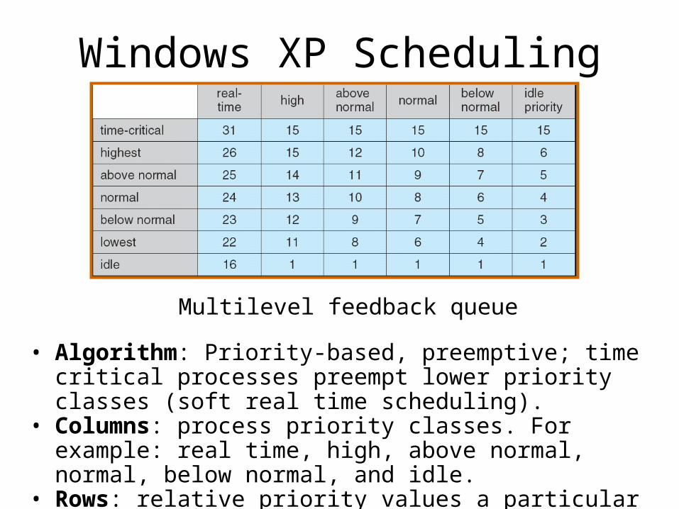
Windows XP Scheduling

Multilevel feedback queue

• Algorithm: Priority-based, preemptive; time critical processes preempt lower priority classes (soft real time scheduling).

• Columns: process priority classes. For example: real time, high, above normal, normal, below normal, and idle.

• Rows: relative priority values a particular process can assume. For example, real time processes can have priorities from 16 to 31.

Linux Scheduling

• Time-sharing algorithm– Higher priority numbers– Schedule process with most

credits– Timer interrupt: reduce credit– Context switch if credits = 0– Re-credit (based on priority

and history ) if no processes have credits left

• Soft Real-time algorithm– Lower priority numbers– Two Posix.1b compliant

classes where highest priority classes always run first• First Class: FCFS• Second Class: Round Robin Quantum length vs. Priority

Linux List of Tasks Indexed According to Priorities

• Constant order O(1) scheduling algorithm with two arrays of run queues

– Active array: ready, not-yet-run tasks

– Expired array: already-ran-and-expired tasks

• Run highest priority active array tasks, move to expired when quanta expires

• If a priority active array empties, swap active/expired arrays. Then re-credit quanta and possibly adjust priority by +/- 5. More process wait time means higher priority

Multiprocessor Scheduling

• Homogeneous processors: same architecture on all processes– Any process can run on any available processor

• Categories of multiprocessing– Asymmetric: One processor controls resources & scheduling– Symmetric: All share resources and scheduling decisions. Each

processor has its own ready queues and data structures.• Load Balancing Algorithms

– Push: Processors push jobs to other processors– Pull: lightly loaded processors pull from other processors– Threshold variable determines when to migrate

• Difficulties in migrating processes– Lots of data to move– Lose cache advantage (must be invalidated and repopulated)– Soft affinity: migration possible; Hard affinity: never migrate

Algorithms are more complex

Thread Scheduling• Local scheduling (PTHREAD_SCOPE_PROCESS)

– The thread library (ex: Pthreads) assigns threads to an available light weight process

– Contention is between active application threads

• Global Scheduling (PTHREAD_SCOPE_SYSTEM)– Kernel schedules threads on available processors– Contention is between kernel threads

• JVM Scheduling – non-preemptible (cooperative) unless– A thread blocks or yields execution– A higher priority thread becomes runnable– Note: Java programs yield() to ensure fair share processing

• while (true) {// perform some task; Thread.yield();}• Yield() gives control to Another thread of equal priority

– Note: some systems support preemption

Pthreads Exampleint main(int argc, char *argv[])

{ int i, scope, THREADS = 10;

pthread_t tid[THREADS];

pthread_attr_t attr;

pthread_attr_int(&attr); // get the default attributes

// Set for kernel level scheduling

pthread_attr_setscope(&attr, PTHREAD_SCOPE_SYSTEM);

for (i=0; i<THREADS; i++) pthread_create(&tid[i], &attr, run, NULL);

for (i=0; i<THREADS; i++) pthread_join(tid[i], NULL);}

void *run(void *param)

{ /* do something */

pthread_exit(0); } The NULL in create is for passing arguments

The Null in join is for a return value

Java Threads• Create thread: implements Runnable or extends thread

• Spawn thread: call the start() method

• Scheduling: dependent on underlying OS.

• Threads run till:– Quantum expires

– Blocks for I/O

– Leave run() method

– Sleep() or yield()

• Priority range (Between 1 and 10)– Thread.MIN_PRIORITY (1)

– Thread.NORM_PRIORITY (5)

– Thread.MAX_PRIORITY (10)

• Set priority: thread.setPriority(Thread.NORM_PRIORITY);

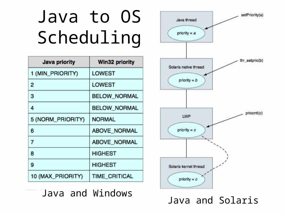
Java to OS Scheduling

Java and WindowsJava and Solaris

Evaluating Scheduling Algorithms• Paper and Pencil Gantt

chart analysis• Run predetermined

work loads• Run simulations using

queuing theory• Actual live

implementations. Humans are good at defeating the best algorithms