a markov decision process model for the optimal dispatch of

A MARKOV DECISION PROCESS MODELFOR THE OPTIMAL DISPATCH OF

MILITARY MEDICAL EVACUATION ASSETS

THESIS

Sean K. Keneally, Major, USA

AFIT-ENS-14-M-15

DEPARTMENT OF THE AIR FORCEAIR UNIVERSITY

AIR FORCE INSTITUTE OF TECHNOLOGY

Wright-Patterson Air Force Base, Ohio

DISTRIBUTION STATEMENT A. APPROVED FOR PUBLIC RELEASE;

DISTRIBUTION UNLIMITED

The views expressed in this thesis are those of the author and do not reflect the officialpolicy or position of the United States Air Force, United States Army, United StatesDepartment of Defense or the United States Government. This is an academic workand should not be used to imply or infer actual mission capability or limitations.

AFIT-ENS-14-M-15

A MARKOV DECISION PROCESS MODEL FOR THE OPTIMAL

DISPATCH OF MILITARY MEDICAL EVACUATION ASSETS

THESIS

Presented to the Faculty

Department of Operational Sciences

Graduate School of Engineering and Management

Air Force Institute of Technology

Air University

Air Education and Training Command

in Partial Fulfillment of the Requirements for the

Degree of Master of Science (Operations Research)

Sean K. Keneally, BS, MS

Major, USA

March 2014

DISTRIBUTION STATEMENT A. APPROVED FOR PUBLIC RELEASE;

DISTRIBUTION UNLIMITED

AFIT-ENS-14-M-15



Sean K. Keneally, BS, MSMajor, USA

Approved:

//signed// 13 March 2014

Maj Matthew J.D. Robbins, Ph.D.(Chairman)

Date

//signed// 13 March 2014

LTC Brian J. Lunday, Ph.D. (Reader) Date

AFIT-ENS-14-M-15

Abstract

We develop a Markov decision process (MDP) model to examine military medical

evacuation (MEDEVAC) dispatch policies in a combat environment. The problem of

deciding which aeromedical asset to dispatch to which service request is complicated

by the threat conditions at the service locations and the priority class of each casu-

alty event. We assume requests for MEDEVAC arrive sequentially, with the location

and the priority of each casualty known upon initiation of the request. The United

States military uses a 9-line MEDEVAC request system to classify casualties using

three priority levels: urgent (A), priority (B), and routine (C). Multiple casualties can

be present at a single casualty event with the highest priority casualty determining

the priority level for the casualty event. An armed escort may be required depend-

ing on the threat level indicated by the 9-line MEDEVAC request. The proposed

MDP model indicates how to optimally dispatch ambulatory helicopters to casualty

events in order to maximize the steady-state system utility. The utility gained from

servicing a specific request depends on the number of casualties, the priority classes

for each of the casualties therein, and the locations of both the servicing ambulatory

helicopter and casualty event. Instances of the dispatching problem are solved using

a value iteration dynamic programming algorithm. Computational examples are used

to investigate optimal dispatch policies under different threat situations and potential

armed escort delay. The computational examples are based upon combat operational

scenarios with United States Army MEDEVAC units in support of Operation En-

during Freedom (OEF) in Afghanistan. Results indicate that a myopic policy is not

always the best method to use for quickly dispatching MEDEVAC units under differ-

iv

ing threat conditions while conducting combat operations under a variety of different

parameters.

Key words: Emergency Medical Dispatch, Markov decision processes, medical

evacuation (MEDEVAC)

v

This research is dedicated to the soldiers that gave their lives in support of Operation

Iraqi Freedom and Operation Enduring Freedom; may this research continue in order

to provide the best medical evacuation system possible, for those who follow in your

footsteps. Special thanks goes to my wife and two children for their unconditional

love and support throughout the process of this research.

vi

Acknowledgements

I would like to thank Maj Matthew J.D. Robbins, Ph.D. for working with me as

my advisor and for his relentless efforts in assisting me with the concepts in and de-

velopment of this manuscript. Great appreciation also goes to LTC Brian J. Lunday,

Ph.D. for putting forth extra effort in being my reader and for his assistance in the

structure and composition of this manuscript. Special thanks goes to Maj Kristy L.

Moore and CPT James A. Jablonski for their invaluable assistance with portions of

the MATLAB code in order to generate the computational results necessary to make

this paper a success. Lastly, I would like to thank the US Army Medical Evacuation

Proponency for its encouragement and feedback on this line of research.

Sean K. Keneally

vii

Table of Contents

Page

Abstract . . . . . . . . . . . . . . . . . . . . . . . . . . . . . . . . . . . . . . . . . . . . . . . . . . . . . . . . . . . . . . . iv

Acknowledgements . . . . . . . . . . . . . . . . . . . . . . . . . . . . . . . . . . . . . . . . . . . . . . . . . . . . . vii

List of Figures . . . . . . . . . . . . . . . . . . . . . . . . . . . . . . . . . . . . . . . . . . . . . . . . . . . . . . . . . . ix

List of Tables . . . . . . . . . . . . . . . . . . . . . . . . . . . . . . . . . . . . . . . . . . . . . . . . . . . . . . . . . . . . x

I. Introduction . . . . . . . . . . . . . . . . . . . . . . . . . . . . . . . . . . . . . . . . . . . . . . . . . . . . . . . . 1

II. Background . . . . . . . . . . . . . . . . . . . . . . . . . . . . . . . . . . . . . . . . . . . . . . . . . . . . . . . . 5

III. Problem Description . . . . . . . . . . . . . . . . . . . . . . . . . . . . . . . . . . . . . . . . . . . . . . . . 14

IV. Model Formulation . . . . . . . . . . . . . . . . . . . . . . . . . . . . . . . . . . . . . . . . . . . . . . . . . 19

V. Computational Example: Four zones and four MEDEVACunits . . . . . . . . . . . . . . . . . . . . . . . . . . . . . . . . . . . . . . . . . . . . . . . . . . . . . . . . . . . . . 25

5.1 Estimating Model Parameters . . . . . . . . . . . . . . . . . . . . . . . . . . . . . . . . . . . . 255.2 Results & Optimal Policies . . . . . . . . . . . . . . . . . . . . . . . . . . . . . . . . . . . . . . 345.3 MEDEVAC System Under Different Scenarios and

Policies . . . . . . . . . . . . . . . . . . . . . . . . . . . . . . . . . . . . . . . . . . . . . . . . . . . . . . . 435.3.1 Performance of Different Policies Applied to

Stability Operations (Base Case) . . . . . . . . . . . . . . . . . . . . . . . . . . . 465.3.2 Stability Operations With Increased Armed

Escort Delay Parameters . . . . . . . . . . . . . . . . . . . . . . . . . . . . . . . . . . 505.3.3 Stability Operations During Heightened Enemy

Activity . . . . . . . . . . . . . . . . . . . . . . . . . . . . . . . . . . . . . . . . . . . . . . . . . 525.4 Sensitivity Analysis . . . . . . . . . . . . . . . . . . . . . . . . . . . . . . . . . . . . . . . . . . . . . 55

5.4.1 Change in Arrival Rate . . . . . . . . . . . . . . . . . . . . . . . . . . . . . . . . . . . . 555.4.2 Change in φi, the proportion of 9-line

MEDEVAC requests in demand Zone i . . . . . . . . . . . . . . . . . . . . . . 59

VI. Conclusions . . . . . . . . . . . . . . . . . . . . . . . . . . . . . . . . . . . . . . . . . . . . . . . . . . . . . . . 63

Appendix: Table of Notation . . . . . . . . . . . . . . . . . . . . . . . . . . . . . . . . . . . . . . . . . . . . . 68Bibliography . . . . . . . . . . . . . . . . . . . . . . . . . . . . . . . . . . . . . . . . . . . . . . . . . . . . . . . . . . . 71Vita . . . . . . . . . . . . . . . . . . . . . . . . . . . . . . . . . . . . . . . . . . . . . . . . . . . . . . . . . . . . . . . . . . . 74

viii

List of Figures

Figure Page

1 MEDEVAC Mission Timeline . . . . . . . . . . . . . . . . . . . . . . . . . . . . . . . . . . . . 16

2 MEDEVAC and MTF locations with Casualty ClusterCenters . . . . . . . . . . . . . . . . . . . . . . . . . . . . . . . . . . . . . . . . . . . . . . . . . . . . . . . . 28

3 Casualty Events throughout southern Afghanistan . . . . . . . . . . . . . . . . . . 28

4 Number of Coalition Forces KIA in 2010 . . . . . . . . . . . . . . . . . . . . . . . . . . . 44

5 Stability Operations (Base Case) RTT = 60 . . . . . . . . . . . . . . . . . . . . . . . . 47

6 Stability Operations (Base Case) RTT = 90 . . . . . . . . . . . . . . . . . . . . . . . . 48

7 Stability Operations With Increased Armed EscortDelay Parameters, RTT = 60. . . . . . . . . . . . . . . . . . . . . . . . . . . . . . . . . . . . . 52

8 Stability Operations With Increased Armed EscortDelay Parameters, RTT = 90. . . . . . . . . . . . . . . . . . . . . . . . . . . . . . . . . . . . . 53

9 Stability Operations With Increased Enemy Activity,RTT = 60 . . . . . . . . . . . . . . . . . . . . . . . . . . . . . . . . . . . . . . . . . . . . . . . . . . . . . 54

10 Stability Operations With Increased Enemy Activity,RTT = 90 . . . . . . . . . . . . . . . . . . . . . . . . . . . . . . . . . . . . . . . . . . . . . . . . . . . . . 55

11 Change in Arrival Rate, λ = 130

, RTT = 60 . . . . . . . . . . . . . . . . . . . . . . . . . 57

12 Change in Proportion of 9-line MEDEVAC requests forZone i, φ1 = 0.35, RTT = 60 . . . . . . . . . . . . . . . . . . . . . . . . . . . . . . . . . . . . . 60

ix

List of Tables

Table Page

1 Expected Response Time (minutes) . . . . . . . . . . . . . . . . . . . . . . . . . . . . . . . 30

2 Expected Service Time (minutes) . . . . . . . . . . . . . . . . . . . . . . . . . . . . . . . . . 30

3 Utility (60 minute RTT) . . . . . . . . . . . . . . . . . . . . . . . . . . . . . . . . . . . . . . . . . 32

4 Utility (90 minute RTT) . . . . . . . . . . . . . . . . . . . . . . . . . . . . . . . . . . . . . . . . . 33

5 Optimal Policy for State (0,0,0,0), RTT = 60 minutes . . . . . . . . . . . . . . . 34

6 Optimal Policy for State (w,0,0,0), RTT = 60 minutes . . . . . . . . . . . . . . . 35

7 Optimal Policy for State (0,x,0,0), RTT = 60 minutes . . . . . . . . . . . . . . . 36

8 Optimal Policy for State (0,0,y,0), RTT = 60 minutes . . . . . . . . . . . . . . . 36

9 Optimal Policy for State (0,0,0,z), RTT = 60 minutes . . . . . . . . . . . . . . . 37

10 Optimal Policy for State (w,x,0,0), RTT = 60 minutes . . . . . . . . . . . . . . . 37

11 Optimal Policy for State (0,0,y,z), RTT = 60 minutes . . . . . . . . . . . . . . . . 38

12 Optimal Policy for State (w,0,0,z), RTT = 60 minutes . . . . . . . . . . . . . . . 39

13 Optimal Policy for State (w,0,y,0), RTT = 60 minutes . . . . . . . . . . . . . . . 39

14 Optimal Policy for State (0,x,0,z), RTT = 60 minutes . . . . . . . . . . . . . . . 40

15 Optimal Policy for State (0,0,0,0), RTT = 90 minutes . . . . . . . . . . . . . . . 41

16 Optimal Policy for State (w,x,0,0), RTT = 90 minutes . . . . . . . . . . . . . . . 41

17 Optimal Policy for State (0,0,y,z), RTT = 90 minutes . . . . . . . . . . . . . . . . 42

18 Optimal Policy for State (0,0,y,0), RTT = 60 minutes,Increased AE delay . . . . . . . . . . . . . . . . . . . . . . . . . . . . . . . . . . . . . . . . . . . . . 51

19 Optimal Policy for State (w,0,0,z), RTT = 60 minutes,Increased AE delay . . . . . . . . . . . . . . . . . . . . . . . . . . . . . . . . . . . . . . . . . . . . . 51

20 Optimal Policy for State (0,0,0,0), RTT = 60 minutes,λ = 1

30. . . . . . . . . . . . . . . . . . . . . . . . . . . . . . . . . . . . . . . . . . . . . . . . . . . . . . . . 57

x

Table Page


1. . . . . . . . . . . . . . . . . . . . . . . . . . . . . . . . . . . . . . . . . . . . . . . . . . . . . . . . . 58


2to 1

8. . . . . . . . . . . . . . . . . . . . . . . . . . . . . . . . . . . . . . . . . . . . . . . . . . . . . 58


9to 1

27or λ ≤ 1

80. . . . . . . . . . . . . . . . . . . . . . . . . . . . . . . . . . . . . . . . . . . 58


28to 1

79. . . . . . . . . . . . . . . . . . . . . . . . . . . . . . . . . . . . . . . . . . . . . . . . . . . . 59

25 Optimal Policy for State (0,0,0,0), RTT = 60 minutes,φ1 = 0.22 . . . . . . . . . . . . . . . . . . . . . . . . . . . . . . . . . . . . . . . . . . . . . . . . . . . . . . 60

26 Optimal Policy for State (w,0,0,0), RTT = 60 minutes,φ1 = 0.03 . . . . . . . . . . . . . . . . . . . . . . . . . . . . . . . . . . . . . . . . . . . . . . . . . . . . . . 61

27 Optimal Policy for State (0,0,0,0), RTT = 60 minutes,φ1 = 0.078 . . . . . . . . . . . . . . . . . . . . . . . . . . . . . . . . . . . . . . . . . . . . . . . . . . . . . 61

28 Optimal Policy for State (0,0,0,0), RTT = 60 minutes,φ1 = 0.12 . . . . . . . . . . . . . . . . . . . . . . . . . . . . . . . . . . . . . . . . . . . . . . . . . . . . . . 62

29 Optimal Policy for State (0,0,y,0), RTT = 60 minutes,φ1 = 0.065 . . . . . . . . . . . . . . . . . . . . . . . . . . . . . . . . . . . . . . . . . . . . . . . . . . . . . 62

xi



I. Introduction

For United States military forces operating in a combat environment, there are

two options for transporting a casualty to the nearest medical facility. The first option

is to conduct a casualty evacuation (CASEVAC), which is simply transporting the

casualty from the point of injury to the nearest appropriate medical facility without

dedicated personnel to provide medical care enroute. The second option is to conduct

a medical evacuation (MEDEVAC), which requires a 9-line MEDEVAC request sub-

mission and includes dedicated medical personnel to treat the casualty during transit.

The MEDEVAC mission commonly refers to the use of dedicated rotary wing aircraft

(i.e., ambulatory helicopters) equipped with medical personnel and equipment [10]. 1

An important task during combat operations, MEDEVAC missions are primarily

conducted by the United States Army. MEDEVAC provides timely and efficient

medical treatment and transportation for casualties on the battlefield enroute to

the nearest required medical facility. Revolutionizing the level of medical treatment

a casualty receives in a timely manner, MEDEVAC missions greatly increase the

probability of a patient’s survivability [9].

The concept of extracting casualties from the battlefield during combat in order

to preserve life was introduced during the American Civil War. The CASEVAC and

MEDEVAC systems continually improved during the next seven major American

conflicts, from the Spanish-American War in 1898 to the War on Terror in 2014. Such

1With the exception of Sections 1 and 2, in this paper we use the term MEDEVAC in referenceto ambulatory helicopters only

1

evolvement consisted of using horse-drawn wagons for CASEVAC in the Spanish-

American War in 1898, motorized ground-vehicles for CASEVAC in World War I,

helicopters for CASEVAC in World War II and the Korean War, to eventually using

helicopters for MEDEVAC beginning during the Vietnam War; This method continues

to be the current primary method of MEDEVAC today. With over a century of

development and technological advancement, the current MEDEVAC system is quite

successful in preserving the lives of many wounded soldiers [21]. However, challenges

remain.

Challenges in the current MEDEVAC system include optimizing the location of

MEDEVAC units, determining dispatch policies, and repositioning units following a

mission. Much research over the past four decades seeks to optimize both the military

and civilian emergency systems [19]. These studies analyze several different aspects

of optimizing the emergency response systems: ambulance location, repositioning

the ambulances post mission, and ambulance dispatch policy considering response

time, patient survivability probability, and patient priority level. While much of

the research since the late 1960’s focuses on the civilian emergency response system,

numerous studies analyze the MEDEVAC system quite extensively as well.

Many authors analyze problems similar to those mentioned above but in a combat

environment. For example, Fulton et al. [16] analyze deployable hospital locations,

MEDEVAC unit location, and the MEDEVAC dispatch policy in order to minimize

response time. Bastian [3] analyzes how to position MEDEVAC units in order to

maximize their coverage capability. Our paper also considers an emergency response

system operating in a combat environment. We examine the problem of optimally

dispatching ambulatory helicopters to prioritized casualty events in order to maximize

steady state system utility. Our dispatch policy is based on the location of idle

MEDEVAC units, the location of the casualty event, the number of casualties within

2

the casualty event, and the priority of the casualties at the casualty event. We

define the individual casualty priority levels from the field medical service technician

student manual [12]. They are as follows: Urgent (A) means the casualty must be

evacuated as soon as possible or within two hours due to possible loss of life, limb, or

eyesight; Priority (B) means the casualty must be evacuated within four hours and

the condition can worsen to Urgent (A); Routine (C) means the casualty must be

evacuated within 24 hours.

We formulate an infinite-horizon, undiscounted, average reward Markov decision

process (MDP) that determines how to optimally dispatch MEDEVAC helicopters to

casualty events on the battlefield in order to maximize the steady-state average of

system utility. A computational example is applied to a MEDEVAC system forward

deployed in Afghanistan in support of combat operations. We analyze the optimal

policies and the effect that an armed escort requirement under specified threat con-

ditions has on the optimal performance of these policies and compare them with a

myopic policy (i.e., simply dispatching the closest unit to each casualty). We assume

that the medical treatment facility (MTF) and combat support hospital (CSH) loca-

tions are fixed, and that all MEDEVAC helicopters have the same capacities and can

be configured to meet the mission requirements specified by the 9-line MEDEVAC

request.

This paper is organized as follows. Section 2 presents further background on

MEDEVAC and provides a review of pertinent literature. Section 3 provides a de-

scription of the problem for which we develop our model. Section 4 describes the

general MDP model we use to determine an optimal MEDEVAC dispatch policy in

the context of the problem. Section 5 describes an application of the specific MDP

model to the analysis of an example based on current day combat operations in

3

Afghanistan. Section 6 provides conclusions and directions for future research.

4

II. Background

Howard [21] points out that before the American Civil War the notion of evacuat-

ing casualties from the battlefield and rendering medical aid to them while en route to

the nearest medical facility was nothing more than an afterthought in the US Army’s

doctrine. With a total of approximately 620,000 soldiers killed in action during the

Civil War, the need for such a service was quickly realized [8]. In 1862, after sev-

eral battles resulted in thousands of wounded soldiers remaining on the battlefield

for days, many of whom took it upon themselves to walk unaided back to friendly

territory, a solution was conceived. Jonathan Letterman, the Medical Director of the

Army of the Potomac, began developing a system for evacuating casualties from the

front lines of the battlefield. His system required that the military dedicate personnel

and resources to the mission of evacuating casualties. This system was standardized

during the Spanish-American War in 1898. Nearly two decades later, World War I

saw numerous advancements in medical technology that resulted in the improvement

of the CASEVAC mission. The first aerial CASEVAC mission occurred during this

war using a modified French airplane. World War II saw many more medical ad-

vancements, but the idea of an aerial MEDEVAC was disregarded by top levels of

the military due to the risk to the casualties. Although this negative outlook halted

nearly all battlefield MEDEVACs, the first large-scale combat aero-medical evacua-

tion occurred in 1942 and was followed by several more until the end of the war in

1945. At the war’s end, more than 1.1 million casualties had been medically evacu-

ated by airplane. Although using air assets to medically evacuate casualties directly

from the battlefield did not occur often at this time, the first rotary wing CASEVAC

mission took place in 1944 near Mawla, Burma where casualties were rescued from

stranded forces [21].

5

As the technology of rotary wing aircraft advanced between World War II and the

Korean War, the Secretary of Defense directed that the primary means of CASEVAC

for sick and injured soldiers during war or peacetime would be by air. Therefore,

helicopters were first used as the primary vehicle for evacuating casualties during

the Korean War, and their use was further perfected during the Vietnam War with

the production of the Bell UH-1 Iroquois, or Huey, helicopter. This aircraft accom-

modated more litters and provided the essential space necessary to conduct in-flight

medical treatment. Today, over half a century later, the helicopter, now the UH-60

Blackhawk, continues to be the primary means of MEDEVAC [21].

Over the past four decades, many studies focus on optimizing emergency response

systems for both civilian and military applications. Past research examines the orig-

inating locations of the emergency units, the dispatch policies that stipulate which

unit responds to which service call, and the repositioning of emergency units to spe-

cific locations to improve system response times. In the last decade, the US Army

has implemented the results of that research during combat operations in Iraq and

Afghanistan.

The MEDEVAC mission is heavily relied upon for current combat operations

in Afghanistan due to the rugged terrain and austere environment. Between 2007

and 2008, over 2060 MEDEVAC missions were flown to evacuate more than 3200

casualties, of which 30% of the casualties were classified as Urgent (A) [20]. The

stated MEDEVAC goal, as directed by the Secretary of Defense, is to transport

an urgent casualty to an appropriate medical facility within 60 minutes [17] from

the receipt of the 9-line MEDEVAC request. In 2007, 12% of MEDEVAC mission

service times were outside the two-hour maximum timeline for an Urgent patient.

North Atlantic Treaty Organization (NATO) forces reduced that figure to 7% by 2008

simply by operationally improving command and control and increasing the number

6

of MEDEVAC aircraft. As a result, despite a higher operational tempo and increased

violence during those years, the rate of soldiers killed in action (KIA) decreased while

the rate of soldiers wounded in action (WIA) increased [20]. This result indicates an

improvement in the MEDEVAC system.

Although recent improvements have been made in the MEDEVAC system, differ-

ent aspects of the system still require investigation. The Army’s MEDEVAC policies

and procedures must continue to adapt to changes in enemy tactics. This fact is

critically important when reviewing and optimizing recent MEDEVAC policies and

procedures because, unlike enemies that adhere to the Geneva Convention, the in-

surgents in Afghanistan consider medical vehicles to be viable targets. Garrett [17]

points out that, despite the clearly identifiable red cross marking, MEDEVAC aircraft

operating in Afghanistan sustain the same ratio of small arms fire hits as other armed

aircraft. As a result, many areas in Afghanistan require the MEDEVAC unit to be

accompanied by an armed escort. This is an essential factor that cannot be ignored.

This requirement has the adverse effect of potentially incurring a significant amount

of response time due to engine warm-up and weapon systems inspections, among other

factors [20]. Although Garrett [17] states that from January 2010 to April 2012, only

31% of MEDEVAC missions required an armed escort, and of those missions only 4%

of them were delayed as a result of the armed escort units, extra time spent wait-

ing for armed escort availability causes an increase in MEDEVAC response time, no

matter how infrequently it is needed.

Another problem with the current MEDEVAC system in Afghanistan involves the

amount of acceptable coverage throughout the country. Hartenstein [20] shows the

MEDEVAC coverage capabilities in Afghanistan and points out that adequate service

to most areas in the country can be delivered within a two-hour response time, where

response time is defined as the time it takes for the unit to transport the individual(s)

7

from the casualty site to the appropriate medical facility from the receipt of a 9-line

MEDEVAC request. However, when that response time requirement decreases to 60

minutes in Afghanistan, numerous gaps exist in coverage capabilities due to the vast

expanse of the region.

Hartenstein [20] argues that a significant improvement in response time would

not be achieved even if the number of MEDEVAC units and the number of medical

facilities is increased. This indicates that system improvements must focus elsewhere,

possibly with an optimal dispatch policy of the MEDEVAC unit considering the

possibility of an armed escort delay. While this study focuses on the conflict in

Afghanistan, it is intended to be useful in future conflicts and training environments

as well.

The decision-making process in the emergency response system is very complex,

whether it is the civilian EMS system or the military MEDEVAC system during

combat operations. Multiple factors are involved in each step of the process such as

district location, the number of servers (i.e., MEDEVAC units) per district, dispatch

policy, server location, repositioning the server location, or whether to focus on re-

sponse time or patient survivability as the objective. Various methods are used to

examine the EMS systems. These methods include, but are not limited to, discrete

optimization, stochastic modeling, queuing, and simulation modeling [26].

Research from the late 1960’s and 1970’s focuses primarily on the civilian EMS

system. These studies examine aspects such as the optimal placement of emergency

vehicles, including both original placement and relocation, to provide the fastest

response time. Math programming and stochastic models are often used to solve such

problems. Few studies focus on optimizing the dispatch policy in order to improve the

performance of the EMS system. Even fewer seek to improve the performance of the

MEDEVAC system. Examining the dispatch policy of emergency response vehicles

8

requires a dynamic and stochastic approach such as agent-based simulation or MDP

modeling. Moreover, many EMS systems’ dispatch policies do not take the priority

level of the casualty event into consideration. This results in the nearest emergency

response team fulfilling the requirement with no regard to the void created in the

system by that unit’s temporary absence. This is known as a myopic policy, and such

policies have been proven to be inadequate by many researchers [26, 1, 25].

Bandara et al. [1] mention several studies in which the EMS system greatly im-

proves the patients’ survival probability if their priority level is taken into consider-

ation when deciding which vehicle to dispatch. Therefore, they build a model that

focuses on the urgency level of an emergency call. In order to properly consider the

optimal policies for decision-making at each discrete time epoch, they use the uni-

formization method to convert the continuous-time MDP that they initially develop

into an equivalent discrete-time MDP. Their study reveals that the optimal policy

is to send the closest unit to the most urgent call and the next idle unit to the less

urgent call, regardless of the call order. While this result may seem intuitive, this

dispatch policy quickly becomes complex. For example, it may be more optimal to

dispatch a vehicle that is farther if the closer vehicle is more likely to receive a higher

priority call. This policy essentially rations the closer vehicle in anticipation of a more

urgent request. For problems with several more service zones and ambulances, the

policy might not be as intuitive although EMS systems stand to benefit greatly from

the employment of an optimal policy versus a myopic policy.

Mayorga et al. [26] also examine the dispatch policy within the EMS system. Their

research improves the performance of the EMS system where performance is defined

as the probability of patient survivability as it is correlated with response times.

Before they examine the dispatch policies, however, they examine the number of

districts and district locations by developing a constructive heuristic. Their research

9

provides more depth than previous studies by analyzing the dispatch policies for

inter-district and intra-district situations. An intra-district situation occurs when

a response vehicle within its own district services the call, whereas an inter-district

situation occurs when all response vehicles within a district area are busy and the call

must be serviced by a response vehicle from a different district. For the inter-district

policy, either a myopic policy (closest vehicle responds) or a heuristic policy (e.g., as

developed in Bandara et al. [1]) is used. While the myopic policy is the most widely

used policy in the EMS system, the heuristic policy considers the priority of the call

as well as the workload of each crew. For such an implementation, a utilization factor

is used in order to consider the workload of each crew. For the intra-district policy,

two policies are considered. The first policy assumes that a sister emergency service

(fire department or police department) would respond. The military equivalent of this

during combat operations would be to have the casualty’s unit conduct first aid and

transport him/her to the nearest CSH or MTF using its own vehicles, a quick reaction

force (QRF), or non-medical helicopter; this is known as a non-standard CASEVAC.

The second policy uses the heuristic policy that Bandara et al. [1] developed and

allows a response vehicle from another district to cross boundary lines.

While examining the dispatch policy within the EMS system, McLay & Mayorga

[28] also analyze the optimization problem with regard to classification errors. They

focus on the patients’ urgency level with an overall objective of maximizing the aver-

age long run utility of the EMS system, rewarding the expected coverage of high-risk

patients. The response time threshold (RTT) that they utilize within their utility

calculations, however, is much lower than the RTT used in our calculations because

they define the response time as the time it takes from when the ambulance is dis-

patched to when it arrives at the injury site. The utilities used in their model are

dependent on both the patient and the hospital locations. Similar to the research

10

done by Bandara et al. [1], they use the uniformization method in order to convert

their initially developed continuous-time MDP into an equivalent discrete-time MDP.

Our paper follows much of the work of Bandara et al. [1] and McLay & Mayorga

[28], given that we also focus much effort on the priority level of the call. We also ini-

tially develop a continuous-time MDP and use the uniformization method to convert

it to a discrete-time MDP in order to allow the stipulation of an optimal dispatch

policy wherein decisions are made at discrete-time events. We design our model so

that the actions are dependent on the locations of the MEDEVAC units, casualty

event, and casualty event classification. We define our objective as maximizing the

average long-run system utility, as does McLay & Mayorga [28]. Our research is also

similar to Mayorga et al. [26] in that our approach allows an inter-district policy. All

four papers, including this one, adopt a stochastic approach in the development of a

MDP. However, this paper focuses on a military application and therefore has several

complex aspects that are not examined in previous research.

Fulton et al. [16] and Bastian [2] examine stochastic optimization for the alloca-

tion of MEDEVAC units in steady-state combat operations. Fulton et al. [16] present

a stochastic optimization model that relocates deployable hospitals, reallocates hos-

pital beds, and determines where emergency response vehicles (both air and ground

MEDEVAC) should be located prior to a 9-line MEDEVAC request. Their objective

is to minimize the amount of time it takes for the MEDEVAC unit to respond and

transport the casualty or casualties to the appropriate medical facility. Fulton et al.

[16] describe a model that focuses on patient severity in order to make the dispatch

decision rather than the proximity to the patient. Their patient severity is deter-

mined from the historical data collection of patients’ injury severity scores (ISS) from

Operation Iraqi Freedom (OIF). They make many of the same assumptions we make

in this paper: since the missions are being conducted during stability operations, the

11

number of helicopters, ground ambulances, and crew members are fixed. Their idea

of using ISS patient survival probabilities in the model is loosely based on the re-

search by Silva & Serra [31] regarding the importance of recognizing priority levels of

patients. The work by Bastian [2] describes a multi-criteria modeling approach that

optimizes the emplacement of MEDEVAC assets. Specifically, his work maximizes

casualty demand coverage and minimizes MEDEVAC spare capacity and site attack

vulnerability, whereas our research provides an optimal dispatch policy in order to

maximize the average long-run system utility.

The work by Schmid [30] uses approximate dynamic programming (ADP) in order

to determine optimal policies that minimize response times. Using real data from the

EMS system in Vienna, Austria, Schmid [30] suggests that a dispatch policy that

deviates from the ordinary dispatch policies used can result in a nearly 13% decrease

in expected system response time. Service calls used in the model from this data were

generated using a spatial Poisson process, which is the same type of process that we

use and describe at the end of Section 3. Although their paper examines ambulance

relocation and considers a civilian EMS system and we do not, more similarities than

differences exist between our research. For example, the graphical representation

that Schmid [30] offers in his Problem Description section is used as a basis for our

MEDEVAC Mission Timeline, as shown later in Figure 1.

Many more research studies relate at least topically to our problem and provide

important insight into what has already been studied. For example, Berman [4] fo-

cuses on repositioning ambulances for follow-on service calls to minimize expected

long-term travel times within the system. In his research, the dispatcher uses a my-

opic policy and only considers repositioning idle ambulances in order to compensate

for areas not covered by busy ambulances. Maxwell et al. [25] use ADP to make deci-

sions on where to redeploy ambulances within the EMS system in order to maximize

12

the number of calls reached within a delay threshold. Erkut et al. [13] incorporate a

survival function into existing covering models in order to generate new ambulance

location models. More useful in our research, while considering our motivating prob-

lem in Afghanistan, Chanta et al. [5] focus on ambulance coverage for rural areas.

Since many missions in Afghanistan are conducted in an austere, rural environment,

the trade-off between efficiency (coverage) and equity between rural and urban zones

examined in their research provides some relevance. However, their particular re-

search focuses on developing a covering location model specific to ground ambulatory

care. All of these papers provide possible methodologies on how to examine problems

concerning the emergency response system and offer contributions to the development

of our research.

13

III. Problem Description

In the remainder of this paper we use the term MEDEVAC to refer to ambulatory

helicopters only. MEDEVAC requests are submitted with very little, if any, lead

time. This means that there is no time to prepare for them, and a quick response

is necessary in order to achieve success in such a mission. To complicate matters,

many situations with a high threat level may require a team of armed helicopters

to escort the MEDEVAC unit to the casualty site, creating the potential for further

delays in the response time. Consequently, the MEDEVAC system must be extremely

flexible and eliminate any decision-making delays in order to optimize its performance.

Developing an optimal policy for such decision-making assists in making this possible.

The assumptions for the model we develop for this problem are below:

We consider three types of calls: Urgent (Category A), Priority (Category B),

Routine (Category C). 9-line MEDEVAC requests use the same three priorities in

order to classify casualties. All emergency types (A, B, or C) can be serviced by

any MEDEVAC platform; therefore, we assume all necessary additional equipment

is located on every MEDEVAC helicopter. The classification of the casualty event is

defined as the highest classification level present at the casualty event (i.e., the most

severe casualty).

A single casualty event can have between one and four casualties. Athough more

than four casualties can occur on a battlefield, placing this constraint on our model

allows only one MEDEVAC aircraft/unit to be dispatched for each casualty event.

This

Response and service times are independent of the casualty event classification.

Although a Routine casualty event allows a response time of 24 hours in combat

situations, we assume that all 9-line MEDEVAC requests are serviced immediately,

14

regardless of the priority classification, if a MEDEVAC unit is available. This enables

us to better examine the dispatch process properly.

There is zero-length queue for casualties; if a 9-line MEDEVAC request cannot

be serviced immediately, we assume a non-standard CASEVAC (e.g., non-medical

ground or air platform) is conducted. These are common missions according to Black-

hawk pilots and OEF veterans [15].

Inter-zone policies, where a MEDEVAC unit from an adjacent casualty zone can

be dispatched to service the 9-line request, are always allowed. This allows nearby

MEDEVAC units to assist with 9-line MEDEVAC requests if needed. It also creates

the need for the model to decide which MEDEVAC unit to dispatch to which casualty

event, thereby making the problem interesting.

Casualties are evacuated to the nearest MTF, thereby assuming that all MTFs in

the area have the same capabilities. Also, if a casualty occurs within close proximity

(e.g., less than a 10 minute drive) of a MTF, the unit on the ground conducts a

CASEVAC in lieu of requesting a 9-line. This is often the case in combat since

transporting a casualty that is near a MTF will take less time than it will to dispatch

a MEDEVAC unit.

After a MEDEVAC unit has completed its mission, it must return to its staging

area before being dispatched again in order to refuel and restock medical supplies.

The MEDEVAC dispatching process for a situation requiring an armed escort

closely follows the process outlined by Schmid [30] and is described in the timeline

depicted graphically in Figure 1.

Once the 9-line MEDEVAC request is received by an approving authority and the

priority level of the request is determined, the appropriate idle MEDEVAC unit is

notified and dispatched to the casualty site.

15

Figure 1. MEDEVAC Mission Timeline

As depicted in Figure 1, the time that the 9-line MEDEVAC request is received

is denoted by t9, the time at which the MEDEVAC unit is assigned to the mission is

denoted by M9, and the time at which the MEDEVAC unit departs is denoted by Md.

The amount of time required between the receipt of the 9-line MEDEVAC request,

t9, and the MEDEVAC departure, Md, is the total dispatching time, D. This time

encompasses the process of determining which MEDEVAC unit to dispatch, whether

an armed escort is required or not, which armed escort unit to dispatch, if required,

notifying the units, and finally the mission, helicopter, and personnel preparation

time. MEDEVAC units arrive at the casualty site after traveling for T c minutes and

begin treating and loading the casualty at time wc9 after waiting E minutes for the

armed escort, if required, to arrive. Initial treatment and loading ends when the

MEDEVAC helicopter departs the casualty site enroute to the appropriate medical

facility and is denoted by ec9. The amount of time spent at the casualty site is Lc.

After traveling to the appropriate medical facility for Tm minutes, the casualty is

unloaded from time wm9 to time em9 after which the casualty is inside the medical

16

facility. The total unload time is denoted by Um. Once the casualty is unloaded

at the medical facility, the MEDEVAC unit travels for T s minutes to its respective

staging area. Once the MEDEVAC unit arrives at its staging area after ws9 minutes,

its mission is complete and it becomes available for dispatch once again.

Note that travel times from the staging area to the casualty site, T c, from the

casualty site to an appropriate medical facility, Tm, and from the medical facility

back to the staging area, T s are expected to vary based on the conditions of the

battlefield (e.g., weather conditions, enemy positions, equipment load). The load and

unload times, Lc and Um, respectively, of the casualties also vary.

EMS systems typically refer to response time as the amount of time required to

reach the patient after receiving an emergency call. According to McLay & Mayorga

[27], the rapid response to cardiac arrest situations are a primary focus in the EMS

system. This is because the EMS system is often evaluated on how it responds to

emergency cardiac arrest calls since there is effective treatment for them and they

are highly time sensitive. Also, if the EMS system can respond quickly enough to

a cardiac arrest call, they are more likely to be successful with similar life-or-death

situations. Therefore, it is quite intuitive that the response time for a civilian EMS

system is typically defined as the time between the receipt of the emergency call and

the time the first emergency response vehicle arrives at the injury site [1].

However, the performance of the MEDEVAC system cannot be evaluated by the

same measures as the EMS system since several additional factors are involved when

medically evacuating a casualty from a battlefield. Not only can the load times,

travel times and unload times be much greater and vary by much more, but the

primary cause of death on the battlefield is blood loss, not cardiac arrest. Very

recent improvements have been made in this area by equipping MEDEVAC units

with in-flight blood transfusion capabilities, but not enough data has been generated

17

to alter the MEDEVAC system’s evaluation measure at the time of our research [24].

Garrett [17] reports that 85% of soldiers killed in action (KIA) were a direct result

of blood loss. Thus, we consider it to be far more critical to get the casualty to the

nearest MTF and into surgery than to simply reach him quickly. We define response

time, denoted as Rij, for MEDEVAC j responding to a casualty event in zone i, as

the sum of the dispatch time, D, travel time to the casualty site, T c, potential armed

escort delay, E, the load time at the casualty site, Lc, travel time to the appropriate

MTF, Tm, and the unload time at the MTF, Um:

Rij = D + T c + E + Lc + Tm + Um. (3.1)

Service time, denoted by Vij, is simply the sum of the response time, Rij, and the

travel time back to the staging area, T s:

Vij = Rij + T s. (3.2)

In order to provide a solution to the problem described in this section, we outline

a general model in section 4 that will prove helpful when applied.

18

IV. Model Formulation

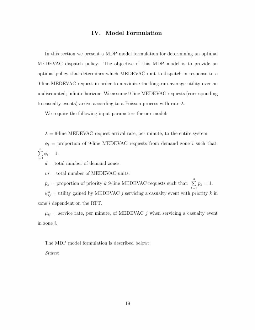
In this section we present a MDP model formulation for determining an optimal

MEDEVAC dispatch policy. The objective of this MDP model is to provide an

optimal policy that determines which MEDEVAC unit to dispatch in response to a

9-line MEDEVAC request in order to maximize the long-run average utility over an

undiscounted, infinite horizon. We assume 9-line MEDEVAC requests (corresponding

to casualty events) arrive according to a Poisson process with rate λ.

We require the following input parameters for our model:

λ = 9-line MEDEVAC request arrival rate, per minute, to the entire system.

φi = proportion of 9-line MEDEVAC requests from demand zone i such that:n∑i=1

φi = 1.

d = total number of demand zones.

m = total number of MEDEVAC units.

pk = proportion of priority k 9-line MEDEVAC requests such that:3∑

k=1

pk = 1.

ψkij = utility gained by MEDEVAC j servicing a casualty event with priority k in

zone i dependent on the RTT.

µij = service rate, per minute, of MEDEVAC j when servicing a casualty event

in zone i.

The MDP model formulation is described below:

States :

19

Let st denote the state of the MEDEVAC system at time t. The state st is the

vector st = (s1t, s2t, ..., smt), where sjt denotes the state of MEDEVAC j at time t:

sjt =

i if MEDEVAC j is responding to a 9-line MEDEVAC request in zone i at time t.

0 if MEDEVAC j is idle at time t.

The state space is defined by S as:

S = {s : s ∈ {0, 1, ..., d}m},with |S| = (d+ 1)m.

For example, consider a system with four MEDEVAC units located in four separate

zones. When MEDEVAC 2 is busy and all other MEDEVAC units are idle we would

have:

st = (0, i, 0, 0),where i ∈ {1, 2, 3, 4}.

Decisions :

The decision in our model is which MEDEVAC unit to dispatch upon receipt of

a 9-line MEDEVAC request in response to a given casualty event. Let A = A(st)

denote the set of available actions in state st upon receipt of a 9-line MEDEVAC

request. Note that in our computational example in Section 5, both intra and inter-

zone responses are allowed; however, MEDEVAC units are restricted from responding

to casualty events more than one zone away from their staging location. That is, in

the event that zone 2 has a casualty event, only MEDEVAC units from zones 1, 2,

or 3 are allowed to respond. Such constraints on the control space can be enforced

as required by the context of the particular problem instance. We assume that if an

idle MEDEVAC unit is located in or adjacent to the zone where the casualty event

occurred, it will be dispatched, not to exceed m actions in each state. For example,

consider the system described above with four MEDEVAC units and four zones; if the

MEDEVAC unit in Zone 3 is busy when a 9-line request is submitted for a casualty

20

event in Zone 3, only MEDEVAC units in Zones 2 or 4 can respond, resulting in

A(st) = {2, 4} when st = (0, 0, y, 0), y 6= 0. In our model, the decisions within the

decision space, A(st), are restricted so that the location of the busy MEDEVAC unit

is independent of the decisions available.

Rewards :

An immediate expected utility ψkij is obtained when MEDEVAC unit j responds

to a casualty event of priority class k that occurs in Zone i. The utility gained

depends on the location and priority of the casualty event as well as the originating

location of the servicing MEDEVAC. While it is often true when studying civilian

EMS systems that rewards can be derived from historical data, in a military context

data is often missing, restricted, or simply irrelevant given new conditions in the

area of operations (e.g., friendly forces are engaging the enemy in different locations).

To obtain the utilities so that we may examine the dynamics of the MEDEVAC

dispatching problem, we simulate the MEDEVAC process.

A single casualty event results in α casualties, where α is a discrete random

variable with support {1,2,...,Nα}. We assume Nα is less than or equal to the servic-

ing capacity of one MEDEVAC helicopter. Each casualty is labeled as Urgent (A),

Priority (B), or Routine (C), corresponding to a priority index level of h = 1,2,3,

respectively. Let q = (q1, q2, q3) denote the probabilities of a casualty belonging to

a particular priority class, where qh is the probability a casualty belongs to priority

class h. Let c = (c1, c2, c3) denote the casualties present at a single casualty event,

where ch is the number of casualties belonging to priority class h. It follows that c is

a multinomial random variable with a probability mass function f(c|α,q) and that

the proportion of priority k 9-line MEDEVAC requests, pk are:

21

pk =

Pr{c1 > 0}, k = 1,

Pr{c1 = 0, c2 > 0}, k = 2,

Pr{c1 = 0, c2 = 0}, k = 3.

The utility rh is gained by servicing a priority h casualty, where r1 > r2 > r3 ≥ 0.

Since we are most interested in servicing casualty events with life-threatening (i.e.,

Urgent) injuries, we adopt a reward structure that incentivizes the servicing of such

casualties and diminishes the importance of servicing a casualty event with no life-

threatening injuries (i.e., Routine). The system gains an expected utility of u(c) for

servicing a single casualty event c, where

u(c) =3∑

h=1

rhchf(ch|α,q).

Since we are able to classify a casualty event according to the most severe injury

sustained at the casualty event prior to the determination of which MEDEVAC to

send, we are able to denote an expected utility

uk(c) =3∑

h=k

rhchf(ch|α,q),

where k is the priority class of the casualty event. Note that k = 1 indicates that

c1 > 0, k = 2 indicates c1 = 0, c2 > 0, and k = 3 indicates c1 = 0, c2 = 0.

There is a requirement that Rij, the response time of MEDEVAC j servicing a

casualty event in Zone i, must not exceed the RTT in order for the system to be

rewarded. This requirement is captured when expressing the expected utility gained

by MEDEVAC j servicing a single priority k casualty event c in Zone i as:

ψkij(c) = uk(c)IRij≤RTT ,

22

where IRij≤RTT is an indicator variable which equals 1 when Rij ≤ RTT and 0

otherwise. When considering a particular instance of our MEDEVAC dispatching

problem, we obtain an average utility ψkij and an expected service rate µij for each

zone, MEDEVAC, and priority permutation by simulating the MEDEVAC process for

a large number of casualty events and computing the mean utilities and service times.

Of particular importance in our simulation procedure is the impact of casualty event

cluster locations on the response times and hence the utilities. Further discussion of

the simulation process is provided in Section 5.

Transitions :

State transitions are Markovian with two possible event types governing the tran-

sition. The first event type is the completion of service by one of the busy MEDEVAC

units. The second event type is the arrival of a 9-line MEDEVAC request which must

be responded to by a MEDEVAC unit if possible.

Optimality Equations :

Puterman [29] argues that the application of uniformization is desirable when

analyzing continuous-time MDPs. Uniformization allows us to state an equivalent

discrete-time MDP problem formulation. We proceed by determining the maximum

rate of transition:

ν = λ+m∑j=1

βj,

where

βj = maxi=1,2,...,d

µij.

We use value iteration to find an optimal policy. Let Jt(st) denote the value of

being in state st during iteration t. We initialize our value function so that J0(s) = 0

23

for all s ∈ S. We follow the basic form of McLay & Mayorga [28] in defining our

optimality equations. They are as follows:

Jn+1(st) =1

ν

[m∑j=1

I{st=i|i>0}µijJn(s1, s2, ..., sj−1, 0, sj+1, ..., sm) (4.1)

+d∑i=1

3∑k=1

λipk maxj∈A(st)

{I{sj=0}Jn(s1, s2, ..., sj−1, i, sj+1, ..., sm) + (ν)(ψkij)}

+ (ν − λ−m∑j=1

I{sj=i|i>0}µij)Jn(st)

], for n = 0, 1, ...,

where

I{sj=i|i>0} = indicator variable that denotes MEDEVAC j is busy in Zone i,

I{sj=0} = indicator variable that denotes MEDEVAC j is idle,

A(st) = the set of available decisions in state st.

The first term in Equation 4.1 describes busy MEDEVAC units becoming idle, the

second term describes new 9-line MEDEVAC requests arriving to the system, where

A(st) represents the available decisions in state st, and the third term describes the

system remaining in the same state with no new 9-line MEDEVAC requests or any

MEDEVAC units becoming idle.

24

V. Computational Example: Four zones and four

MEDEVAC units

In this section, we apply the MDP model to an example set in Afghanistan during

steady state combat operations.

5.1 Estimating Model Parameters

We present an example in which MEDEVAC units are dispatched during steady

state combat operations in support of OEF. The southern portion of Afghanistan is

the area of operation (AO) and is divided into four separate zones, d = 4: Nimroz

province (Zone 1), Helmand province (Zone 2), Kandahar province (Zone 3), and

Zabul province (Zone 4). We use four MEDEVAC helicopters, m = 4, with one

located in each of the four separate zones. The MEDEVAC units transport casualties

to one of two MTFs, located in either Zone 2 or 3. Zones 1 and 4 do not have

MTFs. The placement of medical assets represents a general realism based on past

enemy activity in southern Afghanistan and the author’s combat experience. Based

on historical data, as well as the author’s experience in Afghanistan, the casualty rate

in Zones 2 and 3 are much higher than in Zones 1 and 4.

According to icasualties.org [22], Helmand and Kandahar have been the two most

casualty producing provinces in Afghanistan during OEF with 944 and 544 personnel

killed in action (KIA) alone, respectively. These numbers are compared to six KIAs

in Nimroz and 118 KIAs in Zabul. Although these numbers do not account for the

numerous other casualties that would include personnel wounded in action (WIA),

they provide an approximation of the threat present in each zone. We use this infor-

mation to parameterize φi, the proportion of casualties from Zone i. Straight forward

25

calculations give us casualty proportions per zone of 0.4% in Zone 1, 58.5% in Zone 2,

33.8% in Zone 3, and 7.3% in Zone 4. This gives us φ = (0.004, 0.585, 0.338, 0.073).

These casualty proportions are consistent with the greater number of people,

Afghan citizens as well as enemy and friendly combatants, that are present in both

Helmand and Kandahar. According to the Afghan government, Zones 1-4 have pop-

ulations of approximately 156,000 people, 880,000 people, 1.15 million people, and

289,000 people, respectively [7]. Moreover, according to Department of the Army

[11] as well as the author’s experience in Afghanistan, it is reasonable to expect that

one brigade combat team (BCT) would be assigned Zones 1 and 2 as its area of re-

sponsibility (AOR) and that the BCT would most likely assign the majority of its

combat power to Zone 2 while assigning one task force (TF), which is a reinforced

battalion, to Zone 1. Likewise, one BCT would be assigned Zones 3 and 4 as its AOR

while assigning the majority of its combat power in Zone 3 and one TF to one 4.

The ratio of citizens and combatants in each zone suggests that more casualty events

are expected to occur in Zones 2 and 3. Therefore, the MEDEVAC units located in

Helmand and Kandahar provinces, Zones 2 and 3, respectively, are co-located with

the MTFs.

Actual data for casualty, MEDEVAC unit, and MTF locations are restricted. Mil-

itary medical planners anticipate future operations when estimating casualty event

arrivals. Therefore, in order to compute utilities, we first generate the response and

service times described in Section 3. To avoid using specific data from Afghanistan in

order to maintain operational security while OEF stability operations are on going,

we develop a procedure that leverages military medical planning techniques and the

combat infantry background of the author to model where future casualties may be

sustained. Data from past experiences obviously informs this process, but future op-

erations are important as well; data will certainly change with each unique conflict.

26

Therefore, in the absence of data, we develop a Monte Carlo simulation that uses

casualty cluster centers as a point of reference. Casualty cluster centers are selected

based on their close proximity to main supply routes (MSR) and rivers where popula-

tion groupings are present, since these demographic and geographical features indicate

common sites of attack during missions supporting OEF. Using these casualty clus-

ter centers, we employ a Poisson cluster process to model the arrival and location

of casualty events. Since insurgent attacks against coalition forces in Afghanistan

closely resemble crime patterns, they can be analyzed as a contagion-like process.

The Hawkes spatial generation process (see Kroese & Botev [23] for a discussion)

provides the basis of our collection of utilities as well as response and service time

information. This process models situations where, for a single casualty event, a

number of subsequent events are expected to occur within a close spatial proximity

of the first event according to a Poisson distribution.

We use MATLAB in order to display a map of our AO as shown in Figure 2, and to

determine casualty cluster centers, as well as corresponding casualty events as shown

in Figure 3. We also employ our Monte Carlo simulation and subsequently calculate

the response and service times as well as the utilities for given dispatch decisions.

We used a Toshiba Satellite A505 computer with an Intel Core processor and 4 GB

RAM. The computational time for each MEDEVAC unit was 413.49 seconds.

Figure 2 shows a depiction of the four zones in southern Afghanistan that we use

to generate our data. It also depicts the MEDEVAC locations, one in each zone.

MEDEVACs 1 and 4 are represented by blue diamonds. Recall that Zones 1 and 4 do

not have MTFs. MEDEVACs 2 and 3, co-located with MTFs 2 and 3, respectively,

are represented by blue dots. The casualty cluster centers in each zone are represented

by black dots.

27

Figure 2. MEDEVAC and MTF locations with Casualty Cluster Centers

Figure 3 illustrates several casualty events throughout southern Afghanistan within

a given time period. For simulation purposes, we increase the arrival rate of casualty

events and generate a large number of data points in order to calculate expected

response and service times. This allows us to compute the system utility obtained

when MEDEVAC j responds to a priority k casualty event from Zone i.

Figure 3. Casualty Events throughout southern Afghanistan

28

The data generated for the variables in Equation 3.1 vary with each mission and

therefore are represented as random variables. The details of each variable used to

calculate the response time, Rij, are described in the following five paragraphs.

According to subject matter experts and Blackhawk/MEDEVAC pilots, the flight

speed, which accounts for the travel times, T c and Tm, are each uniformly distributed

over an interval of 120 and 150 knots with a resulting mean of 135 knots [15], [14].

Bastian [2] uses a slightly larger range with a flight speed that is also uniformly

distributed between 120 and 193 nautical-miles per hour, but we choose to use the

tighter flight speed parameters provided by the pilots.

The dispatch time, D, is exponentially distributed. Bastian [2] uses a mean of 20

minutes based on a 2008 MEDEVAC after action review and a standard deviation

of five minutes based on his personal experience. Garrett [17] suggests that only

4% of MEDEVAC missions exceed the 15-minute launch criteria established by the

Commander of the United States Central Command (USCENTCOM). We use a mean

of 15 minutes rather than 20 minutes.

The delay caused by an armed escort, E, is exponentially distributed with a mean

of 10 minutes. According to Garrett [17] there is a 31% chance of a MEDEVAC

mission requiring an armed escort, which we denote as θ1, and of those escorted

missions, approximately 4% are delayed due to issues with the escort aircraft, denoted

by θ2. These parameters are factored into the computation for the expected response

times and therefore the utilities.

The casualty load time, Lc, is exponentially distributed with a mean of 10 minutes.

Bastian [2] uses a triangular distribution with a mean of 10 minutes, a minimum of

five minutes, and a maximum of 15 minutes. While we agree with the 10 minute

mean time, this author’s personal experience in Iraq and Afghanistan suggests that

there is too high of a likelihood for extreme variance when dealing with issues on the

29

ground at the casualty site. Therefore, we believe that an exponential distribution is

more appropriate.

The casualty unload time, Um, is exponentially distributed with a mean of five

minutes as it typically takes much less time to unload the casualty at the MTF than

it does to load the casualty at the initial injury site. Bastian [2] uses a normal dis-

tribution with a mean of five minutes. Again, we agree with the five-minute mean

time but believe that there is a potential for great variance in this case. The mean

response times we calculate are provided in Table 1.

Table 1. Expected Response Time (minutes)

Zone MEDEVAC 1 MEDEVAC 2 MEDEVAC 3 MEDEVAC 4Zone 1 (Nimroz) 47.25 51.29 N/A N/AZone 2 (Helmand) 43.35 39.27 44.69 N/AZone 3 (Kandahar) N/A 46.15 39.49 48.90Zone 4 (Zabul) N/A N/A 59.34 49.90

Once the mean response times are calculated, we compute the mean service times

in accordance to Equation 3.2. The distribution for the flight speed mentioned above

is used for this travel time as well. The mean service times we calculate are provided

in Table 2.

Table 2. Expected Service Time (minutes)

Zone MEDEVAC 1 MEDEVAC 2 MEDEVAC 3 MEDEVAC 4Zone 1 (Nimroz) 53.02 51.29 N/A N/AZone 2 (Helmand) 49.12 39.27 55.23 N/AZone 3 (Kandahar) N/A 56.69 39.49 63.74Zone 4 (Zabul) N/A N/A 59.34 64.74

In this particular computational example, recall that MEDEVAC units are allowed

both intra and inter-zone responses but are restricted from responding to casualties

more than one zone away from their staging location. For example, if there is a

30

casualty in Zone 2, it can be serviced by the MEDEVAC units located in Zones 1, 2

or 3. The casualty is then evacuated to the nearest MTF, MTF 2 in this case. Since

our model in this example applies to a MEDEVAC system with four zones and four

MEDEVAC units, we have the following state space, S = (w, x, y, z):

S = {(0, 0, 0, 0), (w, 0, 0, 0), (0, x, 0, 0), (0, 0, y, 0), (0, 0, 0, z), (w, x, 0, 0), (w, 0, y, 0), (w, 0, 0, z),

(0, x, y, 0), (0, x, 0, z), (0, 0, y, z), (w, x, y, 0), (w, x, 0, z), (0, x, y, z), (w, 0, y, z), (w, x, y, z)},

where

w = 1, 2

x = 1, 2, 3

y = 2, 3, 4

z = 3, 4.

Next, we compute the expected utilities of each MEDEVAC mission for casualty

event classifications of Urgent (A, k = 1), Priority (B, k = 2), and Routine (C,

k = 3). The rewards associated with our model for the MEDEVAC system are

defined by the utility assigned to the selected decision. Recall that the utility rh is

gained by servicing a priority h casualty where r1 > r2 > r3. We let r = (10, 1, 0)

represent the utility gained by servicing a priority h casualty dependent upon the

response time and RTT. We use a RTT of 60 minutes, the US standard directed by

the Secretary of Defense, and 90 minutes, the NATO standard according to Cordell

et al. [6], when computing the utilities of each MEDEVAC mission. Recall that if the

MEDEVAC unit’s response time is within the RTT, the mission gains a utility based

on the number and classification of the casualties evacuated from the casualty event

site. If the response time is greater than the RTT the mission gains a utility of zero.

31

Recall that the sum of the utilities for each casualty within the casualty event

yields the total utility for servicing the 9-line MEDEVAC request. Fulton et al. [16]

report that the probability of a casualty being classified as Urgent (A), Priority (B),

or Routine (C) is 11%, 12%, and 77%, respectively, resulting in q=(0.11,0.12,0.77).

Therefore, since r = (10, 1, 0), each MEDEVAC mission that results in a response time

less than the RTT will gain utilities of 10, 1 and 0 for each Urgent (A), Priority (B),

and Routine (C) casualty, respectively, according to c. For example, if a MEDEVAC

mission returns from responding to a casualty event within the RTT with a casualty

load of one Urgent (A), two Priority (B), and one Routine (C), the system earns a

utility of 12. Note that a casualty classified as Routine (C), h = 3, is not awarded a

utility because it is not life-threatening and we are only concerned with the amount

of lives saved as a function of response time. Tables 3 and 4 summarize the computed

utilities, ψkij, of these computations with both a 60 minute RTT and a 90 minute

RTT, respectively.

Table 3. Utility (60 minute RTT)

Zone Category MEDEVAC 1 MEDEVAC 2 MEDEVAC 3 MEDEVAC 4

Zone 1 (Nimroz)A 8.25 7.67 N/A N/AB 0.85 0.76 N/A N/AC 0 0 N/A N/A

Zone 2 (Helmand)A 8.75 9.12 8.61 N/AB 0.87 0.90 0.86 N/AC 0 0 0 N/A

Zone 3 (Kandahar)A N/A 8.43 9.11 8.11B N/A 0.84 0.91 0.81C N/A 0 0 0

Zone 4 (Zabul)A N/A N/A 6.09 7.92B N/A N/A 0.61 0.79C N/A N/A 0 0

In order to use the utilities to find optimal policies for each state, we determine

the 9-line MEDEVAC request arrival rate to the entire system. Fulton et al. [16]

report that during OIF, an expected 173 casualties moved by air in a given month.

Although we are using OEF as our computational example, we use the data provided

32

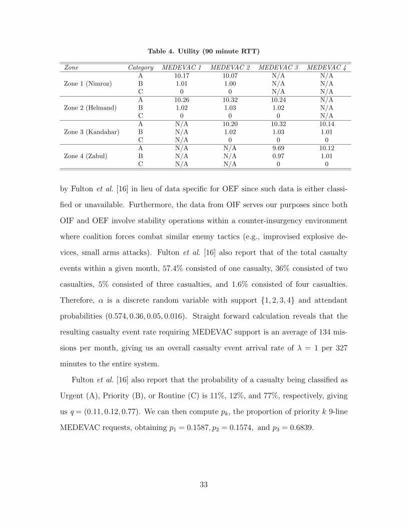
Table 4. Utility (90 minute RTT)

Zone Category MEDEVAC 1 MEDEVAC 2 MEDEVAC 3 MEDEVAC 4

Zone 1 (Nimroz)A 10.17 10.07 N/A N/AB 1.01 1.00 N/A N/AC 0 0 N/A N/A

Zone 2 (Helmand)A 10.26 10.32 10.24 N/AB 1.02 1.03 1.02 N/AC 0 0 0 N/A

Zone 3 (Kandahar)A N/A 10.20 10.32 10.14B N/A 1.02 1.03 1.01C N/A 0 0 0

Zone 4 (Zabul)A N/A N/A 9.69 10.12B N/A N/A 0.97 1.01C N/A N/A 0 0

by Fulton et al. [16] in lieu of data specific for OEF since such data is either classi-

fied or unavailable. Furthermore, the data from OIF serves our purposes since both

OIF and OEF involve stability operations within a counter-insurgency environment

where coalition forces combat similar enemy tactics (e.g., improvised explosive de-

vices, small arms attacks). Fulton et al. [16] also report that of the total casualty

events within a given month, 57.4% consisted of one casualty, 36% consisted of two

casualties, 5% consisted of three casualties, and 1.6% consisted of four casualties.

Therefore, α is a discrete random variable with support {1, 2, 3, 4} and attendant

probabilities (0.574, 0.36, 0.05, 0.016). Straight forward calculation reveals that the

resulting casualty event rate requiring MEDEVAC support is an average of 134 mis-

sions per month, giving us an overall casualty event arrival rate of λ = 1 per 327

minutes to the entire system.

Fulton et al. [16] also report that the probability of a casualty being classified as

Urgent (A), Priority (B), or Routine (C) is 11%, 12%, and 77%, respectively, giving

us q = (0.11, 0.12, 0.77). We can then compute pk, the proportion of priority k 9-line

MEDEVAC requests, obtaining p1 = 0.1587, p2 = 0.1574, and p3 = 0.6839.

33

5.2 Results & Optimal Policies

Using the utility values in Tables 3 and 4, we obtain the optimal policy for each

state by applying Equation 4.1. The value iteration algorithm was implemented in

MATLAB, using the same Toshiba Satellite A505 computer with an Intel Core pro-

cessor and 4 GB RAM. Convergence was reached after 29 iterations and the time

required for the initial computation was 20.98 seconds; each policy after that re-

quired < 1 second. The resulting optimal policies for each interesting state, that is,

states that require a decision, are found in Tables 5 through 17. Tables 15 through

17 portray the three states whose optimal dispatch policies differ when the RTT is

changed from 60 to 90 minutes. All other states with RTT = 90 result in identical

policies as with RTT = 60. It is important to note that every state was examined, and

contrary to what McLay & Mayorga [28] point out, the best ambulance to dispatch

to a casualty event does not depend on the locations to which the busy MEDEVACs

have been dispatched. An asterisk (*) is placed next to MEDEVAC units that do

not follow a myopic policy. Changes in the optimal policy caused by one or more

parameters changes are highlighted with italicized text within the appropriate table.

It is expected that a myopic policy will apply to all Urgent casualty events since those

priority levels are the most crucial and thereby produce the highest utilities.

Table 5. Optimal Policy for State (0,0,0,0), RTT = 60 minutes

Priority LevelUrgent Priority Routine

Zone

1 1 1 12 2 2 1*3 3 3 4*4 4 4 4

34

Recall that the arrival rate of 9-line MEDEVAC requests is extremely low for

Zones 1 and 4, 0.004 and 0.073, respectively, and much higher for Zones 2 and 3,

0.585 and 0.338, respectively. As expected, when the RTT = 60 and all MEDEVAC

units are idle, the dispatch policy is myopic for all Urgent and Priority casualty events,

as shown in Table 5. In the event of a Routine casualty event, however, MEDEVAC

1 is dispatched for any casualty events in Zone 2 in order to reserve MEDEVAC 2 for

any higher level casualty events; likewise, MEDEVAC 4 is dispatched for any casualty

events in Zone 3 in order to reserve MEDEVAC 3 for any higher level casualty events.

Table 6. Optimal Policy for State (w,0,0,0), RTT = 60 minutes


Zone

1 2 2 22 2 2 23 3 3 4*4 4 4 4

When the RTT = 60 and MEDEVAC 1 is busy, a myopic dispatch policy ap-

plies for both Urgent and Priority casualty events, as shown in Table 6. With the

arrival of a Routine casualty event, however, MEDEVAC 3 is not dispatched; in-

stead MEDEVAC 4 is dispatched to Zone 3 in order to reserve MEDEVAC 3 for a

higher level casualty event. This is because it is likely that MEDEVAC 2 will become

busy, and while MEDEVAC 1 is already busy, MEDEVAC 3 is needed to respond to

a 9-line MEDEVAC request in Zone 2 or 3 given the higher arrival rate for those zones.

35

Table 7. Optimal Policy for State (0,x,0,0), RTT = 60 minutes


Zone

1 1 1 12 1 1 13 3 3 4*4 4 4 4

When the RTT = 60 and MEDEVAC 2 is busy, a myopic dispatch policy applies

for both Urgent and Priority casualty events, as shown in Table 7. However, as is

the case when MEDEVAC 1 is busy, if a Routine casualty event occurs, MEDEVAC

3 is reserved for future use. MEDEVACs 1 and 4 are responsible for Zones 2 and

3, respectively, in this state, so that MEDEVAC 3 can be reserved in the event of a

higher level casualty event.

Table 8. Optimal Policy for State (0,0,y,0), RTT = 60 minutes


Zone

1 1 1 12 2 2 1*3 2 2 24 4 4 4


with the arrival of both Urgent and Priority level casualty events, as shown in Ta-

ble 8. However, with the arrival of a Routine casualty event, MEDEVAC 1 responds

to casualty events that occur in Zone 2 in order to reserve MEDEVAC 2 exclusively

for Zone 3. This is because if MEDEVAC 2 is not dispatched to Zone 3 while MEDE-

VAC 3 is busy and when a casualty event occurs in Zone 3, MEDEVAC 4 would need

to respond to it. If this occurs, Zone 4 would be without MEDEVAC coverage since

36

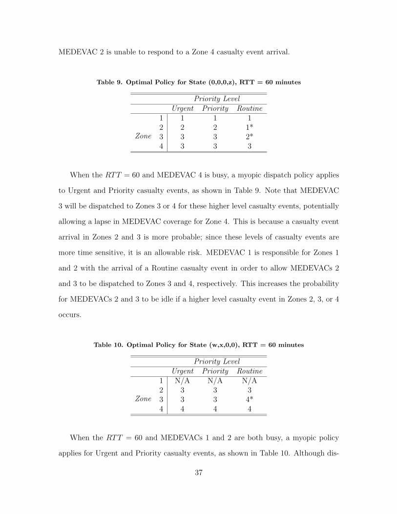
MEDEVAC 2 is unable to respond to a Zone 4 casualty event arrival.

Table 9. Optimal Policy for State (0,0,0,z), RTT = 60 minutes


Zone

1 1 1 12 2 2 1*3 3 3 2*4 3 3 3


to Urgent and Priority casualty events, as shown in Table 9. Note that MEDEVAC

3 will be dispatched to Zones 3 or 4 for these higher level casualty events, potentially

allowing a lapse in MEDEVAC coverage for Zone 4. This is because a casualty event

arrival in Zones 2 and 3 is more probable; since these levels of casualty events are

more time sensitive, it is an allowable risk. MEDEVAC 1 is responsible for Zones 1

and 2 with the arrival of a Routine casualty event in order to allow MEDEVACs 2

and 3 to be dispatched to Zones 3 and 4, respectively. This increases the probability

for MEDEVACs 2 and 3 to be idle if a higher level casualty event in Zones 2, 3, or 4

occurs.

Table 10. Optimal Policy for State (w,x,0,0), RTT = 60 minutes


Zone

1 N/A N/A N/A2 3 3 33 3 3 4*4 4 4 4

When the RTT = 60 and MEDEVACs 1 and 2 are both busy, a myopic policy

applies for Urgent and Priority casualty events, as shown in Table 10. Although dis-

37

patching MEDEVAC 3 to Zone 3 in this situation will potentially allow a casualty

event arrival in Zone 2 to have a lapse in MEDEVAC coverage, MEDEVAC 4 may

be unable to respond in time due to the further distance between Zones 3 and 4.

Therefore, despite the potential of missed coverage, it is better to respond as quickly

as possible with the closest MEDEVAC unit given an Urgent or Priority casualty

event. With the arrival of a Routine casualty event while MEDEVACs 1 and 2 are

busy, MEDEVAC 3 is reserved for Zone 2 arrivals only while MEDEVAC 4 will be

dispatched to Zones 3 and 4. Since this level of casualty event is not life-threatening,

it is better to reserve MEDEVAC 3 for Zone 2 alone, given the higher ratio of 9-

line MEDEVAC requests for Zone 2. Since MEDEVACs 1 and 2 are both busy and

MEDEVACs 3 and 4 are unable to respond to a casualty event in Zone 1, any ca-

sualty event that occurs in Zone 1 will not be supported with MEDEVAC capabilities.

Table 11. Optimal Policy for State (0,0,y,z), RTT = 60 minutes


Zone

1 1 1 12 2 2 1*3 2 2 24 N/A N/A N/A

When the RTT = 60 and MEDEVACs 3 and 4 are busy, the dispatch policy for

Urgent and Priority casualty events are myopic, as shown in Table 11. MEDEVAC

2 is responsible for both Zones 2 and 3 while MEDEVAC 1 is responsible for Zone 1

only. This policy allows the risk of a Zone 3 casualty event arrival to be unsupported

if MEDEVAC 2 is busy with a Zone 2 arrival. Although Zones 2 and 3 both have a

relatively high ratio of 9-line MEDEVAC request, it is more important that Urgent

and Priority casualties be responded to as quickly as possible. The dispatch policy

for a Routine casualty event is not myopic. Rather, MEDEVAC 1 is responsible for

38

both Zones 1 and 2. This is because this level of casualty event is not life-threatening

so it is more beneficial to reserve MEDEVAC 2 for Zone 3 arrivals or for future higher

level casualty events. Since MEDEVACs 3 and 4 are busy and MEDEVACs 1 and 2

are unable to respond to Zone 4, any casualty event occurring in Zone 4 will not be

supported with MEDEVAC capabilities.

Table 12. Optimal Policy for State (w,0,0,z), RTT = 60 minutes


Zone

1 2 2 22 2 2 23 3 3 2*4 3 3 3

When the RTT = 60 and MEDEVACs 1 and 4 are busy, a myopic dispatch policy

applies to Urgent and Priority casualty events, as shown in Table 12. However, in

the event of a Routine casualty event, MEDEVAC 3 is reserved while MEDEVAC

2 is responsible for Zones 1, 2, and 3. This is likely due to the distance to a Zone

4 casualty event and the low ratio of casualty event arrivals for Zone 1. With this

policy MEDEVAC 2 will provide MEDEVAC coverage for the first three zones if a

Routine casualty event occurs; this allows MEDEVAC 3 to be responsible for Zone

4 exclusively, reducing the potential for Zone 4 to have a lapse in MEDEVAC coverage.

Table 13. Optimal Policy for State (w,0,y,0), RTT = 60 minutes


Zone

1 2 2 22 2 2 23 2 4 44 4 4 4

39

When the RTT = 60 and MEDEVACs 1 and 3 are busy, a myopic dispatch pol-

icy applies for all priority classifications of casualty events, as shown in Table 13.

However, MEDEVAC 2 is responsible for Urgent casualty events in Zones 1, 2 and 3

and MEDEVAC 4 is responsible for Zone 4 only. This is because MEDEVAC 4 will

likely need to travel a further distance to Zone 3 from Zone 4 than MEDEVAC 2 will

from Zone 2. Since Urgent casualty events are extremely time sensitive, MEDEVAC

2 is responsible for Zone 3 despite the potential lapse in coverage for Zones 1 and 2

during a Zone 3 response. While still myopic, MEDEVAC 4 is responsible for both

Zones 3 and 4 while MEDEVAC 2 is responsible for Zones 1 and 2 for Priority and

Routine casualty events. Since these levels of casualty events are less time sensitive,

it is better to reserve MEDEVAC 2 for future higher level casualty events. Therefore

it is reasonable that MEDEVAC 2 is responsible for Zones 1 and 2 while MEDEVAC

4 is responsible for Zones 3 and 4.

Table 14. Optimal Policy for State (0,x,0,z), RTT = 60 minutes


Zone

1 1 1 12 1 1 13 3 3 34 3 3 3

Similar to Table 13, when the RTT = 60 MEDEVACs 2 and 4 are busy, a myopic

dispatch policy applies to all priority classifications of casualty events, as shown in

Table 14. This is due to the distance required for MEDEVACs 1 and 3 to respond

to each other’s mutually responsible zones, in this case only Zone 2. Although Zone

2 has a very high ratio of casualty event arrivals, Zone 1 has a relatively low ratio.

Likewise, Zone 4 has a lower ratio of casualty event arrivals, whereas the ratio of

casualty event arrivals for Zone 3 is relatively high. Given these ratios, it makes sense

40

that MEDEVAC 1 is responsible for Zones 1 and 2 while MEDEVAC 3 is responsible

for Zones 3 and 4.

Table 15. Optimal Policy for State (0,0,0,0), RTT = 90 minutes


Zone

1 1 1 12 2 2 1*3 3 3 34 4 4 4

Recall that only three optimal policies changed when the RTT = 90 rather than

60. When the RTT = 90 and all MEDEVAC units are idle, the dispatch policy is

myopic for Urgent and Priority casualty events, as shown in Table 15. When a Rou-

tine casualty event occurs, however, MEDEVAC 1 will be dispatched for any casualty

events in Zones 1 and 2 in order to reserve MEDEVAC 2 for any higher priority casu-

alty events. Unlike the policy for this state when the RTT = 60, as shown in Table 5,

MEDEVAC 3 is responsible for Zone 3 rather than MEDEVAC 4. This is because

MEDEVAC 4 is afforded more time when the RTT = 90, allowing it to respond to

Zone 3 if MEDEVAC 3 is busy when a casualty event arrives for Zone 3. This makes

it unnecessary to reserve MEDEVAC 3 for future higher level casualty events.

Table 16. Optimal Policy for State (w,x,0,0), RTT = 90 minutes


Zone

1 N/A N/A N/A2 3 3 33 3 4* 4*4 4 4 4

41

When the RTT = 90 and MEDEVACs 1 and 2 are busy, as shown in Table 16,

a myopic dispatch policy applies to Urgent casualty events as it does when the

RTT = 60. However, with an extra 30 minutes allowed for response time, MEDEVAC

4 has ample time to respond to Priority or Routine casualty events in Zone 3, allowing

MEDEVAC 3 to provide MEDEVAC coverage for Zone 2 only. This will reduce the

potential for a casualty in Zone 2 to be without MEDEVAC coverage, which is more

important given the high ratio of 9-line MEDEVAC request arrivals for Zone 2. Since

MEDEVACs 1 and 2 are both busy and MEDEVACs 3 and 4 are unable to respond

to a casualty event in Zone 1, any casualty event that occurs in Zone 1 will not be

supported with MEDEVAC capabilities.

Table 17. Optimal Policy for State (0,0,y,z), RTT = 90 minutes


Zone

1 1 1 12 2 1* 1*3 2 2 24 N/A N/A N/A

When the RTT = 90 and MEDEVACs 3 and 4 are busy, a myopic dispatch

policy applies to Urgent casualty events, as shown in Table 17, as is the case when

the RTT = 60, depicted in Table 11. However, given an additional 30 minutes for

responding, the dispatch policy is not myopic for Priority or Routine casualty events.

Instead, MEDEVAC 1 is responsible for Zones 1 and 2 while MEDEVAC 2 is only

responsible for Zone 3. This allows MEDEVAC 2 to be reserved in order to provide

MEDEVAC coverage for Zone 3, since Zone 3 cannot be supported by any other

MEDEVAC unit. Given that Zones 2 and 3 have a relatively high casualty event

arrival ratio, it is better to dispatch different MEDEVAC units for these zones since

they are not supported by any other unit given a lower priority casualty event. Since

42

MEDEVACs 3 and 4 are busy and MEDEVAC 2 is unable to respond to Zone 4, any

casualty event occurring in Zone 4 will not be supported with MEDEVAC capabilities.

5.3 MEDEVAC System Under Different Scenarios and Policies

In order to further examine the results of our model of the MEDEVAC system

when supporting combat operations, we analyze three different combat scenarios. We

continue to use current operations in support of OEF in southern Afghanistan as the

basis of these scenarios, but change several conditions within the combat environment.

The first scenario we analyze is the base case that we’ve described in previous sections.

Recall that we have looked at steady state stability operations with a relatively low

9-line MEDEVAC arrival rate of λ = 1327

, modest yet accurate parameters for armed

escort delays within the system, with E = 30 minutes, θ1 = 0.31, and θ2 = 0.04, and

a relatively low rate of Urgent and Priority level casualties and casualty events, with

q1 = 0.11, q2 = 0.12, p1 = 0.1587, p2 = 0.1574.

The second scenario we analyze keeps the same parameters established in the base

case with the exception of the armed escort delay parameters. This scenario reflects

an operational environment with an increase threat level, thereby requiring a higher

ratio of armed escorts per MEDEVAC mission. We consider this scenario with an

increased armed escort delay, E, of 30 minutes, an increased chance of a MEDEVAC

mission requiring an armed escort, θ1 = 0.60, and an increased ratio of MEDEVAC

missions that are delayed due to issues with the armed escort, θ2 = 0.30.

The third scenario we analyze considers a period of time when Coalition Forces

experience a heightened level of enemy activity and therefore an increased number of

casualty events. Stability operations in support of OEF during periods of peak enemy

activity time periods, historically during the summer, will cause several parameters

of our model to increase. In order to gain a realistic perspective of the effect that the

43

summer fighting season has on the number of casualty events, we examine the KIA

statistics found on icasualties.org [22]. According to the statistics, operations during

2010 proved to be the most casualty producing, with the summer months accruing

the most KIAs, as expected. As shown in Figure 4, Coalition Forces experienced the

highest number of KIAs during the months of June through August of 2010, with an

average of 90 KIAs per month.

Figure 4. Number of Coalition Forces KIA in 2010

Since we are interested in casualty events, which also include the number of WIAs,

it is necessary to consider the total number of casualties, both KIAs and WIAs, for

our model. According to Gartner [18], the ratio of KIA to WIA in OEF is 0.12.

By straight calculation we determine that an average of 750 casualties occurred each

month during the summer of 2010, which yields an average of 581 casualty events per

month given that the probabilities of there being one, two, three, and four casualties

44

per casualty event is α = (0.574, 0.36, 0.05, 0.016). Therefore, we determine that the

casualty event arrival rate during a period of heightened enemy activity is λ = 174

.

We also use the increased armed escort delay parameters of E = 30, θ1 = 0.60, and

θ2 = 0.30. During a time of increased attacks against Coalition Forces we also expect

a higher ratio of Urgent and Priority casualties. It is reasonable to assume that the

ratio of Urgent casualties, q1, will increase from 0.11 to 0.25, and the ratio of Priority

casualties, q2, will increase from 0.12 to 0.28, and the ratio of Routine casualties, q3,

to decrease from 0.77 to 0.47. These ratios are obtained arbitrarily as the data is not

readily available. This will cause the ratio of Urgent casualty events, p1, to increase

from 0.1587 to 0.341, the ratio of Priority casualty events, p2, to increase from 0.1574

to 0.304, and the ratio of Routine casualty events, p3, to decrease from 0.6839 to

0.355.

For each of these scenarios, we examine three different policies: an optimal policy,

a myopic policy, and an intra-zone policy. Each policy is a valid decision-making tool

when different constraints or directives affect the combat environment. For example,

an optimal policy, the policy that this paper focuses on and develops, can be used

given the data has been analyzed enough for the specific AO. Moreover, this policy

requires the BCTs responsible for each zone to cooperate with each other in terms of

co-using MEDEVAC assets.

A myopic policy might be used in the decision-making process of dispatching

MEDEVAC units if the response time, Rij, is defined differently and it is more crucial

to reach the casualty quickly than it is to transport the casualty to the MTF quickly.

This difference may be realized with the recent blood transfusion capability that US

MEDEVAC units currently possess. Recall that our response time, Rij, is based on

the fact that blood loss is the leading cause of death on the battlefield and therefore

transporting the casualty to a MTF in order to stop the blood loss and receive a blood

45

transfusion is more important than simply reaching the casualty quickly. However,

if a blood transfusion can be administered at the casualty site or enroute to the

MTF, the response time, Rij, will most likely be defined as the time it takes to

reach the casualty site after receipt of the 9-line MEDEVAC request, as opposed

to our definition. In this case, a myopic policy may perform well with dispatching

MEDEVAC units to casualty events. Therefore, it is important to compare a myopic

policy to other policies.

Lastly, an intra-zone policy may be implemented depending on the operating

environment. Recall that an intra-zone policy only allows a MEDEVAC unit to service

casualty events that occur within its respective zone. This policy may be forced upon

the MEDEVAC system if multiple nations or services have adjacent AORs but do not

operate closely with each other and therefore do not share MEDEVAC capabilities.

While each policy is better than simply assuming which MEDEVAC unit is the

best to dispatch to a casualty event, some policies perform better than others in the

long run. It is important to examine the operating environment when implementing

one policy over another. To illustrate this, we examine each of the three policies when

applied to the three different scenarios previously described.

5.3.1 Performance of Different Policies Applied to Stability Opera-

tions (Base Case).

We first examine how each of the three policies previously described will perform

under the circumstances of the base case examined in the majority of this paper.

Recall the input parameters and their respective values; with these values we analyze

the MEDEVAC system with a RTT of 60 minutes. Figure 5 portrays the expected

utility for each zone when the three different policies are implemented. It also portrays

the probability that a MEDEVAC unit will be busy for each policy.

46

Figure 5. Stability Operations (Base Case) RTT = 60

The expected utility for Zone 1 is nearly non-existent. This is to be expected since

the proportion of casualty events in Zone 1 is φ1 = 0.004; a change in the operational

environment will affect this whereas a difference in policy or other parameters will

not. We examine a change in φ1 in the subsequent section. The expected utility

of Zones 2 and 3, however, are far greater when an optimal policy is implemented,

with a total of 0.177; this is compared to a total of 0.120 when a myopic policy is

implemented. An intra-zone policy is least preferred with a total expected utility for

Zones 2 and 3 of 0.039. The expected utility for Zone 4 is nearly identical for optimal

and myopic policies, with 0.0132 and 0.0133, respectively. Again, an intra-zone policy

is least preferred with 0.0031. Overall, the total expected zone utilities for optimal,

myopic, and intra-zone policies are 0.191, 0.134, and 0.043, respectively.

When the probabilities of each MEDEVAC being busy are examined, we see no-

table differences. When an optimal policy is implemented, we see that MEDEVACs

1 and 4 are busy far more often with probabilities of 0.0561 and 0.0515, respectively,

than when myopic or intra-zone policies are implemented, with probabilities of 0.0026

and 0.0077, respectively, with a myopic policy and 0.0001 and 0.0023, respectively,

with an intra-zone policy. This is because MEDEVACs 2 and 3 are often rationed

47

when using an optimal policy in order to reserve MEDEVACs 2 and 3 for future

higher priority level casualty events. Recall that Zones 2 and 3 have a higher ra-

tio of casualty event arrivals and therefore require MEDEVAC services more often.

When a myopic policy is implemented in this scenario, MEDEVAC 2 is dispatched

far more often than MEDEVAC 1 with a busy probability of 0.0463 compared to

0.0026, respectively, causing a potential lapse in coverage for a casualty event in Zone

2 when RTT = 60. Consequently, MEDEVAC 1 is under-utilized with a myopic

policy. Proportionally, the same outcome exists for Zones 3 and 4, where MEDEVAC

4 is under-utilized when a myopic policy is used in comparison to when an optimal

policy is used. An intra-zone policy simply reflects the proportion of casualty events

in each zone; this policy will most likely prove to be inefficient under circumstances

of higher threat, as well.

When the NATO RTT standard of 90 minutes is applied for the same scenario,

as shown in Figure 6, we see similar results for the zone utilities but some notable

differences with the expected usage of MEDEVAC units.

Figure 6. Stability Operations (Base Case) RTT = 90

The expected utilities for Zones 1, 2 and 4 are nearly identical, proportionally,

when compared to the scenario with a RTT of 60 minutes; as expected, the utilities

48

for each of these zones increases slightly due to higher mission utilities when the

MEDEVAC units have 30 additional minutes to respond to a casualty event. The

utility for Zone 3, however, is nearly the same when an optimal or myopic policy

is applied, 0.0536 and 0.0505, respectively. Note that with a RTT of 90 minutes,

the utility for Zone 3 decreases when using an optimal policy, which is not intuitive

at first. One would most likely expect to see the zone utility to increase for this

zone as well. However, by looking at the changes in optimal policies when the RTT

= 90 rather than 60, we see that MEDEVAC 3 is dispatched to Zone 3 for Routine

casualty events instead of MEDEVAC 4 when the system is in state (0,0,0,0). We also

see that MEDEVAC 4 is dispatched to Zone 3 for Priority casualty events instead of

MEDEVAC 3 when the system is in state (w,x,0,0). The unrewarded Routine casualty

events that MEDEVAC 3 responds to in Zone 3 may account for the decrease in zone

utility. The total zone utility when an optimal policy is applied increases to 0.194

when the RTT = 90 and increases to 0.154 and 0.049 when myopic or intra-zone

policies applied, respectively.

When an optimal policy is applied, the probabilities of each MEDEVAC unit

being busy differ substantially when the RTT is 90 minutes rather than 60 minutes.

However, the expected MEDEVAC utilizations remained the same when either myopic

or intra-zone policies are applied. Therefore we focus on the differences when an

optimal policy is being used. When this is the case, the probabilities are very similar

for MEDEVACs 1 and 2 regardless of the RTT change, but are quite different for

MEDEVACs 3 and 4. MEDEVAC 4 is utilized much less when the RTT is 90 minutes,

whereas MEDEVAC 3 is utilized much more. This is because the optimal policies

change for states (0,0,0,0) and (w,x,0,0) when the RTT = 90. Since MEDEVAC 3

is dispatched to Zone 3 for Routine casualty events rather than MEDEVAC 4 and

49

Routine casualty events account for 77% of the MEDEVAC missions, the decrease in

usage of MEDEVAC 4 and increase in usage of MEDEVAC 3 is intuitive.

5.3.2 Stability Operations With Increased Armed Escort Delay Pa-

rameters.

A change that may occur with a heightened level of enemy activity, such as dur-

ing the summer of 2010, is the number of times troops will be in direct contact with

the enemy, thereby requiring the support of Air Weapons Teams or Scout Weapons

Teams. These are the same helicopter teams that provide an armed escort to MEDE-

VAC units. If troops are in contact with the enemy more often there will be a higher

demand for these helicopter teams, resulting in a higher armed escort delay within

our model. We examine what would occur within our model if the armed escort delay,

E, is increased from 10 to 30 minutes. We also increase the chance of requiring an

armed escort, θ1, from 31% to 60%. Of those MEDEVAC missions that require an

armed escort, we increase the chance of a delay due to issues with the escort air-

craft, θ2, from 4% to 30%. These different percentages are arbitrarily derived but are

reasonable given a high operational tempo during heightened levels of enemy activity.

Even with such a large increase in the parameters for the armed escort, only two

states experience a change in their optimal policies: states (0,0,y,0) and (w,0,0,z). For

state (0,0,y,0), the additional armed escort delay causes MEDEVAC 2 to be reserved

when a Routine casualty event arrives in Zone 3, dispatching MEDEVAC 4 in its

place. This will allow MEDEVAC 2 to respond to future higher level casualty events

instead, as shown in Table 18.

With an increased armed escort delay, the optimal policy for state (w,0,0,z) no

longer dispatches MEDEVAC 2 to Zone 3 for a Routine casualty event, but instead

50

Table 18. Optimal Policy for State (0,0,y,0), RTT = 60 minutes, Increased AE delay


Zone

1 1 1 12 2 2 1*3 2 2 44 4 4 4

becomes myopic, thereby dispatching MEDEVAC 3, as shown in Table 19. This

change allows MEDEVAC 2 to respond to Zones 1 and 2 only, regardless of the ca-

sualty event priority classification.

Table 19. Optimal Policy for State (w,0,0,z), RTT = 60 minutes, Increased AE delay


Zone

1 2 2 22 2 2 23 3 3 34 3 3 3

When the optimal policy is compared to the myopic and intra-zone policies with

a RTT of 60 minutes, as shown in Figure 7, we find that the zone utility is identical

when using an optimal policy. The zone utilities are nearly the same when using

myopic or intra-zone policies, with slight increases for both. The total zone utilities

for optimal, myopic, and intra-zone policies are 0.191, 0.139, and 0.045, respectively.

In regards to the expected usage of each MEDEVAC, we see little change between

the different policies used. Intuitively, each MEDEVAC has a slightly higher prob-

ability of being busy regardless of which policy is applied to the system. Note that

MEDEVACs 2 and 3 continue to be used much less often than MEDEVACs 1 and 4

in order to reserve them for higher casualty event arrivals in Zones 2 and 3.

51

Figure 7. Stability Operations With Increased Armed Escort Delay Parameters, RTT= 60

When the RTT is changed from 60 to 90 minutes, there is a noticeable increase in

the zone utilities for each of the three different policies, as shown in Figure 8. Overall,

however, the optimal policy shows the largest improvement over it’s already larger

total zone utility. Specifically, there is an increase of 0.0495 in zone utility when an

optimal policy is applied, with a total zone utility of 0.241; there is an increase of

0.0284 in zone utility when a myopic policy is applied, with a total zone utility of

0.167; lastly, there is an increase of 0.0087 in zone utility when an intra-zone policy is

applied, with a total zone utility of 0.0532. When the RTT = 90, there is no change

to the probabilities of each MEDEVAC being busy regardless of the policy method

applied.

5.3.3 Stability Operations During Heightened Enemy Activity.

Our base case scenario involves steady state stability operations with a relatively

low occurrence of enemy activity compared to conflicts with more severe casualty

events. Therefore, it is imperative that we apply our model to a more hostile environ-

ment. As previously described, we look at a period during OEF when enemy activity

was at its highest level, the summer months of 2010.

52

Figure 8. Stability Operations With Increased Armed Escort Delay Parameters, RTT= 90

Changing the parameters within our model to reflect the heightened level of enemy

activity experienced in the summer of 2010, we see that, with a RTT of 60 minutes,

zone utilities for each policy method increased by a large margin. The total zone

utilities when an optimal, myopic, or intra-zone policy is applied to a MEDEVAC

system with increased enemy activity are 1.28, 0.717, and 0.265, respectively. How-

ever, as Figure 9 depicts, the zone utilities increased proportionally; therefore, the

relative performance of each policy method does not change with increased casualty

event arrivals when compared.

Intuitively, the probability of each MEDEVAC unit increased by a large margin

as well. MEDEVACs 1 and 4 continue to be used more often than MEDEVACs 2 and

3, but with a heightened level of enemy activity, MEDEVACs 2 and 3 are not able

to be rationed as often as they were in the first two scenarios. MEDEVAC 3 is the

least busy, however, being used almost half as much as the other three MEDEVACs.

As with the other scenarios, the myopic policy dispatches MEDEVACs 2 and 3 the

most while under-utilizing MEDEVACs 1 and 4.

When the RTT is increased to 90 minutes, we find that the zone utilities for each

policy method increase, as shown in Figure 10. This is intuitive since the mission

53

Figure 9. Stability Operations With Increased Enemy Activity, RTT = 60

utilities also increase. However, the proportion of increase is quite different under

the heightened enemy activity parameters. By applying an optimal policy, little

improvement is realized with only a 3.7% gain, from 1.28 to 1.33. When myopic

or intra-zone policies are applied, however, nearly the same increase is achieved as

when the RTT was changed from 60 to 90 minutes in the large AE delay scenario;

an increase of 0.148 in zone utility, from 0.717 to 0.865, for a myopic policy, and an

increase of 0.052 in zone utility, from 0.265 to 0.317, for an intra-zone policy.

The probabilities of MEDEVACs 1, 2 and 3 being busy in a system with heightened

enemy activity and a RTT of 90 minutes are very similar, with MEDEVAC 1 being

used the most and MEDEVACs 2 and 3 being used less. Unexpectedly, however, while

MEDEVAC 4 is used in the same fashion as in the other scenarios when a myopic

or intra-zone policy method is applied, its use differs greatly when an optimal policy

method is applied. MEDEVAC 4 is the least used unit when an optimal policy is

applied, indicating that MEDEVACs 2 and 3 are not rationed as often as they are in

the other scenarios or when the RTT = 60.

54

Figure 10. Stability Operations With Increased Enemy Activity, RTT = 90

5.4 Sensitivity Analysis

5.4.1 Change in Arrival Rate.

As portrayed in the example of a combat environment during periods of time with

elevated enemy activity, the arrival rate is a parameter in our model that is quite

sensitive. For example, if we use our model in an operating environment where a

casualty event occurs once every 30 minutes, λ = 130

, but all other parameters remain

unchanged, our system of only one MEDEVAC unit per zone could be expected to

be busy at all times since the service rate is much less, sometimes by half, the arrival

rate. However, recall that since our system operates with an inter and intra-zone

policy, MEDEVAC units from other zones are able to respond to casualty events in

their own zone as well as zones adjacent to them. This allows greater flexibility with

an increased arrival rate. We show the effects of a busier MEDEVAC system given

a higher arrival rate in the previous section; however, to examine how sensitive this

parameter is, we look at changes in the optimal policy throughout a range of different

arrival rates. We examine these changes when the RTT = 60 only.

55

When λ = 130

, six states experience at least one change in their optimal policies

while they remain the same for the other four states. When all MEDEVAC units are

idle, state (0,0,0,0), MEDEVAC 3 is dispatched to Zone 3 for Routine casualty events

instead of MEDEVAC 4. When MEDEVAC 3 is busy, state (0,0,y,0), MEDEVAC 4

is dispatched to Zone 3 instead of MEDEVAC 2 for Priority and Routine casualty

events. When MEDEVAC 4 is busy, state (0,0,0,z), MEDEVAC 3 is dispatched to

Zone 3 for Routine casualty events instead of MEDEVAC 2. When MEDEVACs 3

and 4 are busy, state (0,0,y,z), MEDEVAC 1 is dispatched to Zone 2 for Priority

casualty events instead of MEDEVAC 2. When MEDEVACs 1 and 4 are busy, state

(w,0,0,z), MEDEVAC 3 is dispatched to Zone 3 for Routine casualty events instead of

MEDEVAC 2. Lastly, when MEDEVACS 1 and 2 are busy, state (w,x,0,0), MEDE-

VAC 4 is dispatched to Zone 3 for Priority casualty events instead of MEDEVAC 3.

As shown in Figure 11, when the casualty event arrival rate is increased to λ = 130

,

zone utilities are dramatically increased. This is intuitive since many more casualty

events are serviced. Moreover, a large increase in each MEDEVAC’s busy probabili-

ties is seen. The pattern for these probabilities remains the same when a myopic or

intra-zone policy method is applied to the system, but differs when an optimal policy

method is applied. The most notable difference is that, proportionally, MEDEVAC

4 is used less than before while MEDEVAC 3 is used more often.

We focus on the state when every MEDEVAC unit is idle, state (0,0,0,0), as

this state is one whose optimal policy changes with a busier system. When each

MEDEVAC unit is idle within a busier system, a change in policy occurs when there

is a Routine casualty event arrival. With the original arrival rate of one casualty event

every 327 minutes, the policy for a Routine casualty event is to dispatch MEDEVAC

4 to Zone 3 in order to reserve MEDEVAC 3 for future higher level casualty events,

as shown in Table 5. However, the policy for this state requires MEDEVAC 3 to

56

Figure 11. Change in Arrival Rate, λ = 130 , RTT = 60

respond to a Routine casualty event in Zone 3 when the arrival rate is one casualty

per 30 minutes, as shown in Table 20.

Table 20. Optimal Policy for State (0,0,0,0), RTT = 60 minutes, λ = 130


Zone

1 1 1 12 2 2 1*3 3 3 34 4 4 4

The optimal policy for this state continues to change depending on the arrival

rate. For example, when one 9-line MEDEVAC request arrives every minute, λ = 11,

the dispatch policy for Urgent casualty events is myopic whereas Priority and Routine

casualty events only dispatch MEDEVACs 1 and 4, thereby reserving MEDEVACs 2

and 3 for higher level casualty events, as shown in Table 21.

When 9-line MEDEVAC requests arrive once every two through eight minutes,

λ = 12

to 18, the optimal policy remains the same for Urgent and Routine casualty

events, but changes for Priority casualty events. Priority casualty events require

57

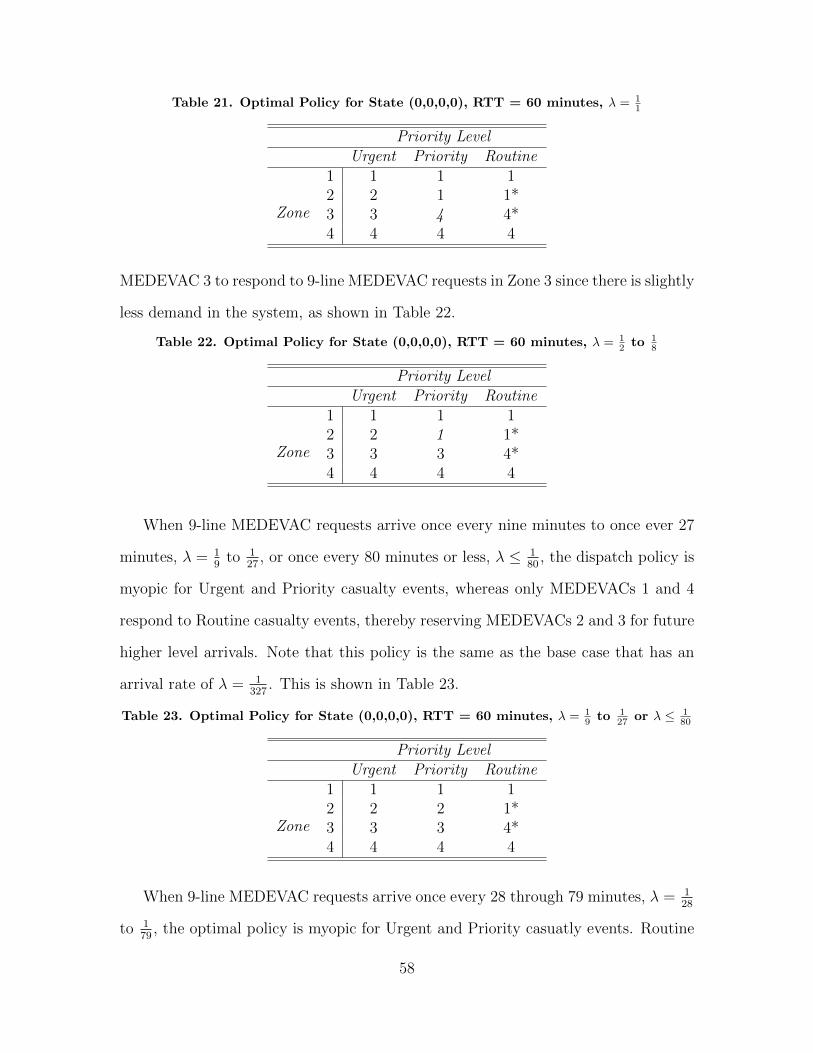
Table 21. Optimal Policy for State (0,0,0,0), RTT = 60 minutes, λ = 11


Zone

1 1 1 12 2 1 1*3 3 4 4*4 4 4 4

MEDEVAC 3 to respond to 9-line MEDEVAC requests in Zone 3 since there is slightly

less demand in the system, as shown in Table 22.

Table 22. Optimal Policy for State (0,0,0,0), RTT = 60 minutes, λ = 12 to 1

8


Zone

1 1 1 12 2 1 1*3 3 3 4*4 4 4 4

When 9-line MEDEVAC requests arrive once every nine minutes to once ever 27

minutes, λ = 19

to 127

, or once every 80 minutes or less, λ ≤ 180

, the dispatch policy is

myopic for Urgent and Priority casualty events, whereas only MEDEVACs 1 and 4

respond to Routine casualty events, thereby reserving MEDEVACs 2 and 3 for future

higher level arrivals. Note that this policy is the same as the base case that has an

arrival rate of λ = 1327

. This is shown in Table 23.


27 or λ ≤ 180


Zone

1 1 1 12 2 2 1*3 3 3 4*4 4 4 4

When 9-line MEDEVAC requests arrive once every 28 through 79 minutes, λ = 128

to 179

, the optimal policy is myopic for Urgent and Priority casuatly events. Routine

58

casualty events, however, dispatch MEDEVAC 3 to Zone 3 since there is even less

demand in the system. This is shown in Table 24.


79


Zone

1 1 1 12 2 2 1*3 3 3 34 4 4 4

5.4.2 Change in φi, the proportion of 9-line MEDEVAC requests in

demand Zone i.

We also consider changing the casualty zone ratio, φi = 0.004, 0.585, 0.338, 0.073;

since Zones 1 and 4 have relatively low ratios we focus on increasing φ1 and φ4 sepa-

rately while keeping the proportionality of the other zone ratios intact. For example,

by changing φ1 to 0.35, φ2 becomes 0.382, φ3 becomes 0.220, and φ4 becomes 0.048.

By increasing the proportion of casualty events in Zone 1, we see in Figure 12 that

the zone utility for Zone 1 increases drastically while the utilities for the other three

zones decrease. This is quite intuitive since servicing more MEDEVAC missions will

yield a higher utility; therefore, the more casualty events that occur in a particular

zone, the more potential utility that zone will have. Note that the probability that

MEDEVAC 1 will be busy decreases greatly while the probability that MEDEVAC

2 is busy increases. This indicates that when φ = 0.35, MEDEVAC 1 is rationed for

higher level casualty events.

Once again we look at the state when all MEDEVAC units are idle, state (0,0,0,0).

We know from Table 5 that, under the base case parameters, a myopic policy applies

to Urgent and Priority casualty events while MEDEVAC 1 is dispatched to Zones 1

59

Figure 12. Change in Proportion of 9-line MEDEVAC requests for Zone i, φ1 = 0.35,RTT = 60

and 2 for a Routine casualty event and MEDEVAC 4 is dispatched to Zones 3 and

4. However, when the casualty zone ratio is increased for Zone 1 so that φ1 ≥ .22,

MEDEVAC 2 is dispatched to Zone 2 instead of MEDEVAC 1, as shown in Table 25.

Note that MEDEVAC 4 is still dispatched to Zones 3 and 4 for Routine casualty

events in order to reserve MEDEVAC 3 for future higher priority casualty events.

Table 25. Optimal Policy for State (0,0,0,0), RTT = 60 minutes, φ1 = 0.22


Zone

1 1 1 12 2 2 23 3 3 4*4 4 4 4

We also look at a state when one MEDEVAC unit is busy. The optimal policy

for the system when one MEDEVAC unit is busy is relatively identical whether the

busy MEDEVAC is 1, 2, 3, or 4. In each of these states the optimal policy is myopic

for Urgent and Priority casualty events whereas Routine events require one or more

MEDEVAC unit to be reserved for future casualty events. Therefore, examining

state (w,0,0,0), we know from Table 6 that a myopic policy applies to Urgent and

60

Priority casualty events, whereas only MEDEVACs 2 and 4 are dispatched for Routine

casualty events, thereby reserving MEDEVAC 3 for future higher priority casualty

events. However, when φ1 ≥ 0.03, MEDEVAC 2 is responsible for Zone 1 only when

MEDEVAC 3 is responsible for Zone 2 for Routine casualty events while the system

is in state (w,0,0,0), as shown in Table 26.

Table 26. Optimal Policy for State (w,0,0,0), RTT = 60 minutes, φ1 = 0.03


Zone

1 2 2 22 2 2 3*3 3 3 4*4 4 4 4

When changing φ4 we look at the system when all MEDEVAC units are idle, state

(0,0,0,0). We know from Table 5 that MEDEVAC 4 is only responsible for Zone 4 for

Urgent and Priority casualty events, but is dispatched to Zones 3 and 4 for Routine

casualty events. However, if φ4 is increased to 0.078, MEDEVAC 3 will be dispatched

to Zone 3 for Routine casualty events in order to allow MEDEVAC 4 to respond to

Zone 4 only, as shown in Table 27. Note that MEDEVAC 1 is still responsible for

Zones 1 and 2 in order to reserve MEDEVAC 2 for future higher priority casualty

events.



Zone

1 1 1 12 2 2 1*3 3 3 34 4 4 4

61

Moreover, if φ4 is increased to 0.12 then the system will dispatch MEDEVAC 3 to

Zones 3 and 4 for Routine casualty events, thereby reserving MEDEVAC 4 for future

higher priority casualty events, as shown in Table 28.



Zone

1 1 1 12 2 2 1*3 3 3 34 4 4 3*

Lastly, we look at the system when one MEDEVAC unit is busy, in this case when

MEDEVAC 3 is busy, state (0,0,y,0). As shown in Table 8, a myopic dispatch policy

applies to Urgent and Priority casualty events. For Routine casualty events, however,

MEDEVAC 1 is responsible for both Zones 1 and 2. When φ4 is decreased to 0.065,

only MEDEVACs 1 and 4 are dispatched, reserving MEDEVAC 2 for future higher

priority casualty events, as shown in Table 29.

Table 29. Optimal Policy for State (0,0,y,0), RTT = 60 minutes, φ1 = 0.065


Zone

1 1 1 12 2 2 1*3 2 2 4*4 2* 2* 4

62

VI. Conclusions

Discussion and Results

The nature of the MEDEVAC mission is one of urgency; therefore little time is af-

forded to the decision maker when a 9-line MEDEVAC request is received in regards

to what MEDEVAC unit should be dispatched. An instinctive reaction is to dispatch

the nearest MEDEVAC unit in order to respond to the casualty event as soon as

possible. This follows the logic of a myopic policy. However, this can result in grave

consequences if a MEDEVAC unit is dispatched to a low priority casualty event and

is therefore busy when a higher priority casualty event occurs in that unit’s zone.

Rapid blood loss on the battlefield is the leading cause of death according to current

statistics, and providing rapid medical support is essential to preserving the lives of

our soldiers. Losing a soldier to a gunshot wound or improvised explosive device be-

cause the nearest MEDEVAC unit is busy servicing a Routine casualty event such as

a broken leg is unacceptable. Our model proves to be useful by providing a decision

rule that dispatches the most appropriate MEDEVAC unit to casualty events and po-

tentially rations a closer, and sometimes more intuitive, MEDEVAC unit for future

casualty events that may be more time sensitive. To complicate the decision-making

process, situations with a high threat level require armed helicopters to escort the

MEDEVAC unit to the casualty site, creating a potential delay in the response time.

We use a computational example based on the current operational environment in

Afghanistan to apply a MDP model using our value iteration dynamic programming

algorithm to develop an optimal policy for dispatching MEDEVAC units that may

save soldiers’ lives.

Since we know the location and priority level of each casualty event with the receipt

of a 9-line MEDEVAC request, we determine which MEDEVAC unit to dispatch in

order to maximize the steady-state system utility. The utility gained from servicing a

63

specific request depends on the number of casualties, the priority class of the casualty

event, and the location of both the servicing MEDEVAC unit and casualty site. The

location of the casualty site informs us on the dispatch options while the priority level

informs us on which MEDEVAC unit to dispatch.

Results indicate that a myopic policy is not always the best method to use for

quickly dispatching MEDEVAC units under differing threat conditions while conduct-

ing combat operations under a variety of different parameters. Although a myopic

policy performs better than an intra-zone policy, neither of these policies produce a

higher zone utility than the optimal policy method does throughout several parameter

changes and scenario alterations.

Analysis of the results indicate that when applying an optimal policy to a MEDE-

VAC system, the MEDEVAC that is dispatched in response to a 9-line MEDEVAC

request is highly dependent upon the proportion of casualty events per zone. From

studying our computational example, with a system that has a relatively low propor-

tion of casualty events in Zones 1 and 4, MEDEVACs 1 and 4 are used as often as

possible to respond to casualty events not only in their respective zones but also to

casualty events in Zones 2 and 3, respectively. This enables MEDEVACs 2 and 3 to

be reserved for only the higher level casualty events. This reduces the potential for

a MEDEVAC unit being busy servicing a Routine casualty event when an Urgent or

Priority casualty event arrives in its own respective zone.

Another parameter that the optimal policy method is dependent upon is the

casualty event arrival rate, λ. When this parameter is changed to a relatively high

rate, λ = 130

, the optimal policy changed in six of the 10 possible states within our

computational example. On the contrary, the armed escort delay is not as sensitive

as expected. While an increased delay produces lower zone utilities, it only changes

the optimal policy for two of the 10 states in our computational example.

64

Analyzing the results of our model also reveals that the myopic policy follows

the same dispatch pattern with each parameter alteration. While this policy method

produces different zone utilities and probabilities of each MEDEVAC being busy,

these changes are only reflective of the increased or decreased ratio of casualty events

per zone, regardless of their urgency. MEDEVACs 2 and 3 are consistently busy

while MEDEVACs 1 and 4 are under-utilized; this is because a myopic policy does

not consider rationing MEDEVAC units whose zones are expected to receive urgent or

priority casualty event arrivals more often than other zones. These factors consistently

produce a lower zone utility than a system using an optimal policy does.

Although a myopic policy proves to be inferior to an optimal policy, an intra-zone

policy is inferior to both. An intra-zone policy simply dispatches MEDEVAC units

when a casualty event occurs in their respective zones, giving no consideration to the

parameters within our model. No decision is required when deciding which MEDE-

VAC unit to dispatch, and many casualty events are likely not serviced when this

policy is applied, resulting in a total zone utility for each scenario examined that is

dramatically less than the other two policy methods.

Potential Future Research

While our model is useful, it also has several limitations as a number of aspects are

not examined. For example, we do not allow MEDEVAC units to respond to casualty

events until they return to their original staging location, although realistically a

MEDEVAC unit is able to be diverted to such missions given it has the necessary fuel

and equipment. This will certainly reduce the response time for many casualty events

given the 9-line MEDEVAC request is received shortly after a nearby MEDEVAC unit

has unloaded its casualties. Also, future research could examine the probabilities the

65

system has to be in each state in order to determine how often a lapse in coverage

occurs.

We also do not consider that a response time under 60 or 90 minutes could yield a

greater utility for Urgent casualty events given that a proportion of Urgent casualties

will not survive under the US or NATO standard RTTs, but may survive if the

mission was completed in less time. Moreover, we do not allow MEDEVAC units

to be placed in a queue; if this was possible, MEDEVAC units could be dispatched

to casualty event sites from nearby MTFs directly after unloading casualties from

the prior mission. Other than receiving no utility, our model does not capture the

negative effect of casualty events not provided with MEDEVAC support, thereby

using non-standard CASEVAC either by ground or air; a queuing system may provide

an otherwise unsupported casualty with crucial medical aid in a more timely manner.

Another possibility for future research involves basing the priority level of the

casualty event on the zone from which the event originates. For example, the propor-

tion of Urgent casualty events may be much greater in Zone 2 than in Zone 1, and

those probabilities could be incorporated within the model. Resource emplacement

could encompass this aspect of the MEDEVAC system. Our model does not consider

resource emplacement such as forward positioning MEDEVAC units in areas histor-

ically likely to receive 9-line MEDEVAC requests, specifically Urgent requests. By

changing a MEDEVAC unit’s staging location based on current data, the response

time could be reduced by a great enough margin to save lives.

Lastly, our model does not incorporate the recent MEDEVAC capability of pro-

viding blood transfusions enroute to the MTF. Recall that our response time, the

time required to transport a casualty from receipt of the 9-line MEDEVAC request to

an appropriate MTF, is based on the fact that blood loss is the primary cause of death

in a combat environment. If this new capability is incorporated into our model, the

66

response time parameters will change. Similarly, further examination could consider

survival probabilities for MEDEVAC units providing different medical capabilities;

for example, MEDEVAC units typically have flight medics on board, but on occasion

will have a physician’s assistant or surgeon. These additional assets would likely in-

crease the casualty survival rate. While our model is thorough in many aspects there

is room for improvement, and all of these limitations should be examined in future

research.

67

Appendix: Table of Notation

D = Total dispatching time; the amount of time required between the receipt of the

9-line MEDEVAC request and the MEDEVAC departure.

T c = The amount of time it takes for the MEDEVAC unit to travel from its staging

area to the casualty site.

E = The amount of time an armed escort delays the MEDEVAC unit.

θ1 = The chance of a MEDEVAC mission requiring an armed escort.

θ2 = The ratio of MEDEVAC missions requiring an armed escort that are delayed

due to issues with the escort aircraft.

Lc = The amount of time the MEDEVAC unit spends at the casualty site in order

to begin initial treatment and load the casualty onto the helicopter.

Tm = The amount of time it takes for the MEDEVAC unit to travel from the casualty

site to the nearest appropriate MTF.

Um = The amount of time it takes for the MEDEVAC crew to unload the patient at

the MTF.

T s = The amount of time it takes the MEDEVAC unit to travel from the MTF back

to its original staging area.

Rij = Total response time for MEDEVAC j to respond to a casualty event in Zone

i and transport the casualty to the nearest appropriate MTF; This is defined as the

sum of the dispatch time D, travel time to the casualty site T c, potential armed escort

delay E, the load time at the casualty site Lc, travel time to the appropriate medical

facility Tm, and the unload time at the medical treatment facility Um.

Vij = Total service time for MEDEVAC j to respond to a casualty event in Zone

i, transport the casualty to the nearest appropriate MTF and return to its original

staging area; This is defined as Rij + T s.

λ = 9-line MEDEVAC request arrival rate to the entire system.

68

d = Total number of demand zones.

m = Total number of MEDEVAC units.

φi = Proportion of 9-line MEDEVAC requests from demand Zone i such that:n∑i=1

φi =

1.

pk = Proportion of priority k 9-line MEDEVAC requests such that:3∑

k=1

pk = 1.

λi = λφi, the 9-line MEDEVAC request arrival rate from demand Zone i.

µij = Service rate of MEDEVAC j when servicing a casualty event in Zone i.

sjt = The state of MEDEVAC j at time t.

A(st) = The set of available decisions in state st upon receipt of a 9-line MEDEVAC

request.

ψkij = Utility gained by MEDEVAC j servicing a casualty event with priority k in

Zone i.

α = A discrete random variable that denotes the number of casualties that occur

within a casualty event.

qh = The probability of a casualty belonging to priority class h.

ch = The number of casualties belonging to priority class h within a casualty event.

rh = The utility gained by servicing a priority h casualty.

uk(c) = The expected utility the system gains for responding to a single casualty

event c.

ν = Determines the maximum rate of transition, λ + max service rate, allowing us

to state an equivalent discrete-time MDP as the original continuous-time MDP by

uniformization.

βj = The maximum service rate

Jt(st) = The value of being in state st during iteration t.

RTT = The response time threshold, which is the maximum response time allowed

in order to gain a utility for that MEDEVAC mission.

69

t9 = The time at which a 9-line MEDEVAC request is received.

M9 = The time at which a MEDEVAC unit is assigned to a casualty event.

Md = The time at which the MEDEVAC unit is dispatched, ”wheels up.”

wc9 = The time at which the MEDEVAC unit begins treatment/loading of a casualty.

ec9 = The time at which the MEDEVAC unit departs the casualty site with the

casualty.

wm9 = The time at which the MEDEVAC unit begins unloading the casualty at the

MTF.

em9 = The time at which the casualty is successfully unloaded and admitted to the

MTF.

W s9 = The time at which the MEDEVAC unit arrives back at its original staging

area.

st = State of the MEDEVAC unit at time t.

S = State space.

IRij= Indicator variable which equals one when Rij ≤ RTT and zero otherwise.

ν = The maximum rate of transition, λ+m∑j=1

βj; uniformization.

70

Bibliography

[1] Bandara, Damitha, Mayorga, Maria E, & McLay, Laura A. 2012. Optimal dis-patching strategies for emergency vehicles to increase patient survivability. Inter-national Journal of Operational Research, 15(2), 195–214.

[2] Bastian, Nathaniel D. 2009. A Strategic Approach to Optimizing the US Army’sAeromedical Evacuation System in Afghanistan. Tech. rept. DTIC Document.

[3] Bastian, Nathaniel D. 2010. A robust, multi-criteria modeling approach for opti-mizing aeromedical evacuation asset emplacement. The Journal of Defense Mod-eling and Simulation: Applications, Methodology, Technology, 7(1), 5–23.

[4] Berman, Oded. 1981. Repositioning of two distinguishable service vehicles onnetworks. Systems, Man and Cybernetics, IEEE Transactions on, 11(3), 187–193.

[5] Chanta, Sunarin, Mayorga, Maria E, & McLay, Laura A. 2011. Improving emer-gency service in rural areas: A bi-objective covering location model for EMS sys-tems. Annals of Operations Research, 1–27.

[6] Cordell, Brigadier Robin, Cooney, MS, & Beijer, D. 2008. Audit of the effective-ness of command and control arrangements for medical evacuation of seriously illor injured casualties in Southern Afghanistan 2007. Journal of the Royal ArmyMedical Corps, 154(4), 227–230.

[7] cso.gov.af. 2013a. Afghan Settled Population by Civil Division.

[8] cso.gov.af. 2013b. Civil War Facts. ”http://www.civilwar.org/education/history/faq”. [Online, accessed 15-February-2014].

[9] De Lorenzo, Robert A. 2003. Military casualty evacuation: MEDEVAC. Aeromed-ical evacuation: Management of acute and stabilized patients, Springer Verlag, NewYork.

[10] Department of Defense, United States. 2006. Health Service Support. JointPublication 4-02.

[11] Department of the Army, United States. 2010. Field Manual 3-90.6, BrigadeCombat Team.

[12] Department of the Navy, United States. 2008. Field Medical Training BattalionStudent Manual.

[13] Erkut, Erhan, Ingolfsson, Armann, & Erdogan, Gunes. 2008. Ambulance locationfor maximum survival. Naval Research Logistics (NRL), 55(1), 42–58.

[14] Fett, Garret. August 2013. personal communication.

71

[15] Flores, Charles. August 2013. personal communication.

[16] Fulton, Lawrence V, Lasdon, Leon S, McDaniel, Reuben R, & Coppola,M Nicholas. 2010. Two-stage stochastic optimization for the allocation of med-ical assets in steady-state combat operations. The Journal of Defense Modelingand Simulation: Applications, Methodology, Technology, 7(2), 89–102.

[17] Garrett, Michael X. 2013. USCENTCOM Review of MEDEVAC Procedures inAfghanistan. Tech. rept. United States Central Command.

[18] Gartner, Scott Sigmund. 2013. Iraq and Afghanistan through the Lens of Amer-ican Military Casualties. Small Wars Journal.

[19] Green, Linda V, & Kolesar, Peter J. 2004. Anniversary article: Improving emer-gency responsiveness with management science. Management Science, 50(8), 1001–1014.

[20] Hartenstein, Ingo. 2008. Medical Evacuation in Afghanistan: Lessons identified!Lessons Learned?

[21] Howard, William G. 2003. History of Aeromedical Evacuation in the KoreanWar and vietnam war. M.Phil. thesis, Edinboro University.

[22] icasualties.org. January 2014. Operation Enduring Freedom, Fatalities byProvince.

[23] Kroese, Dirk P, & Botev, Zdravko I. 2013. Spatial Process Generation. Lectureson Stochastic Geometry, Spatial Statistics and Random Fields, 2.

[24] Malsby III, Robert F, Quesada, Jose, Powell-Dunford, Nicole, Kinoshita, Ren,Kurtz, John, Gehlen, William, Adams, Colleen, Martin, Dustin, & Shackelford,Stacy. 2013. Prehospital Blood Product Transfusion by US Army MEDEVACDuring Combat Operations in Afghanistan: A Process Improvement Initiative.Military medicine, 178(7), 785–791.

[25] Maxwell, Matthew S, Restrepo, Mateo, Henderson, Shane G, & Topaloglu,Huseyin. 2010. Approximate dynamic programming for ambulance redeployment.INFORMS Journal on Computing, 22(2), 266–281.

[26] Mayorga, Maria E, Bandara, Damitha, & McLay, Laura A. 2013. Districtingand dispatching policies for emergency medical service systems to improve patientsurvival. IIE Transactions on Healthcare Systems Engineering, 3(1), 39–56.

[27] McLay, Laura A, & Mayorga, Maria E. 2010. Evaluating emergency medicalservice performance measures. Health care management science, 13(2), 124–136.

72

[28] McLay, Laura A, & Mayorga, Maria E. 2013. A model for optimally dispatchingambulances to emergency calls with classification errors in patient priorities. IIETransactions, 45(1), 1–24.

[29] Puterman, Martin L. 2005. Markov Decision Processes: Discrete StochasticDynamic Programming. John Wiley & Sons.

[30] Schmid, Verena. 2012. Solving the dynamic ambulance relocation and dispatch-ing problem using approximate dynamic programming. European Journal of Op-erational Research, 219(3), 611–621.

[31] Silva, Francisco, & Serra, Daniel. 2007. Locating emergency services with dif-ferent priorities: the priority queuing covering location problem. Journal of theOperational Research Society, 59(9), 1229–1238.

73

Vita

Major Sean K. Keneally attended Medical Lake High School, WA and graduatedin 1997. He accomplished his undergraduate studies at the United States MilitaryAcademy with a Bachelor of Science degree in Systems Engineering in May 2003.Sean was commissioned into the US Army as a Second Lieutenant of Infantry in May2003.

Major Keneally’s first assignment was to the 25th Infantry Division, StrykerBrigade Combat Team (SBCT) at Fort Lewis, Washington. Sean served as a PlatoonLeader in C/1-24IN during Operation Iraqi Freedom and subsequently served as theCompany Executive Officer for B/1-24IN at Fort Lewis, Washington.

In August 2006, Sean was assigned to the United States Army Student Detach-ment with duty at Saint Martin’s University where he earned a Master’s of Sciencedegree in Engineering Management in December 2007.

In January 2008, while assigned to the 3rd Iraqi Army Division Military Transi-tion Team (MiTT), he served as the Maneuver and Operations Advisor for the 2ndBattalion, 11th Brigade in Tal Afar, Iraq in support of Operation Iraqi Freedom.

After redeployment in March 2009, Major Keneally attended the Maneuver Cap-tain’s Career Course at Fort Knox, Kentucky. Following graduation, he was assignedto the 1st Battalion, 503rd Regiment, 173rd Airborne Brigade Combat Team (ABCT)in Vicenza, Italy. Immediately deployed to Wardak Province, Afghanistan in March2010, Sean served as the Battalion Tactical Operations Center (TOC) Battle Captainfor three months before assuming command of the Headquarters and HeadquartersCompany (HHC) where he also led the Military Transition Team for the 3rd Kandak,201st Corps. In December 2012 Sean reliquished his command of HHC/1-503IN andserved as the 173rd ABCT Brigade Training Officer until June 2012.

In August 2012, Sean entered the Air Force Institute of Technology’s GraduateSchool of Engineering and Management at Wright-Patterson AFB, Ohio. Upon grad-uation, he will be assigned to the US Training and Doctrine Command (TRADOC)Analysis Center (TRAC) at Fort Leavenworth, Kansas.

74

Standard Form 298 (Rev. 8/98)

REPORT DOCUMENTATION PAGE

Prescribed by ANSI Std. Z39.18

Form Approved OMB No. 0704-0188

The public reporting burden for this collection of information is estimated to average 1 hour per response, including the time for reviewing instructions, searching existing data sources, gathering and maintaining the data needed, and completing and reviewing the collection of information. Send comments regarding this burden estimate or any other aspect of this collection of information, including suggestions for reducing the burden, to Department of Defense, Washington Headquarters Services, Directorate for Information Operations and Reports (0704-0188), 1215 Jefferson Davis Highway, Suite 1204, Arlington, VA 22202-4302. Respondents should be aware that notwithstanding any other provision of law, no person shall be subject to any penalty for failing to comply with a collection of information if it does not display a currently valid OMB control number. PLEASE DO NOT RETURN YOUR FORM TO THE ABOVE ADDRESS. 1. REPORT DATE (DD-MM-YYYY) 2. REPORT TYPE 3. DATES COVERED (From - To)

4. TITLE AND SUBTITLE 5a. CONTRACT NUMBER

5b. GRANT NUMBER

5c. PROGRAM ELEMENT NUMBER

5d. PROJECT NUMBER

5e. TASK NUMBER

5f. WORK UNIT NUMBER

6. AUTHOR(S)

7. PERFORMING ORGANIZATION NAME(S) AND ADDRESS(ES) 8. PERFORMING ORGANIZATION REPORT NUMBER

9. SPONSORING/MONITORING AGENCY NAME(S) AND ADDRESS(ES) 10. SPONSOR/MONITOR'S ACRONYM(S)

11. SPONSOR/MONITOR'S REPORT NUMBER(S)

12. DISTRIBUTION/AVAILABILITY STATEMENT

13. SUPPLEMENTARY NOTES

14. ABSTRACT

15. SUBJECT TERMS

16. SECURITY CLASSIFICATION OF: a. REPORT b. ABSTRACT c. THIS PAGE

17. LIMITATION OF ABSTRACT

18. NUMBER OF PAGES

19a. NAME OF RESPONSIBLE PERSON

19b. TELEPHONE NUMBER (Include area code)

27-03-2014 Master's Thesis August 2012 to March 2014

A Markov Decision Process Model for the Optimal Dispatch of Military Medical Evacuation Assets

Keneally, Sean K. MAJ, US Army

Air Force Institute of Technology Graduate School of Engineering and Management (AFIT/EN) 2950 Hobson Way Wright-Patterson AFB OH 45433-7765

AFIT-ENS-14-M-15

Medical Evacuation Proponency LTC Edward F. Mandril, Deputy Director MEPD 4103 Gladiator Street Fort Rucker, AL 36305 [email protected]

MEPD

Distribution Statement A. Approved for Public Release; Distribution Unlimited

This material is declared a work of the U.S. Government and is not subject to copyright protection in the United States.

We develop a Markov decision process (MDP) model to examine military evacuation (MEDEVAC) dispatch policies in a combat environment. The problem of deciding which aeromedical asset to dispatch to which service request is complicated by threat conditions at the service locations and the priority class of each casualty event, assuming MEDEVAC requests arrive sequentially, with the location and the priority of each casualty known upon arrival. The United States military uses a 9-line MEDEVAC request system to classify casualties using three priority levels. An armed escort may be required depending on the threat level indicated by the request. The proposed MDP model indicates how to optimally dispatch ambulatory helicopters to casualty events in order to maximize the steady-state system utility. Utility depends on casualty numbers, priority classes, and the locations of MEDEVAC units and casualty event. Instances of the dispatching problem are solved using a value iteration dynamic programming algorithm. Computational examples investigate optimal dispatch policies under different threat situations and potential armed escort delay.

Emergency Medical Dispatch, Markov decision processes, medical evacuation (MEDEVAC)

U U U UU 85

Matthew J. Robbins, Ph.D.

937-255-3636 x4539 [email protected]

Reset

a markov decision process model for the optimal dispatch of

Documents