Optimal Test for Markov Switching Parameters�

Marine Carrascoy Liang Huz Werner Plobergerx

May 2009

Abstract

This paper proposes a class of optimal tests for the constancy of parameters inrandom coe¢ cients models. Our testing procedure covers the class of Hamilton�smodels, where the parameters vary according to an unobservable Markov chain,but also applies to nonlinear models where the random coe¢ cients need not beMarkov. Standard approaches do not apply. We use Bartlett-type identities for theconstruction of the test statistics. It has several desirable properties. First, it onlyrequires estimating the model under the null hypothesis where the parameters areconstant. Second, we show that the tests of this class are asymptotically optimal inthe sense that they maximize a weighted power function. Moreover, we show thatthe contiguous alternatives converge to the null with a nonstandard rate of decay.

�An earlier version of this paper has circulated under the title "Optimal Test for Markov Switching."Carrasco gratefully acknowledges partial �nancial support from the National Science Foundation undergrant SES-0211418.

yUniversity of Montreal, email: marine.carrasco@umontreal.cazUniversity of Leeds, email: lh@lubs.leeds.ac.ukxWashington University in St Louis, email: werner@ploberger.com

1. Introduction

In this paper, we focus on testing the constancy of parameters in dynamic models. Theparameters are constant under the null hypothesis, whereas they are random and weaklydependent under the alternative. The model of interest is very general and includes asspecial case the Markov switching model of Hamilton (1989) where the regime changesin the parameters are driven by an unobservable two-state Markov chain and the statespace models. The random coe¢ cients need not be Markov and the model under the nullneed not be linear and could be a GARCH model for instance.Two distinct features make testing the stability of coe¢ cients particularly challenging.

The �rst is that the hyperparameters that enter in the dynamics of the random coe¢ cientsare not identi�ed under the null hypothesis. As a result, the usual tests, like the likelihoodratio test, do not have a chi-square distribution. The second feature is that the informationmatrix is singular under the null hypothesis. This is due to the fact the underlying regimesare not observable. The �rst feature known as the problem of nuisance parameters thatare not identi�ed under the null hypothesis also arise when testing for structural change orthreshold e¤ects. It has been investigated in many papers: Davies (1977, 1987), Andrews(1993), Andrews and Ploberger (1994), Hansen (1996) among others. However, the secondfeature of our testing problem implies that the �right�(i.e. contiguous) local alternativesare of order T�1=4, while they are of the order T�1=2 in the case of structural change andthreshold models. The optimality discussed below shows that there do not exist tests withnontrivial power against local alternatives that converge faster than T�1=4: Therefore, itis necessary to consider this rate of convergence when discussing power. Consequently,the results of Andrews and Ploberger (1994) do not apply here and we need to expandthe likelihood to the fourth order to derive the properties of our test.Our contribution is twofold. First, we propose a new test for parameter stability. This

test is based on functionals of the �rst two derivatives of the likelihood evaluated underthe null and the autocorrelations of the process describing the random parameters. It hasa �avour of White�s (1982) information matrix test and shares some of its advantages.In particular, it requires the estimation of the model under the null hypothesis only.This feature is particularly desirable when testing the stability of the coe¢ cients in acomplex model such as the GARCH model which is typically very di¢ cult to estimateunder the alternative. Another advantage of our test is that it does not require a fullspeci�cation of the dynamics of the random coe¢ cients. We only need to know theircovariance structure. It means that our test will have power against a wide variety ofalternatives. The second contribution of our paper is to show that the proposed testis optimal in the sense that there exists no test that is more powerful for a speci�calternative that we are going to characterize. The proof consists in showing that for �xedvalues of the nuisance parameters, our test is equivalent to the likelihood ratio test. Then,the nuisance parameters are integrated out with respect to some prior distribution. Weappeal to Neyman-Pearson theorem to prove optimality.There are few papers proposing tests for Markov-switching. Garcia (1998) studies

the asymptotic distribution of a sup-type Likelihood ratio test. Hansen (1992) treats

2

the likelihood as a empirical process indexed by all the parameters (those identi�ed andthose unidenti�ed under the null). His test relies on taking the supremum of LR over thenuisance parameters. Both papers require estimating the model under the alternatives,which may be cumbersome. None investigates local powers. Gong and Mariano (1997)reparametrize their linear model in the frequency domain and construct a test basedon the di¤erences in the spectrum between null and alternative. Although they do notdiscuss the asymptotic power of their tests, a closer reading of their paper shows thattheir test shares certain features with our test. A Bayesian model selection procedure forMarkov switching is proposed by Kim and Nelson (2001). Some work has been done ontesting for independent mixtures, Chesher (1984), Lee and Chesher (1986), Davidson andMacKinnon (1991), among others. Recently, Cho and White (2007) propose a likelihoodratio test for iid mixture in dynamic models and show that this test has power againstMarkov-switching alternatives even though it ignores the temporal dependence of theMarkov chain. Finally, Rotnizky et al. (2000) investigate the properties of the maximumlikelihood estimators (MLE) in models where the information matrix is singular. Althoughthe parameters are identi�ed, the MLE have a slower rate of convergence than usual. Oursetting is quite di¤erent because (i) some of our parameters are not identi�ed under thenull hypothesis and (ii) we are interested in testing, not estimating the model.To illustrate our method, we apply our test to the US stock prices and �nd that

the residual of the regression of the log stock price index on the log dividend exhibits anasymmetric behavior over the phases of the business cycle with slow increases and fast de-creases. It is worth mentioning other applications of our test. In a recent paper, Hamilton(2005) argues that a linear statistical model cannot capture the recurring cyclical patternobserved in economic aggregates. He applies our test to show that there are nonlinearitiesin the unemployment rate over the business cycle and that a Markov switching model isparticularly well designed to capture these nonlinearities. Other published applicationsof our test include Warne and Vredin (2006), Kahn and Rich (2007), and Hu and Shin(2008).The outline of the paper is as follows. Section 2 describes the test statistic. Section 3

establishes the optimality. Section 4 investigates the power of the test. In Section 5, wedescribe simulation results. In Section 6, we apply our test to investigate the asymmetryin stock price dynamics. Finally, Section 7 concludes. In Appendix A, we de�ne the tensornotations used to derive the fourth order expansion of the likelihood. These notations areinteresting in their own as they could be used in other econometric problems involvinghigher-order expansions. The proofs are collected in Appendix B.

2. Assumptions and test statistic

Let us assume that we observe a sample of data y1; y2; :::; yT (they could be multivari-ate, univariate, of whatever nature). We are interested in models for the conditionaldistributions of the yt. Let us denote by ft (:) the conditional density (with respect tosome dominating measure) of yt given yt�1; :::; y1: We assume that we know ft (:) up toa p-dimensional vector of parameters, say �t. We are interested in testing whether these

3

parameters are constant over time. Namely, we test

H0 : �t = �0, for some unspeci�ed �0 (2.1)

againstH1 : �t = �0 + �t; (2.2)

where the switching variable �t is not observable. We will construct asymptotically optimaltests for this testing problem under some assumptions on the structure of the �t. So ourbasic probability spaces are the sets of all (y1; y2; ::; yT ; �1; �2; :::; �T ) :Assumption 1. The latent variable �t is stationary and its distribution may depend onsome unknown parameters �. They are nuisance parameters that are not identi�ed underH0. We assume that � belongs to a compact set B. Moreover, �t is strongly exogenous inthe sense that the joint likelihood of (y1; y2; ::; yT ; �1; �2; :::; �T ) factorizes in the followingway

TYt=1

f (ytj�t; yt�1; yt�2; :::; y1) q��tj�t�1; �t�2; :::; �1; �

�(2.3)

and the values of �t belongs to some compact subset of Rp; �; containing �0.So we assume that even under the null there exists a distribution of the �t. Neverthe-

less, it can be easily seen that under the null (2.1) this distribution does not play any rolewith regard to the distribution of the data (yT ; yT�1; yT�2; :::; y1). Hence we can - whenwe �x �0 - consider our null to be simple. The distribution of �t does not in�uence thedensity of the data. It will, however, show its usefulness in the calculations later on.

Remark 1. Under the null (when the parameter is constant), the density (2.3) can befactorized into

TYt=1

f (ytj�0; yt�1; yt�2; :::; y1)TYt=1

q��tj�t�1; �t�2; :::; �1; �

�;

which shows that in this case the yt and the �t are mutually independent.

Assumption 2. yt is stationary under H0 and the following conditions on the conditionallog-density of yt given yt�1; :::; y1 (under H0); lt; are satis�ed. lt = lt (�), as a function ofthe parameter �, is at least 5 times di¤erentiable and for k = 1; :::; 5;

sup�2N

E�0

� l(k)t (�) 20� <1;

where l(k)t denote the k-th derivative of the likelihood with respect to the parameter � andN is a neighborhood around �0. E�0 is the expectation with respect to the probabilitymeasure corresponding to the parameter �0:

4

For the �norm�of the derivatives we can e.g. take the usual L2 norm

l(k)t (�) =

vuuut X0�i1;i2;::�k;

Ppj=1 ij=k

@klt

@�i11 @�i22 ::@�

ipp

!2:

Usually the �rst derivatives of the likelihood is associated with the vector of scores andthe second one with the Hessian. This interpretation is su¢ cient for a statement of theresults. For the proofs of our theorems, however, we need derivatives of higher orders.Their precise nature will be discussed in Appendix A.We do not impose restrictions on the moments of yt. For instance yt could be a

stationary IGARCH process. However, we rule out the case where yt is a random walk.To deal with unit root, we would have to alter the test statistic by proper rescaling and itsasymptotic distribution would be di¤erent, see Hu (2008). As in Andrews and Ploberger(1994, Section 4.1.), the vector of observable variables yt may include exogenous variables.

For technical reasons, we need to maintain some restrictions on the process �t.Assumption 3. �t is a function � of a latent Markov process #t de�ned on an arbitrarystate space. We assume that #t is stationary and �-mixing with geometric decay. Itimplies in particular that there exist 0 < � < 1 and a measurable non-negative functiong such that

supjhj�1

jE [h (#t+m) j#t]� E [h (#t)]j � �mg (#t) : (2.4)

andEg (#t) <1: (2.5)

Furthermore we assume that

E�t = 0; (2.6)

maxtk�tk � M <1: (2.7)

Moreover, the constant � and the bound M are independent of � de�ned in Assumption1 and E kgk can be bounded by a constant independent of �.

The assumption E�t = 0 is not restrictive as the model can always be reparametrizedto ensure this condition. #t �-mixing is satis�ed by e.g. irreducible and aperiodic Markovchain with �nite state space. The property that #t is �-mixing with geometric decay willimply that �t is geometric ergodic. max

tk�tk � M < 1 will also be satis�ed by any

�nite state space Markov chain, however it will not be satis�ed by an AR(1) process withnormal error. This condition could be relaxed to allow for distributions of �t with thintails but this extension is beyond the scope of the present paper. Although some form ofmixing is necessary for the �t, one should be able to relax condition (2.4).In our proofs we need some form of "near epoch dependence"-i.e. the conditional ex-

pectations of functions of the random variables involved must converge to the expectationquickly. However, we do not require �t itself to be Markov. This would be too restrictive

5

as the autocorrelation of a stationary Markov process is necessarily of the form (2.9). Ourassumption, however, allows e.g. �t to be a MA-process of the form

�t = et + a1et�1 + :::+ apet�p;

where the et are i.i.d.. In this case, #t = (�t; et; :::; et�p)0 is Markov. This example illus-

trates the potential autocorrelation functions of �t - in fact, one can easily see that the setof autocorrelations satisfying our assumption approximates an arbitrary autocorrelationin any of the usual topologies.

The test statistic TST , for a given �; is of the form.

TST (�) = TST

��; ��= �T �

1

2Tb" (�)0b" (�)

where

�T =1

2

1pT

Xt

tr��l(2)t + l

(1)t l

(1)0t

�E� (�t�

0t)�+

2pT

Xt>s

tr(l(1)t l(1)0s E� (�t�

0s))

!(2.8)

� 1

2pT

Xt

�2;t

��; ��;

and b" (�) is the residual from the OLS regression of 12�2;t

��; ��on l(1)t

���; and � is the

constrained maximum likelihood estimator of � under H0 (i.e. the ML estimator underthe assumption of constant parameters).As � is unknown and can not be estimated consistently under H0, we use sup-type

tests like in Davies (1987)

supTS = sup�2 �B

TST (�)

or exponential-type tests as in Andrews and Ploberger (1994)

expTS =Z�B

exp (TST (�)) dJ (�)

where J is some prior distribution for � with support on �B; a compact subset of B. Wewill establish admissibility for a class of expTS statistics.

Remarks.1. In some applications, it may be of interest to test for the variability of one subset of

parameters. To accommodate this case, it su¢ ces to set the elements of �t correspondingto the constant coe¢ cients equal to zero. Then, �T involves only the elements of the scoreand Hessian corresponding to the varying coe¢ cients. However, in the computation ofb" (�), one needs to project 1

2�2;t

��; ��on the whole vector l(1)t

���(including the score

with respect to the constant coe¢ cients).

6

2. The asymptotic distribution of the tests will not be nuisance parameter free ingeneral. Therefore we have to rely on bootstrap to compute the critical values.3. The test statistic TS depends only on the score and derivative of the score under

the null and on the estimator of � under H0. Therefore it does not require estimatingthe model under the alternative. This is a great advantage over competing tests likethose of Garcia (1998) and Hansen (1992) because estimating a Markov switching modelis particularly burdensome (Hamilton, 1989) or even intractable if the model is highlynonlinear as in the GARCH model.4. The test relies on the second Bartlett identity (Bartlett, 1953a,b). It is related

to the Information Matrix test introduced by White (1982). Chesher (1984) shows theInformation Matrix test has power against models with random coe¢ cients. He showsthat a score test of the hypothesis that parameters have zero variance is close to theInformation Matrix test. Davidson and McKinnon (1991) derive information-matrix-typetests for testing random parameters. The main di¤erence with our setting is that theyassume that the parameters are independent, whereas we assume that the parametersare serially correlated and we fully exploit this correlation. Recently, Cho and White(2007) show that a test based on independent mixture has power against Markov-switchingalternatives.5. The form of our test is largely insensitive to the dynamics of the latent process �t.

It depends only on the form of the autocorrelation of �t.6. We assume throughout the paper that the model under the null is correctly speci�ed.

The issue of misspeci�cation is not addressed here.7. The main di¤erence with structural change and threshold testing is that here the

local alternatives are of order T�1=4: This is due to the fact that the regimes �t areunknown and one needs to estimate them at each period. So in some sense, there is acurse of dimensionality where the number of parameters (including the probabilities tobe in each regime) increases with the number of observations. It is also linked to thesingularity of the information matrix under the null hypothesis.

Although the optimality results are proved under the general Assumptions 1 to 3, theexpression of the test statistic can be simpli�ed under the following special case.

Example 2.1. Assume that �t can be written as chSt where St is a scalar Markov chainwith V (St) = 1, h is a vector specifying the direction of the alternative (for identi�cationh is normalized so that khk = 1); and c is a scalar specifying the amplitude of the change.Moreover,

corr (St; Ss) = �jt�sj (2.9)

for some �1 < � < 1: In such case, � = (c2; h0; �)0 :

Example 2.1 implies that all the random coe¢ cients jump at the same time. However,it does not impose that all coe¢ cients should be random under the alternative. To dealwith the case where a subset of coe¢ cients remain constant under the alternative, itsu¢ ces to set the corresponding elements of h equal to zero. Assumption 3 imposes somerestrictions on the Markov chain St. If St has a �nite state space, then it will be geometric

7

ergodic provided its transition probability matrix satis�es some restrictions described e.g.in Cox and Miller (1965, page 124). More precisely, if St is a two-state Markov chain,which takes the values a and b, and has transition probabilities p = P (St = ajSt�1 = a)and q = P (St = bjSt�1 = b), St is geometric ergodic if 0 < p < 1 and 0 < q < 1: Underthis condition, St satis�es (2.9) with � = p+ q � 1:

St can also have a continuous state space as long as it is bounded. Consider anautoregressive model

St = �St�1 + "t

where "t is iid U [�1; 1] and�1 < � < 1: Then St has bounded support (�1=(1�j�j); 1=(1�j�j)) and has mean zero. Moreover, it is easy to check that St is geometric ergodic usingTheorem 3 page 93 of Doukhan (1994), hence (2.9) is satis�ed. For this choice of St, ytfollows a random coe¢ cient model under the alternative.

In example 2.1, �2;t (�; �) can be rewritten as

�2;t (�; �) = c2h0

"�@2lt@�@�0

+

�@lt@�

��@lt@�

�0�+ 2

Xs<t

�(t�s)�@lt@�

��@ls@�

�0#h; (2.10)

and �B =�c2; h; � : c2 > 0; khk = 1; � < � < ��

and �1 < � < �� < 1:

The maximum of TST (�) with respect to c2 can be computed analytically. As a result,we get

supTS = supfh;�:khk=1;�<�<��g

1

2

�max

�0;

��Tpb"�0b"���2

(2.11)

where ��T is �T (�) =c2 and b"� = b" (�) =(pTc2) so that ��T and b"� do not depend on c2:

Note that becausePT

t=1 l(1)t

���= 0; the term ��T is equal to 1

0b"� where 1 is a n � 1vector of 1. Interestingly, the ratio ��T=

pb"�0b"� corresponds to the t� statistic for testingH0 : � = 0 in the arti�cial regression

1 = ��2;t

��; ��=(2c2) + �l

(1)t

���+ residual.

For an account on the role of arti�cial regressions in speci�cation tests, see Davidson andMacKinnon (2004, Chapter 15).Below, we give three classes of models to which our estimation procedure applies.

Example 2.2. (Markov-switching model). Hamilton (1989) proposed to model the changein the log of the real gross national product as a Markov-switching model of the form8<:

yt = �0 + �1St + zt;zt = �1zt�1 + :::+ �rzt�r + "t

"t � iidN (0; �2)

where St is a two-state Markov chain that takes the values 0 and 1 with transition prob-abilities p and q. This model has been used extensively to model the business cycle, seee.g. Clements and Krolzig (2003) and Morley and Piger (2006).

8

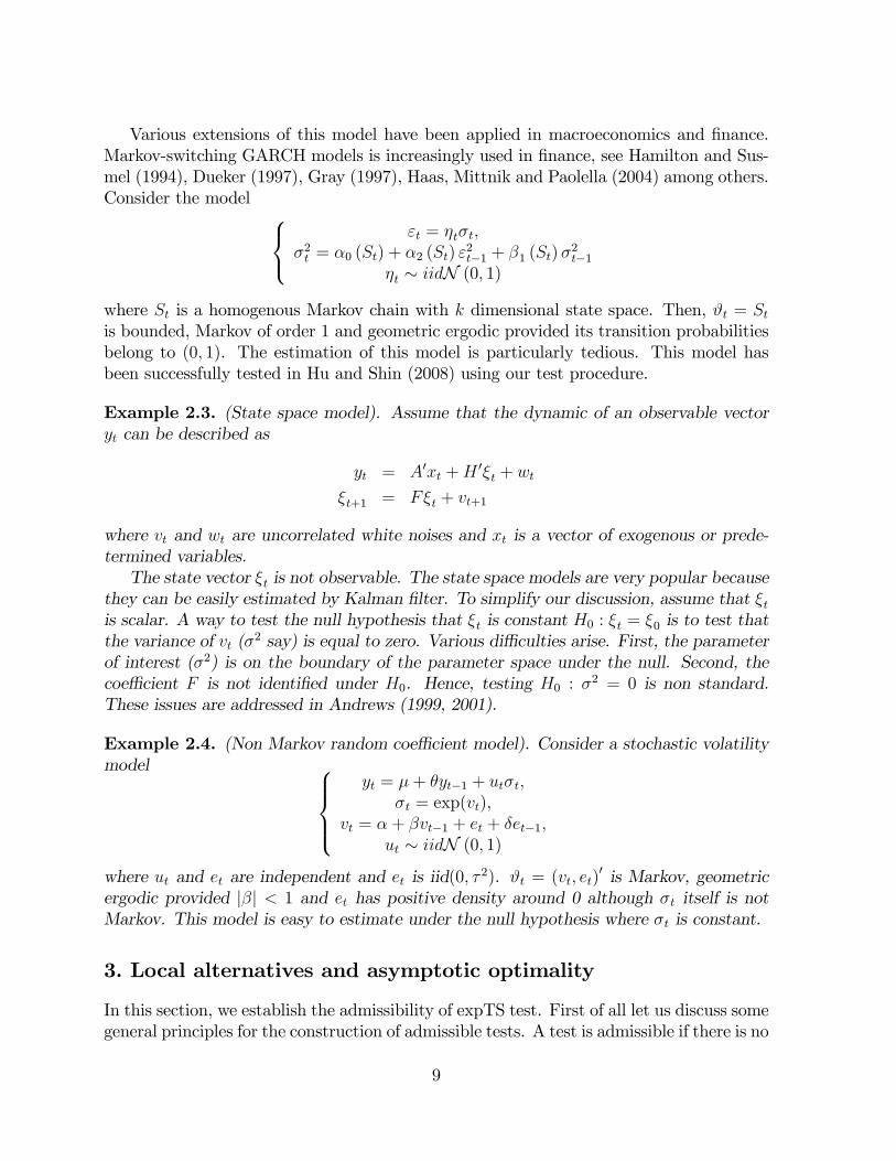
Various extensions of this model have been applied in macroeconomics and �nance.Markov-switching GARCH models is increasingly used in �nance, see Hamilton and Sus-mel (1994), Dueker (1997), Gray (1997), Haas, Mittnik and Paolella (2004) among others.Consider the model 8<:

"t = �t�t;�2t = �0 (St) + �2 (St) "

2t�1 + �1 (St)�

2t�1

�t � iidN (0; 1)

where St is a homogenous Markov chain with k dimensional state space. Then, #t = Stis bounded, Markov of order 1 and geometric ergodic provided its transition probabilitiesbelong to (0; 1). The estimation of this model is particularly tedious. This model hasbeen successfully tested in Hu and Shin (2008) using our test procedure.

Example 2.3. (State space model). Assume that the dynamic of an observable vectoryt can be described as

yt = A0xt +H 0�t + wt

�t+1 = F�t + vt+1

where vt and wt are uncorrelated white noises and xt is a vector of exogenous or prede-termined variables.The state vector �t is not observable. The state space models are very popular because

they can be easily estimated by Kalman �lter. To simplify our discussion, assume that �tis scalar. A way to test the null hypothesis that �t is constant H0 : �t = �0 is to test thatthe variance of vt (�2 say) is equal to zero. Various di¢ culties arise. First, the parameterof interest (�2) is on the boundary of the parameter space under the null. Second, thecoe¢ cient F is not identi�ed under H0. Hence, testing H0 : �

2 = 0 is non standard.These issues are addressed in Andrews (1999, 2001).

Example 2.4. (Non Markov random coe¢ cient model). Consider a stochastic volatilitymodel 8>><>>:

yt = �+ �yt�1 + ut�t;�t = exp(vt);

vt = �+ �vt�1 + et + �et�1;ut � iidN (0; 1)

where ut and et are independent and et is iid(0; � 2). #t = (vt; et)0 is Markov, geometric

ergodic provided j�j < 1 and et has positive density around 0 although �t itself is notMarkov. This model is easy to estimate under the null hypothesis where �t is constant.

3. Local alternatives and asymptotic optimality

In this section, we establish the admissibility of expTS test. First of all let us discuss somegeneral principles for the construction of admissible tests. A test is admissible if there is no

9

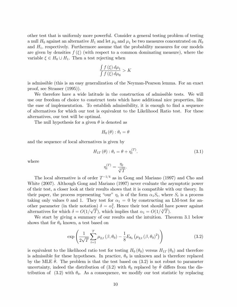
other test that is uniformly more powerful. Consider a general testing problem of testinga null H0 against an alternative H1 and let �0 and �1 be two measures concentrated on H0

and H1; respectively. Furthermore assume that the probability measures for our modelsare given by densities f (�) (with respect to a common dominating measure), where thevariable � 2 H0 [H1. Then a test rejecting whenR

f (�) d�1Rf (�) d�0

> K

is admissible (this is an easy generalization of the Neyman-Pearson lemma. For an exactproof, see Strasser (1995)).We therefore have a wide latitude in the construction of admissible tests. We will

use our freedom of choice to construct tests which have additional nice properties, likethe ease of implementation. To establish admissibility, it is enough to �nd a sequenceof alternatives for which our test is equivalent to the Likelihood Ratio test. For thesealternatives, our test will be optimal.The null hypothesis for a given � is denoted as

H0 (�) : �t = �

and the sequence of local alternatives is given by

H1T (�) : �t = � + �(T )t : (3.1)

where�(T )t =

�t4pT:

The local alternative is of order T�1=4 as in Gong and Mariano (1997) and Cho andWhite (2007). Although Gong and Mariano (1997) never evaluate the asymptotic powerof their test, a closer look at their results shows that it is compatible with our theory. Intheir paper, the process representing �our��t is of the form �1St, where St is a processtaking only values 0 and 1. They test for �1 = 0 by constructing an LM-test for an-other parameter (in their notation) � = �21: Hence their test should have power againstalternatives for which � = O(1=

pT ), which implies that �1 = O(1= 4

pT ):

We start by giving a summary of our results and the intuition. Theorem 3.1 belowshows that for �0 known, a test based on

exp

1

2pT

TXt=1

�2;t (�; �0)�1

8E�0

��2;t (�; �0)

2�! (3.2)

is equivalent to the likelihood ratio test for testing H0 (�0) versus H1T (�0) and thereforeis admissible for these hypotheses. In practice, �0 is unknown and is therefore replacedby the MLE �. The problem is that the test based on (3.2) is not robust to parameteruncertainty, indeed the distribution of (3.2) with �0 replaced by � di¤ers from the dis-tribution of (3.2) with �0. As a consequence, we modify our test statistic by replacing

10

�2;t

��; ��by "t

��; ��, its projection on the space orthogonal to l(1)t

���: The resulting

test statistic is robust to parameter uncertainty. To see this, we apply the mean valuetheorem (� is omitted for convenience):

1pT

TXt=1

"t

���=

1pT

TXt=1

"t (�0) +1

T

TXt=1

@"t���

@�

�� � �0

�where � is an intermediate value. Hence under standard conditions, we have

1

T

TXt=1

@"t���

@�! E�0

�@"t (�0)

@�

�= �cov�0

�"t (�0) ; l

(1)t (�0)

�= 0:

The new test statistic is robust to parameter uncertainty but is no longer equivalent to thelikelihood ratio of H0 (�0) against H1T (�0). We show that it is equivalent to the likelihoodratio of H0 (�0) against

H1T (�T ) : �t = � +�t4pT� dp

T

where d is de�ned in (3.13). Hence, it is optimal for this alternative.Let Q�T denote the joint distribution of (�1; :::; �T ), indexed by the unknown parameter

�. Let P�;� be the probability measure on y1; y2; :::; yT corresponding toH1T (�), and P� bethe probability measure on y1; y2; :::; yT corresponding to H0 (�) : The ratio of the densitiesunder H0 (�) and H1T (�) is given by

`�T (�) �dP�;�dP�

=

Z TYt=1

ft�� + �t=T

1=4�dQ�T=

TYt=1

ft (�) :

Theorem 3.1. Under Assumptions 1-3, we have under H0 (�)

`�T (�) = exp

1

2pT

TXt=1

�2;t (�; �)�1

8E���2;t (�; �)

2�! P! 1: (3.3)

where the convergence in probability is uniform over � and � 2 N .

The proof of Theorem 3.1 is the main contribution of the paper and is given in Ap-pendix B.We can easily see from (2.8) that �2;t (�; �0) is a stationary and ergodic martingale

di¤erence sequence, hence the central limit theorem applies. Moreover, for each sequence

N 3 �T ! �0 2 N ; (3.4)

the distribution of 12pT

PTt=1 �2;t (�; �T ) will converge in distribution, under P�T , to a

Gaussian random variable with expectation 0 and variance 14E��2;t (�; �0)

2� :11

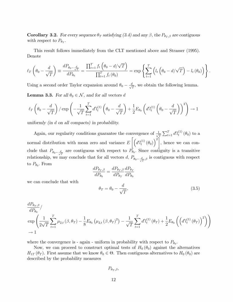
Corollary 3.2. For every sequence �T satisfying (3.4) and any �, the P�T ;� are contiguouswith respect to P�T :

This result follows immediately from the CLT mentioned above and Strasser (1995).Denote

`T

��0 �

dpT

��dP�0� dp

T

dP�0=

QTt=1 ft

��0 � d=

pT�

QTt=1 ft (�0)

= exp

(TXt=1

�lt

��0 � d=

pT�� lt (�0)

�):

Using a second order Taylor expansion around �0 � dpT, we obtain the following lemma.

Lemma 3.3. For all �0 2 N , and for all vectors d

`T

��0 �

dpT

�= exp

� 1p

T

TXt=1

d0l(1)t

��0 �

dpT

�+1

2E�0

�d0l

(1)t

��0 �

dpT

��2!! 1

uniformly (in d on all compacts) in probability.

Again, our regularity conditions guarantee the convergence of 1pT

PTt=1 d

0l(1)t (�0) to a

normal distribution with mean zero and variance E��d0l

(1)t (�0)

�2�, hence we can con-

clude that P�0� dpT

are contiguous with respect to P�0 : Since contiguity is a transitive

relationship, we may conclude that for all vectors d; P�0� dpT;� is contiguous with respect

to P�0 : FromdP�T ;�dP�0

=dP�T ;�dP�T

dP�TdP�0

we can conclude that with

�T = �0 �dpT; (3.5)

dP�T ;�dP�0

=

exp

1

2pT

TXt=1

�2;t (�; �T )�1

8E�0

��2;t (�; �T )

2�� 1pT

TXt=1

d0l(1)t (�T ) +

1

2E�0

��d0l

(1)t (�T )

�2�!! 1

where the convergence is - again - uniform in probability with respect to P�0.Now, we can proceed to construct optimal tests of H0 (�0) against the alternatives

H1T (�T ). First assume that we know �0 2 �. Then contiguous alternatives to H0 (�0) aredescribed by the probability measures

P�T ;�;

12

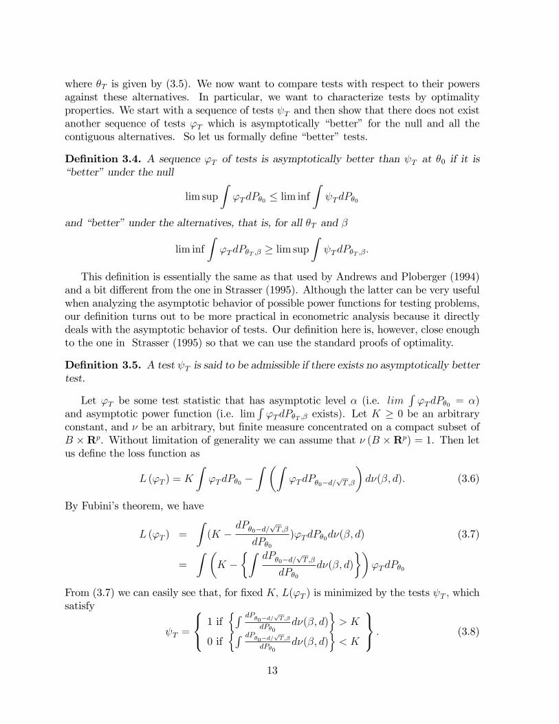
where �T is given by (3.5). We now want to compare tests with respect to their powersagainst these alternatives. In particular, we want to characterize tests by optimalityproperties. We start with a sequence of tests T and then show that there does not existanother sequence of tests 'T which is asymptotically �better� for the null and all thecontiguous alternatives. So let us formally de�ne �better�tests.

De�nition 3.4. A sequence 'T of tests is asymptotically better than T at �0 if it is�better�under the null

lim sup

Z'TdP�0 � lim inf

Z TdP�0

and �better�under the alternatives, that is, for all �T and �

lim inf

Z'TdP�T ;� � lim sup

Z TdP�T ;�:

This de�nition is essentially the same as that used by Andrews and Ploberger (1994)and a bit di¤erent from the one in Strasser (1995). Although the latter can be very usefulwhen analyzing the asymptotic behavior of possible power functions for testing problems,our de�nition turns out to be more practical in econometric analysis because it directlydeals with the asymptotic behavior of tests. Our de�nition here is, however, close enoughto the one in Strasser (1995) so that we can use the standard proofs of optimality.

De�nition 3.5. A test T is said to be admissible if there exists no asymptotically bettertest.

Let 'T be some test statistic that has asymptotic level � (i.e. limR'TdP�0 = �)

and asymptotic power function (i.e. limR'TdP�T ;� exists). Let K � 0 be an arbitrary

constant, and � be an arbitrary, but �nite measure concentrated on a compact subset ofB �Rp. Without limitation of generality we can assume that � (B �Rp) = 1. Then letus de�ne the loss function as

L ('T ) = K

Z'TdP�0 �

Z �Z'TdP�0�d=

pT ;�

�d�(�; d): (3.6)

By Fubini�s theorem, we have

L ('T ) =

Z(K �

dP�0�d=pT ;�

dP�0)'TdP�0d�(�; d) (3.7)

=

Z �K �

�ZdP�0�d=

pT ;�

dP�0d�(�; d)

��'TdP�0

From (3.7) we can easily see that, for �xed K; L('T ) is minimized by the tests T ; whichsatisfy

T =

8<: 1 ifnR dP�0�d=

pT;�

dP�0d�(�; d)

o> K

0 ifnR dP�0�d=

pT;�

dP�0d�(�; d)

o< K

9=; : (3.8)

13

So the minimal loss only depends on the distributions of thenR dP�0�d=

pT;�

dP�0d�(�; d)

o.

We can easily see that the measuresRP�0�d=

pT ;�d�(�; d) are contiguous with respect to

P�0, too. Hence the minimal loss equals

�Z ��Z

dP�0�d=pT ;�

dP�0d�(�; d)

��K

�(+)dP�0;

where, for an arbitrary real number x, x (+) denotes the positive part of x.Let us now assume that we have a competing sequence of tests 'T . Note that

(3.8) does not uniquely determine a test. Indeed, the behavior of the test on the eventhnR dP�0�d=pT;�

dP�0d�(�; d)

o= K

idoes not matter. Hence the following de�nition will be

useful.

De�nition 3.6. The tests 'T and '0T are asymptotically equivalent (with respect to ourloss function L) if and only if for all " > 0

limE�0 j'T � '0T j I������Z dP�0�d=

pT ;�

dP�0d�(�; d)

��K

���� > "

�= 0:

So, heuristically speaking, 'T and '0T give us the same decision provided the test

statisticR dP�0�d=

pT;�

dP�0d�(�; d) is di¤erent from the critical value K. Moreover, we have the

following result.

Theorem 3.7. Let T be de�ned by (3.8) and 'T be an arbitrary test.(i) If 'T and T are asymptotically equivalent in the sense of De�nition 3.6. Then

lim (L( T )� L ('T )) = 0: (3.9)

(ii) If 'T and T are not asymptotically equivalent, then

lim inf (L( T )� L ('T )) < 0: (3.10)

Hence (3.9) implies that T and 'T are asymptotically equivalent.

We conclude from Theorem 3.7 that the tests T and all asymptotically equivalentsequences of tests are admissible. Any tests with genuinely better power functions wouldhave smaller loss, which is impossible. Hence, we have to show that our test is asymptot-ically equivalent to tests T .For this purpose, let us �rst observe that the processes

ZT (�; �) =1

2pT

TXt=1

�2;t (�; �)�1

8E�0

��2;t (�; �)

2�� 1pT

TXt=1

d0l(1)t (�)+

1

2E�0

��d0l

(1)t (�)

�2�;

are, for all � so that k� � �0k = O(1)=pT (and hence in particular the �T de�ned by

(3.5)), uniformly tight in the space C (B), the space of continuous functions on B. Indeed,

14

since the �2;t (�; �T ) are stationary martingale di¤erences, we can apply a central limittheorem and conclude that the ZT (�) converges in distribution (with respect to P�T ) toa Gaussian process with a.s. continuous trajectories. Since the P�T are contiguous to P�0 ;the limiting process(es) under P�0 must have continuous trajectories too, and we haveuniform tightness of the distributions with respect to P�0.

De�nition 3.8. De�ne �T as the tests that reject whenRexp(ZT (�; �T ))d�(�; d) > K

and accept whenRexp(ZT (�; �T ))d�(�; d) < K.

We now want to show that the tests T and �T are asymptotically equivalent. Wecan easily see that a su¢ cient condition for asymptotic equivalence isZ

exp(ZT (�; �T ))d�(�; d)=

ZdP�0�d=

pT ;�

dP�0d�(�; d)! 1: (3.11)

We know that for all �nite sets �i; di;

exp(ZT (�i; �0 � di=pT ))=

dP�0�di=pT ;�i

dP�0! 1: (3.12)

So suppose that for all " > 0 and � > 0; we could �nd a partition S1; :::; SK so that withprobability greater than 1� " for all i, (�; d) ; ( ; e) 2 Si, jZT (�; �0� d=

pT )�ZT ( ; �0�

e=pT )j < �; jdP�0�d=

pT;�

dP�0� dP�0�e=

pT;

dP�0j < �: Then, (3.11) will be an easy consequence of

(3.12).The existence of such a partition for the ZT is an immediate consequence of the

uniform tightness of the distribution of ZT : According to our assumptions, the di¤erence

between the ZT and the log of the densitiesdP�0�di=

pT;�i

dP�0converges to zero uniformly

in probability. Hence the density process is uniformly tight, too, which immediatelyguarantees the existence of the partition.Then, the tests �T are asymptotically equivalent to the tests T . Consequently, we

have the following result.

Theorem 3.9. Let 'T be a sequence of tests that is asymptotically better (in the senseof De�nition 3.4) than �T . Then 'T is asymptotically equivalent to �T .

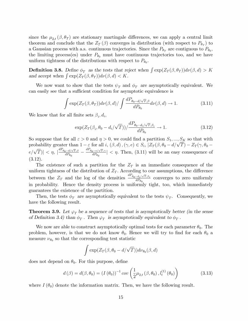
We now are able to construct asymptotically optimal tests for each parameter �0. Theproblem, however, is that we do not know �0: Hence we will try to �nd for each �0 ameasure ��0 so that the corresponding test statisticZ

exp(ZT (�; �0 � d=pT ))d��0(�; d)

does not depend on �0. For this purpose, de�ne

d (�) = d(�; �0) = (I (�0))�1 cov

�1

2�2;t (�; �0) ; l

(1)t (�0)

�(3.13)

where I (�0) denote the information matrix. Then, we have the following result.

15

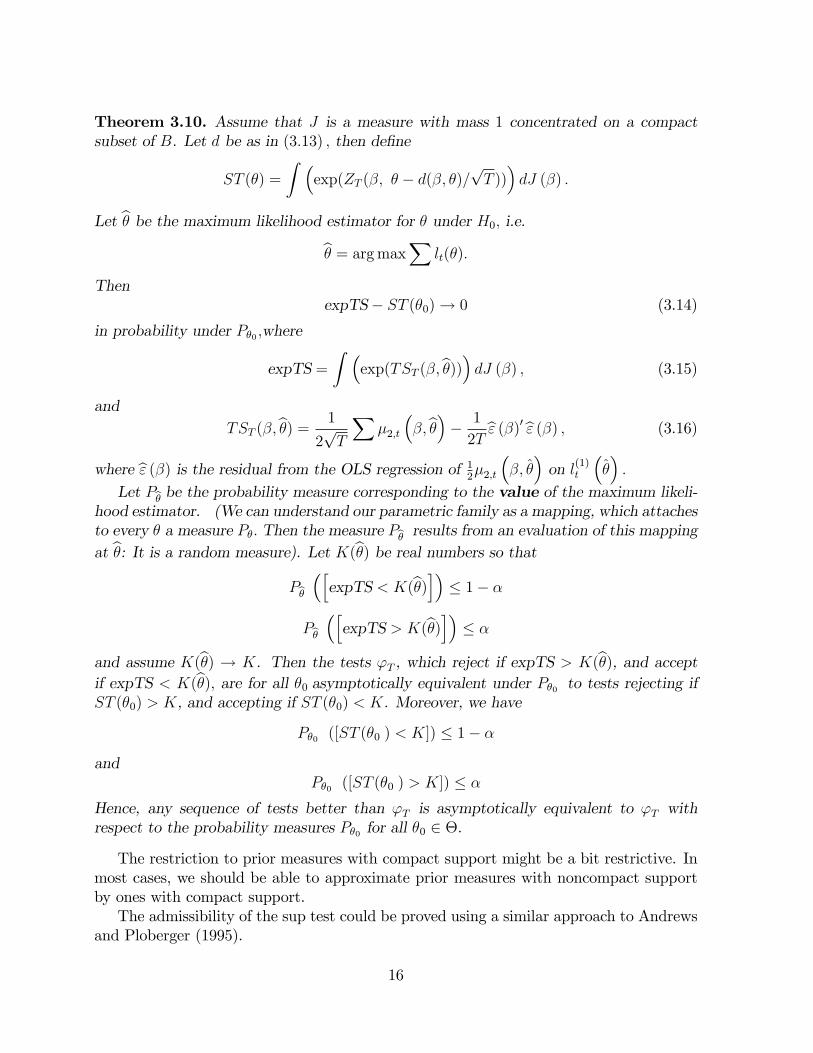
Theorem 3.10. Assume that J is a measure with mass 1 concentrated on a compactsubset of B. Let d be as in (3:13) ; then de�ne

ST (�) =

Z �exp(ZT (�; � � d(�; �)=

pT ))�dJ (�) :

Let b� be the maximum likelihood estimator for � under H0; i.e.b� = argmaxX lt(�):

ThenexpTS� ST (�0)! 0 (3.14)

in probability under P�0 ;where

expTS =Z �

exp(TST (�;b�))� dJ (�) ; (3.15)

andTST (�;b�) = 1

2pT

X�2;t

��;b��� 1

2Tb" (�)0b" (�) ; (3.16)

where b" (�) is the residual from the OLS regression of 12�2;t

��; ��on l(1)t

���:

Let Pb� be the probability measure corresponding to the value of the maximum likeli-hood estimator. (We can understand our parametric family as a mapping, which attachesto every � a measure P�: Then the measure Pb� results from an evaluation of this mappingat b�: It is a random measure). Let K(b�) be real numbers so that

Pb��hexpTS < K(b�)i� � 1� �

Pb��hexpTS > K(b�)i� � �

and assume K(b�) ! K. Then the tests 'T , which reject if expTS > K(b�), and acceptif expTS < K(b�); are for all �0 asymptotically equivalent under P�0 to tests rejecting ifST (�0) > K, and accepting if ST (�0) < K. Moreover, we have

P�0 ([ST (�0 ) < K]) � 1� �

andP�0 ([ST (�0 ) > K]) � �

Hence, any sequence of tests better than 'T is asymptotically equivalent to 'T withrespect to the probability measures P�0 for all �0 2 �.

The restriction to prior measures with compact support might be a bit restrictive. Inmost cases, we should be able to approximate prior measures with noncompact supportby ones with compact support.The admissibility of the sup test could be proved using a similar approach to Andrews

and Ploberger (1995).

16

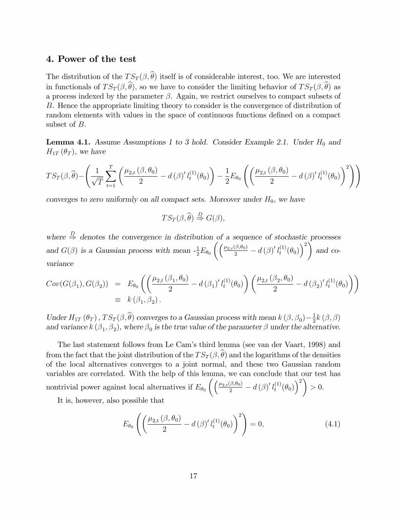
4. Power of the test

The distribution of the TST (�;b�) itself is of considerable interest, too. We are interestedin functionals of TST (�;b�); so we have to consider the limiting behavior of TST (�;b�) asa process indexed by the parameter �. Again, we restrict ourselves to compact subsets ofB. Hence the appropriate limiting theory to consider is the convergence of distribution ofrandom elements with values in the space of continuous functions de�ned on a compactsubset of B.

Lemma 4.1. Assume Assumptions 1 to 3 hold. Consider Example 2.1. Under H0 andH1T (�T ), we have

TST (�;b�)� 1pT

TXt=1

��2;t (�; �0)

2� d (�)0 l

(1)t (�0)

�� 12E�0

��2;t (�; �0)

2� d (�)0 l

(1)t (�0)

�2!!

converges to zero uniformly on all compact sets. Moreover under H0, we have

TST (�;b�) D) G(�);

where D) denotes the convergence in distribution of a sequence of stochastic processes

and G(�) is a Gaussian process with mean -12E�0

���2;t(�;�0)

2� d (�)0 l

(1)t (�0)

�2�and co-

variance

Cov(G(�1); G(�2)) = E�0

���2;t (�1; �0)

2� d (�1)

0 l(1)t (�0)

���2;t (�2; �0)

2� d (�2)

0 l(1)t (�0)

��� k (�1; �2) :

UnderH1T (�T ) ; TST (�;b�) converges to a Gaussian process with mean k (�; �0)� 12k (�; �)

and variance k (�1; �2), where �0 is the true value of the parameter � under the alternative.

The last statement follows from Le Cam�s third lemma (see van der Vaart, 1998) andfrom the fact that the joint distribution of the TST (�;b�) and the logarithms of the densitiesof the local alternatives converges to a joint normal, and these two Gaussian randomvariables are correlated. With the help of this lemma, we can conclude that our test has

nontrivial power against local alternatives if E�0

���2;t(�;�0)

2� d (�)0 l

(1)t (�0)

�2�> 0.

It is, however, also possible that

E�0

��2;t (�; �0)

2� d (�)0 l

(1)t (�0)

�2!= 0; (4.1)

17

in which case TST (�;b�) will converge to zero and the test expTS will have no power.Some insight about this phenomenon can be gained by examining:

E�0

���2;t2� d0l

(1)t

�2�= E�0

���2;t2

�2�� 2d0E�0

�l(1)t

�2;t2

�+ d0 (I (�0))

�1 d

= E�0

���2;t2

�2�� E�0

�l(1)t

�2;t2

�0 �E�0

�l(1)t l

(1)0t

���1E�0

�l(1)t

�2;t2

�using (3.13). Hence (4.1) is satis�ed if and only if �2;t belongs to the linear span of

the components of l(1)t . Another way to see this is the following. Notice that becausePl(1)t

�b�� = 0; P �2;t(�;�)2

=P"t (�) where "t (�) is the projection

�2;t(�;�)2

on the space

orthogonal to l(1)t . Hence, TST (�;b�) can be rewritten asTST (�;b�) = 1p

T

X"t (�)�

1

2T

X"2t (�) :

If �2;t��; ��belongs to the space spanned by l(1)t ; then "t (�) = 0 and TST (�;b�) = 0.

Hence, if �2;t��; ��belongs to the space spanned by l(1)t for all �, the test expTS will have

no power. However, this is unlikely to happen except in very special cases. Let us constructsuch an example. Assume for a moment that � = 0 and all the other prerequisites ofAssumptions 1-3 and Example 2.1 are ful�lled. Then �2;t is a linear functional of the

second-order derivatives of the log-likelihood, namely h0�@2lt@�@�0 +

�@lt@�

� �@lt@�

�0�h. Then

(4.1) means that the second order derivatives can be written as a linear combination ofthe scores. This is a geometric condition, which has profound statistical implications. E.g.in Murray and Rice (1993, p. 16), it is used to characterize linear exponential families. Atypical example would be the normal distribution. We have two parameters, mean andvariance, and we can easily see that if we take h = (1; 0)0 (we allow the mean to switchbut not the variance), then (4.1) is ful�lled (for all � because here � is simply c2). Thiscorresponds to testing for independent mixture of two normals with di¤erent unknownmeans and same unknown variance. This same e¤ect was noticed in Gong and Mariano(1997) who remark that their test does not work in this situation. Note that on theother hand, our test has power against a Markov-switching model (� 6= 0) with unknownswitching mean and unknown constant variance. This case will be examined in details inSection 5.If (4.1) is ful�lled for all �, then it is impossible to construct a test with nontrivial power

against these speci�c local alternatives. The TST (�;b�) are consistent approximations ofthe log-density of one measure under the null (corresponding to �0 and to �0 � d=

pT ,

�, respectively). If the density between these two measures converges to 1, then anyreasonable distance like e.g. total variation converges to zero. So in this kind of situation

18

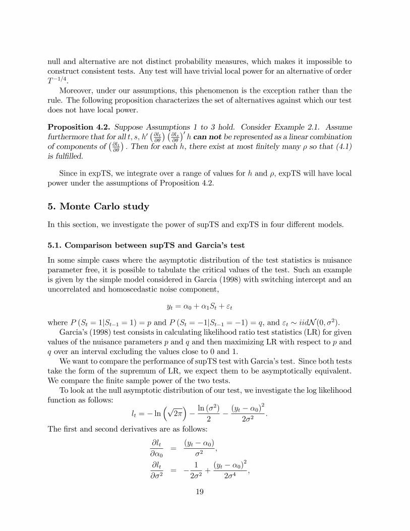
null and alternative are not distinct probability measures, which makes it impossible toconstruct consistent tests. Any test will have trivial local power for an alternative of orderT�1=4.Moreover, under our assumptions, this phenomenon is the exception rather than the

rule. The following proposition characterizes the set of alternatives against which our testdoes not have local power.

Proposition 4.2. Suppose Assumptions 1 to 3 hold. Consider Example 2.1. Assumefurthermore that for all t; s; h0

�@lt@�

� �@ls@�

�0h can not be represented as a linear combination

of components of�@lt@�

�: Then for each h, there exist at most �nitely many � so that (4.1)

is ful�lled.

Since in expTS, we integrate over a range of values for h and �; expTS will have localpower under the assumptions of Proposition 4.2.

5. Monte Carlo study

In this section, we investigate the power of supTS and expTS in four di¤erent models.

5.1. Comparison between supTS and Garcia�s test

In some simple cases where the asymptotic distribution of the test statistics is nuisanceparameter free, it is possible to tabulate the critical values of the test. Such an exampleis given by the simple model considered in Garcia (1998) with switching intercept and anuncorrelated and homoscedastic noise component,

yt = �0 + �1St + "t

where P (St = 1jSt�1 = 1) = p and P (St = �1jSt�1 = �1) = q, and "t � iidN (0; �2):Garcia�s (1998) test consists in calculating likelihood ratio test statistics (LR) for given

values of the nuisance parameters p and q and then maximizing LR with respect to p andq over an interval excluding the values close to 0 and 1.We want to compare the performance of supTS test with Garcia�s test. Since both tests

take the form of the supremum of LR, we expect them to be asymptotically equivalent.We compare the �nite sample power of the two tests.To look at the null asymptotic distribution of our test, we investigate the log likelihood

function as follows:

lt = � ln�p2��� ln (�

2)

2� (yt � �0)

2

2�2:

The �rst and second derivatives are as follows:

@lt@�0

=(yt � �0)

�2;

@lt@�2

= � 1

2�2+(yt � �0)

2

2�4;

19

@2lt@�20

= � 1

�2;

@2lt

@ (�2)2=

1

2�4� (yt � �0)

2

�6;

@2lt@�0@�2

= �(yt � �0)

�4:

So we have

l(1)t

���=

ut�2

u2t��22�4

!where ut = yt � �0 = yt � �Y .Notice that the variance �2 is unknown yet �xed, which implies that �t =

��1St 0

�0following our notation. Then we have E(�t�

0s) = c2

��t�s 00 0

�: As a consequence,

trace��l(2)t + l

(1)t l

(1)0t

�E (�t�

0t)�is equal to the (1; 1) element of

�l(2)t + l

(1)t l

(1)0t

�times c2,

namely,

trace��l(2)t + l

(1)t l

(1)0t

�E (�t�

0t)�= c2

�u2t � �2

��4

:

Similarly, we have

trace��l(1)t l(1)0s

�E (�t�

0s)�= c2�t�s

utus

�4:

Hence,1

2c2�2;t(�) =

1

2�4

"�u2t � �2

�+ 2

Xs<t

�(t�s)utus

#and

��T (�) =1

2pT �4

X"�u2t � �2

�+ 2

Xs<t

�(t�s)utus

#(5.1)

Moreover, recall that the MLE of �2 is simply

�2 =

P�yt � �Y

�2T

=

Pu2tT

:

It follows that

1pT

Xt

�u2t � �2

�=pT1

T

Xt

�u2t � �2

�=pT��2 � �2

�= 0:

Hence, ��T (�) simpli�es:

��T (�) =1pT �4

Xt

Xs<t

�(t�s)utus: (5.2)

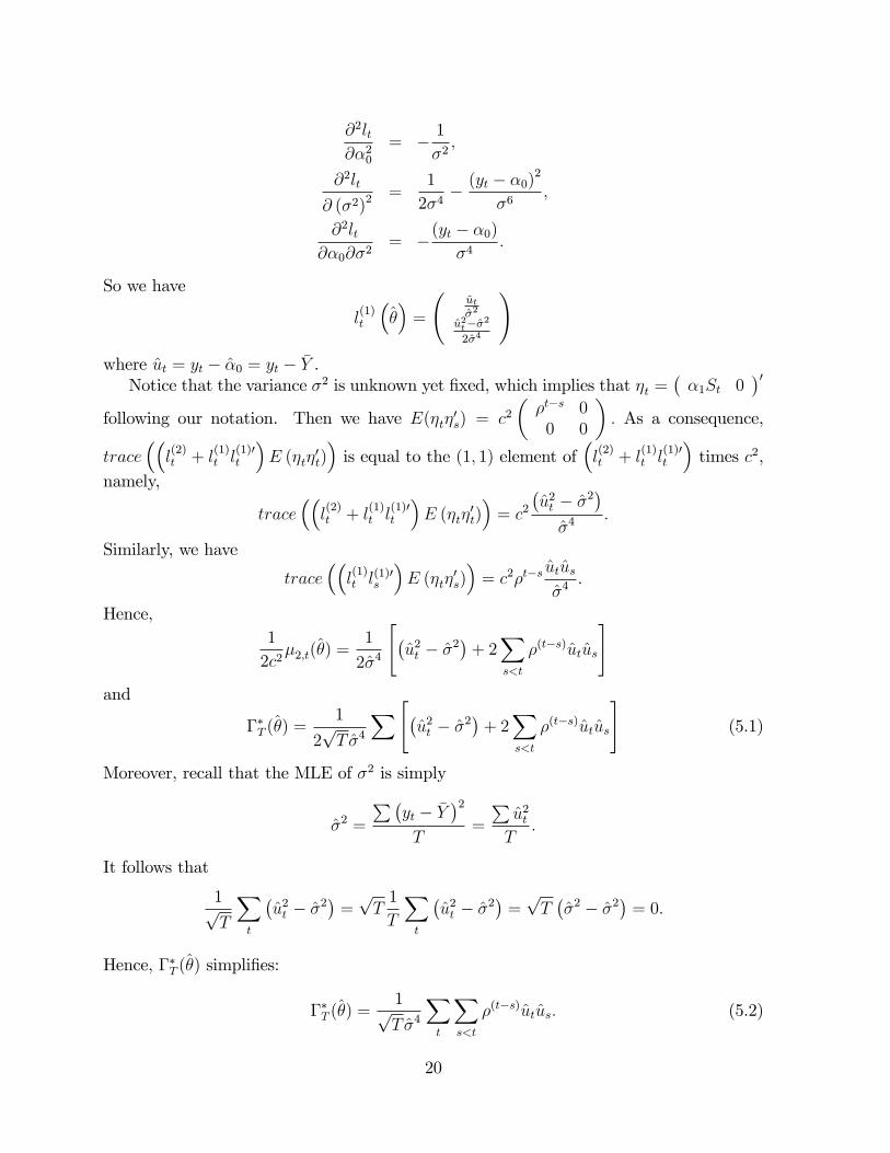
20

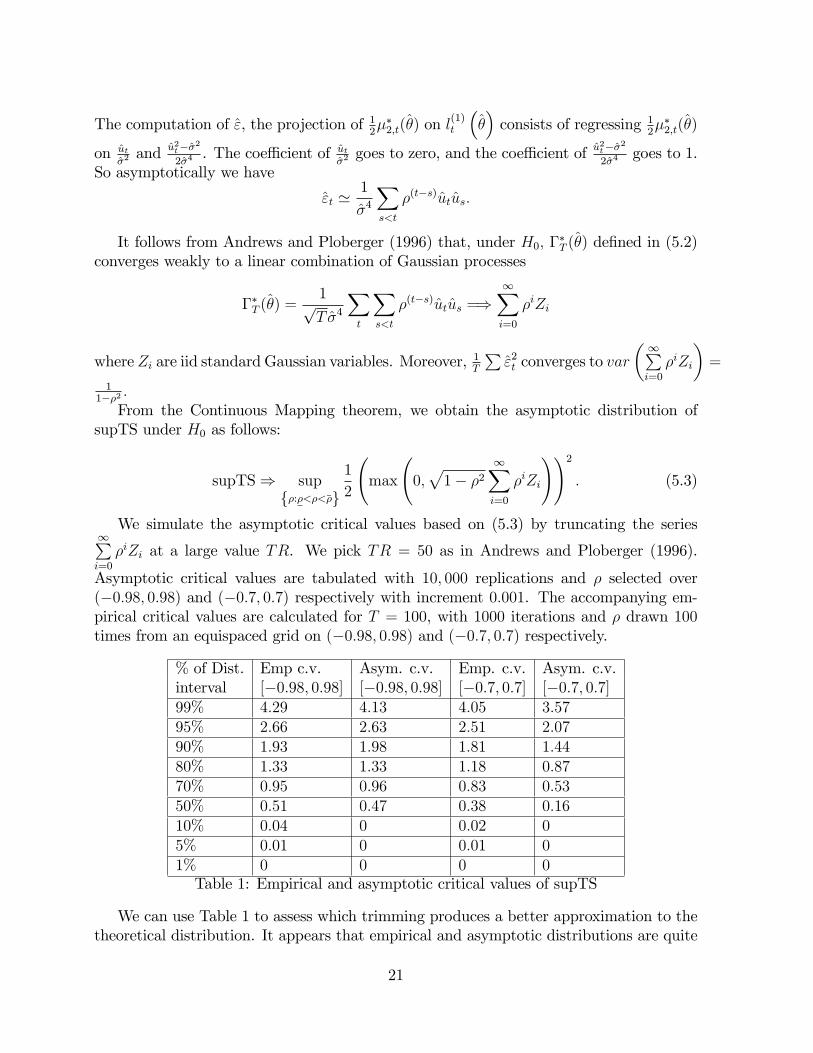
The computation of ", the projection of 12��2;t(�) on l

(1)t

���consists of regressing 1

2��2;t(�)

on ut�2and u2t��2

2�4. The coe¢ cient of ut

�2goes to zero, and the coe¢ cient of u

2t��22�4

goes to 1.So asymptotically we have

"t '1

�4

Xs<t

�(t�s)utus:

It follows from Andrews and Ploberger (1996) that, under H0; ��T (�) de�ned in (5.2)

converges weakly to a linear combination of Gaussian processes

��T (�) =1pT �4

Xt

Xs<t

�(t�s)utus =)1Xi=0

�iZi

where Zi are iid standard Gaussian variables. Moreover, 1TP"2t converges to var

� 1Pi=0

�iZi

�=

11��2 :From the Continuous Mapping theorem, we obtain the asymptotic distribution of

supTS under H0 as follows:

supTS) supf�:�<�<��g

1

2

max

0;p1� �2

1Xi=0

�iZi

!!2: (5.3)

We simulate the asymptotic critical values based on (5.3) by truncating the series1Pi=0

�iZi at a large value TR. We pick TR = 50 as in Andrews and Ploberger (1996).

Asymptotic critical values are tabulated with 10; 000 replications and � selected over(�0:98; 0:98) and (�0:7; 0:7) respectively with increment 0:001. The accompanying em-pirical critical values are calculated for T = 100, with 1000 iterations and � drawn 100times from an equispaced grid on (�0:98; 0:98) and (�0:7; 0:7) respectively.

% of Dist. Emp c.v. Asym. c.v. Emp. c.v. Asym. c.v.interval [�0:98; 0:98] [�0:98; 0:98] [�0:7; 0:7] [�0:7; 0:7]99% 4:29 4:13 4:05 3:5795% 2:66 2:63 2:51 2:0790% 1:93 1:98 1:81 1:4480% 1:33 1:33 1:18 0:8770% 0:95 0:96 0:83 0:5350% 0:51 0:47 0:38 0:1610% 0:04 0 0:02 05% 0:01 0 0:01 01% 0 0 0 0Table 1: Empirical and asymptotic critical values of supTS

We can use Table 1 to assess which trimming produces a better approximation to thetheoretical distribution. It appears that empirical and asymptotic distributions are quite

21

close in the case of [�0:98; 0:98] interval. Note that the asymptotic critical values aremuch lower than those provided by Garcia and are also smaller than the cut-o¤ pointsgiven by a �2(1), the distribution obtained in the standard case.Now we can compare the power performance of supTS with Garcia�s test. The power

of our test is based on the asymptotic critical values tabulated in Table 1 with interval[�0:98; 0:98]. We draw � 100 times from an equispaced grid. Asymptotic critical valuesfor the interval [0:01; 0:99] from Table 1A in Garcia (1998) are used for his test. This isa fair comparison since � 2 [0:01; 0:99] corresponds to � 2 [�0:98; 0:98] in our case1. Wegenerate the data with p = q = 0:75, �0 = 0 and �1 = c= 4

pT : The sample size is 100 and

the number of iterations is 1000.The problem of local maxima may arise in Garcia�s test (see Hamilton (1989) and Gar-

cia (1998)). We follow the standard method and estimate the model using EM algorithmwith 12 sets of starting values and take the maximum over the values so obtained.We plot the power as a function of c in Figure B.1. The case c = 0 corresponds to the

size of the tests. Garcia�s test seems to su¤er from bigger size distortions than ours. Bothtests perform quite well, yet supTS is more powerful than Garcia�s in general. Only whenthe alternative is far away from the null (c = 4 here), his test performs slightly better.

5.2. Power of supTS and expTS in three di¤erent models

We now investigate the power of supTS and expTS in three di¤erent models. In general,the asymptotic distribution of our tests will not be nuisance parameter free. We rely onparametric bootstrap to compute the critical values.For supTS, we search the maximum over h and � in (2.11) by generating h uniformly

over the unit sphere and selecting � from an equispaced grid over (�0:7; 0:7) 2: The numberof values for h is 30 and for � is 403. We obtain the empirical critical values with 1000iterations and sample size equal to 200. Then, we compute the size-corrected power withthe same number of iterations and same sample sizes.The evaluation of the expTS statistic is more involved since we need to pick some

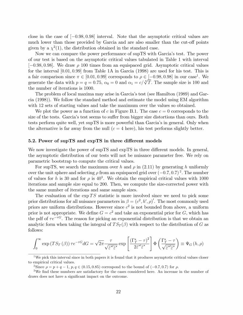
prior distributions for all nuisance parameters in � = (c2; h0; �)0. The most commonly usedpriors are uniform distributions. However since c2 is not bounded from above, a uniformprior is not appropriate. We de�ne G = c2 and take an exponential prior for G, which hasthe pdf of �e��G. The reason for picking an exponential distribution is that we obtain ananalytic form when taking the integral of TST (�) with respect to the distribution of G asfollows:Z 1

0

exp (TST (�)) �e��GdG =

p2�

�p"�0"�

exp

"(��T � �)2

2"�0"�

#�

���T � �p"�0"�

�� G (h; �)

1We pick this interval since in both papers it is found that it produces asymptotic critical values closerto empirical critical values.

2Since � = p+ q � 1; p; q 2 (0:15; 0:85) correspond to the bound of (�0:7; 0:7) for �:3We �nd these numbers are satisfactory for the cases considered here. An increase in the number of

draws does not have a signi�cant impact on the outcome.

22

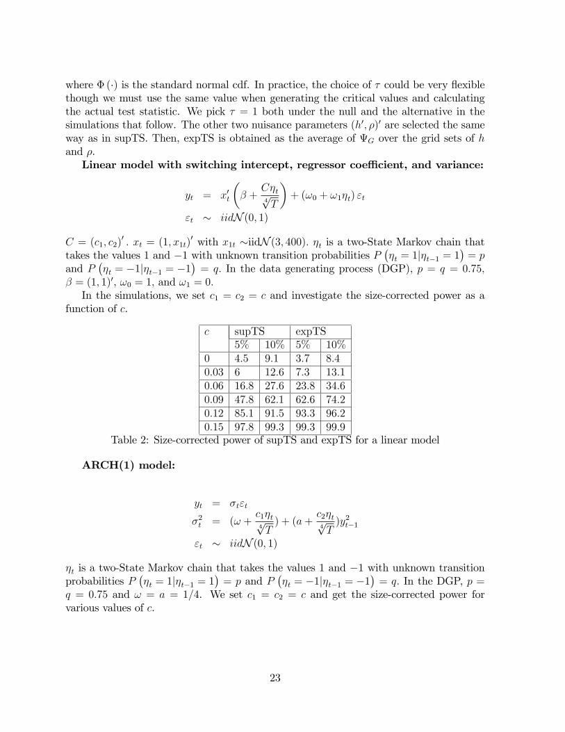
where � (�) is the standard normal cdf. In practice, the choice of � could be very �exiblethough we must use the same value when generating the critical values and calculatingthe actual test statistic. We pick � = 1 both under the null and the alternative in thesimulations that follow. The other two nuisance parameters (h0; �)0 are selected the sameway as in supTS. Then, expTS is obtained as the average of G over the grid sets of hand �.Linear model with switching intercept, regressor coe¢ cient, and variance:

yt = x0t

�� +

C�t4pT

�+ (!0 + !1�t) "t

"t � iidN (0; 1)

C = (c1; c2)0 : xt = (1; x1t)

0 with x1t �iidN (3; 400): �t is a two-State Markov chain thattakes the values 1 and �1 with unknown transition probabilities P

��t = 1j�t�1 = 1

�= p

and P��t = �1j�t�1 = �1

�= q: In the data generating process (DGP), p = q = 0:75;

� = (1; 1)0, !0 = 1; and !1 = 0:In the simulations, we set c1 = c2 = c and investigate the size-corrected power as a

function of c.

c supTS expTS5% 10% 5% 10%

0 4:5 9:1 3:7 8:40:03 6 12:6 7:3 13:10:06 16:8 27:6 23:8 34:60:09 47:8 62:1 62:6 74:20:12 85:1 91:5 93:3 96:20:15 97:8 99:3 99:3 99:9

Table 2: Size-corrected power of supTS and expTS for a linear model

ARCH(1) model:

yt = �t"t

�2t = (! +c1�t4pT) + (a+

c2�t4pT)y2t�1

"t � iidN (0; 1)

�t is a two-State Markov chain that takes the values 1 and �1 with unknown transitionprobabilities P

��t = 1j�t�1 = 1

�= p and P

��t = �1j�t�1 = �1

�= q: In the DGP, p =

q = 0:75 and ! = a = 1=4. We set c1 = c2 = c and get the size-corrected power forvarious values of c.

23

c supTS expTS5% 10% 5% 10%

0 3:9 9:9 5:7 11:30:15 5:9 12:6 5:9 11:40:30 13:5 27:8 18:9 29:10:45 31:7 50 42 54:70:60 68:8 83:1 80 87:40:75 96:8 99:2 98:6 99:1

Table 3: Size-corrected power of supTS and expTS for an ARCH model

IGARCH(1,1):The model is as follows:

yt = �t"t

�2t = (! +c1�t4pT) + (a+

c2�t4pT)�2t�1 + (b+

c3�t4pT)y2t�1

"t � iidN (0; 1)

Here, we let �t take the values 0 and �1 with unknown transition probabilities P (�t =0j�t�1 = 0) = p and P (�t = �1j�t�1 = �1) = q: In the DGP p = q = 0:75 and! = a = b = 1=2: Note that under H0; the model is a IGARCH. c1; c2; and c3 are takento be equal to c. The size-corrected power is given below.

c supTS expTS5% 10% 5% 10%

0 4:9 10:3 4:2 11:10:3 7 14:8 6:6 12:30:6 11:8 20:7 11:4 21:70:9 29:5 42:3 27:4 381:2 49:6 64:6 51:1 61:81:5 87:4 93:9 86:5 90:3

Table 4: Size-corrected power of supTS and expTS for a GARCH model

Remarks.1. Our tests perform very satisfactorily in all cases. As the alternative is more distant

from the null, the power increases monotonically and goes very fast to 100.2. In linear and ARCH cases, expTS performs slightly better than supTS: The pattern

is less clear in IGARCH case.3. Since both supTS and expTS perform very well, we use supTS in the empirical

application because selecting the prior distribution is somewhat arbitrary.

6. Asymmetry in stock price dynamics

As noted by Neftçi (1984) and Hamilton (2004), the major macroeconomic variablesdisplay an asymmetric behavior over various phases of the business cycle. In this section,

24

we are interested in the stock price dynamics. Let Pt and Dt be the stock price indexand dividend at time t: First we estimate the following cointegration relationship betweenln (Pt) and ln (Dt)

ln (Pt) = a0 + a1 ln (Dt) + yt (6.1)

by ordinary least-squares. As Dt plays the role of fundamentals (in the spirit of Lucas,1978, Blanchard and Watson, 1982, and Froot and Obstfeld, 1991), we expect the residualyt to exhibit periods of slow increases (expansions) and sharp declines (recessions). Tocorroborate this intuition, we will �rst test for nonlinearity and then �t the data with aMarkov-switching model.DataWe use monthly US data from 1871-01 to 2004-06 (T =1602) for real S&P composite

stock price index and real dividends. All prices are in January 2000 dollars. These dataare taken from Robert Shiller�s web site http://www.econ.yale.edu/~shiller and describedin Shiller (2000).TestsApplying a BIC criterion on an autoregressive model for yt reveals that 2 lags are best.

The augmented Dickey Fuller test (based on an AR(2)) rejects the null of a unit root onyt at a 1% level. This permits to conclude that yt is stationary. However, we know fromYao and Attali (2000) that markov-switching process may be stationary even if there isan explosive root in one of the regimes. Therefore testing the stationarity of fytg alonedoes not preclude the possibility of lapses of explosive behaviors or booms.Now we wish to test whether yt is better described by an AR(2) process with constant

parameters or with switching coe¢ cients and switching variance. We apply the supTStest (described in (2.10) and (2.11)) where the maximum over h and � is obtained bydrawing h uniformly over the unit sphere (30 values used) and by taking the values of� in an equally spaced grid over (�0:7; 0:7) (60 values used). Empirical critical valuesare computed from 1000 iterations for a sample size equal to the size of the original dataset. The values of the parameters used to simulate the series are those obtained whenestimating the model under H0. The critical values are 5.658, 4.248, 3.768 at 1%, 5% and10% respectively. The test statistic for our data is 22.938. Hence our linearity test rejectsstrongly the null of a linear model versus a Markov-switching alternative, suggesting thatat least two regimes should be used to �t the data.EstimationNow we �t on yt a three-regime Markov-switching model where both the mean and

variance are allowed to switch. As pointed out by Clements and Krolzig (2003), thethree-regime model can capture business cycle asymmetries that are not captured by atwo-regime model.

�yt =Xst

�st +Xst

�styt�1 +lXi=1

�i�yt�i + �st"t (6.2)

where "t � iidN (0; 1). St is an exogenous three-state Markov chain that takes thevalues 1, 2, and 3 and has for transition probabilities 0 < pij < 1. Because the labels

25

of the regimes are interchangeable, we set �1 � �2 � �3: The parameter of interest is� = (�1; �2; �3; �1; �2; �3; �i : i = 1; ::; l; �

21; �

22; �

23; pij : i; j = 1; 2; 3)

0: The coe¢ cients �i

are set constant across regimes because preliminary estimations showed that they did notchange values. The following proposition justi�es our two-step approach.

Proposition 6.1. Assume ln (Dt) is strictly exogenous for "t, in the sense that "t isuncorrelated with ln (D1) ; ln (D2) ; ::; ln (DT ). The MLE estimates of (a0; a1; �) coincidewith the estimators obtained from a two-step procedure consisting in estimating (a0; a1)

0

by OLS in (6.1) �rst and then applying MLE on (6.2). Moreover the resulting � areindependent of (a0; a1) implying that the �rst step does not a¤ect the second step.

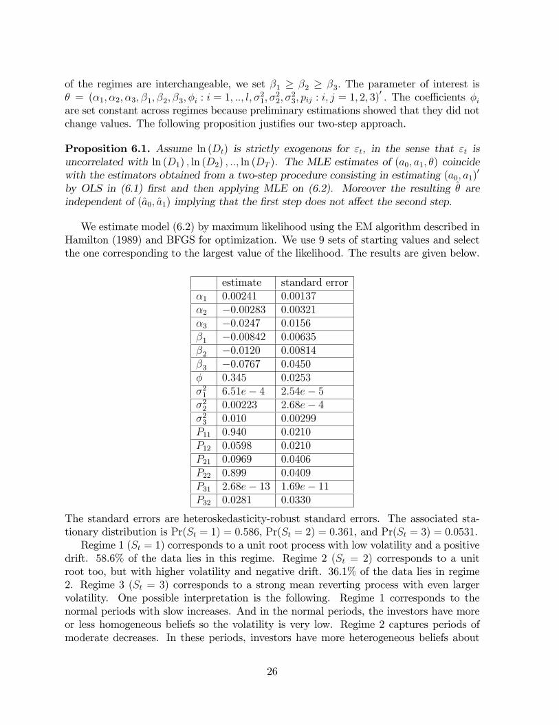
We estimate model (6.2) by maximum likelihood using the EM algorithm described inHamilton (1989) and BFGS for optimization. We use 9 sets of starting values and selectthe one corresponding to the largest value of the likelihood. The results are given below.

estimate standard error�1 0:00241 0:00137�2 �0:00283 0:00321�3 �0:0247 0:0156�1 �0:00842 0:00635�2 �0:0120 0:00814�3 �0:0767 0:0450� 0:345 0:0253�21 6:51e� 4 2:54e� 5�22 0:00223 2:68e� 4�23 0:010 0:00299P11 0:940 0:0210P12 0:0598 0:0210P21 0:0969 0:0406P22 0:899 0:0409P31 2:68e� 13 1:69e� 11P32 0:0281 0:0330

The standard errors are heteroskedasticity-robust standard errors. The associated sta-tionary distribution is Pr(St = 1) = 0:586, Pr(St = 2) = 0:361, and Pr(St = 3) = 0:0531:Regime 1 (St = 1) corresponds to a unit root process with low volatility and a positive

drift. 58.6% of the data lies in this regime. Regime 2 (St = 2) corresponds to a unitroot too, but with higher volatility and negative drift. 36.1% of the data lies in regime2. Regime 3 (St = 3) corresponds to a strong mean reverting process with even largervolatility. One possible interpretation is the following. Regime 1 corresponds to thenormal periods with slow increases. And in the normal periods, the investors have moreor less homogeneous beliefs so the volatility is very low. Regime 2 captures periods ofmoderate decreases. In these periods, investors have more heterogeneous beliefs about

26

the market behavior, which leads to a larger volatility compared to Regime 1. Regime3 represents the crisis regime. It corresponds to sharp declines accompanied by a largevolatility.Through �ltering, we compute the probabilities to be in regime i conditional on the

data: Pr(St = ijy1; :::; yT ): When the probability is greater than 0.5, it is considered thatthe process at time t is in regime i. Regime 3 corresponds to the following two periods:October 1929 to November 1933 and April 1937 to November 1939. Regime 3 identi�es thebig crash in October 1929 and another sharp decline in the stock market price experiencedin 1937. Similarly we isolate the dates where Regime 2 dominates. Starting in 1950, thesedates are 1950 (6-12), 1951 (1-3), 1955 (6-12), 1956 (1-9), 1957 (8-10), 1962 (3-11), 1966(3-9), 1969 (12), 1970 (1-8), 1971 (11-12), October 1973 to January 1976, 1980 (1-5),1981 (7-12), 1982 (1-10), 1984 (8), 1987 (7-12), 1988 (1,2), 1990 (7-12), 1991 (1-3), 1997(4-6), 1998 (6-12), 1999 (1-11), and January 2001 to May 2003. Regime 2 correspondsroughly to the bear market and captures most of the droughts in the US stock marketcycles reported by Pagan and Sossounov (2003) including the crash of October 1987 andthe information technology crisis of 2001-2002.In Figure B.2, we plot the graphs of the probabilities of the three regimes. In the

background of each plot, there is the graph of the log stock price centered by its mean overthe full data set and rescaled so that the maximum value equals 1. The process yt spendsmost of the time in the unit-root regime 1. It follows an asymmetric pattern exhibitingslow increases and fast decreases that are well captured by the Markov-switching model.

7. Conclusion

This paper presents the �rst optimal test against Markov switching alternatives. Ourtest applies to a wide range of models that are popular in macroeconomics and �nance.It is simple to implement as it requires only the estimation of the parameters under thenull hypothesis of constant parameters. Hence, it should be used as a �rst step beforeestimating a complicated nonlinear model.Our test relies on a prior distribution for the switching coe¢ cients �t and, in this

sense, has a Bayesian interpretation. Bayesian inference for Markov-switching models isan active research area, see e.g. Chib (1996), Kim and Nelson (1999), Frühwirth-Schnatter(2001).

27

References

[1] Andrews, D.W.K, (1993). �Tests for Parameter Instability and Structural ChangePoint�, Econometrica, 61, 821-856.

[2] Andrews, D. (1994) �Empirical process methods in econometrics�, in Handbook ofEconometrics, Vol. IV, ed. by R.F. Engle and D.L. McFadden.

[3] Andrews, D. (1999) �Estimation When a Parameter Is on the Boundary�, Econo-metrica, 67, 1341-1383.

[4] Andrews, D. (2001) �Testing When a Parameter Is on the Boundary of the Main-tained Hypothesis�, Econometrica, 69, 683-734.

[5] Andrews, D.W.K., Ploberger, W., (1994). �Optimal Tests When a Nuisance Para-meter Is Present Only under the Alternative�, Econometrica, 62, 1383-1414.

[6] Andrews, D.W.K., Ploberger, W. (1995). �Admissibility of the likelihood ratio testwhen a nuisance parameter is present only under the alternative�, The Annals ofStatistics 23, 1609-1629.

[7] Andrews, D. and W. Ploberger (1996) �Testing for Serial Correlation Against anARMA(1,1) Process�, Journal of the American Statistical Association, Vol. 91, 1331-1342.

[8] Bartle, R. G. (1966) The elements of integration, Wiley and Sons, NY.

[9] Bartlett, M. S. (1953a) �Approximate con�dence intervals�, Biometrika, 40, 12-19.

[10] Bartlett, M. S. (1953b) �Approximate con�dence intervals, II. More than one para-meter�, Biometrika, 40, 306-317.

[11] Blanchard, O. and M.Watson (1982) �Bubbles, Rational Expectations, and FinancialMarkets�, in Crises in the Economic and Financial Structure, ed. by P. Wachtel,LexingtonBooks, Lexington, MA.

[12] Chesher, A. (1984) �Testing for Neglected Heterogeneity�, Econometrica, 52, 865-872.

[13] Chib, S. (1996) �Calculating posterior distributions and modal estimates in Markovmixture models�, Journal of Econometrics, 75, 79-97.

[14] Chirinko, R. and H. Schaller (2001) �Business Fixed Investment and �Bubbles�: TheJapanese Case�, American Economic Review, 91, 663-680.

[15] Cho, J.S. and H. White (2007) �Testing for Regime Switching�, Econometrica, 75,1671-1720.

28

[16] Clements, M. and H.-M. Krolzig (2003) �Business Cycle Asymmetries: Characteriza-tion and Testing Based on Markov-Switching Autoregressions�, Journal of Businessand Economic Statistics, 21, 196-211.

[17] Cox D.R. and H. D. Miller (1965) The Theory of Stochastic Processes, Methuen &Co. Ltd, London, UK.

[18] Davidson, R. and J. MacKinnon (1991) �Une nouvelle forme du test de la matriced�information�, Annales d�Economie et de Statistique, N. 20/21, 171-192.

[19] Davidson, R. and J. MacKinnon (2004) Econometric Theory and Methods, OxfordUniversity Press, New York.

[20] Davies, R.B. (1977) �Hypothesis testing when a nuisance parameter is present onlyunder the alternative�Biometrika, 64, 247-254.

[21] Davies, R.B. (1987) �Hypothesis testing when a nuisance parameter is present onlyunder the alternative�Biometrika, 74, 1, 33-43.

[22] Doukhan, P. (1994) Mixing: Properties and Example, Springer-Verlag, New York.

[23] Dueker, M.J. (1997) �Markov Switching in GARCH Processes and Mean-RevertingStock Market Volatility�, Journal of Business & Economic Statistics, 15/1, 26-34.

[24] Froot, K. and M. Obstfeld (1991) �Intrinsic Bubbles: The Case of Stock Prices�,American Economic Review, 81, 1189-1213.

[25] Frühwirth-Schnatter, S. (2001) �Markov Chain Monte Carlo Estimation of Classicaland Dynamic Switching and Mixture Models�, Journal of the American StatisticalAssociation, 96, 194-209.

[26] Garcia, R.(1998). �Asymptotic Null Distribution of the Likelihood Ratio Test inMarkov Switching Models�, International Economic Review, 39, 763-788.

[27] Gong, F. and Mariano, R.S. (1997). �Testing Under Non-Standard Conditions inFrequency Domain: With Applications to Markov Regime Switching Models of Ex-change Rates and the Federal Funds Rate�, Federal Reserve Bank of New York Sta¤Reports, No. 23.

[28] Gray, S. (1996), �Modeling the Conditional Distribution of Interest Rates as aRegime-Switching Process,�Journal of Financial Economics, 42, 27-62.

[29] Haas, M., S. Mittnik, and M. Paolella (2004), �A New Approach to Markov-SwitchingGARCH Models,�Journal of Financial Econometrics, 2, 493-530.

[30] Hamilton, J.D. 1989. �A new Approach to the Economic Analysis of NonstationaryTime Series and the Business Cycle�, Econometrica 57, 357-384.

29

[31] Hamilton, J. D., and R. Susmel (1994), �Autoregressive Conditional Heteroskedas-ticity and Changes in Regime�, Journal of Econometrics 64, 307-333.

[32] Hamilton, J.D. (2005) �What�s Real About the Business Cycle?�, Federal ReserveBank of St Louis Review, 87, 435-452.

[33] Hansen, B. (1992) �The Likelihood Ratio Test Under Non-Standard Conditions:Testing the Markov Switching Model of GNP�, Journal of Applied Econometrics,7, S61-S82.

[34] Hu, L. (2008) �Optimal Test for Stochastic Unit Root with Markov Switching�,mimeo, Leeds University.

[35] Hu, L. and Y. Shin (2008) �Optimal Testing for Markov Switching GARCHModels�,Studies in Nonlinear Dynamics and Econometrics, 12, Issue 3.

[36] Kahn, J. and R. Rich (2007) �Tracking the New Economy: Using Growth Theory toDetect Changes in Trend Productivity�, forthcoming in Journal of Monetary Eco-nomics.

[37] Kim, C.-J. and C. Nelson (1999) State-Space Models with Regime Switching, MITPress.

[38] Kim, C.-J. and C. Nelson (2001) �A Bayesian Approach to Testing for Markov Switch-ing in Univariate and Dynamic Factor Models�, International Economic Review, 42,989-1013.

[39] Lang, S. (1993) Real and Functional Analysis, Springer-Verlag, New York.

[40] Lee, L-F. and A. Chesher (1984) �Speci�cation Testing when Score Test StatisticsAre Identically Zero�, Journal of Econometrics, 31, 121-149.

[41] Lucas, R. (1978) �Asset Prices in an Exchange Economy�, Econometrica, 66, 429-445.

[42] Morley, J. and J. Piger (2006) �The importance of Nonlinearity in ReproducingBusiness Cycle Features�, in Nonlinear Time Series Analysis of Business Cycles,edited by C. Milas, P. Rothman, and D. van Dijk. Elsevier, Amsterdam.

[43] Murray, M.K and J.W. Rice (1993) Di¤erential Geometry and Statistics, Chapman-Hall, London.

[44] Neftçi, S. (1984) �Are Economic Time Series Asymmetric over the Business Cycle?�,Journal of Political Economy, 92, 307-328.

[45] Pagan, A. and K. Sossounov (2003) �A simple framework for analysing bull and bearmarkets�, Journal of Applied Econometrics, 18, 23-46.

30

[46] Rotnitzky, A., D. Cox, M. Bottai, and J. Robins (2000) �Likelihood-based inferencewith singular information matrix�, Bernoulli, 62, 243-284.

[47] Shiller, R. (2000) Irrational Exuberance, Princeton University Press, Princeton, NewJersey.

[48] Strasser, H. (1995) Mathematical Theory of Statistics. Springer Verlag, New York.

[49] van der Vaart, A.W. (1998) Asymptotic Statistics, Cambridge University Press, Cam-bridge, UK.

[50] Warne, A. and A. Vredin (2006) �Unemployment and In�ation Regimes�, Studies inNonlinear Dynamics & Econometrics, Vol. 10, Issue 2.

[51] White, H. (1982) �Maximum Likelihood Estimation of Misspeci�ed Models�, Econo-metrica, 50, 1-25.

[52] Yao, J.-F. and J.-G. Attali (2000) �On stability of nonlinear AR processes withMarkov switching�, Advances in Applied Probability, 32, 394-407.

31

APPENDIX

A. Notations

A.1. Multilinear Forms

Central to the proofs in this paper are Taylor series expansions to the fourth order. We willhave to organize and manipulate expressions involving multivariate derivatives of higherorders. We therefore will be careful with our notation. Clearly it would be possible to usepartial derivatives, but then our expressions will get really complicated. Hence we willadopt some elements from multilinear algebra, which will facilitate our computations.Key to our analysis is the concept of a multilinear form. Consider vector spaces V , F .

Then a multilinear form (or - simply - �form�) of order p from V into F is a mappingM from V � :: � V (where we take the product p times) to F which is linear in each ofthe arguments. So

�M(x(1); x(2); :::; x(i)1 ; :::; x

(p)) + �M(x(1); x(2); :::; x(i)2 ; ::::; x

(p)) (A.1)

= M(x(1); x(2); :::; �x(i)1 + �x

(i)2 ; :::; x

(p)): (A.2)

The �rst important concept we need to discuss is the de�nition of a derivative. Es-sentially, we will follow the di¤erential calculus outlined in Lang (1993), p. 331 ¤. Let fbe a function de�ned on an open set O of the �nite-dimensional vector space V into the�nite dimensional space F . Then f is said to be di¤erentiable if for all x 2 O there existsa linear mapping Df = Df(x) from V to F so that

limr!0

supkhk=r

kf(x+ h)� f(x)�Df(x)(h)k =r ! 0: (A.3)

The above expression should not be misinterpreted. Df(x) attaches to each x 2 O alinear mapping, so Df(x)(h) is for each h 2 V an element of F . Df(x) is called aFrechet-derivative. It is in a way a formalization of the well known �di¤erential� inelementary calculus. So Df(x) is a linear mapping between V and F . It is an elementarytask to show that the space of all linear mappings between V and F , denoted by L(V; F )is a �nite dimensional vector space again. Hence we can consider the mapping

x! Df(x);

which maps O into L(V; F ), so we may use the concept of Frechet-di¤erentiability againand di¤erentiate Df . We then get the second derivative D2f(x). This second derivativeat a point is a linear mapping from V to L(V; F ) (an element from L(V; L(V; F ))). Thatmeans that, for each h 2 V; D2f(x)(h) is an element of L(V; F ), so for k 2 V D2f(x)(h)(k)is an element of F . Moreover, we can easily see that - by construction - the expressionD2f(x)(h)(k) is linear in h and k. Hence D2f(x) maps each pair (h; k) into F and islinear in each of the arguments, so we can think of D2f(x) as a bilinear form from V �Vinto F .

32

It is easily seen that, in case f has enough �derivatives�, we can iterate this processand de�ne the n-th derivative Dnf as derivative of Dn�1f;

Dnf = D(Dn�1f):

Again we can interpret Dnf as an element of L(V; L(V; :::L(V; F )))) or - again - as amultilinear mapping from V �V �V �V::�V into F . This means that Dnf (x) attachesto each n-tupel (x1; ::::; xn) of elements of V an element of F , in such a way that themapping is linear in each of its arguments.Most importantly, we have again a Taylor formula

f(x+ h) = f(x) +Df(x)(h) +1

2D2f(x)(h; h) + ::::+

1

n!Dnf(x)(h; ::h) +Rn

with

Rn =1

n!

Z 1

0

(1� t)nDn+1f(x+ th)(h; :::; h)dt; (A.4)

if f is at least n+ 1 times continuously di¤erentiable.Furthermore it is relatively easy to verify that f being n times continuously di¤eren-

tiableDnf is symmetric

i.e.Dnf(x)(h1; :::; hn) = Dnf(x)(h�(1); :::; h�(n)) (A.5)

for every permutation �.Moreover, let us consider for �xed x; h the function g(t) = f(x+ ht) for t in a neigh-

borhood of 0, and let g(n) be the n-th derivative of g. Then

g(n)(0) = Dnf(x)(h; :::; h): (A.6)

It is now an elementary, but tedious, exercise to show that due to the symmetry (A.5)the multilinear form Dnf(x) is uniquely de�ned by its values Dnf(x)(h; :::; h). (As anexample, it might be instructive to consider the case of a scalar bilinear form B: We caneasily see that

B(h; k) +B(k; h) =1

4(B(h+ k; h+ k)�B((h� k; h� k)):

Symmetry implies that the left hand side of the above equation equals 2B(h; k) =2B(k; h):)This result allows us to �translate�all the well-known results from elementary calculus

to our formalism. Clearly the derivative is linear, we have a product rule - if f and g arescalar functions, then D(fg) = f �Dg + (Df) � g, and more importantly we have a chainrule. If we compose functions f; g; we have

D(f � g) = Df(Dg):

33

The algebra of multilinear forms is often treated as a special case of tensor algebra.Although this branch of mathematics is well developed, it is rarely used in econometrics.Furthermore, many of the advanced concepts are of no use to us. Hence we will stay withmultilinear forms, and only de�ne the operations and concepts we need. The experts willsee that they are special cases of tensor algebra. Our key simpli�cation will be that we�x our reference space and the coordinate system once and for all - we simply forbid theuse of other coordinate systems and spaces.We are in a rather advantageous position:

� We are mostly interested in manipulating the derivatives of a scalar function, namelythe logarithm of the likelihood function.

� Working independently of a coordinate system is not a priority for us (contrary totheoretical physics, where gauge invariance plays a major role).

� We are analyzing derivatives, so most of our multilinear forms are symmetric.

Assume that our reference, �nite dimensional vector space V is k�dimensional andthat b1; ::bk is a basis for this space. Although the basis is arbitrary, we will from nowon assume this basis to be �xed. It is essential for our approach that we �x theunderlying vector space and the basis, since all of our de�nitions relate in one wayor another to our chosen basis. It should be noted that we follow this approach not out ofnecessity - coordinate independent de�nitions of tensors are commonplace in di¤erentialgeometry and mathematical physics, but purely out of convenience. E.g. we do not needto distinguish between co- and contravariant tensors - so we do not have to distinguishbetween �upper�and �lower�indices.With the help of our basis, any vector x can uniquely be written as

x =kXi=1

xibi:

We will now mainly work with scalar multilinear forms (i.e. the values of the form arereal numbers). Hence we will assume - except when explicitly stated otherwise - that amultilinear form to be scalar. Let nowM be such a multilinear form Then, using linearity,we have

M(x(1); x(2); :::; x(p)) =X

M(bi1 ; :::; bip)x(1)i1x(2)i2::x

(p)ip; (A.7)

where the sum symbol corresponds to p sums extending over all values of i1; :::; ip between1 and k. So we can easily see that there is a one-to-one correspondence between the kp

numbers M(bi1 ; :::; bip) and the multilinear forms. For each set of numbers we de�ne auniquely determined multilinear form, and for each multilinear form we can �nd coe¢ -cients. Hence, having �xed the coordinate system, we can identify the multilinear formM with its coordinates M(bi1 ; :::; bip). Multilinear forms (with the usual operations) oforder p form a �nite dimensional vector space. The only di¤erence to a �usual�vector

34

space is the enumeration of the coordinates. We do not index them by the numbers of1; :::; K, but our index set consists of the p-tuples (1; :::; 1) ; (2; 1; :::),...(k; k; ::; k)This way we can work with multilinear forms and related mathematical objects without

having to discuss tensor algebra. We can easily see that bilinear forms (forms of ordertwo) are k � k�matrices.

1. We can easily see that multilinear forms form a vector space, and the mappingattaching each multilinear form its coordinates is an isomorphism. Hence we donot need to distinguish between multilinear forms and kp numbers indexed by amulti-index (i1; :::; ip):

2. Let us call a multilinear form C de�ned by coordinates�ci1;:::;ip

�symmetrical if

and only for all (i1; :::; ip) and all permutations � of numbers between 1 and k

ci1;:::;ip = c�(i1);:::;�(ip):

We can easily see that this property is equivalent to our de�nition above, (A.5)).For a form C de�ned by coordinates

�ci1;:::;ip

�de�ne its symmetrization C(S) by�

C(S)�i1;:::;ip

=1

k!

Xall permutation � of f1;::;kg

c�(i1);:::;�(ip):

Then C(S) is symmetrical. Moreover, for all h 2 V

C(h; :::h) = C(S)(h; :::; h); (A.8)

and, for any form C; C(S) is the only symmetrical form with the property (A.8).

3. Another special case of multilinear forms are our derivatives of scalar functionsde�ned on open subsets of our space V . We can easily see that the coordinates Dnfcan be calculated in the following way. De�ne the function g by

g((x1; :::; xp) = f(X

xibi); (A.9)

where the bi are our �xed basis vectors. Then the corresponding coordinates of thederivative are given by

�@ng

@xi1@xi2::::@xin

�(i1;:::;in)

:

4. There is also another technique for computingDnf , which we will use below. De�nefor �xed x and h 2 V; the function

gh(t) = f(x+ th):

Then - following (A.6) - we can conclude that Dnf(h; h; ::h) = g(n)h (0), where g

(n)h is

the usual n-th derivative. Now suppose we can �nd a form C so that for all h

C(h; :::; h) = g(n)h (0):

Then - due to (A.8) and symmetry of the derivative - we can conclude that Dnf =C(S):

35

5. Apart from the usual operations, we also can de�ne the tensor product betweenmultilinear forms. Let A and B be forms of order p and q with coordinates

�a(i1;:::;ip)

�and

�b(i1;:::;iq)

�, respectively. Then the tensor product A B is a multilinear form

of order p+ q with coordinates

a(i1;:::;ip)b(ip+1;:::;ip+q): (A.10)

Although the de�nition of the tensor product looks similar to the Kronecker product,these two concepts should not be confused. A Kronecker product of two matricesis again a matrix. In contrast, the tensor product of two forms of order two is aform of order four. It is interesting to consider the properties of the correspondingmultilinear forms:

(AB) (h1; ::; hp+q) = A(h1; :::hp)B(hp+1; :::; hp+q): (A.11)

The tensor product of symmetric forms, however, in general is not symmetric.

6. We can de�ne the scalar product h:; :i in the usual way. Let us assume that Trepresents a form with coordinates

�ti1;:::;ip

�, C is a form with coordinates

�ci1;:::;ip

�we have

hT;Ci =X

ti1;:::;ipci1;:::;ip : (A.12)

7. This scalar product is useful in computing expectation of multilinear forms withrandom arguments. First of all let us observe that each vector h 2 V has exactly kcoordinates. Since (A.7) de�nes for each set of coordinates a form, we can identify hwith an 1-form (i.e. a linear form with one argument). We will use the same symbolh for this form. Now let h1; :::hp 2 V: Then we can use (A.10) to de�ne h1 :: hpNow suppose we we want to compute the value of the multilinear form T (h1; :::hp).Then we can see from (A.7),(A.12) that T (h1; :::hp) equals hT; h1 :: hpi. LetH1; :::; Hp be random variables with values in our reference space V; and T be amultilinear form, which is �xed or exogenous. Suppose we want to compute theexpectation of

T (H1; :::; Hp):

Since T (H1; :::; Hp) = hT;H1 :::Hpi, and since T is independent of the Hi, wecan easily see that

ET (H1 :::Hp) = hT;E(H1 :::Hp)i ; (A.13)

provided the expectations exist (a su¢ cient condition is e.g. E kH1k :: kHpk < 1:H1 ::: Hp is a multilinear form, and, as already mentioned above, the forms oforder p form a vector space. Hence we should not have any conceptual di¢ cultieswith expectations). Moreover, we can easily see that (A.13) is valid for conditionalexpectations, too. Moreover, we can easily see that we have an analogous result if Tand the H1; :::; Hp are independent. In the sequel, we will use this type of identitiesrather freely.

36

8. Most of the proof of our theorem will be an evaluation of some kind of expectationsmultilinear forms representing derivatives. The notation using the bracket h:; :iwould be rather clumsy. So we propose to use a more suggestive notation: Insteadof

hT;Ciwe will use

T (C) ;

i.e. we use the form C as an argument. With this notation, we can write (A.13) as

E (T (H1 :::Hp)) = T (E(H1 :::Hp)) :

Furthermore, when evaluating these kinds of expressions, we will use the usuallinearity properties of scalar products without further notice.

9. If A is symmetrical then we can easily see the for every T ,

T (A) = T (S)(A): (A.14)

In particular, if we have an arbitrary random vector H (with a su¢ cient numberof moments) then E(H :::H) is symmetrical, hence (A.14) implies that, for allforms T ,

T (E(H :::H)) = T (S)(E(H :::H)):

10. As we already stated, the multilinear forms form a �nite dimensional vector space.Hence all norms are equivalent, in the sense that the ratio between two norms is(for all elements of the reference space with the exception of 0) bounded from aboveand bounded from below with a bound strictly bigger than zero. Hence convergenceproperties of sequences are the same for di¤erent norms, and we do not need tocare which norm we use. Of particular interest, however, is the norm

kTk =qX

t2i1;:::;ip ;

where the ti1;:::;ip are the coordinates of T . Cauchy-Schwartz inequality and (A.12)imply that for all T;C :

jT (C)j � kTk kCk :Estimates for the norms of tensor products are more di¢ cult - we will discuss themlater on when they appear.

A.2. Other notations

The sample is split into blocks in the following way:t = 1; 2; :::; T1| {z }

1st block

; T1 + 1; :::; T2| {z }2d block

; :::; Ti�1 + 1; ::::; Ti| {z }ith block

; :::; TBN�1 + 1; :::; TBN| {z }BN th block

37

There are BN blocks and each block has BL or BL � 1 elements. i is the index forthe block i = 1; :::; BN : We use the convention T0 = 0 and TBN = T: In the sequel we willdecompose the sum as follows:

TXt=1

=

BNXi=1

TiXt=Ti�1+1

:

In the proofs, we choose BL so that some terms become negligible.

De�nition A.1. De�ne Hi;T as the �-algebra generated by (#Ti ; #Ti�1; :::#1; yT ; ::; y1)where #t was introduced in Assumption 3.

Then H0;T is the �-algebra generated by the data (yT ; ::; y1) only.Our analysis is based on the derivatives of the logarithm of the likelihood function.

We did denote the conditional parametric densities by ft = ft(�T ), and the conditionallog-likelihood functions by lt: We did de�ne

Dklt = l(k)t

First we need to derive the tensorized forms of well-known Bartlett identities (Bartlett,1953a,b). Let us de�ne for an arbitrary, but �xed h the function

`t(u) = log ft (�T + uh)

Let f = ft(�T ) and f 0; f (2); :: denote the derivatives of ft (�T + uh) with respect to u.When di¤erentiating `t , one obtains:

1st derivative: `(1)t =f 0

f:

2nd derivative: `(2)t =f (2)

f� f 0

f 2f 0:

3rd derivative: `(3)t =f (3)

f� f (2)

f 2f 0 � 2f

0f (2)

f 2+ 2

f 02

f 3f 0:

4th derivative: `(4)t =f (4)

f� f (3)

f 2f 0� 3f

(3)f 0 + 3f (2)f (2)

f 2+6

f (2)f 0

f 3f 0+6

f 02

f 3f (2)�6f

03

f 4f 0:

According to the formalism outlined previously, we can conclude that `(k)t = l(k)t (h; ::h)

and that f (k) = Dkf(h; :::; h). Taking into account our characterization of the tensorproduct (A.11), and the techniques described above, we can conclude that

l(1)t = (1=ft)Dft;

1

ftD2ft = l

(2)t + l

(1)t l

(1)t ; (A.15)

1

ftD3ft =

�l(3)t + 3l

(2)t l

(1)t + l

(1)t l

(1)t l

(1)t

�(S);

1

ftD4ft =

�l(4)t + 6l

(2)t l

(1)t l

(1)t + 4l

(3)t l

(1)t + 3l

(2)t l

(2)t + l

(1)t l

(1)t l

(1)t l

(1)t

�(S):

38

We can easily see that we do not need to symmetrize (A.15), since the form on the righthand side is symmetrical. One can easily see that for k � 4, we have for arbitrary hE( 1

ftDkft (h; ::h)) =H0;t�1) =

R1ftDkft(h; ::h)ftd�(yt) =

RDkft(h; ::h)d�(yt), where � is

the dominating measure de�ned in Section 2. Since we assumed ft to be at least 5 timesdi¤erentiable (and the 5th derivative to be uniformly integrable), we can easily see (Bartle,1966, Corollary 5.9) that we can interchange integral and di¤erentiation, and concludethat

RDkft(h; :::; h)d�(yt) = Dk(

Rftd�(yt))(h; :::; h) = 0, since all the ft as conditional

densities integrate to one. It follows that E( 1ftDkft (h; ::h)) =H0;t�1) = 0. This property

is referred to as the kth Bartlett identity. Note that as a consequence, 1ftDkft (h; ::h)) is

a martingale di¤erence sequence with respect to H0;t:

B. Proofs

B.1. Proof of Theorem 3.1: Preliminary

Uniform convergence: The statement of the theorem involves some uniform conver-gence in probability of a parametrized family of random variables. First assume thetheorem would not be true. There would exist a compact subset K � � � B so thatwe do not have uniform convergence in probability on K. Then there exists a sequence(�T ; �T ) 2 K and an " > 0 so that

P�T

"�����`�TT (�T ) = exp

1

2pT

TXt=1

�2;t (�T ; �T )�1

8E��2;t (�T ; �T )

2�!� 1����� � "

#!� ":

Since the (�T ; �T ) are elements of a compact subset, there exists a convergent subsequence.Hence to prove Theorem 3.1, it is su¢ cient to show that for every (�T ; �T )! (�0; �0)

P�T

"�����`�TT (�T ) = exp

1

2pT

TXt=1

�2;t (�T ; �T )�1

8E��2;t (�T ; �T )

2�!� 1����� � "

#!! 0:

or

`�TT (�T ) = exp

1

2pT

TXt=1

�2;t (�T ; �T )�1

8E��2;t (�T ; �T )

2�!! 1

in probability with respect to P�T :In the sequel, we will prove this relationship. To simplify our notation, however, we

will suppress the parameters (�T ; �T ) and (�0; �0). When analyzing expressions relatedto a sample of length T , we simply write E and P instead of E�T and P�T : Moreover, wewill also drop the argument from expression like lt (�T ) ; and simply use lt: The properargument should be evident from the context. This simpli�cation of notation bringssigni�cant advantages for our calculations of derivatives: When we are using argumentsin connection with derivatives then they are meant to be arguments of the correspondingmultilinear form. As an example, the expression l(2)t denotes the second derivative of lt at

39

�T , which is a bilinear form and l(2)t (h; k) is the evaluation of this bilinear form with thearguments h and k.Reference spaces: In our construction of the alternative, we did assume that the pa-rameters #t are strictly exogenous. Assume our random variables (y1; y2; :::; yT ; #1; :::; #T )are de�ned on the product space

� = T � �T (B.1)

with ��algebrasH0;T � � (#1; :::; #T )

andH0;T is de�ned in De�nition A.1. Moreover, under the null hypothesis, the probabilitymeasures on H0;T and � (#1; :::; #T ) are independent by construction (see Assumption 1).Hence

P = P��H0;T

� P���(#1;:::;#T ) ;

where P j: denote the restriction of the measure to the �-algebra. Remark that thisindependence is not true under the alternative. However, this does not matter becausewe only analyze the properties of the likelihood under the null. Since all our computationsonly involve the observations and functions of #t, we can, without limitation of generality,assume that all random variables are de�ned on the space � as in (B.1).Steps of the proof: The proof of Theorem 3.1 is rather complicated, so we will usethree steps.Denote TET the Taylor expansion of

Pt

�lt��T + �t=T

1=4�� lt (�T )

�around �T :

TET =TXt=1

�14pTl(1)t (�t) +

1

2pTl(2)t (�t; �t) +

1

64pT 3l(3)t (�t; �t; �t) +

1

24Tl(4)t (�t; �t; �t; �t)

�

where l(1)t ; :::; l(4)t are function of �T :

Denote fTST (�; �) = 1

2

1pT

Xt

�2;t (�; �)�1

8

1

T

Xt

��2;t (�; �)

�2:

Step 1. Using Lemma B.1, we show that

`�TT (�T )

E [exp (TET ) j H0;T ]

P! 1: (B.2)

Step 2. Show that for some H0;T�measurable ZT such that

limE(exp (TET � ZT ) j H0;T ) = 1 (B.3)

Step 3. Show thatZT � fTST (�T ; �T ) = op (1)

The following lemmas are used in the proof of Theorem 3.1.

40

Lemma B.1. Assume that for any " > 0; we can �nd 1 � " � fTf�T� 1 + " on some set

A"T so that limT!1

P (A"T ) = 1 where A"T is H0;T -measurable and independent of �. Then

E(fT j H0;T )

E(f �T j H0;T )

P! 1.

Note that a su¢ cient condition for Lemma B.1 is����fTf �T���� � 1 + CT

where CT is H0;T -measurable and independent of � and CTp! 0:

Proof of Lemma B.1. Let � be an arbitrary positive number and 0 < " < �.

E(fT j H0;T ) = E(fTf �Tf �T j H0;T )

= IA"T E(fTf �Tf �T j H0;T ) + I(A"T )

c E(fTf �Tf �T j H0;T ) :

Under the assumptions of the lemma:

IA"T (1� ")E(f �T j H0;T ) + I(A"T )c E(fT j H0;T )

� E(fT j H0;T )

� IA"T (1 + ")E(f�T j H0;T ) + I(A"T )

c E(fT j H0;T ):

To simplify the notation, we denoteE(fT j H0;T )

E(f �T j H0;T )by XT , then we get

IA"T (1� ") + I(A"T )c XT � XT � IA"T (1 + ") + I(A"T )

c XT :

We have

P (jXT � 1j < �)

= P (1� � < XT < 1 + �)

� Ph�IA"T (1 + ") + I(A"T )

cXT < 1 + ��\�IA"T (1� ") + I(A"T )

cXT > 1� ��i

= P (A"T ) + P ((A"T )c)P (1� � < XT < 1 + �)

� P (A"T )! 1

where the last equality follows from the law of total probability. Hence XTp! 1:�

Lemma B.2. Let xi;T beHi;T measurable random variables and let�i;T = E (xijHi�1;T ).Assume there are bounds CT ! 0 and DT ! 0 H0;T -measurable and independent of �such that �����

BNXi=1

�i;T

����� � CT (B.4)

41

andBNXi=1

�2i;T � DT : (B.5)

Then

E

"BNYi=1

(1 + xi;T ) j H0;T

#P! 1: (B.6)

Proof of Lemma B.2. Using a Taylor expansion, we see that Conditions (B.4) and(B.5) imply that

BNXi=1

ln (1 + �i;T ) =

BNXi=1

�i;T �PBN

i=1�2i;T

2+ o

BNXi=1

�2i;T

!P! 0:

Or more precisely

1� " �BNYi=1

(1 + �i;T ) � 1 + "

for any " > 0 on a set A"T H0;T -measurable and independent of � such that P (A"T )! 1:Using iterated expectations and the de�nition of �i;T , we obtain

E

" QBNi=1 (1 + xi;T )QBNi=1 (1 + �i;T )

j H0;T

#= 1:

Hence we have

1

1 + "E

"BNYi=1

(1 + xi;T ) j H0;T

#� 1 � 1

1� "E

"BNYi=1

(1 + xi;T ) j H0;T

#

or equivalently

1� " � E

"BNYi=1

(1 + xi;T ) j H0;T

#� 1 + ":

As P (A"T )! 1, it follows that���E hQBN

i=1 (1 + xi;T ) j H0;T

i� 1��� P! 0:�

Lemma B.3. Let a1; a2; :::; aN be a sequence of numbers for some integer N � 1: Then NXi=1

jaij!l� N l�1

NXi=1

jaijl ; l = 1; 2; :::

Proof of Lemma B.3. Let pi = jaij =PN

i=1 jaij. The problem consists in solvingminpi

PNi=1 p

li subject to

PNi=1 pi = 1: The solution is

PNi=1 p

li = 1=N

l�1:�

42

B.2. Step 1 of the proof of Theorem 3.1

Using a Taylor expansion, we obtain�����TXt=1

�lt��T + �t=T

1=4�� lt (�T )

�� TET

������

TXt=1

l(5)t (�T ) �M5 � 1

T 4pT=1

T

TXt=1

l(5)t (�T ) �M5 � 14pT

= op (1)

because1

T

TXt=1

E l(5)t (�T ) � sup

�2NE� l(5)t (�)

� <1by Assumption 2. Then (B.2) follows directly from Lemma B.1.

B.3. Step 2 of the proof of Theorem 3.1

Our primary objective is the computation of the conditional expectationE (exp (TET ) jH0;T ) ;or equivalently, show that for someH0;T�measurable ZT , limE (exp (TET � ZT ) j H0;T ) =1:Let us assume that the i� th block lies between Ti�1 + 1 and Ti. De�ne

L(1)i =

TiXt=Ti�1+1

l(1)t (�t);

L(2)i =

TiXt=Ti�1+1

l(2)t (�t; �t);

L(3)i =

TiXt=Ti�1+1

l(3)t (�t; �t; �t);

L(4)i =

TiXt=Ti�1+1

l(4)t (�t; �t; �t; �t):

Hence we can write (B.3) as

limE

exp

BNXi=1

�14pTL(1)i +

1

2pTL(2)i +

1

64pT 3L(3)i +

1

24TL(4)i

�� ZT

!j H0;T

!= 1:

Let Ri be a sequence of Hi;T measurable random variables. Then de�ne RBN+1 = R0 = 0.Let the function �i(R) be de�ned as

�i(R) = E(Ri+1 j Hi;T )� E(Ri+1 j H0;T )� E(Ri j Hi�1;T ): (B.7)

43

(I.e., �i is a Hi;T measurable random variable de�ned by the arguments Ri):De�ne

M(1)i = L

(1)i + �i(L

(1));

M(2)i = L

(2)i + �i(L

(2)) + �i(�M (1)

�2);

M(3)i = L

(3)i + �i(L

(3)) + �i

��M (1)

�3�+ �i

�3M (1)M (2)

�;

M(4)i = L

(4)i + �i(L

(4)) + �i

��M (1)

�4�+ �i

�3�M (2)

�2�+�i

�6�M (1)

�2M (2)

�+ �i

�4M (1)M (3)

�:

We use the convention that L(k)T+1 = L(k)0 = 0;H�1;T = H0;T . One can easily see that for

each sequence Ri of Hi;T measurable random variables

BNXi=1

�i(R) +

BNXi=1

E(Ri j H0;T ) = 0 (B.8)

Now, we de�ne

ZT =

14pT

BNXi=1

E(L(1)i j H0;T ) (B.9)

+1

2pT

BNXi=1

E

��M

(1)i

�2+ L

(2)i ) j H0;T

�(B.10)

+1

64pT 3

BNXi=1

E

��M

(1)i

�3+ L

(3)i + 3M

(1)i M

(2)i ) j H0;T

�(B.11)

+1

24T

BNXi=1

E

��M

(1)i

�4+ L

(4)i + 4M

(1)i M

(3)i + 6

�M

(1)i

�2M

(2)i + 3

�M

(2)i

�2) j H0;T

�(B.12)

So using the de�nition of the M�s and (B.8), we have

BNXi=1

�14pTM

(1)i +

1

2pTM

(2)i +

1

64pT 3M

(3)i +

1

24TM

(4)i

�

=

BNXi=1

�14pTL(1)i +

1

2pTL(2)i +

1

64pT 3L(3)i +

1

24TL(4)i

�� ZT

44

Hence, to prove (B.3), it is su¢ cient to show that

limE

exp

BNXi=1

�14pTM

(1)i +

1

2pTM

(2)i +

1

64pT 3M

(3)i +

1

24TM

(4)i

�!j H0;T

!= 1:

(B.13)We will do this by showing that there exist H0;T - measurable random variables BT andevents AT 2 H0;T so that P (AT )! 1 and BT ! 0 with

Si =14pTM

(1)i +

1

2pTM

(2)i +

1

64pT 3M

(3)i +

1

24TM

(4)i ; (B.14)

BNXi=1

jE(exp(Si) j Hi�1;T )� 1j IAT � BT (B.15)

For this to guarantee (B.13), de�ne xi;T = (exp(Si)� 1) IAT I[BT�1] and apply LemmaB.2. We can set CT = BT and since xi;T = 0 if BT > 1, and the event [BT > 1] isH0;T -measurable, we can conclude that

E(xi;T j Hi�1;T ) = IAT I[BT�1]E ((exp(Si)� 1) j Hi�1;T ) :

and we can easily see thatPBN

i=1 j�i;T j � 1, hencePBN

i=1�2i;T �

PBNi=1 j�i;T j � BT , so we

can set DT = BT : Then Lemma B.2 allows us to conclude that

E

"BNYi=1

�1 + (exp(Si)� 1) IAT I[BT�1]

�j H0;T

#P! 1:

But as AT and [BT � 1] are H0;T -measurable, we have

E

"BNYi=1

�1 + (exp(Si)� 1) IAT I[BT�1]

�j H0;T

#

= E

"BNYi=1

(1 + (exp(Si)� 1)) j H0;T

#IAT I[BT�1] + (1� IAT I[BT�1])

Since IAT I[BT�1] ! 1, this implies (B.13).

To prove (B.15), �rst of all let us state the following lemma.

Lemma B.4. Each M (k)i ; k = 1; :::; 4 can be written as a �nite (the number of terms is

independent of T ) sum of expressions of the formXt1

::Xtm

�`(k1)t1 ::: `

(km)tm

�(�t1;:::tm) (B.16)

45

where �t1;:::tm is a (random) multivariate form measurable with respect to the ��algebragenerated by #Ti�1 ; #Ti�1+1; :::; #Ti denoted Ai and

k�t1;:::tmk �MPki ; (B.17)

where M and #t are de�ned in Assumption 3. Moreover,

m � k andXki = k: (B.18)

Note that for reasons of simplicity, we suppressed the range of summation of t1; ::tm: tjvaries between Ti�1+s+1 and Ti+s; with s equals to either 0; 1; 2; 3; or 4 so each summationextends over BL terms.

De�nition B.5. Let us de�ne the "order" of the expression (B.16) to be k.

Remark 2. `(kr)tr (r = 1; :::; 4) do not need to be di¤erent. This way, we can obtain powerfunctions of the `(kr)tr .

Proof of Lemma B.4. First of all, let us observe that all the L(k)i , L(k)i�1 can be written

in the form of (B.16). Let us prove the lemma by induction with respect to k. The lemmais easily seen to be true for k = 1. Suppose now that we have shown our lemma for allk � p. Then we have to show that it holds true for k = p + 1: For this purpose, observethat M (p+1)

i is constructed from the M (p)i ; M

(p�1)i by the following operations:

� multiplyingM (p)i ; M

(p�1)i ; :::, L(p+1)i , L(p)i�1; ::: so that the order of the resulting tensor

remains equal to p+ 1

� adding or subtracting these products

� taking conditional expectation with respect to Hi;T or Hi�1;T .

Therefore we only need to show that the class of processes described by sums of termsof the structure of (B.16) is closed under these three operations. So let us begin with the�rst point. It is su¢ cient to show that the product of two sums of terms given by (B.16)of orders k and h gives us a sum of terms (B.16) with order k+h (for products with morethan two factors, simply iterate the procedure). Using the distributive law, we simplyhave to show that a product of two terms - say

V1 =Xt1

::Xtm

�`(k1)t1 ::: `

(km)tm

�(�t1;:::tm)

andV2 =

Xs1

::Xsq

�`(h1)s1

::: `(hq)sq

���s1;:::sq

�46

is again of the form (B.16). But this is an immediate consequence of the distributive lawand the de�nition of the tensor product:

V1V2 =X

t1;t2;:::;tm

Xs1;s2;:::;sq

�`(k1)t1 ::: `

(km)tm `(h1)s1

::: `(hq)sq

���t1;:::tm �s1;:::sq

�:

We now can easily see that the order of V1V2 equalsPkj+

Phj = k+h. Our class is - by

construction - closed under linear operations like addition and subtraction of terms (B.16).Therefore, it remains to show that the class is closed under conditional expectations withrespect to Hi�1;T and Hi;T . So let us consider a term of the form

V =Xt1

:::Xtm

�`(k1)t1 ::: `

(km)tm

�(�t1;:::tm)

Since `(k1)t1 ; :::; `(km)tm are H0;T�measurable, we have for j = i; i� 1;

E(V j Hj;T ) =Xt1

::Xtm

�`(k1)t1 ::: `

(km)tm

�E (�t1;:::tm j Hj;T ) :

Hence, it is su¢ cient to show that E(�t1;:::tm j Hj;T ) is measurable with respect to the��algebra Ai if it is true for �t1;:::tm. Note that Hj;T is the ��algebra generated by H0;T

and ��#Tj ; #Tj�1; :::; #1

�(the ��algebra generated by

�#Tj ; #Tj�1; :::; #1

�) and moreover,

��#Tj ; #Tj�1; :::; #1

�and H0;T are independent ��algebras, hence

E(�t1;:::tm j Hj;T ) = E(�t1;:::tm j ��#Tj ; #Tj�1; :::; #1

�)

because �t1;:::tm is Ai-measurable and hence ��#Tj ; #Tj�1; :::; #1

�measurable. Moreover,

we did assume that the process #t is Markov. Hence, E(�t1;:::tm j ��#Tj ; #Tj�1; :::; #1

�) =

E(�t1;:::tm j #Tj) and therefore, E(�t1;:::tm j Hj;T ) is Ai-measurable. This completes theproof.�

De�nition B.6. De�ne �i by

�i = maxk=1;2;3;4

TiXTi�1+1

`(k)t :It follows from Lemma B.4 that M (k)

i can be written as a �nite sum of K elements ofthe form (B.16) so that

M(k)i =

KXp=1

Xt1(p)

:::X

tm(p)(p)

�`(k1(p))t1(p)

::: `(km(p))tm(p)(p)

���t1(p);:::;tm(p)(p)

�:

47

Then we have���M (k)i

��� �KXp=1

0@Xt1(p)

`(k1(p))t1(p)

::: Xtm(p)(p)

`(km(p))tm(p)(p)

1A �t1(p);:::;tm(p)(p)

� ConstKXp=1

�j1(p) � :::: � �jm(p)(p):

Hence, we can state the following corollary.

Corollary B.7. There exist constants Const and K so that for all i; k���M (k)i

��� � Const

KXp=1

�j1(p) � :::: � �jm(p)(p); (B.19)

where for each index p in the sum on the right hand side of inequality (B.19),

m(p) � 4;

j1(p); :::; jm(p) = i; i+ 1; ..., or i+ 4:

Let us now return to our goal, namely the proof of (B.15). Each Hi�1;T � H0;T , andsince the L(k)j =

Pt `(k)t (�t; :::; �t) , where the `

(k)t are H0;T -measurable and the �t are

bounded, conditional expectations like E(exp(Si) j Hi�1;T ) are easily seen to exist.We will show (B.15) in two steps:

First of all, let us show that there exist events A(1)T 2 H0;T with P�A(1)T

�! 1 and

H0;T -measurable random variables B(1)T with B(1)

T ! 0 such that

BNXi=1

����E(exp(Si) j Hi�1;T )� E(1 + Si +1

2S2i +

1

6S3i +

1

24S4i j Hi�1;T )

���� IA(1)T � B(1)T : (B.20)

Second, we show the existence of events A(2)T 2 H0;T with P�A(2)T

�! 1 and H0;T -

measurable random variables B(2)T with B(2)

T ! 0 such that

BNXi=1

����E(Si + 12S2i + 16S3i + 1

24S4i j Hi�1;T )

���� IA(2)T � B(2)T : (B.21)

Proof of (B.20): First observe that the Si are linear combinations of the M(k)i with

coe¢ cients 1= 4pT k. Hence we may conclude from Corollary B.7 that there exist constants

K 0; Const0 so that

jSij �14pTConst0

K0Xp=1

�j1 � :::: � �jm

48

where (we suppress the dependence of m and j on p in the above and all subsequentformulae for simplicity)

m � 4; (B.22)

j1; :::; jm = i, i+ 1, :::; or i+ 4: (B.23)

Hence

jSij5 � 14pT5Const

05K 04K0Xp=1

��j1)

5 � :::: � (�jm�5

� 14pT5Const

00K0Xp=1

���j1)

5m + ::::+ (�jm�5m�

with some other constant Const00, where the m and j satisfy (B.22) and (B.23). The �rstinequality follows from Lemma B.3 and the second inequality follows from the geometric-arithmetic mean inequality which states that

ja1:::amj = m

qja1jm ::: jamjm �

1

m(ja1jm + :: jamjm) : (B.24)

Each �(k)j is a maximum of sums of BL terms of the form `(k)t . Hence, by Lemma B.3,

(�j)5m � max

k

0@B5m�1L

TjXt=Tj�1+1

`(k)t 5m1A :

Since m � 4, we have 5m � 20. Let us now de�ne the random variable Bndi by

Bndi = Const00K0Xp=1

0@ Tj1Xt=Tj1�1+1

`(k1)t

5m + ::::+

TjmXt=Tjm�1+1

`(km)t

5m1A ;

we havejSij5 �

14pT5B

19L Bndi;

thereforeBNXi=1

jSij5 �1

4pT5B

19L

BNXi=1

Bndi: (B.25)

Under Assumption 2, we have

sup�E `(k)t 20 <1

(which implies that supE `(k)t 15 < 1 ; supE

`(k)t 10 < 1 ; supE `(k)t 5 < 1 ;too).

AssumeB76L

T! 0: (B.26)

49

Then we have

E

1

4pT5B

19L

BNXi=1

Bndi

!=B19L

4pT

1

TE

BNXi=1

Bndi

!:

As B19L =

4pT converges to zero and 1

TE�PBN

i=1Bndi

�� 1

TBN :maxE(Bndi) � 1

TBN �

const00 �K �BL � 4 � sup�supE

`(k)t 20 ; supE `(k)t 15 ; supE `(k)t 10 ; supE `(k)t 5� re-mains bounded, we have

E

1

4pT5B

19L

BNXi=1

Bndi

!! 0 (B.27)

So let us now come back to our original task, namely to prove (B.20). De�ne for anarbitrary " > 0;

A(1)T =

"1

4pT5B

19L

BNXi=1

Bndi � "

#Then (B.27) implies that

P�A(1)T

�! 1:

To show (B.20), it is su¢ cient to dominate

BNXi=1

����E(exp(Si) j Hi�1;T )� E(1 + Si +1

2S2i +

1

6S3i +

1

24S4i j Hi�1;T )

���� IA(1)TAs A(1)T 2 H0;T , A

(1)T 2 Hi�1;T ; too. Hence����E(exp(Si) j Hi�1;T )� E

�1 + Si +

1

2S2i +

1

6S3i +

1

24S4i j Hi�1;T

����� IA(1)T

� E

�����exp(Si)� �1 + Si + 12S2i + 16S3i + 1

24S4i

����� j Hi�1;T

�IA(1)T

= E

�����exp(Si)� �1 + Si + 12S2i + 16S3i + 1

24S4i

����� IA(1)T j Hi�1;T

�Using a Taylor expansion and the fact that the �fth derivative of the exponential is theexponential itself, we see that����exp(Si)� �1 + Si + 12S2i + 16S3i + 1

24S4i

����� IA(1)T� 1

120jSij5 exp (jSij) IA(1)T

Hence, in order to show (B.20), it is su¢ cient to dominate

E

BNXi=1

jSij5 exp (jSij) IA(1)T

50

Inequality (B.25), however, implies that

A(1)T �

"BNXi=1

jSij5 � "

#;

hence

BNXi=1

jSij5 exp (jSij) IA(1)T =

BNXi=1

jSij5 exp (jSij) IhPBNi=1 jSij

5�"iIA(1)T

!

�BNXi=1

jSij5 exp�5p"�:

Therefore, we only have to dominatePBN

i=1 jSij5 : This can be accomplished by setting

B(1)T =

14pT5B

19L

BNXi=1

Bndi:

By construction, B(1)T isH0;T -measurable. (B.25) demonstrates that it dominates

PBNi=1 jSij

5.(B.27) shows that B(1)

T converges to zero, which implies (B.20).Proof of (B.21): De�ne A(2)T to be trivial (i.e. the whole space).When we use (B.14) to evaluate Si + 1

2S2i +

16S3i +

124S4i ; we can easily see that S

ri ,

r = 1; 2; 3; 4 is (independently of i) a �nite sum of products of normalizing factors1= 4pT ; 1=

pT; 1=

4pT 3; 1=T; :::. and up to four terms, which must be chosen among M (1)

i ;

M(2)i ; M

(3)i ; M

(4)i : So we have for some constant U

Si +1

2S2i +

1

6S3i +

1

24S4i =

UXp=1

1�4pT�q(p)M (r1(p))

i :::M(rB(p))i (B.28)

where B = B(p) � 4. Now split up the sum on the right hand side of (B.28) in two parts,namely whether the normalizing factor is smaller than 1

( 4pT)

5 or not. De�ne

D1;i =X

p2f1;:::;Ug;q(p)�5

1�4pT�q(p)M (r1(p))

i :::M(rB(p))i (B.29)

andD2;i =

Xp2f1;:::;Ug;q(p)�4

1�4pT�q(p)M (r1(p))

i :::M(rB(p))i : (B.30)

Obviously D1;i +D2;i = Si +12S2i +

16S3i +

124S4i . So we can prove (B.21) by constructing

H0;T - measurable B(2;1)T and B(2;2)

T , both converging to 0, so that

51

BNXi=1

jE(D1;i j Hi�1;T )j IA(2)T � B(2;1)T (B.31)

andBNXi=1

jE(D2;i j Hi�1;T )j IA(2)T � B(2;2)T

Let us �rst analyze the D1;i. It follows from Corollary B.7 thatM(k)i can be dominated

by a �nite (where the number of summands does not depend on T ) sum of products of�j1 � :::: ��jm, where we have at most 4 factors. We can use this fact to bound the productsM

(r1(p))i :::M

(rB(p))i in the right hand side of (B.29). We can easily conclude that the product

is smaller than a constant times a sum of products of 16 factors �j. We constructedD1;i sothat for each term the normalizing factor is smaller or equal to 1= 4

pT 5. Since the number

of summands is smaller than U (and therefore uniformly bounded), we can conclude that

jD1;ij ��1=

4pT 5�const0

K0Xp=1

�j1 � :::: � �jm :

where m = m(p) � 16 and j1 = j1(p); :::; jm = jm(p) = i, i+ 1; :::; or i+ 4. Now de�ne

bi =�1=

4pT 5�const0

K0Xp=1

�j1 � :::: � �jm

and

B(2;1)T =

BNXi=1

bi

ObviouslyB(2;1)T satis�es (B.31) (since bi isH0;T measurable, and bi � jD1;ij, jE(D1;i j Hi�1;T )j �

bi.). It remains to show that EB(2;1)T ! 0: To establish this result, observe that

Ebi =�1=

4pT 5�const0

K0Xp=1

E (�j1 � :::: � �jm)

��1=

4pT 5�const00

K0Xp=1

fE (�j1)m + ::E (�jm)

mg

��1=

4pT 5�const000 max

m2f1;2;:::;16gE (�j)

m

So we need to give a bound for the moments of �j. Directly from De�nition B.6 andLemma B.3, we can see that

E (�j)m � Bm

L maxkE `(k)t m

52

Since our assumptions imply that the moments of order 16 exist for the norms of `(k)t , thesecond factor remains bounded and we can conclude that

Ebi � const(IV )�1=

4pT 5�B16L

Hence we have

EB(2;1)T =

BNXi=1

Ebi � const(IV )�1=

4pT 5�B16L BN = const(IV )B15

L =4pT ;

which converges to zero, as B60L = o(T ):

It now remains to analyze D2;i. It is easily seen that

D2;i =14pTM

(1)i +

1

2pT

��M

(1)i

�2+M2

�+

1

64pT 3

��M

(1)i

�3+ 3

�M

(1)i

�2M

(2)i +M

(3)i

�+1

24T

��M

(1)i

�4+ 4M

(1)i M

(3)i + 6

�M

(1)i

�2M

(2)i + 3

�M

(2)i

�2+M

(4)i

�In order to compute E(D2;i j Hi�1;T ), we will analyze E(M

(1)i j Hi�1;T ), E(

�M

(1)i

�2+

M2 j Hi�1;T ), E(�M

(1)i

�3+ 3

�M

(1)i

�2M

(2)i +M

(3)i j Hi�1;T ), E(

�M

(1)i

�4+ 4M

(1)i M

(3)i +

6�M

(1)i

�2M

(2)i + 3

�M

(2)i

�2+M

(4)i j Hi�1;T ) separately.

A consequence of (B.7) is that for every Hi;T measurable sequence Ri, we have

E (Ri + �i(R) j Hi�1;T ) = E (Ri+1 j Hi�1;T )� E (Ri+1 j H0;T ) (B.32)

Using (B.32) and the de�nitions of M (1)i , M

(2)i , M

(3)i , and M

(4)i , we can immediately see

thatE�M

(1)i j Hi�1;T

�= E

�L(1)i+1 j Hi�1;T

�� E

�L(1)i+1 j H0;T

�(B.33)

E

��M

(1)i

�2+M

(2)i j Hi�1;T

�= E

�L(2)i+1 j Hi�1;T

�� E

�L(2)i+1 j H0;T

�(B.34)

+E

��M

(1)i+1

�2j Hi�1;T

�� E

��M

(1)i+1

�2j H0;T

�

E

��M

(1)i

�3+ 3

�M

(1)i

�2M

(2)i +M

(3)i j Hi�1;T

�(B.35)

= E�L(3)i+1 j Hi�1;T )� E(L

(3)i+1 j H0;T

�+3

�E

��M

(1)i+1

�2M

(2)i+1 j Hi�1;T

�� E

��M

(1)i+1

�2M

(2)i+1 j H0;T

��+E

��M

(1)i+1

�3j Hi�1;T

�� E

��M

(1)i+1

�3j H0;T

�53

E

��M

(1)i

�4+ 4M

(1)i M

(3)i + 6

�M

(1)i

�2M

(2)i + 3

�M

(2)i

�2) +M

(4)i j Hi�1;T

�(B.36)

= E(L(4)i+1 j Hi�1;T )� E(L

(4)i+1 j H0;T )

+E�4M

(1)i+1M

(3)i+1 j Hi�1;T )� E(4M

(1)i+1M

(3)i+1 j H0;T

�+E

�6�M

(1)i+1

�2M

(2)i+1 j Hi�1;T )� E(6

�M

(1)i+1

�2M

(2)i+1 j H0;T

�+E

�3�M

(2)i+1

�2j Hi�1;T )� E(3

�M

(2)i+1

�2j H0;T

�+E

��M

(1)i+1

�4j Hi�1;T )� E(

�M

(1)i+1

�4j H0;T

�We immediately see a pattern: all our expressions are of the form E(Ri j Hi�1;T )�E(Ri jH0;T ) where the Ri are products consisting of at most four factors from the L(k)i+1; M

(k)i+1,

k = 1; ::4. This motivates the following de�nition:

De�nition B.8. A sequence Ri is called a "nice" sequence if each of the Ri can be writtenas a product of at most four factors from L

(k)i+1; M

(k)i+1, k = 1; ::4:

Remark 3. It will be important that we use products with factors L(k)i+1; M(k)i+1 for the

construction of Ri: The index i+ 1 is essential.

Lemma B.9. For all nice sequences Ri there exist H0;T -measurable random variablesB(R)T so that

B(R)T ! 0

andBNXi=1

jE(Ri j Hi�1;T )� E(Ri j H0;T )j � B(R)T

Then, (B.21) is an immediate consequence of Lemma B.9. It su¢ ces to take as B(2;2)T

the sum of all B(R)T corresponding to the terms on the right hand side of (B.33), (B.34),

(B.35), and (B.36).

Proof of Lemma B.9. Since the sequence Ri is nice, we can write it as as a productof at most four factors from L

(k)i+1; M

(k)i+1, k = 1; ::4. We will now apply Lemma B.4.

Trivially, the lemma also applies to L(k)i+1 (simply use only one factor in the formula of thelemma). Furthermore, the reader should take notice that here we evaluate the i + 1-thterms instead of i-th. Then, Lemma B.4 guarantees that eachM (k)

i+1; L(k)i+1; k = 1; :::; 4 is the

sum of expressions which can be written as a �nite (the number of terms is independentof T ) sum of expressions of the formX

t1

::Xtm

�`(k1)t1 ::: `

(km)tm

�(�t1;:::tm) (B.37)

54

where �t1;:::tm is Ai+1 measurable. Since every factor making up Ri can be written asa sum of these terms, we can use the distributive law and write Ri as a �nite sum ofproducts consisting of up to four factors of the form (B.37). So we have

Ri =

KXj=1

F(j)1;i F

(j)2;i F

(j)3;i F

(j)4;i

where each F (j):;i is either 1 (if we have less than four factors) or has the form (B.37).Since K is �nite, we can prove Lemma B.9 if we can show that for all j there exists aH0;T -measurable b

(j)T so that

BNXi=1

���E �F (j)1;i F (j)2;i F (j)3;i F (j)4;i j Hi�1;T

�� E

�F(j)1;i F

(j)2;i F

(j)3;i F

(j)4;i j H0;T

���� � b(j)T (B.38)

and b(j)T ! 0:

Since F (j):;i has the form (B.37), we can apply the distributive law and use the tensornotation to write the product as

F(j)1;i F

(j)2;i F

(j)3;i F

(j)4;i =

Xt1

::Xtp

�`(k1)t1 ::: `

(kp)tp

���t1;:::tp

�:

Since we compute a product of at most 4 factors, and each is constructed from a tensorproduct with order of 4 factors, we can conclude that

Pkj � 16: We suppressed the

range of summation for the tk: tk varies between Ti+s + 1 and Ti+1+s; with s equals toeither 0; 1; 2; 3; or 4 so that each summation extends over BL terms. �t1;:::tp is now the

tensor product of the arguments �t1;:::tm for each of the F(j)1;i , F

(j)2;i ,... The �t1;:::tm (and the

analogous expressions for F (j)2;i , F(j)3;i ; F

(j)4;i ) are bounded by (B.17) and Ai+1 measurable.

Obviously, both properties carry over to �t1;:::tp . It will be bounded by Mp � (M + 1)16:

So we have �t1;:::tp � (M + 1)16:

Moreover �t1;:::tp are Ai+1 measurable.Now we will make use of Assumption 3. We de�ne

b(j)T = Const(1 +M)16

BNXi=1

0@Xt1

::Xtp

� `(k1)t1

::: `(kp)tp

�1A�BL ; (B.39)

where Const is a constant which we will determine later on. We show that this b(j)Tsatis�es (B.38).

55

First, observe that

E�F(j)1;i F

(j)2;i F

(j)3;i F

(j)4;i j Hi�1;T

�� E

�F(j)1;i F

(j)2;i F

(j)3;i F

(j)4;i j H0;T

�= E

0@Xt1

::Xtp

�`(k1)t1 ::: `

(kp)tp

���t1;:::tp

�j Hi�1;T

1A�E

0@Xt1

::Xtp

�`(k1)t1 ::: `

(kp)tp

���t1;:::tp

�j H0;T

1A=

Xt1

::Xtp

�`(k1)t1 ::: `

(kp)tp

��E���t1;:::tp

�j Hi�1;T

�� E

���t1;:::tp

�j H0;T

��and ������

Xt1

::Xtp

�`(k1)t1 ::: `

(kp)tp

��E���t1;:::tp

�j Hi�1;T

�� E

���t1;:::tp

�j H0;T

���������

Xt1

::Xtp

�`(k1)t1 ::: `

(kp)tp

� E ���t1;:::tp� j Hi�1;T

�� E

���t1;:::tp

�j H0;T

� �

Xt1

::Xtp

� `(k1)t1

::: `(kp)tp

� E ���t1;:::tp� j Hi�1;T

�� E

���t1;:::tp

�j H0;T

� :So we have to show that E ���t1;:::tp� j Hi�1;T

�� E

���t1;:::tp

�j H0;T

� � Const(1 +M)16�BL :

Where Const is a constant and M and � are de�ned in Assumption 3. For a proof, letus �rst have a look at �t1;:::tp : Tensors are elements of a �nite dimensional vector space.Let bj be basis elements of this space. Then we can write

�t1;:::tp =X

�(j)t1;:::tpbj

with some (scalar) random variables �(j)t1;:::tp .We then have E ���t1;:::tp� j Hi�1;T

�� E

���t1;:::tp

�j H0;T

� �

Xj

���E ���(j)t1;:::tp� j Hi�1;T

�� E

���(j)t1;:::tp

�j H0;T

����!�maxjkbjk

�:

Since the sum consists only of �nitely many terms, it will be su¢ cient to show that���E ���(j)t1;:::tp� j Hi�1;T

�� E

���(j)t1;:::tp

�j H0;T

���� � Const(1 +M)16�BL ;

56

where Const may be another constant than the one in (??).It is easily seen that we canchoose bj so that ����(j)t1;:::tp��� � (1 +M)16:Furthermore, �(j)t1;:::tp is easily seen to be Ai+1 measurable too: The result then immediatelyfollows from the geometric ergodicity, see Assumption 3.Now getting back to (B.39). By (B.24), we have `(k1)t1

::: `(kp)tp

� Const� `(k1)t1

p + :::+ `(kp)tp

p� ;and since p � 16,

Eb(j)T � BN :Const �B16

L ��16 max

p2f1;2;:::;16gE `(k)t p� � �BL :

Note that BN : � B16L � �BL = TB15

L �BL ! 0 when BL satis�es (B.26). This completes the

proof of Lemma B.9.�

B.4. Step 3 of the proof of Theorem 3.1

In this section, we examine the terms (B.9) to (B.12) of ZT successively.

B.4.1. 1st order term

E�L(1)i j H0;T

�=

TiXt=Ti�1+1

l(1)t E (�t) = 0

because E (�t) = 0:

B.4.2. 2nd order term

RecallM

(1)i = L

(1)i + �i(L

(1)):

By de�nition,

�i(L(1)) = E(L

(1)i+1 j Hi;T )� E(L

(1)i+1 j H0;T )� E(L

(1)i j Hi�1;T ):

However, E(L(1)i+1 j H0;T ) = 0: Hence

M(1)i = L

(1)i � E(L

(1)i j Hi�1;T ) + E(L

(1)i+1 j Hi;T )

and

M(1)2i =

�L(1)i � E(L

(1)i j Hi�1;T )

�2+hE(L

(1)i+1 j Hi;T )

i2(B.40)

+2�L(1)i � E(L

(1)i j Hi�1;T

�� E(L(1)i+1 j Hi;T ):

57

We decompose �t in the following manner:

�t = �t + �t;

�t = �t � E(�t j Hi�1;T );

�t = E(�t j Hi�1;T ):

Then conditional expectation of (B.40) is as follows:

E�M

(1)2i j H0;T

�=

TiXt;s=Ti�1+1

l(1)t l(1)s E (�t �s j H0;T ) +

Ti+1Xt;s=Ti+1

l(1)t l(1)s E (�t �s j H0;T )

+2

TiXt=Ti�1+1

Ti+1Xs=Ti+1

l(1)t l(1)s E (�t �s j H0;T ) : (B.41)

In fact, with the de�nition of the blocks, we have

BNXi=0

Ti+1Xt;s=Ti+1

=

BN+1Xi=1

TiXt;s=Ti�1+1

=

BNXi=1

TiXt;s=Ti�1+1

:

Thus, taking the summation of the �rst two terms in (B.41) over the blocks yields

BNXi=1

TiXt;s=Ti�1+1

l(1)t l(1)s [E (�t �s j H0;T ) + E (�t �s j H0;T )] :

Meanwhile the cross-product term has the following property

TiXt;s=Ti�1+1

l(1)t l(1)s E (�t �s j H0;T ) = 0;

which is a direct consequence following from E (�t j Hi�1;T ) = 0. This in turn implies thatthe sum of the �rst two terms is equal to

TiXt=Ti�1+1

l(1)t l

(1)t E (�t �t j H0;T ) :

Now we look at the summation over blocks of the third term in (B.41),

1pT

BNXi=1

TiXt=Ti�1+1

Ti+1Xs=Ti+1

l(1)t l(1)s E (�t �s j H0;T ) :

Notice that l(1)t l(1)s is a Martingale di¤erence sequence (m.d.s. afterwards); therefore

all the terms l(1)t l(1)s E (�t �s j H0;T ) are uncorrelated. We can easily calculate the

58

variance which is equal to

1

T

BNXi=1

TiXt=Ti�1+1

Ti+1Xs=Ti+1

Ehl(1)t l(1)s E (�t �s j H0;T )

i2� 1

T

BNXi=1

TiXt=Ti�1+1

Ti+1Xs=Ti+1

rE�l(1)t

�4�rE�l(1)s

�4�qE [E (�t �s j H0;T )]

4

� 1

T

BNXi=1

TiXt=Ti�1+1

Ti+1Xs=Ti+1

rE�l(1)t

�4�rE�l(1)s

�4�qE�E�k�t �sk4 j H0;T

��=

1

T

BNXi=1

TiXt=Ti�1+1

Ti+1Xs=Ti+1

rE�l(1)t

�4�rE�l(1)s

�4�qE�k�t �sk4

�=

1

T

BNXi=1

TiXt=Ti�1+1

Ti+1Xs=Ti+1

const �qE k�t �sk4

� 1

T

BNXi=1

TiXt=Ti�1+1

Ti+1Xs=Ti+1

const � �2(s�t)

=1

Tconst �

BNXi=1

TiXt=Ti�1+1

��2t�2(Ti+1)BLXu=0

�2u

� 1

Tconst �

BNXi=1

TiXt=Ti�1+1

��2t�2(Ti+1)1

1� �2

=1

Tconst � 1

1� �2�BNXi=1

BLXu=1

�2u

� 1

Tconst � 1

1� �2�BNXi=1

�2

1� �2

=BNTconst � 1

1� �2� �2

1� �2! 0

where the �rst inequality follows from Cauchy-Schwartz Inequality and the second in-equality is from Jensen�s Inequality. Therefore, the third term in (B.41) converges inmean square to 0 and is therefore negligible. This approach will be used very often in thefollowing context.At the same time we have

E�L(2)i j H0;T

�=

TiXt;s=Ti�1+1

l(2)t E (�t �s j H0;T ) :

59

Thus we have

E

1pT

BNXi=1

�M

(1)2i + L

(2)i

�j H0;T

!(B.42)

=1pT

TXt=1

�l(2)t + l

(1)t l

(1)t

�E (�t �t) +

2pT

Xt<s

l(1)t l(1)s E (�t �s) + op(1)

=1pT

TXt=1

�2;t + op(1):

From the second order Bartlett Identity, (B.42) is a m.d.s.

B.4.3. 3rd order term

Firstly, the third order Bartlett Identity implies that every coe¢ cient of

l(3)t +

�l(1)t l

(1)t l

(1)t

�(S)+ 3

�l(1)t l

(2)t

�(S)(B.43)

is a m.d.s. To evaluate the 3rd order term, we will need to evaluate a lot of expressionsas in (B.43). In most of the cases, however, the arguments of the forms are simply �t. To

simplify our expressions, we will suppress the argument l(1)t (�t)3 and simply write

�l(1)t

�3.

So instead of

l(3)t +

�l(1)t l

(1)t l

(1)t

�(S)+ 3

�l(1)t l

(2)t

�(S)(�t; �t:�t) ;

we can writel(3)t + l

(1)3t + 3l

(1)t l

(2)t :

Because of the property of third order Bartlett identity mentioned above, these termsare uncorrelated. Moreover, we can easily see that Assumption 2 and the boundedness of�t guarantee that the variances of these terms are bounded. Hence

1=4pT 3E

�����TXt=1

�l(3)t + l

(1)3t + 3l

(1)t l

(2)t

������!! 0

since the expectation of the square of the sum will be O(T ). Therefore, we have

14pT 3

BNXi=1

L(3)i = � 1

4pT 3

TXt=1

l(1)3t � 3

4pT 3

TXt=1

l(1)t l

(2)t + rT ; (B.44)

where E jrT j ! 0:

60

Moreover,

�TXt=1

l(1)3t = �

TXt=1

l(1)t

!3+ 3

TXt=1

l(1)2t

Xs<t

l(1)s + 3

TXt=1

l(1)t

Xs;k<t

l(1)s l(1)k

= � BNXi=1

L(1)i

!3+ 3

TXt=1

l(1)2t

Xs<t

l(1)s + 3

TXt=1

l(1)t

Xs;k<t

l(1)s l(1)k :

Again, the �rst order Bartlett condition guarantees that the conditional expectation ofthe derivatives of the log-likelihood function are m.d.s.. Hence the l(1)t

Ps;k<t l

(1)s l

(1)k are

(as a product of a m.d.s. with terms determined in the "past") m.d.s.. Therefore theseterms are uncorrelated, and, again our Assumption 3 guarantees that the variance of eachterm is bounded by const � B4

L. Hence E((1=4pT 3Pl(1)t

Ps;k<t l

(1)s l

(1)k )

2) = O(T�1:5 � BN �B4L) = O(T�1=2B3

L), so it converges to zero. Therefore,

E

�����1= 4pT 3X

l(1)t

Xs;k<t

l(1)s l(1)k

�����!! 0:

As a consequence, we have

E

0@������ 14pT 3

BNXi=1

L(3)i �

0@� 14pT 3

BNXi=1

L(1)i

!3+

34pT 3

TXt=1

l(1)2t

Xs<t

l(1)s � 34pT 3

TXt=1

l(1)t l

(2)t

1A������1A

! 0: (B.45)

Meanwhile, we have BNXi=1

M(1)i

!3=

BNXi=1

M

(1)3i + 3M

(1)2i

Xj<i

M(1)j + 3M

(1)i

Xj;k<i

M(1)j M

(1)k

!:

We can rearrange the terms and obtain

BNXi=1

M(1)3i =

BNXi=1

M(1)i

!3� 3

BNXi=1

M(1)2i

Xj<i

M(1)j � 3

BNXi=1

M(1)i

Xj;k<i

M(1)j M

(1)k : (B.46)

First of all let us analyze M (1)i

Pj;k<iM

(1)j M

(1)k . We have

E

M

(1)i

Xj;k<i

M(1)j M

(1)k j H0;T

!= E

E�M

(1)i j Hi�1;T

�Xj;k<i

M(1)j M

(1)k j H0;T

!: (B.47)

Using equation (B.33), we have

E(M(1)i j Hi�1;T ) = E(L

(1)i+1 j Hi�1;T )� E(L

(1)i+1 j H0;T ):

61

From geometric ergodicity, we havesE

����E(M (1)i j Hi�1;T )

���2� � C � �BL �BL; (B.48)

which implies that we can derive a bound for (B.47) using Cauchy-Schwarz Inequality,namely

E

����� E�M

(1)i j Hi�1;T

�Xj;k<i

M(1)j M

(1)k j H0;T

!������ C � �BL �BL �

vuutE

Xj;k<i

M(1)j M

(1)k

!2� C�BLB2

LB2N = C�BLT 2

Since BL= log T !1; C�BLT 2 ! 0: Hence we have shown that

E

0@������BNXi=1

M(1)3i �

0@ BNXi=1

M(1)i

!3� 3

BNXi=1

M(1)2i

Xj<i

M(1)j

1A������1A! 0 (B.49)

Moreover, from the de�nition of M (1)i ; we have

BNXi=1

M(1)i =

BNXi=1

L(1)i +

BNXi=1

�i�L(1)

�:

Using Equation (B.8), we have

BNXi=1

�i�L(1)

�= �

BNXi=1

E�L(1)i j H0;T

�= 0;

which implies thatBNXi=1

M(1)i =

BNXi=1

L(1)i : (B.50)

Now let us rewrite the third order term (B.11) using (B.45), (B.49), (B.50):

62

14pT 3

BNXi=1

��M

(1)i

�3+ L

(3)i + 3M

(1)i M

(2)i

�

=1

4pT 3

BNXi=1

�3M (1)2

i

Xj<i

M(1)j + 3M

(1)i M

(2)i

!+ 3

TXt=1

l(1)2t

Xs<t

l(1)s � l(1)t l

(2)t

!!+ rT

(B.51)

=1

4pT 3

BNXi=1

�3M (1)2

i

Xj<i

M(1)j � 3M (1)3

i + 3l(1)2t

Xs<t

l(1)s + 3l(1)3t

!(B.52)

+1

4pT 3

BNXi=1

�3M

(1)i M

(2)i + 3M

(1)3i � 3l(1)t l

(2)t � 3l(1)3t

�+ rT (B.53)

with E jrT j ! 0:The last transformation results from a simple rearrangement of the terms as well

as a trivial algebraic operation. We added the terms �3M (1)3i and 3l(1)3t in (B.52) and

subtracted them in (B.53). Hence it is su¢ cient to show that

E

1

4pT 3

BNXi=1

�3M (1)2

i

Xj<i

M(1)j � 3M (1)3

i + 3l(1)2t

Xs<t

l(1)s + 3l(1)3t

!j H0;T

!(B.54)

+ E

1

4pT 3

BNXi=1

�3M

(1)i M

(2)i + 3M

(1)3i � 3l(1)t l

(2)t � 3l(1)3t

�j H0;T

!(B.55)

! 0:

The following algebraic identities describing the discrete analog to partial integration(sometimes they are called "partial summation") will prove to be useful: For arbitraryXi; Yi we have

XiYi +Xi

Xj<i

Yj + YiXj<i

Xj =Xj�i

Xj

Xj�i

Yj �Xj�i�1

Xj

Xj�i�1

Yj: (B.56)

Computing the sum over the index i in (B.56) gives

BNXi=1

XiYi +Xi

Xj<i

Yj + YiXj<i

Xj

!=

BNXi=1

Xj

BNXj=1

Yj (B.57)

Let us �rst analyze (B.54). Using (B.57) twice shows that the sum in (B.54) equals

14pT 3

BNXi=1

E

3M

(1)i

Xj<i

M(1)2j � 3

BNXi=1

M(1)i

BNXi=1

M(1)2i j H0;T

!(B.58)

� 14pT 3

TXt=1

E

3`(1)t

Xs<t

`(1)2s � 3TXt=1

`(1)t

TXt=1

`(1)2t j H0;T

!

63

As �����E M

(1)i

Xj<i

M(1)2j j H0;T

!����� =Xj<i

���E(M (1)2j E

�M

(1)i j Hi�1;T

�j H0;T )

��� ; (B.59)

we can apply Cauchy-Schwartz Inequality, (B.48) and observe that our assumptions onthe moments of the log-likelihood imply EM (1)4

j � C �BL4 and obtain�����E M

(1)i

Xj<i

M(1)2j j H0;T

!����� � C � �BL �BN �B5L: (B.60)

So

E

�����1= 4pT 3

BNXi=1

E

M

(1)i

Xj<i

M(1)2j j H0;T

!�����! 0:

Analogously, we can see that �rst order Bartlett identity implies that the random variables

E(`(1)t

Xs<t

`(1)2s j H0;T ) (B.61)

are uncorrelated (they are linear combinations of products of the coe¢ cients of `(1)t withterms dependent on "past" data, so they are even m.d.s.). Moreover, when we observeour assumptions regarding the existence of moments of `(1)t as well as the mixing conditionof the �t, we can easily see that the variance of

E(`(1)t

Xs<t

`(1)2s j H0;T ) =Xs<t

E(`(1)t `(1)2s j H0;T )

is of order one: Our condition on exponential mixing guarantees the convergence of theseries on the right hand side. Hence

E(TXt=1

E(`(1)t

Xs<t

`(1)2s j H0;T ))2 = O(T )

and therefore1

4pT 3E(

TXt=1

E(`(1)t

Xs<t

`(1)2s j H0;T ))! 0:

Therefore we can simplify (B.58) and conclude that the di¤erence of the terms in (B.54)and

14pT 3

BNXi=1

E

�3 BNXi=1

M(1)i

! BNXi=1

M(1)2i

!+ 3

14pT 3

TXt=1

`(1)t

TXt=1

`(1)2t j H0;T

!(B.62)

converges to zero in probability.

64

Now we will analyze (B.55). Applying again the "partial summation" (B.56) and(B.57) we can conclude that the terms from (B.55) are equal to

34pT 3

(BNXi=1

E

BNXi=1

M(1)i

! BNXi=1

�M

(2)i +M

(1)2i

�!j H0;T

!

�BNXi=1

E

BNXi=1

M(1)i

Xj<i

�M

(2)j +M

(1)2j

�!j H0;T

!

�BNXi=1

E

BNXi=1

�M

(2)i +M

(1)2i

� Xj<i

M(1)j

!!j H0;T

!

�E

TXt=1

l(1)t

! TXt=1

�l(2)t + l

(1)2t

�!j H0;T

!

+E

TXt=1

l(1)t

Xs<t

�l(2)s + l(1)2s

�!j H0;T

!+ E

TXt=1

�l(2)t + l

(1)2t

�Xs<t

l(1)s

!j H0;T

!):

Perfectly analogous to our analysis of (B.54), we can see that

14pT 3

BNXi=1

E

BNXi=1

M(1)i

Xj<i

�M

(2)j +M

(1)2j

�!j H0;T

!

and1

4pT 3E

TXt=1

l(1)t

Xs<t

�l(2)s + l(1)2s

�!j H0;T )

converge to zero. The second Bartlett identity guarantees that all coe¢ cients of l(2)s + l(1)2s

are m.d.s.. Hence we can easily see that the random variables

E

�l(2)t + l

(1)2t

�Xs<t

l(1)s

!j H0;T

!

are uncorrelated. Our assumptions about the existence of moments and the exponentialmixing condition immediately allow to uniformly bound the variance of these expressions.Hence

TXt=1

E

�l(2)t + l

(1)2t

�Xs<t

l(1)s

!j H0;T

!= Op

�pT�;

and therefore1

4pT 3

TXt=1

E

�l(2)t + l

(1)2t

�Xs<t

l(1)s

!j H0;T

!! 0:

65

Immediately from the de�nition of M (2)i , we can see from (B.34) that

E�E��M

(2)i +M

(1)2i

�j Hi�1;T

��2� Const � �BL;

We can, perfectly analogous to (B.59),(B.60) conclude that

14pT 3

BNXi=1

E

BNXi=1

�M

(2)i +M

(1)2i

� Xj<i

M(1)j

!!j H0;T

!! 0

So instead of (B.55), we only need to consider

34pT 3

(BNXi=1

E

BNXi=1

M(1)i

! BNXi=1

�M

(2)i +M

(1)2i

�!j H0;T

!(B.63)

�E

TXt=1

l(1)t

! TXt=1

�l(2)t + l

(1)2t

�!j H0;T ):

The �rst terms, (B.54), have been simpli�ed to (B.62). We have to show that the sum of(B.62) and (B.63) converges to zero.So we have to show that

34pT 3

(BNXi=1

E

BNXi=1

M(1)i

! BNXi=1

�M

(2)i

�!�

TXt=1

l(1)t

! TXt=1

�l(2)t

�!j H0;T

!)converges to zero. Using (B.50), we can simplify this term as

34pT 3

BNXi=1

M(1)i

BNXi=1

M(2)i �

BNXi=1

L(1)i

BNXi=1

L(2)i

!

=3

4pT 3

BNXi=1

L(1)i

BNXi=1

�M

(2)i � L

(2)i

�=

34pT 3

BNXi=1

L(1)i

BNXi=1

��i�L(2)

�+ �i

�M (1)2

��where the second equality is a straight consequence of (B.50) and the third equality holdsby de�nition.Note that (B.8) implies

PBNi=1

��i�L(2)

�+ �i

�M (1)2

��is H0;T - measurable. So

E

BNXi=1

L(1)i

BNXi=1

��i�L(2)

�+ �i

�M (1)2

��j H0;T

!

=

BNXi=1

��i�L(2)

�+ �i

�M (1)2

��E

BNXi=1

L(1)i j H0;T

!= 0;

which is what we wanted to prove.

66

B.4.4. 4th order term

The 4th order term of Zt is

1

24T

BNXi=1

E

��M

(1)i

�4+ L

(4)i + 4M

(1)i M

(3)i + 6

�M

(1)i

�2M

(2)i + 3

�M

(2)i

�2j H0;T

�(B.64)

We want to show that this term converges to our variance correction term, namely�18E��22;t�.

Before we start, notice that (B.64) contains M (j)i ; where j = 1; 2; 3; 4: But recall

�i(R) = E(Ri+1 j Hi;T )� E(Ri+1 j H0;T )� E(Ri j Hi�1;T )

and we could subtract and add the term E(Ri j H0;T ). Namely, we write

�i(R) = E(Ri+1 j Hi;T )� E(Ri+1 j H0;T )

�E(Ri j Hi�1;T ) + E(Ri j H0;T )

�E(Ri j H0;T )

� D(Ri)� E(Ri j H0;T )

Note that D(Ri) has the following properties:PBN

i=1D(Ri) = 0 and E (D(Ri) j H0;T ) = 0:Using (B.57), we can see that for an arbitrary �i; we have

1

T

BNXi=1

D(Ri)�i = �1

T

BNXi=1

D(Ri)Xj<i

�j �1

T

BNXi=1

�iXj<i

D(Rj): (B.65)

Hence if �i is a martingale di¤erence sequence (m.d.s.) adapted to the Hi;T , we obtain

1

T

BNXi=1

E (D(Ri)�i j H0;T ) = op (1) : (B.66)

This property is used to eliminate terms in (B.64).In the following, we use the compact notation �(j)

i for the elements such that

M(j)i = L

(j)i +�

(j)i for j = 1; 2; 3; 4:

67

Replacing the M (j)i by their expressions and grouping the terms, we obtain�M

(1)i

�4+ L

(4)i + 4M

(1)i M

(3)i + 6

�M

(1)i

�2M

(2)i + 3

�M

(2)i

�2= L

(4)i +

�L(1)i

�4+ 4L

(1)i L

(3)i + 6

�L(1)i

�2L(2)i + 3

�L(2)i

�2(B.67)

+4�(1)i

�L(3)i +

�L(1)i

�3+ 3L

(1)i L

(2)i

�(B.68)

+6

���(1)i

�2+�

(2)i

���L(1)i

�2+ L

(2)i

�(B.69)

+��(1)i

�4+ 4�

(1)i �

(3)i + 6

��(1)i

�2�(2)i + 3

��(2)i

�2(B.70)

+4L(1)i

��(3)i + 3�

(1)i �

(2)i +

��(1)i

�3�(B.71)

The term in (B.67) once rescaled goes to zero by the following lemma.

Lemma B.10.

1

T

BNXi=1

E

�L(4)i +

�L(1)i

�4+ 4L

(1)i L

(3)i + 6

�L(1)i

�2L(2)i + 3

�L(2)i

�2j H0;T

�= op (1) :

The term (B.68) once rescaled also goes to zero because �(1)i = D

(1)i and (B.66) applies.

Now, we study (B.69). Note that

�(2)i = �i

��M

(1)i

�2+ L

(2)i

�= �i

��L(1)i

�2+ L

(2)i + 2L

(1)i D

(1)i +

�D(1)i

�2�= �E

��L(1)i

�2+ L

(2)i + 2L

(1)i D

(1)i +

�D(1)i

�2j H0;T

�+D2i

where D2i � D

��L(1)i

�2+ L

(2)i + 2L

(1)i D

(1)i +

�D(1)i

�2�: Note that

1

T

BNXi=1

E

�D2i

��L(1)i

�2+ L

(2)i

�j H0;T

�= op (1) :

as a result of (B.66) and

1

T

BNXi=1

E

��D(1)i

�2��L(1)i

�2+ L

(2)i

�j H0;T

�= op (1)

68

for the following reason: The second order and �rst order Bartlett conditions immediately

show that �i =�L(1)i

�2+ L

(2)i is a m.d.s. So we have

BNXi=1

�D(1)i

�2�i

=

BNXi=1

�D(1)i

�2 BNXi=1

�i �BNXi=1

�D(1)i

�2Xj<i

�j �BNXi=1

�iXj<i

�D(1)j

�2:

Taking conditional expectation with respect toH0;T ; the second and third terms of the sumwill be negligible. The sums are over di¤erent blocks and hence- due to our assumption

about exponential mixing - the covariance between�D(1)i

�2and �j will converge to zero

su¢ ciently fast. We examine more carefully the �rst term:

1

T

BNXi=1

�D(1)i

�2 BNXi=1

�i =1pT

BNXi=1

�D(1)i

�2 1pT

BNXi=1

�i:

As �i is a m.d.s. with �nite variance, we have

E

1pT

BNXi=1

�i

!2= Op (1)

and

1pT

BNXi=1

�D(1)i

�2=

1pT

BNXi=1

0@ Ti+1Xt=Ti+1

l(1)t E (�t j Hi;T )�

TiXs=Ti�1+1

l(1)s E (�s j Hi�1;T )

1A2

=1pT

BNXi=1

Ti+1Xt=Ti+1

l(1)t E (�t j Hi;T )

!2(B.72)

+1pT

BNXi=1

0@ TiXs=Ti�1+1

l(1)s E (�s j Hi�1;T )

1A2

(B.73)

� 2pT

BNXi=1

Ti+1Xt=Ti+1

l(1)t E (�t j Hi;T )

TiXs=Ti�1+1

l(1)s E (�s j Hi�1;T ) : (B.74)

The three terms (B.72), (B.73), and (B.74) can be treated in the same manner. We willexamine only (B.72).

1pT

BNXi=1

Ti+1Xt=Ti+1

l(1)t E (�t j Hi;T )

!2

=1pT

BNXi=1

Ti+1Xt=Ti+1

l(1)2t E (�t j Hi;T )

2 +2pT

BNXi=1

Ti+1Xt=Ti+1

Xs<t

l(1)t l(1)s E (�t j Hi;T )E (�s j Hi;T ) :

69

Note thatTi+1Xt=Ti+1

l(1)2t E (�t j Hi;T )

2 �Ti+1Xt=Ti+1

l(1)2t �2(t�Ti)g (�t)

2 � C

where g is some bounded function g of �t by the geometric ergodicity of �t and C is aconstant. Hence,

1pT

BNXi=1

Ti+1Xt=Ti+1

l(1)2t E (�t j Hi;T )

2 � 1pT

BNXi=1

C = CBNpT= op (1) :

It follows that1

TE

�����BNXi=1

�D(1)i

�2 BNXi=1

�i

����� = op (1) ;

and

1

T

BNXi=1

6E

����(1)i

�2+�

(2)i

���L(1)i

�2+ L

(2)i

�j H0;T

�

= � 6T

BNXi=1

E

��L(1)i

�2+ L

(2)i + 2L

(1)i D

(1)i +

�D(1)i

�2j H0;T

�E

��L(1)i

�2+ L

(2)i j H0;T

�+op (1)

We obtain

� 6T

BNXi=1

E

��L(1)i

�2+ L

(2)i j H0;T

�2(B.75)

� 6T

BNXi=1

E

�2L

(1)i D

(1)i +

�D(1)i

�2j H0;T

�E

��L(1)i

�2+ L

(2)i j H0;T

�: (B.76)

Now, we turn our attention to (B.70).Using (B.65), we can show

1

T

BNXi=1

E��(1)i �

(3)i j H0;T

�=1

T

BNXi=1

E�D(1)i �

(3)i j H0;T

�= op (1) :

By the geometric ergodicity of #t; we have

1

T

BNXi=1

E��(1)4i j H0;T

�= op (1) :

70

The remaining terms of (B.70) are

6��(1)i

�2�(2)i + 3

��(2)i

�2= 6

�D(1)i

�2 ��E

��L(1)i

�2+ L

(2)i + 2L

(1)i D

(1)i +

�D(1)i

�2j H0;T

�+D2i

�+3

��E

��L(1)i

�2+ L

(2)i + 2L

(1)i D

(1)i +

�D(1)i

�2j H0;T

�+D2i

�2:

Rearranging the terms yields

6��(1)i

�2�(2)i + 3

��(2)i

�2= 3E

��L(1)i

�2+ L

(2)i j H0;T

�2(B.77)

+3E

�2L

(1)i D

(1)i +

�D(1)i

�2j H0;T

�2(B.78)

+6E

�2L

(1)i D

(1)i +

�D(1)i

�2j H0;T

�E

��L(1)i

�2+ L

(2)i j H0;T

�(B.79)

�6�D(1)2i +D2i

�E

��L(1)i

�2+ L

(2)i + 2L

(1)i D

(1)i +

�D(1)i

�2j H0;T

�(B.80)

+3D22i + 6D

(1)2i D2i: (B.81)

After rescaling and summing, the terms (B.78), (B.80) and (B.81) are op (1) : The term(B.79) simpli�es with (B.76). Hence, the terms (B.69) and (B.70) simplify to give

�3 1T

BNXi=1

E

��L(1)i

�2+ L

(2)i j H0;T

�2+ op (1) :

Now consider (B.71):

4L(1)i

��(3)i + 3�

(1)i �

(2)i +

��(1)i

�3�= �4L(1)i E

�L(3)i + 3M

(1)i M

(2)i +

�M

(1)i

�3j H0;T

�(B.82)

+4L(1)i D

�L(3)i + 3M

(1)i M

(2)i +

�M

(1)i

�3�+4L

(1)i

�D(1)i

�3�12L(1)i D

(1)i E

��M

(1)i

�2+ L

(2)i j H0;T

�+12L

(1)i D

(1)i D

��M

(1)i

�2+ L

(2)i

�:

71

Note that E ((B:82) j H0;T ) = 0 because E�L(1)i j H0;T

�= 0: We obtain

1

T

BNXi=1

E ((B:71) j H0;T ) = op (1) :

In conclusion, we have

E (B:64 j H0;T ) = �1

8T

BNXi=1

E

��L(1)i

�2+ L

(2)i j H0;T

�2+ op (1) :

Finally, note that

� 1

8T

BNXi=1

E

��L(1)i

�2+ L

(2)i j H0;T

�2p! �1

8E��22;t�:

This completes the proof of Theorem 3.1.�Proof of Lemma B.10. Denote

Zil =�L(1)i

�4+ L

(4)i + 4L

(1)i L

(3)i + 6

�L(1)i

�2L(2)i + 3

�L(2)i

�2: (B.83)

In the sequel, we use the notationP

t forPTi

t=Ti�1+1: We have

L(1)2i =

Xt

l(1)t

!2=Xt

l(1)2t +

Xt6=s

l(1)t l(1)s

and

L(1)4i =

Xt

l(1)t

!4=

Xt

l(1)4t + 4

Xt

l(1)3t

Xs 6=t

l(1)s + 6Xt

l(1)2t

Xs 6=j 6=t

l(1)s l(1)j

+3Xt

l(1)2t

Xs 6=t

l(1)2s +X

t6=s 6=j 6=k

l(1)t l(1)s l

(1)j l

(1)k :

72

Now we rewrite (B.83) as:

Zil =Xt

l(1)4t + 4

Xt

l(1)3t

Xs 6=t

l(1)s + 6Xt

l(1)2t

Xs 6=j 6=t

l(1)s l(1)j

+3Xt

l(1)2t

Xs 6=t

l(1)2s +X

t6=s 6=j 6=k

l(1)t l(1)s l

(1)j l

(1)k +

Xt

l(4)t

+4Xt

l(1)t

Xt

l(3)t (B.84)

+6

Xl(1)2t +

Xt6=s

l(1)t l(1)s

!Xt

l(2)t (B.85)

+3

Xt

l(2)2t +

Xs 6=t

l(2)t l(2)s

!(B.86)

where we rewrite (B.84) as

4Xt

l(1)t

Xt

l(3)t = 4

Xt

l(1)t l

(3)t + 4

Xt6=s

l(1)t l(3)s

and rewrite (B.85) as

6

Xl(1)2t +

Xt6=s

l(1)t l(1)s

!Xt

l(2)t

= 6Xt

l(1)2t l

(2)t + 6

Xt

l(1)2t

Xs 6=t

l(2)s + 6Xt

l(1)t

Xs 6=t

l(1)sXt

l(2)t

= 6Xt

l(1)2t l

(2)t + 6

Xt

l(1)2t

Xs 6=t

l(2)s + 12Xt

l(1)t

Xs 6=t

l(1)s l(2)s + 6Xt6=s 6=j

l(1)t l(1)s l

(2)j

After replacing (B.84) and (B.85) by their expressions and rearranging the terms, weobtain

Zil =Xt

l(4)t + 6

Xt

l(2)t l

(1)2t + 4

Xt

l(3)t l

(1)t + 3

Xt

l(2)2t +

Xt

l(1)4t (B.87)

+4X

l(1)3t

Xs 6=t

l(1)s + 6Xt

l(1)2t

Xs 6=j 6=t

l(1)s l(1)j

+3Xt

l(1)2t

Xs 6=t

l(1)2s +X

t6=s 6=j 6=k

l(1)t l(1)s l

(1)j l

(1)k

+4Xt6=s

l(1)t l(3)s

+6Xt

l(1)2t

Xs 6=t

l(2)s + 12Xt

l(1)t

Xs 6=t

l(1)s l(2)s + 6Xt6=s 6=j

l(1)t l(1)s l

(2)j

+3

Xs 6=t

l(2)t l(2)s

!

73

where we notice the �rst line corresponds to the 4th order Bartlett Identity, therefore wehave 1

T

PBNi=1(RHS of (B:87)) = op(1): To deal with the other terms of Zil, we will use

the following reasoning. Let b�l(1)t ; :::; l

(k)t

�be a polynomial describing a Bartlett identity

(e.g.�l(1)2t + l

(2)t

�): Then provided the moments exist,

E

b�l(1)t ; :::; l

(k)t

�Xs<t

fs�l(1)s ; :::; l(k)s

�jH0;T

!

are m.d.s. and therefore

1

T

Xt

E

b�l(1)t ; :::; l

(k)t

�Xs<t

fs�l(1)s ; :::; l(k)s

�jH0;T

!! 0.

Moreover, the existence of the variance follows from the geometric ergodicity of �t: So wewill rearrange the terms in

Pi Zil so that it is a sum of those terms. Notice the following

relationship:

4Xt

l(1)3t

Xs 6=t

l(1)s + 4Xt6=s

l(1)t l(3)s + 12

Xt

l(1)t

Xs 6=t

l(1)s l(2)s

= 4Xt

l(1)t

Xs 6=t

l(1)3s + 4Xt

l(1)t

Xs 6=t

l(3)s + 12Xt

l(1)t

Xs 6=t

l(1)s l(2)s

= 4Xt

l(1)t

Xs 6=t

l(1)3s +Xs 6=t

l(3)s + 3Xs 6=t

l(1)s l(2)s

!= 4

Xt

l(1)t

Xs 6=t

�l(1)3s + l(3)s + 3l(1)s l(2)s

�= 4

Xt

l(1)t

Xs<t

�l(1)3s + l(3)s + 3l(1)s l(2)s

�+ 4

Xt

�l(1)3t + l

(3)t + 3l

(1)t l

(2)t

�Xs<t

l(1)s :

This term is negligible after taking the conditional expectation, summing over all i�s anddividing by T .The remaining terms in Zil are

6Xt

l(1)2t

Xs 6=j 6=t

l(1)s l(1)j (B.88)

+3Xt

l(1)2t

Xs 6=t

l(1)2s (B.89)

+X

t6=s 6=j 6=k

l(1)t l(1)s l

(1)j l

(1)k (B.90)

74

+6Xt

l(1)2t

Xs 6=t

l(2)s (B.91)

+6Xt6=s 6=j

l(1)t l(1)s l

(2)j (B.92)

+3

Xs 6=t

l(2)t l(2)s

!: (B.93)

Term (B.90) is equal to 24P

t>s>j>k l(1)t l

(1)s l

(1)j l

(1)k which is a m.d.s., therefore

E[1=TPBN

i=1

Pt6=s 6=j 6=k l

(1)t l

(1)s l

(1)j l

(1)k jH0;T ] is negligible.

The sum of terms (B.88) and (B.92) gives 6P

t

�l(1)2t + l

(2)t

�Ps 6=j 6=t l

(1)s l

(1)j ; notice thatX

t

�l(1)2t + l

(2)t

� Xs 6=j 6=t

l(1)s l(1)j

= 2Xt

�l(1)2t + l

(2)t

� Xs<j; 6=t

l(1)s l(1)j :

Hence, Eh1=T

Pi

Pt

�l(1)2t + l

(2)t

�Ps 6=j 6=t l

(1)s l

(1)j jH0;T

iis negligible.

The sum of terms (B.89), (B.91), and (B.93) gives

3Xt

l(1)2t

Xs 6=t

�l(1)2s + l(2)s

�+ 3

Xt

l(2)t

Xs 6=t

�l(1)2s + l(2)s

�= 3

Xt

�l(1)2t + l

(2)t

�Xs 6=t

�l(1)2s + l(2)s

�= 6

Xt

�l(1)2t + l

(2)t

�Xs<t

�l(1)2s + l(2)s

�which is a m.d.s., again it is negligible after taking the expectation, summing, and rescal-ing. This completes the proof of Lemma B.10.�

B.5. Proofs of other results

Proof of Corollary 3.2.By Lemma 4.5 in van der Vaart (1998), contiguity holds if `�T (�T ) = dP�T ;�=dP�T

d! Uunder P�T with E (U) = 1: From Theorem 3.1, we have

dP�T ;�dP�T

= exp

1

2pT

TXt=1

�2;t (�; �T )�1

8E��2;t (�; �T )

2�! P! 1

under P�T : From the CLT for m.d.s, it follows that

1

2pT

TXt=1

�2;t (�; �T )d! N (�)

75

under P�T whereN (�) is a Gaussian process with mean 0 and varianceE��2;t (�; �T )

2� =4 �c (�; �) =4: Using the expression of the moment generating function of a normal distribu-tion, we have

E [N (�)] = exp

�c (�; �)

8

�exp

��c (�; �)

8

�= 1:

�Proof of Theorem 3.7. We can easily see that

L( T )� L ('T ) =

Z(K �

�ZdP�0�d=

pT ;�

dP�0d�(�; d)

�) ( T � 'T ) dP�0 :

The construction of T and the fact that 0 � 'T � 1 imply that the integrand is nonpos-itive. Let " > 0 be arbitrary. Let us de�ne

r = K ��Z

dP�0�d=pT ;�

dP�0d�(�; d)

�:

Then

L( T )� L ('T ) =

ZrI [jrj > "] ( T � 'T ) dP�0 +

ZrI [jrj � "] ( T � 'T ) dP�0 : (B.94)

Since j T � 'T j � 1, we have����Z rI [jrj � "] ( T � 'T ) dP�0

���� � ": (B.95)

The construction of T guarantees that r ( T � 'T ) � 0. Hence for asymptotically equiv-alent tests, we haveZrI [jrj > "] ( T � 'T ) dP�0 = �

Zjrj I [jrj > "] j T � 'T j dP�0 < "

ZI [jrj > "] j T � 'T j dP�0 ! 0:

This proves (3.9). For (3.10), observe that if 'T and T are not asymptotically equivalent,then there exists an � > 0 so that

lim supE�0 j'T � T j I������Z dP�0�d=

pT ;�

dP�0d�(�; d)

��K

���� > �

�> 0

As r ( T � 'T ) � 0, we have rI [jrj > "] ( T � 'T ) � rI [jrj > �] ( T � 'T ) = �j'T � T jrj I[jrj > �] if � � ", hence for all " small enough, lim inf

RrI [jrj > "] ( T � 'T ) dP�0

< �� lim supE�0 j'T � T j Ih���nR dP�0�d=

pT;�

dP�0d�(�; d)

o�K

��� > �i< 0, and together

with (B.94) and (B.95), this proves our theorem.�

76

Proof of Theorem 3.9. We just have shown that the �T are equivalent to the T ,hence

lim (L(�T )� L( T )) = 0: (B.96)

Since T are the tests with minimal loss function, we also have

lim inf (L('T )� L(�T )) � 0: (B.97)

If � is an arbitrary, �nite measure and hn measurable functions with jhnj �M for someM , then it is an easy consequence of Fatou�s lemma that

Rlim inf hnd� � lim inf

Rhnd�.

De�nition 3.4 guarantees that lim inf�R

'TdP�T ;� �R�TdP�T ;�

�� 0 and

lim sup�R

'TdP�0 �R�TdP�0

�� 0: Since L('T )� L(�T ) =

K�R

'TdP�0 �R�TdP�0

��R ��R

'TdP�0�d=pT ;�

���R

�TdP�0�d=pT ;�

��d�(�; d), we

can conclude thatlim sup (L('T )� L(�T )) � 0: (B.98)

(B.97) and (B.98) allow us to conclude that lim (L('T )� L(�T )) = 0; hence (B.96) alsoimplies that lim (L('T )� L( T )) = 0. Then Theorem 3.7 implies that 'T and T areasymptotically equivalent. Since we did show that the �T are equivalent to the T , wehave proved the theorem. �Proof of Theorem 3.10 and Lemma 4.1We have to analyze the di¤erence between

ZT (�; �T ) =1

2pT

TXt=1

�2;t (�; �T )�1

8E��2;t (�; �T )

2�� 1pT

TXt=1

d0l(1)t (�T )+

1

2E

��d0l

(1)t (�T )

�2�where

�T = � � d=pT

and d is chosen according to (B.8), and

TST (�;b�) = 1

2pT

X�2;t

��;b��� 1

2Tb" (�)0b" (�) ;

where b" (�) is the residual from the OLS regression of 12�2;t

��; ��on l(1)t

���:

In the theorem, we are only interested in integrals with respect to the measure J .Moreover, this measure has compact support. Hence we can assume that the variable �is restricted to a compact set.

We can easily see that -18E��2;t (�; �T )

2� + 12E

��d0l

(1)t (�T )

�2�are continuous func-

tions of �, converging uniformly in � to

�18E��2;t (�; �0)

2�+ 12E

��d0l

(1)t (�0)

�2�:

77

Let

d = d (�) =

1

T

TXt=1

l(1)t

��� l

(1)t

���!�1 1

2T

TXt=1

�2;t

��; ��l(1)t

���!

:

Denote yt = 12�2;t

���, xt = l

(1)t

���; y = (y1; :::; yT )

0 and X = (x1; :::; xT )0 : Using these

notations, d = (X 0X)�1X 0y and

1

4T

Xt

h�2;t

��; ��i2

� d0I���d=T

=�y0y � y0X (X 0X)

�1X 0y

�=T

= y0hI �X (X 0X)

�1X 0iy=T

= y0MXMXy=T

= [" (�)0[" (�)=T

where MX = I �X (X 0X)�1X 0 is idempotent. Obviously our assumptions guarantee theconsistency of the ML estimator. Then it is now an elementary exercise to show that

d (�)! d (�)

and consequently

1

2T[" (�)

0[" (�) ! 1

8E�2;t (�0; �)

2 � 12d0I(�0)d

=1

2E

"��2;t (�0; �)

2� d0l

(1)t (�0)

�2#by (B.8). Hence it is su¢ cient for us to show that

1

2pT

TXt=1

�2;t (�; �T )�1pT

TXt=1

d0l(1)t (�T )�

1

2pT

TXt=1

�2;t

��;b��

=1

2pT

TXt=1

�2;t (�; �T )�1pT

TXt=1

d0l(1)t (�T )�

1

2pT

TXt=1

�2;t

��;b��� 1p

T

TXt=1

d0l(1)t

�b��!converges (uniformly in �) to 0: So de�ne the function

YT (�; �) =1

2pT

TXt=1

�2;t (�; �)�1pT

TXt=1

d0l(1)t (�) :

Observe that our conditions guarantee that the ML estimator ispT consistent. Hence it

is su¢ cient to show that for all M

sup�;k���0k�M=

pT

jYT (�; �)� YT (�; �0)j ! 0 (B.99)

78

Obviously YT is at least twice continuously di¤erentiable as a function of �, and we caneasily see that its second derivative is O(

pT ). Hence to show (B.99) it is su¢ cient to

show that the �rst derivative is o(pT ) or equivalently

@

@�

1

2T

TXt=1

�2;t (�; �)�1

T

TXt=1

d0l(1)t (�)

!! 0 (B.100)

Remark 4. Here we will use �conventional�calculus for partial derivatives, because thedirect evaluation of the terms appearing in this proof is relatively easy.

Remark 5. Since the second derivative is O(pT ), and the range of the arguments is

O(1=pT ), the changes in the �rst derivative are O(1). Hence it is su¢ cient to show the

relationship (B.100) only for one value of �:

Moreover, it is easily seen that these results prove (3.14) and the �rst part of Lemma4.1. For the second part Lemma 4.1 (the CLT), we apply the proposition of Andrews (1994,page 2251). The �nite dimensional convergence follows from the fact that �2;t (�; �0) is amartingale di¤erence sequence and from the moment conditions imposed in Assumption2, so that the CLT for m.d.s. applies. The proof of stochastic equicontinuity can be donealong the line of Andrews and Ploberger (1996, Proof of Theorem 1).Let us �rst state a lemma. Its proof will be given after the proof of the theorem.

To simplify our notation: All of the subsequent statements about convergenceshould be understood as uniform convergence in �.

Lemma B.11. We have

1

T

Xt

@�2;t@�

= � 1T

Xt

�2;t@lt@�+ oP (1)

To establish (B.100), we have to show that

1

2T

Xt

@�2;t@�

� 1

T

TXt=1

d0l(2)t (�)

P! 0:

The average of the second derivatives converges to the negative Information matrix,

1

T

TXt=1

l(2)t (�)

P! �I(�)

and from Lemma B.11, it follows that

1

T

Xt

@�2;t@�

P! �cov��2;t;

@lt@�

�:

Then (B.100) is an easy consequence of the de�nition of d in (B.8).

79

We now have shown Lemma 4.1 and (3.14). It remains to prove the second part ofTheorem 3.10. Essentially we are establishing some kind of pivotal property of our teststatistic. TST

��; ��is a function of the data alone, so its distribution is determined by

the underlying distribution of the data. We did establish that the process TST��; ��

converges in distribution, hence its probability distributions remain uniformly tight. Forevery " > 0 we can �nd compact sets of continuous functions so that their probabilitiesare at least 1 � ". The Arzela-Ascoli theorem characterizes the elements of compactsets to be equicontinuous. Equicontinuity implies that we can approximate the integralsRexp(TST (�; �))d�(�; d) by �nite sums

P�i exp(TST (�i; �)). Hence it is su¢ cient to

show that the distributions of the �nite-dimensional vectors�TST (�i; �) : 1 � i � N

�are asymptotically the same for all � such that k� � �0k � M=

pT for M arbitrary.

Asymptotically, the density between probabilities corresponding to parameters �0+h=pT ,

�0+k=pT is lognormal with meanO(kh� kk) and varianceO(kh� kk2). Hence, for every

" > 0; we can �nd �nitely many parameter values, say h1; :::; hj; so that for every h withkhk � M; there is an hi such that the total variation of the di¤erence of the probabilitydistributions corresponding to parameters �0 + h=

pT and �0 + hi=

pT is smaller than ".

Hence it is su¢ cient to show that the distributions of�TST (�i; �) : 1 � i � N

�are the

same when the data are generated by �0+hi=pT . To show this, we can apply Lemma 4.1.

Under P�0, the TST (�i; �) are normalized sums of martingale-di¤erences (plus constants),and elementary calculations show that

logdP�0+hi=

pT

dP�0� 1p

T

TXt=1

hi0l(1)t (�T ) +

1

2E�hi0l(1)t (�T )

�2! 0:

Hence it can easily be seen (from the multivariate CLT) that the joint distribution ofTST (�i; �) and the logarithm of the densities is a multivariate normal distributions. It iseasily veri�able that our construction of the TST (�i; �) implies that asymptotically it isuncorrelated and hence independent from the logarithm of the densities. Our propositionis then an easy consequence of this fact.�So it remains to show Lemma B.11:Proof of Lemma B.11. First we are rewriting @�2;t

@�k. Here we omit the argument

E (�t �s) :

�2;t = l(2)t + l

(1)t l

(1)t + 2

Xs>0

l(1)t l

(1)t�s

@

@�k(l(2)t + l

(1)t l(1)t ) =

@

@�k

�@2lt@�i@�j

+@lt@�i

@lt@�j

�=

@3lt@�k@�i@�j

+@2lt@�k@�i

@lt@�j

+@lt@�i

@2lt@�k@�j

from the third Bartlett identity,

m3;t =@3lt

@�k@�i@�j+@lt@�j

@2lt@�k@�i

+@lt@�i

@2lt@�k@�j

+@lt@�k

@2lt@�i@�j

+@lt@�i

@lt@�j

@lt@�k

80

is a martingale di¤erence sequence and therefore 1T

PTt=1m3;t = op (1) :

@

@�k

1

T

TXt=1

(l(2)t + l

(1)t l

(1)t ) =

1

T

TXt=1

m3;t �1

T

TXt=1

�@2lt@�i@�j

+@lt@�i

@lt@�j

�@lt@�k

= op (1)�1

T

TXt=1

�@2lt@�i@�j

+@lt@�i

@lt@�j

�@lt@�k

:

@

@�k

2

T

TXt=1

Xs>0

@lt@�i

@lt�s@�j

=2

T

TXt=1

Xs>0

�@2lt@�k@�i

@lt�s@�j

+@lt@�i

@2lt�s@�k@�j

�

=2

T

TXt=1

Xs>0

�@2lt@�k@�i

+@lt@�k

@lt@�i

�@lt�s@�j

+2

T

TXt=1

Xs>0

@lt@�i

@2lt�s@�k@�j

� 2T

TXt=1

Xs>0

@lt@�i

@lt@�j

@lt�s@�k

= op (1)�2

T

TXt=1

Xs>0

@lt@�i

@lt@�j

@lt�s@�k

because @2lt@�k@�i

+ @lt@�k

@lt@�iand @lt

@�iare m.d.s. Therefore, we have

1

T

TXt=1

@�2;t@�k

= � 1T

TXt=1

"@2lt@�i@�j

+@lt@�i

@lt@�j

+2

T

TXt=1

Xs>0

@lt@�i

@lt�s@�j

#@lt@�k

+ oP (1)

= �ccov��2;t; @lt@�k

�+ oP (1)

where ccov denotes the empirical covariance. It is now an easy exercise to show thatccov ��2;t; @lt@�k

�! cov

��2;t;

@lt@�k

�:�

Proof of Proposition 4.2. First of all let us observe that

�2;t (�; �) = c2h0

"�@2lt@�@�0

+

�@lt@�

��@lt@�

�0�+ 2

Xs<t

�(t�s)�@lt@�

��@ls@�

�0#h

Let us assume that for one h there exist in�nitely many values of � so that (4.1) is ful�lled.We can easily see that �2;t (�; �), and hence d, are analytic functions of �. Therefore

E�0

���2;T (�;�0)

2� d0l

(1)t (�0)

�2�must be an analytic function too. We did assume that

81

this function has in�nitely many zeros in a �nite interval, hence it must be identicallyzero. Hence

c2h0

"�@2lt@�@�0

+

�@lt@�

��@lt@�

�0�+ 2

Xs<t

�(t�s)�@lt@�

��@ls@�

�0#h = d (c; h; �)0

�@lt@�

�for all �. Since both sides of the equation are analytic functions, their derivatives (withrespect to �) must be also equal. Hence

2c2h0�@lt@�

��@ls@�

�0h = d0t�s

�@lt@�

�;

where d0t�s is the coe¢ cient of �(t�s�1) in the derivative of d(:; :; :) with respect to �: In

the case where c2 6= 0, this contradicts our assumption. �Proof of Proposition 6.1.We do the proof for the case where St takes two values only. The generalization to

three regimes is immediate. We use the following notation zt = ln (Pt) and wt = ln (Dt)and we reparametrize slightly (6.2) so that

zt = a0 + a1wt + yt

yt = �st +lX

j=1

st;jyt�j + "t:

In the two-step approach, the parameters are such thatXyt = 0; (B.101)Xwtyt = 0; (B.102)X

"itP (St = ijyt�1; :::; y1) = 0; (B.103)Xyt�j "

itP (St = ijyt�1; :::; y1) = 0; j = 1; :::; l, i = 0; 1: (B.104)

The last two equations are obtained using the expression of the score given by Hamilton(1994, page 692) and the notation

"it = yt � �i �lX

j=1

i;j yt�j;

yt = zt � a0 � a1wt

= (zt � z)� a1 (wt � w)

Note that there is a potential problem of identi�cation asPyt = 0 by construction.

Therefore, we do not estimate a0 when we do global MLE, instead we demean the timeseries zt and wt. To compute the global MLE, we use the equation

1�lX

j=1

st;jLj

!(zt � z) = a1

1�

lXj=1

st;jLj

!(wt � w) + �st + "t:

82

Hence the conditional log-likelihood equals

ln f (ztjwt; zt�1; wt�1; ::; z1; w1; st)

= � ln�p2��

�� 1

2�2

( 1�

lXj=1

st;jLj

!((zt � z)� a1 (wt � w))� �st

)2Using Hamilton (1994), the scores can be written as

@L

@�=Xt

Xst=0;1

@

@�ln f (ztjwt; zt�1; wt�1; ::; z1; w1; st)P (St = stjzt�1; wt�1; :::; z1; w1) :

Hence we have

@L

@�i=

1

�2

Xt

"itP (St = ijzt�1; wt�1; :::; z1; w1) = 0; i = 0; 1 (B.105)

@L

@ i;j=

1

�2

Xt

yt�j "itP (St = ijzt�1; wt�1; :::; z1; w1) = 0; j = 1; :::; l; i = 0; 1:(B.106)

As the relevant information (for St) contained in � (zt�1; wt�1; :::; z1; w1) is the same asthat contained in � (yt�1; :::; y1), (B.105) and (B.106) coincide with (B.103) and (B.104).

@L

@a1=1

�2

Xt

Xi=0;1

(wt � w)�

Xj

i;j (wt�j � w)

!"itP (St = ijzt�1; wt�1; :::; z1; w1) = 0:

(B.107)Note that i;j is selected so that (B.105) and (B.106) hold. (B.107) will be guaranteed ifX

t

Xi=0;1

(wt � w)

yt � �i �

lXj=1

i;j yt�j

!P (St = ijzt�1; wt�1; :::; z1; w1) = 0(B.108)X

t

Xi=0;1

(wt�j � w) "itP (St = ijzt�1; wt�1; :::; z1; w1) = 0

(B.108) holds if Xt

(wt � w) yt = 0(B.109)

Xt

Xi=0;1

(wt � w)

�i +

lXj=1

i;j yt�j

!P (St = ijzt�1; wt�1; :::; z1; w1) = 0(B.110)

j; k = 1; :::; l where �y =P

t yt=T:

(B:109) ,Xt

wt (yt � �y) = 0

,Xt

wt ((zt � z)� a1 (wt � w)) = 0;

83

corresponds to (B.102). The other equations overidentify the parameters but are satis�edin large sample as long as wt is strictly exogenous. So far, we have shown that the two-step estimators coincide asymptotically with the global MLE. Now we turn our attentiontoward the independence.To show the independence, we need to show that the Hessian is block diagonal. We

consider the Hessian for the true values of the parameters.

@2L

@a1@�i= � 1

�2

Xt

(wt � w)�

Xj

i;j (wt�j � w)

!P (St = ijzt�1; wt�1; :::; z1; w1)

E

�@2L

@a1@�i

�= 0

because

E [(wt�j � w)P (St = 1jzt�1; wt�1; :::; z1; w1)]= E [(wt�j � w)P (St = 1jyt�1; :::; y1)]= E [(wt�j � w)St]

= E (wt�j � w)E (St)

= 0, j = 0; 1; :::; l;

assuming that wt is uncorrelated with yt; :::; yT :

@2L

@a1@ i;j= � 1

�2

Xt

(wt � w)�

Xk

i;k (wt�k � w)

!yt�jP (St = ijzt�1; wt�1; :::; z1; w1)

� 1

�2

Xt

(wt�j � w) "itP (St = ijzt�1; wt�1; :::; z1; w1)

E

�@2L

@a1@ i;j

�= 0:

In conclusion, a1 is independent of��i; i;j

�if zt is strictly exogenous. �

84

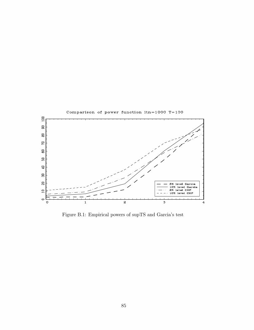
Figure B.1: Empirical powers of supTS and Garcia�s test

85

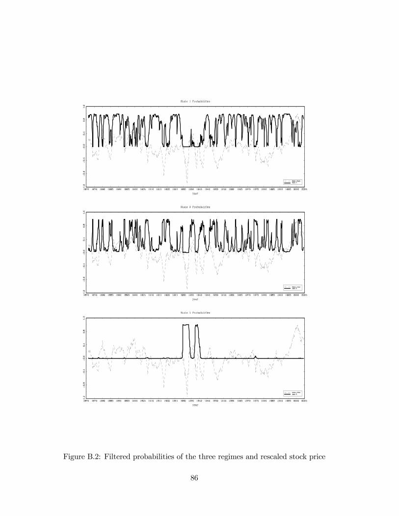
Figure B.2: Filtered probabilities of the three regimes and rescaled stock price

86