process modeling and optimization o. rodionova institute of chemical physics, moscow

April 19, 2023Samara WSC-5 1

Process Modeling and OptimizationProcess Modeling and Optimization O. Rodionova Institute of Chemical Physics, Moscow

MIR Space Station, Star City, Feb.17 2005


Based on PaperBased on Paper

Process control and optimization with simple interval calculation method

A. Pomerantseva, O. Rodionovaa, and A. Höskuldssonb

a Semenov Institute of Chemical Physics, Moscow, Russia

b Technical University of Denmark, Lyngby, Denmarkin print


OutlineOutline

Introduction

Real-world example – description

Passive optimization

Sic- in brief

Active optimization

Conclusions


PAT – a gift for chemometricsPAT – a gift for chemometrics((Process Analytical Technology)Process Analytical Technology)

FDA = U.S. Department of Health and Human Services Food and Drug Administration

Guidance for Industry PAT — A Framework for Innovative Pharmaceutical Development, Manufacturing, and Quality Assurance

Pharmaceutical CGMPs, September 2004

“MAN WITH THE GIFT” by Natar

Ungalaq


PAT ToolsPAT Tools

Multivariate tools for design, data acquisition and analysis

Process analyzers

Process control tools

Continuous improvement and knowledge management tools

(Guidance …)


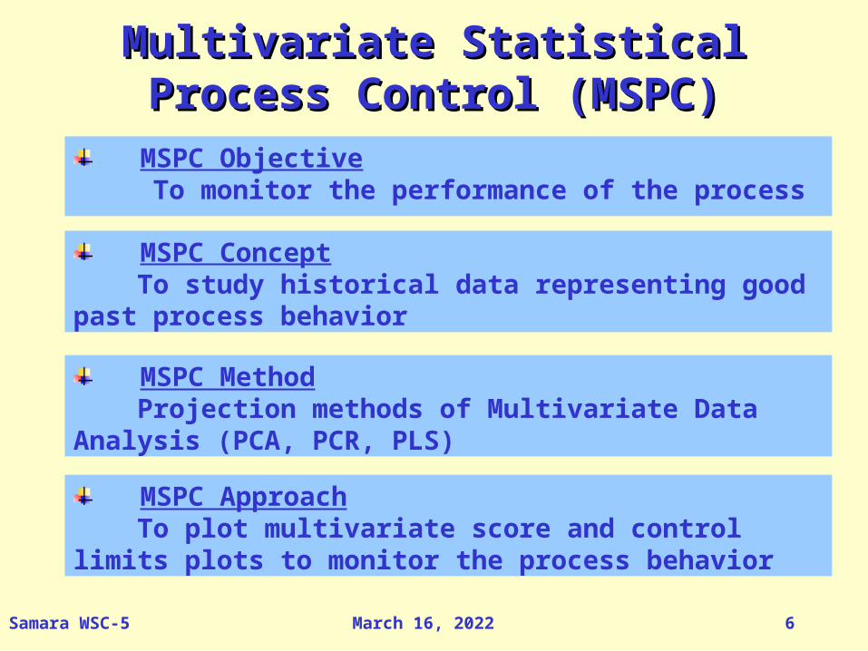
Multivariate Statistical Process Control Multivariate Statistical Process Control (MSPC)(MSPC)

MSPC Objective To monitor the performance of the process

MSPC Concept To study historical data representing good past process behavior

MSPC Method Projection methods of Multivariate Data Analysis (PCA, PCR, PLS)

MSPC Approach To plot multivariate score and control limits plots to monitor the process behavior


Multivariate Statistical Process Multivariate Statistical Process Optimization (MSPO)Optimization (MSPO)

MSPO Objective To optimize the performance of the process (product quality)

MSPO Concept To study historical data representing good past process behavior

MSPO Method Projection methods and Simple Interval Calculation (SIC) method

MSPO Approach To plot predicted quality at each process stage


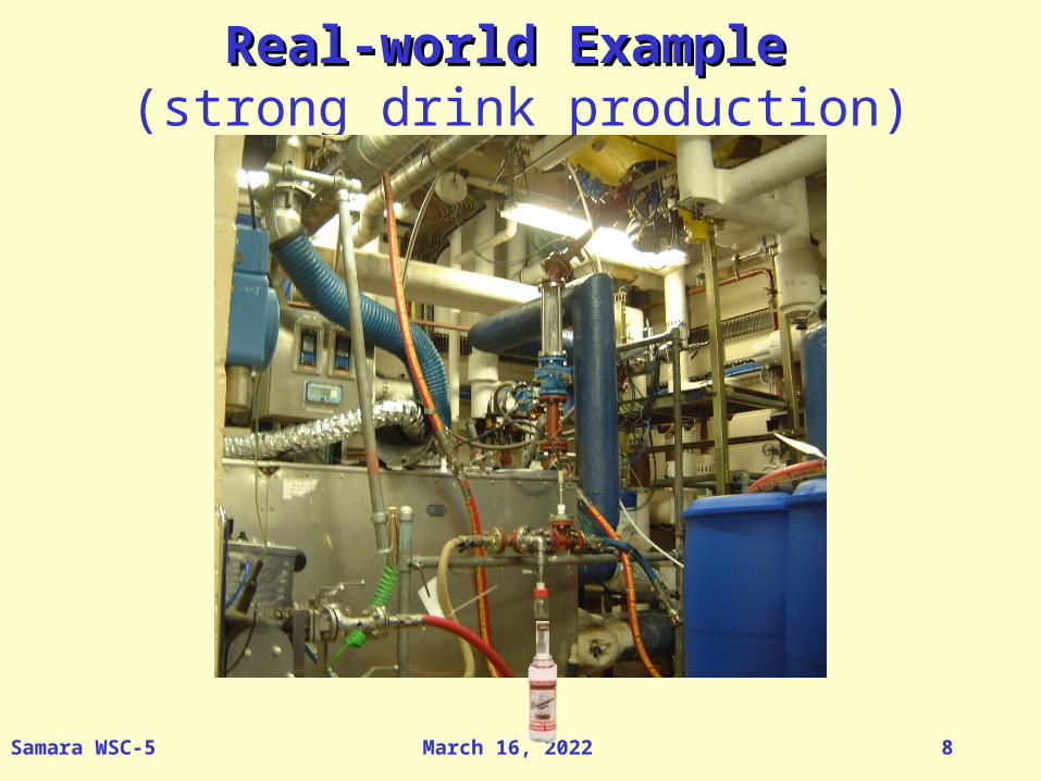
Real-world Example Real-world Example (strong drink production)


Technological Scheme. Multistage Process Technological Scheme. Multistage Process

S1 S2 S3

M1 M2 M3 CM1 CM2 CM3

W1 W2 W3 CW1 CW2 CW3

WR1 WR2

MR1 MR2

S

W CW

M CM PA1 A2 A3 A4 A5 A6

S1 S2 S3

M1 M2 M3 CM1 CM2 CM3

W1 W2 W3 CW1 CW2 CW3

WR1 WR2

MR1 MR2

S

W CW

M CM PA1 A2 A3 A4 A5 A6

I6

II8

III11

IV14

V16

VI19

VII25


Y preprocessing

Data Set DescriptionData Set Description

X preprocessing

S1

S2

S3

W1

W2

W3

WR

1

WR

2

CW

1

CW

2

CW

3

M1

M2

M3

MR

1

MR

2

CM

1

CM

2

CM

3

A1

A2

A3

A4

A5

A6 Y

Tra

inin

g

Se

t (1

02

)

Y

Tes

t S

et

(52

)

Y

XV XVI XVII

XI XII XIII XIV XV XVI XVII

XI XII XIII XIV


Quality Data (Standardized Y Set)Quality Data (Standardized Y Set)Training Set Samples

Lowest Quality Y=-1

Highest Quality Y=+1

-1.2

-0.8

-0.4

0.0

0.4

0.8

1.2

1 21 41 61 81 101

Y

Test Set Samples

Lowest Quality Y=-1

Highest Quality Y=+1

-1.2

-0.8

-0.4

0.0

0.4

0.8

1.2

1 11 21 31 41 51

Y


Overall PLS ModelOverall PLS Model

0

0.1

0.2

0.3

PC_0 PC_2 PC_4 PC_6 PC_8

PCs

RMSE Calbration

Validation

S1

S2

S3

W1

W2

W3

WR

1

WR

2

CW

1

CW

2

CW

3

M1

M2

M3

MR

1

MR

2

CM

1

CM

2

CM

3

A1

A2

A3

A4

A5

A6 Y

Y

YXTEST

XTRAINING

^

^PLS

6 PCs


Passive Optimization in PracticePassive Optimization in Practice

Thinker by Rodin


Main FeaturesMain Features

Objective To predict future process output being in the middle of the process

Concept To study historical data representing good past process behavior

Method PLS and Simple Interval Prediction

Approach Expanded Multivariate Process Modeling (E-MSPC)


Expanded Modeling. ExampleExpanded Modeling. ExampleS

1

S2

S3

W1

W2

W3 Y

Tra

inin

g

Se

t (1

02

)

Y

1 yxI XI

Sample 1, Normal Quality Insider

-1.0

-0.5

0.0

0.5

1.0 Y x10 PLS1

S1

S2

S3

W1

W2

W3

WR

1

WR

2

Y

Tra

inin

g

Se

t (1

02

)

Y

1 yxI xII

XI XII Sample 1, Normal Quality Insider

-1.0

-0.5

0.0

0.5

1.0 Y x10 PLS1

S1

S2

S3

W1

W2

W3

WR

1

WR

2

CW

1

CW

2

CW

3

Y

Tra

inin

g

Se

t (1

02

)

Y

1 y

xI xII xIII

XI XII XIII


-1.0

-0.5

0.0

0.5

1.0Y x10 PLS1

S1

S2

S3

W1

W2

W3

WR

1

WR

2

CW

1

CW

2

CW

3

M1

M2

M3 Y

Tra

inin

g

Se

t (1

02

)

Y

1 y

XIV

XI XII

xI xII xIII xIV

XIII


-1.0

-0.5

0.0

0.5

1.0Y x10 PLS1

S1

S2

S3

W1

W2

W3

WR

1

WR

2

CW

1

CW

2

CW

3

M1

M2

M3

MR

1

MR

2

Y

Tra

inin

g

Se

t (1

02

)

Y

1 y

XVXI XII XIII XIV

xVxI xII xIII xIV


-1.0

-0.5

0.0

0.5

1.0Y x10 PLS1

S1

S2

S3

W1

W2

W3

WR

1

WR

2

CW

1

CW

2

CW

3

M1

M2

M3

MR

1

MR

2

CM

1

CM

2

CM

3

Y

Tra

inin

g

Se

t (1

02

)

Y

1 y

XV XVI XI XII XIII XIV

xV xVI xI xII xIII xIV


-1.0

-0.5

0.0

0.5

1.0Y x10 PLS1

S1

S2

S3

W1

W2

W3

WR

1

WR

2

CW

1

CW

2

CW

3

M1

M2

M3

MR

1

MR

2

CM

1

CM

2

CM

3

A1

A2

A3

A4

A5

A6 Y

Tra

inin

g

Se

t (1

02

)

Y

1 yxV xVI xVIIxI xII xIII xIV

XV XVI XVIIXI XII XIII XIV


-1.0

-0.5

0.0

0.5

1.0Y x10 PLS1


Expanded PLS modelingExpanded PLS modeling

S1

S2

S3

W1

W2

W3

WR

1

WR

2

CW

1

CW

2

CW

3

M1

M2

M3

MR

1

MR

2

CM

1

CM

2

CM

3

A1

A2

A3

A4

A5

A6 Y

I

II

III

IV

V

VI

VII

I II III IV V VI VII0

0.04

0.08

0.12

0.16

Stage #

RMSE RMSEC RMSEP


Simple Interval Calculations (SIC) Simple Interval Calculations (SIC) in briefin brief

Triple Mobius by F. Brown


V —

V +

SIC main stepsSIC main steps

+


v +

v –

SIC-Residual and SIC-LeverageSIC-Residual and SIC-Leverage

Definition 2.

SIC-leverage is defined as –

This is a normalized precision

h

They characterize interactions between prediction and error intervals

y

y+

y–

Definition 1.

SIC-residual is defined as –

This is a characteristic of bias

r


Procedure Flow-ChartProcedure Flow-Chart

PLS/PCR model

Fixed number of PCs

Initial Data Set

{X,Y}

SIC-modeling

RESULTS

RESULTS

yhat

RMSEC RMSEP


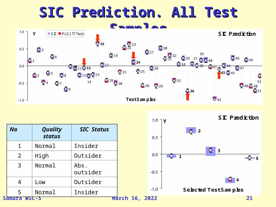
SIC Prediction. All Test SamplesSIC Prediction. All Test SamplesSIC Prediction

1

2

3

4

5

6

7

8

9

1011

12 15

17

18

19

20

21

2223

25

26

27

28

29

30

3132

33

34

35

38

40

41

42

44

45

46

47

48

49

5051

13

16

24

43

36

52

3739

14

-1.0

-0.5

0.0

0.5

1.0

Test Samples

Y SIC PLS1 Test SIC Prediction

1

2

3

4

5

6

7

8

9

1011

12 15

17

18

19

20

21

2223

25

26

27

28

29

30

3132

33

34

35

38

40

41

42

44

45

46

47

48

49

5051

14

3937

52

36

43

24

16

13

-1.0

-0.5

0.0

0.5

1.0

Test Samples

Y SIC PLS1 Test

SIC Prediction

5

4

31

2

-1.0

-0.5

0.0

0.5

1.0

Selected Test Samples

Y

No Quality status SIC Status

1 Normal Insider

2 High Outsider

3 Normal Abs. outsider

4 Low Outsider

5 Normal Insider


Expanded ModelingExpanded Modeling PLS + SICPLS + SICS

1

S2

S3

W1

W2

W3 Y

Tra

inin

g

Se

t (1

02

)

Y

1 yxI XI


-1.0

-0.5

0.0

0.5

1.0 SIC PLS1

Y x1

S1

S2

S3

W1

W2

W3

WR

1

WR

2

Y

Tra

inin

g

Se

t (1

02

)

Y

1 yxI xII

XI XII Sample 1, Normal Quality Insider

-1.0

-0.5

0.0

0.5

1.0 SIC PLS1

Y x1

S1

S2

S3

W1

W2

W3

WR

1

WR

2

CW

1

CW

2

CW

3

Y

Tra

inin

g

Se

t (1

02

)

Y

1 y

xI xII xIII

XI XII XIII


-1.0

-0.5

0.0

0.5

1.0 SIC PLS1

Y x1

S1

S2

S3

W1

W2

W3

WR

1

WR

2

CW

1

CW

2

CW

3

M1

M2

M3 Y

Tra

inin

g

Se

t (1

02

)

Y

1 yxI xII xIII xIV XI XII XIII XIV


-1.0

-0.5

0.0

0.5

1.0 SIC PLS1

Y x1

S1

S2

S3

W1

W2

W3

WR

1

WR

2

CW

1

CW

2

CW

3

M1

M2

M3

MR

1

MR

2

Y

Tra

inin

g

Se

t (1

02

)

Y

1 yxVxI xII xIII xIV

XVXI XII XIII XIV Sample 1, Normal Quality Insider

-1.0

-0.5

0.0

0.5

1.0 SIC PLS1

Y x1

S1

S2

S3

W1

W2

W3

WR

1

WR

2

CW

1

CW

2

CW

3

M1

M2

M3

MR

1

MR

2

CM

1

CM

2

CM

3

Y

Tra

inin

g

Se

t (1

02

)

Y

1 yxV xVI xI xII xIII xIV

XV XVI XI XII XIII XIV


-1.0

-0.5

0.0

0.5

1.0 SIC PLS1

Y x1

S1

S2

S3

W1

W2

W3

WR

1

WR

2

CW

1

CW

2

CW

3

M1

M2

M3

MR

1

MR

2

CM

1

CM

2

CM

3

A1

A2

A3

A4

A5

A6 Y

Tra

inin

g

Se

t (1

02

)

Y

1 y

XV XVI XVIIXI XII XIII XIV

xV xVI xVIIxI xII xIII xIV


-1.0

-0.5

0.0

0.5

1.0 SIC PLS1

Y x1


Expanded SIC modelingExpanded SIC modeling

VIIVIVIVIIIIII0

0.2

0.4

0.6

0.8

1

Stage #

bmin bsic w


Samples 2 & 3Samples 2 & 3Sample 2, High Quality, Outsider

-1.0

-0.5

0.0

0.5

1.0

x2 SIC

PLS1 Y

Sample 3, Normal Quality, Absolute Outsider

-1.0

-0.5

0.0

0.5

1.0

x3 SIC

PLS1 Y


Samples 4 & 5Samples 4 & 5Sample 4, Low Quality, Outsider

-1.0

-0.5

0.0

0.5

1.0 x4 SIC

PLS1 Y

Sample 5, Normal Quality, Insider

-1.0

-0.5

0.0

0.5

1.0x5 SIC

PLS1 Y


S1

S2

S3

W1

W2

W3

WR

1

WR

2

CW

1

CW

2

CW

3

M1

M2

M3

MR

1

MR

2

Y

Tra

inin

g

Se

t (1

02

)

Y

10 xI xII xIII xIV

XVXI XII XIII XIV

Passive Optimization. StagePassive Optimization. Stage VV

? ?

Decision MR1 MR2

0 -0.25 0.08

1 0.00 0.00

2 -0.23 0.10

3 -0.04 0.18

4 0.13 0.27

PLS/SICprediction

3 -0.04 0.18

Прогноз качества, y

43210-1.0

-0.5

0.0

0.5

1.0

Решения

Prediction of y


The Necessity of Active The Necessity of Active OptimizationOptimization

F. Yacoub, J.F. MacGregor Product optimization and control in the latent variable space of nonlinear PLS models. Chemom. Intell. Lab. Syst 70:63-74, 2004

B.-H. Mevik, E. M. Færgestad, M. R. Ellekjær, T. Næs Using raw material measurements in robust process optimization Chemom. Intell. Lab. Syst 55:135-145, 2001

A. Höskuldsson Causal and path modelling. Chemom. Intell. Lab. Syst., 58: 287-311, 2001


Active Optimization in PracticeActive Optimization in Practice

“Let Us Beat Our Swords into Ploughshares” by Vuchetich’


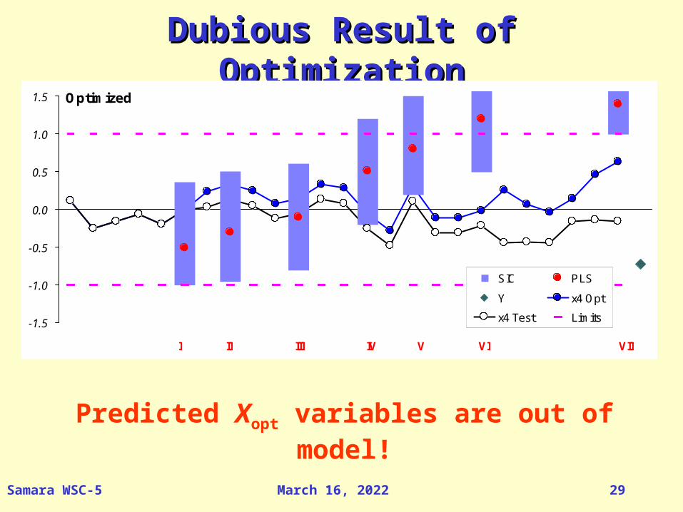
Dubious Result of OptimizationDubious Result of OptimizationOptimized

III III IV V VI VII

-1.5

-1.0

-0.5

0.0

0.5

1.0

1.5

Y x4 Opt

x4 Test

Optimized

VIIVIVIVIIII II

-1.5

-1.0

-0.5

0.0

0.5

1.0

1.5

SIC PLS

Y x4 Opt

x4 Test

Optimized

III III IV V VI VII

-1.5

-1.0

-0.5

0.0

0.5

1.0

1.5

SIC PLS

Y x4 Opt

x4 Test Limits

Predicted Xopt variables are out of model!


Main FeaturesMain Features

Objective To find corrections for each process stage that improve the future process output (product quality)

Concept Corrections are admissible if they are similar to ones that sometimes happened in the historical data in the similar situation

Method PLS1, PLS2, SIC

Approach Multivariate Statistical Process Optimization (MSPO)


X Z y

x z =? y =?

b t c t

PLS1

PLS2

y =xb +zc^

PLS1 XY: (X,Z) y

Intermediate StageIntermediate Stage

The Scheme of Three Data Block Modeling

X Z y

x z =? y =?

PLS2 XZ: X Z

X Z y

x z =? y =?

b t c t

Dt

PLS1

PLS2

y =xb +zc^z =x D^


Optimization ProblemOptimization ProblemStage I XI

W1, W2, W3 ,S1, S2, S3PLS1 Quality measure

YStage II XII

WR1,WR2

Fixed variables Xfix

PLS1 Quality measure Y

Optimized Z

Y = X*a = Xfix b+ Z*c, where a =b+c

Model

For new (x,z) maximize(xtb+ztc) w.r.t. z, z Lz

Task

max (y) = Xfix b + max (zt)*c, as all a > 0 (by factor)

Solution


Linear Optimization Linear Optimization Linear function always reaches extremum at the border.

So, the main problem of linear optimization is not to find a

solution, but to restrict the area, where this solution should

be found.

x

y=a*x

x

y=a*x

x

y=a*x

x

y=a*x


Optimization restrictionsOptimization restrictions

I. All process and quality variables should be inside predefined control limits.

|xi|1 and |yj|1 for every i,j

II. Adjusted variables should not contradict process model

For new (x,z) maximize(xtb+ztc) w.r.t. z, z LzLz


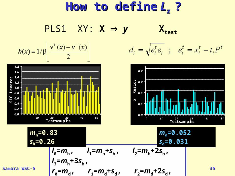
How to defineHow to define L Lz z ??

l0=mh, l1=mh+sh, l2=mh+2sh, l3=mh+3sh,

r0=md, r1=md+sd, r2=md+2sd, r3=md+3sd,

PLS1 XY: X y Xtest

mh=0.83 sh=0.26 md=0.052 sd=0.031

0.0

0.2

0.4

0.6

0.8

1.0

1.2

1.4

1.6

1.8

10 20 30 40 50Test samples

SIC

Le

ve

rag

e

0.0

0.1

0.1

0.2

0.2

1 11 21 31 41 51Test samples

x R

es

idu

al


z1i

z2i

-0.075

-0.025

0.025

0.075

z1 i

z2 i

-0.075

-0.025

0.025

0.075

z1i

z2i

-0.075

-0.025

0.025

0.075

Three optimization strategiesThree optimization strategies

X Z y

x z =? y =?

b t c t

Dt

PLS1

PLS2

y =xb +zc^z =x D^

z1i

z2i

-0.075

-0.025

0.025

0.075

PLS2 XZ: X Z

z1i

z2i

-0.075

-0.025

0.025

0.075


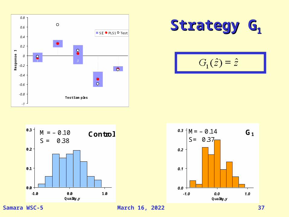
Strategy GStrategy G11

Control

0.0

0.1

0.2

0.3

-1.0 0.0 1.0Quality, y

M = – 0.10S = 0.38

G1

0.0

0.1

0.2

0.3

-1.0 0.0 1.0Quality, y

M= – 0.14S= 0.37

-1

-0.8

-0.6

-0.4

-0.2

0

0.2

0.4

0.6

0.8

1 2 3 4 5

Test Samples

Res

po

nse

1

SIC PLS1 Test


Sample 5 Normal Quality Insider (GSample 5 Normal Quality Insider (G33))Test

VIIVIVIVIIIIII

-1.0

-0.5

0.0

0.5

1.0S

1

S2

S3

W1

W2

W3

WR

1

WR

2

CW

1

CW

2

CW

3

M1

M2

M3

MR

1

MR

2

CM

1

CM

2

CM

3

A1

A2

A3

A4

A5

A6 Y

Optimized

VIIVIVIIIIII IV

-1.0

-0.5

0.0

0.5

1.0

S1

S2

S3

W1

W2

W3

WR

1

WR

2

CW

1

CW

2

CW

3

M1

M2

M3

MR

1

MR

2

CM

1

CM

2

CM

3

A1

A2

A3

A4

A5

A6 Y


Sample 3 Normal Quality Abs. Outsider (GSample 3 Normal Quality Abs. Outsider (G33))Test

VIIVIVIVIIIIII

-1.0

-0.5

0.0

0.5

1.0S

1

S2

S3

W1

W2

W3

WR

1

WR

2

CW

1

CW

2

CW

3

M1

M2

M3

MR

1

MR

2

CM

1

CM

2

CM

3

A1

A2

A3

A4

A5

A6 Y

Optimized

VIIVIVIIIIII IV

-1.0

-0.5

0.0

0.5

1.0

S1

S2

S3

W1

W2

W3

WR

1

WR

2

CW

1

CW

2

CW

3

M1

M2

M3

MR

1

MR

2

CM

1

CM

2

CM

3

A1

A2

A3

A4

A5

A6 Y


Sample 4 Low Quality Outsider (GSample 4 Low Quality Outsider (G33))Test

I II III IV V VI VII

-1.0

-0.5

0.0

0.5

1.0S

1

S2

S3

W1

W2

W3

WR

1

WR

2

CW

1

CW

2

CW

3

M1

M2

M3

MR

1

MR

2

CM

1

CM

2

CM

3

A1

A2

A3

A4

A5

A6 Y

Optimized

IVI II III V VI VII

-1.0

-0.5

0.0

0.5

1.0

S1

S2

S3

W1

W2

W3

WR

1

WR

2

CW

1

CW

2

CW

3

M1

M2

M3

MR

1

MR

2

CM

1

CM

2

CM

3

A1

A2

A3

A4

A5

A6 Y


Results of Optimization. Results of Optimization. Quality variable Quality variable

Control

0.0

0.1

0.2

0.3

-1.0 0.0 1.0Quality, y

M = – 0.10S = 0.38

G2

0.0

0.1

0.2

0.3

-1.0 0.0 1.0Quality, y

M = 0.23S = 0.36

G3

0.0

0.1

0.2

0.3

-1.0 0.0 1.0Quality, y

M = 0.55S = 0.35

G1

0.0

0.1

0.2

0.3

-1.0 0.0 1.0Quality, y

M= – 0.14S= 0.37


Results of Optimization Results of Optimization

Opt. strategy h l 0 l 0<h l 1 l 1<h l 2 l 2<h l 3 h >l 3 m h s h

Control 26 19 5 2 0 0.835 0.261G1 36 12 3 1 0 0.723 0.277G2 28 17 5 1 1 0.809 0.305G3 26 11 10 5 0 0.854 0.385

Distribution of the SIC leverages, h for the different optimization strategies.

Opt. strategy d r 0 r 0<d r 1 r 1<d r 2 r 2<d r 3 d >r 3 m d s d

Control 26 17 9 0 0 0.052 0.031G1 35 10 3 4 0 0.047 0.03G2 19 25 5 3 0 0.068 0.024G3 0 9 29 10 4 0.105 0.027

Distribution of the root mean squared X residuals, d for the different strategies


ConclusionsConclusions

Application of the series of expanding PLS/SIC models helps to predict the effect of planned actions on the product quality, and thus enables passive quality optimization.

The presented optimization methods are based on the PLS block modeling as well as on the Simple Interval Calculation

For active optimization: (1) No improvement in quality obtained “inside” the model; (2) To yield a considerable improvement in y, the optimized variable values should be located in the boarder of the model; (3) It is obligatory to verify that optimized values do not contradict the process history.

process modeling and optimization o. rodionova institute of chemical physics, moscow

Documents

process stagesamara

process behaviorsamara

rodinsamara wsc

brownsamara wsc

modelingsamara wsc

examplesamara wsc

multistage process samara

main stepssamara wsc