process flexibility revisited: the graph expander and its applications

Process Flexibility Revisited: The Graph Expanderand Its Applications

Mabel C. ChouDepartment of Decision Sciences, NUS Business School. Email: [email protected]

Chung-Piaw TeoDepartment of Decision Sciences, NUS Business School. Email: [email protected]

Huan ZhengManagement Science Department, Shanghai Jiao Tong University. Email: [email protected]

We examine how a flexible process structure might be designed to allow the production system to better

cope with fluctuating supply and demand, and to match supply with demand in a more effective manner.

We argue that good flexible process structures are essentially highly connected graphs, and use the concept

of graph expansion (a measure of graph connectivity) to achieve various insights into this design problem.

A number of design guidelines are well known in the literature. Principles such as “a long chain performs

better than many short chains,” and that one should “try to equalize the number of plants (resp. products),

measured in total units of capacity (resp. mean demand), which each product (resp. plant) in the chain is

directly connected to,” can now be interpreted from this new angle as a development of different ways in

which the underlying network can achieve a good expansion ratio. The same principle extends to other new

design guidelines - trying to equalize the number of plants (measured in total number of units) assigned to

each pair (or even triplet) of products, or vice versa, can also help the decision maker to arrive at a good

process structure.

We analyze the worst-case performance of the flexible design problem under a more general setting,

which encompasses a large class of objective functions. We show that whenever demand and supply are

balanced and symmetrical, the graph expander structure (a highly connected but sparse graph) is within ǫ

optimality of the fully flexible system, for all demand scenarios, although it uses a far smaller number of

links. Furthermore, the same graph expander structure works uniformly well for all objective functions in

this class.

Based on this insight, we develop a simple and easy-to-implement heuristic to design flexible process

structure. Numerical results show that this heuristic performs well for a variety of numerical examples

previously studied in the literature. We also use this idea on a set of real data obtained from a bread delivery

system in Singapore, with the goal of minimizing the excess amounts of bread brought to each location.

1. Introduction

The wave of economic reforms and globalization around the world has led to a much more complex

operational environment for many manufacturers. Increased reliance on make-to-order fulfillment

systems means that manufacturers can no longer hedge against demand variability with finished

1

Author: Article Short Title

2

goods inventory. This necessitates a search for new production strategies that can help manufac-

turers to cope with an increasingly volatile environment.

Indeed, flexibility, defined as the ability of a system to respond or react to a change with little

penalty in time, effort, or cost (Upton, 1994), is a strategic competitive option that many manufac-

turers are beginning to embrace. In the automobile industry, for example, companies are moving

from focused factories to flexible factories. The Ford Motor Company, for instance, invested $485

million in two Canadian engine plants to renovate and retool them with a flexible system. It has

also launched a plan to equip most of its 30-odd engine and transmission plants all over the world

with flexible systems. Similar initiatives to make plants more flexible have also been launched in

companies like GM and Nissan. These initiatives are viewed as crucial to the survival of automobile

manufacturers in the increasingly competitive global environment.

The effectiveness of a flexibility strategy of this kind is highly dependent on two factors: (i)

The relationship between the total invested capacity and the (random) external demand, and (ii)

the design of the flexible process structure. The first issue concerns the optimal capacity to invest

in, considering the cost of investment and the uncertainty of demand. The second issue revolves

around how the invested capacity should be allocated among different plants, as well as how much

and what types of production capability should be configured in each plant. The focus of this paper

is on the second issue.

A plant is considered more flexible if it can use its equipment and resources to produce more

types of product. However, how these capabilities are allocated among the plants can also affect

the system’s ability to handle the demand for the different products. In this setting, the focus is to

design a process structure to handle as much demand as possible, or to maximize the utilization of

the equipment in the plants. Our interest in the problem, however, comes from a slightly different

source. It is motivated by the operation of a new charity organization based in Singapore, where

the focus is on ensuring that the donations received go into the right hands - the hands of those

people in the homes supported by the organization (cf. Lee (2004)). Interestingly, as the mission of

the program is to save food, our objective here is to design a process structure to minimize waste

(above the requirement); that is, the excess amount of donated food brought to the homes.

The logistical concept used in the delivery operation is amazingly simple. Each bakery is served

by one volunteer each night to bring the donated bread to the designated home. An administrator

for the Food From the Heart (FFTH) program will select routes (bakery-home assignment) and

assign a volunteer (based on the address of the volunteer, and the mode of transport he or she uses)

to each route. To reduce the burden on the volunteers, the administrator usually assigns a fixed


3

route to each volunteer1. While the assignment policy adopted by FFTH significantly reduces the

complexity of the operation, the embedded rigidity inevitably introduces an unintended problem in

the operation - the mismatch between the supply (the amount of donated bread) and the demand

(the amount required at each home). This problem is exacerbated by the fact that the supply from

each bakery on each night is random since it depends on the amount of bread produced and sold

by the bakery. It is ironic, as pointed out by one volunteer, that a program with the aim of saving

food will end up with the donated bread being thrown away, or consumed by a third party.

One way to minimize wastage is to have a synchronized delivery system, where the allocation

of bread to homes is only determined upon the realization of the random supplies, and where one

or several volunteers can then split the donations collected at a bakery between several homes. It

is obvious that a “full flexibility system” which allows the bread from each bakery to be sent to

any home will best match the supply and the demand. But such a system is also cumbersome to

manage and utilizes too many volunteers. We therefore aim to design a simpler flexible routing

structure for the system, where the bread from each bakery can only be brought to a small number

of predesignated homes. Note that our objective here is different. Since the total supply is normally

smaller than the total requirement in our system, the challenge here is to minimize the “excess”

supply (i.e., above the requirement) brought to each home, to ensure that no donated food will go

to waste.

The earlier studies on process flexibility basically produced two important insights. First, these

studies showed that if we add additional flexibility to a rigid system in the right places (say, by

allowing a plant to produce one more type of product), a significant improvement in the sys-

tem’s performance can be expected. Some studies (e.g. Jordan and Graves (1995)) even provided

examples showing that a very sparse partial flexibility system can be nearly as effective as a full

flexibility system (where all the plants can be used to produce all types of product). Second, on

the question of where flexibility should be added, these studies suggested that it should be added

to create fewer and longer chains, where a “chain” is a group of products and plants which are all

connected, directly or indirectly, by product assignment decisions. A long chain is preferred when

designing a flexibility structure because it pools more plants and products and thus deals with

uncertainty more effectively than a short chain. The effectiveness of the chaining strategy has been

validated by many simulation studies in different areas, ranging from manpower training to call

center staffing (cf. Jordan and Graves (1995), Hopp et al. (2004), Iravani et al. (2005)).

1 So that each volunteer only needs to be familiar with one route; that is, from a bakery to a home.


4

The chaining concept Jordan and Graves (1995) is arguably the most influential strategy used

in practice to design good process structure. However, beyond the long chain, little is known about

the nature of a good process structure, especially for more general cases, such as when not all

products and plants have the same level of mean demand and capacity. Indeed, when Jordan and

Graves (1995) stated three general design principles, they also mentioned that they had no firm

guidelines for adding flexibility for more general cases. That is, these design principles alone do not

provide an implementable heuristic which can be used to design a process structure in all settings.

In fact, they used the principles to develop numerous structures, and used numerical simulations

to estimate the performances (average lost sales and unused capacity for each product and at each

plant) of each structure in order to obtain the best-of-class process structure. As explained later,

our paper tries to address this issue by providing a simple and implementable heuristic to produce

a good flexible process structure.

Our main contribution in this paper is to analyze this problem from a new perspective. In

previous literature, only the average performance objectives were studied. In this paper, we analyze

the performance of a sparse structure under the worst-case setting to ensure that our performance

level can always be achieved. In addition, we generalize the model so that we can also handle

objective functions such as waste minimization, as encountered in the FFTH program. We introduce

the concept of graph expansion, which is widely used in the area of graph theory and computer

science, to analyze the performance of the flexible process structure. Under a mild assumption, we

show that the class of graph expander (highly connected graphs) works extremely well for a large

class of objective functions, despite the fact that it uses a far smaller number of links compared

with the full flexibility system. In fact, for many classes of demand functions, we can show that

the performance of 2-chain is identical to the performance of the fully flexible system. This result

is considerably stronger than the current known result on the average performance of 2-chain vis-

a-vis the fully flexible system. Finally, we use the new insight obtained from our study on graph

expansion to develop new design guidelines which lead to a simple and implementable heuristic to

produce a good flexible process structure.

The rest of the paper is organized as follows. In Section 2, we review the related literature on

process flexibility. In Section 3, we present a general framework for the process structure design

problem, encompassing both the FFTH model and the classical process flexibility model as special

cases. We analyze the performance of the graph expander within our framework, when supply and

demand are balanced and identical. In Section 4, we develop new design guidelines and a simple

heuristic to develop good process structures for the general case when demand and supply may


5

not be identical or balanced. In Section 5, we conduct an extensive numerical study to compare

the performance of our heuristic with existing benchmarks, where the objective is to maximize

the amount of production. We also test the performance of the heuristic on a system where the

objective is to minimize waste, using the data from the FFTH program. We show that our heuristic

leads to a good flexible routing system, which would dramatically decrease the food wastage in the

program. Finally, we provide some concluding remarks in Section 6.

2. Literature Review

Research on issues related to flexibility has a broad scope. Sethi and Sethi (1990) conducted an

extensive survey of the applications of flexibility in different areas. They categorized 11 types of

flexibility, including “machine flexibility,” “product flexibility,” “routing flexibility,” and “resource

flexibility.” There is by now a vast literature in each category. Jack and Raturi (2003) studied the

impact of “volume flexibility” in detail. In addition, Shi and Daniels (2003) surveyed the literature

relating to “e-business flexibility,” which is a new area in flexibility research. They reviewed the

process flexibility literature that dealt with e-business issues and defined the concept of “e-business

flexibility” in their paper.

The classic study on process flexibility was conducted by Jordan and Graves (1995). Their

findings were based on their study of General Motors’ production process. Because market condi-

tions change quickly, customers’ demand for different models is very unpredictable. The traditional

“one-plant, one-model” process cannot adequately cope in this environment - demand for some

models cannot be fully satisfied due to capacity limitations, whereas some plants may have spare

capacity due to insufficient demand. They proposed changing the traditional focused operation to

a more flexible one, where one plant can produce a multiple number of models. In this way, the

company can use the invested capacity in the plants to handle demand variations across models in

a more effective manner.

The ideal design is the full flexibility system, where every plant is able to produce any product.

But this is too costly, and each plant needs to have the tooling capability to produce every model.

In their paper, Jordan and Graves (1995) observed (using simulations) that the partial flexibility

structure, where one plant can produce only a limited number of models (suitably selected), can

accrue most of the benefits offered by the full flexibility system. They further proposed a “chaining”

strategy as a managerial guideline for the design of a flexibility structure.

Aksin and Karaesmen (2007) applied network theories to the study of flexible structure. The

flexibility of a system is determined by the maximum network flow through customer demand to


6

the manufacturers. They carefully studied the symmetrical flexible system and derived the sub-

modularity property of the flexibility structure. The authors derived the concavity of certain fixed

process structures, as a function of the degree of each production node (the number of models each

plant can handle). The returns from added flexibility into the system is thus diminishing.

Chou et al. (2007) demonstrated this effect more succinctly by comparing the performance of

the chaining structure with the fully flexible system for an asymptotically large system. A k-chain

(denoted by Ck) is a subgraph in an n by n bipartite graph where each supply node i is linked to

demand nodes i, i + 1, . . . , i + k − 1 (modulo n). When the demand for each product is uniformly

distributed between 0 and 2C, and each plant has a capacity of C units, they showed a surprising

result that the performance of a 2-chain is already close to 89.6% of that attained by a fully

flexible system when the size of the system is asymptotically large. The performance in the case of

normal distribution is even more impressive. By replacing the uniform distribution with a normal

distribution N(C,σ2), with C = 3σ, the performance of a 2-chain is at an impressive level of 96%

when the system is asymptotically large.

Many subsequent works extended the chaining strategy and partial flexibility concept and pro-

vided important observations and insights in various areas such as the supply chain (cf. Graves and

Tomlin (2003), Bish et al. (2005)), flexible workforce scheduling (cf. de Farias and Van Roy (2004),

Hopp et al. (2004)), and queuing (cf. Benjafaar (2002), Gurumurthi and Benjaafar (2004)). For

example, Graves and Tomlin (2003) extended Jordan and Graves (1995) to obtain flexibility

guidelines for multistage supply chains. On the other hand, Bish et al. (2005) cautioned that

certain practices that might seem reasonable in a flexible system would lead to greater swings in

production, resulting in higher operational costs, and might reduce profits. Iravani et al. (2005)

proposed a new perspective on process flexibility. They used the concept of “structural flexibility”

to evaluate a system’s process capability. They created an n by n “structural flexibility matrix” (SF

Matrix) to study the flexibility of a cross-training CONWIP (CONstant Work-In-Process) system.

They used the mean of all the elements in the SF Matrix and the dominant eigenvalue as indices

of flexibility.

3. The Process Flexibility Problem

We use a bipartite graph to represent flexibility structures. On the left is a set A of n product

nodes while on the right is a set B of m facility/plant nodes. A link connecting product node i

to facility node j means that facility j has the capability to produce product i. Let F ⊆ A×B =

(i, j) : i ∈ A, j ∈ B denote the set of all such links; that is, the edge set of the bipartite graph.

Hence, each flexibility configuration can be uniquely represented by a bipartite graph F .


7

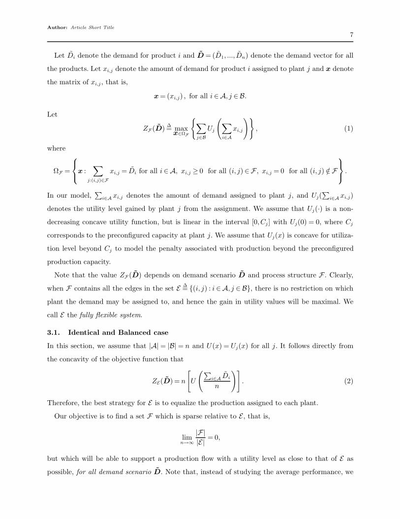
Let Di denote the demand for product i and D = (D1, ..., Dn) denote the demand vector for all

the products. Let xi,j denote the amount of demand for product i assigned to plant j and x denote

the matrix of xi,j , that is,

x = (xi,j) , for all i∈A, j ∈B.

Let

ZF(D)∆= max

x∈ΩF

∑

j∈B

Uj

(

∑

i∈A

xi,j

)

, (1)

where

ΩF =

x :∑

j:(i,j)∈F

xi,j = Di for all i∈A, xi,j ≥ 0 for all (i, j)∈F , xi,j = 0 for all (i, j) /∈F

.

In our model,∑

i∈A xi,j denotes the amount of demand assigned to plant j, and Uj(∑

i∈A xi,j)

denotes the utility level gained by plant j from the assignment. We assume that Uj(·) is a non-

decreasing concave utility function, but is linear in the interval [0,Cj] with Uj(0) = 0, where Cj

corresponds to the preconfigured capacity at plant j. We assume that Uj(x) is concave for utiliza-

tion level beyond Cj to model the penalty associated with production beyond the preconfigured

production capacity.

Note that the value ZF(D) depends on demand scenario D and process structure F . Clearly,

when F contains all the edges in the set E∆= (i, j) : i ∈A, j ∈ B, there is no restriction on which

plant the demand may be assigned to, and hence the gain in utility values will be maximal. We

call E the fully flexible system.

3.1. Identical and Balanced case

In this section, we assume that |A| = |B| = n and U(x) = Uj(x) for all j. It follows directly from

the concavity of the objective function that

ZE(D) = n

[

U

(

∑

i∈A Di

n

)]

. (2)

Therefore, the best strategy for E is to equalize the production assigned to each plant.

Our objective is to find a set F which is sparse relative to E , that is,

limn→∞

|F|

|E|= 0,

but which will be able to support a production flow with a utility level as close to that of E as

possible, for all demand scenario D. Note that, instead of studying the average performance, we


8

aim to find a sparse structure which performs well even under the worst-case demand scenario.

We say that F is within ǫ optimality of E if

ZF(D)≥ (1− ǫ)ZE(D)

for all demand scenario D.

We develop next a general framework for the process flexibility design problem, assuming that

supply and demand are identical; that is, we assume that the demand Di for product i is identically

distributed with mean µ, and that the capacity of each plant is configured at constant µ.

Note that we impose no further structure on U(x) beyond µ, except for concavity. U(x) can be

used to model the utility value accrued in the plant when the demand assigned is x. When x is

within the preconfigured capacity level, the growth in the utility function is linear, but beyond that,

there may be decreasing marginal utility for each extra unit. Examples of such utility functions

include:

• U(x) = min(x,µ). Here, the plant does not gain any additional utility for production beyond

µ. This models the situation when there is no emergency backup option, so that all demand beyond

µ will be lost.

• U(x) = min(x,p + (µ− p)x/µ). Here, the plant loses a profit margin of p/µ for each unit of

production beyond µ.

When U(x) = min(x,µ), where µ = E(Di), our problem reduces to the classical plant-product

process design problem. A structure such as a 2-chain (denoted by C2) is known to work extremely

well for this case.2 In fact, asymptotically, it can be shown (cf. Chou et al. (2007)) that

E

(

ZC2(D)

n

)

≈ 0.96×E

(

ZE(D)

n

)

for large n,

when Di’s are independent normal random variables with mean µ, standard deviation σ = µ/3,

truncated in the range [0,2µ]. This surprising feature is desirable, because C2 uses a much smaller

number of arcs compared to E .

The performance of the process structure depends strongly on the variability of the demand. To

the best of our knowledge, there are very few studies which take into account the impact of the

variance and correlational structure of the uncertain parameters. If the variance can be arbitrarily

large, then it is conceivable that a sparse process flexibility structure may be much less effective

than a fully flexible structure, as demonstrated by the following example.

2 A k-chain (denoted by Ck) is a subgraph in an n by n bipartite graph where each supply node i is linked to demandnodes i, i + 1, . . . , i + k− 1 (modulo n).


9

Example 1. Consider a system with n unit capacity nodes and n demand nodes, where Dj = n

with probability 1/n and Dj = 0 with probability 1 − 1/n, for j = 1,2, . . . , n. Furthermore, the

demands are correlated in such a way that∑n

j=1 Dj = n for all realizations; in other words, exactly

one demand node has a value of n and all other n− 1 demand nodes have a value of 0. Assume

U(x) = min(x,1). For any given D, it is easy to see that in the fully flexible system, ZE(D) = n.

On the other hand, in any partially flexible system F with a degree of flexibility bounded by some

fixed k (i.e., each demand node has at most k neighbors), ZF(D) is at most k, which is much

smaller than ZE(D) for a sparse process flexibility structure.

To rule out such extreme cases, in the rest of the paper we assume that the demand satisfies the

following condition:

Assumption: Di ≤ λE[Di] for some constant λ almost surely.

For the ease of reference, we define the following:

Definition 1. Di has a bounded variation of λ if the above assumption is satisfied.

It turns out that when demand has a bounded variation, we can prove that, for any given ǫ > 0

and sufficiently large n, there is a type of process structure F , using only a sparse number of edges,

with

ZF(D)≥ (1− ǫ)ZE(D)

for all D satisfying the bounded variation condition. Intuitively, the near optimal process structure

F identified in this paper has very few edges, but has very high connectivity with many paths

linking different pairs of nodes in A ∪ B, thus allows us to effectively allocate capacities to the

demands. To gain this intuition, we need to understand the notion of graph connectivity associated

with every process structure.

Definition 2. A structure F is k-connected if there are at least k node disjoint paths linking

every pair of nodes in A∪B.

There is a clear trade-off between the level of connectivity and the number of edges - for higher

graph connectivity, the structure needs to have more edges. A k-chain denoted by Ck is clearly k-

connected with kn edges. However, while C2 is the only 2-connected graph with 2n edges, there are

exponentially many classes of k-connected graphs with kn edges, for k > 2. In particular, there is

a class of highly connected graphs, called the graph expander, which has received a lot of attention

in the literature. The “expander” concept was first introduced by Bassalygo and Pinsker (1973)

in a study of communication networks. Basically, graph expanders are graphs where every “small”

subset of nodes is linked to a large neighborhood, thus allow effective allocation of capacities

to the demands. The ratio of the size of the neighborhood and the size of the subset measures


10

the expansion capability of the graph. We define the neighborhood of a subset and the “graph

expander” concept formally in the following:

Definition 3. Let F be a bipartite graph with partite sets A and B. For S ⊆A, the neighbor-

hood of S in F is defined as

ΓF(S)∆= j ∈ B : (i, j)∈F for some i∈ S .

For simplicity of notation, we drop F and denote the neighborhood of S as Γ(S) when there is no

ambiguity about which F is being considered.

Definition 4. Let F be a bipartite graph with partite sets A and B. The structure F is an

(α,λ,∆)-expander if

• for every v ∈A, deg(v)≤ ∆, and

• for all small subsets S ⊂A with |S| ≤ αn, we have

|Γ(S)| ≥ λ|S|.

Remarks:

1. For a n × n bipartite graph which is also an (α,λ,∆)-expander, the number of edges is at

most ∆n.

2. A 2-chain C2 is clearly a ( 1n,2,2)-expander, since for each subset of size 1, there are at least

two neighbors. Furthermore, the degree is bounded by 2. It is also a ( 2n,1.5,2)-expander, since for

every subset S of size at most 2, |Γ(S)| ≥ 1.5|S|. It is easy to check that it is simultaneously a

( kn, (k +1)/k,2)-expander, for all k ≤ n− 1.

3. A graph expander ensures that any suitably small group of product nodes is connected to a

relatively large number of plants, thus works well in matching supply and demand as we will show

in Theorem 1. Moreover, the notion that a long chain is better than a short chain can be cast in

the same light: the expansion ratios for “small” subsets of product nodes in long chains are higher

than those in short chains.

Theorem 1. Consider an n × n system, where the demand Di has a bounded variation of λ

with mean µi = µ. Assume that each plant has a capacity of µ and U(·) is a non-decreasing concave

utility function with U(x) = Kx in the interval [0, µ], where K is a constant. Let F be an (α,λ,∆)-

expander, with α×λ = 1− ǫ for some ǫ > 0. Then

ZF(D)≥ αλn

[

U

(

∑

i∈A Di

n

)]

= (1− ǫ)ZE(D)

for all D.


11

Proof. Consider the ZF(D), with any given D = (D1, ..., Dn). From the KKT conditions, there

exists a set of lagrange multipliers u∗i , v

∗i,j such that the optimal solution x∗

i,j satisfies the following

conditions:

U ′

(

∑

l∈A

x∗l,j

)

−u∗i + v∗

i,j = 0 ∀ (i, j)∈F (3)

∑

j:(i,j)∈F

x∗i,j = Di ∀ i∈ 1,2, ..., n (4)

x∗i,j × v∗

i,j = 0 ∀ (i, j)∈F (5)

v∗i,j, x

∗i,j ≥ 0 ∀ (i, j)∈F (6)

Let S(D) denote the support for x∗ =

(

x∗i,j

)

; that is,

S(D)∆=

(i, j) : x∗i,j > 0

.

Note that S(D)⊆F .

Suppose S(D) can be written as a union of connected components Sk , k = 1, . . . , h. For each pair

of nodes j and l in B, connected to a node p in A in the graph induced by Sk (i.e., x∗p,j > 0, x∗

p,l > 0),

the KKT conditions (3) and (5) ensure that

U ′

(

∑

i:i∈A

x∗i,j

)

= U ′

(

∑

i:i∈A

x∗i,l

)

= u∗p,

as v∗p,l = v∗

p,j = 0 by (5). Since the graph Sk is connected,

U ′

(

∑

i:i∈A

x∗i,j

)

= U ′

(

∑

i:i∈A

x∗i,l

)

for all j, l in B∩Sk. Let βk denote this common value. We can thus assume WLOG that β1 < β2 <

. . . < βh, since we can otherwise combine components with identical βk together. Let

γk∆= minx : U ′(x) = βk. (7)

From the definition of βk, we can easily see that

∑

i∈A

x∗i,j ≥ γk, ∀ j ∈B ∩Sk. (8)

In the structure F , we note that

Γ(A∩S1)⊆B∩S1. (9)

This is because if (9) does not hold, then there exists an edge (i, j) ∈ F with i ∈ A ∩ S1, but

j /∈B∩S1, which implies that either


12

• j ∈B ∩Sk for some k > 1, or

• j has a flow of zero; that is, x∗i,j = 0 for all i∈A.

But in the first case, the KKT condition (3) ensures that

U ′

(

∑

l∈A

x∗l,j

)

−u∗i ≤ 0;

that is, βk ≤ u∗i . But note that u∗

i = β1 since i∈A∩S1. Therefore, βk ≤ β1, which is a contradiction.

In the second case, plant j is not utilized at all. Since U(·) is a concave function, we can always

reallocate one unit of the demand for i to plant j without decreasing the value of ZF(D). Therefore,

WLOG, we can exclude the possibility of the second case. From the above arguments, we know

that (9) must hold.

Let T = A∩ S1. Since Γ(T ) ⊆ B ∩ S1, and every node in B ∩ S1 is connected to some node in

A∩S1, we have

Γ(T ) = B ∩S1. (10)

We consider two cases - (a) and (b).

Case (a) : If |T | ≤ αn, then by the expander property, |Γ(T )| ≥ λ|T |. Combined with (8), (10),

and the bounded variation assumption, we must have

λ|T |γ1 ≤∑

j∈Γ(T )

(

∑

i∈A

x∗i,j

)

=∑

i∈T

Di ≤ λµ|T |.

Therefore, γ1 ≤ µ. Let

Ak∆=A∩Sk, Bk

∆=B ∩Sk, k = 1,2, ..., h.

We consider the following three cases to show that, for all j ∈ B,

U

(

∑

i∈A

x∗i,j

)

= K∑

i∈A

x∗i,j . (11)

—(i): If j ∈ B1, then from (7) and the definition of βk and U(·), it is easy to see that

U ′

(

∑

i∈A

x∗i,j

)

= β1 = U ′(γ1) = K,

since γ1 ≤ µ. Therefore, (11) holds.

—(ii): If j ∈ B2 ∪ B3 ∪ ... ∪ Bh, then because U ′(·) is monotonically decreasing and βk > β1 for

k = 2,3, ..., h, we have∑

i∈A x∗i,j < γ1. Since γ1 ≤ µ, it is obvious that (11) holds for this case.

—(iii): If j ∈ B, but j /∈B1∪B2 ∪ ...∪Bh, then j has a flow of zero; that is,∑

i∈A x∗i,j = 0. Therefore,

from the definition of U(·), it is clear that (11) holds for this case too.


13

Since (11) holds for all j ∈ B, from the definition of U(·), it is easy to see that

U

(

∑

j∈B

∑

i∈A x∗i,j

n

)

=K∑

j∈B

∑

i∈A x∗i,j

n.

Hence

∑

j∈B

U

(

∑

i∈A

x∗i,j

)

=∑

j∈B

(

K∑

i∈A

x∗i,j

)

= K∑

j∈B

∑

i∈A

x∗i,j = nU

(

∑

j∈B

∑

i∈A x∗i,j

n

)

= nU(

∑

i∈A Di

n).

Thus, ZF(D) = ZE(D) in this case.

Case (b) : If |T | ≥ αn, then |Γ(T )| is at least αλn = (1− ǫ)n. Note that

∑

i∈A

x∗i,j ≥

∑

i∈A

x∗i,k, for all j ∈ Γ(T ), k /∈ Γ(T ).

Hence,

∑

j∈Γ(T )

∑

i∈A x∗i,j

|Γ(T )|≥

∑

j∈B

∑

i∈A x∗i,j

n. (12)

Since U ′(∑

i∈A x∗i,j) is a constant for all j ∈ Γ(T ), therefore, all the

∑

i∈A x∗i,j with j ∈ Γ(T ) either

lie in a region where the function U(·) is linear or lie at the same point. Combined with (12), we

have∑

j∈Γ(T )

U

(

∑

i∈A

x∗i,j

)

= |Γ(T )|U

(∑

j∈Γ(T )

∑

i∈A x∗i,j

|Γ(T )|

)

≥ |Γ(T )|U

(

∑

i∈A Di

n

)

;

therefore,

ZF(D)≥αλn

[

U

(

∑

i∈A Di

n

)]

= (1− ǫ)ZE(D).

We have thus obtained a proof for Theorem 1.

Note that the ǫ-optimality performance holds for all demand scenario D, and is thus the worst

case performance of the expander structure, given that the demand has a bounded variation of λ.

This result is considerably stronger than the average case performance of the chaining structure.

Since 2-chain C2 in a n × n bipartite graph is a (n−1n

, nn−1

,2)-expander, we have the following

immediate corollary:

Corollary 1. Suppose that (i) Di, the demand for each product i, has a bounded variation of

1 + 1n−1

and has a mean µi = µ, i = 1, . . . , n, and (ii) each of the n plants has a capacity µ. Then

Z∗C2

(D) = Z∗E(D)

for all D.


14

We notice that truncated normal distribution is often used to model product demand distribution

in various service and manufacturing settings. According to Corollary 1, when σ = µ/3 and demand

is truncated at one standard deviation above the mean, a 2-chain is always as good as the fully

flexible system as long as n≤ 4. However, when n≥ 4, we note that C2 is a ( 3n,4/3,2)-expander and

thus its performance is 4/n factor of the fully flexible system in the worst case. But this implies

that the worst case performance of a 2-chain is worse off compared to the fully flexible system when

n increases. Therefore, for large n, we need to find a different class of graph expander structures

in order to design a good process structure.

From Theorem 1, we know that an expander with α such that αλ = 1− ǫ has an ǫ-optimality

performance. However, how many edges do we need to achieve such a performance? In other words,

how big does the degree ∆ need to be in order for the expander to be ǫ-optimal? We know that if

∆ is as big as n, we may even have a fully flexible system. However, when n is large and ∆ is much

smaller than n, does there still exist such an expander with the specified α value? That is, does

there always exist an ǫ-optimal structure with a much smaller number of edges than the number

of edges in the fully flexible system? The answer is yes. In fact, the existence of such an expander

was already proved in previous literature on graph theory, as quoted in Theorem 2.

Theorem 2. [Asratian et al. (1998)] For any n, λ≥ 1, and α < 1 with αλ < 1, there exists an

(α,λ,∆)-expander, for any

∆≥1 + log2 λ+(λ+1) log2 e

− log2(αλ)+λ+1. (13)

Note that the lower bound on the degree ∆ is independent of n and recall that the number of

edges in the expander graph is at most ∆n. Hence, the number of edges in this class of graph

expanders is linear in n. The implication for the process flexibility problem can be stated more

succinctly as follows:

In the symmetrical system, for any given demand distribution with a bounded variation of λ,

we can find a corresponding α with αλ = 1− ǫ, for any given ǫ > 0, such that for n sufficiently

large, we can always find a process structure using at most ∆n edges, where ∆ is given by the

right hand side of (13), such that the worst case performance of the structure is at most 1− ǫ

times of the fully flexible system.

For the sake of completeness, we provide a proof of Theorem 2 using the probabilistic argument

(adopted from Asratian et al. (1998)) in the Appendix.

While the existence of graph expanders can be established easily using the probabilistic method,

the explicit construction of graph expanders proved to be much more difficult and requires a large


15

number of sophisticated tools from number theory and graph theory. Reingold et al. (2002) used

combinatorial graph product operation (zigzag product) to produce a large graph with near optimal

expansion properties. We refer readers to the numerous surveys and articles for details on this

subject.

We now consider the case when K = 1 in the definition of U(x) and define V (x) = x − U(x).

Then V (x) = 0 for x ≤ µ, and V (x) is a non-decreasing convex function. The FFTH program is

related to the following problem:

Z ′F(D)

∆= min

x∈ΩF

∑

j∈B

V

(

∑

i∈A

xi,j

)

,

where again

ΩF =

x :∑

j:(i,j)∈F


.

In this case, our focus is on the excess demand assigned to a plant, and the penalty is increasing

convex as the amount assigned moves further above µ. Interestingly, since ZF(D) and Z ′F(D) have

the same feasible region, and V (x) +U(x) = x for any x, we have the following result:

ZF(D) +Z ′F(D) =

∑

i

Di.

Hence, using Theorem 1, we have an analogous theorem for this class of problem:

Theorem 3. Let F be an (α,λ,∆)-expander. When Di has a bounded variation of λ with mean

µi = µ, we have

Z ′F(D)≤αλZ ′

E(D) + (1−αλ)∑

i

Di,

for all D. This implies that

E (Z ′F)≤αλE (Z ′

E) + (1−αλ)nµ.

4. Design Guidelines and Heuristics

In this section, we analyze the process flexibility problem in a more general setting where demand

and capacity levels are no longer identical and balanced. That is, we allow the number of product

nodes and plant nodes to be different and the products to follow different demand distributions.

We also allow the plants to have different capacities. To be more specific, we assume the following:

• |A|= n and |B|= m, where n does not have to be equal to m.

• For all i∈A, E(Di) = µi and λLi µi ≤ Di ≤ λU

i µi almost surely, where 0≤ λLi ≤ 1≤ λU

i . We say

that demand Di has bounded variation with λLi and λU

i in this case.


16

• For all j ∈ B, its preconfigured production capacity is Cj and the utility function for plant j

is a concave non-decreasing function Uj(x), with Uj(x) = Kx for all x in [0,Cj], and U ′j(x) < K

when x > Cj, to model the penalty associated with production beyond its preconfigured production

capacity Cj.

Recall from (1) that our general objective is

ZF(D)∆= max

x∈ΩF

∑

j∈B

Uj

(

∑

i∈A

xi,j

)

,

where

ΩF =

x :∑

j:(i,j)∈F


.

To analyze the process flexibility problem where demand and capacity levels are no longer iden-

tical and balanced, we define “Ψ-expander” as the following:

Definition 5. Given Ψ, where 0 < Ψ≤ 1, a Ψ-expander in the process flexibility problem is a

bipartite graph in A×B with

∑

j∈Γ(S)

Cj ≥min

∑

i∈S

λUi µi,Ψ

∑

j∈B

Cj −∑

i/∈S

λLi µi

,

for all subset S ⊆A.

Given a Ψ-expander, we note that for any subset S ⊆A, there are two cases:

• Case (i):∑

i∈S λUi µi ≤Ψ

∑

j∈B Cj −∑

i/∈S λLi µi.

• Case (ii):∑

i∈S λUi µi > Ψ

∑

j∈B Cj −∑

i/∈S λLi µi.

In Case (i), it is easy to see from Definition 5 that

∑

j∈Γ(S)

Cj ≥∑

i∈S

λUi µi,

and hence the plants supplying to such a subset S ⊆ A have sufficient capacity to deal with the

demand arising from S.

In Case (ii), we see from Definition 5 that

∑

j∈Γ(S)

Cj ≥Ψ∑

j∈B

Cj −∑

i/∈S

λLi µi,

which implies that the capacity connected to such a subset S is also large enough so that at least

Ψ proportion of the total capacity is utilized in the worst case.

For ease of reference, we define small subset as the following:


17

Definition 6. Given a Ψ-expander, we refer to a subset S ⊆A as a small subset if

∑

i∈S

λUi µi ≤Ψ

∑

j∈B

Cj −∑

i/∈S

λLi µi.

For any S ⊆A that is not a small subset, we call it a non-small subset.

Combining Case (i) and (ii), we see that the definition of Ψ-expander partitions the subsets of

A into two groups, small and non-small subsets: (i) For a small subset S, the plants supplying

to it have sufficient capacity to deal with the demand arising from it. (ii) At the same time, the

capacity connected to a non-small subset is also large enough so that at least Ψ proportion of the

total capacity is utilized in the worst case. It is thus easy to see that a structure with Ψ = 1 is as

good as full flexibility, and the larger Ψ is, the more flexible is a structure.

We can adapt the arguments in Section 3 to prove the following:

Theorem 4. Let F be a Ψ-expander. When Di has bounded variation with λLi and λU

i for all i,

then for any demand realization D, we can find a solution for ZF(D) such that either (a) all the

plants are operating below their configured capacity level (because of insufficient demand), or (b)

at least Ψ proportion of the total pre-configured capacity have been utilized.

If we normalize for the demand, Theorem 4 states that a Ψ-expander has the following nice

property - as long as the demand for each product falls in the range λLi µi and λU

i µi, then the

process structure guarantees a utilization rate of 100×Ψ% in the entire system!

Example 2. Consider the process flexibility problem with 5 plants and 5 products. The capacity

at each plant is 100 units, whereas the demand for the 5 products are between 50 and 150, each

with mean of 100. Note that we did not specify the precise structure of the demand distributions.

A fully flexible system in this case contains 25 edges, whereas a 2-chain has only 10 edges. Note

that the demand is always within 1.5 times of its mean. Hence the 2-chain has bounded variation

with λLi = 0.5, and λU

i = 1.5. It can then be shown easily that the 2-chain is a 1-expander. Thus

the 2-chain structure in this case has the same performance as the fully flexible system, for all

demand realizations!

Note that Theorem 4 identifies a set of sufficient conditions for the process structure to perform

well for all demand realizations even in the asymmetrical case. Indeed, while Example 2 only

considers a symmetrical case, we can actually develop an example of the asymmetrical case and

use Theorem 4 to show that the chaining structure is not a 1-expander while we can design a

1-expander for the same case using even less links.3

3 The example is available upon request.


18

Our challenge is to design a process structure that uses only a small number of links but is with

Ψ as close to 1 as possible. In practice, when we design such a structure, we do not have to set

λLi and λU

i such that the range [λLi µi, λ

Ui µi] covers all the demand realizations. Instead, we can

set λUi and λL

i in a more conservative manner. For example, we can set the range [λLi µi, λ

Ui µi] so

that it captures 80 or 90 percent of the demand. By doing this, the number of arcs needed for a

Ψ-expander with Ψ close to 1 will be smaller.

The structural results identified in Theorem 4 help to guide the choice of the structure if the

number of small subsets is of manageable size. However, for a larger system, checking through all

such subsets can be cumbersome. Therefore, we use the insights obtained in Theorem 4 to develop

a heuristic that builds a sparse process structure with high flexibility. In this heuristic, we build as

much “flexibility” as possible into the system by adding one link at a time. Note that Ghosh and

Boyd (2006) have also recently proposed a heuristic to design a graph with high connectivity for

the case of identical supply and demand. Our heuristic, on the other hand, works well in the case

of non-identical supply and demand.

We build our heuristic around the insight that we want to design a process structure which is

a Ψ-expander for Ψ close to 1. WLOG, we assume Ψ = 1. Note that the definition of Ψ-expander

depends on the choice of λUi and λL

i . Ideally, we want λUi to be large and λL

i to be small so that

we can capture as much of the demand Di as possible within the interval [λLi µi, λ

Ui µi].

• Consider a singleton S = i. This is likely to be a small subset in the Ψ-expander structure.

Hence, we need∑

j∈Γ(S)

Cj ≥ λUi µi;

that is, the value λUi is bounded above by the following inequality:

λUi ≤

∑

j∈Γ(i) Cj

µi

.

Since we want λUi to be large, we need

∑j∈Γ(i) Cj

µito be as large as possible.

• Consider a plant node k in B, and T = Γ(k)⊆A. Let S =A\T . S is likely to be a non-small

subset, and hence we need∑

j∈Γ(S)

Cj ≥∑

j∈B

Cj −∑

i/∈S

λLi µi;

that is, the term∑

i/∈S λLi µi is bounded below by the following inequality:

∑

i/∈S

λLi µi ≥

∑

j∈B

Cj −∑

j∈Γ(S)

Cj ≥Ck.


19

If λLi are identical for all i /∈ S, then

λLi

∑

i/∈S

µi ≥Ck.

Since we want λLi to be small, we need Ck∑

i/∈S µito be as small as possible. In other words, we need

∑

i/∈S µi

Ck

=

∑

i∈Γ(k) µi

Ck

to be as large as possible.

We use the above insight to design our heuristic by defining the following:

Definition 7. The node-expansion ratio for i∈A is given by

δi∆=

∑

j∈B:(i,j)∈F Cj

E(Di).

Similarly, the node-expansion ratio for j ∈B is

δj∆=

∑

i:(i,j)∈F E(Di)

Cj

.

Our heuristic works by adding an edge that is not in F yet to increase the level of

min

mini∈A

δi,minj∈B

δj

as much as possible. By adding one link at a time this way, we build as much “flexibility” as

possible into the system with only one additional link. By repeating this step, we can build a sparse

process structure with high flexibility. Note that the heuristic can be modified by examining pairs

of triplets of nodes together, but our numerical results suggest that it suffices to look at the node

expansion alone if we are only interested in the average performance of the system.

5. Numerical Results

Thus far, our analysis has focused on the performance of the flexible process structure, using only

the information that the demand has a bounded variation. In this section, we conduct numer-

ical studies to evaluate the performances of different process structures, using various demand

distributions.

We use two numerical measures in our evaluation: the average performance and the worst-case

performance. The former is widely used in practice and theoretical analysis, while the latter reflects

how robust a structure is.


20

5.1. Case 1: Graphs with different expansion ratios

As shown in Figure 1, we compare two flexibility structures with 27 demand nodes and 27 plant

nodes. The structure in Figure 1-B is a 3-chain. The graph in Figure 1-A is called a “levi graph”,

which is a well-known structure in graph theory. The arcs in a levi graph are selected in a special

way to ensure that any two nodes in A,B, . . . ,Z,AA share at most one common neighbor. A

pair of adjacent nodes in the 3-chain, unfortunately, may have two common neighbors. Thus the

levi graph has a higher expansion ratio for subsets of size not more than 2.

Figure 1 A levi graph and a 3-chain.

A

B

C

D

E

F

G

H

I

J

K

L

M

N

O

P

Q

R

S

T

U

V

W

X

Y

Z

AA

1

2

3

4

5

6

7

8

9

10

11

12

13

14

15

16

17

18

19

20

21

22

23

24

25

26

27

A

B

C

D

E

F

G

H

I

J

K

L

M

N

O

P

Q

R

S

T

U

V

W

X

Y

Z

AA

1

2

3

4

5

6

7

8

9

10

11

12

13

14

15

16

17

18

19

20

21

22

23

24

25

26

27

A: A Levi graph B: A 3-Chain

To compare the performances of these two structures, we assume that the mean demand is 2 for

each demand node, and the capacity is also 2 for each plant.

We assume first that the demand at each node is either 1 with a probability of 2/3, or 4 with

a probability of 1/3. Note that the bounded variation in this case is 2, and the total capacity

available is 54.


21

We generated 100 different demand scenarios and evaluated the performances of these two struc-

tures. We notice that when the total demand generated is far less than the capacity available, the

performances of the two structures are identical with the fully flexible system. This is not surpris-

ing, because in these good scenarios, the effect of a poor process structure will not be apparent

since the system ”got lucky.” We eliminated these scenarios from our results. We therefore only

report those scenarios in which the total demand is no less than 45.

Figure 2 Levi graph vs. 3-chain when demand is independent.

As shown in Figure 2-A, the average max-flow in the levi graph (51.67) is higher than that in the

3-chain (49.7). Moreover, in the worst case, the max-flow in the levi graph (45) is much higher than

that in the 3-chain (40). Figure 2-B shows the performance of the levi graph and the 3-chain for

each demand scenario. We measure the performance by the ratio of the production in a structure

to the amount of production in the full flexibility structure. This reflects how close the performance

of a structure is to the full flexibility structure. Interestingly, as we can see in Figure 2-B, the levi

graph outperforms the 3-chain all the time, and is as good as the full flexibility structure in most

scenarios.

We next generated demand in a different way to see whether the above observation remains

robust in different situations. We generated the demand as before, but scaled the random numbers

obtained to ensure that the total demand matches the capacity available. The performances of the

different structures are shown in Figure 3.

The max-flow in the levi graph (53) is still higher than that in the 3-chain (49.9) on average.

In the worst case, the max-flow in the levi graph (49.2) is much higher than that in the 3-chain

(44.9). Again, the levi graph outperforms the 3-chain all the time, and its performance is actually

very close to the full flexibility structure all the time. In summary, the levi graph has better and

more robust performances for different demand distributions compared to the 3-chain. This arises

in part because it has a higher expansion ratio for small subsets.


22

Figure 3 Levi graph vs. 3-chain when the demand is correlated.

5.2. Case 2: Jordan-Graves Revisited

To benchmark the effectiveness of our heuristic against earlier work, we conduct a numerical study

based on the data used in Jordan and Graves (1995), with 16 product nodes and 8 plant nodes.

The data are shown in Figure 4.

We use our heuristic to construct a flexibility structure (see Figure 4-D) by adding six more

arcs to the base assignment. We then conduct a simulation study to compare the performances

of our heuristic structure and the JG (Jordan and Graves’) structures. The JG structures (Figure

4-B and C) are obtained from Jordan and Graves (1995) and are known to work well under their

model.

To test the robustness of the structures under consideration, we generate product demands

from eight different distributions: four for independent demand distribution and four for correlated

normally distributed demand. We compare the performance of the three structures under the

different scenarios.

Note that our heuristic only uses information on mean demand to design the process. Hence our

approach is independent of the correlational structures in the distribution. The method proposed

by Jordan and Graves, however, uses demand distribution to conduct the simulation, and to act as

a guide in the design of the process structure. The process structure obtained using their approach

would change with different demand distributions. The purpose of our comparison is not to show

that our heuristic is superior to theirs, but to show the robustness of the process structure obtained

using our approach. After all, it is difficult to ascertain the demand distribution in practice, and

it is risky to design the process structure to suit only one type of demand distribution.

As shown in Table 1, the four different types of independent distribution we use are (i) binomial,

(ii) uniform, (iii) normal with a small standard deviation, and (iv) normal with a big standard

deviation. We simulate 100 scenarios of demands from each distribution to obtain the average

performance and the worst-case performance of each structure. In some cases, the amount of


23

Figure 4 The structures studied in Jordan and Graves (1995) vs. the structure generated by our heuristic.

A: Base Assignment

A

1

B

C

2

D

E

3

F

G

4

H

I

5

J

K

6

L

M

7

N

O

8

P

320

150

270

110

220

110

120

80

140

160

60

35

40

35

30

180

380

230

250

230

240

230

230

240

Products PlantsExpected

DemandCapacity

B:JG’s Assignment 1

A

1

B

C

2

D

E

3

F

G

4

H

I

5

J

K

6

L

M

7

N

O

8

P

320

150

270

110

220

110

120

80

140

160

60

35

40

35

30

180

380

230

250

230

240

230

230

240


DemandCapacity

C: JG’s Assignment 2

A

1

B

C

2

D

E

3

F

G

4

H

I

5

J

K

6

L

M

7

N

O

8

P

320

150

270

110

220

110

120

80

140

160

60

35

40

35

30

180

380

230

250

230

240

230

230

240


DemandCapacity

D: Huerisitc Assignment

A

1

B

C

2

D

E

3

F

G

4

H

I

5

J

K

6

L

M

7

N

O

8

P

320

150

270

110

220

110

120

80

140

160

60

35

40

35

30

180

380

230

250

230

240

230

230

240


DemandCapacity

production obtained from a structure is quite low merely because the total demand in the system is

low, not because the structure lacks flexibility. To address this issue, we measure the performance

by the ratio of the production in a structure to the amount of production in the full flexibility

structure. This reflects how close the performance of a structure is to the full flexibility structure.

The results are shown in Figure 5 and Table 1. Except for Comparison 3, our heuristic structure

has better average performances than at least one of the JG structures, and better worst-case

performances than both JG structures. The heuristic structure also outperforms JG 1 in most

scenarios in Comparisons 1, 2, and 4, and outperforms JG 2 in most scenarios in Comparison 4.

Note that JG structures are designed based on simulation study, which assumes the supplies

are normally distributed with σi = 0.4µi. Therefore, it is not surprising that, in Comparison 3

where supplies are normally distributed with σi = 0.4µi, our heuristic structure performance is not

as good as that of the JG structures in some scenarios. As a matter of fact, when the standard

deviation increases from 0.4µi to 0.6µi, the performances of the JG structures are not as good

as our heuristic structure, as shown in Comparison 4. Note that the JG simulation also assumes

correlations among demands, which we will further analyze in the correlated demand case.


24

Correlated Demand.

Following Jordan and Graves (1995), we divide the product nodes into three groups: Group 1 from

Nodes A to F, Group 2 from Nodes G to M, and Group 3 from Nodes N to P. Products in the

same group are pair-wise correlated, but are independent of products in other groups. We consider

four correlated normal distributions: N(µi,0.4µi) with correlation coefficient ρ = 0.3, N(µi,0.4µi)

with ρ = 0.5, N(µi,0.6µi) with ρ = 0.3, and N(µi,0.6µi) with ρ = 0.5. Note that the distribution

used in Comparison 5 is exactly the distribution used in the simulation study on designing the JG

structures (Jordan and Graves (1995)).

The results of different structures’ performances are shown in Figure 5 and Table 1. The heuristic

structure has better average performances than JG 1 in all four comparisons, and better worst-case

performances than JG 1 in Comparisons 5, 7, and 8. The heuristic structure also outperforms JG

2 when the standard deviations of demands do not follow σi = 0.4µi, which was assumed when JG

2 was designed. Indeed, it has better average and worst performances than JG 2 in Comparisons

7 and 8.

We note that when demand variance increases, the performances of all structures become worse.

However, the performances of our heuristic structure seem to be more stable than those of the JG

structures, and even more so when correlations are high. This suggests that our structure is robust

in the worst situation (high variances and high correlations).

Table 1 summarizes the comparisons among different structures in all eight cases. Our heuristic

structure outperforms the JG structures in most cases. It only slightly underperforms the JG

structures when supplies follow independent or correlated normal distribution with σi = 0.4µi,

which is still acceptable because the JG structures are selected from an extensive simulation study

assuming supplies follow normal distribution with σi = 0.4µi and the JG structures perform almost

as well as the full flexibility structure.

It is important to note that our structure is obtained from a simple heuristic, yet performs

robustly well in most cases. It is also computationally efficient. This illustrates the importance of

using expansion information in designing a flexible structure.

5.3. Case 3: Minimizing Excess Flow

In this section, we apply our heuristic to a situation where the objective is to minimize excess

demand assigned to a plant, rather than to maximize the volume of production. We use a set

of data provided by the Food-From-The-Heart program to test the performance of our heuristic.


25

Figure 5 Performance differences between the heuristic structure and Jordan and Graves’ structures with differ-

ent demand distributions.

20 40 60 80 100−500

0

500

Scenario

1−A: Performance gapbetween heuristic and JG1

(Di∼ binomial)

20 40 60 80 100−500

0

500

1−B: Performance gapbetween heuristic and JG2

(Di∼ binomial)

20 40 60 80 100−500

0

500

2−A: Performance gapbetween heuristic and JG1

(Di∼ U[0,2µi))

20 40 60 80 100−500

0

500

2−B: Performance gap between heuristic and JG2

(Di∼ U[0,2µi))

20 40 60 80 100−500

0

500

3−A: Performance gap between heuristic and JG1

(Di∼ N(µi,0.4µ

i))

20 40 60 80 100−500

0

500


(Di∼ N(µi,0.4µ

i))

20 40 60 80 100−500

0

500


(Di∼ N(µi,0.6µ

i))

20 40 60 80 100−500

0

500


(Di∼ N(µi,0.6µ

i))

20 40 60 80 100−500

0

500


(Di∼ N(µi,0.4µ

i),ρ=0.3)

20 40 60 80 100−500

0

500


(Di∼ N(µi,0.4µ

i),ρ=0.3)

20 40 60 80 100−500

0

500


(Di∼ N(µi,0.4µ

i),ρ=0.5)

20 40 60 80 100−500

0

500


(Di∼ N(µi,0.4µ

i),ρ=0.5)

20 40 60 80 100−500

0

500


(Di∼ N(µi,0.6µ

i),ρ=0.3)

20 40 60 80 100−500

0

500


(Di∼ N(µi,0.6µ

i),ρ=0.3)

20 40 60 80 100−500

0

500


(Di∼ N(µi,0.6µ

i),ρ=0.5)

20 40 60 80 100−500

0

500

8−B: Performance gapbetween heuristic and JG2

(Di∼ N(µi,0.6µ

i),ρ=0.5)

Table 1 Summary of the performances comparisons.

Average performance Worst-Case Performance

Demand distributionsHeuristic JG1 JG2

Heuristic ≥Heuristic JG1 JG2

Heuristic ≥

JG1 JG2 JG1 JG2

Di = 3µi with prob. 1/4,Di = 1/3µi with prob. 3/4.

85.65% 84.82% 86.12%√

68.6% 64% 59.5%√ √

Indep-Di ∼U [0,2µi] 97.2% 96.56% 96.55%

√ √84.18% 77.09% 81%

√ √

dentDi ∼N(µi,0.4µi) 99.06% 99.22% 99.55% 93.7% 92.1% 94.9%

√

Di ∼N(µi,0.6µi) 93.19% 92.75% 92.98%√ √

69.39% 69.39% 64.08%√ √

Di ∼N(µi,0.4µi), ρ = 0.3 99.03% 98.96% 99.15%√

91.1% 90.3% 91.8%√

Corre-Di ∼N(µi,0.4µi), ρ = 0.5 99.5% 99.45% 99.51%

√92.1% 93.9% 95.2%

latedDi ∼N(µi,0.6µi), ρ = 0.3 98.26% 97.63% 98.06%

√ √88.8% 78.1% 86%

√ √

Di ∼N(µi,0.6µi), ρ = 0.5 98.19% 97.98% 98.02%√ √

87.3% 75.7% 77.8%√ √

As there is no existing benchmark for this class of problem, we compare the performance of our

heuristic with that of the fully flexible system.


26

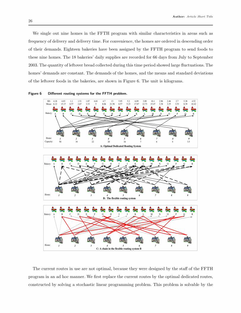
We single out nine homes in the FFTH program with similar characteristics in areas such as

frequency of delivery and delivery time. For convenience, the homes are ordered in descending order

of their demands. Eighteen bakeries have been assigned by the FFTH program to send foods to

these nine homes. The 18 bakeries’ daily supplies are recorded for 66 days from July to September

2003. The quantity of leftover bread collected during this time period showed large fluctuations. The

homes’ demands are constant. The demands of the homes, and the means and standard deviations

of the leftover foods in the bakeries, are shown in Figure 6. The unit is kilograms.

Figure 6 Different routing systems for the FFTH problem.

6.12 15.17 0.57 2.67 3.33 5 8.06 21.58 8.57 5.23 17.87 12.73 15.47 3.38 3.35 3.53 8.39 10.42

50 34 22 20 16 7 6 4 3.5Capacity:

Mean:

4.18 4.03 1.1 1.51 1.87 6.81 4.7 13 5.95 5.2 6.09 3.89 10.1 2.96 2.46 2.7 5.38 4.52SD:

A B C D E F G H I J K L M N O P Q R

1 2 3 4 5 6 7 8 9

Bakery:

Home:

A: Optimal Dedicated Routing System


1 2 3 4 5 6 7 8 9

Bakery:

Home:

B: The flexible routing system


1 2 3 4 5 6 7 8 9

Bakery:

Home:

C: A chain in the flexible routing system B

The current routes in use are not optimal, because they were designed by the staff of the FFTH

program in an ad hoc manner. We first replace the current routes by the optimal dedicated routes,

constructed by solving a stochastic linear programming problem. This problem is solvable by the


27

traditional method, because we assume that the bread from each bakery goes to only one home

(i.e., it has a dedicated route). There is thus no recourse in this stochastic programming problem.

We omit the details here.

We use the performance of the optimal dedicated routing system as a benchmark to assess the

performance of the flexible system designed using our heuristic.

Figure 6-B shows the new flexible routing system obtained by our heuristic. The newly added

arcs help form many long chains in this new flexible system. A long chain that visits nine homes

and nine bakeries is shown in Figure 6-C for illustration. Among the 18 arcs in the chain, 11 are

newly added by our heuristic.

We conduct a simulation analysis to evaluate this flexible system. We assume that the supply

from each bakery is statistically independent, and randomly selected from its historical values.

Daily supplies over 100 days are simulated. We use the expected daily excess as a measure to

evaluate this system.

Figure 7 Average Daily Excess.

Average Daily Oversupply (KG)

2.432 2.809

15.4065

0

2

4

6

8

10

12

14

16

18

Full Flexibility Expander Optimal Dedicated

Overs

up

ply

(K

G)

Figure 7 shows the average daily excess in the full flexibility system, the heuristic flexibility

system, and the optimal dedicated system. By adding 18 arcs to the optimal dedicated system,

the average daily excess decreases significantly from 15.407 kilograms to 2.809 kilograms. It is only

20% of the optimal dedicated system’s excess. Moreover, it is only 0.377 kilograms greater than

the excess of the fully flexible system. On average, the food saving through the flexible routing

system each day (148.64 kg 4) is 99.7% of that through the full flexibility system (149.02 kg 5). This

result not only suggests that our heuristic works well in practice, but also strongly supports the

4 The average daily food savings from the heuristic flexibility system = the average daily leftover food - the averagedaily oversupply of the heuristic = 151.45 - 2.809kg = 148.64 kg.

5 The average daily food savings = 151.45 - 2.432kg = 149.02kg


28

proposition that a flexible delivery system can have a tremendous impact by reducing the amount

of wastage in the program.

6. Conclusions

In this paper, we examine how a flexible process structure might be designed to allow the production

system to better cope with fluctuating supply and demand, and to match supply with demand

in a more effective manner. We argue that good flexible process structures are essentially highly

connected graphs, and use the concept of graph expansion (a measure of graph connectivity) to

achieve various insights into this design problem.

A number of design guidelines are well known in the literature. Principles such as “a long chain

performs better than many short chains,” and that one should “try to equalize the number of plants

(resp. products), measured in total units of capacity (resp. mean demand), which each product

(resp. plant ) in the chain is directly connected to,” can now be interpreted from this new angle

as a development of different ways in which the underlying network can achieve a good expansion

ratio. The same principle extends to other new design guidelines - trying to equalize the number

of plants (measured in total number of units) assigned to each pair (or even triplet) of products,

or vice versa, can also help the decision maker to arrive at a good process structure.

We analyze the worst-case performance of the flexible design problem under a more general

setting, which encompasses a large class of objective functions. We show that whenever demand and

supply are balanced and symmetrical, the graph expander structure (a highly connected but sparse

graph) is within ǫ optimality of the fully flexible system, for all demand scenarios, although it uses

a far smaller number of links. Furthermore, the same graph expander structure works uniformly

well for all objective functions in this class.

Based on this insight, we develop a simple and easy-to-implement heuristic to design flexible

process structure. Numerical results show that this heuristic performs well for a variety of numerical

examples previously studied in the literature. We also use this idea on a set of real data obtained

from a bread delivery system in Singapore, with the goal of minimizing the excess amounts of

bread brought to each location.

Acknowledgments

We would like to thank Henry and Christine from FFTH for the initial discussion on the issues confronting

the program, and Mr. Lee Keng Leong for sharing with us his thoughts on the subject. We would also like

to thank Prof. Sunil Chopra for suggesting that we compare the structures obtained from graph expansion

with what is available in the literature. Thanks also to Prof. Candy Yano who suggested that we look at

more general objective functions for this class of problems.


29

References

Aksin, O. Z., F. Karaesmen. 2007. Characterizing the performance of process flexibility structures. Operations

Research Letters 35(4) 477–484.

Asratian, A., T. Denley, R. Haggkvist. 1998. Bipartite graphs and their applications . Cambridge University

Press.

Bassalygo, L. A., M. S. Pinsker. 1973. Complexity of an optimum non-blocking switching network with

reconnections. Problemy Informatsii (English Translation in Problems of Information Transmission)

9 84–87.

Benjafaar, S. 2002. Modeling and analysis of congestion in the design of facility layouts. Management Science

48(5) 679–704.

Bish, E., A. Muriel, S. Biller. 2005. Managing flexible capacity in a make-to-order environment. Management

Science 51 167–180.

Chou, M. C., G. Chua, C. P. Teo, H. Zheng. 2007. Design for process flexibility: efficiency of the long chain

and sparse structure. To appear in Operations Research.

de Farias, D. P., B. Van Roy. 2004. On constraint sampling in the linear programming approach to approx-

imate dynamic programming. Math. Oper. Res. 29(3) 462–478.

Fiedler, M. 1973. Algebraic connectivity of graphs. Czechoslovak Mathematics Jornal 23 298–305.

Friedman, J. 2003. A proof of alon’s second eigenvalue conjecture. In STOC 03 To Appear.

Ghosh, Arpita, Stephen Boyd. 2006. Growing well-connected graphs. Working Paper .

Graves, S. C., B. T. Tomlin. 2003. Process flexibility in supply chain. Management Science 49(7) 907–919.

Gurumurthi, S., S. Benjaafar. 2004. Modeling and analysis of flexible queueing systems. Naval Research

Logistics 51 755–782.

Hopp, W. J., E. Tekin, M. P. Van Oyen. 2004. Benefits of skill chaining in production lines with cross-trained

workers. Management Science 50(1) 83–98.

Iravani, S. M., M. P. Van Oyen, K. T. Sims. 2005. Structural flexibility: A new perspective on the design of

manufacturing and service operations. Management Science 51(2) 151–166.

Jack, E. P, A. S Raturi. 2003. Measuring and comparing volume flexibility in the capital goods industry.

Production and Operations Management 12(4) 480.

Jordan, W. C., S. C. Graves. 1995. Principles on the benefits of manufacturing process fexibility. Management

Science 41(4) 577–594.

Pinsker, M. 1973. On the complexity of a concentrator. In 7th International Teletraffic Conference. Stock-

holm, 318/1–318/4.

Reingold, O., S. Vadhan, A. Wigderson. 2002. Entropy waves, the zig-zag graph product, and new constant-

degree expanders and extractors. Ann. of Math. 155 157–187.


30

Sarnak, P. 2004. What is an expander? Notices of the AMS 51(7) 762–763.

Sethi, A. K., S. P. Sethi. 1990. Flexibilityin manufacturing: a survey. The Interna-tional Journal of Flexible

ManufacturingSystems 2 289–328.

Shi, D., R. L. Daniels. 2003. A survey of manufacturing flexibility: Implications for e-business. IBM Systems

Journal 42(3) 414–427.

Tanner, R. M. 1981. A recursive approach to low complexity codes. IEEE Trans. Inform. Theory 27 533–547.

Appendix

Proof of Theorem 2:

Consider the following probabilistic method to generate a flexibility structure: For each node in A, pick ∆

neighbors in B randomly. For each set U with |U |= z ≤ αn, the probability that all neighbors are contained

in a set V with |V | = λz is given by (λz/n)z∆. There are

n

z

and

n

λz

ways to choose U and V

respectively. Hence the probability that there exist such sets U and V is at most

gz =

n

z

n

λz

(λz/n)z∆ ≤ (ne

z)z(

ne

λz)λz(λz/n)z∆,

using the inequality

n

k

≤ (ne/k)k. Re-arranging the terms, and using the fact that z ≤ αn, we have

gz ≤

[

n1+λ−∆e1+λλ∆−λz∆−λ−1

]z

≤

[

e1+λλ(αλ)∆−λ−1

]z

.

By picking ∆ at least as large as the lowerbound as shown in the theorem, we can ensure that gz ≤ (1/2)z.

Note that αλ < 1 is crucial for this to hold. Hence the probability that there exists some set U with |U | ≤ αn,

with |N(U)| ≤ λ|U |, is at most∑αn

z=1 gz < 1. Hence (α,λ,∆)-expander exists.

Proof of Theorem 4:

Consider any given D = Di. The KKT conditions are the same as the conditions for the symmetrical

problem considered in Theorem 1, except that (3) needs to be adjusted slightly as the following:

U ′j

(

∑

l∈A

x∗lj

)

−u∗i + v∗

ij = 0 ∀ (i, j)∈F (14)

Let S(D)∆=

(i, j) : x∗i,j > 0

and S(D)∆=

(i, j) : x∗i,j = 0

. S(D) can be easily written as a union of

connected components Sk , k = 1, . . . , h. The KKT conditions ensure that, for any k = 1, . . . , h,

U ′j

(

∑

i:i∈A

x∗i,j

)

= βk, ∀j ∈B∩Sk,

where βk is a constant. WLOG we can assume that β1 < β2 < . . . < βh, since we can otherwise combine

components with identical βk together.


31

Let S0∆= ∪Si : βi < K, T

∆=A∩S0, and S0

∆= S(D)/S0, T

∆=A∩ S0.

In the structure F , we note that

Γ(T ) = Γ(A∩S0)⊆B∩S0. (15)

This is because if (15) does not hold, then there exists an edge (i, j) ∈F with i∈A∩Sk, for some Sk ⊆ S0,

but j /∈ B∩S0, which implies that either

• j ∈ B∩Sm, for some Sm ⊆ S0 = S(D)/S0, or

• j has a flow of zero; that is, x∗i,j = 0 for all i∈A.

But in the first case, the KKT condition (3) ensures that

U ′j(∑

l∈A

x∗lj)− u∗

i ≤ 0,

i.e., βm ≤ u∗i = βk < K, which is a contradiction. In the second case, since for all j ∈ B, Uj(·) is a concave

function and Uj(x) = Kx when 0 ≤ x ≤ Cj , we can always reallocate one unit of the demand for i to plant

j without decreasing the value of ZF(D). Therefore, WLOG, we can exclude the possibility of the second

case. From the above arguments, we know that (15) must hold.

On the other hand, it is easy to see that

B∩S0 ⊆Γ(T ). (16)

Hence, we have

Γ(T ) = B∩S0. (17)

Also note that

x∗ij = 0, ∀i∈ T and j ∈ Γ(T ). (18)

(18) holds because otherwise, there must exists an arc (i, j) ∈ F with i ∈ T , j ∈ Γ(T ), and x∗ij > 0. In that

case, the KKT conditions ensure that U ′j(∑

l∈Ax∗

lj) = ui ≥ K, which contradicts that U ′j(∑

l∈Ax∗

lj) < K for

all j ∈ Γ(T ).

From (17) and (18), we must have

∑

i∈A∩S0

(

∑

j∈B

x∗ij

)

=∑

j∈B∩S0

(

∑

i∈A

x∗ij

)

. (19)

Similarly, we can see that∑

i∈A∩S0

(

∑

j∈B

x∗ij

)

=∑

j∈B∩S0

(

∑

i∈A

x∗ij

)

. (20)

We now consider three cases:

Case (a): If T = ∅, then S0 = ∅ and S0 = S(D). Note that for all j ∈B, either

• j ∈ S(D)∩B, or

• j ∈ S(D)∩B.


32

In the first case, since S0 = S(D), we have j ∈ S0 ∩ B. Therefore, U ′j(∑

l∈A x∗lj) ≥ K since βk ≥ K for all

Sk ⊆ S0. Also note that Uj(x) is a concave function with U ′j(x) < K when x > Cj, thus we have

∑

l∈Ax∗

lj ≤Cj .

In the second case, from the definition of S(D), it is obvious that∑

l∈Ax∗

lj = 0 ≤ Cj . Hence, combining

the above two cases, we conclude that∑

l∈Ax∗

lj ≤ Cj for all j ∈ B. That is, all plants operate under their

capacity level.

Case(b): If T is a small subset, then from (17), (20), the definition of Ψ-expander (Definition 5), and the

definition of a small subset (Definition 6), we must have

∑

j∈Γ(T )

(

∑

i∈A

x∗ij

)

=∑

i∈T

Di ≤∑

i∈T

λUi µi ≤

∑

j∈Γ(T )

Cj .

However, since

• Uj(x) is a concave function with U ′j(x) = K when 0≤ x≤Cj , and

• U ′j(∑

i∈Ax∗

ij) < K for all j ∈ Γ(T ),

we must have∑

i∈Ax∗

ij > Cj for all j ∈ Γ(T ), and hence,∑

j∈Γ(T )

(∑

i∈Ax∗

ij

)

>∑

j∈Γ(T ) Cj , which is a

contradiction. Thus T cannot be a small subset.

Case(c): If T is a non-small subset, then from the definition of a non-small subset (Definition 6), we have∑

i∈TλU

i µi > Ψ∑

j∈BCj −

∑

i/∈TλL

i µi.

• If∑

i∈TDi ≤

∑

j∈Γ(T ) Cj, then using some of the arguments in Case(b), we can show that∑

j∈Γ(T )

(∑

i∈Ax∗

ij

)

≤∑

j∈Γ(T ) Cj and∑

j∈Γ(T )

(∑

i∈Ax∗

ij

)

>∑

j∈Γ(T ) Cj , which is a contradiction.

• If∑

i∈T Di >∑

j∈Γ(T ) Cj , then for all j ∈ Γ(T ),∑

i∈T x∗ij ≥ Cj since Uj(·) is a non-decreasing concave

function with Uj(x) = Kx for 0 ≤ x ≤ Cj and U ′j(x) < K for x > Cj. Since

∑

i∈Ax∗

ij ≥∑

i∈Tx∗

ij , we have∑

i∈Ax∗

ij ≥Cj , ∀j ∈ Γ(T ), thus∑

j∈Γ(T ) Cj is fully utilized.

Note that∑

i∈A

x∗ij ≤Cj, ∀j ∈B∩ S0,

because U ′j

(∑

i∈Ax∗

ij

)

≥K for all j ∈B∩ S0. Also note that, by Equation (19), we have

∑

i∈T

λLi µi ≤

∑

i∈T

(

∑

j∈B

x∗ij

)

=∑

j∈B∩S0

(

∑

i∈A

x∗ij

)

≤∑

j∈B∩S0

Cj .

Therefore, all the plants in B ∩ S0 operate within its preconfigured capacity Cj , with at least∑

i∈TλL

i µi

capacity utilized. According to the definition of Ψ-expander, we know that

∑

j∈Γ(T )

Cj +∑

i∈T

λLi µi ≥Ψ

∑

j∈B

Cj ,

hence we have at least Ψ proportion of the preconfigured capacity being utilized.

process flexibility revisited: the graph expander and its applications

Documents