irrigander 4/8 expander

87

CHAPTER 5

MODELS FOR NONSTATIONARY TIME SERIES

Any time series without a constant mean over time is nonstationary. Models of the form

Yt = μt + Xt

where μt is a nonconstant mean function and Xt is a zero-mean, stationary series, wereconsidered in Chapter 3. As stated there, such models are reasonable only if there aregood reasons for believing that the deterministic trend is appropriate “forever.” That is,just because a segment of the series looks like it is increasing (or decreasing) approxi-mately linearly, do we believe that the linearity is intrinsic to the process and will persistin the future? Frequently in applications, particularly in business and economics, wecannot legitimately assume a deterministic trend. Recall the random walk displayed inExhibit 2.1, on page 14. The time series appears to have a strong upward trend thatmight be linear in time. However, also recall that the random walk process has a con-stant, zero mean and contains no deterministic trend at all.

As an example consider the monthly price of a barrel of crude oil from January1986 through January 2006. Exhibit 5.1 displays the time series plot. The series displaysconsiderable variation, especially since 2001, and a stationary model does not seem tobe reasonable. We will discover in Chapters 6, 7, and 8 that no deterministic trendmodel works well for this series but one of the nonstationary models that have beendescribed as containing stochastic trends does seem reasonable. This chapter discussessuch models. Fortunately, as we shall see, many stochastic trends can be modeled withrelatively few parameters.

88 Models for Nonstationary Time Series

Exhibit 5.1 Monthly Price of Oil: January 1986–January 2006

> win.graph(width=4.875,height=3,pointsize=8)> data(oil.price)> plot(oil.price, ylab='Price per Barrel',type='l')

5.1 Stationarity Through Differencing

Consider again the AR(1) model(5.1.1)

We have seen that assuming et is a true “innovation” (that is, et is uncorrelated withYt − 1, Yt − 2,…), we must have |φ| < 1. What can we say about solutions to Equation(5.1.1) if |φ| ≥ 1? Consider in particular the equation

(5.1.2)

Iterating into the past as we have done before yields

(5.1.3)

We see that the influence of distant past values of Yt and et does not die out—indeed,the weights applied to Y0 and e1 grow exponentially large. In Exhibit 5.2, we show thevalues for a very short simulation of such a series. Here the white noise sequence wasgenerated as standard normal variables and we used Y0 = 0 as an initial condition.

Exhibit 5.2 Simulation of the Explosive “AR(1) Model”

t 1 2 3 4 5 6 7 8

et 0.63 −1.25 1.80 1.51 1.56 0.62 0.64 −0.98

Yt 0.63 0.64 3.72 12.67 39.57 119.33 358.63 1074.91

Time

Pric

e pe

r B

arre

l

1990 1995 2000 2005

1020

3040

5060

Yt φYt 1– et+=

Yt 3Yt 1– et+=

Yt et 3et 1– 32et 2–… 3t 1– e1 3tY0+ + + + +=

Yt 3Yt 1– et+=

5.1 Stationarity Through Differencing 89

Exhibit 5.3 shows the time series plot of this explosive AR(1) simulation.

Exhibit 5.3 An Explosive “AR(1)” Series

> data(explode.s)> plot(explode.s,ylab=expression(Y[t]),type='o')

The explosive behavior of such a model is also reflected in the model’s varianceand covariance functions. These are easily found to be

(5.1.4)

and

(5.1.5)

respectively. Notice that we have

The same general exponential growth or explosive behavior will occur for any φsuch that |φ| > 1. A more reasonable type of nonstationarity obtains when φ = 1. If φ = 1,the AR(1) model equation is

(5.1.6)

This is the relationship satisfied by the random walk process of Chapter 2 (Equation(2.2.9) on page 12). Alternatively, we can rewrite this as

(5.1.7)

● ● ● ●●

●

●

●

Time

Yt

1 2 3 4 5 6 7 8

020

040

060

080

010

00

Var Yt( ) 18--- 9 t 1–( )σe

2=

Cov Yt Yt k–,( ) 3k

8----- 9 t k– 1–( )σe

2=

Corr Yt Yt k–,( ) 3k 9t k– 1–

9t 1–-------------------- 1≈= for large t and moderate k

Yt Yt et+=

∇Yt et=


where is the first difference of Yt. The random walk then is easilyextended to a more general model whose first difference is some stationary pro-cess—not just white noise.

Several somewhat different sets of assumptions can lead to models whose first dif-ference is a stationary process. Suppose

(5.1.8)

where Mt is a series that is changing only slowly over time. Here Mt could be eitherdeterministic or stochastic. If we assume that Mt is approximately constant over everytwo consecutive time points, we might estimate (predict) Mt at t by choosing β0 so that

is minimized. This clearly leads to

and the “detrended” series at time t is then

This is a constant multiple of the first difference, ∇Yt.†

A second set of assumptions might be that Mt in Equation (5.1.8) is stochastic andchanges slowly over time governed by a random walk model. Suppose, for example, that

(5.1.9)

where {et} and {εt} are independent white noise series. Then

which would have the autocorrelation function of an MA(1) series with

(5.1.10)

In either of these situations, we are led to the study of ∇Yt as a stationary process.Returning to the oil price time series, Exhibit 5.4 displays the time series plot of the

differences of logarithms of that series.‡ The differenced series looks much more sta-tionary when compared with the original time series shown in Exhibit 5.1, on page 88.

† A more complete labeling of this difference would be that it is a first difference at lag 1.‡ In Section 5.4 on page 98 we will see why logarithms are often a convenient transforma-

tion.

∇Yt Yt Yt 1––=

Yt Mt Xt+=

Yt j– β0 t,–( )2

j 0=

1∑

M̂t12--- Yt Yt 1–+( )=

Yt M̂t– Yt12--- Yt Yt 1–+( )–

12--- Yt Yt 1––( ) 1

2---∇Yt= = =

Yt Mt et+= with Mt Mt 1– εt+=

Yt∇ Mt∇ et∇+=

εt et et 1––+=

ρ1 1 2 σε2 σe

2⁄( )+[ ]⁄{ }–=

5.1 Stationarity Through Differencing 91

(We will also see later that there are outliers in this series that need to be considered toproduce an adequate model.)

Exhibit 5.4 The Difference Series of the Logs of the Oil Price Time

> plot(diff(log(oil.price)),ylab='Change in Log(Price)',type='l')

We can also make assumptions that lead to stationary second-difference models.Again we assume that Equation (5.1.8) on page 90, holds, but now assume that Mt is lin-ear in time over three consecutive time points. We can now estimate (predict) Mt at themiddle time point t by choosing and to minimize

The solution yields

and thus the detrended series is

a constant multiple of the centered second difference of Yt. Notice that we have differ-enced twice, but both differences are at lag 1.

Alternatively, we might assume that

Time

Cha

nge

in L

og(P

rice)

1990 1995 2000 2005

−0.

4−

0.2

0.0

0.2

0.4

β0 t, β1 t,

Yt j– β0 t, jβ1 t,+( )–( )2

j 1–=

1

∑

M̂t13--- Yt 1+ Yt Yt 1–+ +( )=

Yt M̂t– Yt

Yt 1+ Yt Yt 1–+ +

3------------------------------------------⎝ ⎠

⎛ ⎞–=

13---–⎝ ⎠

⎛ ⎞ Yt 1+ 2Yt– Yt 1–+( )=

13---–⎝ ⎠

⎛ ⎞ Yt 1+∇( )∇=

13---–⎝ ⎠

⎛ ⎞ ∇2 Yt 1+( )=


(5.1.11)

with {et} and {εt} independent white noise time series. Here the stochastic trend Mt issuch that its “rate of change,” ∇Mt, is changing slowly over time. Then

and

which has the autocorrelation function of an MA(2) process. The important point is thatthe second difference of the nonstationary process {Yt} is stationary. This leads us to thegeneral definition of the important integrated autoregressive moving average time seriesmodels.

5.2 ARIMA Models

A time series {Yt} is said to follow an integrated autoregressive moving averagemodel if the dth difference Wt = ∇dYt is a stationary ARMA process. If {Wt} follows anARMA(p,q) model, we say that {Yt} is an ARIMA(p,d,q) process. Fortunately, forpractical purposes, we can usually take d = 1 or at most 2.

Consider then an ARIMA(p,1,q) process. With Wt = Yt − Yt − 1, we have

(5.2.1)

or, in terms of the observed series,

which we may rewrite as

(5.2.2)

We call this the difference equation form of the model. Notice that it appears to be anARMA(p + 1,q) process. However, the characteristic polynomial satisfies

Yt Mt et,+= where Mt Mt 1– Wt+= and Wt Wt 1– εt+=

Yt∇ Mt∇ et∇+ Wt et∇+= =

∇2Yt Wt∇ ∇2et+=

εt et et 1––( ) et 1– et 2––( )–+=

εt et 2et 1–– et 2–+ +=

Wt φ1Wt 1– φ2Wt 2–… φpWt p– et+ + + += θ1et 1– θ2et 2––

…– θqet q–––

Yt Yt 1–– φ1 Yt 1– Yt 2––( ) φ2 Yt 2– Yt 3––( ) … φp Yt p– Yt p– 1––( )+ + +=

et+ θ1et 1– θ2et 2–– …– θqet q–––

Yt 1 φ1+( )Yt 1– φ2 φ1–( )Yt 2– φ3 φ2–( )Yt 3–…+ + +=

φp φp 1––( )+ Yt p– φpYt p– 1–– et θ1et 1– θ2et 2–– …– θqet q–––+

1 1 φ1+( )x– φ2 φ1–( )x2– φ3 φ2–( )x3– …– φp φp 1––( )xp– φpxp 1++

1 φ1x– φ2x2– …– φpxp–( ) 1 x–( )=

5.2 ARIMA Models 93

which can be easily checked. This factorization clearly shows the root at x = 1, whichimplies nonstationarity. The remaining roots, however, are the roots of the characteristicpolynomial of the stationary process ∇Yt.

Explicit representations of the observed series in terms of either Wt or the whitenoise series underlying Wt are more difficult than in the stationary case. Since nonsta-tionary processes are not in statistical equilibrium, we cannot assume that they go infi-nitely into the past or that they start at . However, we can and shall assume thatthey start at some time point , say, where is earlier than time t = 1, at whichpoint we first observed the series. For convenience, we take Yt = 0 for t < −m. The differ-ence equation Yt − Yt − 1 = Wt can be solved by summing both sides from to t =t to get the representation

(5.2.3)

for the ARIMA(p,1,q) process.The ARIMA(p,2,q) process can be dealt with similarly by summing twice to get the

representations

(5.2.4)

These representations have limited use but can be used to investigate the covarianceproperties of ARIMA models and also to express Yt in terms of the white noise series{et}. We defer the calculations until we evaluate specific cases.

If the process contains no autoregressive terms, we call it an integrated movingaverage and abbreviate the name to IMA(d,q). If no moving average terms are present,we denote the model as ARI(p,d). We first consider in detail the important IMA(1,1)model.

The IMA(1,1) Model

The simple IMA(1,1) model satisfactorily represents numerous time series, especiallythose arising in economics and business. In difference equation form, the model is

(5.2.5)

To write Yt explicitly as a function of present and past noise values, we use Equation(5.2.3) and the fact that Wt = et − θet − 1 in this case. After a little rearrangement, we canwrite

(5.2.6)

Notice that in contrast to our stationary ARMA models, the weights on the white noiseterms do not die out as we go into the past. Since we are assuming that −m < 1 and 0 < t,we may usefully think of Yt as mostly an equally weighted accumulation of a large num-ber of white noise values.

t ∞–=t m–= m–

t m–=

Yt Wjj m–=

t

∑=

Yt Wii m–=

j

∑j m–=

t

∑=

j 1+( )Wt j–j 0=

t m+

∑=

Yt Yt 1– et θet 1––+=

Yt et 1 θ–( )et 1– 1 θ–( )et 2–… 1 θ–( )e m– θe m– 1––+ + + +=


From Equation (5.2.6), we can easily derive variances and correlations. We have

(5.2.7)

and

(5.2.8)

We see that as t increases, increases and could be quite large. Also, the correla-tion between Yt and Yt − k will be strongly positive for many lags k = 1, 2, … .

The IMA(2,2) Model

The assumptions of Equation (5.1.11) led to an IMA(2,2) model. In difference equationform, we have

or(5.2.9)

The representation of Equation (5.2.4) may be used to express Yt in terms of et, et − 1,….After some tedious algebra, we find that

(5.2.10)

where ψj = 1 + θ2 + (1 − θ1 − θ2) j for j = 1, 2, 3,…, t + m. Once more we see that theψ-weights do not die out but form a linear function of j.

Again, variances and correlations for Yt can be obtained from the representationgiven in Equation (5.2.10), but the calculations are tedious. We shall simply note that thevariance of Yt increases rapidly with t and again is nearly 1 for all mod-erate k.

The results of a simulation of an IMA(2,2) process are displayed in Exhibit 5.5.Notice the smooth change in the process values (and the unimportance of the zero-meanfunction). The increasing variance and the strong, positive neighboring correlationsdominate the appearance of the time series plot.

Var Yt( ) 1 θ2 1 θ–( )2 t m+( )+ +[ ]σe2=

Corr Yt Yt k–,( ) 1 θ– θ2 1 θ–( )2 t m k–+( )+ +

Var Yt( )Var Yt k–( )[ ]1 2/----------------------------------------------------------------------------=

t m k–+t m+

---------------------≈

1≈ for large m and moderate k

Var Yt( )

∇2Yt et θ1et 1–– θ2et 2––=

Yt 2Yt 1– Yt 2–– et θ1et 1–– θ2et 2––+=

Yt et ψjet j–j 1=

t m+

∑ t m 1+ +( )θ1 t m+( )θ2+[ ]e m– 1––+=

t m 1+ +( )θ2e m– 2––

Corr Yt Yt k–,( )

5.2 ARIMA Models 95

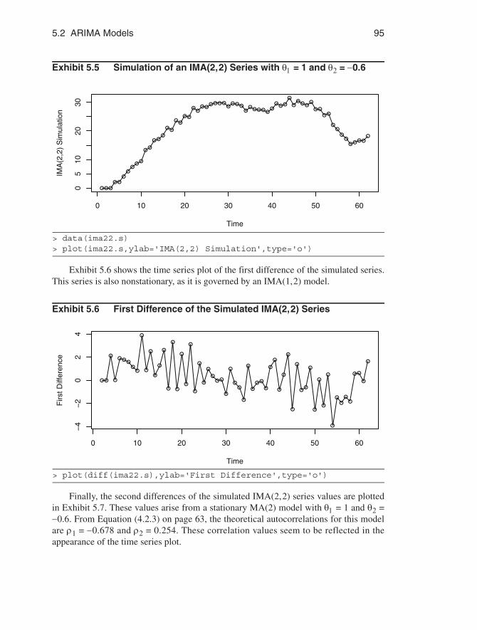
Exhibit 5.5 Simulation of an IMA(2,2) Series with θ1 = 1 and θ2 = −0.6

> data(ima22.s)> plot(ima22.s,ylab='IMA(2,2) Simulation',type='o')

Exhibit 5.6 shows the time series plot of the first difference of the simulated series.This series is also nonstationary, as it is governed by an IMA(1,2) model.

Exhibit 5.6 First Difference of the Simulated IMA(2,2) Series

> plot(diff(ima22.s),ylab='First Difference',type='o')

Finally, the second differences of the simulated IMA(2,2) series values are plottedin Exhibit 5.7. These values arise from a stationary MA(2) model with θ1 = 1 and θ2 =−0.6. From Equation (4.2.3) on page 63, the theoretical autocorrelations for this modelare ρ1 = −0.678 and ρ2 = 0.254. These correlation values seem to be reflected in theappearance of the time series plot.

●●●

●●●

●●

●●

●●

●●●

●●

●●

●●

●●

●●●●●●

●●●●

●●●●●●

●●

●●

●

●●

●●●

●●

●●

●●

●●

●●●●●

Time

IMA

(2,2

) S

imul

atio

n

0 10 20 30 40 50 60

05

1020

30

● ●

●

●

● ● ●●

●

●

●

●

●

●

●

●

●

●

●

●

●

●

●

●

●

●● ●

●

●

●●

●

●

●

● ●

●

●

●

●

●

●

●

●

●●

●

●

●

●

●

●

●●

●●

● ●

●

●

Time

Firs

t Diff

eren

ce

0 10 20 30 40 50 60

−4

−2

02

4


Exhibit 5.7 Second Difference of the Simulated IMA(2,2) Series

> plot(diff(ima22.s,difference=2),ylab='Differenced Twice',type='o')

The ARI(1,1) Model

The ARI(1,1) process will satisfy

(5.2.11)

or(5.2.12)

where |φ| < 1.†

To find the ψ-weights in this case, we shall use a technique that will generalize toarbitrary ARIMA models. It can be shown that the ψ-weights can be obtained by equat-ing like powers of x in the identity:

(5.2.13)

In our case, this relationship reduces to

or

Equating like powers of x on both sides, we obtain

† Notice that this looks like a special AR(2) model. However, one of the roots of the corre-sponding AR(2) characteristic polynomial is 1, and this is not allowed in stationary AR(2)models.

●

●

●

●

● ●● ●

●

●

●

●

●●

●

●

●

●

●

●

●

●

●

●

● ●●

●

●

●

●

●

●

●

●●

●

●

●

●

●●

●

●

●

●

●

●

●

●

●

●

●

●

●

●

●

●

●

●

Time

Diff

eren

ced

Tw

ice

10 20 30 40 50 60

−4

−2

02

4

Yt Yt 1–– φ Yt 1– Yt 2––( ) et+=

Yt 1 φ+( )Yt 1– φYt 2–– et+=

1 φ1x– φ2x2– …– φpxp–( ) 1 x–( )d 1 ψ1x ψ2x2 ψ3x3 …+ + + +( )

1 θ1x– θ2x2– θ3x3– …– θqxq–( )=

1 φx–( ) 1 x–( ) 1 ψ1x ψ2x2 ψ3x3 …+ + + +( ) 1=

1 1 φ+( )x– φx2+[ ] 1 ψ1x ψ2x2 ψ3x3 …+ + + +( ) 1=

5.3 Constant Terms in ARIMA Models 97

and, in general,(5.2.14)

with ψo = 1 and ψ1 = 1 + φ. This recursion with starting values allows us to compute asmany ψ-weights as necessary. It can also be shown that in this case an explicit solutionto the recursion is given as

(5.2.15)

(It is easy, for example, to show that this expression satisfies Equation (5.2.14).

5.3 Constant Terms in ARIMA Models

For an ARIMA(p,d,q) model, ∇dYt = Wt is a stationary ARMA(p,q) process. Our stan-dard assumption is that stationary models have a zero mean; that is, we are actuallyworking with deviations from the constant mean. A nonzero constant mean, μ, in a sta-tionary ARMA model {Wt} can be accommodated in either of two ways. We canassume that

Alternatively, we can introduce a constant term θ0 into the model as follows:

Taking expected values on both sides of the latter expression, we find that

so that

(5.3.16)

or, conversely, that

(5.3.17)

Since the alternative representations are equivalent, we shall use whichever parameter-ization is convenient.

1 φ+( )– ψ1+ 0=

φ 1 φ+( )ψ1 ψ2+– 0=

ψk 1 φ+( )ψk 1– φψk 2––= for k 2≥

ψk1 φk 1+–

1 φ–---------------------- for k 1≥=

Wt μ– φ1 Wt 1– μ–( ) φ2 Wt 2– μ–( ) … φp Wt p– μ–( )+ + +=

et+ θ1et 1– θ2et 2–– …– θqet q–––

Wt θ0 φ1Wt 1– φ2Wt 2–… φpWt p–+ + ++=

et θ1et 1– θ2et 2–– …– θqet q–––+

μ θ0 φ1 φ2… φp+ + +( )μ+=

μθ0

1 φ1 φ2– …– φp––--------------------------------------------------=

θ0 μ 1 φ1 φ2– …– φp––( )=


What will be the effect of a nonzero mean for Wt on the undifferenced series Yt?Consider the IMA(1,1) case with a constant term. We have

or

Either by substituting into Equation (5.2.3) on page 93 or by iterating into the past, wefind that

(5.3.18)

Comparing this with Equation (5.2.6), we see that we have an added linear deterministictime trend (t + m + 1)θ0 with slope θ0.

An equivalent representation of the process would then be

where is an IMA(1,1) series with E = 0 and E = β1. For a general ARIMA(p,d,q) model where E ≠ 0, it can be argued that Yt =

, where μt is a deterministic polynomial of degree d and is ARIMA(p,d,q)with E = 0. With d = 2 and θ0 ≠ 0, a quadratic trend would be implied.

5.4 Other Transformations

We have seen how differencing can be a useful transformation for achieving stationarity.However, the logarithm transformation is also a useful method in certain circumstances.We frequently encounter series where increased dispersion seems to be associated withhigher levels of the series—the higher the level of the series, the more variation there isaround that level and conversely.

Specifically, suppose that Yt > 0 for all t and that

(5.4.1)

Then

(5.4.2)

These results follow from taking expected values and variances of both sides of the(Taylor) expansion

In words, if the standard deviation of the series is proportional to the level of the series,then transforming to logarithms will produce a series with approximately constant vari-ance over time. Also, if the level of the series is changing roughly exponentially, the

Yt Yt 1– θ0 et θet 1––+ +=

Wt θ0 et θet 1––+=

Yt et 1 θ–( )et 1– 1 θ–( )et 2–… 1 θ–( )e m– θe m– 1––+ + + +=

t m 1+ +( )θ0+

Yt Yt' β0 β1t+ +=

Yt' Yt'∇( ) Yt∇( )∇dYt( )

Yt' μt+ Yt'Yt'

E Yt( ) μt= and Var Yt( ) μtσ=

E Yt( )log[ ] μt( )log≈ and Var Yt( )log( ) σ2≈

Yt( )log μt( )logYt μt–

μt---------------+≈

5.4 Other Transformations 99

log-transformed series will exhibit a linear time trend. Thus, we might then want to takefirst differences. An alternative set of assumptions leading to differences of logged datafollows.

Percentage Changes and Logarithms

Suppose Yt tends to have relatively stable percentage changes from one time period tothe next. Specifically, assume that

where 100Xt is the percentage change (possibly negative) from Yt−1 to Yt. Then

If Xt is restricted to, say, |Xt| < 0.2 (that is, the percentage changes are at most ±20%),then, to a good approximation, log(1+Xt) ≈ Xt. Consequently,

(5.4.3)

will be relatively stable and perhaps well-modeled by a stationary process. Notice thatwe take logs first and then compute first differences—the order does matter. In financialliterature, the differences of the (natural) logarithms are usually called returns.

As an example, consider the time series shown in Exhibit 5.8. This series gives thetotal monthly electricity generated in the United States in millions of kilowatt-hours.The higher values display considerably more variation than the lower values.

Exhibit 5.8 U.S. Electricity Generated by Month

> data(electricity); plot(electricity)

Yt 1 Xt+( )Yt 1–=

Yt( )log Yt 1–( )log–Yt

Yt 1–------------⎝ ⎠

⎛ ⎞log=

1 Xt+( )log=

∇ Yt( )log[ ] Xt≈

Time

Ele

ctric

ity

1975 1980 1985 1990 1995 2000 2005

1500

0025

0000

3500

00


Exhibit 5.9 displays the time series plot of the logarithms of the electricity values.Notice how the amount of variation around the upward trend is now much more uniformacross high and low values of the series.

Exhibit 5.9 Time Series Plot of Logarithms of Electricity Values

> plot(log(electricity),ylab='Log(electricity)')

The differences of the logarithms of the electricity values are displayed in Exhibit5.10. On the basis of this plot, we might well consider a stationary model as appropriate.

Exhibit 5.10 Difference of Logarithms for Electricity Time Series

> plot(diff(log(electricity)), ylab='Difference of Log(electricity)')

Time

Log(

elec

tric

ity)

1975 1980 1985 1990 1995 2000 2005

12.0

12.4

12.8

Time

Diff

eren

ce o

f Log

(ele

ctric

ity)

1975 1980 1985 1990 1995 2000 2005

−0.

2−

0.1

0.0

0.1

5.4 Other Transformations 101

Power Transformations

A flexible family of transformations, the power transformations, was introduced byBox and Cox (1964). For a given value of the parameter λ, the transformation is definedby

(5.4.4)

The term xλ is the important part of the first expression, but subtracting 1 and dividingby λ makes g(x) change smoothly as λ approaches zero. In fact, a calculus argument†

shows that as λ , (xλ − 1)/λ log(x). Notice that λ = ½ produces a square roottransformation useful with Poisson-like data, and λ = −1 corresponds to a reciprocaltransformation.

The power transformation applies only to positive data values. If some of the valuesare negative or zero, a positive constant may be added to all of the values to make themall positive before doing the power transformation. The shift is often determined subjec-tively. For example, for nonnegative catch data in biology, the occurrence of zeros isoften dealt with by adding a constant equal to the smallest positive data value to all ofthe data values. An alternative approach consists of using transformations applicable toany data—positive or not. A drawback of this alternative approach is that interpretationsof such transformations are often less straightforward than the interpretations of thepower transformations. See Yeo and Johnson (2000) and the references containedtherein.

We can consider λ as an additional parameter in the model to be estimated from theobserved data. However, precise estimation of λ is usually not warranted. Evaluation ofa range of transformations based on a grid of λ values, say ±1, ±1/2, ±1/3, ±1/4, and 0,will usually suffice and may have some intuitive meaning.

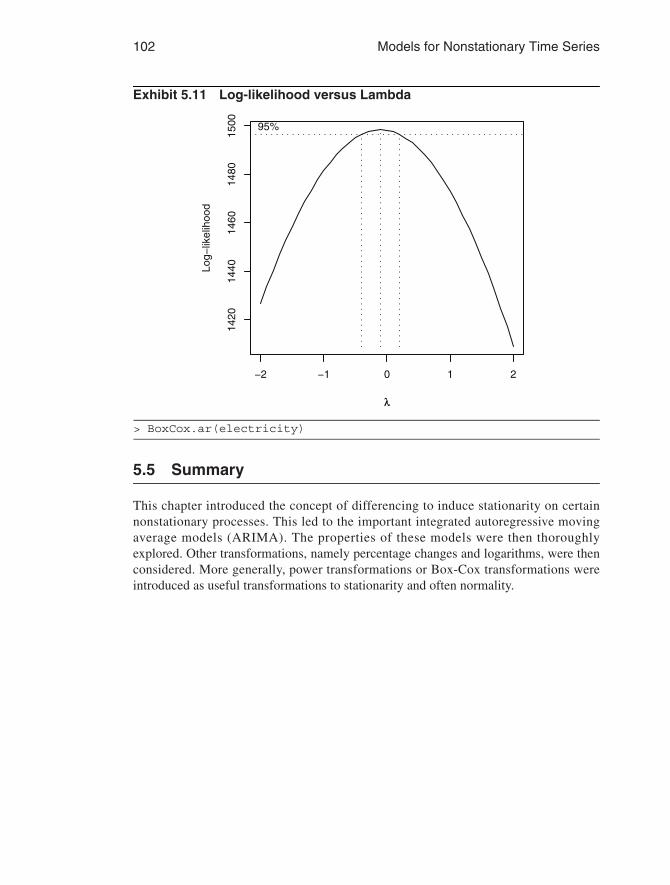
Software allows us to consider a range of lambda values and calculate a log-likeli-hood value for each lambda value based on a normal likelihood function. A plot of thesevalues is shown in Exhibit 5.11 for the electricity data. The 95% confidence interval forλ contains the value of λ = 0 quite near its center and strongly suggests a logarithmictransformation (λ = 0) for these data.

† Exercise (5.17) asks you to verify this.

g x( )xλ 1–

λ-------------- for λ 0≠

xlog for λ 0=⎩⎪⎨⎪⎧

=

0→ →


Exhibit 5.11 Log-likelihood versus Lambda

> BoxCox.ar(electricity)

5.5 Summary

This chapter introduced the concept of differencing to induce stationarity on certainnonstationary processes. This led to the important integrated autoregressive movingaverage models (ARIMA). The properties of these models were then thoroughlyexplored. Other transformations, namely percentage changes and logarithms, were thenconsidered. More generally, power transformations or Box-Cox transformations wereintroduced as useful transformations to stationarity and often normality.

−2 −1 0 1 2

1420

1440

1460

1480

1500

λλ

Log−

likel

ihoo

d

95%

Exercises 103

EXERCISES

5.1 Identify the following as specific ARIMA models. That is, what are p, d, and qand what are the values of the parameters (the φ’s and θ’s)?(a) Yt = Yt − 1 − 0.25Yt − 2 + et − 0.1et − 1.(b) Yt = 2Yt − 1 − Yt−2 + et.(c) Yt = 0.5Yt − 1 − 0.5Yt − 2 + et − 0.5et − 1+ 0.25et − 2.

5.2 For each of the ARIMA models below, give the values for E(∇Yt) and Var(∇Yt).(a) Yt = 3 + Yt − 1 + et − 0.75et − 1.(b) Yt = 10 + 1.25Yt − 1 − 0.25Yt − 2 + et − 0.1et − 1.(c) Yt = 5 + 2Yt − 1 − 1.7Yt − 2 + 0.7Yt − 3 + et − 0.5et − 1+ 0.25et − 2.

5.3 Suppose that {Yt} is generated according to Yt = et + cet − 1+ cet − 2+ cet − 3+ +ce0 for t > 0.(a) Find the mean and covariance functions for {Yt}. Is {Yt} stationary?(b) Find the mean and covariance functions for {∇Yt}. Is {∇Yt} stationary?(c) Identify {Yt} as a specific ARIMA process.

5.4 Suppose that Yt = A + Bt + Xt, where {Xt} is a random walk. First suppose that Aand B are constants.(a) Is {Yt} stationary?(b) Is {∇Yt} stationary?

Now suppose that A and B are random variables that are independent of the random walk {Xt}.

(c) Is {Yt} stationary?(d) Is {∇Yt} stationary?

5.5 Using the simulated white noise values in Exhibit 5.2, on page 88, verify the val-ues shown for the explosive process Yt.

5.6 Consider a stationary process {Yt}. Show that if ρ1 < ½, ∇Yt has a larger variancethan does Yt.

5.7 Consider two models:A: Yt = 0.9Yt − 1 + 0.09Yt − 2 + et.B: Yt = Yt − 1 + et − 0.1et − 1.

(a) Identify each as a specific ARIMA model. That is, what are p, d, and q andwhat are the values of the parameters, φ’s and θ’s?(b) In what ways are the two models different?(c) In what ways are the two models similar? (Compare ψ-weights and

π-weights.)

…


5.8 Consider a nonstationary “AR(1)” process defined as a solution to Equation(5.1.2) on page 88, with |φ| > 1.(a) Derive an equation similar to Equation (5.1.3) on page 88, for this more gen-eral case. Use Y0 = 0 as an initial condition.(b) Derive an equation similar to Equation (5.1.4) on page 89, for this more gen-

eral case.(c) Derive an equation similar to Equation (5.1.5) on page 89, for this more gen-

eral case.(d) Is it true that for any |φ| > 1, for large t and moderate k?

5.9 Verify Equation (5.1.10) on page 90.5.10 Nonstationary ARIMA series can be simulated by first simulating the correspond-

ing stationary ARMA series and then “integrating” it (really partially summingit). Use statistical software to simulate a variety of IMA(1,1) and IMA(2,2) serieswith a variety of parameter values. Note any stochastic “trends” in the simulatedseries.

5.11 The data file winnebago contains monthly unit sales of recreational vehicles(RVs) from Winnebago, Inc., from November 1966 through February 1972.(a) Display and interpret the time series plot for these data.(b) Now take natural logarithms of the monthly sales figures and display the time

series plot of the transformed values. Describe the effect of the logarithms onthe behavior of the series.

(c) Calculate the fractional relative changes, (Yt − Yt − 1)/Yt − 1, and compare themwith the differences of (natural) logarithms,∇log(Yt) = log(Yt) − log(Yt − 1).How do they compare for smaller values and for larger values?

5.12 The data file SP contains quarterly Standard & Poor’s Composite Index stockprice values from the first quarter of 1936 through the fourth quarter of 1977.(a) Display and interpret the time series plot for these data.(b) Now take natural logarithms of the quarterly values and display and the time


(c) Calculate the (fractional) relative changes, (Yt − Yt − 1)/Yt − 1, and comparethem to the differences of (natural) logarithms, ∇log(Yt). How do they com-pare for smaller values and for larger values?

5.13 The data file airpass contains international airline passenger monthly totals (inthousands) flown from January 1960 through December 1971. This is a classictime series analyzed in Box and Jenkins (1976).(a) Display and interpret the time series plot for these data.(b) Now take natural logarithms of the monthly values and display and the time


(c) Calculate the (fractional) relative changes, (Yt − Yt − 1)/Yt − 1, and comparethem to the differences of (natural) logarithms,∇log(Yt). How do they com-pare for smaller values and for larger values?

Corr Yt Yt k–,( ) 1≈

Appendix D: The Backshift Operator 105

5.14 Consider the annual rainfall data for Los Angeles shown in Exhibit 1.1, on page 2.The quantile-quantile normal plot of these data, shown in Exhibit 3.17, on page50, convinced us that the data were not normal. The data are in the file larain.(a) Use software to produce a plot similar to Exhibit 5.11, on page 102, and deter-mine the “best” value of λ for a power transformation of the data.(b) Display a quantile-quantile plot of the transformed data. Are they more nor-

mal?(c) Produce a time series plot of the transformed values.(d) Use the transformed values to display a plot of Yt versus Yt − 1 as in Exhibit

1.2, on page 2. Should we expect the transformation to change the dependenceor lack of dependence in the series?

5.15 Quarterly earnings per share for the Johnson & Johnson Company are given in thedata file named JJ. The data cover the years from 1960 through 1980.(a) Display a time series plot of the data. Interpret the interesting features in theplot.(b) Use software to produce a plot similar to Exhibit 5.11, on page 102, and deter-

mine the “best” value of λ for a power transformation of these data.(c) Display a time series plot of the transformed values. Does this plot suggest

that a stationary model might be appropriate?(d) Display a time series plot of the differences of the transformed values. Does

this plot suggest that a stationary model might be appropriate for the differ-ences?

5.16 The file named gold contains the daily price of gold (in dollars per troy ounce) forthe 252 trading days of year 2005.(a) Display the time series plot of these data. Interpret the plot.(b) Display the time series plot of the differences of the logarithms of these data.

Interpret this plot.(c) Calculate and display the sample ACF for the differences of the logarithms of

these data and argue that the logarithms appear to follow a random walkmodel.

(d) Display the differences of logs in a histogram and interpret.(e) Display the differences of logs in a quantile-quantile normal plot and inter-

pret.5.17 Use calculus to show that, for any fixed x > 0, as . λ 0 xλ 1–( ) λ⁄ xlog→,→


Appendix D: The Backshift Operator

Many other books and much of the time series literature use what is called the backshiftoperator to express and manipulate ARIMA models. The backshift operator, denoted B,operates on the time index of a series and shifts time back one time unit to form a newseries.† In particular,

The backshift operator is linear since for any constants a, b, and c and series Yt and Xt, itis easy to see that

Consider now the MA(1) model. In terms of B, we can write

where θ(B) is the MA characteristic polynomial “evaluated” at B.Since BYt is itself a time series, it is meaningful to consider BBYt. But clearly BBYt

= BYt − 1 = Yt − 2, and we can write

More generally, we have

for any positive integer m. For a general MA(q) model, we can then write

or

where, again, θ(B) is the MA characteristic polynomial evaluated at B.For autoregressive models AR(p), we first move all of the terms involving Y to the

left-hand side

and then write

or

† Sometimes B is called a Lag operator.

BYt Yt 1–=

B aYt bXt c+ +( ) aBYt bBXt c+ +=

Yt et θet 1–– et θBet– 1 θB–( )et= = =

θ B( )et=

B2Yt Yt 2–=

BmYt Yt m–=

Yt et θ1et 1–– θ2et 2–– … θqet q–––=

et θ1Bet– θ2B2et– … θqBqet––=

1 θ1B– θ2B2– … θqBq––( )et=

Yt θ B( )et=

Yt φ1Yt 1–– φ2Yt 2–– …– φpYt p–– et=

Yt φ1BYt– φ2B2Yt– …– φpBpYt– et=

Appendix D: The Backshift Operator 107

which can be expressed as

where φ(B) is the AR characteristic polynomial evaluated at B.Combining the two, the general ARMA(p,q) model may be written compactly as

Differencing can also be conveniently expressed in terms of B. We have

with second differences given by

Effectively, ∇ = 1 − B and ∇2 = (1 − B)2.The general ARIMA(p,d,q) model is expressed concisely as

In the literature, one must carefully distinguish from the context the use of B as abackshift operator and its use as an ordinary real (or complex) variable. For example,the stationarity condition is frequently given by stating that the roots of φ(B) = 0 must begreater than 1 in absolute value or, equivalently, must lie outside the unit circle in thecomplex plane. Here B is to be treated as a dummy variable in an equation rather than asthe backshift operator.

1 φ1B– φ2B2– …– φpBp–( )Yt et=

φ B( )Yt et=

φ B( )Yt θ B( )et=

Yt∇ Yt Yt 1–– Yt BYt–= =

1 B–( )Yt=

∇2Yt 1 B–( )2Yt=

φ B( ) 1 B–( )dYt θ B( )et=

irrigander 4/8 expander

Documents