Today

•  Probability and Statistics – Naïve Bayes Classification

•  Linear Algebra – Matrix Multiplication – Matrix Inversion

•  Calculus – Vector Calculus – Optimization – Lagrange Multipliers

1

Classical Artificial Intelligence

•  Expert Systems •  Theorem Provers •  Shakey •  Chess

•  Largely characterized by determinism.

2

Modern Artificial Intelligence

•  Fingerprint ID •  Internet Search •  Vision – facial ID, object recognition •  Speech Recognition •  Asimo •  Jeopardy!

•  Statistical modeling to generalize from data.

3

Two Caveats about Statistical Modeling

•  Black Swans •  The Long Tail

4

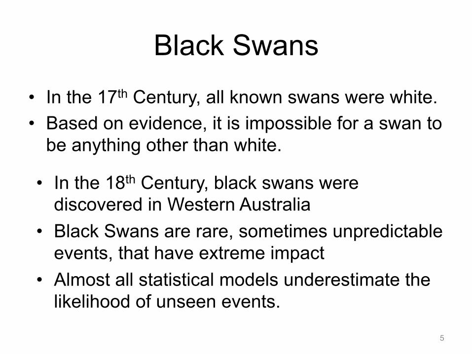
Black Swans

•  In the 17th Century, all known swans were white. •  Based on evidence, it is impossible for a swan to

be anything other than white.

5

•  In the 18th Century, black swans were discovered in Western Australia

•  Black Swans are rare, sometimes unpredictable events, that have extreme impact

•  Almost all statistical models underestimate the likelihood of unseen events.

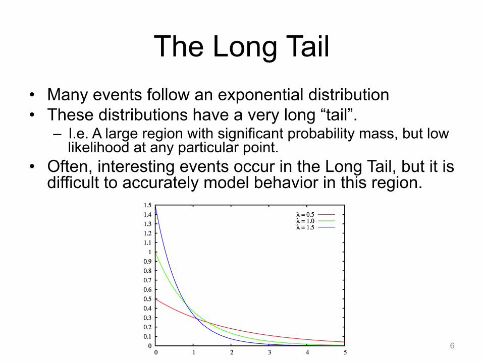
The Long Tail •  Many events follow an exponential distribution •  These distributions have a very long “tail”.

–  I.e. A large region with significant probability mass, but low likelihood at any particular point.

•  Often, interesting events occur in the Long Tail, but it is difficult to accurately model behavior in this region.

6

Boxes and Balls

•  2 Boxes, one red and one blue. •  Each contain colored balls.

7

Boxes and Balls

•  Suppose we randomly select a box, then randomly draw a ball from that box.

•  The identity of the Box is a random variable, B.

•  The identity of the ball is a random variable, L.

•  B can take 2 values, r, or b •  L can take 2 values, g or o.

8

Boxes and Balls

•  Given some information about B and L, we want to ask questions about the likelihood of different events.

•  What is the probability of selecting an apple?

•  If I chose an orange ball, what is the probability that I chose from the blue box?

9

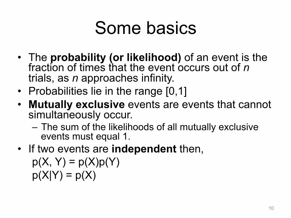
Some basics •  The probability (or likelihood) of an event is the

fraction of times that the event occurs out of n trials, as n approaches infinity.

•  Probabilities lie in the range [0,1] •  Mutually exclusive events are events that cannot

simultaneously occur. –  The sum of the likelihoods of all mutually exclusive

events must equal 1. •  If two events are independent then,

p(X, Y) = p(X)p(Y) p(X|Y) = p(X)

10

Joint Probability – P(X,Y) •  A Joint Probability function defines the likelihood of two

(or more) events occurring.

•  Let nij be the number of times event i and event j simultaneously occur.

11

p(X = xi, Y = yi) =nij

N

Orange Green Blue box 1 3 4 Red box 6 2 8

7 5 12

Generalizing the Joint Probability

12

�

i

�

j

nij = N

nij

cj =�

i

nij

ri =�

j

nij

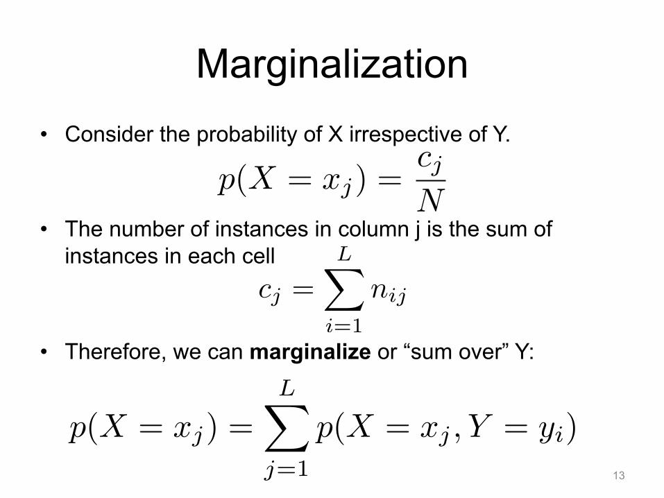
Marginalization •  Consider the probability of X irrespective of Y.

•  The number of instances in column j is the sum of instances in each cell

•  Therefore, we can marginalize or “sum over” Y:

13

cj =L�

i=1

nij

p(X = xj) =L�

j=1

p(X = xj , Y = yi)

p(X = xj) =cjN

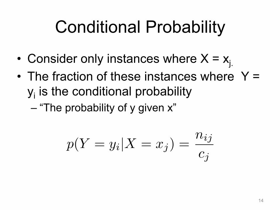
Conditional Probability

•  Consider only instances where X = xj. •  The fraction of these instances where Y =

yi is the conditional probability –  “The probability of y given x”

14

p(Y = yi|X = xj) =nij

cj

Relating the Joint, Conditional and Marginal

15

p(X = xi, Y = yj) =nij

N=

nij

ci· ciN

= p(Y = yj |X = xi)p(X = xi)

Sum and Product Rules •  In general, we’ll refer to a distribution over a

random variable as p(X) and a distribution evaluated at a particular value as p(x).

16

p(X) =�

Y

p(X,Y )

p(X,Y ) = p(Y |X)p(X)

Sum Rule

Product Rule

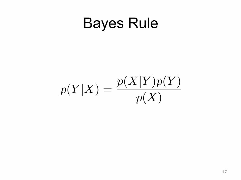
Bayes Rule

17

p(Y |X) =p(X|Y )p(Y )

p(X)

Interpretation of Bayes Rule

•  Prior: Information we have before observation.

•  Posterior: The distribution of Y after observing X

•  Likelihood: The likelihood of observing X given Y

18

p(Y |X) =p(X|Y )p(Y )

p(X)

Prior Posterior

Likelihood

Boxes and Balls with Bayes Rule

•  Assuming I’m inherently more likely to select the red box (66.6%) than the blue box (33.3%).

•  If I selected an orange ball, what is the likelihood that I selected the red box? – The blue box?

19

Boxes and Balls

20

p(B = r|L = o) =p(L = o|B = r)p(B = r)

p(L = o)

=6823712

=6

7

p(B = b|L = o) =p(L = o|B = b)p(B = b)

p(L = o)

=1413712

=1

7

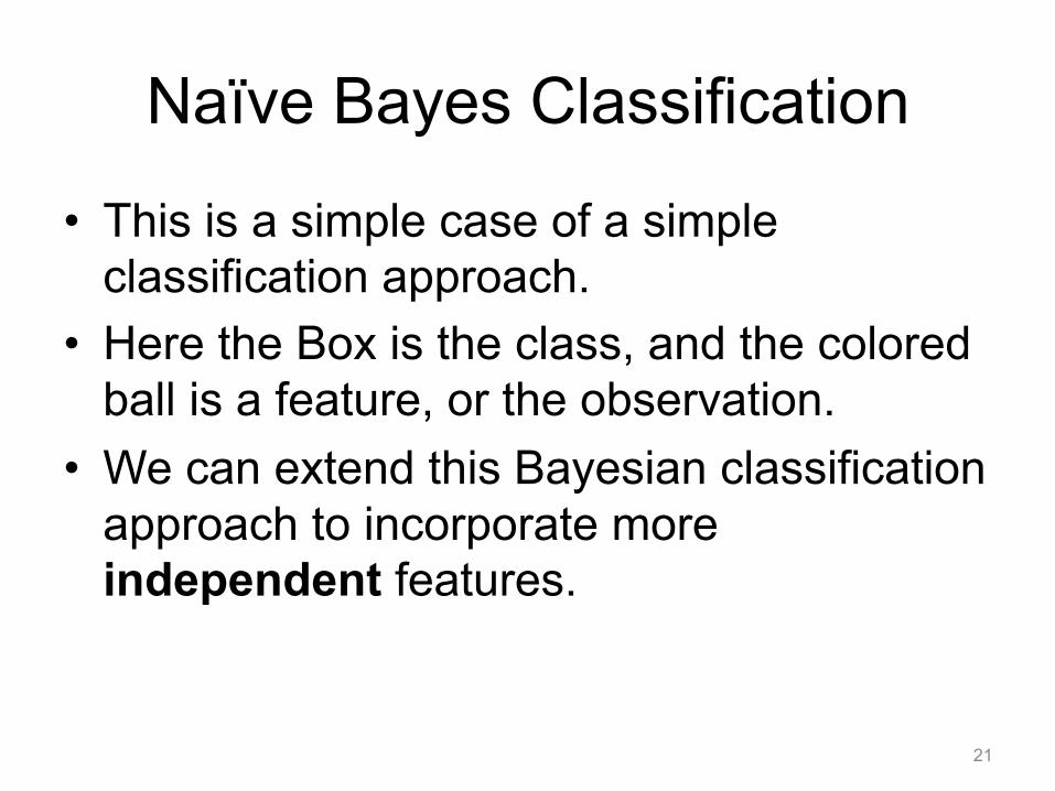
Naïve Bayes Classification

•  This is a simple case of a simple classification approach.

•  Here the Box is the class, and the colored ball is a feature, or the observation.

•  We can extend this Bayesian classification approach to incorporate more independent features.

21

Naïve Bayes Classification

•  Some theory first.

22

c∗ = argmaxc

p(x1, x2, . . . , xn|c)p(c)p(x1, x2, . . . , xn)

c∗ = argmaxc

p(c|x1, x2, . . . , xn)

p(x1, x2, . . . , xn|c) = p(x1|c)p(x2|c) · · · p(xn|c)

Naïve Bayes Classification

•  Assuming independent features simplifies the math.

23

c∗ = argmaxc

p(x1|c)p(x2|c) · · · p(xn|c)p(c)p(x1, x2, . . . , xn)

c∗ = argmaxc

p(x1|c)p(x2|c) · · · p(xn|c)p(c)

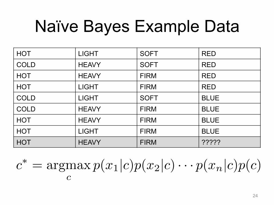
Naïve Bayes Example Data HOT LIGHT SOFT RED COLD HEAVY SOFT RED HOT HEAVY FIRM RED HOT LIGHT FIRM RED COLD LIGHT SOFT BLUE COLD HEAVY FIRM BLUE HOT HEAVY FIRM BLUE HOT LIGHT FIRM BLUE HOT HEAVY FIRM ?????

24

c∗ = argmaxc

p(x1|c)p(x2|c) · · · p(xn|c)p(c)

Naïve Bayes Example Data HOT LIGHT SOFT RED COLD HEAVY SOFT RED HOT HEAVY FIRM RED HOT LIGHT FIRM RED COLD LIGHT SOFT BLUE COLD HEAVY FIRM BLUE HOT HEAVY FIRM BLUE HOT LIGHT FIRM BLUE HOT HEAVY FIRM ?????

25

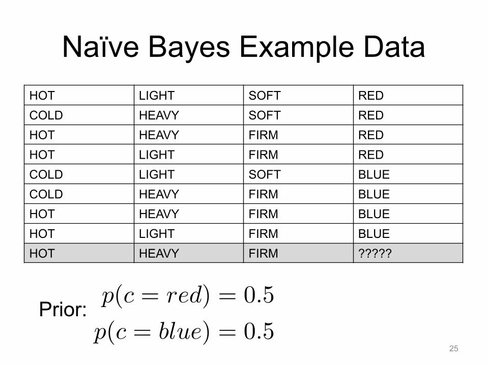
Prior: p(c = red) = 0.5

p(c = blue) = 0.5

Naïve Bayes Example Data HOT LIGHT SOFT RED COLD HEAVY SOFT RED HOT HEAVY FIRM RED HOT LIGHT FIRM RED COLD LIGHT SOFT BLUE COLD HEAVY SOFT BLUE HOT HEAVY FIRM BLUE HOT LIGHT FIRM BLUE HOT HEAVY FIRM ?????

26

p(hot|c = red) = 0.75

p(hot|c = blue) = 0.5

p(heavy|c = red) = 0.5

p(heavy|c = blue) = 0.5

p(firm|c = red) = 0.5

p(firm|c = blue) = 0.5

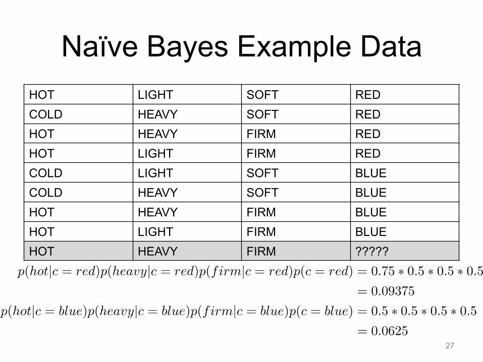
Naïve Bayes Example Data HOT LIGHT SOFT RED COLD HEAVY SOFT RED HOT HEAVY FIRM RED HOT LIGHT FIRM RED COLD LIGHT SOFT BLUE COLD HEAVY SOFT BLUE HOT HEAVY FIRM BLUE HOT LIGHT FIRM BLUE HOT HEAVY FIRM ?????

27

p(hot|c = red)p(heavy|c = red)p(firm|c = red)p(c = red) = 0.75 ∗ 0.5 ∗ 0.5 ∗ 0.5= 0.09375

p(hot|c = blue)p(heavy|c = blue)p(firm|c = blue)p(c = blue) = 0.5 ∗ 0.5 ∗ 0.5 ∗ 0.5= 0.0625

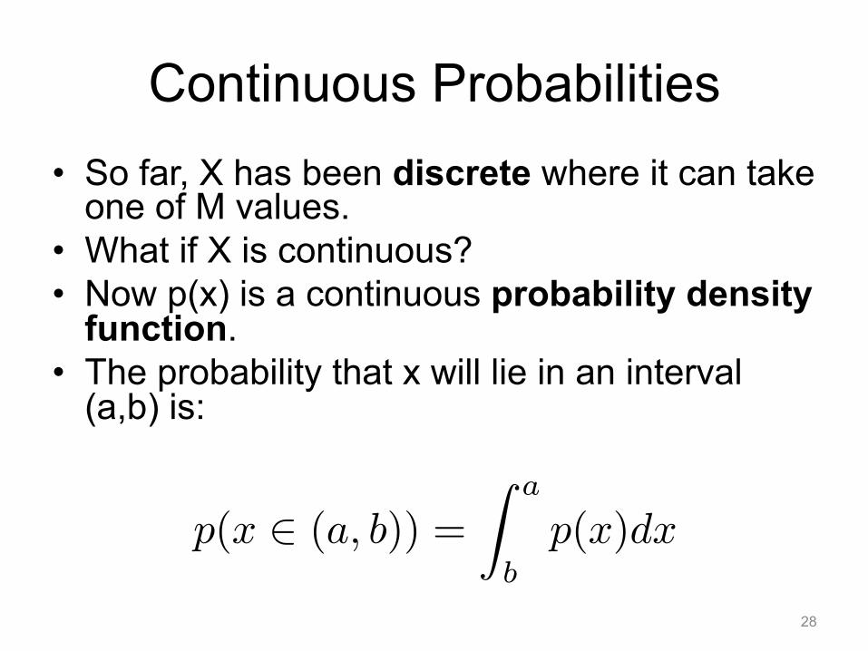
Continuous Probabilities •  So far, X has been discrete where it can take

one of M values. •  What if X is continuous? •  Now p(x) is a continuous probability density

function. •  The probability that x will lie in an interval

(a,b) is:

28

p(x ∈ (a, b)) =

� a

bp(x)dx

Continuous probability example

29

Properties of probability density functions

30

p(x) ≥ 1� ∞

−∞p(x)dx = 1

p(x) =

�p(x, y)dy

p(x, y) = p(y|x)p(x)

Sum Rule

Product Rule

Expected Values

•  Given a random variable, with a distribution p(X), what is the expected value of X?

31

E[x] =�

x

p(x)x

E[x] =�

p(x)xdx

Multinomial Distribution

•  If a variable, x, can take 1-of-K states, we represent the distribution of this variable as a multinomial distribution.

•  The probability of x being in state k is µk

32

K�

k=1

µk = 1 p(x;µ) =K�

k=1

µxkk

Expected Value of a Multinomial

•  The expected value is the mean values.

33

E[x;µ] =�

x

p(x;µ)x = (µ0, µ1, . . . , µK−1)T

Gaussian Distribution

•  One Dimension

•  D-Dimensions

34

N(x;µ,σ2) =1√2πσ2

exp

�− 1

2σ2(x− µ)2

�

N(x|µ,Σ) = 1

(2π)D/2|Σ|1/2exp

�−1

2(x− µ)TΣ−1(x− µ)

�

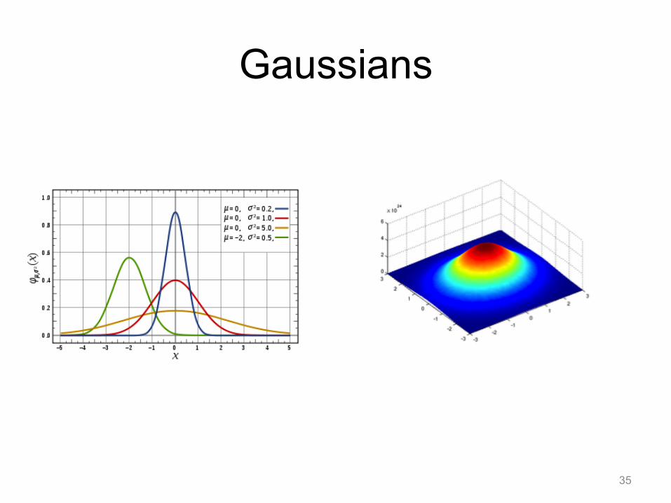
Gaussians

35

How machine learning uses statistical modeling

•  Expectation – The expected value of a function is the

hypothesis •  Variance

– The variance is the confidence in that hypothesis

36

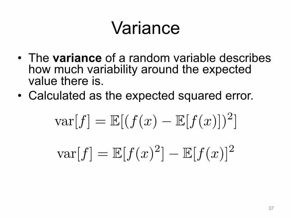
Variance •  The variance of a random variable describes

how much variability around the expected value there is.

•  Calculated as the expected squared error.

37

var[f ] = E[(f(x)− E[f(x)])2]

var[f ] = E[f(x)2]− E[f(x)]2

Covariance

•  The covariance of two random variables expresses how they vary together.

•  If two variables are independent, their covariance equals zero.

38

cov[x, y] = Ex,y[(x− E(x))(y − E[y])]= Ex,y[xy]− E[x]E[y]

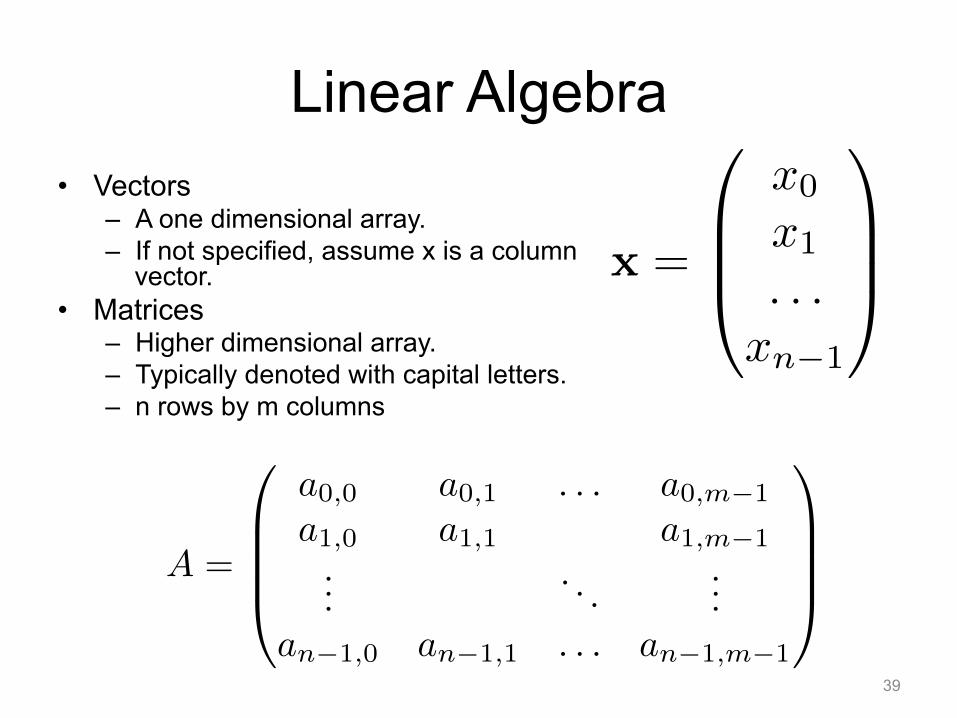
Linear Algebra •  Vectors

–  A one dimensional array. –  If not specified, assume x is a column

vector. •  Matrices

–  Higher dimensional array. –  Typically denoted with capital letters. –  n rows by m columns

39

x =

x0

x1

. . .xn−1

A =

a0,0 a0,1 . . . a0,m−1

a1,0 a1,1 a1,m−1...

. . ....

an−1,0 an−1,1 . . . an−1,m−1

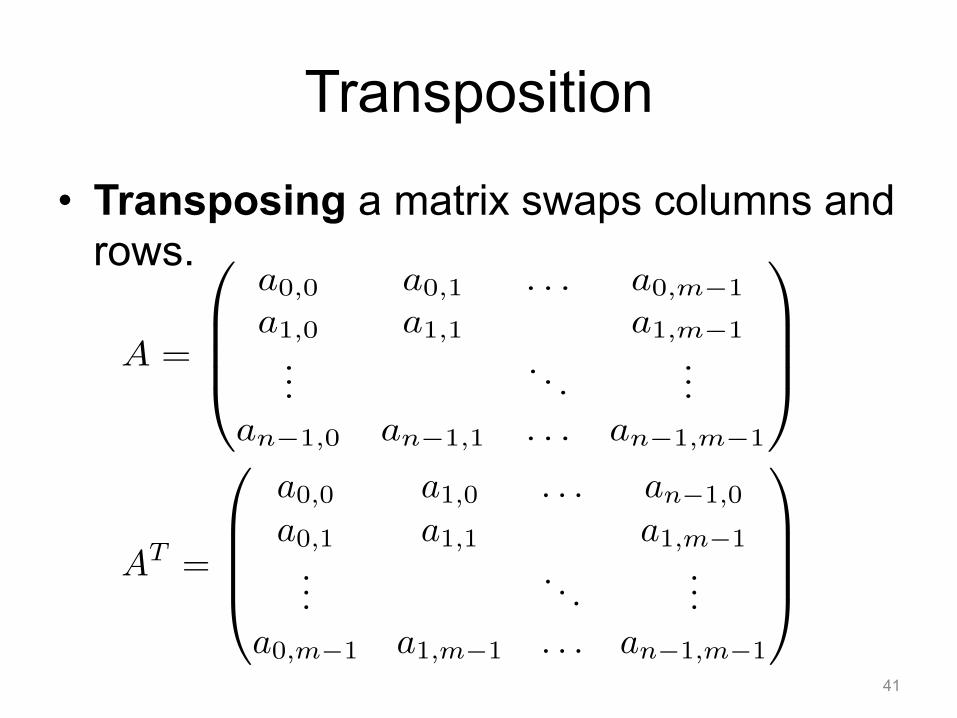
Transposition

•  Transposing a matrix swaps columns and rows.

40

xT =�x0 x1 . . . xn−1

�

x =

x0

x1

. . .xn−1

Transposition

•  Transposing a matrix swaps columns and rows.

41

A =

a0,0 a0,1 . . . a0,m−1

a1,0 a1,1 a1,m−1...

. . ....

an−1,0 an−1,1 . . . an−1,m−1

AT =

a0,0 a1,0 . . . an−1,0

a0,1 a1,1 a1,m−1...

. . ....

a0,m−1 a1,m−1 . . . an−1,m−1

Addition

•  Matrices can be added to themselves iff they have the same dimensions. – A and B are both n-by-m matrices.

42

A+B =

a0,0 + b0,0 a0,1 + b0,1 . . . a0,m−1 + b0,m−1

a1,0 + b1,0 a1,1 + b1,1 a1,m−1 + b1,m−1...

. . ....

an−1,0 + bn−1,0 an−1,1 + bn−1,1 . . . an−1,m−1 + bn−1,m−1

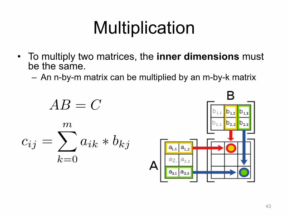
Multiplication •  To multiply two matrices, the inner dimensions must

be the same. –  An n-by-m matrix can be multiplied by an m-by-k matrix

43

AB = C

cij =m�

k=0

aik ∗ bkj

Inversion

•  The inverse of an n-by-n or square matrix A is denoted A-1, and has the following property.

•  Where I is the identity matrix is an n-by-n matrix with ones along the diagonal. –  Iij = 1 iff i = j, 0 otherwise

44

AA−1 = I

Identity Matrix

•  Matrices are invariant under multiplication by the identity matrix.

45

AI = A

IA = A

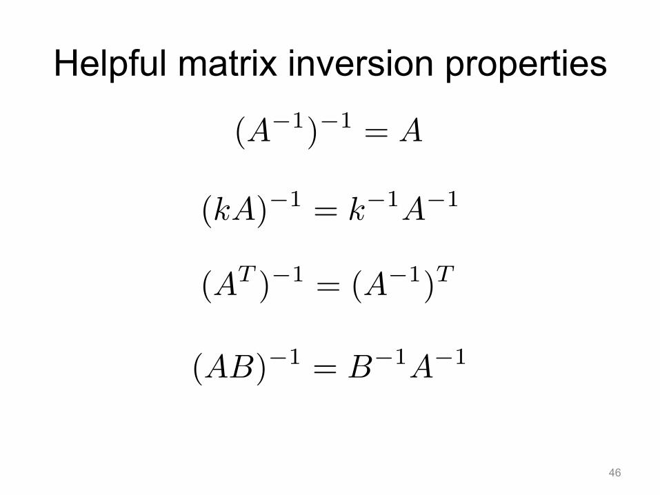
Helpful matrix inversion properties

46

(A−1)−1 = A

(kA)−1 = k−1A−1

(AT )−1 = (A−1)T

(AB)−1 = B−1A−1

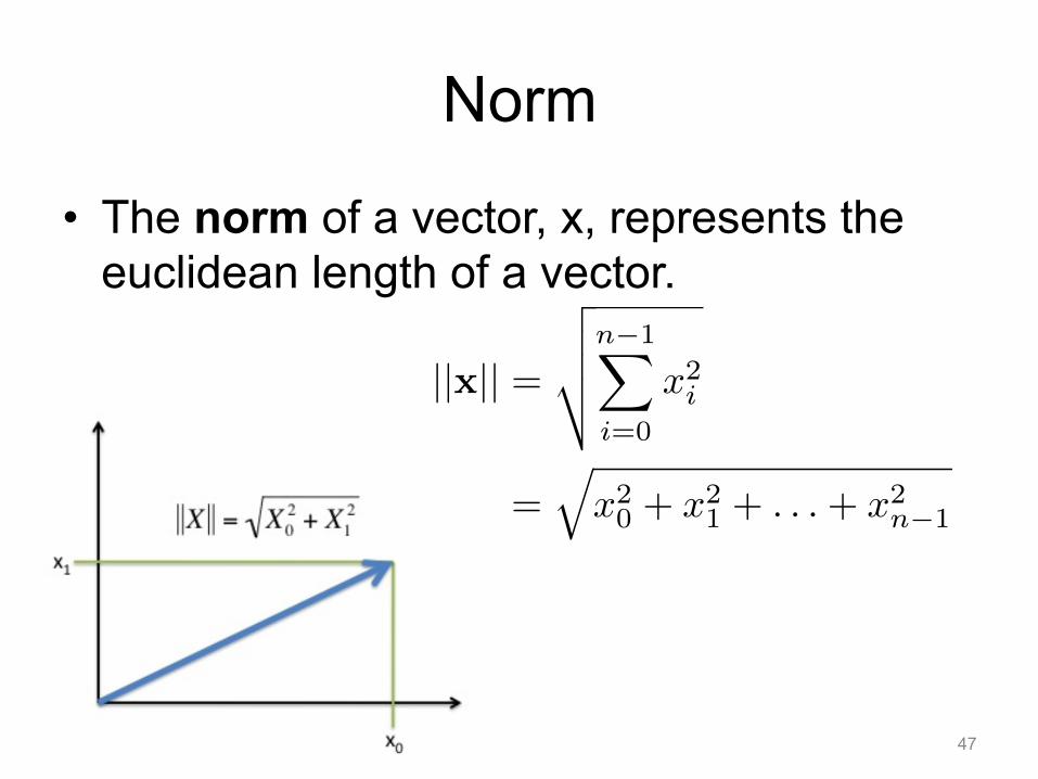
Norm

•  The norm of a vector, x, represents the euclidean length of a vector.

47

||x|| =

����n−1�

i=0

x2i

=�x20 + x2

1 + . . .+ x2n−1

Positive Definite-ness

•  Quadratic form – Scalar

– Vector

•  Positive Definite matrix M

•  Positive Semi-definite

48

c0 + c1x+ c2x2

xTAx

xTMx > 0

xTMx ≥ 0

Calculus

•  Derivatives and Integrals •  Optimization

49

Derivatives

•  A derivative of a function defines the slope at a point x.

50

d

dxf(x) or f �(x)

Derivative Example

51

Integrals

•  Integration is the inverse operation of derivation (plus a constant)

•  Graphically, an integral can be considered the area under the curve defined by f(x)

52

�f(x)dx = F (x) + c

F �(x) = f(x)

Integration Example

53

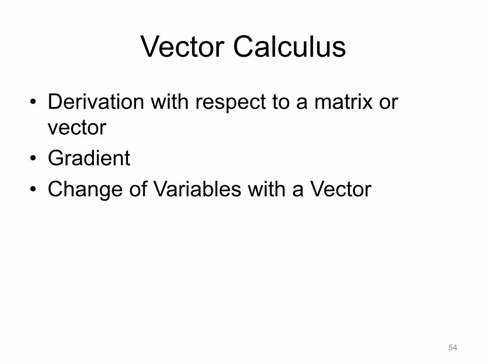
Vector Calculus

•  Derivation with respect to a matrix or vector

•  Gradient •  Change of Variables with a Vector

54

Derivative w.r.t. a vector

•  Given a vector x, and a function f(x), how can we find f’(x)?

55

f(x) : Rn → R

Derivative w.r.t. a vector

•  Given a vector x, and a function f(x), how can we find f’(x)?

56

f(x) : Rn → R

∂f(x)

∂x=

∂f(x)∂x0

∂f(x)∂x1

...∂f(x)∂xn−1

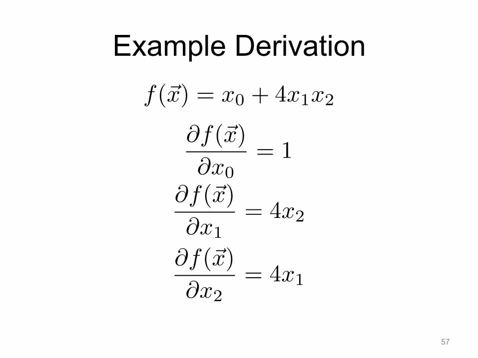
Example Derivation

57

f(�x) = x0 + 4x1x2

∂f(�x)

∂x0= 1

∂f(�x)

∂x1= 4x2

∂f(�x)

∂x2= 4x1

Example Derivation

58

f(�x) = x0 + 4x1x2

∂f(x)

∂x=

∂f(x)∂x0

∂f(x)∂x1

∂f(x)∂x2

=

1

4x2

4x1

Also referred to as the gradient of a function.

∇f(x) or ∇f

Useful Vector Calculus identities

•  Scalar Multiplication

•  Product Rule

59

∂

∂�x(�xT�a) =

∂

∂�x(�aT�x) = �a

∂

∂x(AB) =

∂A

∂xB +A

∂B

∂x∂

∂x(xTA) = A

∂

∂x(Ax) = AT

Useful Vector Calculus identities

•  Derivative of an inverse

•  Change of Variable

60

∂

∂x(A−1) = −A−1 ∂A

∂xA−1

�f(�x)d�x =

�f(�u)

����∂�x

∂�u

���� d�u

Optimization

•  Have an objective function that we’d like to maximize or minimize, f(x)

•  Set the first derivative to zero.

61

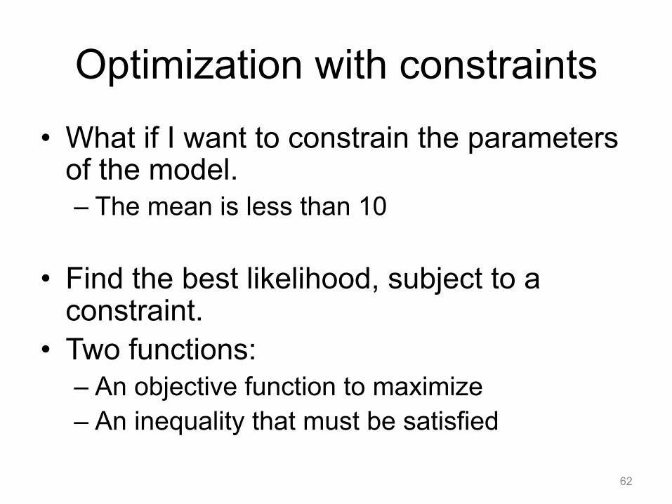
Optimization with constraints

•  What if I want to constrain the parameters of the model. – The mean is less than 10

•  Find the best likelihood, subject to a constraint.

•  Two functions: – An objective function to maximize – An inequality that must be satisfied

62

Lagrange Multipliers

•  Find maxima of f(x,y) subject to a constraint.

63

f(x, y) = x+ 2y

x2 + y2 = 1

General form

•  Maximizing:

•  Subject to:

•  Introduce a new variable, and find a maxima.

64

f(x, y)

g(x, y) = c

Λ(x, y,λ) = f(x, y) + λ(g(x, y)− c)

Example

•  Maximizing:

•  Subject to:

•  Introduce a new variable, and find a maxima.

65

f(x, y) = x+ 2y

x2 + y2 = 1

Λ(x, y,λ) = x+ 2y + λ(x2 + y2 − 1)

Example

66

∂Λ(x, y,λ)

∂x= 1 + 2λx = 0

∂Λ(x, y,λ)

∂y= 2 + 2λy = 0

∂Λ(x, y,λ)

∂λ= (x2 + y2 − 1) = 0

Now have 3 equations with 3 unknowns.

Example

67

1 = 2λx

2 = 2λy

1

x= 2λ =

2

y

y = 2x

Eliminate Lambda Substitute and Solve

x2 + y2 = 1

x2 + (2x)2 = 1

5x2 = 1

x = ± 1√5

y = ± 2√5

Why does Machine Learning need these tools?

•  Calculus – We need to identify the maximum likelihood, or

minimum risk. Optimization –  Integration allows the marginalization of

continuous probability density functions •  Linear Algebra

– Many features leads to high dimensional spaces – Vectors and matrices allow us to compactly

describe and manipulate high dimension al feature spaces.

68

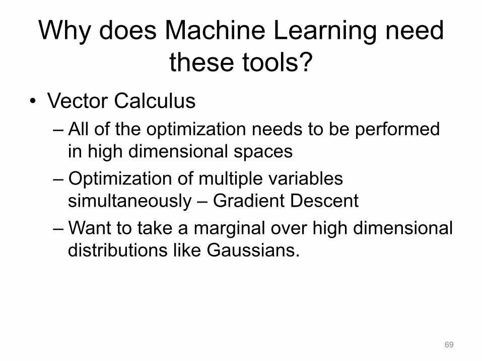
Why does Machine Learning need these tools?

•  Vector Calculus – All of the optimization needs to be performed

in high dimensional spaces – Optimization of multiple variables

simultaneously – Gradient Descent – Want to take a marginal over high dimensional

distributions like Gaussians.

69

Next Time

•  Linear Regression and Regularization

•  Read Chapter 1.1, 3.1, 3.3

70