probabilistic tomography of atmospheric parameters from gnss...
TRANSCRIPT
Alma Mater Studiorum - Universita di Bologna
DOTTORATO DI RICERCA
MODELLISTICA FISICA PER LA PROTEZIONE DELL’AMBIENTE
Ciclo XXII
Settore scientifico-disciplinare di afferenza: FIS/06
Probabilistic Tomographyof Atmospheric parameters from
GNSS data
Presentata da: Relatore:Dott. Alberto Ortolani Prof. Rolando Rizzi
Coordinatore:Prof. Rolando Rizzi
Esame finale anno 2011

ii

Alla mia piccola Irene,
al tempo che non abbiamo avuto
e a quello che passeremo insieme,
altrove.
To my little Irene,
to the time that we haven’t had
and to the one we will spend together,
elsewhere.
iii

iv
Contents
Introduction 1
1 Stationary view of the Earth atmosphere 5
1.1 Basic assumptions . . . . . . . . . . . . . . . . . . . . . . . . . . . 5
1.2 Neutral atmosphere . . . . . . . . . . . . . . . . . . . . . . . . . . 6
1.2.1 Thermal classification of the atmosphere . . . . . . . . . . 6
1.2.2 Standard atmosphere . . . . . . . . . . . . . . . . . . . . . 12
1.2.3 Water vapour distribution and laws . . . . . . . . . . . . . 16
1.3 Non neutral atmosphere . . . . . . . . . . . . . . . . . . . . . . . 17
1.3.1 Plasma component of the atmosphere . . . . . . . . . . . . 17
1.3.2 Ionosphere classification . . . . . . . . . . . . . . . . . . . 18
2 Atmospheric effects on GNSS signals 23
2.1 Propagating electromagnetic signals . . . . . . . . . . . . . . . . . 23
2.2 Electromagnetic signals in gas media . . . . . . . . . . . . . . . . 25
2.2.1 Interaction with a neutral non-polarised gas . . . . . . . . 25
2.2.2 Interaction with a neutral but polarised gas . . . . . . . . 34
2.2.3 Interaction with a ionised gas . . . . . . . . . . . . . . . . 39
2.3 Signal delay . . . . . . . . . . . . . . . . . . . . . . . . . . . . . . 43
2.3.1 Delay components . . . . . . . . . . . . . . . . . . . . . . 43
2.3.2 Bending . . . . . . . . . . . . . . . . . . . . . . . . . . . . 47
2.3.3 Simulations . . . . . . . . . . . . . . . . . . . . . . . . . . 50
v
3 The GPS satellite navigation system 57
3.1 The basis of satellite navigation . . . . . . . . . . . . . . . . . . . 57
3.2 GPS constellation . . . . . . . . . . . . . . . . . . . . . . . . . . . 59
3.2.1 Space segment structure . . . . . . . . . . . . . . . . . . . 59
3.2.2 Building up of the GPS constellation . . . . . . . . . . . . 60
3.2.3 Satellite instruments . . . . . . . . . . . . . . . . . . . . . 62
3.3 GPS signal . . . . . . . . . . . . . . . . . . . . . . . . . . . . . . . 65
3.3.1 Pseudorange measurements . . . . . . . . . . . . . . . . . 68
3.3.2 Carrier phase measurements . . . . . . . . . . . . . . . . . 70
3.4 Components of the apparent signal travel-time . . . . . . . . . . . 72
3.4.1 Tropospheric delay . . . . . . . . . . . . . . . . . . . . . . 72
3.4.2 Ionospheric delay . . . . . . . . . . . . . . . . . . . . . . . 73
3.4.3 Relativistic effects . . . . . . . . . . . . . . . . . . . . . . . 74
3.4.4 Instrumental delays and differential code biases . . . . . . 76
3.4.5 Orbit parameters errors . . . . . . . . . . . . . . . . . . . 79
3.4.6 Earth rotation: the Sagnac effect . . . . . . . . . . . . . . 84
3.4.7 Satellite clock offsets and drifts . . . . . . . . . . . . . . . 85
3.4.8 Receiver clock errors . . . . . . . . . . . . . . . . . . . . . 86
3.4.9 Multipath . . . . . . . . . . . . . . . . . . . . . . . . . . . 89
3.4.10 Additional error sources . . . . . . . . . . . . . . . . . . . 90
3.5 Other GNSS systems . . . . . . . . . . . . . . . . . . . . . . . . . 91
3.5.1 GLONASS . . . . . . . . . . . . . . . . . . . . . . . . . . . 91
3.5.2 Galileo . . . . . . . . . . . . . . . . . . . . . . . . . . . . . 92
3.5.3 Complementarity and interoperability . . . . . . . . . . . . 94
4 Retrieval of atmospheric profiles 97
4.1 Classical approaches for GNSS WV retrieval . . . . . . . . . . . . 97
4.2 Classical tomographic recontruction problem . . . . . . . . . . . . 102
4.3 A probabilistic approach to atm. tomography . . . . . . . . . . . 108
4.3.1 1D retrievals . . . . . . . . . . . . . . . . . . . . . . . . . . 109
vi
4.3.2 Extension to 3D retrievals . . . . . . . . . . . . . . . . . . 116
4.4 Numerical experiments . . . . . . . . . . . . . . . . . . . . . . . . 117
4.4.1 Basic data . . . . . . . . . . . . . . . . . . . . . . . . . . . 118
4.4.2 Generation of a synthetic database . . . . . . . . . . . . . 119
4.4.3 Entropy and information . . . . . . . . . . . . . . . . . . . 123
4.4.4 Results of numerical experiments . . . . . . . . . . . . . . 126
5 Lines of future development 139
5.1 Improvement of the a priori dataset . . . . . . . . . . . . . . . . . 139
5.2 Shape of the error probability functions . . . . . . . . . . . . . . . 140
5.3 Transition to continuous variables . . . . . . . . . . . . . . . . . . 141
5.4 Upgrading to a 4D processing . . . . . . . . . . . . . . . . . . . . 142
5.5 Growing the state vectors for new measurements . . . . . . . . . . 143
Conclusions 147
Bibliography 151
*
vii

viii
List of Figures
1.1 Atmospheric hydrostatic vertical balance. . . . . . . . . . . . . . . 6
1.2 Typical vertical profiles of density and pressure. . . . . . . . . . . 7
1.3 Temperature profile and principal chemical components in atmo-
sphere. . . . . . . . . . . . . . . . . . . . . . . . . . . . . . . . . . 8
1.4 Atmospheric radiative transmission. . . . . . . . . . . . . . . . . . 8
1.5 Vertical profile of thermal conductivity for dry air. . . . . . . . . . 19
1.6 Average ionospheric densities. . . . . . . . . . . . . . . . . . . . . 19
1.7 Mean free path of particles in atmosphere. . . . . . . . . . . . . . 20
2.1 Geometry of a plane wave. . . . . . . . . . . . . . . . . . . . . . . 24
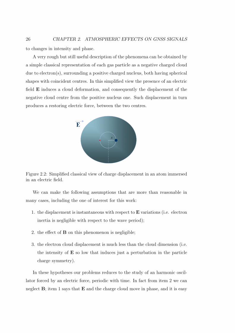
2.2 Simplified classical view of charge displacement in an atom im-
mersed in an electric field. . . . . . . . . . . . . . . . . . . . . . . 26
2.3 Geometry of the emitting dipole. . . . . . . . . . . . . . . . . . . 28
2.4 Layer of atmosphere of quasi-infinitesimal thickness crossed by an
electromagnetic signal. . . . . . . . . . . . . . . . . . . . . . . . . 30
2.5 Dipole of the water vapour molecule in an electric field. . . . . . . 35
2.6 Values of compressibility factors at different heights. . . . . . . . . 39
2.7 Bending geometry for a plane parallel atmosphere. . . . . . . . . . 49
2.8 Bending geometry in polar coordinates. . . . . . . . . . . . . . . . 49
2.9 Increment of integrated atmospheric delays for GNSS signals along
zenith paths. . . . . . . . . . . . . . . . . . . . . . . . . . . . . . 52
2.10 Simulation of path parameters for different elevation angles in a
standard troposphere. . . . . . . . . . . . . . . . . . . . . . . . . . 54
ix
2.11 Different ray trajectories and distances between straight and curved
paths due to the bending in a standard troposphere. . . . . . . . . 55
3.1 Typical Oscillator Stabilities expressed as Allan variances. . . . . 64
3.2 Typical Allan deviations of caesium clocks and quartz oscillators. 65
3.3 Scheme of the GPS satellite signal structure. . . . . . . . . . . . . 66
3.4 PRNs crosscorrelation and autocorrelation examples. . . . . . . . 68
3.5 Comparison between dual frequencies ionospheric delays affected
by receiver biases and corresponding ionospheric delays from Klobuchar
model data. . . . . . . . . . . . . . . . . . . . . . . . . . . . . . . 80
3.6 Ephemeris error components. . . . . . . . . . . . . . . . . . . . . 81
3.7 ECEF reference system rotation due to Earth rotation. . . . . . . 85
3.8 Stability of TCXO and OCXO clock crystals. . . . . . . . . . . . 88
3.9 Structure of the Galileo Navigation Signal. . . . . . . . . . . . . . 93
4.1 Geometry of data acquisition in a tomography problem. . . . . . . 104
4.2 Sketches of GNSS measurement geometries for atmospheric to-
mography. . . . . . . . . . . . . . . . . . . . . . . . . . . . . . . . 107
4.3 Example of correlated adimensional variables for two levels before
and after orthogonalisation. . . . . . . . . . . . . . . . . . . . . . 115
4.4 Distribution of temperature and water vapour pressure at different
pressure levels. . . . . . . . . . . . . . . . . . . . . . . . . . . . . 118
4.5 GFS profiles. . . . . . . . . . . . . . . . . . . . . . . . . . . . . . 120
4.6 Distributions of original and synthetic data. . . . . . . . . . . . . 121
4.7 Distributions of synthetic data at different layers. . . . . . . . . . 122
4.8 Artificial supersaturated states. . . . . . . . . . . . . . . . . . . . 123
4.9 Effectiveness of absolute and relative entropy in measuring varia-
tions in distribution functions. . . . . . . . . . . . . . . . . . . . . 126
4.10 Eigenvalues of the covariance matrix. . . . . . . . . . . . . . . . . 128
4.11 Entropies measured for the target parameters above FI. . . . . . . 133
4.12 Relative entropies measured for the target parameters above FI. . 134
x
4.13 Example of a state vector retrieval. . . . . . . . . . . . . . . . . . 135
4.14 Entropies measured for the target parameters above FI with mea-
surements also in SI. . . . . . . . . . . . . . . . . . . . . . . . . . 136
4.15 Relative entropies measured for the target parameters above FI
with measurements also in SI. . . . . . . . . . . . . . . . . . . . . 137
xi

xii

List of Tables
1.1 Concentrations of main atmospheric gases. . . . . . . . . . . . . . 7
xiii

xiv
List of Acronyms
APL: Applied Physics Laboratory
A-S: Anti-Spoof
AUTONAV: AUTOnomous NAVigation
BPSK: Binary Phase Shift Keying
CDMA: Code Division Multiple Access
COSMEMOS: COoperative Satellite navigation for MEteo-marine MOdelling
and Services
CS: Control Segment
CS: Commercial Service
DCB: Differential Code Bias
ECEF: Earth Centred Earth Fixed
ECI: Earth Centred Inertial
ECMWF: European Centre for Medium Range Weather Forecasts
EO: Earth Observation
EOF: Empirical Orthogonal Function
FDMA: Frequency Division Multiple Access
xv

FP7: 7th Framework Programme
GA: Ground Antenna
GFS: Global Forecast System
GLONASS: GLObal NAvigation Satellite System
GNSS: Global Navigation Satellite System
GPS : Global Positioning System
IEEE: Institute for Electrical and Electronic Engineers
IGS: International GPS Service for Geodynamics
IR: InfraRed
IRNSS: Indian Regional Navigational Satellite System
IWV: Integrated Water Vapor
LAM: Limited Area Model
MCS: Master Control Station
MEO: Medium Earth Orbit
MS: Monitor Station
MW: MicroWaves
NAVSTAR: NAVigation System with Time And Ranging
NAVWAR: NAVigation WARfare
NGS: National Geodetic Survey
NCST: Naval Center for Space Technology
NDS: Nuclear detonation Detection System
xvi

NNSS: Navy Navigation Satellite System
NRL: Naval Research Laboratory
NWP: Numerical Weather Prediction
OCS: Operational Control Segment
OCXO: Oven Controlled Crystal Oscillator
OS: Open Service
PPS: Precise Positioning Service
PRN: Pseudo Random Noise
PRS: Public Regulated Service
PW: Precipitable Water
RC: Ranging Codes
RH: Relative Humidity
RHCP: Right-Hand Circularly Polarised
SA: Selective Availability
SAR: Search And Resque
SBAS: Satellite Based Augmentation System
SOL: Safety Of Life
SSM: Spread Spectrum Modulation
SPS: Standard Position Service
TCXO: Temperature Compensated Crystal Oscillator
TEC: Total Electron Content
xvii
TIMATION: TIMe navigATION
UV: UltraViolet
WMO: World Meteorological Organisation
WRF: Weather Research and Forecasting
ZHD: Zenith Hydrostatic Delay
ZWD: Zenith Wet Delay
xviii
Introduction
Problem statement
In the next few years, as soon as Galileo will be deployed, more than 50 GNSS
(Global Navigation Satellite System) and SBAS (Satellite Based Augmentation
System) satellites will be operational, emitting precise microwave (MW) L-band
spread spectrum signals, and will remain in operation for several decades. As
it will be comprehensively described in this work, these signals, can be used for
remote sensing of the Earth, distinctively for atmospheric monitoring.
A number of works are available for measuring vertically integrated water-
vapour, sometime referred as precipitable water, from fixed GNSS receiving sta-
tions (see for instance Bar-Sever 1997). They generally propose different solu-
tions to the problem, but the basic idea they are based on is essentially the
following: computing the signal delay due to the geometric distance between
satellites and the receiver station, whose position is know with great accuracy
(being fixed); then measuring the actual phase-delay of the GNSS signal (mea-
sured by the receiver); finally subtracting the delay for the geometric distance,
in order to obtain the delay due to atmospheric effects. The problem of esti-
mating water vapour is however much more complicated, because such delay
contains also various errors due to uncertainties in satellite and receiver clocks,
relativistic effects, receiver processing steps etc. (J. J. Spilker, Jr, 1980; B.W.
Parkinson, J.J. Spilker, 1996), that often are of the same order of magnitude
of the atmospheric effects we want to measure, and very difficult to model with
the necessary accuracy. In addition the atmospheric delay consist of a first ma-
jor term from ionospheric effects, a second term from the dry component of the
1
2
troposphere and a third term from the water vapour (i.e. the wet part), that
have to be decoupled. The Ionosphere is dispersive at the GNSS frequencies,
thus a receiver processing the different GNSS frequencies allows to decouple the
ionospheric components, by forming the ionospheric-free combination. In order
to decouple the dry tropospheric effects, some ancillary information are needed.
Normally a number of strong approximations are done in order to solve the prob-
lem. Typically, mapping functions are used to map slant tropospheric delay into
zenith delay, and inferences on the temperature and pressure vertical profiles
are made from local measurements in order to close the system equations in the
retrieval process (Bevis et al. 1992; Rocken et al. 1995).
The aim of the present work is to demonstrate that, under certain conditions
and through a proper bayesian approach, profiles (instead of integrated values) of
water-vapour partial pressure, of temperature and pressure are achievable from
GNSS data. We will show that a 3D retrieval (into a limited volume) of such
atmospheric parameters could be achievable through a simultaneous processing
of GNSS signals from different receivers. These are key parameters in meteorol-
ogy, because they are the basic tropospheric state parameters, driving the local
dynamics, the precipitation and the exchange of latent and sensible heat between
atmosphere and earth surface. A probabilistic algorithm is thus proposed, that
goes beyond the “mapping function approach” for measuring zenith integrated
atmospheric parameters, i.e. averaged parameters in a strict plane parallel ap-
proximation for atmosphere. The issue we want to address is analogous to the
“classical” tomography problem, but from measurements of GNSS delays sam-
pled from station points and for slant directions that are inhomogeneous in space
and variable in time: as a consequence the properties of discrete Fourier trans-
forms are not (at least straightforwardly) exploitable, as normally it is done to
solve the tomographic problem.
It will be analysed on which extent the accuracy of retrievals depends on
precisions and number of available signals (i.e. of satellites simultaneously in
view and receivers in the target area) and on ancillary information eventually

3
available, such as measurements of surface pressure, temperature and relative
humidity. As a main achievement however it will be assessed where information
is effectively gained due to GNSS data, with respect to a priori information or in
situ measurements. Not surprisingly the assessment of water vapour is the most
positively constrained by GNSS data, but, under some conditions and measure-
ment configurations, also temperature and even pressure can gain information,
especially for non surface values.
The core part of such analysis is performed in a “controlled environment”,
i.e. it is done by means of synthetic data that however are generated on the
basis of a previous accurate analysis of main characteristics of real data, errors
included.
The proposed approach has the advantage to retrieve parameters each time
with their probability density functions (i.e. uncertainties), as mandatory, for
example, for a correct assimilation into models. In the perspective of an even-
tual operational implementation the method has a second advantage, that is the
robustness, because number, distribution and precision of measurements affect
result accuracy but not the feasibility of the retrieval process, that, at worst, it
gives back a priori distributions. Conversely it can be very machine-time con-
suming, if some expedients are not adopted, especially in case of large number
of measurements to be processed.
Structure of the thesis
The structure of the thesis is the following:
• Chapter 1 recalls the basics characteristics of the atmosphere from a sta-
tionary point of view, with more details on troposphere and ionosphere,
that are relevant for the present work as the basis of the a priori knowledge
of the parameters we want to retrieve.
• Chapter 2 analyses the properties of an electromagnetic L-band wave cross-
ing a gas medium (neutral and slightly ionised), up to evaluating approxi-
4
mations enclosed in the geometrical optics approach we adopt as solution
to the problem.
• Chapter 3 describes the principles of GNSS positioning signals, and, re-
ferring mainly to GPS, the main error sources in the computation of the
tropospheric component of the signal delay from fixed receiving stations.
• Chapter 4 explains the algorithm designed for retrieving the atmospheric
parameters from the GNSS tropospheric delays, addressing the problem
from 0D to 3D, and it describes also the dataset generated for testing
performances and information content achievable through different mea-
surement configurations.
• Chapter 5 looks beyond the present work, suggesting future development
of the approach and application to new EO contexts.
Subjects of relevance for the work, but that are not essential in its logic flow,
are dealt in specific notes instead of appendixes, in order to keep them close to
the main arguments they are related to.
Chapter 1
Stationary view of the Earthatmosphere
1.1 Basic assumptions
The atmosphere is essentially a gaseous shell surrounding the (solid and liquid)
Earth. It is a mixture of different gases, neutral for more than 99% in mass
(cf. [47]). Thermodynamics and Earth gravitation determine the gas density
at different height: a limit height of the shell can be arbitrarily set around
1000 km, where the gravitational field is about 30% of the surface value, the
average particle velocity (mainly due to UV solar radiation absorption) equals the
escape threshold (∼ 11 km/s), and the gas density is approximately 10−15 kg/m3
(with respect to about 1.2 kg/m3 at the sea level) (cf. [15]). The goodness of such
limit definition is of course dependent on the problem we are dealing with: in
our case we will see in § 2 that the effects on the signal delay at GPS (more
generally GNSS) frequencies (1÷ 2 GHz) due to the neutral and charged parts
of the atmosphere vanish even at lower heights than 1000 km.
In spite of the complexities of atmospheric phenomena, the majority of the
properties we are interested in can be described in the ideal gas approximation,
thus through the basic thermodynamics variables, i.e. temperature and partial
pressures of the different gas species (both neutral and charged ones).
5
6 CHAPTER 1. STATIONARY VIEW OF THE EARTH ATMOSPHERE
1.2 Neutral atmosphere
1.2.1 Thermal classification of the atmosphere
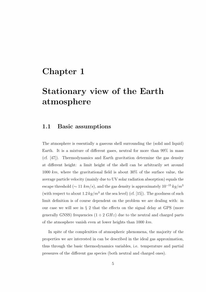
At the equilibrium, a gas in a gravitational field follows the hydrostatic law, with
pressure locally balancing the gravitational force. It can be written as a vector
differential equation and simplified to the scalar form if the problem is essentially
one dimensional, as it happens for the Earth atmosphere where the gravitational
field is (quasi) homogeneous (Fig. 1.1):
dP = −ρ · g dz (1.1)
with P , ρ and g, respectively pressure, density and gravitational acceleration
at height z. As a consequence the P gradient depends on g and on the local
temperature T , through ρ, according to the ideal gas law (cf. [18]):
P = R ρ T (1.2)
being R the gas constant1.
Figure 1.1: Atmospheric hydrostatic vertical balance.
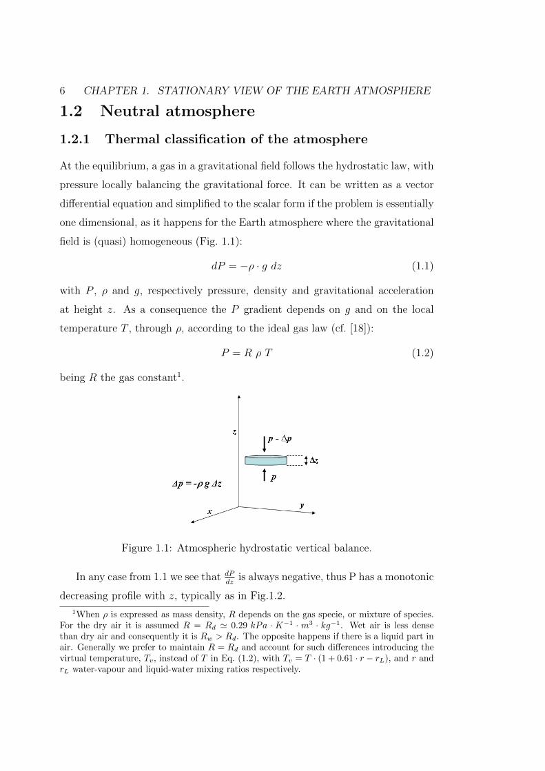
In any case from 1.1 we see that dPdz
is always negative, thus P has a monotonic
decreasing profile with z, typically as in Fig.1.2.
1When ρ is expressed as mass density, R depends on the gas specie, or mixture of species.For the dry air it is assumed R = Rd ' 0.29 kPa · K−1 · m3 · kg−1. Wet air is less densethan dry air and consequently it is Rw > Rd. The opposite happens if there is a liquid part inair. Generally we prefer to maintain R = Rd and account for such differences introducing thevirtual temperature, Tv, instead of T in Eq. (1.2), with Tv = T · (1 + 0.61 · r − rL), and r andrL water-vapour and liquid-water mixing ratios respectively.
1.2. NEUTRAL ATMOSPHERE 7
Figure 1.2: Typical vertical profiles of density and pressure (after [43]).
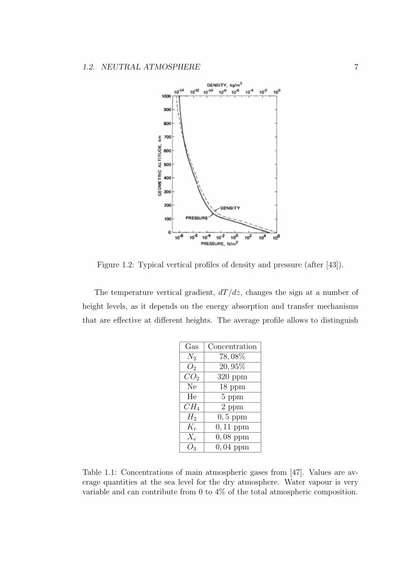
The temperature vertical gradient, dT/dz, changes the sign at a number of
height levels, as it depends on the energy absorption and transfer mechanisms
that are effective at different heights. The average profile allows to distinguish
Gas ConcentrationN2 78, 08%O2 20, 95%CO2 320 ppmNe 18 ppmHe 5 ppmCH4 2 ppmH2 0, 5 ppmKr 0, 11 ppmXe 0, 08 ppmO3 0, 04 ppm
Table 1.1: Concentrations of main atmospheric gases from [47]. Values are av-erage quantities at the sea level for the dry atmosphere. Water vapour is veryvariable and can contribute from 0 to 4% of the total atmospheric composition.
8 CHAPTER 1. STATIONARY VIEW OF THE EARTH ATMOSPHERE
Figure 1.3: Temperature profile and principal chemical components in atmo-sphere (after [27]).
Figure 1.4: Atmospheric radiative transmission.
four atmospheric regions (Fig.1.3): troposphere, stratosphere, mesosphere and
thermosphere.
1.2. NEUTRAL ATMOSPHERE 9
At the sea level the gas composition of the dry atmosphere is as in Tab. 1.1.
In the atmosphere there can be also a component of water vapour very variable,
spanning from 0 to 4% of the total atmospheric composition.
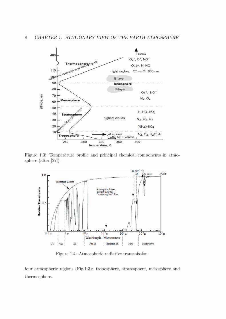
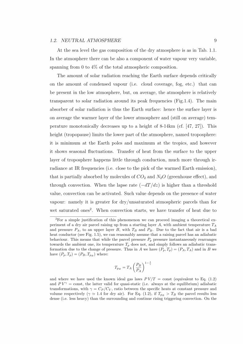
The amount of solar radiation reaching the Earth surface depends critically
on the amount of condensed vapour (i.e. cloud coverage, fog, etc.) that can
be present in the low atmosphere, but, on average, the atmosphere is relatively
transparent to solar radiation around its peak frequencies (Fig.1.4). The main
absorber of solar radiation is thus the Earth surface: hence the surface layer is
on average the warmer layer of the lower atmosphere and (still on average) tem-
perature monotonically decreases up to a height of 8-14km (cf. [47, 27]). This
height (tropopause) limits the lower part of the atmosphere, named troposphere:
it is minimum at the Earth poles and maximum at the tropics, and however
it shows seasonal fluctuations. Transfer of heat from the surface to the upper
layer of troposphere happens little through conduction, much more through ir-
radiance at IR frequencies (i.e. close to the pick of the warmed Earth emission),
that is partially absorbed by molecules of CO2 and N2O (greenhouse effect), and
through convection. When the lapse rate (−dT/dz) is higher than a threshold
value, convection can be activated. Such value depends on the presence of water
vapour: namely it is greater for dry/unsaturated atmospheric parcels than for
wet saturated ones2. When convection starts, we have transfer of heat due to
2For a simple justification of this phenomenon we can proceed imaging a theoretical ex-periment of a dry air parcel raising up from a starting layer A, with ambient temperature TAand pressure PA, to an upper layer B, with TB and PB . Due to the fact that air is a badheat conductor (see Fig. 1.5), we can reasonably assume that a raising parcel has an adiabaticbehaviour. This means that while the parcel pressure Pp pressure instantaneously rearrangestowards the ambient one, its temperature Tp does not, and simply follows an adiabatic trans-formation due to the change of pressure. Thus in A we have (Pp, Tp) = (PA, TA) and in B wehave (Pp, Tp) = (PB , TpB ) where:
TpB = TA
(PBPA
)1− 1γ
and where we have used the known ideal gas laws P V/T = const (equivalent to Eq. (1.2)and P V γ = const, the latter valid for quasi-static (i.e. always at the equilibrium) adiabatictransformations, with γ = CP /CV , ratio between the specific heats at constant pressure andvolume respectively (γ ' 1.4 for dry air). For Eq. (1.2), if TpB > TB the parcel results lessdense (i.e. less heavy) than the surrounding and continue rising triggering convection. On the
10 CHAPTER 1. STATIONARY VIEW OF THE EARTH ATMOSPHERE
vertical transport (thus mixing) of mass, ad in primis of water vapour, that evap-
orates from the Earth surface and that sometimes can be lifted to layers whose
temperature and pressure conditions can cause condensation and then precipita-
tion. This transport mechanism can be effective at different atmospheric levels
up to the whole troposphere, sometimes even overshooting the tropopause, into
the lower stratosphere, in these cases often associated to extreme precipitation
events.
When activated, convection is very efficient in transferring heat and in a
certain way it acts as stabiliser of the tropospheric lapse rate, preventing to
overpass the limit thresholds. In fact diurnal cycles and horizontal dynamics
(i.e. advections of air masses), continuously change the lapse rate with respect
to the average profiles, generating what are defined as meteorological events.
Above the tropopause the atmosphere is essentially stable, no matter of the
lapse rate sign. In particular the stratosphere has a positive temperature gradient
(i.e. a negative lapse rate), resulting exceptionally stable to vertical motions, that
practically are totally inhibited. Stratospheric warming is not linked to Earth
surface phenomena, but it depends more directly on solar radiation, namely UV
(0.1 ÷ 0.2 µm) absorption due to oxygen photodissociation: O2 + hν → 2O,
with hν energy of UV photons. In a height range of 20 ÷ 50 km the amount of
molecular oxygen sustains an exothermal reaction producing ozone, O2 + O →
O3, that in turn is an efficient UV radiation absorber, through the dissociation
O3 + hν → O2 + O.
contrary if TpB ≤ TB convection is inhibited.If parcel is moist the mechanism is the same, except if the raising parcel meets saturationconditions that provoke vapour condensation due to the decreasing temperature: in this caselatent heat is released and it warms the parcel. If convection conditions are satisfied, parcelwarming accelerates its lift and the consequence can be a positive feedback, with heavy convec-tive precipitation, until the most of all water vapour is consumed, and equilibrium conditionsre-established. Using also the hydrostatic law 1.1 we find the threshold gradient for the sta-bility of the dry atmosphere as dT
dz ' 9.8K/km. For the saturated moist air we have to addthe contribution of the water latent heat. However it strongly depends on the temperaturethus its contribution is very variable and it leads to a lapse rate varying from 4 to 9.5K/km.This means also that average wet lapse rates depend on latitude. Of course different heatmechanism and horizontal motions complicate the problem, but previous results reveal fairlygood in explaining several atmospheric phenomena.
1.2. NEUTRAL ATMOSPHERE 11
Over the stratopause the lapse rate changes its sign again, as density allows
oxygen to be essentially stable, and the previous reactions are much less efficient
with respect to radiative cooling. This region, between about 50 and 85 km
is named mesosphere. At the mesopause we find the lower temperature value
(around −80 oC) of the whole atmosphere.
Beyond this height begins the thermosphere, where temperature raises again
due to different absorption mechanisms of high energy radiation, whose principal
are:
O + hν → O+ + e−
H + hν → H+ + e−(1.3)
These are ionisation reactions (the latter increasing its relative efficiency for
increasing heights) that generate the non neutral part of the atmosphere. Here
densities are so low (P 10−1 mbar) that the thermodynamic definition of
temperature does not hold any more, and temperature has to be intended as a
parameter expressing the average kinetic energy of particles (hence named kinetic
temperature), which are no more in local thermodynamic equilibrium. These low
densities have also a negligible effect on MW signal delay, for what concerns the
neutral part of the gas. On the contrary we will see that effects of free electrons
are definitely non negligible. Thermosphere is considered extending up to about
600 km: thus at the thermopause we are still at a height less than 10% of the
Earth radius.
Above thermosphere we can say that the gas kinetic temperature is very high
but strongly coupled to solar irradiance (i.e. shows great latitudinal and diurnal
variations from about 500 to 1700 oC) but essentially it does not change with
height. The high particle energy and the low gravitation field make the gas van-
ishing (P < 10−27 mbar); however its charged part is still relevant with respect
to lower layers, up to thousands of kilometres: this transition zone between the
thermosphere and the interplanetary vacuum is named exosphere.
12 CHAPTER 1. STATIONARY VIEW OF THE EARTH ATMOSPHERE
1.2.2 Standard atmosphere
In 1962 a standard model for the atmosphere was introduced by the WMO
(World Meteorological Organisation), successively upgraded in 1976 (cf. [43]), as
reference in meteorology and in aerospace instrumentation development. Here
we will derive some basic characteristics of this standard model, that are useful
to understand some typical atmospheric features, relevant for our work.
The standard atmosphere is a stationary model for the dry atmosphere at
a mean latitude (around 45o), from 0 to 1000 km, that assumes hydrostatic
equilibrium (Eq. (1.1)) and ideal gas law (Eq. (1.2)) (cf. [47]). The latter holds
for the whole atmosphere, as gas density is low enough even at its highest values
(i.e. at the sea level), and the charged part maintains always a small part with
respect to the neutral one, at any ionospheric level. Eq. (1.2) is linear with
respect to the gas numerical density3, and it consequently implies the Dalton
law:
Ptot =∑i
Pi (1.4)
with Pi partial pressure of the ith gas specie. Eq. (1.4) can be written in the
troposphere as:
Ptot = Pd + ew (1.5)
with ew water-vapour partial pressure and Pd pressure due to the dry atmosphere.
In the hydrostatic equation, g, the gravitational acceleration, is not constant,
but slightly varies with height, due to the reduction of the gravity field as 1/D2,
with D distance from the Earth centre. This effect can be negligible for a large
part of the troposphere, but towards and especially above the tropopause it
must be included in the equilibrium equations. Models commonly account for
it maintaining g constant to the value at the sea level (g0) and rescaling the
height, by means of the introduction of the geopotential height, h, (instead of
3If for ρ we mean the number of particles for unit volume (instead of mass density), inEq. (1.2) for a mixture of gases (labelled with i) we can write ρtot =
∑i ρi. R is constant and
thus does not depend on i. T does not depend on i too, provided we have local thermodynamicequilibrium for all gas species (i.e. we have not a multitemperature fluid).
1.2. NEUTRAL ATMOSPHERE 13
the physical height) defined as:
h =1
g0
∫ z
z0
g(ζ, φ)dζ (1.6)
where g(z, φ) is the gravity acceleration at z at the latitude φ (neglecting lon-
gitudinal effects). From the universal gravitational law we can write g(z, φ) =
g0 · RTRT+z
, with RT = RT (φ), the Earth radius at the latitude φ, and consequently:
h =z ·RT
RT + z(1.7)
In the troposphere the difference between z and h is less than 2%. From Eq. (1.2)
and (1.6) we obtain the hypsometric equation:
h2 − h1 =Rd
g0
∫ P2
P1
TdP
P(1.8)
with Rd = R/Md gas constant R for the dry atmosphere, being Md the apparent
molecular weight4.
Thanks to the mean integral theorem, we can integrate Eq. (1.8) as:
P2∼= P1e
− (z2−z1)Hd (1.9)
with Hd = T ·Rg0Md
named scale height and T a mean temperature between the
two height values. From Eq. (1.9) we can estimate that about the 80% of the
atmospheric mass is concentrated in the tropopause. In addition, in stationary
conditions, when dynamics mixing processes are not efficient (i.e. far above the
stratopopause), the scale height gives an indication on how gases with different
molecular weights distributes with height, the lightest increasing their relative
concentration with height.
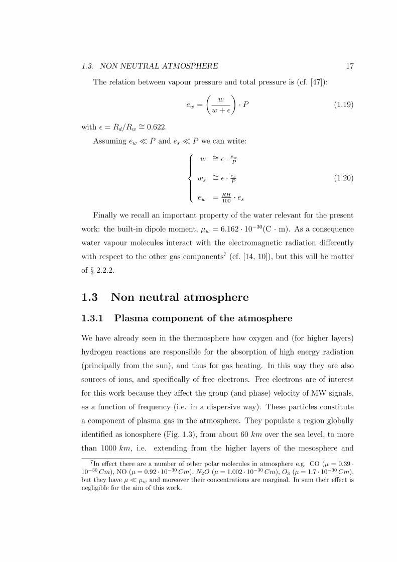
Air is a low efficient heat conductor (Fig. 1.5). This, and the lack of other
efficient mechanisms of heat transfer among gas parcels, allows to reasonably
assume that a moving gas parcel behaves adiabatically (cf. [18]):
T
Pγ−1γ
= cost. (1.10)
4Md =∑imi/
∑imiMi
, with mi and Mi, molecular mass and weight respectively, for the ith
gas specie of the dry mixture. For the dry atmosphere Md = 28.97 Kmol.
14 CHAPTER 1. STATIONARY VIEW OF THE EARTH ATMOSPHERE
with γ = CP/CV , ratio of specific heats at constant pressure and volume re-
spectively, for the gas mixture. Differentiating Eq. (1.10) and using Eq. (1.1)
and (1.2), we find:
T = T0 − Γd(z − z0) (1.11)
with T0 temperature at z0 and Γd = gRd
(γ−1γ
)adiabatic lapse rate.
From statistical mechanics we know that, for a biatomic gas, γ = 75
(cf. [49])
and Γd ∼= 9.8 K/km.
When condensing water vapour releases latent heat. A rising moist gas parcel,
with saturated water vapour, cools slower than a dry one, as, in saturation
conditions, a temperature reduction is accompanied by vapour condensation and
thus by heat release within the parcel. The adiabatic lapse rate for wet saturated
air is very variable, it strongly depends on temperature, thus, on average, it
depends on latitude too5
The following relationships thus give the standard temperature profile for dry
atmosphere in the troposphere (the one of main interest for this work):T (z) = T0 − Γs · z
T0 = 288.15 K
Γs = 6.5 K/km
(1.12)
Pressure is given by Eq. (1.1) and (1.8), assuming Eq. (1.12) for temperature:P (z) = P0
(T0T
)−αP0 = 1013.25 hPa
α = 5.25
(1.13)
The main sources of profile departures from this standard are due water
vapour and atmospheric horizontal and vertical dynamics, from large to local
scales, that generate the meteorological phenomena. Mass air advections, con-
vections and precipitations make the temperature values and lapse rate very
5See note 2.
1.2. NEUTRAL ATMOSPHERE 15
variable, conditioned by latitudes, annual and diurnal cycles, up to local char-
acteristics, such as orography, proximity of water basins, land coverage, etc.
Especially the lower tropospheric layers can exhibit temperature behaviour very
different from standard, including temporary lapse rate inversions. Pressure in-
stead shows relevant changes in local values but not in the profile trends.
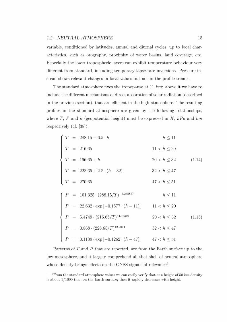
The standard atmosphere fixes the tropopause at 11 km: above it we have to
include the different mechanisms of direct absorption of solar radiation (described
in the previous section), that are efficient in the high atmosphere. The resulting
profiles in the standard atmosphere are given by the following relationships,
where T , P and h (geopotential height) must be expressed in K, kPa and km
respectively (cf. [38]):
T = 288.15− 6.5 · h h ≤ 11
T = 216.65 11 < h ≤ 20
T = 196.65 + h 20 < h ≤ 32
T = 228.65 + 2.8 · (h− 32) 32 < h ≤ 47
T = 270.65 47 < h ≤ 51
(1.14)
P = 101.325 · (288.15/T )−5.255877 h ≤ 11
P = 22.632 · exp [−0.1577 · (h− 11)] 11 < h ≤ 20
P = 5.4749 · (216.65/T )34.16319 20 < h ≤ 32
P = 0.868 · (228.65/T )12.2011 32 < h ≤ 47
P = 0.1109 · exp [−0.1262 · (h− 47)] 47 < h ≤ 51
(1.15)
Patterns of T and P that are reported, are from the Earth surface up to the
low mesosphere, and it largely comprehend all that shell of neutral atmosphere
whose density brings effects on the GNSS signals of relevance6.
6From the standard atmosphere values we can easily verify that at a height of 50 km densityis about 1/1000 than on the Earth surface; then it rapidly decreases with height.
16 CHAPTER 1. STATIONARY VIEW OF THE EARTH ATMOSPHERE
1.2.3 Water vapour distribution and laws
Water vapour is the main variable gas component of the atmosphere. Its presence
is essentially limited to the troposphere and in particular to the low tropospheric
layers. In fact it is part of the Earth water cycle, thus continuously released in
atmosphere by the Earth surface (from oceans, soil, vegetation, etc.) and then
removed as precipitation. Water vapour does not normally exceed a concentra-
tion of 4% in atmosphere (cf. [47]), but it is a main “ingredient” in meteorology
because of the importance of precipitation phenomena and of the absorption
and release of latent heat during the processes of evaporation and condensation
respectively, that condition the atmospheric dynamics (cf. [4]).
Water vapour can be modelled in the ideal gas approximation for a large
number of problems. The laws introduced for the dry atmosphere can conse-
quently applied to water vapour too, provided we use proper values for the gas
parameters: e.g. it holds the relationship:
ew = Rw ρ T (1.16)
with ew vapour partial pressure and Rw gas constant for water vapour.
The saturation pressure es can be obtained from the semi-empirical Buck law
(cf. [8]) (derived from the Clausius-Clapeyron law, cf. [18]):
es = A · 10aTcb+Tc (1.17)
with A = 6.11 hPa, a = 7.5 and b = 237.7, and being Tc the temperature
expressed in Celsius degrees.
Another parameter of common use is the relative humidity, RH, that ex-
presses the percentage of vapour, w, with respect to the saturation value, ws:
RH = 100w
ws(1.18)
w and ws are expressed in term of mass mixing ratio, that is w = mw/md
(commonly in g/kg).
1.3. NON NEUTRAL ATMOSPHERE 17
The relation between vapour pressure and total pressure is (cf. [47]):
ew =
(w
w + ε
)· P (1.19)
with ε = Rd/Rw∼= 0.622.
Assuming ew P and es P we can write:w ∼= ε · ew
P
ws ∼= ε · esP
ew = RH100· es
(1.20)
Finally we recall an important property of the water relevant for the present
work: the built-in dipole moment, µw = 6.162 · 10−30(C · m). As a consequence
water vapour molecules interact with the electromagnetic radiation differently
with respect to the other gas components7 (cf. [14, 10]), but this will be matter
of § 2.2.2.
1.3 Non neutral atmosphere
1.3.1 Plasma component of the atmosphere
We have already seen in the thermosphere how oxygen and (for higher layers)
hydrogen reactions are responsible for the absorption of high energy radiation
(principally from the sun), and thus for gas heating. In this way they are also
sources of ions, and specifically of free electrons. Free electrons are of interest
for this work because they affect the group (and phase) velocity of MW signals,
as a function of frequency (i.e. in a dispersive way). These particles constitute
a component of plasma gas in the atmosphere. They populate a region globally
identified as ionosphere (Fig. 1.3), from about 60 km over the sea level, to more
than 1000 km, i.e. extending from the higher layers of the mesosphere and
7In effect there are a number of other polar molecules in atmosphere e.g. CO (µ = 0.39 ·10−30 Cm), NO (µ = 0.92 · 10−30 Cm), N2O (µ = 1.002 · 10−30 Cm), O3 (µ = 1.7 · 10−30 Cm),but they have µ µw and moreover their concentrations are marginal. In sum their effect isnegligible for the aim of this work.
18 CHAPTER 1. STATIONARY VIEW OF THE EARTH ATMOSPHERE
including all the thermosphere, up to a large part of the exosphere, where it is
identified more specifically as protonosphere.
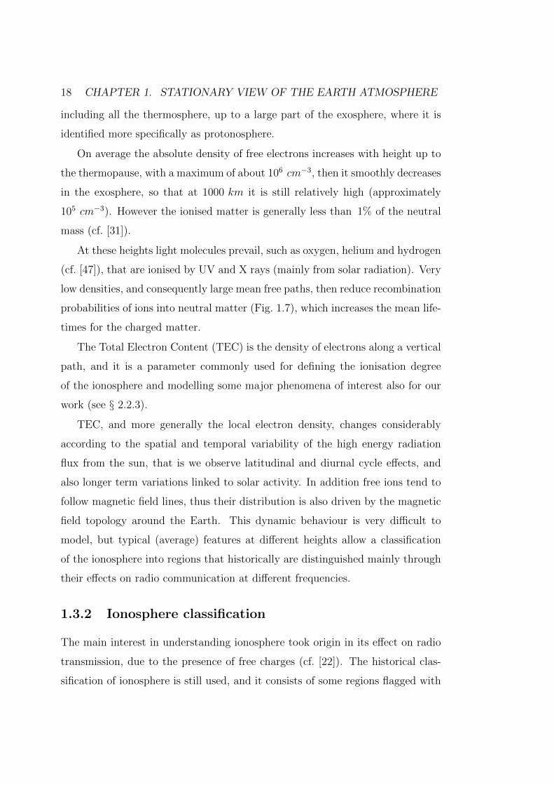
On average the absolute density of free electrons increases with height up to
the thermopause, with a maximum of about 106 cm−3, then it smoothly decreases
in the exosphere, so that at 1000 km it is still relatively high (approximately
105 cm−3). However the ionised matter is generally less than 1% of the neutral
mass (cf. [31]).
At these heights light molecules prevail, such as oxygen, helium and hydrogen
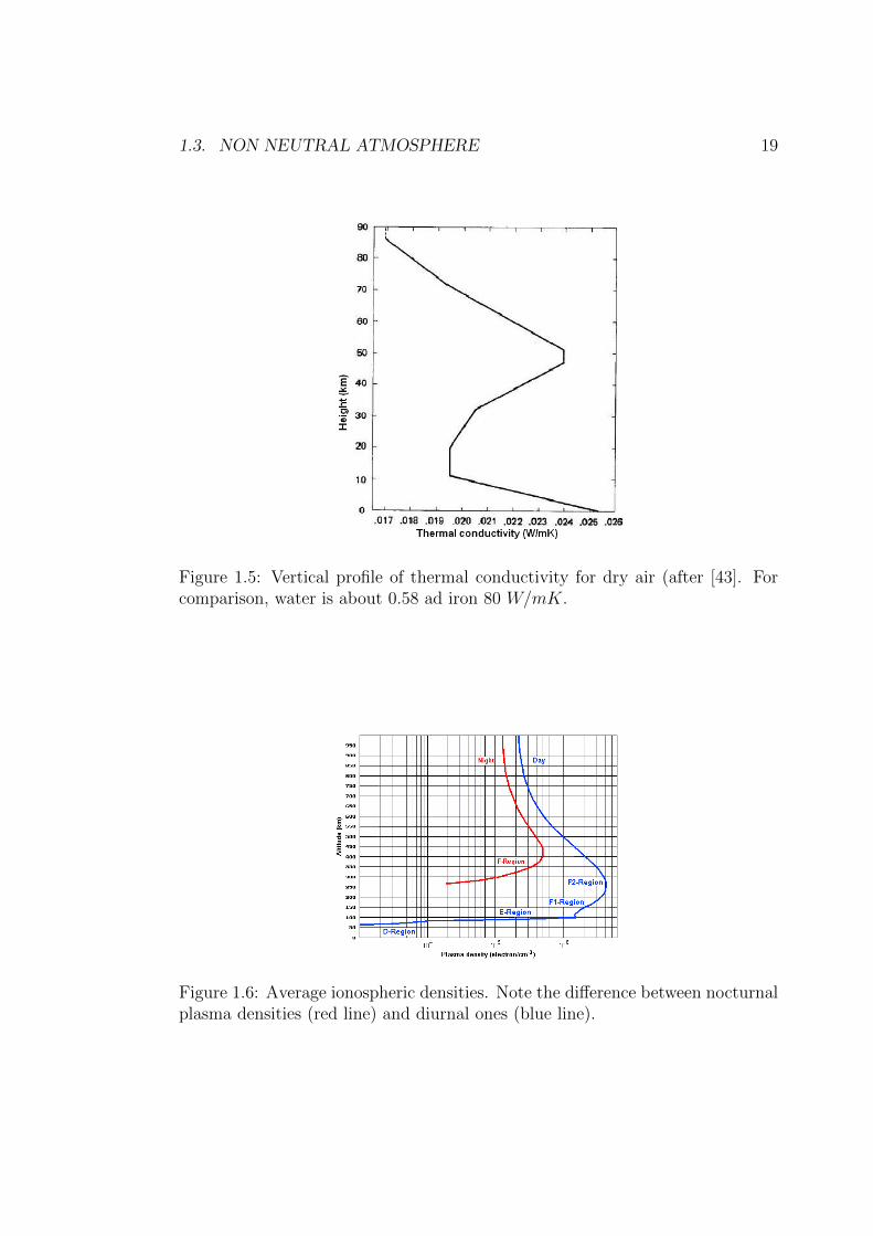
(cf. [47]), that are ionised by UV and X rays (mainly from solar radiation). Very
low densities, and consequently large mean free paths, then reduce recombination
probabilities of ions into neutral matter (Fig. 1.7), which increases the mean life-
times for the charged matter.
The Total Electron Content (TEC) is the density of electrons along a vertical
path, and it is a parameter commonly used for defining the ionisation degree
of the ionosphere and modelling some major phenomena of interest also for our
work (see § 2.2.3).
TEC, and more generally the local electron density, changes considerably
according to the spatial and temporal variability of the high energy radiation
flux from the sun, that is we observe latitudinal and diurnal cycle effects, and
also longer term variations linked to solar activity. In addition free ions tend to
follow magnetic field lines, thus their distribution is also driven by the magnetic
field topology around the Earth. This dynamic behaviour is very difficult to
model, but typical (average) features at different heights allow a classification
of the ionosphere into regions that historically are distinguished mainly through
their effects on radio communication at different frequencies.
1.3.2 Ionosphere classification
The main interest in understanding ionosphere took origin in its effect on radio
transmission, due to the presence of free charges (cf. [22]). The historical clas-
sification of ionosphere is still used, and it consists of some regions flagged with
1.3. NON NEUTRAL ATMOSPHERE 19
Figure 1.5: Vertical profile of thermal conductivity for dry air (after [43]. Forcomparison, water is about 0.58 ad iron 80 W/mK.
Figure 1.6: Average ionospheric densities. Note the difference between nocturnalplasma densities (red line) and diurnal ones (blue line).
20 CHAPTER 1. STATIONARY VIEW OF THE EARTH ATMOSPHERE
Figure 1.7: Mean free path of particles in atmosphere (after [43]).
alphabetic letters.
D is the lowest region, located between 75 and 95 km, and it is responsible
for the propagation of radio signals at frequencies ≤ 2MHz. This layer exists
only during daytime, as at this height the density makes the recombination
processes effective enough to neutralise the charged matter during night, when
the ionisation engine is off.
E is the second region located between 95 and 150 km, and exists also during
the night (due to the reduced efficiency of the recombination processes). O2+ are
the principal ions of this region, that allow signal transmission up to 10MHz.
F is the third region located from 150 to about 500 km. O+ and also NO+ are
the prevalent ions, and, also due to its large extension (that increases during the
daytime), is the most important region for high frequency radio transmission.
1.3. NON NEUTRAL ATMOSPHERE 21
The topside region is the last region extending over the F region, which is
composed mainly by H+ ions. Low particle density however makes this region
less relevant in radio transmission phenomena.
22 CHAPTER 1. STATIONARY VIEW OF THE EARTH ATMOSPHERE
Chapter 2
Atmospheric effects on GNSSsignals
2.1 Propagating electromagnetic signals
A GNSS signal is an electromagnetic wave packet with a carrier frequency at L
band, i.e. between 1 and 2 GHz (according to the GNSS constellation and signal
type), travelling from the satellite towards the Earth, where receivers decode and
process it. Such signal comes from an essentially vacuum environment around
the satellite, then crosses the rarefied but ionised gas of the high atmosphere
(i.e. the ionosphere), and finally the low atmosphere, which is neutral but whose
density brings non negligible effects on radiation, due to both the dry component
and the water vapour, in different ways.
The aim of this chapter is to summarise the basic processes that affect an
electromagnetic signal travelling in a medium like the atmosphere, in order to
introduce the equations and the built-in approximations we will refer to, when
dealing with ionospheric free GNSS signals. Such equations have been imple-
mented in a simulator of GNSS signals travelling in the atmosphere, that has
been built to implement the core part of the whole thesis, i.e. the tests on the
algorithms for retrieving tropospheric profiles from GPS-like signals.
An electromagnetic wave in the vacuum comes as solution of the Maxwell
equations for each component of the electric and magnetic field vectors, E and
23
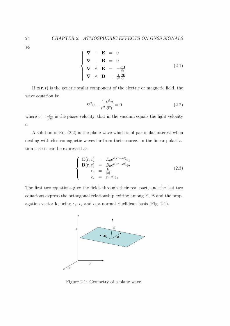
24 CHAPTER 2. ATMOSPHERIC EFFECTS ON GNSS SIGNALS
B:
∇ · E = 0
∇ · B = 0
∇ ∧ E = −∂B∂t
∇ ∧ B = 1c2∂E∂t
(2.1)
If u(r, t) is the generic scalar component of the electric or magnetic field, the
wave equation is:
∇2u− 1
v2
∂2u
∂2t= 0 (2.2)
where v = c√µε
is the phase velocity, that in the vacuum equals the light velocity
c.
A solution of Eq. (2.2) is the plane wave which is of particular interest when
dealing with electromagnetic waves far from their source. In the linear polarisa-
tion case it can be expressed as:E(r, t) = E0e
i(kr−ωt)ε1B(r, t) = B0e
i(kr−ωt)ε2ε3 = k
|k|ε2 = ε3 ∧ ε1
(2.3)
The first two equations give the fields through their real part, and the last two
equations express the orthogonal relationship exiting among E, B and the prop-
agation vector k, being ε1, ε2 and ε3 a normal Euclidean basis (Fig. 2.1).
Figure 2.1: Geometry of a plane wave.
2.2. ELECTROMAGNETIC SIGNALS IN GAS MEDIA 25
What we have written for a single wave frequency (i.e. in the ideal monochro-
matic case) can be straightforwardly generalised to generic wave packets, as real
electromagnetic signals are, following the Fourier theorem, a linear combination
of an infinite number of monochromatic waves, with given amplitude and phase
(cf. [22]).
In the following sections we will address the issue of what happens to local
fields when an electromagnetic wave propagates through a gas medium.
2.2 Electromagnetic signals in gas media
An electromagnetic wave propagates the E and B vector fields: in a given point
this means we have time-varying fields. A gas particle interacts with these fields,
both if it is neutral and furthermore if it is polarised or ionised, and due to this
interaction the fields partially change.
A rigorous analysis of these phenomena would need a complex quantum me-
chanical approach, that is out of the scope of the present work. Nevertheless,
the interaction can be modeled using a classical approach with results (at least
qualitatively) coherent with the semi-empirical approach of wide use, based on
the geometrical optics approximation and on experimental findings. However
our approach will permit also to explicitly quantify the magnitude of some ap-
proximations that are included in the semi-empirical approach.
2.2.1 Interaction with a neutral non-polarised gas
The neutral non polarised part of the atmospheric gases is essentially what is
called dry atmosphere, which is mainly concentrated in the troposphere and low
stratosphere.
An electromagnetic wave interacts with neutral atoms or molecules through
the mechanisms of excitation of the particle energy levels, responsible for ab-
sorption and (spontaneous plus stimulated) emission phenomena. As a conse-
quence an electromagnetic wave crossing a gas layer will be generally subjected
26 CHAPTER 2. ATMOSPHERIC EFFECTS ON GNSS SIGNALS
to changes in intensity and phase.
A very rough but still useful description of the phenomena can be obtained by
a simple classical representation of each gas particle as a negative charged cloud
due to electron(s), surrounding a positive charged nucleus, both having spherical
shapes with coincident centres. In this simplified view the presence of an electric
field E induces a cloud deformation, and consequently the displacement of the
negative cloud centre from the positive nucleus one. Such displacement in turn
produces a restoring electric force, between the two centres.
Figure 2.2: Simplified classical view of charge displacement in an atom immersedin an electric field.
We can make the following assumptions that are more than reasonable in
many cases, including the one of interest for this work:
1. the displacement is instantaneous with respect to E variations (i.e. electron
inertia is negligible with respect to the wave period);
2. the effect of B on this phenomenon is negligible;
3. the electron cloud displacement is much less than the cloud dimension (i.e.
the intensity of E so low that induces just a perturbation in the particle
charge symmetry).
In these hypotheses our problems reduces to the study of an harmonic oscil-
lator forced by an electric force, periodic with time. In fact from item 2 we can
neglect B; item 1 says that E and the charge cloud move in phase, and it is easy
2.2. ELECTROMAGNETIC SIGNALS IN GAS MEDIA 27
to demonstrate that item 3 leads to a restoring force f that is elastic. In fact
the charge responsible for the restoring force is only the one inside the sphere of
radius x in Fig. 2.2, and thus we have1:
f ' − Zq
4πε0·ρq(
4π3
)x3
x2· xx
(2.4)
with x cloud displacement vector of module x; q proton charge; Z atomic num-
ber of the gas particle; ρq mean charge density of the electron cloud roughly
equivalent to Zq
( 43πa3)
with a mean particle radius. At the end we find f ∝ x that
reduces the problem to the oscillator one:
x(t) + ω20x(t) =
q E
m(2.5)
being ω0 =√
Z2q24π3ma3
the oscillator own frequency, with m mass of the electron
cloud, and E forcing field.
In the ideal oscillator case if f varies periodically with a frequency close
to the resonant one (i.e. ω0), the amplitude of the periodic solutions tends
to diverge to infinity. In real cases (e.g. in mechanical oscillator) for large
amplitudes the oscillator does no more behave as an harmonic one. Normally
a damping term is added to the oscillator equation, that accounts for inelastic
phenomena, dissipating the energy acquired (in excess) by the forcing term. The
quantum counterpart of such inelastic interactions are the radiation absorption
and stimulated emission that happen in real atoms (or molecules) when radiation
frequencies are close to the resonant atomic (or molecular) frequencies. In our
still simplified view we can write:
x(t) + 2γx(t) + ω20x(t) =
−qmE0e
iω[t− zc
] (2.6)
On the left side of the equation we have explicitly included the forcing term, or
more correctly one of its Fourier component, with the time phase delay due to
the distance z of the gas particle from the radiation source (being c the speed of
1The charge outside such sphere gives a null total contribution to f , thanks to the Gausstheorem.
28 CHAPTER 2. ATMOSPHERIC EFFECTS ON GNSS SIGNALS
light in the vacuum). The solution is:
x(t) =qE0 e
iω[t− zc
]
A(ω, ω0, γ)(2.7)
with:
A(ω, ω0, γ) = m(ω2 − ω20 − 2iγω) (2.8)
GNSS systems have been designed in order to avoid problems of signal amplitude
reductions, thus their operational frequencies are far from the absorption lines
of atmospheric molecules (i.e. |ω − ω0| 0). In other words we could neglect
the term with γ and simplify Eq. (2.7) with A ' m(ω2 − ω20).
Previous equation says that our neutral and non polarised gas particle be-
comes an oscillating dipole when “forced” by an electromagnetic radiation, with
momentum P(r, t) proportional to the incident electric filed. Thus it becomes in
turn a source of electromagnetic radiation, according to the following equations
(cf. [19]). E(r, t) = − q
4πε0
[er′r′2
+ r′
cddt
(er′r′2
)+ 1
c2d2
dt2er′
]B = e′r×Er
c
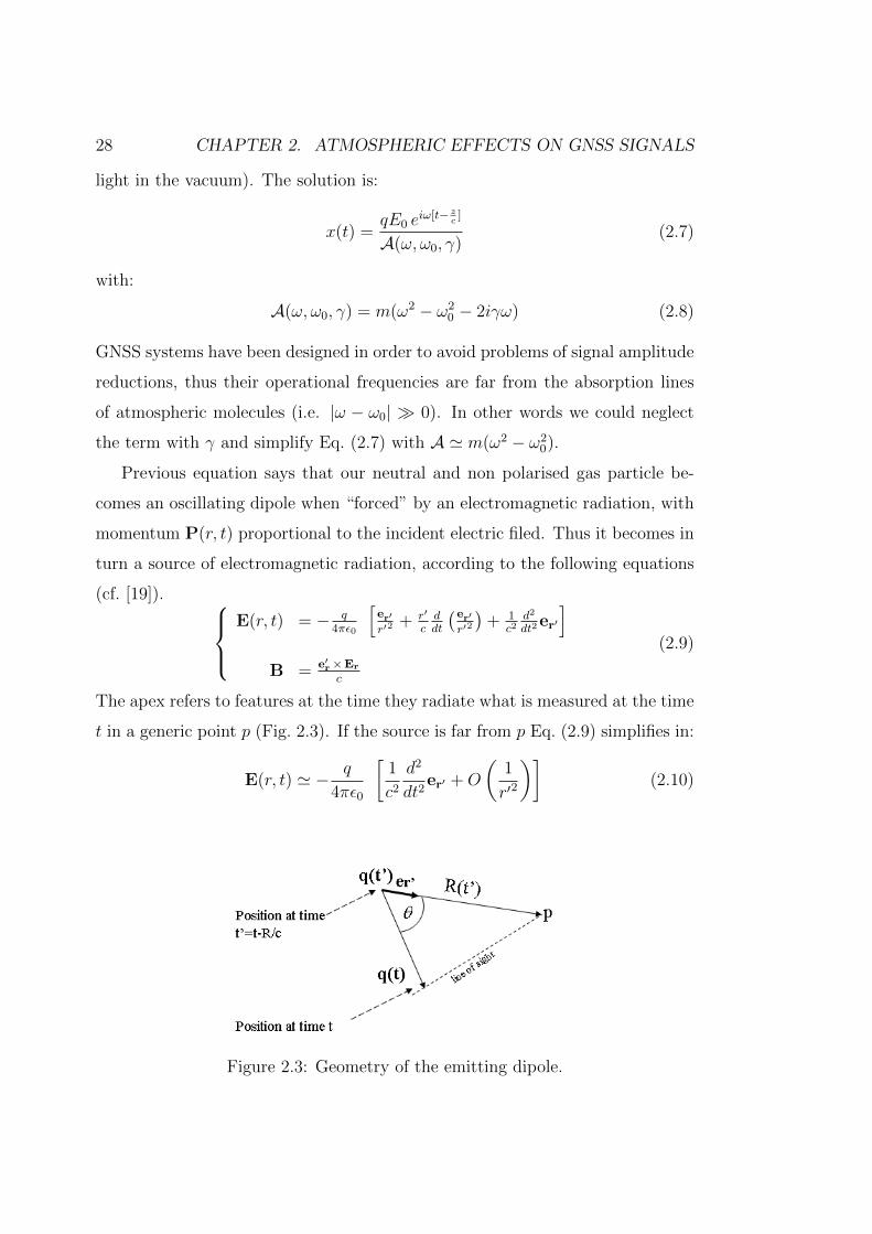
(2.9)
The apex refers to features at the time they radiate what is measured at the time
t in a generic point p (Fig. 2.3). If the source is far from p Eq. (2.9) simplifies in:
E(r, t) ' − q
4πε0
[1
c2
d2
dt2er′ +O
(1
r′2
)](2.10)
Figure 2.3: Geometry of the emitting dipole.
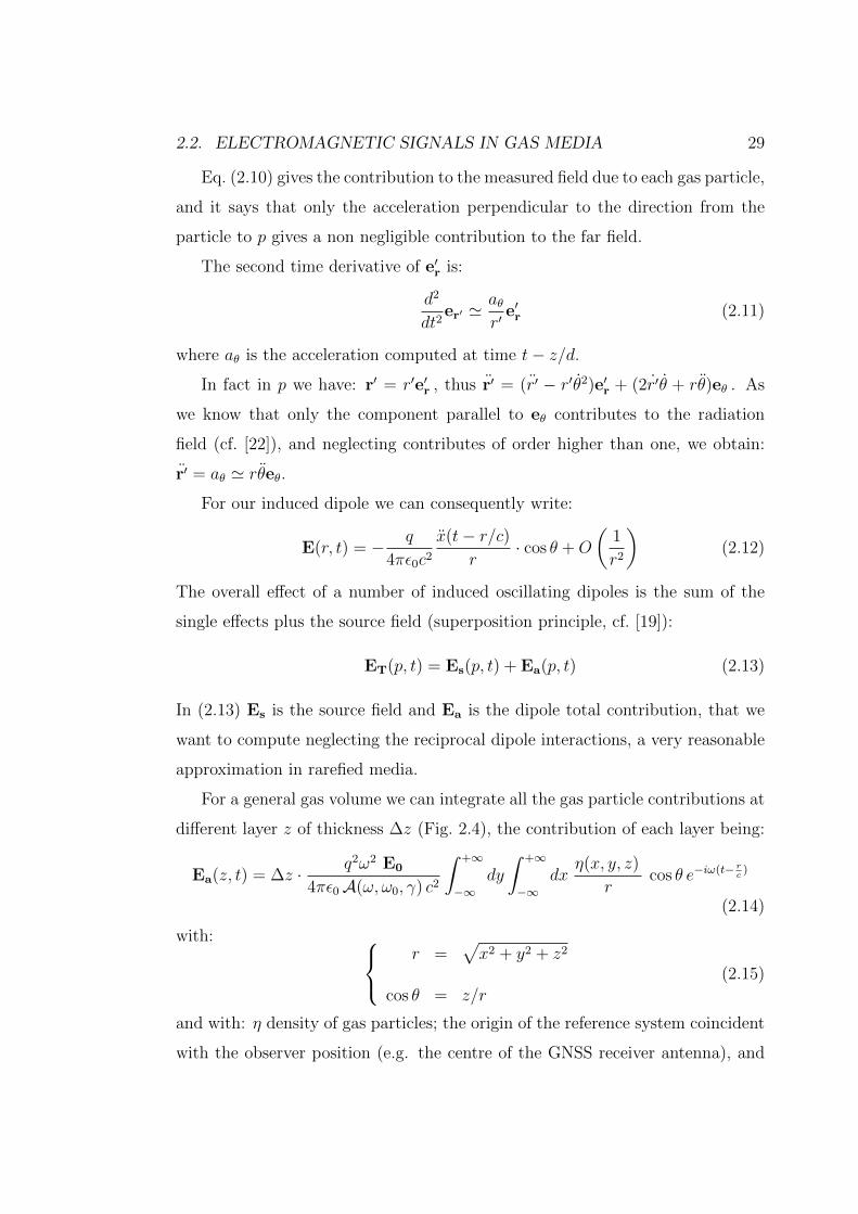
2.2. ELECTROMAGNETIC SIGNALS IN GAS MEDIA 29
Eq. (2.10) gives the contribution to the measured field due to each gas particle,
and it says that only the acceleration perpendicular to the direction from the
particle to p gives a non negligible contribution to the far field.
The second time derivative of e′r is:
d2
dt2er′ '
aθr′
e′r (2.11)
where aθ is the acceleration computed at time t− z/d.
In fact in p we have: r′ = r′e′r , thus r′ = (r′ − r′θ2)e′r + (2r′θ + rθ)eθ . As
we know that only the component parallel to eθ contributes to the radiation
field (cf. [22]), and neglecting contributes of order higher than one, we obtain:
r′ = aθ ' rθeθ.
For our induced dipole we can consequently write:
E(r, t) = − q
4πε0c2
x(t− r/c)r
· cos θ +O
(1
r2
)(2.12)
The overall effect of a number of induced oscillating dipoles is the sum of the
single effects plus the source field (superposition principle, cf. [19]):
ET(p, t) = Es(p, t) + Ea(p, t) (2.13)
In (2.13) Es is the source field and Ea is the dipole total contribution, that we
want to compute neglecting the reciprocal dipole interactions, a very reasonable
approximation in rarefied media.
For a general gas volume we can integrate all the gas particle contributions at
different layer z of thickness ∆z (Fig. 2.4), the contribution of each layer being:
Ea(z, t) = ∆z · q2ω2 E0
4πε0A(ω, ω0, γ) c2
∫ +∞
−∞dy
∫ +∞
−∞dx
η(x, y, z)
rcos θ e−iω(t− r
c)
(2.14)
with: r =√x2 + y2 + z2
cos θ = z/r
(2.15)
and with: η density of gas particles; the origin of the reference system coincident
with the observer position (e.g. the centre of the GNSS receiver antenna), and
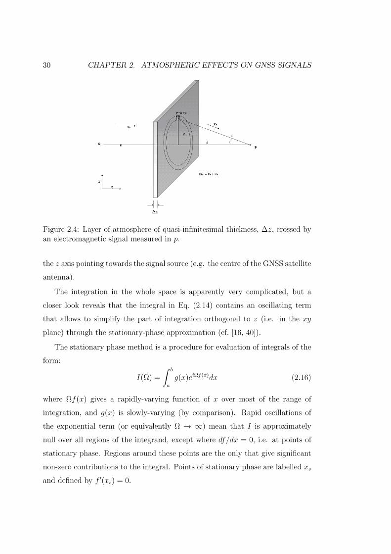
30 CHAPTER 2. ATMOSPHERIC EFFECTS ON GNSS SIGNALS
Figure 2.4: Layer of atmosphere of quasi-infinitesimal thickness, ∆z, crossed byan electromagnetic signal measured in p.
the z axis pointing towards the signal source (e.g. the centre of the GNSS satellite
antenna).
The integration in the whole space is apparently very complicated, but a
closer look reveals that the integral in Eq. (2.14) contains an oscillating term
that allows to simplify the part of integration orthogonal to z (i.e. in the xy
plane) through the stationary-phase approximation (cf. [16, 40]).
The stationary phase method is a procedure for evaluation of integrals of the
form:
I(Ω) =
∫ b
a
g(x)eiΩf(x)dx (2.16)
where Ωf(x) gives a rapidly-varying function of x over most of the range of
integration, and g(x) is slowly-varying (by comparison). Rapid oscillations of
the exponential term (or equivalently Ω → ∞) mean that I is approximately
null over all regions of the integrand, except where df/dx = 0, i.e. at points of
stationary phase. Regions around these points are the only that give significant
non-zero contributions to the integral. Points of stationary phase are labelled xs
and defined by f ′(xs) = 0.
2.2. ELECTROMAGNETIC SIGNALS IN GAS MEDIA 31
In the vicinity of the stationary phase points we have g(x) ' g(xs), since we
remind that g(x) is assumed to be slowly varying, and hence this term can be
pulled outside the integral.
Expanding f(x) in a Taylor series near xs up to the second order and assuming
f ′′(xs) 6= 0, we have:
f(x) ' f(xs) +1
2f ′′(xs)(x− xs)2 (2.17)
Substituting this into Eq. (2.16) we obtain:
I(Ω) =1√Ω·
[√2πi
f ′′(xs)g(xs) e
iΩf(xs)
]+O(
1
Ω) (2.18)
For integrals in two dimensions, we essentially proceed in the same way, and the
result is:
I(Ω) =1
Ω·
2πi · g(xs, ys) eiΩf(xs,ys)√
fxx(xs, ys) · fyy(xs, ys)− f 2xy(xs, ys)
+O(1
Ω2) (2.19)
The integral of Eq. (2.14) becomes something that depends no more on the
whole gas volume, but only on a cylinder of (variable) section S equal to:
S = Ω ·(√
fxxfyy − f 2xy
)∣∣∣(xs,ys)
(2.20)
This can be imagined as a sort of tube whose axis is on the stationary phase
points. If the section is small we can approximate the tube with a line, in other
words we can proceed in the geometrical optics approximation. In our problem
“small” is what is less than the spatial resolution sought for our tropospheric
parameters.
If η depends only on z it can be pulled outside the integrals in dx and dy,
and we easily find that the ray path stays on the z axis. On the contrary if η has
a gradient orthogonal to z that cannot be neglected with respect to the integral
oscillating term, the stationary phase approximation needs to account for more
terms than what we have done, and one of the differences in the final result is
32 CHAPTER 2. ATMOSPHERIC EFFECTS ON GNSS SIGNALS
that the ray path departs from a straight line, showing a bending, problem that
we will address later in § 2.3.2.
For the moment if we assume our approximations as reasonable, from Eq. (2.14)
and Eq. (2.15) we can write: g(x, y) = η/r2
f(x, y) = −rΩ = ω/c
(2.21)
For the derivatives of f we have:fx = −x/rfy = −y/rfxx = −(r2 − x2)/r3
fyy = −(r2 − y2)/r3
fxy = fyx = −(xy)/r3
(2.22)
Stationary points are consequently in (x, y) = (0, 0) ∀z and they imply:fxx = fyy = −1/zfxy = fyx = 0
(2.23)
Eq. (2.14) becomes:
Ea(z, t) = ∆z · iΩ2ε0
q2
A(ω, ω0, γ)η(0, 0, z)E0 e
−iω(t− zc
) (2.24)
From Eq. (2.13) and Eq. (2.24) we have also:
ET(p, t) = Es(p, t)
(1 + ∆z · iΩ
2ε0
q2
A(ω, ω0, γ)η(0, 0, z)
)(2.25)
It can be compared with the equations valid in the geometrical optics approxi-
mation for electromagnetic waves in non vacuum (but non ferromagnetic) media.
Specifically the phase delay due to a medium of thickness ∆z and refractive index
n, is:
ET(p, t) = Es(p, t) eiφt (2.26)
with φ = ωc(n − 1)∆z. Comparing the two equations for ∆z → 0 we obtain a
relationship between the macroscopic properties of the medium and the refractive
index:
n = 1 +iΩ
2ε0
q2
A(ω, ω0, γ)η(0, 0, z) (2.27)
2.2. ELECTROMAGNETIC SIGNALS IN GAS MEDIA 33
Generally n is a complex number. Its imaginary part comes from the γ term
in A(ω, ω0, γ), and it reduces the module of the field, thus the amplitude of the
wave. We have already commented that this aspect is negligible in our problem.
The real part of n instead can be interpreted as a term n = c/v, thus a change
in the propagation velocity of the wave from c, in the vacuum, to v, in the (gas)
medium, and consequently in the travel time of the wave packet: this is the
property at the basis of atmospheric sounding by means of GNSS signals.
From our derivation we find n = n(ω0, γ, ω, η) and specifically n ∝ η. It
means that n depends on the gas composition, through the atoms properties
contained in ω0 and γ, on the incident radiation through ω and on the local
thermodynamic properties through η.
In real atoms and molecules the resonant frequencies are much more than
one; they are related to emission/absorption lines and they are given by quan-
tum mechanics. In the troposphere, non polar molecules typically have major
resonant lines around the visible or near infrared frequencies (∼ 1015Hz): if we
assume η(z) = 1kB
PT
, we find n ' 1.00016.
From this point of view the classical approach we derived from Eq. (2.24)
gives a good order of magnitude for n, whose typical values are about 1.0002.
It is however too simplified to allow a precise quantitative computation of n.
Other approaches still quasi-classical as the Lorentz and Debye ones (cf. [14, 45])
are necessary at this purpose. Nevertheless the linear dependence of n on η
we have derived, finds experimental confirmations, and essentially this is what
will be used in this work. In addition, the derivation we have performed is
meaningful for evaluating the approximations included in the geometrical optics
assumptions. In particular geometrical optics reduces a 3D problem to a 1D
one, but Eq. (2.19) and Eq. (2.24) say that the 1D approximation along the ray
path direction z, implies averaging the medium parameters on xy surfaces of
finite dimension, that at GNSS frequencies are about 0.2 z m2, for z measured
in meters. This poses a theoretical limit to the possibility of resolving horizontal
atmospheric structures, that at the top of the troposphere is around 50 m.
34 CHAPTER 2. ATMOSPHERIC EFFECTS ON GNSS SIGNALS
In the atmosphere we can assume valid the ideal gas approximation, thus we
have η ∝ P/T and as a consequence, for a neutral non polarised gas, we find
n ∝ P/T . There are other two relevant properties of n in the troposphere (and
stratosphere too) specifically related to radiation at GNSS frequencies:
1. n is real (i.e. the imaginary part is essentially negligible);
2. n does not depend on the radiation frequency.
If we want to explain these properties still through a quasi-classical scheme, we
can say that ω is so far from the resonant frequencies that in n the contribution
of the γ damping term vanishes, and n is such that dn/dω ' 0. In other words
the neutral atmosphere at GNSS frequencies is essentially not absorbing and non
dispersive.
Precise values of n for the neutral atmosphere have been assessed through ex-
perimental works. In the present work an empirical relationship is used (cf. [39])
that associates n to the atmospheric state variables:
n = 1 + c1PdT
(2.28)
with c1 = 10−6 · (77.604 ± 0.014)K/mb. A more refined expression is given by
the same authors accounting for non ideal-gas behaviours:
n = 1 + c1PdT· (Zd)−1 (2.29)
where Zd is a compressibility coefficient for the real atmospheric gas mixture
defined as:
(Zd)−1 = 1 + Pd[57.97 · 10−8(1 + 0.52/T )− 9.4611 · 10−4Tc/T
2] (2.30)
with Tc given in Celsius degrees.
2.2.2 Interaction with a neutral but polarised gas
.
2.2. ELECTROMAGNETIC SIGNALS IN GAS MEDIA 35
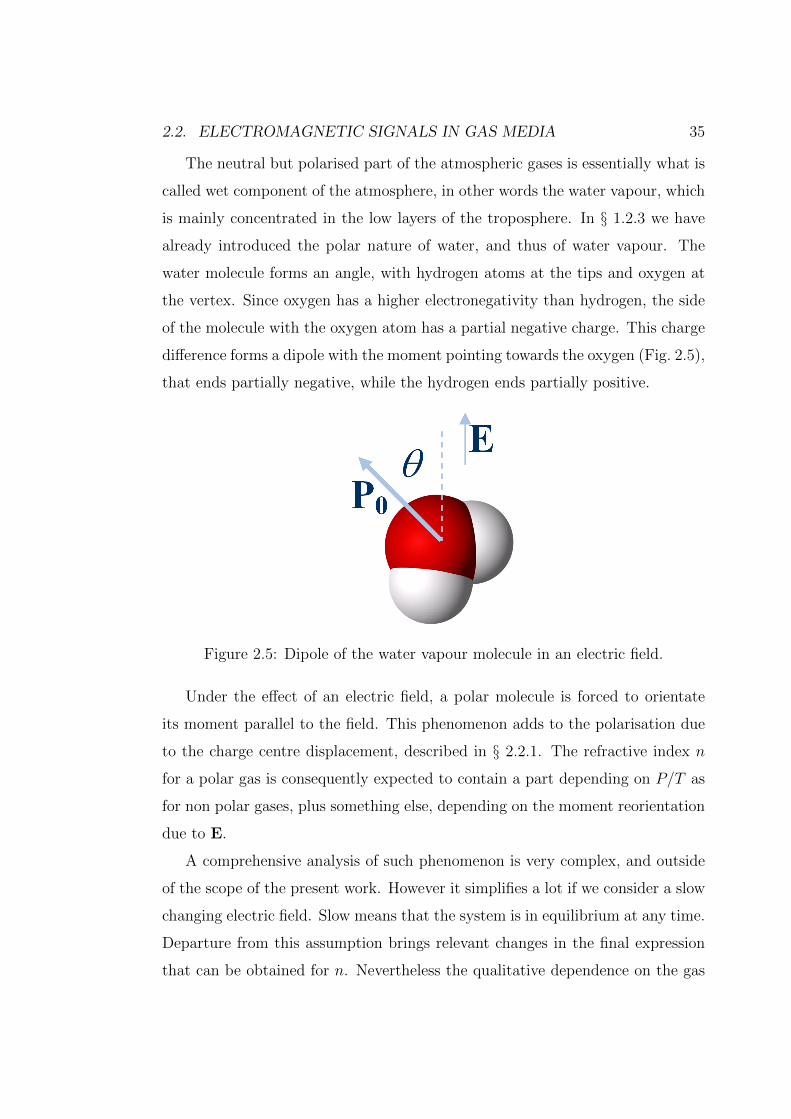
The neutral but polarised part of the atmospheric gases is essentially what is
called wet component of the atmosphere, in other words the water vapour, which
is mainly concentrated in the low layers of the troposphere. In § 1.2.3 we have
already introduced the polar nature of water, and thus of water vapour. The
water molecule forms an angle, with hydrogen atoms at the tips and oxygen at
the vertex. Since oxygen has a higher electronegativity than hydrogen, the side
of the molecule with the oxygen atom has a partial negative charge. This charge
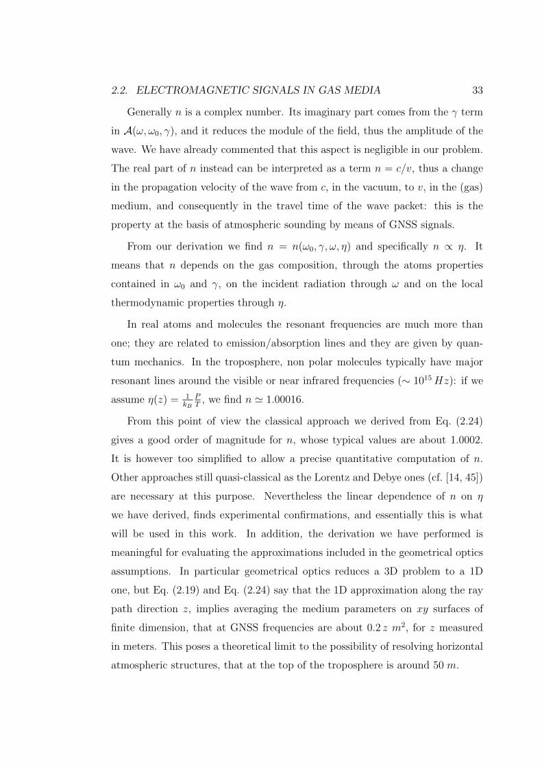
difference forms a dipole with the moment pointing towards the oxygen (Fig. 2.5),
that ends partially negative, while the hydrogen ends partially positive.
Figure 2.5: Dipole of the water vapour molecule in an electric field.
Under the effect of an electric field, a polar molecule is forced to orientate
its moment parallel to the field. This phenomenon adds to the polarisation due
to the charge centre displacement, described in § 2.2.1. The refractive index n
for a polar gas is consequently expected to contain a part depending on P/T as
for non polar gases, plus something else, depending on the moment reorientation
due to E.
A comprehensive analysis of such phenomenon is very complex, and outside
of the scope of the present work. However it simplifies a lot if we consider a slow
changing electric field. Slow means that the system is in equilibrium at any time.
Departure from this assumption brings relevant changes in the final expression
that can be obtained for n. Nevertheless the qualitative dependence on the gas
36 CHAPTER 2. ATMOSPHERIC EFFECTS ON GNSS SIGNALS
parameters remains explained even with this strong hypothesis, while for the
final expression of n we will refer once again to experimental measurements.
If we immerse a gas of particles owing an electric moment p0 in an electric
field E, each particle will experiment a mechanical moment ~M as:
~M = p0 ∧ E (2.31)
that tends to align the particle electric moment parallel to the field, against
thermal energy that tends to randomise particle motions and thus orientations.
After a time interval τ (we suppose infinitesimal) we will reach an equilibrium
between these forcing terms. At the equilibrium the spatial distribution of p0
will form an average angle θ (see Fig. 2.5) such as we could write:
p = p0 cos θ (2.32)
where p0 = ‖p0‖ and overlined quantities are averaged on small gas volumes but
containing a large number of particles (in thermodynamic equilibrium). Namely
p is the module of the electric moment of the small gas volume, computed as the
mean of the single molecular electric moment vectors.
We can imagine θ satisfying the following generic limits:
limT→0
cos θ = limE→∞
cos θ = 1 (2.33)
limT→∞
cos θ = limE→0
cos θ = 0 (2.34)
In other words we expect to have all particles oriented as E when the thermal
motions becomes negligible with respect to the forcing effect due to the electric
field, that is for temperatures T (expressed in K) approaching to 0 or very in-
tense E. The opposite happens when the thermal motions dominate, bringing a
perfect stochastic orientation of p0, i.e. for very high T or negligible E. Ther-
modynamics gives a way to solve the dependence of cos θ on T and E. In fact
at the equilibrium we know that the number of particles with potential energy
E is distributed proportional to exp(−E/kT ), wth k Boltzmann constant. The
potential energy of the dipole is:
E = −p0 · E = −p0E cos θ (2.35)
2.2. ELECTROMAGNETIC SIGNALS IN GAS MEDIA 37
As a consequence the probability for θ will be:
P(θ) ∝ ep0EkT cos θ (2.36)
and thus:
cos θ =
∫ ∫cos θ P(θ) sin θ dθ dφ∫ ∫P(θ) sin θ dθ dφ
(2.37)
where the integration must be made over all directions, with 0 ≤ φ < 2π and
0 ≤ θ < π. Solving Eq. (2.37) we obtain the Langevin function, L(a):
cos θ = L(a) =ea + e−a
ea − e−a− 1
2= coth a− 1
2(2.38)
being a = p0EkT
.
For very small values of a, as in our case, namely for 0 < a 1, L(a) can
be developed and at the first order we have L(a) ' a/3. Thus Eq. (2.38) finally
gives:
p = p0cos θ = p0L(a) ' p20
3kTE (2.39)
Eq. (2.39) says that our gas particles behaves as having a dipole moment on
average proportional to the inverse of temperature, in addition to the induced
dipole moment as for the non polarised particles. What was done to obtain an
expression for n for neutral non polarised particles can be applied to the dipole
expression of Eq. (2.39). Thus for neutral and polarised ideal gases (whose
density is proportional to P/T ) we expect to have:
n = 1 +
induced polarisation︷ ︸︸ ︷A · P
T+
polarisation due to orientation︷ ︸︸ ︷B · P
T 2(2.40)
Of course, Eq. (2.40) holds also for non polarised gases; in this case we have
B = 0. More generally, for a mixture of neutral gases, we will have:
n = 1 +∑m
Am ·PmT
+∑p
(Ap +
BpT
)· PpT
(2.41)
where the index m maps specific constants and partial pressures for the neutral
gases and p for the polarised ones.
38 CHAPTER 2. ATMOSPHERIC EFFECTS ON GNSS SIGNALS
We have to stress that our derivation on how n depends on gas thermody-
namic parameters is just valid on a qualitative point of view (thus we will not re-
port quantification of n based on our modelling of polarised gases). Assumptions
made for a polarised gas in an electric field are stronger than what done for the
non polarised one. In fact our derivation assumed static E or eventually varying
E but as slowly as necessary to have a negligible time lag for the dipole reorien-
tation (i.e. instantaneous dipole reorientation). For electromagnetic waves thus
we should expect to find in n, namely in the Bp coefficients, some dependencies
on the wave frequency and on the molecule inertia. A complete analysis of the
problem, even through a quasi-classical approach (see for instance [45]), would
be too wide for the aim of the present work. In addition it is not necessary, as
we will refer to sound experimental results (c.f. [39]), whose precisions is about
0.02% (cf. [13]), that for a generic atmospheric gas composition (including water
vapour) give:
n = 1 + c1PdT· (Zd)−1 +
[c2 · (Zd)−1 +
c3
T· (Zw)−1
] eT
(2.42)
with Pd = P − e, dry pressure, being P the total pressure and e the partial
pressure of water vapour2. Constants are:c1 = 10−6 · (77.604± 0.014)K/mbc2 = 10−6 · (64.79± 0.08)K/mbc3 = 10−6 · (3776000± 4000)K2/mb
(2.43)
Finally the compressibility coefficients (to account for non ideal behaviours of
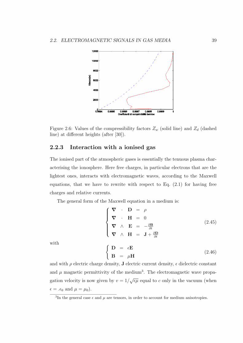
atmospheric gases) are the following, even if they give very fine corrections of a
few parts per thousands (see Fig. 2.6), that are not so relevant for the aim of our
work.(Zd)
−1 = 1 + Pd[57.97 · 10−8(1 + 0.52/T )− 9.4611 · 10−4Tc/T2]
(Zw)−1 = 1 + 1650(e/T 3)[1− 0.01317Tc + 1.75 · 10−4Tc2 + 1.44 · 10−6Tc
3]
(2.44)
Tc is the temperature expressed in Celsius degrees.
2In § 1 we have used ew for the water vapour pressure because of non-ambiguity reasons.In the following however we won’t have such problem, so we will used simply e for the partialpressure of water vapour.
2.2. ELECTROMAGNETIC SIGNALS IN GAS MEDIA 39
Figure 2.6: Values of the compressibility factors Zw (solid line) and Zd (dashedline) at different heights (after [30]).
2.2.3 Interaction with a ionised gas
The ionised part of the atmospheric gases is essentially the tenuous plasma char-
acterising the ionosphere. Here free charges, in particular electrons that are the
lightest ones, interacts with electromagnetic waves, according to the Maxwell
equations, that we have to rewrite with respect to Eq. (2.1) for having free
charges and relative currents.
The general form of the Maxwell equation in a medium is:∇ · D = ρ
∇ · H = 0
∇ ∧ E = −∂B∂t
∇ ∧ H = J + ∂D∂t
(2.45)
with D = εE
B = µH(2.46)
and with ρ electric charge density, J electric current density, ε dielectric constant
and µ magnetic permittivity of the medium3. The electromagnetic wave propa-
gation velocity is now given by v = 1/√εµ equal to c only in the vacuum (when
ε = .ε0 and µ = µ0).
3In the general case ε and µ are tensors, in order to account for medium anisotropies.
40 CHAPTER 2. ATMOSPHERIC EFFECTS ON GNSS SIGNALS
Eq. (2.45) and (2.45) allow to treat electromagnetic field propagation in a
medium knowing its macroscopic quantities. What we want to do is to anal-
yse the problem also from a point of view closer to the medium microscopic
properties.
The ionosphere is a very rarefied gas, whose major part is neutral and non
polar, giving a negligible effect on GNSS signals, according to Eq. (2.29). On the
contrary the effects of the charged part are to be quantified. Thus, for our scopes,
we can approximate ionosphere as an extremely rarefied gas of charged particles,
with a local charge balance between positive ions and electrons (i.e. ρ = 0), and
also thermodynamic equilibrium among charged particle populations (i.e. with
a unique defined temperature)4.
Eq. (2.45) consequently simplifies in:∇ · E = 0
∇ · µH = 0
∇ ∧ E = −∂B∂t
∇ ∧ H = σE + µc2∂E∂t
(2.47)
where we ha used:
J = σE (2.48)
which is the Ohm law, with σ electric conductivity.
Solutions for Eq. (2.47) can be given in terms of transverse and longitudinal
field components, with z propagation direction (c.f. [22]):E(z, t) = Etr(z, t) + Elong(z, t)H(z, t) = Htr(z, t) + Hlong(z, t)
(2.49)
In the ionosphere longitudinal components result negligible. In fact they give
a static uniform magnetic field and a variable but dumped electric field Ez,t =
E0e−4πσt/ε, that for low conductivities gives negligible contributions.
4This last assumption will be not explicitly recalled in the following of this section, butit is one of the properties that is implicitly included in the further assumption of negligiblecontribution to the issue from positive ions with respect to electrons.
2.2. ELECTROMAGNETIC SIGNALS IN GAS MEDIA 41
On the contrary transverse components give:H = c
µω(k ∧ E)
i(k ∧H) + i εωE− 4πσ
cE = 0
(2.50)
From Eq. (2.50) we obtain the dispersion relation for the propagation vector
k = kε3
k2 = µεω2
c2
(1 + i
4πσ
ωε
)(2.51)
Thus k ∈ C is a complex number, generating a damping term for the transverse
field with a phase lag between the electric and magnetic components. In fact if
we write k = α + iβ and search for plane wave solutions we obtain:E(x, t) = E0e
−βkε3eiωt−kx
H(x, t) = H0e−βkε3eiωt−kx
(2.52)
with the amplitude reducing of a factor 1/e over a distance δ = 1/β, with:
1
β' c2 ·
√ε
2πωσ(2.53)
δ is (skin depth), that is so large in the ionosphere that signal attenuation is
negligible..
The phase relation can be derived starting from the first equation of (2.52)
(cf. [22]):
H0
E0
=
√ε
µ
[1 +
(4πσ
ωε
)2]1/4
(2.54)
In order to analyse the consequences of (2.54) in the ionosphere, we will consider
the following simplified model.
Let us assume the equation of motion of a free charge in the ionosphere due
to an electric field E(x, t) = E0e(iωt−kx) (and negligible magnetic fields) to be:
mv(t) +mγv(t) = qE (2.55)
A stationary solution for the velocity v is:
v =q
m(γ − iω)E(x, t) (2.56)
42 CHAPTER 2. ATMOSPHERIC EFFECTS ON GNSS SIGNALS
If n0 is the density of charges (e.g. el/m3), we obtain:
σ =n0 q
2
m(γ − iω)(2.57)
For a very low density gas as the ionosphere we have σp ' i n0 q2
mω, and the phase
lag is essentially null.
As regards the dispersion relation in Eq. (2.51) we can introduce the plasma
frequency ωp = n0 q2
m. The refractive index consequently becames:
n2 = 1−(ωpω
)2
(2.58)
Electron densities in the ionosphere generally make ωp < 20MHz (cf. [31]), and
thus, at GNSS frequencies, we can simplify Eq. (2.58) in:
n = 1− 1
2
(ωpω
)2
(2.59)
The approximation we have derived for n = n(ω) is very precise, but a more
fine modelling for n in the ionosphere is the Appleton-Hartree formula, that in-
cludes geomagnetic effects on free moving charges (i.e. medium anisotropies) and
a finite mean free path for electrons (i.e. a non null electron collision frequency).
Such formula can be expressed as follows (cf. [31]):
n2 = 1− X
W +X − Y 2 sin2 θ2W
± 1W
(14Y 4 sin4 θ + Y 2 cos2 θ W 2
) 12
(2.60)
with:
X = fpf
Y = fHf
Z = ν2πf
W = 1−X − iZ
fp =√
q2n0
4π2ε0mplasma frequency
fH = µ0qH0
2πmgyro frequency
2.3. SIGNAL DELAY 43
In Eq. (2.60) the presence of the ± sign gives different solutions for the
complex refractive index, depending on wave modes5, and the different terms
are:
ν = electron collision frequencyf = wave frequencyε0 = permittivity of free spaceµ0 = permeability of free spaceH0 = ambient geomagnetic field strengthq = electron chargem = electron massn0 = electron densityθ = angle between ambient magnetic field vector and the wave one
In our work however we will make use of the simplified formula for n we have
previously derived (2.59), which is equivalent to Eq. (2.60), assuming fH f
and ν f (i.e. X and Z negligible), then developing n at the first order in X,
being 0 < X 1.
Nevertheless we can still use Eq. (2.60) to evaluate the accuracy of the ap-
proximations we have derivedF for n, depending on the varying ionospheric char-
acteristics.
2.3 Signal delay
2.3.1 Delay components
We have already seen how the real part of n can be interpreted as a change in
the electromagnetic wave velocity, for instance from that in vacuum (c), to that
in the medium (v), writing n = c/v. When far from the resonant lines we have
n ' Re(n) ≥ 1, that results in a delay in the wave propagation. An additional
5In an unmagnetised plasma an electromagnetic wave behaves simply as a light wave mod-ified by the plasma medium. In a magnetised plasma on the contrary the situation is differentand we can have two wave modes perpendicular to the field, the O and X modes, and twowave modes parallel to the field, the R and L ones. For propagation perpendicular to themagnetic field (k ⊥ H0), the ’+’ sign is due to the “ordinary” mode and the ’-’ sign due tothe “extraordinary” one. For propagation parallel to the magnetic field (k ‖ H0), the ’+’ signis due to a left-hand circularly polarized mode, and the ’-’ sign due to a right-hand circularlypolarized mode.
44 CHAPTER 2. ATMOSPHERIC EFFECTS ON GNSS SIGNALS
delay originates when the ray path is not a straight line when locally n has a
gradient perpendicular to the propagation direction. In geometrical optics we
are used to visualise the problem as a electromagnetic ray intercepting a surface
of discontinuity between two media with finite difference in n: if the ray path
direction k is not orthogonal to such surface, we see an abrupt change in the
propagation direction, more remarkable for increasing incidence angles and ∆n,
according to Snell law (see § 2.3.2). For smooth changes of n normal to k, the
result is a curved path, the so called bending phenomenon.
The final delay of a signal travelling through a given medium with respect
to the path G in vacuum conditions, is thus generally given by two components,
one due to the changed velocity v = c/n and the other due to the changed path
S, and can be written as:
δt =
∫S
1
vdl −
∫G
1
cdl
=
∫G
n
cdl +
∫S−G
n
cdl −
∫G
1
cdl
=1
c
∫G
n− 1 dl +
∫S−G
n
cdl (2.61)
δt is what we can measure if we precisely know the source time and the
receiving time of a signal, and this is exactly the main thing that GNSS are born
for.
Values of δt are so small in the atmosphere that generally we prefer to express
the delay as an equivalent distance δl = c · δt, that is as a lengthening of the
signal path, as if were travelling at the same speed as in vacuum conditions.
This practice sometimes generates a misunderstanding, as it is interpreted as
essentially due to an increase path length, such as S − G, i.e. due to bending.
On the contrary we will see in § 2.3.3 that this term is generally negligible, except
for signal directions very low on the horizon6.
6Signal low on the horizon are generally very noisy, mainly caused by multipath effectsthat artificially augment the signal delays, due to multiple reflections of signals on surfacestructures before reaching the receiver. As a consequence the error in the data processingrapidly increase, thus generally such data are discharged when not directly filtered out by thereceiving hardware apparatus (see § 3.4.9).
2.3. SIGNAL DELAY 45
We can consider negligible a contribution to δl at GNSS frequencies, when
smaller than the expected minimum error in computing the wet delay, i.e. a few
millimetres. This is always verified for the bending component in the troposphere
and more generally in the non-charged atmosphere, while it is not necessarily true
in the ionosphere. However the ionospheric contribution is computed and then
subtracted from the total delay in a way that again minimise the bending effects.
Let us see how.
The refractive index of Eq. (2.59) gives clearly a value of n < 1. This brings
to the seeming contradiction with a basic principle of relativity, having a signal
travelling with a superluminal velocity v > c. In this case however there is a
difference between the phase velocity, vp = v > c and the group velocity of the
wave packet vg < c, due to the dispersive nature of the medium, and it is vg the
signal velocity, because information is transferred by wave packets, thus always
at subluminal speed.
Reminding that ω = 2πf and k = 2πλ
, we have:
vp =ω
k=
c
n=
1√εµ
(2.62)
vg =∂ω
∂k=
c
n− kc
n2
∂n
∂k(2.63)
Hence:
vg = vp + ω∂vp∂ω
= vp + f∂vp∂f
(2.64)
= vp
(1− k
n
∂n
∂k
)(2.65)
We can introduce two useful indexes ng and np defined as:
vp np = c (2.66)
vg ng = c (2.67)
Using Eq. (2.63) we can then write:
ng =n2p
np − f ∂np∂f= n2
p
1
np
1
1− fnp
∂np∂f
(2.68)
46 CHAPTER 2. ATMOSPHERIC EFFECTS ON GNSS SIGNALS
Assuming fnp
∂np∂f 1 we have an expression that can be developed with
Taylor, of the type (1− x)−1 ' 1 + x, and thus we obtain:
ng = np + f∂np∂f
(2.69)
Introducing Eq. (2.59), with f instead of ω, we finally have:
np = 1− n0 α
f 2(2.70)
ng = 1 +n0 α
f 2(2.71)
in which α = e2
8π2ε0m. From Eq. (2.66) and Eq. (2.67) we can verify:
vp =c
np≥ c (2.72)
vg =c
ng≤ c (2.73)
As a consequence for the delays in the ionosphere we have a phase advance
and a group delay.
Commonly when dealing with the ionosphere, the TEC (Total Electron Con-
tent) parameter is introduced, which is defined as the columnar content of free
electrons (i.e. number of electrons for unit surface):
TEC =
∫L
n0dl (2.74)
Using Eq. (2.74) we can finally write:
Phase advance =1
c
∫L
(1− np)dl =1
c
∫L
n0 α
f 2dl =
α
f 2TEC− βf (2.75)
Group delay =1
c
∫L
(ng − 1)dl =1
c
∫L
n0 α
f 2dl =
α
f 2TEC + βf (2.76)
We can observe that the phase advance and the group delay are equivalent
and they depend only on the TEC, except for βf , the bending contribution at
frequency f for a given signal path.
The availability of at least two different frequencies in the GNSS systems
aims at computing this delay due to the ionospheric dispersive medium. In fact,
2.3. SIGNAL DELAY 47
with two frequencies, the difference between the two delays can be obtained with
great precision, as we will see in § 3. As the two signals origin at the same
point, their paths are very close except for the difference due to f . Generally the
bending difference β2−β1 is negligible, even if βf is not for observation directions
different from the receiver zenith. If the differential bending is negligible and if
we accurately know the source position, we can directly retrieve n from the delay
measurements, assuming a straight path between the source and the receiver.
In the following section however we will quantify typical bending contribu-
tions, in order to assess the range of validity of such assumptions.
2.3.2 Bending
A way we can understand the deviation of ray paths due to varying n is to
reanalyse the stationary phase approximation in Eq. (2.19). Stationary points
cancel the first derivatives of the phase term, and in our case they lay along the
straight k direction. This approximation is rigorous if the g function is constant
or at least isotropic with respect to the stationary points. If not, we can imagine
to develop g in Fourier series, whose components will be not all isotropic with
respect to the stationary points (accordingly to g). This will introduce a slight
phase displacement that can be transferred from g to f through the Fourier
modes. The result will be a displacement of the stationary phase points due to
the anisotropies of g. In our problem the anisotropies could be brought by the
shape of η normal to k.
In geometrical optics the deviation is assessed by the Fermat’s principle. It is
also known as the principle of least time as it says that the path taken between
two points by a ray of light is the path that can be traversed in the least time.
A modern definition states that the optical path length, S, must be stationary,
which means that it can be either minimal, maximal or a point of inflection (a
saddle point), being S defined as follows:
S =
∫L
n(l) dl (2.77)
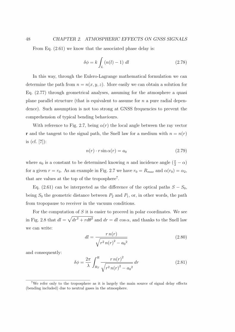
48 CHAPTER 2. ATMOSPHERIC EFFECTS ON GNSS SIGNALS
From Eq. (2.61) we know that the associated phase delay is:
δφ = k
∫L
(n(l)− 1) dl (2.78)
In this way, through the Eulero-Lagrange mathematical formulation we can
determine the path from n = n(x, y, z). More easily we can obtain a solution for
Eq. (2.77) through geometrical analyses, assuming for the atmosphere a quasi
plane parallel structure (that is equivalent to assume for n a pure radial depen-
dence). Such assumption is not too strong at GNSS frequencies to prevent the
comprehension of typical bending behaviours.
With reference to Fig. 2.7, being α(r) the local angle between the ray vector
r and the tangent to the signal path, the Snell law for a medium with n = n(r)
is (cf. [7]):
n(r) · r sinα(r) = a0 (2.79)
where a0 is a constant to be determined knowing n and incidence angle (π2− α)
for a given r = r0. As an example in Fig. 2.7 we have r0 = Rmax and α(r0) = α2,
that are values at the top of the troposphere7.
Eq. (2.61) can be interpreted as the difference of the optical paths S − S0,
being S0 the geometric distance between P2 and P1, or, in other words, the path
from tropopause to receiver in the vacuum conditions.
For the computation of S it is easier to proceed in polar coordinates. We see
in Fig. 2.8 that dl =√dr2 + rdθ2 and dr = dl cosα, and thanks to the Snell law
we can write:
dl =r n(r)√
r2 n(r)2 − a02
(2.80)
and consequently:
δφ =2π
λ
∫ R
RT
r n(r)2√r2 n(r)2 − a0
2
dr (2.81)
7We refer only to the troposphere as it is largely the main source of signal delay effects(bending included) due to neutral gases in the atmosphere.
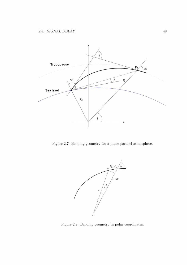
2.3. SIGNAL DELAY 49
Figure 2.7: Bending geometry for a plane parallel atmosphere.
Figure 2.8: Bending geometry in polar coordinates.
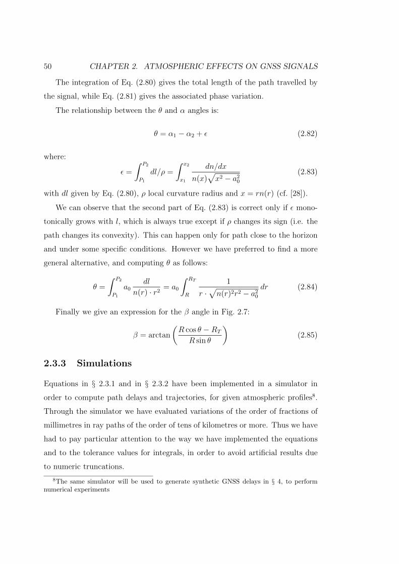
50 CHAPTER 2. ATMOSPHERIC EFFECTS ON GNSS SIGNALS
The integration of Eq. (2.80) gives the total length of the path travelled by
the signal, while Eq. (2.81) gives the associated phase variation.
The relationship between the θ and α angles is:
θ = α1 − α2 + ε (2.82)
where:
ε =
∫ P2
P1
dl/ρ =
∫ x2
x1
dn/dx
n(x)√x2 − a2
0
(2.83)
with dl given by Eq. (2.80), ρ local curvature radius and x = rn(r) (cf. [28]).
We can observe that the second part of Eq. (2.83) is correct only if ε mono-
tonically grows with l, which is always true except if ρ changes its sign (i.e. the
path changes its convexity). This can happen only for path close to the horizon
and under some specific conditions. However we have preferred to find a more
general alternative, and computing θ as follows:
θ =
∫ P2
P1
a0dl
n(r) · r2= a0
∫ RT
R
1
r ·√n(r)2r2 − a2
0
dr (2.84)
Finally we give an expression for the β angle in Fig. 2.7:
β = arctan
(R cos θ −RT
R sin θ
)(2.85)
2.3.3 Simulations
Equations in § 2.3.1 and in § 2.3.2 have been implemented in a simulator in
order to compute path delays and trajectories, for given atmospheric profiles8.
Through the simulator we have evaluated variations of the order of fractions of
millimetres in ray paths of the order of tens of kilometres or more. Thus we have
had to pay particular attention to the way we have implemented the equations
and to the tolerance values for integrals, in order to avoid artificial results due
to numeric truncations.
8The same simulator will be used to generate synthetic GNSS delays in § 4, to performnumerical experiments
2.3. SIGNAL DELAY 51
Here we present only simulations performed with standard atmospheric values
in order to fix some typical behaviours of the GNSS signal useful for the following
of the present work. Namely we have adopted:
• for the ionosphere, diurnal and nocturnal standard profiles from [5] that is
a sort of ionospheric equivalent of the standard atmosphere;
• for the wet neutral atmosphere, the standard atmosphere as described in
§ 1.2.2 and specifically through equations (1.14) and (1.15);
• for the wet atmosphere, an “extremely wet” standard tropospheric profile,
i.e. a standard profile that have been saturated in the troposphere.
Fig. 2.9 in the top panel shows a typical range of zenith delay values, where
the extremes are given by a lowest delay profile, due to a ray path crossing first
a ionosphere with a minimum (i.e. nocturnal) TEC and then a completely dry
atmosphere, and a highest delay, due to a ray path crossing first a ionosphere
with a maximum (i.e. diurnal) TEC and then a standard profile but saturated
in the troposphere. We can see how the main and more variable contribution
comes from the ionosphere, leading to zenith delays from 5 to over 30m. This is
the reason why an accurate retrieval of such term, through a multi-frequencies
signal processing (as introduced in § 2.3.1and that will be completed in § 3.4.2),
is mandatory for precise positioning as well as for tropospheric sounding. The
tropospheric delays are “only” around 2.3÷ 2.5m and from the bottom panel of
Fig. 2.10 we can see how water vapour can contribute for about a 10% of such
delays at most. From this we understand how, for tropospheric water vapour
retrieval, it is necessary to process tropospheric delays with an accuracy of the
order or better than the cm, i.e. it is necessary to set up a GNSS pre-processing
chain according to such constrain.
Non zenith ray paths lead to greater delays according to the greater thickness
of the atmospheric shell to be crossed. Such delay increments go as 1/ sinαel,
with αel elevation angle (in Fig. 2.7) the complementary of angle α1), apart from
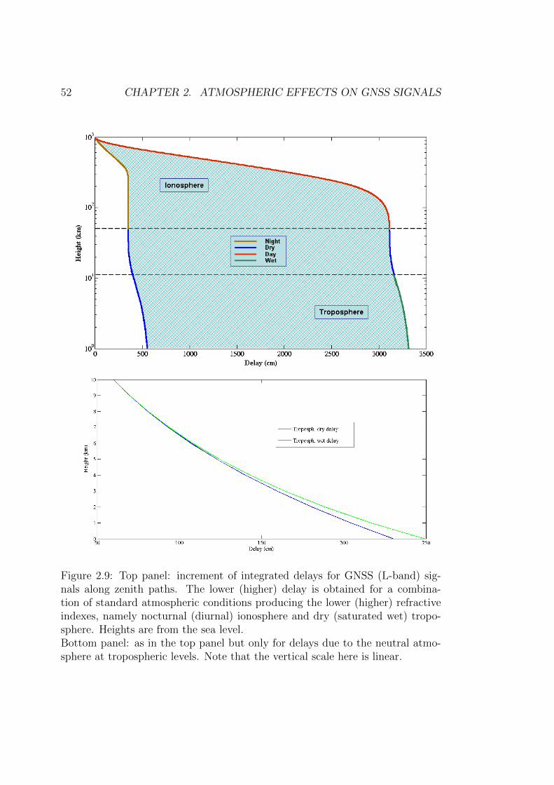
52 CHAPTER 2. ATMOSPHERIC EFFECTS ON GNSS SIGNALS
Figure 2.9: Top panel: increment of integrated delays for GNSS (L-band) sig-nals along zenith paths. The lower (higher) delay is obtained for a combina-tion of standard atmospheric conditions producing the lower (higher) refractiveindexes, namely nocturnal (diurnal) ionosphere and dry (saturated wet) tropo-sphere. Heights are from the sea level.Bottom panel: as in the top panel but only for delays due to the neutral atmo-sphere at tropospheric levels. Note that the vertical scale here is linear.
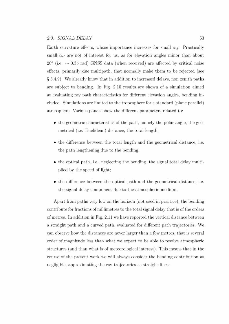
2.3. SIGNAL DELAY 53
Earth curvature effects, whose importance increases for small αel. Practically
small αel are not of interest for us, as for elevation angles minor than about
20o (i.e. ∼ 0.35 rad) GNSS data (when received) are affected by critical noise
effects, primarily due multipath, that normally make them to be rejected (see
§ 3.4.9). We already know that in addition to increased delays, non zenith paths
are subject to bending. In Fig. 2.10 results are shown of a simulation aimed
at evaluating ray path characteristics for different elevation angles, bending in-
cluded. Simulations are limited to the troposphere for a standard (plane parallel)
atmosphere. Various panels show the different parameters related to:
• the geometric characteristics of the path, namely the polar angle, the geo-
metrical (i.e. Euclidean) distance, the total length;
• the difference between the total length and the geometrical distance, i.e.
the path lengthening due to the bending;
• the optical path, i.e., neglecting the bending, the signal total delay multi-
plied by the speed of light;
• the difference between the optical path and the geometrical distance, i.e.
the signal delay component due to the atmospheric medium.
Apart from paths very low on the horizon (not used in practice), the bending
contribute for fractions of millimetres to the total signal delay that is of the orders
of metres. In addition in Fig. 2.11 we have reported the vertical distance between
a straight path and a curved path, evaluated for different path trajectories. We
can observe how the distances are never larger than a few metres, that is several
order of magnitude less than what we expect to be able to resolve atmospheric
structures (and than what is of meteorological interest). This means that in the
course of the present work we will always consider the bending contribution as
negligible, approximating the ray trajectories as straight lines.
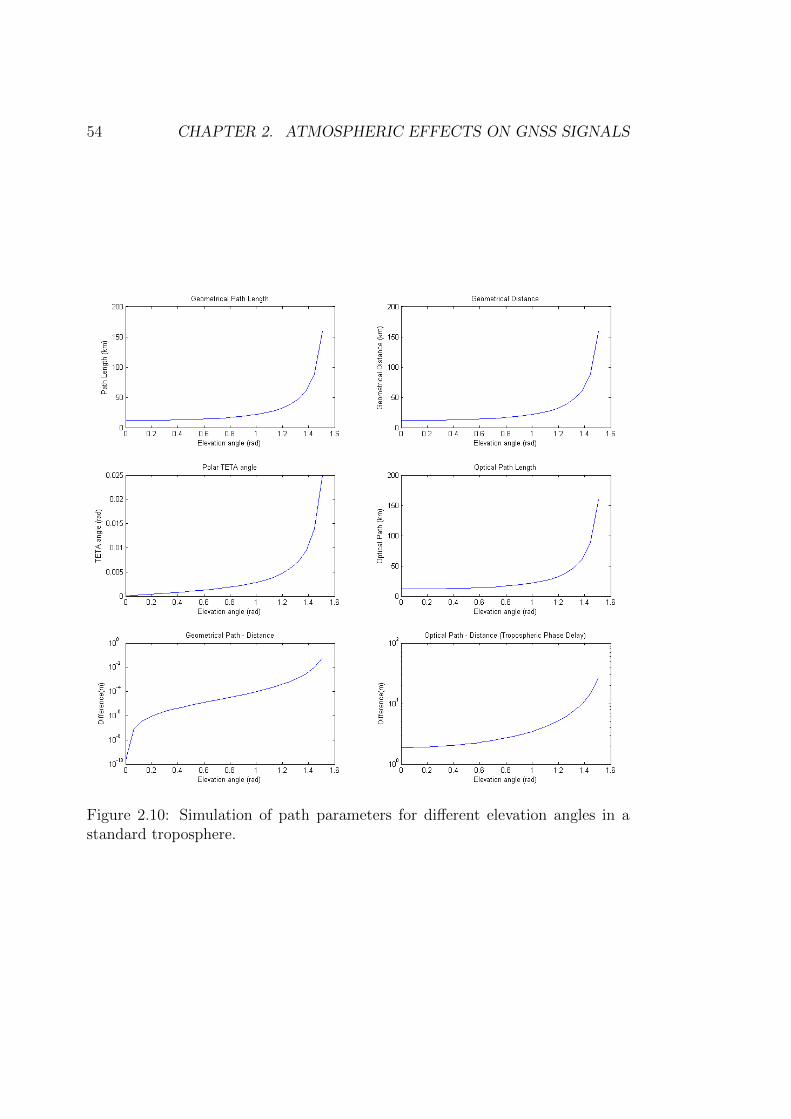
54 CHAPTER 2. ATMOSPHERIC EFFECTS ON GNSS SIGNALS
Figure 2.10: Simulation of path parameters for different elevation angles in astandard troposphere.
2.3. SIGNAL DELAY 55
Figure 2.11: Different ray trajectories (top panel) and corresponding verticaldistances between straight and curved paths due to the bending (bottom panel)in a standard troposphere.
56 CHAPTER 2. ATMOSPHERIC EFFECTS ON GNSS SIGNALS
Chapter 3
The GPS satellite navigationsystem
3.1 The basis of satellite navigation
Satellite navigation represents the last evolution in navigation, since on early
1960’s an initiative of U.S. Navy started experiments to create a system for
precise positioning. The system was called Navy Navigation Satellite System
(NNSS) or, more commonly, TRANSIT, and was developed by Johns Hopkins
Applied Physics Laboratory (APL). The first proof of concept was based on
data coming from the first artificial satellite Sputnik I (Russian satellite) and
it demonstrated the possibility to track satellite orbits using a Doppler signal
coming from a satellite, detected from points of known position on the Earth
surface. The inversion of the problem led to the first satellite radio navigation
system able to determine the position of an user by knowing the Doppler shift
of detected satellite signal and the satellite orbital parameters. The TRAN-
SIT navigation system was developed for military purposes, mainly for subma-
rine navigation. The experience of TRANSIT gave origin to the TIMATION
(TIMe/navigATION), program of Naval Research Laboratory’s (NRL’s) Naval
Center for Space Technology (NCST), which designed satellites equipped with ac-
curate oscillators (quartz oscillator in the start project phase and atomic clocks in
the final project phase) controlled and systematically re-synchronised by ground
master stations. The program started in 1967 and proved that a system based on
57
58 CHAPTER 3. THE GPS SATELLITE NAVIGATION SYSTEM
a passive ranging technique, combined with highly accurate clocks, could lead to
an unprecedented navigation system with three-dimensional coverage (longitude,
latitude, and altitude) all over the world. The results of the TIMATION pro-
gram gave the basis for the development of the first satellite based passive radio
navigation system, the NAVSTAR (Navigation System with Time and Ranging)
or Global Positioning System (GPS). GPS was the first born of a small number of
analogous systems from different countries, all belonging to the family of Global
Navigation Satellite Systems (GNSS) whose working principle is essentially the
same: the possibility to measure the distance of a receiver from satellites and
consequently to analytically solve a system of three equations with the receiver
coordinates as unknowns, provided we have (at least) three non aligned satel-
lites in view, that transmit a signal with the “exact” time of transmission and
corresponding satellite position, and that are all synchronised with the receiver
clock, that gives the exact time of signal arrival1. However for cost saving and
practical advantages, GPS receivers are not equipped with precise atomic clocks,
so they cannot be considered synchronised with the satellites: as a consequence,
the receiver time becomes an additional unknown and at least four satellites are
needed to analytically solve a system of four equations with four unknowns.
The GPS design started in 1973 and the system became fully operational
in 1993. The main services provided by GPS are user position, speed vector
determination and the time synchronisation at a global scale. The GPS system
has been designed and developed from U.S. military departments for military and
civilian users, but the performance of the system could be degraded for reason
of security, using the so called “Selective Availability” (SA). Since May 1st 2000
the SA has been turned off, and the full precision of GPS system is available for
all GPS users.
The architecture of the system consists of a space segment, a control segment
and a users segment.
1It is apparent that such a problem admits two solutions, but only one of interest becauseon the Earth surface, the other being in a point of the exosphere, which results symmetric tothe one of interest, with respect to the plane individuated by the three satellites in view.
3.2. GPS CONSTELLATION 59
The space segment is the constellation of satellites; that send a signal with
a unique code for each satellite, giving information for time synchronisation and
space vehicle position determination.
The Operational Control Segment (OCS) performs the tracking of space ve-
hicles, computing, monitoring and adjusting their positions; the monitoring of
space vehicle clock offset and drift to maintain synchronisation within the satel-
lite clocks; the updating of the navigation signal sent by satellites. The control
segment is composed by the Master Control Station (MCS) and five Monitor
Stations (MS), some of them equipped with Ground Antennas (GA).
The User Segment consists of the final users of the GPS system. The hardware
of user receivers detects the GPS satellites signals and gives the position by means
of the installed software.
The GPS system is designed to contemporarily provide two different services:
Standard Position Service (SPS) and Precise Positioning Service (PPS). At this
purpose the system is equipped with two different type of signals sent by satel-
lites, called respectively coarse acquisition (C/A) code and precision (P) code.
The system is designed to ensure the correct positioning in every place on the
Earth: this is guaranteed by the possibility to receive simultaneously data from
more than four satellite (up to ten in some cases), always and everywhere2. This
redundancy is essential when the computation is not limited to the four unknowns
which constitute the space-time position, but involves other uncertainties, e.g.
biases and offsets given by noise sources.
3.2 GPS constellation
3.2.1 Space segment structure
The Space Segment consists on the GPS satellite constellation. At the moment
there are 31 operational satellites. For redundancy reasons they are more than
the minimum number ensuring the proper system coverage, which is 24. The
2Of course this is true except when signal reception is obstructed by local shields.
60 CHAPTER 3. THE GPS SATELLITE NAVIGATION SYSTEM
satellites are arranged on 6 orbital planes, each of them containing at least 4 slots
where satellites can be equidistantly set. The orbital planes have an inclination
of 55 with respect to the equatorial plane and are rotated in the equatorial plane
by 60 against each other. This geometry ensures total global coverage so that
at least four satellites are simultaneously visible anytime and anywhere, allowing
to take advantage of the positioning service. The GPS orbits are Medium Earth
Orbit (MEO) near circular with a radius of about 26560 km, resulting in an eight
of 20200 km above the Earth surface. The revolution time is half a sidereal day,
precisely corresponding to 11 hours and 58 minutes. The speed of GPS satellites
is about 3.9 km/s.
3.2.2 Building up of the GPS constellation
The constellation of first generation (block I) GPS satellites, consisted of 10
satellites with one caesium and two rubidium atomic clocks, that were launched
from 1978 to 1985. These satellites were experimental and are unused since
years. Block I satellites constituted the GPS Demonstration system and reflected
various stages of system development.
The second generation (block II) of 9 satellites constellation was launched
from 1989 to 1990, with the main objective of testing 14 days of operations
without contact with the Control Segment (CS). It was followed by un upgraded
generation of satellites (block IIA) consisting of 19 satellite, launched between
1990 and 1997. These satellites were designed to provide 180 days of operation
without contact from the control segment. During this autonomy period, accu-
racy degradation was verified in the navigation message. The block II and IIA
satellites are equipped with two rubidium and two caesium atomic clocks. They
have the Selective Availability (SA) and Anti-Spoof (A-S) capabilities.
When the GPS system became operational in 1993 the constellation of 24
satellites was composed by blocks I, II and IIA.
Later, 12 satellites of block IIR where successfully launched between 1997 and
2004. They were called “Replenishment” satellites. An important innovation was
3.2. GPS CONSTELLATION 61
the capability to autonomously navigate themselves (AUTONAV), by creating
the 50 Hz navigation. This includes the ability to determine thier own position
by performing inter-satellite ranging with other IIR space vehicles.
Following 8 satellites of block IIR-M, (Modernisation) were launched between
September 2005 and August 2009. The IIR-M capabilities include developmental
military-use-only M-code on the L1 and L2 signals and a civil code on the L2
signal, known as the L2C signal.
Both block IIR and block IIR-M are equipped with three rubidium atomic
clocks. Their extreme precision of about 1 second in 1 million years is absolutely
necessary for the functioning of the system, as we shall see later.
The last generation of on orbit GPS satellites is the block IIF. The first
satellite of this block was launched in May 2010. These satellite are functionally
equivalent to the IIR/IIR-M satellites and pave the way towards operational M-
code and L2C signal. The improvement introduced by this satellite generation
involves converting the GPS caesium clocks from analog to digital. Block IIF
also adds a new separate signal for civilian use, designated L5 at the frequency
of 1176.45 MHz. These two codes mark the transition to the GPS III era.
3.2.2.1 the future GPS III
GPS III block will give new navigation warfare (NAVWAR) capabilities to shut
off GPS service for security reasons, but only on limited geographical locations.
The new system will offer significant improvements in navigation capabilities by
new navigation signals:
• The M-code, signal transmitted in the same L1 and L2 frequencies already
in use by the previous military code, the P(Y) code. It is designed to be
autonomous, meaning that users can calculate their positions using only the
M-code signal. It will be broadcast from a high-gain directional antenna,
in addition to a wide angle (full Earth) antenna.
• The civilian L2 (L2C) signal, providing improved accuracy of navigation,
62 CHAPTER 3. THE GPS SATELLITE NAVIGATION SYSTEM
and acting as a redundant signal in case of localised interference (in addition
to the opportunity of correcting for ionospheric effects)
• The Safety of Life (L5) signal, a civilian-use signal, broadcast on the L5
frequency (1176.45 MHz), implemented since the first GPS IIF launch.
• The further L1 civilian-use (L1C) signal, to be broadcast on the same
L1 frequency (1575.42 MHz) that currently contains the C/A signal used
by all current GPS users. The L1C will be available with first Block III
launch, currently scheduled for 2013. The L1 signal will be interoperable
with Galileo satellite navigation system.
• A further frequency (L4) will be available at 1379.913 MHz and will be
under study for improved ionospheric correction.
All these new signals will be transmitted with increased power and wider band-
width and will ensure improvements on the services which they drive. The full
operational constellation will consist of 32 satellites.
The GPS III system will provide also information about worldwide localisa-
tion of signals of nuclear detonations, through the Nuclear detonation Detection
System payload (NDS).
3.2.3 Satellite instruments
All satellites are equipped with dual solar arrays supplying over 400 W . A S-
Band communication link (2227.5 MHz) is used for control and telemetry. A
UHF channel provides cross-links among spacecrafts. A propulsion system is
used for orbital correction.
The core of the payload includes two L-Band navigation signals, L1
at 1575.42 MHz and L2 at 1227.60 MHz, locally generated by means ofpre-
cise atomic oscillators. The antenna for the navigation signals sends Right-Hand
Circularly Polarised (RHCP) waves.
3.2. GPS CONSTELLATION 63
3.2.3.1 Transmitter and receiver clocks
Precise measurements of time are crucial in GNSS positioning. Satellite clock
reference and clock offset parameters are also included in the navigation message,
because normal receiver clocks are not synchronised with satellite ones.
The core of the satellite payload is the atomic oscillator. Currently all satel-
lites are provided by two Rubidium and two Caesium atomic clocks. One of
these atomic standards is designated as primary and serves as timing reference
on board of the space vehicle for navigation signal generation and transmission.
These extremely accurate GPS atomic clocks must keep time to within a few
nanoseconds a day and they are synchronised. Despite the extreme precision, if
the satellite clock drifts and offsets are not taken into account, the resulting error
in the positioning can become quite large. Furthermore the correction cannot
be applied to the satellite clock, therefore drifts and clocks add up. The Mas-
ter Control Station (in Colorado Springs), collects all satellite data received by
all the Control Segment stations and systematically they update parameters for
orbits and clock synchronisation. Parameters for satellite clock correction are
provided in the navigation message by means of coefficients of a second order
polynomial interpolation:
te = a0 + a1(t− tr) + a2(t− tr)2 (3.1)
where: a0, a1, a2 are the polynomial coefficients; te is the estimated (corrected)
time; tr is the reference time for the parameters computation; t is the clock
uncorrected time.
These parameters are uploaded to the satellites for realtime broadcast, pro-
viding the real time positioning and timing services.
The stability and accuracy of a clock is often presented in terms of Allan
variance:
σ2A =
⟨[φ(t+ 2τ)− 2φ(t+ τ) + φ(t)]2
2τω0
⟩(3.2)
where: σ2A(τ) is the Allan variance; τ is the averaging time; φ(t) is the clock
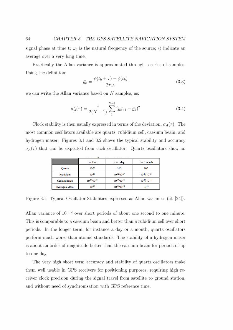
64 CHAPTER 3. THE GPS SATELLITE NAVIGATION SYSTEM
signal phase at time t; ω0 is the natural frequency of the source; 〈〉 indicate an
average over a very long time.
Practically the Allan variance is approximated through a series of samples.
Using the definition:
yk =φ(tk + τ)− φ(tk)
2τω0
(3.3)
we can write the Allan variance based on N samples, as:
σ2A(τ) =
1
2(N − 1)
N−1∑1
( ¯yk+1 − yk)2 (3.4)
Clock stability is then usually expressed in terms of the deviation, σA(τ). The
most common oscillators available are quartz, rubidium cell, caesium beam, and
hydrogen maser. Figures 3.1 and 3.2 shows the typical stability and accuracy
σA(τ) that can be expected from each oscillator. Quartz oscillators show an
Figure 3.1: Typical Oscillator Stabilities expressed as Allan variance. (cf. [24]).
Allan variance of 10−12 over short periods of about one second to one minute.
This is comparable to a caesium beam and better than a rubidium cell over short
periods. In the longer term, for instance a day or a month, quartz oscillators
perform much worse than atomic standards. The stability of a hydrogen maser
is about an order of magnitude better than the caesium beam for periods of up
to one day.
The very high short term accuracy and stability of quartz oscillators make
them well usable in GPS receivers for positioning purposes, requiring high re-
ceiver clock precision during the signal travel from satellite to ground station,
and without need of synchronisation with GPS reference time.
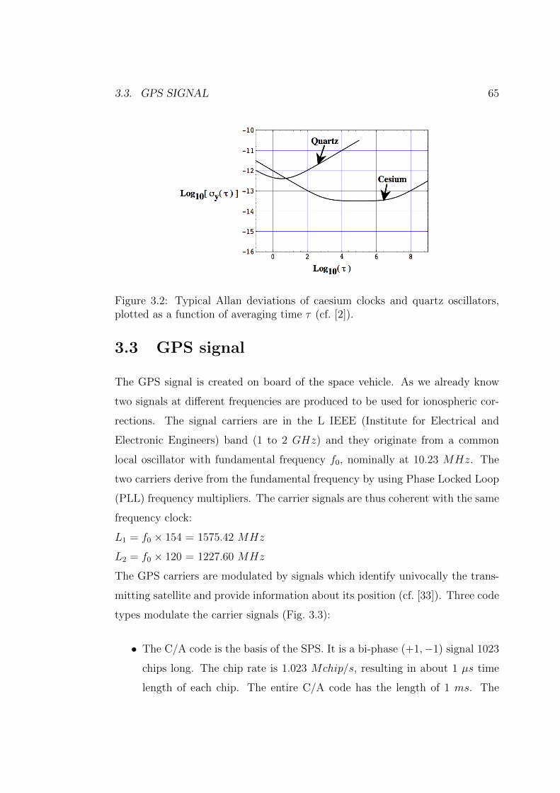
3.3. GPS SIGNAL 65
Figure 3.2: Typical Allan deviations of caesium clocks and quartz oscillators,plotted as a function of averaging time τ (cf. [2]).
3.3 GPS signal
The GPS signal is created on board of the space vehicle. As we already know
two signals at different frequencies are produced to be used for ionospheric cor-
rections. The signal carriers are in the L IEEE (Institute for Electrical and
Electronic Engineers) band (1 to 2 GHz) and they originate from a common
local oscillator with fundamental frequency f0, nominally at 10.23 MHz. The
two carriers derive from the fundamental frequency by using Phase Locked Loop
(PLL) frequency multipliers. The carrier signals are thus coherent with the same
frequency clock:
L1 = f0 × 154 = 1575.42 MHz
L2 = f0 × 120 = 1227.60 MHz
The GPS carriers are modulated by signals which identify univocally the trans-
mitting satellite and provide information about its position (cf. [33]). Three code
types modulate the carrier signals (Fig. 3.3):
• The C/A code is the basis of the SPS. It is a bi-phase (+1,−1) signal 1023
chips long. The chip rate is 1.023 Mchip/s, resulting in about 1 µs time
length of each chip. The entire C/A code has the length of 1 ms. The
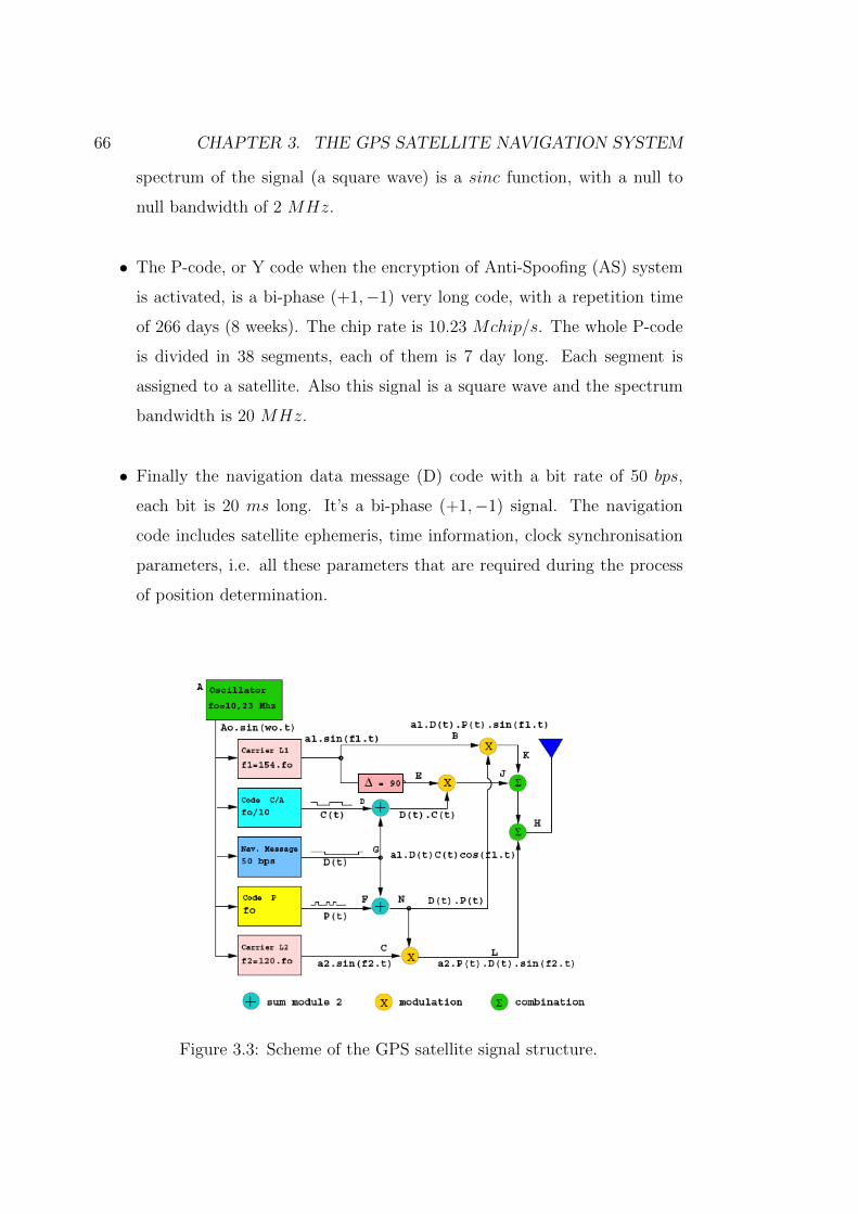
66 CHAPTER 3. THE GPS SATELLITE NAVIGATION SYSTEM
spectrum of the signal (a square wave) is a sinc function, with a null to
null bandwidth of 2 MHz.
• The P-code, or Y code when the encryption of Anti-Spoofing (AS) system
is activated, is a bi-phase (+1,−1) very long code, with a repetition time
of 266 days (8 weeks). The chip rate is 10.23 Mchip/s. The whole P-code
is divided in 38 segments, each of them is 7 day long. Each segment is
assigned to a satellite. Also this signal is a square wave and the spectrum
bandwidth is 20 MHz.
• Finally the navigation data message (D) code with a bit rate of 50 bps,
each bit is 20 ms long. It’s a bi-phase (+1,−1) signal. The navigation
code includes satellite ephemeris, time information, clock synchronisation
parameters, i.e. all these parameters that are required during the process
of position determination.
Figure 3.3: Scheme of the GPS satellite signal structure.
3.3. GPS SIGNAL 67
Signals SL1 and SL2 at two frequencies, can be expressed as:
SL1 = APPk(t)Dk(t)cos(2πf1t+ φ) + AC C/Ak(t)Dk(t)sin(2πf1t+ φ)
SL2 = APPk(t)Dk(t)cos(2πf2t+ φ) (3.5)
where:
AP is the amplitude of the P-code
Pk(t) is the precision code (± 1) for the kth satellite
Dk(t) is the navigation code (± 1) for the kth satellite
AC is the amplitude of the C/A code
C/Ak(t) is the coarse acquisition code (± 1) for the kth satellite
φ is the initial phase of the signal
The GPS signal is a phase-modulated signal with phase φ = (0, π); this type
of phase modulation is referred to as Binary Phase Shift Keying (BPSK).
Coarse Acquisition (C/A) and Precision (P) codes are in quadrature to allow
a best detection of the signal.
The code signals can reach a minimum power level of −130 dBm and the
spectrum is spread; so they cannot be detected from a spectrum analyser. The
Spread Spectrum Modulation (SSM) is used to transmit the signal and the use of
the Code Division Multiple Access (CDMA) allows to use the same band portion
and the same centre frequency for all the signals transmission.
The codes (C/A and P) relative to different satellites are orthogonal: their
cross correlation and their autocorrelation, computed for a non-zero shift delay,
are very low. The autocorrelation function has a strong peak when the shift delay
is zero, so that the receiver can accurately reconstruct and decode the signal.
Often these codes are referred as Pseudo Random Noise (PRN), because the
white noise has an autocorrelation function essentially with the same properties.
At the receiver level, codes of each signals must be generated and used to
correlate with the received satellite signals, for decoding the information content.
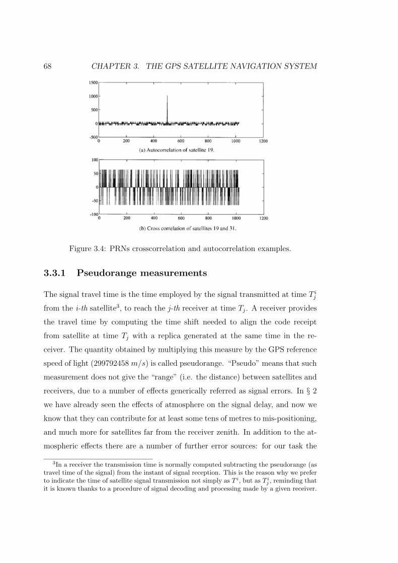
68 CHAPTER 3. THE GPS SATELLITE NAVIGATION SYSTEM
Figure 3.4: PRNs crosscorrelation and autocorrelation examples.
3.3.1 Pseudorange measurements
The signal travel time is the time employed by the signal transmitted at time T ij
from the i-th satellite3, to reach the j-th receiver at time Tj. A receiver provides
the travel time by computing the time shift needed to align the code receipt
from satellite at time Tj with a replica generated at the same time in the re-
ceiver. The quantity obtained by multiplying this measure by the GPS reference
speed of light (299792458 m/s) is called pseudorange. “Pseudo” means that such
measurement does not give the “range” (i.e. the distance) between satellites and
receivers, due to a number of effects generically referred as signal errors. In § 2
we have already seen the effects of atmosphere on the signal delay, and now we
know that they can contribute for at least some tens of metres to mis-positioning,
and much more for satellites far from the receiver zenith. In addition to the at-
mospheric effects there are a number of further error sources: for our task the
3In a receiver the transmission time is normally computed subtracting the pseudorange (astravel time of the signal) from the instant of signal reception. This is the reason why we preferto indicate the time of satellite signal transmission not simply as T i, but as T ij , reminding thatit is known thanks to a procedure of signal decoding and processing made by a given receiver.
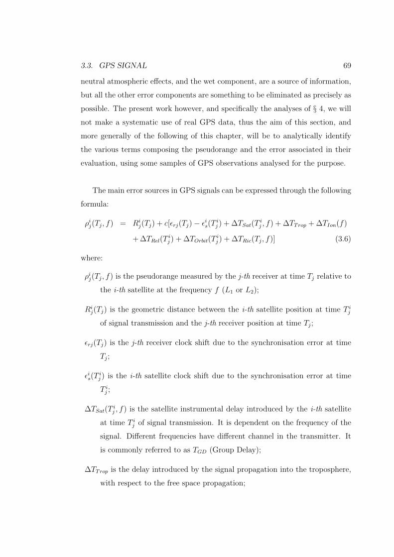
3.3. GPS SIGNAL 69
neutral atmospheric effects, and the wet component, are a source of information,
but all the other error components are something to be eliminated as precisely as
possible. The present work however, and specifically the analyses of § 4, we will
not make a systematic use of real GPS data, thus the aim of this section, and
more generally of the following of this chapter, will be to analytically identify
the various terms composing the pseudorange and the error associated in their
evaluation, using some samples of GPS observations analysed for the purpose.
The main error sources in GPS signals can be expressed through the following
formula:
ρij(Tj, f) = Rij(Tj) + c[εrj(Tj)− εis(T ij ) + ∆TSat(T
ij , f) + ∆TTrop + ∆TIon(f)
+ ∆TRel(Tij ) + ∆TOrbit(T
ij ) + ∆TRic(Tj, f)] (3.6)
where:
ρij(Tj, f) is the pseudorange measured by the j-th receiver at time Tj relative to
the i-th satellite at the frequency f (L1 or L2);
Rij(Tj) is the geometric distance between the i-th satellite position at time T ij
of signal transmission and the j-th receiver position at time Tj;
εrj(Tj) is the j-th receiver clock shift due to the synchronisation error at time
Tj;
εis(Tij ) is the i-th satellite clock shift due to the synchronisation error at time
T ij ;
∆TSat(Tij , f) is the satellite instrumental delay introduced by the i-th satellite
at time T ij of signal transmission. It is dependent on the frequency of the
signal. Different frequencies have different channel in the transmitter. It
is commonly referred to as TGD (Group Delay);
∆TTrop is the delay introduced by the signal propagation into the troposphere,
with respect to the free space propagation;
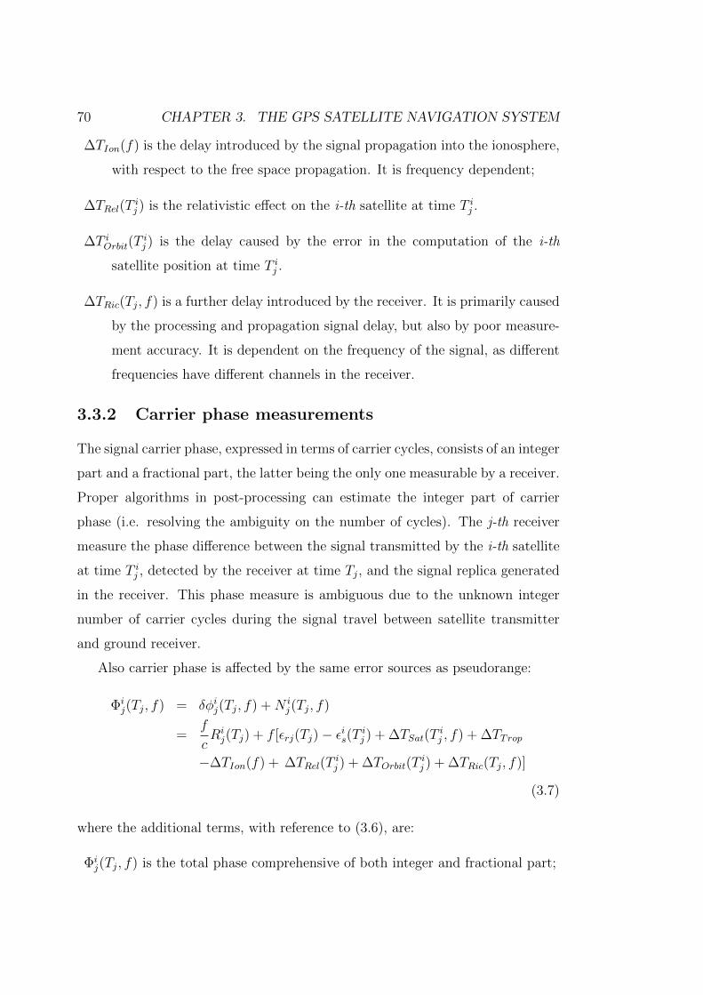
70 CHAPTER 3. THE GPS SATELLITE NAVIGATION SYSTEM
∆TIon(f) is the delay introduced by the signal propagation into the ionosphere,
with respect to the free space propagation. It is frequency dependent;
∆TRel(Tij ) is the relativistic effect on the i-th satellite at time T ij .
∆T iOrbit(Tij ) is the delay caused by the error in the computation of the i-th
satellite position at time T ij .
∆TRic(Tj, f) is a further delay introduced by the receiver. It is primarily caused
by the processing and propagation signal delay, but also by poor measure-
ment accuracy. It is dependent on the frequency of the signal, as different
frequencies have different channels in the receiver.
3.3.2 Carrier phase measurements
The signal carrier phase, expressed in terms of carrier cycles, consists of an integer
part and a fractional part, the latter being the only one measurable by a receiver.
Proper algorithms in post-processing can estimate the integer part of carrier
phase (i.e. resolving the ambiguity on the number of cycles). The j-th receiver
measure the phase difference between the signal transmitted by the i-th satellite
at time T ij , detected by the receiver at time Tj, and the signal replica generated
in the receiver. This phase measure is ambiguous due to the unknown integer
number of carrier cycles during the signal travel between satellite transmitter
and ground receiver.
Also carrier phase is affected by the same error sources as pseudorange:
Φij(Tj, f) = δφij(Tj, f) +N i
j(Tj, f)
=f
cRij(Tj) + f [εrj(Tj)− εis(T ij ) + ∆TSat(T
ij , f) + ∆TTrop
−∆TIon(f) + ∆TRel(Tij ) + ∆TOrbit(T
ij ) + ∆TRic(Tj, f)]
(3.7)
where the additional terms, with reference to (3.6), are:
Φij(Tj, f) is the total phase comprehensive of both integer and fractional part;
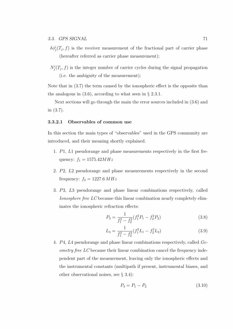
3.3. GPS SIGNAL 71
δφij(Tj, f) is the receiver measurement of the fractional part of carrier phase
(hereafter referred as carrier phase measurement);
N ij(Tj, f) is the integer number of carrier cycles during the signal propagation
(i.e. the ambiguity of the measurement);
Note that in (3.7) the term caused by the ionospheric effect is the opposite than
the analogous in (3.6), according to what seen in § 2.3.1.
Next sections will go through the main the error sources included in (3.6) and
in (3.7).
3.3.2.1 Observables of common use
In this section the main types of “observables” used in the GPS community are
introduced, and their meaning shortly explained.
1. P1, L1 pseudorange and phase measurements respectively in the first fre-
quency: f1 = 1575.42MHz
2. P2, L2 pseudorange and phase measurements respectively in the second
frequency: f2 = 1227.6MHz
3. P3, L3 pseudorange and phase linear combinations respectively, called
Ionosphere free LC because this linear combination nearly completely elim-
inates the ionospheric refraction effects:
P3 =1
f 21 − f 2
2
(f 21P1 − f 2
2P2) (3.8)
L3 =1
f 21 − f 2
2
(f 21L1 − f 2
2L2) (3.9)
4. P4, L4 pseudorange and phase linear combinations respectively, called Ge-
ometry free LC because their linear combination cancel the frequency inde-
pendent part of the measurement, leaving only the ionospheric effects and
the instrumental constants (multipath if present, instrumental biases, and
other observational noises, see § 3.4):
P4 = P1 − P2 (3.10)
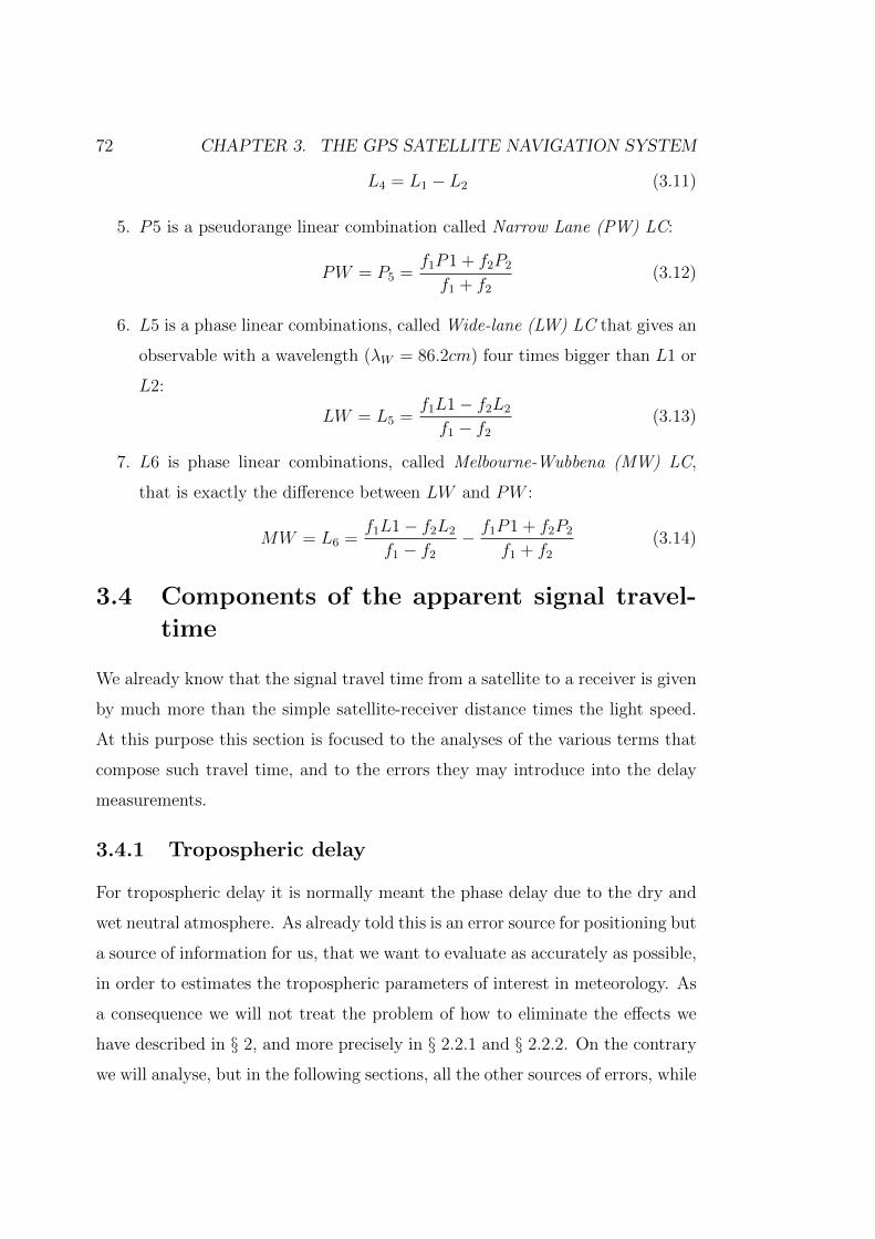
72 CHAPTER 3. THE GPS SATELLITE NAVIGATION SYSTEM
L4 = L1 − L2 (3.11)
5. P5 is a pseudorange linear combination called Narrow Lane (PW) LC:
PW = P5 =f1P1 + f2P2
f1 + f2
(3.12)
6. L5 is a phase linear combinations, called Wide-lane (LW) LC that gives an
observable with a wavelength (λW = 86.2cm) four times bigger than L1 or
L2:
LW = L5 =f1L1− f2L2
f1 − f2
(3.13)
7. L6 is phase linear combinations, called Melbourne-Wubbena (MW) LC,
that is exactly the difference between LW and PW :
MW = L6 =f1L1− f2L2
f1 − f2
− f1P1 + f2P2
f1 + f2
(3.14)
3.4 Components of the apparent signal travel-
time
We already know that the signal travel time from a satellite to a receiver is given
by much more than the simple satellite-receiver distance times the light speed.
At this purpose this section is focused to the analyses of the various terms that
compose such travel time, and to the errors they may introduce into the delay
measurements.
3.4.1 Tropospheric delay
For tropospheric delay it is normally meant the phase delay due to the dry and
wet neutral atmosphere. As already told this is an error source for positioning but
a source of information for us, that we want to evaluate as accurately as possible,
in order to estimates the tropospheric parameters of interest in meteorology. As
a consequence we will not treat the problem of how to eliminate the effects we
have described in § 2, and more precisely in § 2.2.1 and § 2.2.2. On the contrary
we will analyse, but in the following sections, all the other sources of errors, while
3.4. COMPONENTS OF THE APPARENT SIGNAL TRAVEL-TIME 73
the discussion on how to retrieve the searched information from the tropospheric
delay will be dealt in § 4.
3.4.2 Ionospheric delay
In § 2.2.3and § 2.3.1we have already seen the origin of a refraction index in
ionosphere that results smaller than 1, namely on average n : n− 1 ∼ 10−5. We
have also commented that this implies a phase advance and a group delay that
are equal in magnitude, apart from bending effects.
The difference ∆τ between group delays, as in Eq. (2.76), and phase advances,
as in Eq. (2.75), obtained in the two different frequencies L1 and L2, can be
written as:
∆τ = B
[1
f 2L2
− 1
f 2L1
]=
B
f 2L2
[f 2L1 − f 2
L2
f 2L1
]= ∆TIon(fL2)
[1− f 2
L2
f 2L1
]... = ∆TIon(fL1)
[f 2L1
f 2L2
− 1
](3.15)
where B = αTEC.
Considering P1 e P2 the pseudorange measurements with the precision-code,
by assuming negligible the variation with the frequency of all terms present in
Eq. (3.6):
∆T P2Ion(fL2) =
[P2 − P1]
c
f 2L1
f 2L1 − f 2
L2
∆T P1Ion(fL1) =
[P2 − P1]
c
f 2L2
f 2L1 − f 2
L2
(3.16)
Unfortunately the frequency dependent terms, introduced by the satellite and
receiver hardware, are not negligible and must be carefully modelled in order
to correctly retrieve the ionosphere effect, as we will see later. On the contrary
the precision in the approximation of Eq. (2.59) are generally very accurate,
but, under some conditions, they can result precise at the 1 % or less: for high
TEC values this means to have errors of several centimetres or more (for zenith
observations). This can be too big an error for atmospheric sounding; in any
case from Eq. (2.60) the value of such approximations can be evaluated.
74 CHAPTER 3. THE GPS SATELLITE NAVIGATION SYSTEM
Finally it is worth to note that it is not possible to process only carrier phase
measurements in two different frequencies for computing the ionospheric delay,
because of the ambiguities. Some ancillary information must be used for solving
these ambiguities, such as pseudorange measurements.
3.4.3 Relativistic effects
In order to determine the orbits of satellites, the GPS system uses an inertial
Cartesian coordinate system, the Earth Centred Inertial (ECI) reference system
in which the origin is at the centre of mass of the Earth, the x-y plane is coinci-
dent with the Earth’s equatorial plane and the x and y axes are oriented along
determined positions over the celestial sphere; the z axis is normal to the x-y
plane in the north direction.
Non inertial motions (i.e. satellite orbits and Earth rotation) and the Earth
gravitational field make relativistic effects non negligible with respect to signal
accuracy constrains.
A first effect regards the change in the signal frequency. The nominal fre-
quency of 10, 23MHz at a ground receiver is however guaranteed by a pre-launch
proper shift in the atomic oscillator frequency, that accounts for the in-orbit av-
erage relativistic effect, as follows:
−f0 − f ′
f ′=
1
2
(vc
)2
+∆U
c2(3.17)
Where f ′ is the working frequency, f0 is the nominal frequency (10.23MHz), v
is the mean satellite speed, c is the light speed, and ∆U is the mean gravitational
potential difference between satellite and receiver. It is found f ′ = 10.23× 10⁶−
4.567× 10⁻³MHz.
Eq. (3.17) relationship considers a circular orbit for GPS satellites. To take
into account for the orbit eccentricity (that has consequences in the gravitational
potential differences) a correction must be applied to the pseudorange and carrier
phase relationships (3.6) and (3.7):
∆TRel =2√µa
c2e sinE (3.18)
3.4. COMPONENTS OF THE APPARENT SIGNAL TRAVEL-TIME 75
where µ = 3986005×108m3
s2is the product of the universal gravitational constant
and the Earth mass, a is the semimajor axis, e is the orbit eccentricity and E is
the eccentric anomaly (to be computed using the Kepler equation). a and e are
part of the broadcast ephemeris.
In any case some other relativistic effects caused by the orbit oscillations,
perturbations on the Earth gravitational field etc., persist. Furthermore the
satellite and receiver relative motions can produce a Doppler effect approximately
within ±5 KHz.
These effects can be modelled for precise estimations in order to give negligible
contribution to the overall error in positioning or, in the case of our interest, in
the tropospheric delay evaluation. Here follows some major terms.
The Holdridge model (cf. [48]) accounts for general relativity effects on the
signal delay:
δρRel =2µ
c2lnρj + ρi + ρijρj + ρi − ρij
(3.19)
where: ρj is the geocentric position of the j-th receiver, ρi is the geocentric
position of the i-th satellite, ρij is the geocentric distance between the j-th receiver
and the i-th satellite.
δρRel can reach a maximum value of about 2 cm.
The correction for the acceleration of the Earth satellite, following the model
of McCarthy (cf. [48]):
∆~a =µ
c2r3
[4µ
r− v2
]~r + 4(~r · ~v)~v
(3.20)
where ~r is the geocentric satellite position vector, ~v is the geocentric satellite
velocity vector and ~a is the geocentric satellite acceleration vector.
In addition to all the previous terms, there is a further factor due to relative
motions of satellites and receivers. A receiver can be generally in motion on the
Earth’s surface. For our purposes however only receivers with fixed position over
the Earth surface will be taken into account. Thus the only additional effect
that we have to consider is known as Sagnac effect, which is due to the Earth
rotation during the signal travel time. This effect will be treated in § 3.4.6.
76 CHAPTER 3. THE GPS SATELLITE NAVIGATION SYSTEM
3.4.4 Instrumental delays and differential code biases
There are different instrumental biases for different codes and different frequen-
cies. The available pseudorange observables are C1 (C/A code pseudorange on
the f1 frequency), P1 (P-code pseudorange on the f1 frequency), P2 (P-code
pseudorange on the f2 frequency). For each one we can identify the following
biases:
• BC1 : bias on the C1 observable
• BP1 : bias on the P1 observable
• BP2 : bias on the P2 observable
As these biases are from instruments there are two of them for each observable,
one produced by the satellite and the other from the receiver. Separately for
the satellite and for the receiver we have to consider the discrepancies between
“True” (corrected from the biases) and “Measured” (affected by biases) values:
CM1 = CT
1 +BC1
PM1 = P T
1 +BP1
PM2 = P T
2 +BP2 (3.21)
The single biases are generally not retrievable in their absolute values, because
they are generated by fluctuations in the performances of the various instruments
caused by changes of work conditions (e.g. temperature) and status (wear) and
because the instrumental biases of receiver and satellite are adds up into mea-
surements, so it is common the use of biases combinations, usuallt referred to as
Differential Code Biases (DCB):
BP1−P2 = BP1 −BP2
BP1−C1 = BP1 −BC1 (3.22)
These combination cannot directly be applied for a single observable correction,
but to a combination of observables. For example considering the availability

3.4. COMPONENTS OF THE APPARENT SIGNAL TRAVEL-TIME 77
of observables C1 and P2 from a receiver, the known approximated model of
pseudoranges (see 3.6), by neglecting the time (transmission and reception) de-
pendence, can be written :
C1ij = Rij + c[εrj − εis + ∆TTrop + ∆TIon(f1) + ∆T iRel + ∆T iOrbit +BC1]
P1ij = Rij + c[εrj − εis + ∆TTrop + ∆TIon(f1) + ∆T iRel + ∆T iOrbit +BP1]
P2ij = Rij + c[εrj − εis + ∆TTrop + ∆TIon(f1) + ∆T iRel + ∆T iOrbit +BP2]
(3.23)
where
BC1 = ∆TSat(Tij , C1)+∆TRic(Tj, C1) is the bias introduced on the C1 observable
by the instrumental delays of the satellite and the receiver;
BP1 = ∆TSat(Tij , P1)+∆TRic(Tj, P1) is the bias introduced on the P1 observable
by the instrumental delays of the satellite and the receiver;
BP2 = ∆TSat(Tij , P2)+∆TRic(Tj, P2) is the bias introduced on the P2 observable
by the instrumental delays of the satellite and the receiver.
The computation of the delay introduced by the ionosphere, as previously men-
tioned, involves the combination of the dual frequency observations:
∆TIon(f2) =[P2 − C1]
c
f 21
f 21 − f 2
2
∆TIon(f1) =[P2 − C1]
c
f 22
f 21 − f 2
2
(3.24)
Therefore, in the computation of the ionospheric delay, we have to compute
the quantity:
P2 − C1 = ∆TIon(f2)−∆TIon(f1) +BP2 −BC1
= ∆TIon(f2)−∆TIon(f1)−BP1 +BP2 +BP1 −BC1
= ∆TIon(f2)−∆TIon(f1)−BP1−P2 +BP1−C1 (3.25)
Differential Code Biases have thus to be known for the complete correction
of the ionospheric delay.
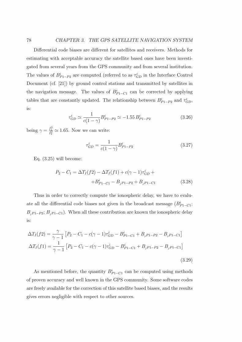
78 CHAPTER 3. THE GPS SATELLITE NAVIGATION SYSTEM
Differential code biases are different for satellites and receivers. Methods for
estimating with acceptable accuracy the satellite based ones have been investi-
gated from several years from the GPS community and from several institution.
The values of BiP1−P2 are computed (referred to as τ iGD in the Interface Control
Document (cf. [21]) by ground control stations and transmitted by satellites in
the navigation message. The values of BiP1−C1 can be corrected by applying
tables that are constantly updated. The relationship between BiP1−P2 and τ iGD,
is:
τ iGD '1
c(1− γ)BiP1−P2 ' −1.55Bi
P1−P2 (3.26)
being γ =f21f22' 1.65. Now we can write:
τ iGD =1
c(1− γ)BiP1−P2 (3.27)
Eq. (3.25) will become:
P2 − C1 = ∆TI(f2)−∆TI(f1) + c(γ − 1)τ iGD +
+BiP1−C1 −BjP1−P2 +B
jP1−C1 (3.28)
Thus in order to correctly compute the ionospheric delay, we have to evalu-
ate all the differential code biases not given in the broadcast message (BiP1−C1;
BjP1−P2; B
jP1−C1). When all these contribution are known the ionospheric delay
is:
∆TI(f2) =γ
γ − 1
[P2 − C1 − c(γ − 1)τ iGD −Bi
P1−C1 +BjP1−P2 −BjP1−C1
]∆TI(f1) =
1
γ − 1
[P2 − C1 − c(γ − 1)τ iGD −Bi
P1−C1 +BjP1−P2 −BjP1−C1
](3.29)
As mentioned before, the quantity BiP1−C1 can be computed using methods
of proven accuracy and well known in the GPS community. Some software codes
are freely available for the correction of this satellite based biases, and the results
gives errors negligible with respect to other sources.
3.4. COMPONENTS OF THE APPARENT SIGNAL TRAVEL-TIME 79
On the contrary for the computation of the receiver based DCBs there are no
standard methods or tables to refer to. In order to make an approximate estima-
tion for DCBs, we have compared measures from some GPS stations in Tuscany
with theoretical delays obtained from an established model of ionosphere. Such
model is the Klobuchar model (cf. [25]), which can estimate ionospheric effects,
and that is used as reference model by the GPS community, generally to remove
ionospheric effects from one band signals.
The Klobuchar model allows to compute the ionospheric TEC by means of
some algorithms that parameterise the sun activity. In order to correct for sea-
sonal and sun spot number changes, the algorithm uses different sets of eight
coefficients depending upon the period of the year and the average solar flux.
Better estimations are obtained during night periods, when part of the ionisa-
tion relaxes towards more stable (and known) values (see § sez:iono).
Fig. 3.5 shows in the same plot the ionospheric delay computed by using
Eq. (3.29), including correction for satellite instrumental delays, and the iono-
spheric delay as evaluated through the Klobuchar model for the same period.
The ionospheric delay computed using two frequencies is affected by receiver
DCBs. The comparison with the Klobuchar data during the minimum value
of TEC relative to minimum values of sun effects (i.e. night time close to the
sunset and for high satellite elevation angles) can be used to estimate a receiver
DCB (comprehensive of BjP1−P2 and B
jP1−C1), as a free parameter whose value
minimises the distance of the two curve minima.
In this case a delay of around −3m seems to be imputable to the receiver
DCB: it is clear that the capability of accurately estimating DCBs and their
time variability is critical for a successful retrieval of atmospheric parameters
from fixed stations.
3.4.5 Orbit parameters errors
Ephemeris data, broadcast in the satellite navigation message, give the satellite
positions as a function of time. They are predicted starting from satellite po-
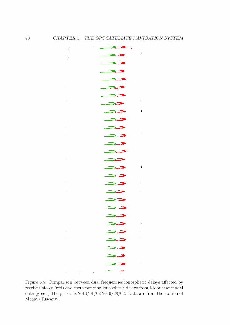
80 CHAPTER 3. THE GPS SATELLITE NAVIGATION SYSTEM
Figure 3.5: Comparison between dual frequencies ionospheric delays affected byreceiver biases (red) and corresponding ionospheric delays from Klobuchar modeldata (green).The period is 2010/01/02-2010/28/02. Data are from the station ofMassa (Tuscany).
3.4. COMPONENTS OF THE APPARENT SIGNAL TRAVEL-TIME 81
sitions regularly verified at the ground control stations. Typically, overlapping
intervals of 4 hours of GPS data are used by the operational control system to
update satellite orbital elements for a following period of 1 hour.
Ephemeris errors can be of 2 m to 5 m, and can reach up to 50 m under
selective availability. The ephemeris error is usually decomposed into components
along three orthogonal directions defined for the satellite orbit: radial, along-
track and cross-track.
Figure 3.6: Ephemeris error components (cf [29]).
The radial component in the estimation and prediction of satellite position
is smaller than the other by one order of magnitude. These are good news as
we know that geometric errors impacts on atmospheric sounding only on their
along the receiver-satellite (line-of-sight) vector direction, and this projection
depends primarily on the radial component and secondarily on the cross-track
and along-track components.
Due to the fact that this errors originate from a prediction, they increase with
the time interval between observations and updating of the orbital parameters.
The increasing need of precise ephemeris in quasi-real time for an increasing
number of applications has concentrated the efforts of the user community to
develop products more and more precise with respect to ephemeris broadcast in
82 CHAPTER 3. THE GPS SATELLITE NAVIGATION SYSTEM
the navigation message. Several institutions, e.g., the International GPS Ser-
vice for Geodynamics (IGS), the U.S. National Geodetic Survey (NGS), and
Geomatics Canada, have developed postmission precise orbital services. Pre-
cise ephemeris data is based on GPS data collected at a global GPS network
coordinated by the Internation GNSS Service (IGS). Precise ephemeris data
contain very accurate parameters for the correction of space vehicle clock offset
and drift and for retrieving satellite position at transmission time. At present,
precise ephemeris data are also near real-time available through the Ultra-Rapid
ephemeris service4, with an accuracy of 5 cm. The best accuracy can be gained
with the delayed service, after 12÷ 18 days, that is 2.5 cm. There are other two
services with intermediate delivery-time, and consequent intermediate parameter
accuracies.
3.4.5.1 Retrieval of satellite positions
For computing the user position it is more convenient to refer to an Earth rotating
reference frame, the Earth Centred Earth Fixed (ECEF) Cartesian coordinate
system. This simplifies the computation of geographical coordinates (latitude,
longitude, height) for the receiver position. The ECEF reference system has the
origin in the Earth centre of mass, the x-y plane coincident with the equatorial
plane, the x axis oriented along 0 longitude, and the z axis normal to the x-y
plane and oriented towards the north pole.
Satellite position is univocally determined from the knowledge of instant of
time (epoch) we want to refer to, by means of orbital parameters (ephemeris)
contained into the navigation message of the satellite signal, that are system-
atically updated about every two hours. This parameters will be described in
§ 3.4.5.2. Once decoded, ephemeris must be processed through a (large) set of
established equations. The steps start from the computation of the correct in-
stant of the signal transmission and the resolution of the Kepler equation for
the satellite orbit, in a loop fashion up to obtain the convergence to the satellite
4See http://igscb.jpl.nasa.gov/components/prods.html.
3.4. COMPONENTS OF THE APPARENT SIGNAL TRAVEL-TIME 83
position coordinates. A detailed explanations of such steps is not relevant for
this work, however an exhaustive analysis of the process can be found in (cf. [3]
and [11]).
In order to completely describe the observation geometry and its effect on
signals, it is necessary to compute the Earth rotation during the signal travel
time: this is known as the Sagnac effect and will be described in § 3.4.6.
3.4.5.2 Ephemeris
Orbital parameters are “written” into the navigation message. They are referred
to a determined time (epoch). Their meaning is clear only knowing the orbital
equation to be solved for retrieving satellite positions. However these parameters
will be listed to give an idea of the number of features that need to be taken into
account, according to the Interface Control Document (cf. [21]):
toc: clock reference time (in seconds) used for clock offset computation;
a0 , a1, a2: polynomial coefficient for clock offset computation;
tGD: (Group Delay), instrumental delay delay differential;
toe: reference time (in seconds) since the GPS week start (at the Saturday/Sunday
transition) of ephemeris values;
M0: mean anomaly;
∆n: mean motion difference from computed value;
e: satellite orbit eccentricity;
√a: square root of orbital semi-major axis
Ω0: latitude of ascending node of the orbit plane at the weekly epoch;
i0: inclination angle of the orbit plane with respect to the equatorial plane;
ω: argument of perigee;
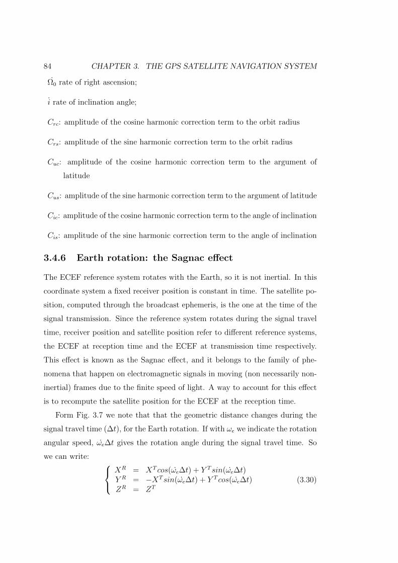
84 CHAPTER 3. THE GPS SATELLITE NAVIGATION SYSTEM
Ω0 rate of right ascension;
i rate of inclination angle;
Crc: amplitude of the cosine harmonic correction term to the orbit radius
Crs: amplitude of the sine harmonic correction term to the orbit radius
Cuc: amplitude of the cosine harmonic correction term to the argument of
latitude
Cus: amplitude of the sine harmonic correction term to the argument of latitude
Cic: amplitude of the cosine harmonic correction term to the angle of inclination
Cis: amplitude of the sine harmonic correction term to the angle of inclination
3.4.6 Earth rotation: the Sagnac effect
The ECEF reference system rotates with the Earth, so it is not inertial. In this
coordinate system a fixed receiver position is constant in time. The satellite po-
sition, computed through the broadcast ephemeris, is the one at the time of the
signal transmission. Since the reference system rotates during the signal travel
time, receiver position and satellite position refer to different reference systems,
the ECEF at reception time and the ECEF at transmission time respectively.
This effect is known as the Sagnac effect, and it belongs to the family of phe-
nomena that happen on electromagnetic signals in moving (non necessarily non-
inertial) frames due to the finite speed of light. A way to account for this effect
is to recompute the satellite position for the ECEF at the reception time.
Form Fig. 3.7 we note that that the geometric distance changes during the
signal travel time (∆t), for the Earth rotation. If with ωe we indicate the rotation
angular speed, ωe∆t gives the rotation angle during the signal travel time. So
we can write: XR = XT cos(ωe∆t) + Y T sin(ωe∆t)Y R = −XT sin(ωe∆t) + Y T cos(ωe∆t)ZR = ZT
(3.30)
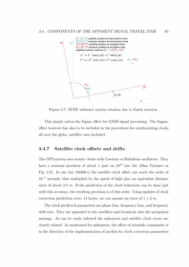
3.4. COMPONENTS OF THE APPARENT SIGNAL TRAVEL-TIME 85
Figure 3.7: ECEF reference system rotation due to Earth rotation.
This simply solves the Signac effect for GNSS signal processing. The Sagnac
effect however has also to be included in the procedures for synchronizing clocks
all over the globe, satellite ones included.
3.4.7 Satellite clock offsets and drifts
The GPS system uses atomic clocks with Caesium or Rubidium oscillators. They
have a nominal precision of about 1 part on 1013 (see the Allan Variance in
Fig. 3.2). In one day (86400 s) the satellite clock offset can reach the order of
10−7 seconds, that multiplied by the speed of light give an equivalent distance
error of about 2.5 m. If the prediction of the clock behaviour can be done just
with this accuracy, the resulting precision is of this order. Using updates of clock
correction prediction every 12 hours, we can assume an error of 1÷ 2 m.
The clock predicted parameters are phase bias, frequency bias, and frequency
drift rate. They are uploaded to the satellites and broadcast into the navigation
message. As can be easily inferred the ephemeris and satellite clock errors are
closely related. As mentioned for ephemeris, the effort of scientific community is
in the direction of the implementation of models for clock correction parameters
86 CHAPTER 3. THE GPS SATELLITE NAVIGATION SYSTEM
prediction with increasing accuracy. In real time Ultra-Rapid ephemeris there are
also clock correction parameters, predicted with a nominal accuracy of 1.5 ns,
i.e. 0.45 m. The best accuracy can be gained with the delayed service, after
12÷ 18 days, that is 20 ps equivalent to 6mm
Residual satellite clock errors are the same in all measurement involving the
same satellite, including P-code, C/A code and carrier phase, and can be removed
when differential techniques are applicable.
3.4.8 Receiver clock errors
GPS receiver commonly use cheap crystal clocks, which are much less accurate
than satellite clocks (see the Allan Variance in Fig. 3.2). The quartz receiver clock
is however more stable than satellite atomic ones, for instantaneous observations.
Therefore the quartz clocks are very suited for positioning purposes that require
high stability for very short periods (tens of nanoseconds), that go from the
transmission instant to the reception one.
The receiver clock offset, including receiver and satellite instrumental biases,
should be considered as a constant for all observations regarding different satel-
lites on view at the same instant. If atmospheric effects are neglected the problem
has a simple solution. In the positioning problem, in fact, it becomes an unknown
in addition to the three receiver coordinates and can be computed by solving a
system of equations for the pseudorange, ρij, that, neglecting atmospheric effects
and all other error sources (orbital, instrumental etc.) can be written as:
ρij(Tj, f) =√
[X i(T ij )−Xj(Tj)]2 + [Y i(T ij )− Yj(Tj)]2 + [Zi(T ij )− Zj(Tj)]2
+c [εrj(Tj)− εis(T ij )](3.31)
with X, Y , Z, coordinates and εr clock offset of satellite, if with apex i, and
receiver, if with subscript j. Clearly four (non aligned) observations guarantee
to solve the problem. A receiver clock error thus can be much larger than satel-
lite clock errors: however theoretically it can be removed by making differences
between observations relative to different satellites.
3.4. COMPONENTS OF THE APPARENT SIGNAL TRAVEL-TIME 87
Of course in atmospheric sounding the problem is more complex, as Eq. (3.31)
must be completed with atmospheric effects, that are unknown in addition to
receiver clock errors, and the valuation through differential observations is no
more straightforward.
Clock stability depends critically on the type of oscillator in use. A crystal
oscillator is an electronic oscillator circuit that uses the mechanical resonance
of a vibrating crystal of piezoelectric material to create an electrical signal with
a very precise frequency. Iit is thus possible to obtain stabilised frequencies,
that, however are influenced by temperature. In order to cope with temperature
instabilities various forms of compensation are used, from analog compensation
(TCXO) to stabilisation of the temperature through a crystal oven (OCXO)5.
OCXO are the most stable oscillators, as they are actively stabilised in temper-
ature. TCXO on the contrary has a sort of feedback mechanism that realigns
frequencies when, due to temperature variations, they jump beyond predeter-
mined thresholds. In Fig. 3.8 there are two example measurements of GPS
signals we have processed from two receivers of the GPS network of the Regione
Toscana, mounting these two different kinds of oscillators. We have used differ-
ential measurements with a time lag of ∆t = 1 s of pseudorange ρ and satellite
distance from the receiver R, in order to eliminate (at a first order) slow varying
contributes (due to atmosphere, antennas, biases, etc.). We have also computed
a ionospheric-free signal and from this a “total” bias B less the tropospheric
delay, c τTrop, that we expected to possess a short term stability. B is the sum of
three terms, the first consists of known parameters, namely the interfrequency
bias B2−1 and the ratio of the square frequencies, γ; the second is the clock
bias, bc, and the third is the signal processing bias, b(f2), that are unknown.
We can easily observe the dramatic difference in stability of the two oscillators,
and the large realignment jumps of 100ns (equivalent to about 30m) for TCXO
measurements, that brings to a very unstable bias, much greater than precision
5TCXO stays for Temperature Controlled Crystal Oscillator; OCXO stays for Oven Con-trolled Crystal Oscillator (being “XO” an old acronym for “crystal oscillator”).
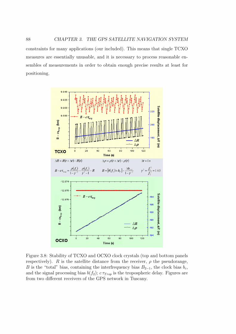
88 CHAPTER 3. THE GPS SATELLITE NAVIGATION SYSTEM
constraints for many applications (our included). This means that single TCXO
measures are essentially unusable, and it is necessary to process reasonable en-
sembles of measurements in order to obtain enough precise results at least for
positioning.
Figure 3.8: Stability of TCXO and OCXO clock crystals (top and bottom panelsrespectively). R is the satellite distance from the receiver, ρ the pseudorange,B is the “total” bias, containing the interfrequency bias B2−1, the clock bias bc,and the signal processing bias b(f2); c τTrop is the tropospheric delay. Figures arefrom two different receivers of the GPS network in Tuscany.
3.4. COMPONENTS OF THE APPARENT SIGNAL TRAVEL-TIME 89
3.4.9 Multipath
If the GPS signal reaches the receiver antenna after reflections from obstacles,
or from the Earth surface, we have the “multipath” phenomenon. The presence
of indirect signals, that arrive later than direct ones and interfere with them,
causes waveform distortion but also phase distortion. Multipath errors affect
both carrier phase and pseudorange measurements, but the effects in the carrier
phase measurement is limited to a quarter of a cycle and in the pseudorange mea-
surements can reach several tens of metres (in C/A code measurements). The
problem is that the error on pseudorange measurements can degrade the ambi-
guity resolution process required for using carrier phase measurements. Limiting
the analysis to the effects on carrier phase the error derived from multipath is
maximum when vectors of the direct and reflected signals are perpendicular. It
does not exist a completely safe mitigation technique for the multipath effects,
but a series of efficient and commonly used methods, primarily based on receiver
hardware solutions. The use of differential GPS cannot reduce the multipath
effects. Multipath effects can be detected if dual frequency observation are avail-
able (after compensation for ionospheric effects). The best ways to mitigate
multipath effects are:
• to choose an installation site with a limited number of near potential re-
flecting objects;
• to use a groundplane antenna (i.e. chock ring) able to attenuate signal
reflected from the ground;
• to use a directive antenna array with many directive patterns simultane-
ously operative and able to adapting to changing satellites geometry;
• to use an hardware (antenna gain) or software (signal processing) selected
“cutoff” angle (i.e. minimum desired elevation angle) to eliminate mea-
surements with low satellite elevation angles which have higher probability
to generate multipath;
90 CHAPTER 3. THE GPS SATELLITE NAVIGATION SYSTEM
• to use a polarised antenna able to match the polarisation of the GPS signal
(i.e., right hand) but mitigating in this case only single reflection or odd
number of them;
• to observe the signal for a longer time than strictly needed, in order to
detect sudden changes caused by multipath (only for fixed stations);
• to use decoding techniques based on narrow correlation of the receiver that
allow to suppress automatically signals delayed by more than 1.5 chips (a
chip correspond to 1 pulse: about 1µs for the C/A-code and about 100ns
for the P-code);
• to analyse the shape of the correlation function.
Other methods exist but they will not be analysed in this work. Is is sufficient
to mention that receivers with chock ring antenna have been chosen for all the
used fixed station and they have been installed over roofs of buildings and far
from sources of reflections.
3.4.10 Additional error sources
In addition to the errors discussed in the previous sections, there are a number
of additional error sources whose effects are generally of secondary importance.
The main contributions of these secondary sources can be however corrected in
order to minimise the further uncertainties they can introduce. The variation
of the antenna centres is one of these. This effect is well known and it has a
straightforward impact on the variation of the signal travel length. Another well
known source is due to tidal effects, namely the Earth tide and the ocean loading
effects. Inland water loading is another one (e.g. cf. [44]). If not corrected they
can contribute up to a few mm of errors or even more6, that for atmospheric
applications are still relevant. When corrected, thanks to well calibrated public
models, their contribution to error is essentially negligible.
6In some regions of the planet tidal effects can reach tens of centimetres.
3.5. OTHER GNSS SYSTEMS 91
From what shown up to now in this chapter, we can understand how sin-
gle quasi real-time measurements of GPS delays have errors at least of a few
centimetres. However approaches based on simultaneous processing of several
observations, better if involving one or more reference fixed stations with precise
receivers, can improve the accuracy up to an order of magnitude.
3.5 Other GNSS systems
Satellite navigation has become a matter of main interest for several countries.
A number of systems with global or local navigation capability are already op-
erational or on experimental stage. In the following we give some details on two
systems of main interest for their characteristics and capability of integration
with GPS: the Russian GLONASS and the European GALILEO.
3.5.1 GLONASS
GLONASS (GLObal NAvigation Satellite System) is an alternative to the US
GPS system. As GPS, it is composed by two main services: the military one
and the civil one, with civil services and applications quality-degraded. The full
constellation is composed by 24 satellites (excluding spare ones) equally spaced
over 3 orbital planes. Satellites orbit are near circular at altitude of 19100 km
over the Earth surface. Orbital planes are inclined 64.8 on the equatorial plane.
Revolution time is 11 hours and 15 minutes.
The ground control stations of the GLONASS are maintained only in the
territory of the former Soviet Union, thus limiting the global coverage capability
of the system. The satellite coverage of GLONASS is greater at northern lati-
tudes, where GPS system has minimum coverage. In the signal transmission the
GLONASS system uses a spread spectrum technology. The signal are right-hand
circularly polarized and the modulation type is the BPSK (Binary Phase Shift
Keying). The code is the same for all the satellites, but each satellite transmit in
a different frequency using a total of 25-channels to realize a Frequency Division
92 CHAPTER 3. THE GPS SATELLITE NAVIGATION SYSTEM
Multiple Access (FDMA)7.
Two main frequencies are used for navigation: L1 (1602.0 MHz) and L2
(1246 MHz). The central frequency relative to each satellite carrier can be
obtained as follow:
L1 = 1602 + n× 0.5625MHz
L2 = 1246 + n× 0.4375MHz (3.32)
with n = −12, ...0, ..., 12.
GLONASS satellites transmit two types of signals: a standard precision (SP)
signal and a so called “obfuscated” high precision (HP) signal. The chipping
rates for the HP and SP codes are 5.11 and 0.511 Mbps, respectively. The HP
signal is broadcast in phase quadrature with the SP signal, has a ten time larger
bandwidth and is available only for authorised users. As with GPS also with
GLONASS it is possible to make phase measurements through carrier signals.
The navigation message (50 bps) contains the parameters for computing spa-
tial and temporal coordinates of each satellite. The combination of measurements
and navigation messages allows to determine the position coordinates, the speed
vectors and the time of the receiver.
GLONASS has been operational since 1982. Its operational history is linked
the URSS political and economic events. The first modernisation plan is the
GLONASS-M from 2003; the second modernization plan, GLONASS-K, is be-
ing implemented from 2011: the first GLONASS-K satellite has already been
launched, on the 26th of February 2011. At present civilian GLONASS is a bit
less accurate than GPS, but the GLONASS-K system will double the accuracy
of the previous one.
3.5.2 Galileo
GALILEO is a joint initiative of ESA and EC. It is a global satellite navigation
system designed to provide a multimodal service, in different domains. It is
7Satellites placed at the antipodes of an orbit use the same frequency: as they are neversimultaneously visible, there is no possibility of signal source ambiguity.
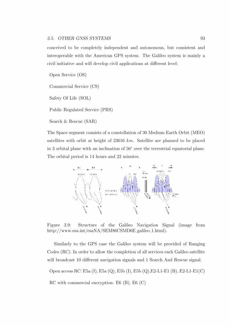
3.5. OTHER GNSS SYSTEMS 93
conceived to be completely independent and autonomous, but consistent and
interoperable with the American GPS system. The Galileo system is mainly a
civil initiative and will develop civil applications at different level:
Open Service (OS)
Commercial Service (CS)
Safety Of Life (SOL)
Public Regulated Service (PRS)
Search & Rescue (SAR)
The Space segment consists of a constellation of 30 Medium Earth Orbit (MEO)
satellites with orbit at height of 23616 km. Satellite are planned to be placed
in 3 orbital plane with an inclination of 56 over the terrestrial equatorial plane.
The orbital period is 14 hours and 22 minutes.
Figure 3.9: Structure of the Galileo Navigation Signal (image fromhttp://www.esa.int/esaNA/SEM86CSMD6E galileo 1.html).
Similarly to the GPS case the Galileo system will be provided of Ranging
Codes (RC). In order to allow the completion of all services each Galileo satellite
will broadcast 10 different navigation signals and 1 Search And Rescue signal.
Open access RC: E5a (I), E5a (Q), E5b (I), E5b (Q),E2-L1-E1 (B), E2-L1-E1(C)
RC with commercial encryption: E6 (B), E6 (C)
94 CHAPTER 3. THE GPS SATELLITE NAVIGATION SYSTEM
RC with governmental encryption: E6 (A), E2-L1-E1(A)
The Galileo signal bands will be:
1164− 1215 MHz
1260− 1300 MHz
1559− 1591 MHz
Different codes for different satellite reception is possible using CDMA. Different
signals are broadcast on the in-phase (I) and in quadrature (Q) channels and,
in the case of the 1164÷ 1215 MHz, different signals are provided in the upper
(E5b) and lower (E5a) part of the band.
The first testing platforms, GIOVE-A and GIOVE-B have been launched in
2005 and in 2008 respectively. In a second moment four IOV (In Orbit Validation)
Galileo satellites will be launched starting from April 2011. These satellites will
be very similar to the final satellite system configuration. The Full Operational
Capability will be completed with the launch of 30 operational satellites.
3.5.3 Complementarity and interoperability
The fundamental frequency of both GPS and GLONASS and Galileo system is
the same: f0 = 10.23 MHz. This simplifies the design and construction of
receivers that can detect all signals coming from all satellite systems. An advan-
tage of simultaneous processing of several observations, especially for retrieving
atmospheric parameters, is that such data redundancy contributes to better re-
move oscillation, drift, biases etc., and generally a large number of satellite on
view improve the measurement accuracy. As a consequence the perspectives for
GNSS “non-native” applications, such as the atmospheric one, so demanding in
terms of accuracy and number of observations, become more and more interest-
ing. The future development of GLONASS, GPS and Galileo are on line with
these expectations, not only for the upgrading on single satellite signals, but also
3.5. OTHER GNSS SYSTEMS 95
because they are planned to ensure the interoperability among the various sys-
tems, for example foreseeing signals sharing by satellites belonging to different
systems.
This trend involves also other global navigation systems, extending also to
systems under development, as the Chinese Beidou and the Indian IRNSS sys-
tems, conceived as regional systems but on the way to be extended towards a
global coverage.
96 CHAPTER 3. THE GPS SATELLITE NAVIGATION SYSTEM
Chapter 4
Retrieval of atmospheric profiles
4.1 Classical approaches for GNSS Water Vapour
retrieval
In the present chapter we will assume that we have a GPS (or more generally a
GNSS) precision signal delay already “cleaned” from ionospheric effects, various
biases and the distance between the receiver and the satellite. The delay δl = cδt,
thus measured as a distance, will be only due to the neutral atmospheric effects,
that is mainly (around 90%) due to the troposphere.
In § 2.2 we have seen that the refractive index for the neutral component of
the atmosphere can be expressed as:
n = n(z) = n (Pd(z), T (z), e(z)) (4.1)
It is useful to introduce N defined as N = n − 1, that, from Eq. (2.42), and
neglecting the contribution for non ideal-gas behaviours (i.e. assuming Zd '
Zw ' 1), can be written as:
N = c1PdT
+[c2 +
c3
T
] eT
(4.2)
From what discussed in § 2.3, the signal delay, δl, will be:
δl =
∫L
Nds (4.3)
being L the ray path, that we assume coincident with the straight line connecting
the satellite to the receiver, committing a negligible error, as shown in § 2.3.3.
97
98 CHAPTER 4. RETRIEVAL OF ATMOSPHERIC PROFILES
Thanks to the integral mean value theorem1, from δl we can immediately
obtain an average measure of N along L. If we want to get more than this from
GNSS delays, we have to include additional information and/or assumptions.
A method that can be considered a sort of “classical way” to proceed in order
to extract at least an average estimation of water vapour (i.e. of e) or related
quantities, will be illustrated in the following of this section. The aim of such
method is to retrieve values of precipitable water at the receiver coordinates,
using GNSS delays and local in-situ pressure and temperature measurements.
Precipitable water is the depth of the amount of water in a column of the at-
mosphere, as if all the water in that column were precipitated as rain2. The
relevance of the method lays on the fact that it is rather simple, that in addi-
tion to GNSS measurements it needs just basic atmospheric parameters as given
by common meteorological stations (as normally installed close to GNSS fixed
stations) and that it produces a parameter of main meteorological interest, as
precipitable water is. For this reasons it is at the basis of a number of works
on GNSS atmospheric applications, whose differences are more on preprocessing
methods to obtain δl, than on the core of the precipitable water retrieval. The
main limitations are in some assumptions that are adopted and that will be com-
mented step by step, and in the information that is virtually wasted and that
has been the primary reason from which the present work has been originated.
The basic idea is to partition the total atmospheric delay into a large quantity
which depends only on the total ground pressure, called the “hydrostatic delay”,
and a smaller quantity which is a function of water vapour distribution and that
1The integral mean value theorem states that, if f : [a, b] → R is a continuous function onthe closed interval [a, b], and differentiable on the open interval ]a, b[, where a < b, then thereexists some c ∈]a, b[ such that:
f(c) =1
b− a
∫ b
a
f(x)dx .
2Generally water in an atmospheric column can be present as water vapour, liquid waterand ice crystals. The GNSS signal delay however depends on vapour and few on liquid wateror ice. Thus we will assume contributions to the total water other than vapour to be negligible,knowing that this is not always verified.
4.1. CLASSICAL APPROACHES FOR GNSS WV RETRIEVAL 99
is called the “wet delay” ([35]; [13]).
Let us consider only zenith observations of the delays, using ZHD for the
zenith hydrostatic delay and ZWD for the zenith wet delay.
A semi-empirical relationship between ZHD and the total pressure, Ps at the
Earth’s surface, can be assumed, as in [17]:
∆L0h = ZHD = (2.2779± 0.0024)
Psf(λ,H)
(4.4)
where ZHD is in millimetres, Ps in millibars, and:
f(λ,H) = 1− 0.00266 cos(2λ)− 0.00028H (4.5)
accounts for the variation in gravitational acceleration with the latitude λ and
the height H, expressed in kilometres. The hydrostatic delay in Eq. (4.4) is not
exactly the “dry delay”, as it is given in terms of the total pressure and not on
the partial pressure of dry air. We could say that ZHD is made by all the parts of
N that depend on P/T , included the non-polar contribution from water vapour,
the largest contribution to the hydrostatic delay remaining however that of the
dry air. Wet delay consequently refers to the component produced mainly by
the atmospheric water vapour, due to the dipole component of its refractivity.
Then ZWD is given by:
∆L0w = ZWD = c′2
∫e
Tdz + c3
∫e
T 2dz (4.6)
where c′2 = (17±10) ·10−6Kmbar−1 is different from c2 in Eq. (2.42) (because of
the part included in the ZHD), while c3 is the same (cf. [13]. Eq. (4.6) is usually
approximated to:
∆L0w = C
∫e
T 2dz (4.7)
with C = 0.382± 0.004K2mbar−1
Now we have a relationship between ZHD and Ps that is considered fairly
good, while GNSS data are necessary to evaluate ZWD, for which no accurate
relationship with solely ground parameters is achievable.
100 CHAPTER 4. RETRIEVAL OF ATMOSPHERIC PROFILES
In order to be able to link a GNSS observation of tropospheric delay to ZHD
and ZWD, we need to map delays along paths with arbitrary elevation angles
into zenith delays. Mapping functions are summoned at this purpose. The total
delay for a path with an elevation angle α 3, is computed from the hydrostatic
and wet zenith delays via:
∆L = ∆L0hMh(α) + ∆L0
wMw(α) (4.8)
where Mh(α) and Mw(α) are the hydrostatic and wet mapping functions respec-
tively. Various forms have been proposed for the wet and hydrostatic mapping
functions (e.g. Chao; [13]). These functions differ in the number of meteoro-
logical parameters that are incorporated, some simply referring to geographical
features, other including meteo/climatic ones. Because hydrostatic and wet map-
ping functions are similar above elevation angles of 15 and GPS observations
at lower elevations are rarely used, they are jointly estimated, grouping the two
delays together ([41]). Nearly all of the mapping functions that have been sug-
gested in the literature assume no azimuth variation in path delay, but it is
known that the assumption of azimuth symmetry may cause significant errors
(some centimetres) when the local troposphere has large horizontal temperature,
pressure, or humidity gradients, as usually come with strong frontal weather
systems ([12]).
Now, if we assume to have found an expression for the mapping functions that
satisfy our needs, we still need to derive an approximate relationship between
the vertically integrated water vapour (IWV) and an observed zenith wet delay.
We can then introduce the weighted “mean temperature” of the atmosphere, Tm,
defined by (cf. [13]):
Tm =
∫eTdz∫
eT 2 dz
(4.9)
Combining Eq. (4.6) with Eq. (4.9), and the equation of state for water vapour
we obtain:
IWV =
∫ρwdz ' k∆L0
w (4.10)
3Note that hereafter we use α for indicating what in Fig. 2.7 was the complementary of α1.
4.1. CLASSICAL APPROACHES FOR GNSS WV RETRIEVAL 101
where ∆L0w is the zenith wet delay, and k is given by (cf. [4]):
1/k =
(c3
Tm+ c′2
)Rw (4.11)
where Rw is the specific gas constant for water vapour (see § 1.2.1). It is IWV
that sometimes is stated as the height of an equivalent column of liquid water,
i.e. the precipitable water (PW). Numerically, the IWV is just the product of
PW and ρl, the latter being the density of liquid water. PW as ZWD have units
of length and we have:
PW =k
ρlZWD (4.12)
From Eq. (4.11) we observe that an estimation of Tm is necessary for re-
trieving PW. This could be done, for example, by statistical analysis of a large
number of radiosonde profiles, in order to obtain a model of Tm “tuned” to a
specific area and season. This gives very rough estimation of Tm and a more
reliable approach can be to use operational meteorological models to predict its
actual value. Alternatively Tm can be estimated on the basis of the observed
ground temperature, using suitable atmospheric profiles calibrated to the mea-
surement point(s). A number of different solutions have been tried for this issue
(e.g. cf. [4]), and for some of them the error on the final estimation of IWV is
claimed to be a few percents. However these error estimates are generally the re-
sult of posterior validations, made on more or less averaged quantities, while the
number of assumptions on the atmospheric structure, and the equation simplifi-
cations we have previously listed (plus all the uncertainties in the tropospheric
delay estimation), makes error on single measurements realistically much higher
and also very variable and little predictable.
The lack of knowledge of reliable error on single measurements, related to the
specific measurement conditions, is one of the weak point of all approaches be-
longing to the “family” of the described one. Another weak point is in the forcing
of the problem solution to a zenith integrated estimation of average atmospheric
parameters. On one side this implies assuming symmetries and homogeneities
for the atmosphere that generally are not verified. On the other side it prevents
102 CHAPTER 4. RETRIEVAL OF ATMOSPHERIC PROFILES
the exploitation of the horizontal and vertical information contained in the nu-
merous simultaneous GNSS observations from different satellites and different
stations, whose interest will increase more and more in the future thanks to the
increasing number of operational platforms, satellite constellations and ground
stations, most of the latter installed for different purposes , but that can become
a precious resource also in atmospheric science.
This high number of different profiles could in principle open the possibility to
a tomographic retrieval of the main atmospheric parameters (the one N depends
on). In the following section we will analyse which are the limits of applicability
of the classical tomographic approach with respect to our issue, in order to
propose and test an alternative probabilistic approach, that will be described in
the second part of the present chapter.
4.2 Classical tomographic recontruction prob-
lem
The intensity I of a signal crossing a layer dl of absorbent material is reduced
by an amount dI proportional to the product Idl 4, that is:
dI = −κIdl (4.13)
where κ is the linear absorption coefficient of the medium. By integrating
Eq. (4.13) along the path L, followed by the signal inside the absorbent medium,
we obtain:
IL = I0 exp
(−∫L
κ dl
)(4.14)
which reduces to the law of Beer-Lambert, and simplifies in an exponential decay
for the intensity, if the absorption coefficient remains constant along the entire
path. Therefore, if a signal of known intensity I0 is sent through an absorbent
medium, the measure of the emerging intensity IL, allows to immediately retrieve
4This is true within the limit of validity of linear absorption.
4.2. CLASSICAL TOMOGRAPHIC RECONTRUCTION PROBLEM 103
the integrated absorption coefficient:∫L
κ dl = lnI0
IL(4.15)
The basic data for a tomographic reconstruction are just a set of values ex-
pressing line integrals of the type (4.15), characterising the features of a medium.
Signals can be radio waves, visible light, beam of X-rays or neutrons, acous-
tic waves etc., and the basic integrated feature has not to be necessarily the
absorption coefficient, thus it can be something not necessarily derived from
measurements of absorption. In this work, for instance, we deal with integrated
path delays of MW L-band radiation, and the feature of interest are “local”
delays, i.e. locally averaged refractive indexes n, from which retrieving basic
thermodynamic parameters for the troposphere, namely partial pressure of the
dry gas mixture, partial pressure of water vapour, and temperature (or some
derived quantities).
In the following we will denote by n instead of κ a general feature to be
determined. This is not only for similarity to our problem, but also and primarily
to avoid confusion with the conjugate variable of the spatial coordinates (x, y, z),
typically denoted by (kx, ky, kz).
With these notation, the general problem of tomography is to reconstruct the
spatial distribution of the feature n(x, y, z) characterising a medium in a certain
volume V from a set of line integrals of the form (4.15) along different paths L.
For simplicity we will consider a two-dimensional problem (but results can be
directly generalised to the three dimensional case). The medium thus extends
in the plane identified by the Cartesian reference system (x, z). We suppose
to be able to measures integrated quantities along straight lines Lα(s), with α
indicating the elevation angle with respect to the x axis and s a coordinate along
the direction perpendicular to the lines themselves, as shown in Fig. 4.1.
The following function:
f(α, s) =
∫Lα(s)
n(x, z)dl (4.16)
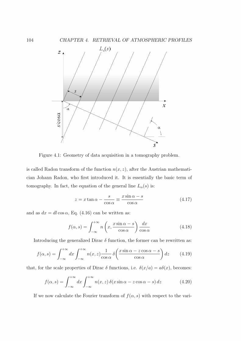
104 CHAPTER 4. RETRIEVAL OF ATMOSPHERIC PROFILES
Figure 4.1: Geometry of data acquisition in a tomography problem.
is called Radon transform of the function n(x, z), after the Austrian mathemati-
cian Johann Radon, who first introduced it. It is essentially the basic term of
tomography. In fact, the equation of the general line Lα(s) is:
z = x tanα− s
cosα≡ x sinα− s
cosα(4.17)
and as dx = dl cosα, Eq. (4.16) can be written as:
f(α, s) =
∫ +∞
−∞n
(x,x sinα− s
cosα
)dx
cosα(4.18)
Introducing the generalized Dirac δ function, the former can be rewritten as:
f(α, s) =
∫ +∞
−∞dx
∫ +∞
−∞n(x, z)
1
cosαδ
(x sinα− z cosα− s
cosα
)dz (4.19)
that, for the scale properties of Dirac δ functions, i.e. δ(x/a) = aδ(x), becomes:
f(α, s) =
∫ +∞
−∞dx
∫ +∞
−∞n(x, z) δ(x sinα− z cosα− s) dz (4.20)
If we now calculate the Fourier transform of f(α, s) with respect to the vari-
4.2. CLASSICAL TOMOGRAPHIC RECONTRUCTION PROBLEM 105
able s, we obtain for the main property of the Dirac δ:
f(α, ks) ≡1√2π
∫ +∞
−∞f(α, s) exp(−ikss)ds
=1√2π
∫∫ +∞
−∞n(x, z) exp(−ixks sinα + izks cosα)dxdz
(4.21)
This expression, apart for a multiplication factor, is clearly the Fourier trans-
form of n(x, z) evaluated at the point of the conjugate space
(kx = ks sinα , kz = −ks cosα) :
f(α, ks) =√
2π n(ks sinα,−ks cosα) (4.22)
For a given α angle and varying ks, these points lay on the line
kx = −kz tanα of the conjugate space (kx, kz). This definitely solves the prob-
lem of reconstructing n(x, z), just anti-transforming n computed from f through
Eq. (4.22).
In real problems continuous features give place to discrete sampling, and
consequently Fourier integrals become discrete Fourier transforms. The Nyquist-
Shannon theorem (cf. [37]) assesses that a signal s(t) with a limited band fM
can be univocally reconstructed through samples s(n∆t), with (n ∈ Z), taken at
frequency fs = 1∆t
if fs > 2fM . We can also interpret such theorem as establishing
the relationship between sampling frequencies and domain dimensions in Fourier
conjugate spaces. Coming back to our problem, thanks to the formal symmetry
between Fourier transforms and anti-transforms, the Nyquist-Shannon theorem
gives us the relationship between spatial resolutions (∆x , ∆z) and the amplitude
of the frequency domains (kx, kz), that in turn is linked to the range dimensions
for ks and for the angle α 5.
There are two things that consequently comes out from the previous analysis,
that says that classical tomography is feasible if:
5For the same symmetry reasons the intervals (∆kx,∆kz) are linked to the dimension in(x , z) of the medium to be sounded.
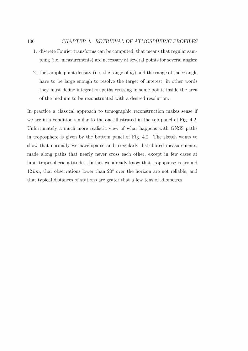
106 CHAPTER 4. RETRIEVAL OF ATMOSPHERIC PROFILES
1. discrete Fourier transforms can be computed, that means that regular sam-
pling (i.e. measurements) are necessary at several points for several angles;
2. the sample point density (i.e. the range of ks) and the range of the α angle
have to be large enough to resolve the target of interest, in other words
they must define integration paths crossing in some points inside the area
of the medium to be reconstructed with a desired resolution.
In practice a classical approach to tomographic reconstruction makes sense if
we are in a condition similar to the one illustrated in the top panel of Fig. 4.2.
Unfortunately a much more realistic view of what happens with GNSS paths
in troposphere is given by the bottom panel of Fig. 4.2. The sketch wants to
show that normally we have sparse and irregularly distributed measurements,
made along paths that nearly never cross each other, except in few cases at
limit tropospheric altitudes. In fact we already know that tropopause is around
12 km, that observations lower than 20 over the horizon are not reliable, and
that typical distances of stations are grater that a few tens of kilometres.
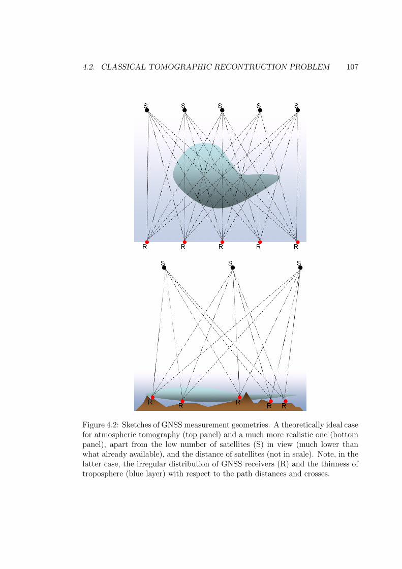
4.2. CLASSICAL TOMOGRAPHIC RECONTRUCTION PROBLEM 107
Figure 4.2: Sketches of GNSS measurement geometries. A theoretically ideal casefor atmospheric tomography (top panel) and a much more realistic one (bottompanel), apart from the low number of satellites (S) in view (much lower thanwhat already available), and the distance of satellites (not in scale). Note, in thelatter case, the irregular distribution of GNSS receivers (R) and the thinness oftroposphere (blue layer) with respect to the path distances and crosses.
108 CHAPTER 4. RETRIEVAL OF ATMOSPHERIC PROFILES
We could argue that the irregular distribution of receivers could be overcome,
assuming a regular network of virtual receivers whose measurements are given by
some interpolation techniques of data from real receivers. If Fourier series are the
target, they could own some properties that facilitate the issue: some suggestions
could be searched in approaches like, for example, the one known as the Lomb
method for spectral analyses of irregularly sampled data (cf. [26]). However
interpolation methods bring always additional errors, that in our case should be
carefully managed. Furthermore this would not solve the problem of scarcity
of crossing profiles: since we are particularly interested in water vapour, it is
the low troposphere that must be resolved with highest accuracy, exactly where
we have no crossing paths. At the end we need more resolution (both vertical
and horizontal) where we have less information from a classical tomographic
point of view. This is equivalent to saying that the problem appears strongly
underconstrained, and the approach that seems more natural is the probabilistic
(Bayesian) one.
4.3 A probabilistic approach to atmospheric to-
mography
Assume that we have a set of state vectors for the profiles of the target parame-
ters, and assume that this set is complete, meaning that it contains all possible
states of the target parameters. This means also that such set forms an ideal
a priori knowledge of the target parameters. it will be very dense to be easily
expressed in terms of a probability density function for each target parameter6.
Now let us imagine to have o set of measurements of observables depending
on some of the target parameters in a known functional form, which can be
assumed deterministic7. Each measurement can be considered as a constraint
6A more realistic view is that we will have a large number of possible values for the targetparameters, such that this set of values can be considered representative, meaning that itreasonably represents our a priori knowledge, and that possibly is dense enough to easily allowits expression in terms of probability density functions.
7This equivalently means that the models that link the target parameters to the observableshave negligible errors. If rigorously speaking this is not the case, we can imagine to cope with
4.3. A PROBABILISTIC APPROACH TO ATM. TOMOGRAPHY 109
with a tolerance given by its uncertainty8 and it allows us to select, from our
a priori dataset, only “state vectors” that satisfy all the available constraints,
within to their tolerance.
So doing we obtain a new dataset of all possible state vectors, given the
available measurements. The best set of target parameters is thus defined by the
most probable state vector, and uncertainties are defined by the new probability
density function for each target parameter (around its best value).
We now want to formalise these concepts according to our specific goals and
we will do it gradually, starting from the simplified case of parameter retrieval in
a one dimensional (1D) problem9, and extending the process to three dimensional
(3D) case.
4.3.1 1D retrievals
The 1D problem can be imagined as the retrieval of some zenith atmospheric
parameters from measurements in a given point of the Earth surface. What de-
scribed in § 4.1 is a special case of the more general 1D problem, where the target
parameter is PW (obtained from the mean value of the wet part of the refrac-
tive index along the zenith path) and the observables are ground total pressure
Ps, ground temperature Ts and the integrated zenith wet delay ZWD, measured
from a fixed GNSS station equipped with meteorological sensors. As the tar-
get parameter is an integrated value along the vertical path, the 1D problem
“collapses” into a 0D one (i.e. a point measurement).
Here instead, we want to address a more general problem of measuring P (z),
T (z) and e(z) from the same measurement configuration (a GNSS station with
meteorological sensors). The observables for us are still Ps and Ts, but instead of
such problem “transferring” a model error (i.e. the probabilistic dependence of an observableon one or more target parameters) into the observable uncertainty.
8If uncertainties are negligible, i.e. the probability density functions for measurements areDirac δ’s, the tolerant constraint “collapses” in a rigid constraint.
9In the following of the present work, the notation ‘nD’ will be always used to identify adimensionality in the real physical space and not in generic geometrical spaces, with n ∈ Nand n ∈ [0, 3].
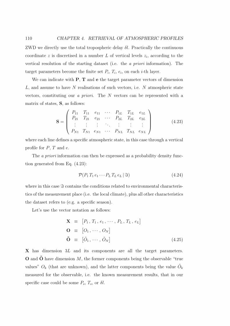
110 CHAPTER 4. RETRIEVAL OF ATMOSPHERIC PROFILES
ZWD we directly use the total tropospheric delay δl. Practically the continuous
coordinate z is discretised in a number L of vertical levels zi, according to the
vertical resolution of the starting dataset (i.e. the a priori information). The
target parameters become the finite set Pi, Ti, ei, on each i-th layer.
We can indicate with P, T and e the target parameter vectors of dimension
L, and assume to have N realisations of such vectors, i.e. N atmospheric state
vectors, constituting our a priori. The N vectors can be represented with a
matrix of states, S, as follows:
S =
P11 T11 e11 · · · P1L T1L e1L
P21 T21 e21 · · · P2L T2L e2L...
......
. . ....
......
PN1 TN1 eN1 · · · PNL TNL eNL
(4.23)
where each line defines a specific atmospheric state, in this case through a vertical
profile for P , T and e.
The a priori information can then be expressed as a probability density func-
tion generated from Eq. (4.23):
P(P1 T1 e1 · · ·PL TL eL | =) (4.24)
where in this case = contains the conditions related to environmental characteris-
tics of the measurement place (i.e. the local climate), plus all other characteristics
the dataset refers to (e.g. a specific season).
Let’s use the vector notation as follows:
X ≡[P1 , T1 , e1 , · · · , PL , TL , eL
]O ≡
[O1 , · · · , ON
]O ≡
[O1 , · · · , ON
](4.25)
X has dimension 3L and its components are all the target parameters.
O and O have dimension M , the former components being the observable “true
values” Ok (that are unknown), and the latter components being the value Ok
measured for the observable, i.e. the known measurement results, that in our
specific case could be some Ps, Ts, or δl.
4.3. A PROBABILISTIC APPROACH TO ATM. TOMOGRAPHY 111
What we assume to know are P(X | =), P(Ok |X=), and P(Ok | Ok =).
P(X | =), is Eq. (4.24), i.e. the a priori information on the target parameters.
P(Ok |X=), is given by the model that links each observable to the target pa-
rameters, and that for us is deterministic through specific functional forms fk,
so that:
P(Ok |X=) = δ (Ok − fk(X)=) (4.26)
P(Ok | Ok =), is the measurement errors. Our goal is to determine P(X | O=).
Thanks to the Bayes’ theorem 10we can write:
P(X | O=) =
B= P(O |X=) · P(X | =)
P(O | =)
=
[∏k
P(Ok |X=)
]· P(X | =)
P(O | =)(4.27)
With ‘B= ’ we have marked exactly where we have used the Bayes’ theorem. The
last (bottom right) term of Eq. (4.27) has been obtained considering that the
result of each measurement is independent on the other measurements, and that
this holds also for measurement prior probabilities.
In order to evaluate the terms into the square roots of Eq. (4.27), we can
observe that:
P(Ok |X=)B= P(X | Ok =)
P(Ok | =)
P(X | =)(4.28)
and that:
P(X | Ok =) =
∫P(XOk | Ok =) dO
=
∫P(Ok | Ok =)P(X |OkOk =) dO (4.29)
10The Bayes’ theorem assesses that:
P(A |B =) =P(B |A=)P(A | =)
P(B | =)
where P (A | =) is the prior probability of A (in the sense that it does not take into accountany information about B); P (A |B =) is the conditional probability of A, given B (sometimesreferred as posterior probability because it depends upon the specified value of B); P (B |A=)is the conditional probability of B, given A, also called the likelihood; P (B | =) is the prior ormarginal probability of B, that can be considered a simple normalising term.
112 CHAPTER 4. RETRIEVAL OF ATMOSPHERIC PROFILES
Now we can further observe that X depends on O only through the true values
O 11. This means that we can write:
P(X |OkOk =) = P(X |Ok =) (4.30)
B= P(Ok |X=)
P(X | =)
P(Ok | =)(4.31)
Substituting Eq. (4.31) into Eq. (4.29) we obtain:
P(X | Ok =) = P(X | =)
∫P(Ok | Ok =)
P(Ok | =)P(Ok |X=) dO
= P(X | =)
∫P(Ok | Ok =)
P(Ok | =)δ (Ok − fk(X)) dO
= P(X | =)P(Ok = fk(X) | Ok =
)P (Ok = fk(X) | =)
(4.32)
Substituting then Eq. (4.32) into Eq. (4.28) we have:
P(Ok |X=) =P(Ok = fk(X) | Ok =
)P (Ok = fk(X) | =)
P(Ok | =) (4.33)
Finally using Eq. (4.33) into Eq. (4.27) we obtain:
P(X | O=) =1
K
[∏k
P(Ok = fk(X) | Ok =
)· P(Ok | =)
]P(X | =) (4.34)
where K is a normalisation term which is given by the expression
K =(P(O | =) ·
∏k P (Ok = fk(X) | =)
), but that can be more easily computed
imposing∫P(X | O=) dX = 1.
In order to reduce computing time, we have assumed for P(Ok | Ok =) a square
shape, that means a constant value for a tolerance range12 and 0 elsewhere:
P(Ok | Ok) =
1/Λ if |Ok − Ok| ≤ Λ/20 otherwise
(4.35)
11This allows to write Eq. (4.30) but of course in general we cannot write P(X | Ok =) =P(X |Ok =) .
12Given the range, the constant value for the square probability function remains definedby the probability normalisation condition, that imposes the integral (or sum over all states)equal to 1.
4.3. A PROBABILISTIC APPROACH TO ATM. TOMOGRAPHY 113
This simplify the implementation of the right part of Eq. (4.34), that has been
done as a direct selection of all and only the states X whose observable values
O fall within the P(O | O=) non-zero domain (i.e. the tolerance range)13. The
relevance of the results that we will show later, is not impacted by this choice,
that however, in real cases, could result too rough (a short discussion on this
issue is postponed to § 5.2).
Compatible values for each target parameter are organised in histograms, in
order to obtain a discrete probability density function. Histogram bins are sized
in order to be about√N , ranging from the variables extremes14. At void bins
(within the range) it is associated the minimum possible probability greater than
0, that is 1/N , for all the void interval. This means that if the same variable has
n0 void bins, at each bin is associated the value 1/(N n0).
Once we have the probability function for each target parameter we have still
not finished the work, unless all parameters can be assumed independent. In
fact if they are independent, the best state vector can be chosen as the vector
of the most probable parameters, and errors are obtained from each probability
functions, around their maxima15. Of course P , T and e cannot be considered
independent variables, nor their values at different layers (especially for adjacent
or near layers). It is thus necessary to move to independent variables.
Generally speaking this can be a complex problem, and it is not assured
that a solution exists that is valid not only locally16, but all over the parameter
domains. A way to address this issue is however the method at the basis of the
computation of the Empirical Orthogonal Functions (EOF, cf. [34]). It starts
from the computation of the covariance matrix of the variables, whose diagonal
13From Eq. (4.34) we understand that we have arbitrarily assumed the term P(Ok | =) noninfluent (as it would be flat) in the range of measurement we deal with.
14This resembles the Poisson noise threshold, in the sense that we want our bin to contain√N “events” on average, with bins more populated than this threshold to be considered very
significant.15This is rigorously true if we assume a unimodal distribution for probability. Bimodal or
multimodal distributions would need specific analyses, but in effect regarding the parameters ofour interest it is reasonably assume that multimodal distribution should come only as artefactsdue to wrong assumptions in the retrieval process.
16The notion of “locality” here refers to a finite small interval of parameter values.

114 CHAPTER 4. RETRIEVAL OF ATMOSPHERIC PROFILES
elements are then cancelled through a matrix diagonalisation, that corresponds
to change (rotating) the starting reference system to a new one, defined by the
eigenvectors of the covariance matrix.
A general definition of the covariance matrix Σ =[σij]
can be given as
follows. Consider the vector:
X =[X1, · · · , X3L
](4.36)
If its entries are random variables, each with finite variance, then the covariance
matrix Σ =[σij]
is the matrix whose (i, j) element is the covariance:
σij = cov(Xi, Xj) = E[(Xi − µi)(Xj − µj)
](4.37)
where µi = E(Xi) is the expected value of the ith entry in the vector X.
In our case X is defined by Eq. (4.25), and the expected values are simply
the mean values of (Pi, Ti, ei).
Regarding the diagonalisation issue, the spectral theorem of linear algebra
assesses that: ∃ V ∈M (R, 3 L × 3 L) , which is orthogonal and satisfies:
Σd = VT ·Σ ·V (4.38)
with Σd diagonal. The eigenvalues gives the variances of the new generalised
variables, with respect to the new reference axes.
By means of a linear transformation Eq. 4.38 allows to transform the S, into
the new matrix Sgen, such that:Sgen = VT · ST
Sgen ∈M (R, N × 3L)(4.39)
We obtain new state vectors in the phase space generated by the (orthogonal)
eigenvectors of Σ. We will name these new state vectors generalised state vectors
(see Fig. 4.3), meaning that they have no more a direct physical sense, because
they do not express physical quantities at given levels (as it is in S), but however
they are linked to them through the simple linear transformation in Eq. (4.39).
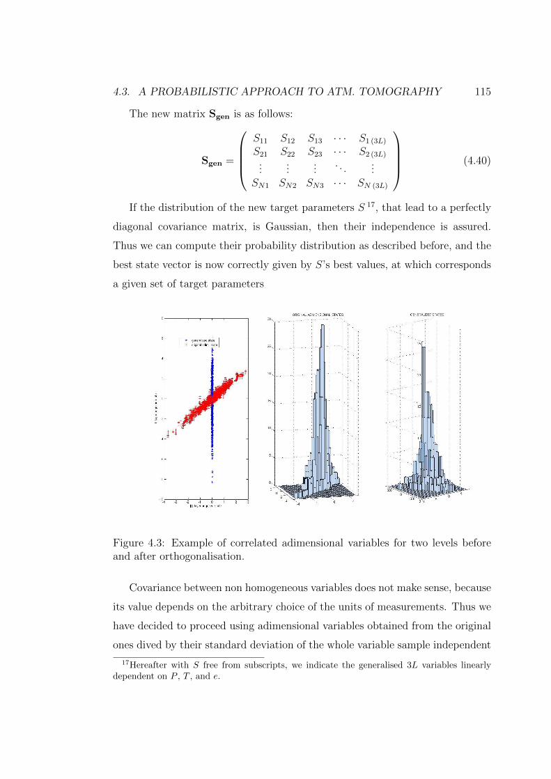
4.3. A PROBABILISTIC APPROACH TO ATM. TOMOGRAPHY 115
The new matrix Sgen is as follows:
Sgen =
S11 S12 S13 · · · S1 (3L)
S21 S22 S23 · · · S2 (3L)...
......
. . ....
SN1 SN2 SN3 · · · SN (3L)
(4.40)
If the distribution of the new target parameters S 17, that lead to a perfectly
diagonal covariance matrix, is Gaussian, then their independence is assured.
Thus we can compute their probability distribution as described before, and the
best state vector is now correctly given by S’s best values, at which corresponds
a given set of target parameters
Figure 4.3: Example of correlated adimensional variables for two levels beforeand after orthogonalisation.
Covariance between non homogeneous variables does not make sense, because
its value depends on the arbitrary choice of the units of measurements. Thus we
have decided to proceed using adimensional variables obtained from the original
ones dived by their standard deviation of the whole variable sample independent
17Hereafter with S free from subscripts, we indicate the generalised 3L variables linearlydependent on P , T , and e.
116 CHAPTER 4. RETRIEVAL OF ATMOSPHERIC PROFILES
on the level. This means, for instance, that each Pi has been divided by the
standard deviation computed on the ensemble (P1, · · · , PL), and the same for Ti
and ei. According to the structure of the matrix in Eq. (4.23), but following the
notation of Eq. (4.37), we have:
Xij → Xij
1
L
√√√√ L∑l=0
σ3l+[1+(j−1) mod 3] 3l+[1+(j−1) mod 3]
−1
(4.41)
where [(j − 1) mod 3] = 0, 1, 2 flags P ’s, T ’s and e’s respectively.
We have to note that the method chosen for the adimensionalisation could
have critical impact one some results18, if we used the EOF (orthogonalisation)
process also to reduce the dimensionality of our problem, neglecting the compo-
nents of the new S variables on the part of phase space mapped through eigen-
vectors corresponding to the lowest eigenvalues (i.e. forcing this phase space
region to the null space). This however has no impact in this work as we have
not reduced the dimensionality of our problem.
4.3.2 Extension to 3D retrievals
The extension to a 3D problem of what discussed in § 4.3.1 is theoretically
straightforward. In fact if we consider to identify the horizontal spatial domain
with a regular mesh, we will have a state vector with the same target parameters
for each node. Our target parameters from 3L will become 3L · M , with M
number of horizontal nodes. The matrix S of Eq. (4.23) will consequently increase
to contain 3L·M columns, but the process to obtain the matrix Sgen of Eq. (4.40)
will obviously remain a matrix diagonalisation. Of course the processing time
will grow up very rapidly with the number of nodes, and an analysis of the true
18Adimensional variables are scale invariant, but the same can be said for any analogousadimensionalisation process with an arbitrary multiplicative factor. Such factors can changethe relative weight of the variable variances in the correlation matrix and so they can changeeigenvalues. If we need EOF also to reduce the dimensionality of the problem, we must beaware of this arbitrariness. Defining variables that are physically homogeneous can solve theproblem. For instance we could express all state vector variables in pressure units. It isstraightforward for the total pressure and for the water vapour partial pressure. Temperatureinstead could be expressed by means of the saturation pressure of water vapour as given inEq. (1.17).
4.4. NUMERICAL EXPERIMENTS 117
dimensionality of the problem will be necessary in order to maintain the number
of significant orthogonal variables into an acceptable limit.
Regarding the constraints in the retrieval process, no difference has to be in-
troduced relatively to measurements of ground parameters. The same is also for
zenith delay. Instead non zenith delay could be processed in order to include the
effects of boundary or crossed cells, in other words the contributions of horizontal
atmospheric gradients. This can be achieved through a proper spatial interpola-
tion for the target parameters, which a given delay measurement depends on. A
simple linear interpolation has been used in our numerical experiment will show
in § 4.4.4, that can be considered more than reasonable along distances of a few
kilometres, due to the “smoothness” of our target atmospheric parameters.
Of course non zenith delays should be compensated through a geometrical
factor for the lengthening of their path due to the inclination. In our numerical
experiments we have worked in a non curved tropospheric geometry and thus
this term is just 1/ sinα, being α the elevation angle .
4.4 Numerical experiments
We have already stated that the principal aim of this work is to assess the feasibil-
ity of a probabilistic approach for retrieving basic atmospheric parameters, and
the advantages in term of information that can be gained by such an approach.
In order to address this issue we have decided to proceed through numerical ex-
periments based on synthetic data, for working in a fully controlled environment.
The reference area is Tuscany and its GNSS network of ground GPS stations19
for precision positioning, mutually connected through the internet network of
Regione Toscana, with an average distant between stations around 25 km.
19Three GPS stations are located and maintained by the LAMMA Consortium(www.lamma.rete.toscana.it), where this work has been developed.
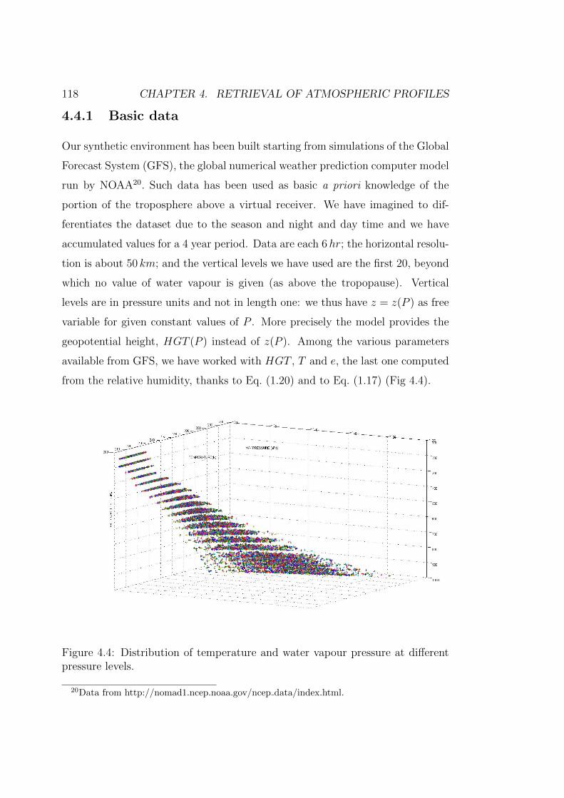
118 CHAPTER 4. RETRIEVAL OF ATMOSPHERIC PROFILES
4.4.1 Basic data
Our synthetic environment has been built starting from simulations of the Global
Forecast System (GFS), the global numerical weather prediction computer model
run by NOAA20. Such data has been used as basic a priori knowledge of the
portion of the troposphere above a virtual receiver. We have imagined to dif-
ferentiates the dataset due to the season and night and day time and we have
accumulated values for a 4 year period. Data are each 6hr; the horizontal resolu-
tion is about 50 km; and the vertical levels we have used are the first 20, beyond
which no value of water vapour is given (as above the tropopause). Vertical
levels are in pressure units and not in length one: we thus have z = z(P ) as free
variable for given constant values of P . More precisely the model provides the
geopotential height, HGT (P ) instead of z(P ). Among the various parameters
available from GFS, we have worked with HGT , T and e, the last one computed
from the relative humidity, thanks to Eq. (1.20) and to Eq. (1.17) (Fig 4.4).
Figure 4.4: Distribution of temperature and water vapour pressure at differentpressure levels.
20Data from http://nomad1.ncep.noaa.gov/ncep data/index.html.
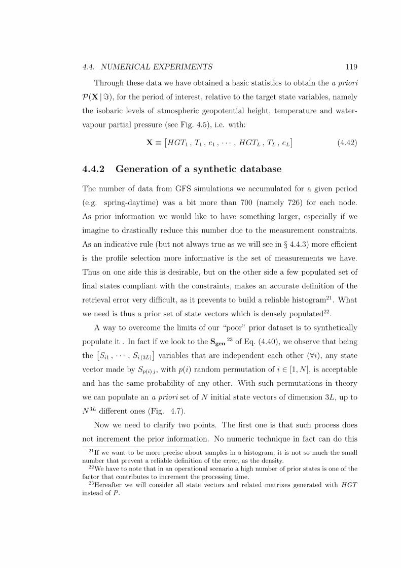
4.4. NUMERICAL EXPERIMENTS 119
Through these data we have obtained a basic statistics to obtain the a priori
P(X | =), for the period of interest, relative to the target state variables, namely
the isobaric levels of atmospheric geopotential height, temperature and water-
vapour partial pressure (see Fig. 4.5), i.e. with:
X ≡[HGT1 , T1 , e1 , · · · , HGTL , TL , eL
](4.42)
4.4.2 Generation of a synthetic database
The number of data from GFS simulations we accumulated for a given period
(e.g. spring-daytime) was a bit more than 700 (namely 726) for each node.
As prior information we would like to have something larger, especially if we
imagine to drastically reduce this number due to the measurement constraints.
As an indicative rule (but not always true as we will see in § 4.4.3) more efficient
is the profile selection more informative is the set of measurements we have.
Thus on one side this is desirable, but on the other side a few populated set of
final states compliant with the constraints, makes an accurate definition of the
retrieval error very difficult, as it prevents to build a reliable histogram21. What
we need is thus a prior set of state vectors which is densely populated22.
A way to overcome the limits of our “poor” prior dataset is to synthetically
populate it . In fact if we look to the Sgen23 of Eq. (4.40), we observe that being
the[Si1 , · · · , Si (3L)
]variables that are independent each other (∀i), any state
vector made by Sp(i) j, with p(i) random permutation of i ∈ [1, N ], is acceptable
and has the same probability of any other. With such permutations in theory
we can populate an a priori set of N initial state vectors of dimension 3L, up to
N3L different ones (Fig. 4.7).
Now we need to clarify two points. The first one is that such process does
not increment the prior information. No numeric technique in fact can do this
21If we want to be more precise about samples in a histogram, it is not so much the smallnumber that prevent a reliable definition of the error, as the density.
22We have to note that in an operational scenario a high number of prior states is one of thefactor that contributes to increment the processing time.
23Hereafter we will consider all state vectors and related matrixes generated with HGTinstead of P .
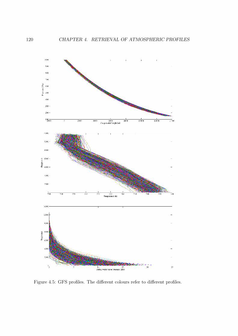
120 CHAPTER 4. RETRIEVAL OF ATMOSPHERIC PROFILES
Figure 4.5: GFS profiles. The different colours refer to different profiles.
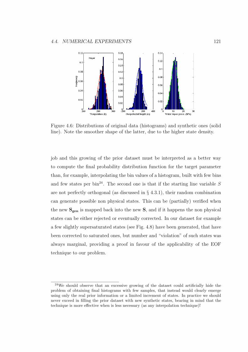
4.4. NUMERICAL EXPERIMENTS 121
Figure 4.6: Distributions of original data (histograms) and synthetic ones (solidline). Note the smoother shape of the latter, due to the higher state density.
job and this growing of the prior dataset must be interpreted as a better way
to compute the final probability distribution function for the target parameter
than, for example, interpolating the bin values of a histogram, built with few bins
and few states per bin24. The second one is that if the starting line variable S
are not perfectly orthogonal (as discussed in § 4.3.1), their random combination
can generate possible non physical states. This can be (partially) verified when
the new Sgen is mapped back into the new S, and if it happens the non physical
states can be either rejected or eventually corrected. In our dataset for example
a few slightly supersaturated states (see Fig. 4.8) have been generated, that have
been corrected to saturated ones, but number and “violation” of such states was
always marginal, providing a proof in favour of the applicability of the EOF
technique to our problem.
24We should observe that an excessive growing of the dataset could artificially hide theproblem of obtaining final histograms with few samples, that instead would clearly emergeusing only the real prior information or a limited increment of states. In practice we shouldnever exceed in filling the prior dataset with new synthetic states, bearing in mind that thetechnique is more effective when is less necessary (as any interpolation technique)!
122 CHAPTER 4. RETRIEVAL OF ATMOSPHERIC PROFILES
Figure 4.7: Distributions of synthetic data at different layers. Different coloursmark different pressure layers, namely the 1st, the 5th and the 15th for the targetparameters.
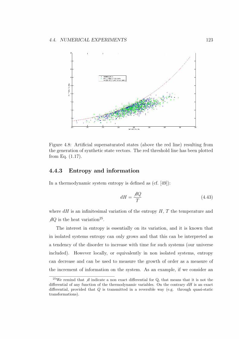
4.4. NUMERICAL EXPERIMENTS 123
Figure 4.8: Artificial supersaturated states (above the red line) resulting fromthe generation of synthetic state vectors. The red threshold line has been plottedfrom Eq. (1.17).
4.4.3 Entropy and information
In a thermodynamic system entropy is defined as (cf. [49]):
dH =6 dQT
(4.43)
where dH is an infinitesimal variation of the entropy H, T the temperature and
6 dQ is the heat variation25.
The interest in entropy is essentially on its variation, and it is known that
in isolated systems entropy can only grows and that this can be interpreted as
a tendency of the disorder to increase with time for such systems (our universe
included). However locally, or equivalently in non isolated systems, entropy
can decrease and can be used to measure the growth of order as a measure of
the increment of information on the system. As an example, if we consider an
25We remind that 6 d indicate a non exact differential for Q, that means that it is not thedifferential of any function of the thermodynamic variables. On the contrary dH is an exactdifferential, provided that Q is transmitted in a reversible way (e.g. through quasi-statictransformations).
124 CHAPTER 4. RETRIEVAL OF ATMOSPHERIC PROFILES
isothermal compression of an ideal gas of N molecules from the volume V0 to the
volume V1, the variation of entropy is:
∆H = −Nk lnV0
V1
(4.44)
being k the Boltzmann constant. Microscopically this isothermal decrease in the
volume corresponds to a decrease in the number Ω of possible modes that can
give the macroscopic state. In fact we can consider an arbitrarily small volume
∆V that contains a gas molecule, thus defining its position: so doing the number
of “possible positions”, that gives the number of the possible coordinate modes
for a molecule, is given by V/∆V . The decrease in the number of possible modes
corresponds to an increase in the information we have on the molecules, i.e. on
the microscopic state of the system. Then for a molecule we could express the
information I as:
I = k lnΩ0
Ω1
= k lnV0/∆V
V1/∆V= k ln
V0
V1
(4.45)
and for the whole gas of molecule we would have:
I = Nk lnΩ0
Ω1
(4.46)
that is, from Eq. (4.44), I = −∆H
We can easily see an analogy between possible microscopic modes and possible
state vectors in our problem, i.e. between the decrease of modes due to the
thermodynamic transformation, bringing to the new volume constraint, and the
selection of possible state vectors due to our measurement constraints (whose
application represents our transformation). Such analogy has not to be literally
assumed, as an increment of information is correctly assessed by changes in the
shape of the probability density functions and not simply by the reduction of
the number of compatible states. In fact, if we imagine a measurement that
rejects a number states in a random way, it must not bring any information:
accordingly the shape of the probability density function remains unchanged
while the number of states diminish26.26This difference between an ideal simple thermodynamic system and our problem can be
4.4. NUMERICAL EXPERIMENTS 125
With this in mind, we can then use the above variation of H to derive a
measure of the information. The Gibbs theorem asses that in a system the
whole entropy is the sum of partial entropies (e.g. of different gases). In this
way Gibbs managed to formulate an expression for entropy, which is (cf. [34]):
H = −k∑i
pi ln pi (4.47)
that is defined apart from additive constants (irrelevant in the estimation of
entropy variations).
In the theory of information Shannon demonstrated that there is only a pa-
rameter that univocally respects all the requirements of logic consistency for the
measurement of the information content for a distribution, and that parameter
has the same expression of H, apart from a multiplicative factor, that have not a
specific meaning as in thermodynamics, and that consequently can be arbitrarily
chosen, as well as the basis of the logarithm operator (cf. [36]) .
Entropy and its variation are consequently the basic features we have evalu-
ated to test the gain of information in our numerical experiments. Namely for
any measurement, we have evaluated the gain of information both through the
changes in the entropy defined as follows:
H = −∑i
pi log pi (4.48)
and through the relative entropy Hrel, defined as:
Hrel =∑i
pCi logpCipAi
(4.49)
Hrel compares the difference between two distribution, A and C. As an example
of application A could be the a priori probability density function and C the
resulting one after the application of the measurement constraints. We can see
(−∆H) as a measure of the change in width between two distributions, i.e.
approximately explained by the fact that our knowledge of the possible states (before and afterthe constraint application) is given by the a priori dataset which: even in the most optimisticcase, it is always much far than being “complete”, and as a consequence it can be used only toinfer probabilities and not to directly evaluate the number of possible states and its variation.
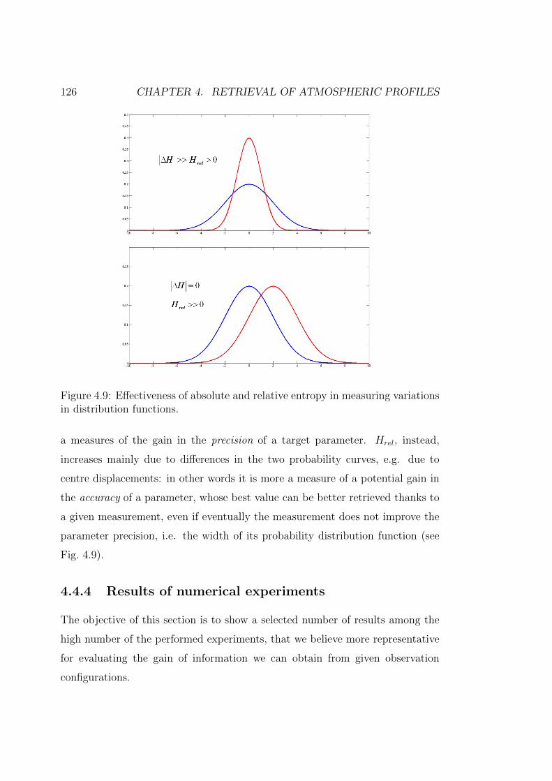
126 CHAPTER 4. RETRIEVAL OF ATMOSPHERIC PROFILES
Figure 4.9: Effectiveness of absolute and relative entropy in measuring variationsin distribution functions.
a measures of the gain in the precision of a target parameter. Hrel, instead,
increases mainly due to differences in the two probability curves, e.g. due to
centre displacements: in other words it is more a measure of a potential gain in
the accuracy of a parameter, whose best value can be better retrieved thanks to
a given measurement, even if eventually the measurement does not improve the
parameter precision, i.e. the width of its probability distribution function (see
Fig. 4.9).
4.4.4 Results of numerical experiments
The objective of this section is to show a selected number of results among the
high number of the performed experiments, that we believe more representative
for evaluating the gain of information we can obtain from given observation
configurations.
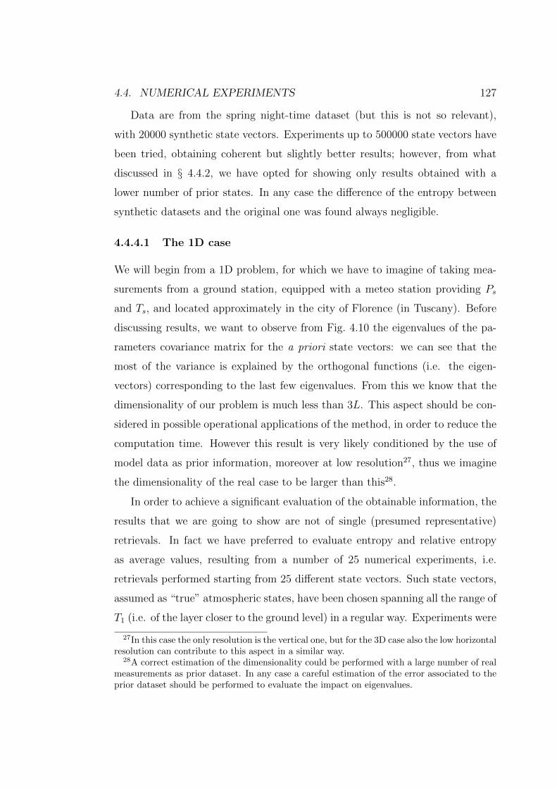
4.4. NUMERICAL EXPERIMENTS 127
Data are from the spring night-time dataset (but this is not so relevant),
with 20000 synthetic state vectors. Experiments up to 500000 state vectors have
been tried, obtaining coherent but slightly better results; however, from what
discussed in § 4.4.2, we have opted for showing only results obtained with a
lower number of prior states. In any case the difference of the entropy between
synthetic datasets and the original one was found always negligible.
4.4.4.1 The 1D case
We will begin from a 1D problem, for which we have to imagine of taking mea-
surements from a ground station, equipped with a meteo station providing Ps
and Ts, and located approximately in the city of Florence (in Tuscany). Before
discussing results, we want to observe from Fig. 4.10 the eigenvalues of the pa-
rameters covariance matrix for the a priori state vectors: we can see that the
most of the variance is explained by the orthogonal functions (i.e. the eigen-
vectors) corresponding to the last few eigenvalues. From this we know that the
dimensionality of our problem is much less than 3L. This aspect should be con-
sidered in possible operational applications of the method, in order to reduce the
computation time. However this result is very likely conditioned by the use of
model data as prior information, moreover at low resolution27, thus we imagine
the dimensionality of the real case to be larger than this28.
In order to achieve a significant evaluation of the obtainable information, the
results that we are going to show are not of single (presumed representative)
retrievals. In fact we have preferred to evaluate entropy and relative entropy
as average values, resulting from a number of 25 numerical experiments, i.e.
retrievals performed starting from 25 different state vectors. Such state vectors,
assumed as “true” atmospheric states, have been chosen spanning all the range of
T1 (i.e. of the layer closer to the ground level) in a regular way. Experiments were
27In this case the only resolution is the vertical one, but for the 3D case also the low horizontalresolution can contribute to this aspect in a similar way.
28A correct estimation of the dimensionality could be performed with a large number of realmeasurements as prior dataset. In any case a careful estimation of the error associated to theprior dataset should be performed to evaluate the impact on eigenvalues.

128 CHAPTER 4. RETRIEVAL OF ATMOSPHERIC PROFILES
Figure 4.10: Eigenvalues of the covariance matrix.
done retrieving profiles only from ground Ps and Ts measurements, then adding
a single measurement of tropospheric delay, DL. Errors (i.e. the tolerances) that
we have used in the retrieval we present are 5.0hpa, 2.0K and 1.0 cm for Ps,
Ts and DL respectively. Errors on Ps and Ts are not evaluated as instrumental
errors, that would be much lower, but as representativeness uncertainties. These
values in fact are point measurements of parameters that instead should refer
to a finite area, defined by our grid representation of the atmosphere. Even if
this is a 1D problem we are still working in a virtual cell, that in our case is
given by the horizontal resolution of the model, which has been the source of
our prior state distributions Errors have been thus estimated according to such
cell dimension. The error on DL have been then estimated on the basis of the
evaluations made in § 3, assuming to average a number of observations from the
same satellites for few minutes29.
In Fig. 4.11 we can observe the different decrease of entropy (i.e. the gain
of information) from the starting a priori distribution due to the ground mea-
surements and the addition of the GNSS delay, for all the target parameters at
29We remind that GPS standard ground stations provide delay measurements each second.The error we adopted is thus smaller than the error to be associated to a single observation,but at the same time larger than what could be obtained by averaging all possible observationsfor a relatively long time, that in some cases can be of few millimetres.
4.4. NUMERICAL EXPERIMENTS 129
different levels. The range of variation of the entropy is from the curve of the
prior distribution to 0. The prior distribution in fact is what the procedure re-
turns if no measurement is available or if measurement errors are larger than the
prior distribution itself. On the contrary H = 0 means that the distribution is a
Dirac δ, i.e. that is the most informative distribution30. We find that:
• ground data provide a lot of information that constrains also values at
higher levels, and this is not surprising once we have verified a large corre-
lation among layers (probably in our dataset larger than what is realistic);
• GNSS delays bring relevant additional information at all levels, with major
effects on water vapour e (as expected), but with a great contribution also
on of T and HGT , the latter especially at high levels where the entropy of
the prior distribution is larger31.
In addition, from the relative entropies of Fig. 4.12, reminding that information
increases for increasing Hrel, we find that:
• GNSS delays can bring a strong variation in distribution centres, changing
the retrieved best values. This happens at all levels, but particularly at the
lower levels of HGT and e, where the main components of the delay come
from, due to higher gas density and average water vapour concentrations.
From Eq. (4.49) we see that the relative entropy has a minimum value of 0, that
corresponds to no difference between the two compared distributions. Again this
is the case of the procedure returning the prior distribution (i.e. when H is
30Reminding that the limit of the ratio of two functions is equal to the ratio of their deriva-tives, such that:
limp→0+
p log p = limp→0+
log p1p
= limp→0+
−1p1p2
= limp→0+
−p = 0−
and referring to Eq. (4.48), if we have pi = 0 ∀i 6= j and pj = 1, we obtain H = 0. The Diracδ is the limit of the former case for infinitesimal bin width.
31We remind that reducing the distribution width of HGT defined with respect to fixedpressure levels, is essentially equivalent to improve the precision with which pressure is known,in a scheme where the height levels are fixed and pressure is a variable depending on height.
130 CHAPTER 4. RETRIEVAL OF ATMOSPHERIC PROFILES
maximum). In turn, we have a maximum value for the relative entropy when
the distribution after measurements has all states just in one bin, and this bin
corresponds to the one that was the least probable in the prior distribution32.
Such threshold values are reported in Fig. 4.12 too.
An example of retrieved profiles (i.e. of a state vector) is given in Fig. 4.13,
where we have assumed to have the ground measurements of pressure and tem-
perature and a measurement of the zenith GNSS delay. In the example in figure
the synthetic measurements have been corrupted with an artificial error, shifting
their values of half of the full tolerance range, with respect to the chosen “true”
observable ones. It results a good capability of the procedure to retrieve the tar-
get parameters, even at high levels. However to correctly quantify this aspect we
should have a more realistic prior dataset: once we had it, it would make sense
to try retrievals also with a larger number of observations (meteo and GNSS),
as we should realistically have in many situations.
4.4.4.2 The 3D case
Among the infinite number of numerical experiments we could imagine to test
the 3D retrieval process, we have decided to set up the most simple configuration
in order to have a restricted set of results but of clear meaning. In our theoretical
experimental set up, we assume to have a second ground station, equipped with
meteorological sensors, in the town of Siena (in Tuscany), about 50 km distant
from Florence33. We imagine also to have the Florence GNSS station switched-
off . Our target parameters are still the atmospheric profiles over Florence as in
§ 4.4.4.1, but here we want to evaluate the variation of information we have from
the prior distribution due to simply the ground meteorological measurements in
Florence (same as the 1D case), than adding the ground meteorological measure-
ments performed in Siena, and finally integrating the set of measurements with a
32We remind that to bins with 0 states have been assigned a minimum value of 1/N asexplained in § 4.3.1. If there are n0 void bins, the assigned minimum number is 1/(N n0 , andany of these bins can be chosen with no impact on the result.
33This distance is the minimum one we could adopt in this work, according to the resolutionof the source dataset.
4.4. NUMERICAL EXPERIMENTS 131
GNSS delay measured in Siena for different slant path angles, towards Florence
(i.e. in the vertical plane including Florence and Siena). This is the minimum
set up we can imagine to evaluate the information content that a slanting signal
path can bring to neighbouring cells, not owing other ground GNSS stations. We
must say that this is a very limiting configuration with respect to some real situ-
ations: we use in fact a single signal path very distant from the target point. On
the contrary there are now a lot of regions with several available and less distant
paths (e.g. the distribution of ground stations in the GPS network in Tuscany,).
From our results we can however infer the effect of more measurements on our
retrieval procedure, as through Eq. (4.34) we know that measurements impact
directly on the precision and accuracy of the retrieved target parameters, through
their value and precision (i.e. through their probability density function).
State vector components have been doubled to account for the variables over
Siena, and accordingly we have enlarged the prior dataset and related matrixes.
The diagonalisation has confirmed the high correlations of parameters also on
the horizontal scale34, part of which is again presumably due to model resolution
and approximations.
The main results are summarised in the graphs of Fig. 4.14 and Fig. 4.15. The
relevant horizontal correlation make the information contribution from Siena very
important also on Florence, both due to ground meteorological measurements
and due to GNSS observations. The difference in the observation inclinations
gives a less marked contribution, that is a bit more relevant for the precision of the
highest levels. However we have to bear in mind that even with the highest slant
angle considered, i.e. 75 (equivalent to 15 over the horizon) our hypothetical ray
path would pass over Florence at an height greater than 13 km (but this is what
we could do with our source dataset). In addition the high horizontal correlation
of the source data damps the possibility to differentiate the information from
measurements, that all results from interpolations of horizontal features. In
34With respect to the 1D case, with two points we have found that the same variance (e.g.the 99%) is explained by about one third more eigenvalues, against the double we should havefor horizontally uncorrelated variables.
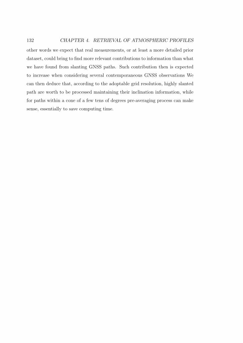
132 CHAPTER 4. RETRIEVAL OF ATMOSPHERIC PROFILES
other words we expect that real measurements, or at least a more detailed prior
dataset, could bring to find more relevant contributions to information than what
we have found from slanting GNSS paths. Such contribution then is expected
to increase when considering several contemporaneous GNSS observations We
can then deduce that, according to the adoptable grid resolution, highly slanted
path are worth to be processed maintaining their inclination information, while
for paths within a cone of a few tens of degrees pre-averaging process can make
sense, essentially to save computing time.
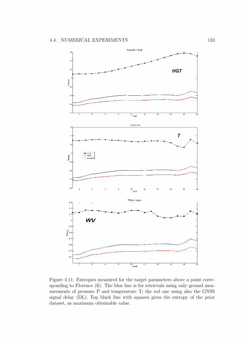
4.4. NUMERICAL EXPERIMENTS 133
Figure 4.11: Entropies measured for the target parameters above a point corre-sponding to Florence (fi). The blue line is for retrievals using only ground mea-surements of pressure P and temperature T; the red one using also the GNSSsignal delay (DL). Top black line with squares gives the entropy of the priordataset, as maximum obtainable value.
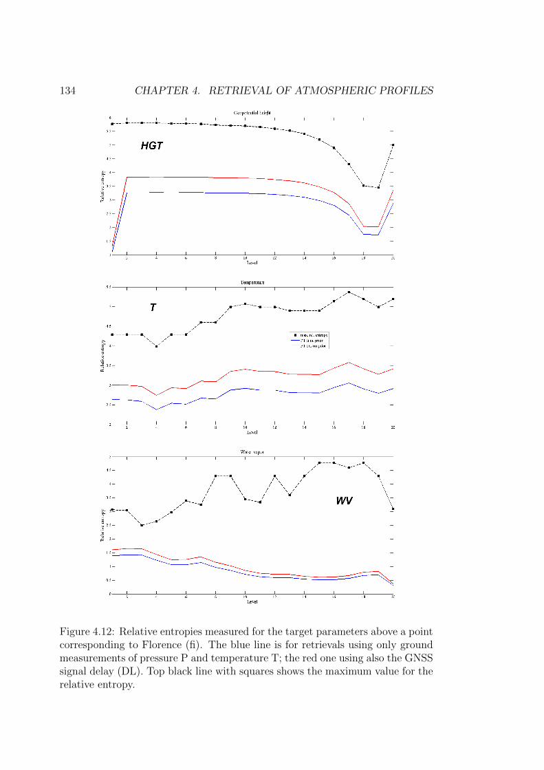
134 CHAPTER 4. RETRIEVAL OF ATMOSPHERIC PROFILES
Figure 4.12: Relative entropies measured for the target parameters above a pointcorresponding to Florence (fi). The blue line is for retrievals using only groundmeasurements of pressure P and temperature T; the red one using also the GNSSsignal delay (DL). Top black line with squares shows the maximum value for therelative entropy.
4.4. NUMERICAL EXPERIMENTS 135
Figure 4.13: Example of a state vector retrieval using ground measurements forpressure, temperature and GNSS signal delay. Red lines are “true” parameterprofiles; blue lines the retrieved ones. The yellow background is given by priorstates. 1σ error bar are shown too. The geopotential height HGT is given as afunction of the pressure P : a zoom is included to better show retrieval results.Temperature T and water vapour partial pressure e instead are given as functionof the height (through HGT ). Synthetic measurements are generated from thecorresponding observables corrupted with errors about half of the measurementuncertainties.
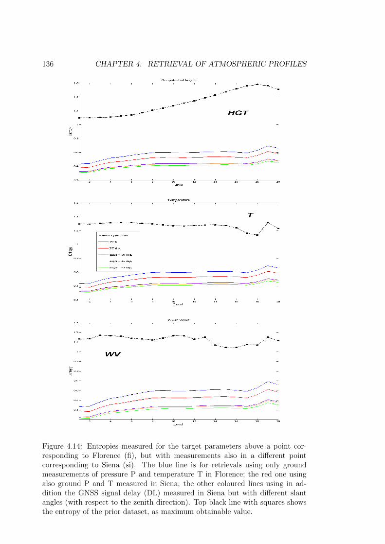
136 CHAPTER 4. RETRIEVAL OF ATMOSPHERIC PROFILES
Figure 4.14: Entropies measured for the target parameters above a point cor-responding to Florence (fi), but with measurements also in a different pointcorresponding to Siena (si). The blue line is for retrievals using only groundmeasurements of pressure P and temperature T in Florence; the red one usingalso ground P and T measured in Siena; the other coloured lines using in ad-dition the GNSS signal delay (DL) measured in Siena but with different slantangles (with respect to the zenith direction). Top black line with squares showsthe entropy of the prior dataset, as maximum obtainable value.
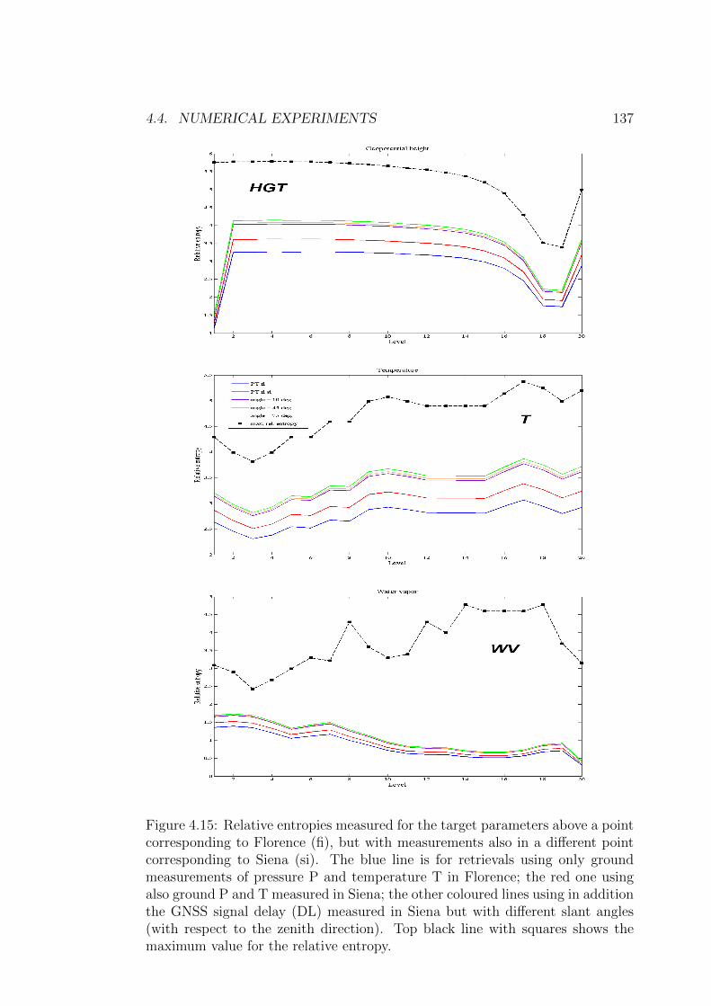
4.4. NUMERICAL EXPERIMENTS 137
Figure 4.15: Relative entropies measured for the target parameters above a pointcorresponding to Florence (fi), but with measurements also in a different pointcorresponding to Siena (si). The blue line is for retrievals using only groundmeasurements of pressure P and temperature T in Florence; the red one usingalso ground P and T measured in Siena; the other coloured lines using in additionthe GNSS signal delay (DL) measured in Siena but with different slant angles(with respect to the zenith direction). Top black line with squares shows themaximum value for the relative entropy.

138 CHAPTER 4. RETRIEVAL OF ATMOSPHERIC PROFILES
Chapter 5
Lines of future development
The are several future developments of the technique described in § 4 and they
are analysed in this short but dedicated chapter. Some of them endue not only
with a scientific interest opening the possibility for more precise retrieval of
atmospheric parameters (as in §§ 5.1, 5.2and 5.4), but also contribute towards an
optimisation of the process computing-time and of follow-up applications (§ 5.3),
or to extension to additional target parameters potentially of great interest (as
in § 5.5).
5.1 Improvement of the a priori dataset
In several part of § 4.4 we have stressed the problem of using a prior source
dataset made of a relatively small number of states and in addition non from real
measurements, but from simulations of a global Numerical Weather Prediction
(NWP) model. We have partially solved some of the problems that derive from
the poor number of prior states with a generation of synthetic data (as described
in § 4.4.2), but with the awareness that any synthetic densification of the prior
dataset cannot upgrade its information content. We have already motivated
why we believe that these limitations have not jeopardised the main conclusions
arising from the test results of § 4.4.4, but for moving from simple synthetic
experiments for testing the procedure to reliable assessments of the obtainable
precisions, and then to real measurements, we would definitely need a different
139
140 CHAPTER 5. LINES OF FUTURE DEVELOPMENT
a priori.
The ideal solution would be to have a large number of direct measurements,
(e.g. radiosondes), but this is not practicable as we want to fill a prior dataset
with several years of data, with some measurements per day (say each 3÷ 6hr)
for each grid node of our retrieval configuration. An alternative could be to use
of NWP model data from Limited Area Model (LAM) simulations, at list to
integrate available measurements. As an example, a not too demanding solution
for us to be implemented in the future, could be to use the operational simulations
run at LaMMA. These are 20 different simulations per day based on the Weather
Research and Forecasting (WRF) modelling system, 14 initialised with GFS
global model data, and 6 with ECMWF ones, with different resolutions, from 3
to 15 km of horizontal grid resolution, with 35 tropospheric levels.
5.2 Shape of the error probability functions
In § 4.3.1 we have derived a formal expression for the retrieval method we have
developed (i.e. Eq. (4.34)). We have also explained that for an easier imple-
mentation (and for saving computing time) we have adopted a square shape
for the measurement error distributions, defined by a given tolerance value (see
Eq. (4.35)), as the choice of a different error shape would not have changed
substantially the results.
However, apart from computational aspects, a different choice for the er-
ror distribution shape, for instance a truncated Gaussian, could be preferable,
because likely more realistic. Using such a distribution would have required
a modification of the retrieval implementation. Instead of selecting the states
whose related observables are compliant with the measurements within the tol-
erance ranges, using a “bell-shaped” error distribution function we should also
store the probability values associated to the distance between the observables
and the available measurements, and then use such information in the histogram
generation for the retrieved parameters.
There are two additional aspects in favour of adopting bell-shaped curves as
5.3. TRANSITION TO CONTINUOUS VARIABLES 141
error distributions.
The first aspect is that a bell-shaped distribution is non zero for a larger do-
main than a “quasi-equivalent” square one1. This means that the final number of
selected states will be higher, of course with compliant states non equally prob-
able. In other words with a more realistic error function we would “naturally”
have more dense final histograms, with equal prior states, avoiding the loss of
part of the information due to a coarse choice of the error distribution shape.
The second aspect is a bit more tricky. Let us assuming to have a number
of measurements of the same observables giving exactly identical results, i.e.
the same expected values. Errors distribution will be of course the same for all
measurements, according to the adopted error model. We could expect that a
sequence of identical results should enforce the confidence in the goodness of the
measured value, improving its precision or the precision of linked retrievals (i.e.
reducing the width of its error distribution or of the error distributions of related
retrievals). All bell-shaped distributions for errors confirm this expectation, both
for direct measurements and for indirect retrieval as ours, as can be seen from
Eq. (4.35). Square shaped errors are an exception, as they state the perfect
equivalence of measurements within a range: if results are not identical, then we
have a reduction of the error range (or a similar effect on any related retrieval),
but in case of identical measurements this cannot happen, and our procedure
formal expression or numeric implementation confirms this. As in our numerical
experiments we have not supposed to process more measurements of the same
observable, this has surely not affected our results, but generally this is a risk to
be avoided.
5.3 Transition to continuous variables
We have already said that EOF could be used to reduce the problem dimen-
sionality. An interesting approach, partially alternative, is the use of orthogonal
1This “quasi-equivalence” could be assessed by the same standard deviation.
142 CHAPTER 5. LINES OF FUTURE DEVELOPMENT
analytical functions. This would need to express the prior states through a given
set of these functions, trying to find an acceptable compromise between the error
committed in the transition from discrete samples to analytical functions, and
the dimension of the basis of functions used to do the job. A proper choice of the
basis is essential to be able to represent the large part of the variance through
few function elements. Fourier series could result a reasonable choice of an or-
thogonal basis suitable for representing horizontal patterns in a limited domain.
Instead for the vertical domain different bases could be necessary to better repro-
duce the different patterns of pressure, temperature and water vapour, according
to their physics.
Assuming to be able to address this issue, we could proceed with state vectors
made by a reduced number of functions coefficients, and the problem dimension-
ality could be a bit furthermore reduced with an EOF analysis.
The main advantages arising from such an approach would be that:
• we would manage to confine all necessary approximations (e.g. on prob-
lem dimensionality and required interpolations) at the initial stage of the
retrieval procedure;
• we would efficiently contain the computing time due to:
– a relevant reduction of the problem dimensionality,
– the potential to analytically solve at least some parts of the retrieval
problem;
• we would produce analytical solutions for the retrieved parameters (i.e.
continuous state vectors), with great benefits for possible following appli-
cations requiring different scales.
5.4 Upgrading to a 4D processing
The retrieval procedure we have developed has never taken into account the
opportunity to exploit the information from a time sequence of measurements.
5.5. GROWING THE STATE VECTORS FOR NEW MEASUREMENTS 143
We have always proceeded considering each measurement as unique, with the
only available prior information given by our a priori dataset. The reason of
this, is that we should primarily state the amount of information we could gain
from different basic measurement configuration, independently on the dynamic
of the events.
However one of the advantages of GNSS observations is that they are almost
continuous, and the refresh time of modern meteorological stations is also very
high. In real operational observations we should not waste the information con-
tent of previous measurements, that need to be propagated, through a more or
less simple evolution model for the target parameters, and than exploited into
new retrievals for additionally constraining the prior dataset2.
This is one of the aspects that could drastically improve the capability of
precise retrievals in our problem.
5.5 Growing the state vectors for new measure-
ments
One of the interesting properties of the procedure we have implemented is its
flexibility, meaning that it can work independently on number, type, precision
and geographical distribution of available measurements. Of course measurement
availability and characteristics affect retrieval accuracy, but not the capability
to produce a result, that at worst will be no more informative than the prior
probability distribution.
Another property is that, in principle, it is easily upgradeable to include addi-
tional target parameters, that can be added as new variables in the state vector,
becoming new retrievable parameters. Of course the real capability of retrieving
a given parameter depends on a number of factors, included the availability of
measurements that strongly depend on it. Difference in typical time as well as
spatial scales of variation are among the information that can be valuably used,
2This roughly summarises the basics of sound techniques based on Kalman filtering (e.g.cf. [34]).
144 CHAPTER 5. LINES OF FUTURE DEVELOPMENT
in order to decouple the contribution of different parameters, helping to retrieve
their value.
In a core part of a FP7 research proposal, submitted on a call for Galileo
scientific applications3, we have proposed to evaluate the capability of our ap-
proach to address the issue of measuring atmospheric target parameters over the
sea. The marine environment, including the atmospheric component, is definitely
under-sampled, while there is an increasing demand for information related also
to potential (commercial) applications. The idea is to test the feasibility of ex-
ploiting ships as slow-moving platforms, where “slow” identify platforms whose
displacement during the measurement time is much less than the typical spa-
tial scale of variation of the target parameters, and whose velocity fluctuations
(e.g. due to waves) occur on time scales much smaller than the measurement
one (that in turn will be smaller than the typical time scale of variation to be
resolved for the target parameter). Clearly, with respect to the problem of mea-
suring atmospheric delays from fixed stations, we have to manage an additional
(slow-changing) variable, the receiver position, which is not known a priori with
negligible uncertainty and thus become part of the additional parameters in the
sate vector. What is to be tested is if the large number of GNSS satellites with
similar characteristics, that offshore will be simultaneously in view with Galileo
operational in addition to GPS, could allow to effectively track at the same time
positions and atmospheric delays, with the necessary accuracy.
The flexibility of the proposed approach could find valuable applications also
in very different issues with respect to the one has been developed for. One for
all could be the water loading estimation problem. The interest in measuring
water masses is obvious and the water loading effect in crustal displacement is
3The mentioned proposal is COSMEMOS, that has been submitted to the Call: FP7-GALILEO-2011-GSA-1, Area: Scientific Application; Topic: Galileo and EGNOS for scientificapplications and innovative applications in new domains. It has been ranked and it is in thegroup of proposals selected for funding.
5.5. GROWING THE STATE VECTORS FOR NEW MEASUREMENTS 145
known, and it has already been subject of retrieval through GNSS signal based
techniques (e.g. cf. [44]). Variations to be measured are in this case of the order of
millimetres, thus comparable with a number of other effects analysed in § 3, that
should be carefully modelled and included in the retrieval process. Of course
spatial and time scales of interest are in this application completely different
from the one addressed in this work and a specific analysis should be performed
in order to understand to what extent a technique similar to the one developed
could extract useful information and return retrievals with the required precision.

146 CHAPTER 5. LINES OF FUTURE DEVELOPMENT
Concluding remarks
The core objective of this work is the evaluation of the potential capabilities of
navigation satellite signals to retrieve basic atmospheric parameters. The interest
on this subject arises on one side from the increasing demand of meteorological
information at more and more detailed spatial and temporal scales, and on the
other side from the increasing availability of GNSS measurements, both for the
expansion of the ground networks of fixed receivers (mainly settled for precise
positioning) and for the programmed launch of new GNSS platforms, in primis
the European Galileo system.
A number of “receipts” already exists regarding GNSS atmospheric appli-
cations, mainly oriented to evaluate zenith integrated water vapour quantities,
often expressed in terms of precipitable water. In the present work we have tried
an alternative approach to verify on which extent it is possible to retrieve pro-
files of parameters of interest from one single GNSS observation, integrated with
ancillary meteorological ground measurements, in the perspective of using the
“forest” of navigation signals that already exist and that is going to densify.
To this purpose we have performed a capillary study of the assumptions more
or less explicitly contained in the common processing steps of navigation signals.
We have started from the “very beginning”, including an analysis of the origin
of the atmospheric refractive index at the frequencies of interest (i.e. the GNSS
operating ones), in order to identify the dependency on the atmospheric features
and to quantify the approximations contained in the geometrical optics scheme,
adopted for modelling the navigation signal behaviour.
We have implemented a simulator to evaluate phase delay and bending of
147
148 CHAPTER 5. LINES OF FUTURE DEVELOPMENT
a GNSS signal travelling across a standard atmosphere. Then it has been up-
graded to manage general atmospheric scenarios, including the possibility of non
monotonic path curvature variations (useful for observations low on the horizon).
With reference to the present GPS satellite constellation, we have accurately
analysed the numerous processing steps necessary to obtain that part of the
signal containing only tropospheric effects, and the various errors components
associated to each step. Such analysis have been integrated by a study of a small
set of real data from the ground GPS network in Tuscany4.
With such acquired background information we have tried to overcome the
limits of standard approaches adopted in GNSS meteorological applications, with
the aim of measuring at first zenith profiles of all atmospheric features affecting
the refractive index (instead of mean water vapour values) and then to extend
the method to 3D retrievals. To this aim we have demonstrated the unsuitability
of the classical tomography for addressing the 3D problem, due to the varying
geometries of GNSS observations from irregularly distributed ground stations, in
favour of a flexible probabilistic approach.
A probabilistic procedure has been thus designed for measuring vertical dis-
cretised profiles of pressure, temperature and water vapour and their associated
errors at each vertical level. The data of input are of course GNSS tropospheric
delays and surface measurements of temperature and pressure. The procedure
has been upgraded to include simultaneous retrievals from more points, i.e. to
potentially perform 3D retrievals. It has been structured to process unevenly
distributed measurements and to be able to work independently on the number
and precision of observations that are from time to time available.
Numerical experiments on a synthetic dataset have been set up with the main
aim of quantifying the information that could be gained from such approach, us-
ing entropy and relative entropy as testing parameters. The results demonstrate
the potential of GNSS data in providing valuable information for 3D retrieval of
4Such network has been set up for supporting precise positioning and consists of heteroge-neous receivers that are not born to primarily support GPS meteorological applications.

5.5. GROWING THE STATE VECTORS FOR NEW MEASUREMENTS 149
temperature and water vapour.
However this cannot be considered a conclusive work for two main reasons.
The first one could be said “practical”, and it is related to the way we have
implemented the proposed procedure, which is too computing-time demanding
to allow an immediate application to real operational measurements. The second
one is more “theoretical” as it refers to the precision we could obtain for the target
parameters with, when applying our method to a real measurement situation.
The answer to this question can be only partially inferred in this work, as we
have not worked with a strongly reliable prior dataset, and (being aware of this)
we have not tried retrievals with a synthetic experimental set up similar to a real
one (i.e. with several GNSS observations and ground meteo stations).
These problem will be matter of future development, as they have been finally
pointed out, with specific indications on how to overcome some of the identified
limitations and to develop further improvements towards both scientific and op-
erational advancements. One of this line has been already judged of interest from
the refereeing panel of the European FP7 Galileo programme, as it is part of a
submitted project proposal, that has been positively ranked and whose activity
are going to start in the second half of year 2011.

150 CHAPTER 5. LINES OF FUTURE DEVELOPMENT
Bibliography
[1] Air Resources Laboratory (ARL) of NOAA’s Office of Oceanic and At-
mospheric Research (OAR), 2010. United States Department of Commerce
[http://ready.arl.noaa.gov/].
[2] Ashby N., 2003: Relativity in the Global Positioning System. Living Rev.
Relativity 6, Boulder [http://www.livingreviews.org/lrr-2003-1].
[3] Bao-Yen Tsui, J., 2000: Fundamental of global positioning system receivers:
a software approach. New York, 2000, John Wiley & Sons Inc., 240 pp.
[4] Bevis, M., S. Businger, T. A. Herring, C. Rocken, R. A. Anthes, and R. H.
Ware, 1992: GPS meteorology: remote sensing of atmospheric water vapor
using the global posisioning system. J. Geoph. Research, 97 (D14), 787-801.
[5] Bilitza, D., 2001: International Reference Ionosphere 2000. Radio Sci.,
36(2), 261-275.
[6] Brandt, S., 1978: Statistical and Computational Methods in Data Analysis.
North-Holland Publishing Company, Amsterdam, 418 pp.
[7] Brizard, A. J., 2004: Introduction to lagrangian and hamiltonian mechanics.
Department of Chemistry and Physics, Saint Michaels College, Colchester,
VT, 173 pp.
[8] Buck, A. L., 1981: New equations for computing vapor pressure and en-
hancement factor. J. Appl. Meteorol., 20, 1527-1532.
151
152 BIBLIOGRAPHY
[9] Chao, C. C., 1972: A model for tropospheric calibration from daily surface
and radiosonde ballon measurements. Tech. Memo. Calif. Inst. of Technol.
Jet Propulsion Lab., 391-350.
[10] Clough, S. A., Y. Beers, G. P. Klein, and L. S. Rothman, 1973: Dipole
moment of water of stark measurements of H2O. J. Chem. Phys., 59 (5),
2254-2259.
[11] Dach, R., U. Hugentobler, P. Fridez, and M. Meindl, 2007: Bernese GPS
Software Version 5.0. Astronomical Institute, University of Bern.
[12] Davidson, J. M., and D. W. Trask, 1985: Utilization of mobile VLBI for
geodetic measurements. IEEE Trans. Geosci. Remote Sens., GE-23, 426-437.
[13] Davis, J. L., T. A. Herring, I. I. Shapiro, A. E. Rogers, and G. Elgered, 1985:
Geodesy by radio interferometry: Effects of atmospheric modeling errors on
estimates of baseline length. Radio Sci., 20, 1593-1607.
[14] Debye, P., 1929: Polar Molecules. Chemical Catalog Company, New York,
172 pp.
[15] Doornbos, E., M. Foster, B. Fritsche, T. van Helleputte, J. van den Ijssel,
G. Koppenwallen, H. Lohr, D. Rees, P. Visser, and M. Kern, 2009: Air
density models Derived from multi-satellite drag observations. ESA’s Second
Swarm International Science Meeting, 24-26 June GFZ Potsdam, Germany
[http://www.congrex.nl/09c24/].
[16] Eckart, C., 1948: The approximate solution of one dimensional wave equa-
tions. Rev. Mod. Phys., 20, 399-417.
[17] Elgered, G., J. L. Davis, T. A. Herring, and I. I. Shapiro, 1991: Geodesy by
radio interferometry: Water vapor radiometry for estimation the wet delay.
J. Geophys. Res., 96, 6541-6555.
[18] Fermi, E., 1972: Termodinamica. Bollati Boringhieri Ed., Torino.
BIBLIOGRAPHY 153
[19] Feynman, R. P., R. B. Leighton, and M. Sands, 1963: The Feynman
Lectures on Physics. Addison-Wesley Publishing Company, Massachusetts,
Vol. 1, 515 pp.
[20] Grupta, A. K., T. F. Mri, and G. J. Szkely, 2000: How to transform Corre-
lated Randon Variables into Uncorrelated Ones. Appl. Mathematics Letters,
13, 31-33.
[21] ICD, 1993: Interface Control Document - Navstar GPS Space Segment /
Navigation User Interfaces (ICD-GPS-200, 1993).
[22] Jackson, J. D., 1962: Classical electrodynamics. John Wiley & Sons Inc.,
New York, 641 pp.
[23] Khinchin, A. I., 1978: Fondamenti matematici della teoria
dell’informazione. Cremonese Ed., Roma, 129 pp.
[24] Kline, P. A., 1997: Atomic Clock Augmentation For Receivers Us-
ing the Global Positioning System. PhD Thesis, Ohio University -
Avionics Engineering Center [http://scholar.lib.vt.edu/theses/available/etd-
112516142975720/].
[25] Klobuchar, J.A., 1987: Ionospheric time-delay algorithm for single-
frequency GPS Users. IEEE Transactions, AES-23(3), 325-331.
[26] Lomb, N. R., 1976: Least-squares frequency analysis of unequally spaced
data. Astrophysics and Space Science, 39, 447-462.
[27] Lower, S. K., 1998: Thermal physics (and some chemistry) of the atmo-
sphere. J. Chem. Educ., 75 (7), 837-840.
[28] Lowry, A. R., C. Rocken, S. V. Sokolovskiy, and K. D. Anderson, 2002:
Vertical profiling of atmospheric refractivity from ground based GPS. Radio
Sci., 37 (3), 13.1-13.10, doi:10.1029/2000RS002565.
154 BIBLIOGRAPHY
[29] Misra, P., and P. Endge, 2001: Global Positioning System-Signal, Measure-
ments, and Performance. Ganga-Jamuna Press, Lincoln, Masssachusetts, 390
pp.
[30] Owens, J. C., 1967: Optical refractive index of air: Dependence on pressure,
temperature and composition. Appl. Opt., 6, 51-58.
[31] Parkinson, B. W., and J. J. Jr. Spilker, 1996: Global Positioning System:
Theory and Applications, Vols.1 and 2. American Institute of Aeronautics,
370 LEnfant Promenade, SW, Washington, DC.
[32] Pearson, K., 1901: On Lines and Planes of Closest Fit to Systems of Points
in Space. Philosophical Magazine, 2 (6), 559-572.
[33] Prasad, R., and M. Ruggieri, 2005: Applied Satellite Navigation Using GPS,
GALILEO, and Augmentation Systems. Artech House Mobile Comunication
Series, Boston, 290 pp.
[34] Rodgers, C., 2000: Inverse Methods for Atmospheric Sounding: Theory
and Practice. World Scientific Publishing, Series on Atmospheric, Oceanic
and Planetary Physics, Vol. 2.
[35] Saastamoinen, J., 1972: Atmospheric correction for the troposphere and
stratosphere in radio ranging of satellites. in The Use of Artificial Satellites
for Geodesy, Geophys. Monogr. Ser., vol. 15, edited by S. W. Henriksen, et
al., 247-251.
[36] Shannon, C. E., 1948: A Mathematical Theory of Communication The Bell
System Technical Journal, Vol. 27, 379423.
[37] Shannon, C. E., 1949: Communication in the presence of noise. Proc. Insti-
tute of Radio Engineers, 37 (1), 10-21.
[38] Stull, R. B., 2000: Meteorology for Scientists and Enginieers. Brooks/Cole
Thomson Learning, U.S.A, 502 pp.
[39] Thayer, D., 1974: An improved equation for the radio refractive index of
air. Radio Sci., 9, 803-807.
[40] Toraldo di Francia, G., and P. Bruscaglioni, 1988: Onde elettromagnetiche.
Zanichelli Ed., 705 pp.
[41] Tralli, D. M., and S. M. Lichten, 1990: Stochastic estimation of tropospheric
path delays in global positioning system geodetic measurements. Bull. Geod.,
64, 127-159.
[42] Ulaby, T. F., K. R. Morore, and K. A. Fung, 1943: Microwave remote
sensing, active and passive. Library of Congress Cataloging in Publication
Data, Artech-Hause, Londra, Vol.I, 456 pp.
[43] U.S. Standard Atmosphere, 1976. U.S. Government Printing Office, Wash-
ington, D.C.
[44] Van Dam, T., Wahr, J., Milly, P. C. D., Shmakin, A. B., Blewitt, G.,
Lavallee, D. and Larson, K. M., 2001: Crustal displacements due to conti-
nental water loading Geophys. Res. Lett., 28, 651-654.
[45] Van Vleck, J. H., and V. F. Weisskopf, 1945: On the shape of collision-
broadened lines. Rev. Mod. Phys., 17, 227-236.
[46] Vultaggio, M., 2009: Lezioni di navigazione satellitare. Universita di Napoli
Partenophe - Facolta di Scienze e Tecnologie, Napoli.
[47] Wallace, J., and P. V. Hobbs, 1977: Atmospheric science an introductory
survey. Academic Press, 467 pp.
[48] Xu Guochang, 2007: GPS Theory, Algorithms and Applications. 2nd edi-
tion, Berlin Heidelberg 2007, Springer-Verlag, 340 pp.
[49] Zemansky, M. W., 1987: Calore e Termodinamica. Zanichelli Ed., Bologna,
Vol. I, 255 pp.
155

156
Acknowledgements
My first thanks goes to Prof. Rolando Rizzi for his continuous support along
the non easy steps of this work, for the fruitful discussions we had together and
for his constant transfer of experience, enthusiasm and motivation.
I have in part drawn on the knowledge of my colleagues Andrea Antonini and
Riccardo Benedetti. With them I had so many recurrent and intensive arguments
to the point that in many aspects we cannot, at present, almost distinguish whom
the contributed ideas belong to.
Samantha Melani, Andrea Orlandi and especially Luca Rovai are gratefully
acknowledged for their technical support in the development of some aspects of
this work; Prof. Kai Borre for his careful advices in the comprehension of some
GPS signal criticalities.
I wish to acknowledge in a particular way also Carlo Brandini, Simone Cristo-
fori, Bernardo Gozzini and Chiara Lapucci for their encouragement and for hav-
ing volunteered to be my back-up in solving daily work issues.
A special thanks goes to my children, Davide and Sofia, who have been un-
derstanding and who managed to cope with my absence during the period these
pages were written.
Finally, I am grateful to my wife Lucia. For her, there are no words to
describe the meaning she has in every single event of my life.
GFS data for this study are from NOAA’s National Operational Model Archive
and Distribution System (NOMADS).
157

158