probabilistic ml part 1
TRANSCRIPT

1
P. Agius – Spring 2008
Probabilistic ML modelsPart 1
Recommended text:Pattern Recognition and Machine LearningBy Christopher Bishophttp://research.microsoft.com/~cmbishop/PRML/
These slides: mostly Ch 1&2Other relevant Chs: 8 (available online), 9
P. Agius – Spring 2008
Contents• Part 1
– Introduction to probability theory– Baye’s theorem– Likelihood functions in curve fitting– Probability distributions
• Part 2– Graphical models– Mixture Models
• Part 3– An example of some of my current work using
probabilistic models for biological data

2
Introduction to Probability
• Experiments, Outcomes, Events and Sample Spaces
• What is probability?
• Basic Rules of Probability
• Probabilities of Compound Events
MT2004
Olivier GIMENEZ
Telephone: 01334 461827
E-mail: [email protected]
Website: http://www.creem.st-and.ac.uk/olivier/OGimenez.html

3
1. Probability
Probability is a branch of mathematics
Deals with quantifying and modelling the uncertainty relating to random experiments
But what's a random experiment?
Any process with a number of possible outcomes, but the occurence of any outcome is not known in advance
Think of tossing a coin (head/tail) or rolling a die (1,...,6) e.g.
1.1 Definitions
The sample space ΩΩΩΩ is the set of all possible outcomes
A sample point ωωωω is a possible outcome i.e. a point in Ω
An event, e.g. A, is a set of possible outcomes satisfying a given condition (so A is a set of sample points)
The null event Ø contains no sample point -impossible event

4
1.1 Definitions
Example 1: Toss a coin
Ω = head,tail=H,T
Let A be event 'a head is obtained', then A = H
Example 1': Toss 2 coins
Ω = TT,TH,HT,HH
Let B be event 'at least one H is obtained', then B = TH,HT,HH
1.1 Definitions
Example 2: Roll a die and note the number shown
Ω = 1,2,3,4,5,6
Let A be event 'the number shown is even', then A = 2,4,6
Let B be event 'the number shown is ≤ 4', then B = 1,2,3,4
When studying a random experiment, it's important to spend time to define both the sample space and the events

5
1.1 Definitions
Let A and B be any two events in sample space Ω, then:
A ∪∪∪∪ B = union of A and B = the set of all outcomes in A or B (i.e. only A, only B in both A and B)
Example 2 (cont'd): Roll a die
A event 'the number shown is even', i.e. A = 2,4,6B event 'the number shown is ≤ 4', i.e. B = 1,2,3,4
A ∪ B = 2,4,6 ∪ 1,2,3,4 = 1,2,3,4,6
1.1 Definitions
Let A and B be any two events in sample space Ω, then:
A ∩∩∩∩ B = intersection of A and B = the set of all outcomes in A and B --- joint probabilityand denoted as P(A,B) and verbalized as ‘probability of A and B’.
Example 2 (cont'd): Roll a die
A event 'the number shown is even', i.e. A = 2,4,6B event 'the number shown is ≤ 4', i.e. B = 1,2,3,4
A ∩ B = 2,4,6 ∩ 1,2,3,4 = 2,4

6
1.1 Definitions
Let A be any event in sample space Ω, then:
AC = the set of points that do not occur in A, but do occur in Ω
Ω
AAc
Wenn diagram
1.1 Definitions
Let A be any event in sample space Ω, then:
AC = the set of points that do not occur in A, but do occur in Ω
Example 2 (cont'd): Roll a die
A event 'the number shown is even', i.e. A = 2,4,6
AC = 1,3,5 = event 'number shown is odd'

7
1.1 Definitions
Let A and B be any two events in sample space Ω, then:
A and B are mutually exclusive or disjoint if A ∩∩∩∩ B = Ø
Ω
AB
1.2 Axioms of Probability
Let Ω be a sample space. A probability Pr is a function which assigns a real number Pr(A) to each event A such that:
1) 0 ≤ Pr(A) ≤ 1 for any event A ⊆ Ω
2) Pr(Ω) = 1 (honesty condition)
3) If A1,...,An are a finite sequence of disjoint events,
Pr(A1 ∪ A2 ... ∪ An) = ∑Pr(Ai)
i.e. the probability that either of the events Ai happens is the sum of the probabilities that each happens
8
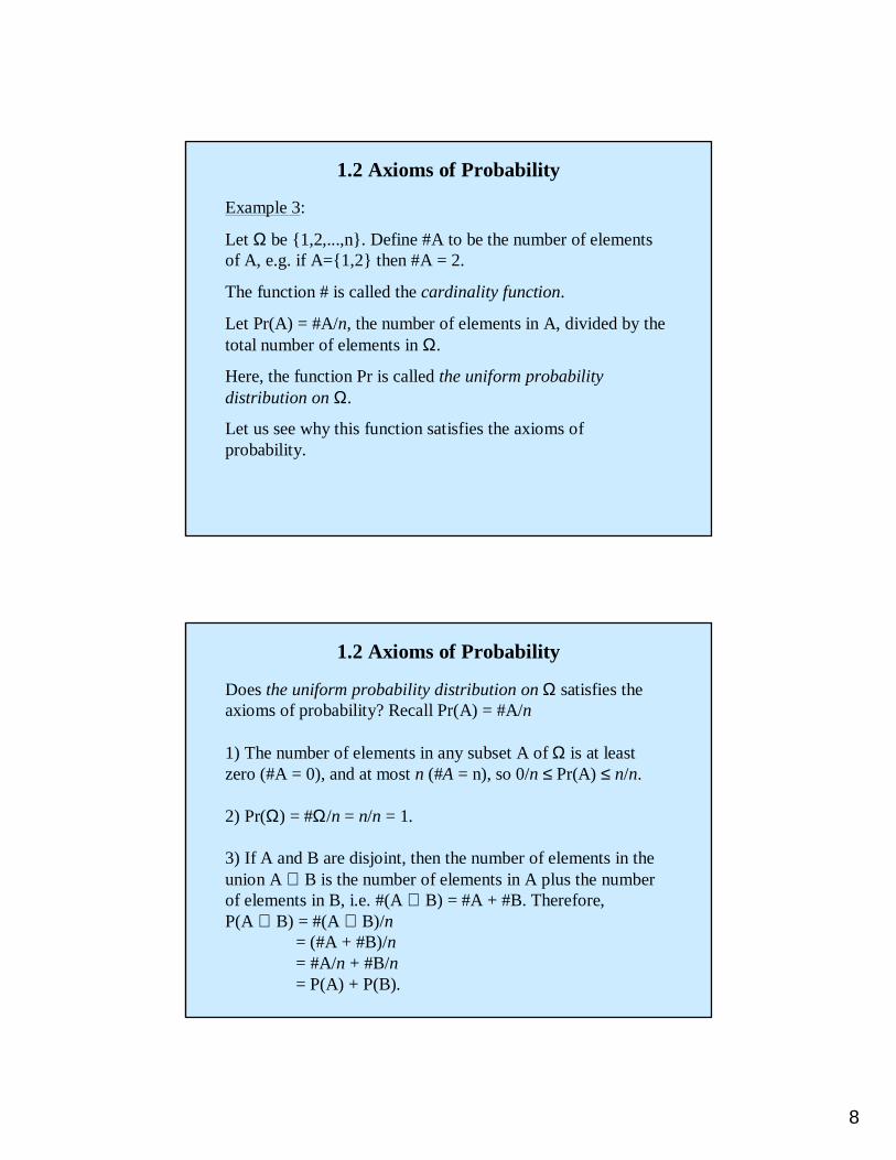
1.2 Axioms of Probability
Example 3:
Let Ω be 1,2,...,n. Define #A to be the number of elements of A, e.g. if A=1,2 then #A = 2.
The function # is called the cardinality function.
Let Pr(A) = #A/n, the number of elements in A, divided by the total number of elements in Ω.
Here, the function Pr is called the uniform probability distribution on Ω.
Let us see why this function satisfies the axioms of probability.
1.2 Axioms of Probability
Does the uniform probability distribution on Ω satisfies the axioms of probability? Recall Pr(A) = #A/n
1) The number of elements in any subset A of Ω is at least zero (#A = 0), and at most n (#A = n), so 0/n ≤ Pr(A) ≤ n/n.
2) Pr(Ω) = #Ω/n = n/n = 1.
3) If A and B are disjoint, then the number of elements in the union A ∪ B is the number of elements in A plus the number of elements in B, i.e. #(A ∪ B) = #A + #B. Therefore, P(A ∪ B) = #(A ∪ B)/n
= (#A + #B)/n= #A/n + #B/n= P(A) + P(B).

9
1.3 Conditional Probability
Let A and B be any two events in sample space Ω, such that Pr(B) > 0 (i.e. Pr(B) ≠ 0).
Then the conditional probability of A, given that event B has already occured is denoted by Pr(A|B) and is defined by:
1.3 Conditional Probability
Example 4:
Suppose that we randomly choose a family from the set of all families with 2 children. Then, Ω = (g,g),(g,b),(b,g),(b,b) (b=boy, g=girl) where we assume that each event is equally likely.
Given the family has a boy, what is the probability both children are boys?
10
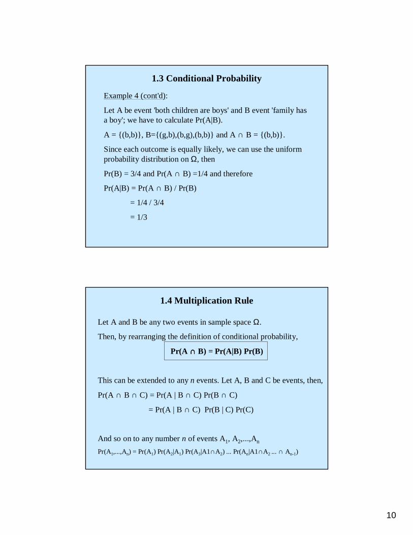
1.3 Conditional Probability
Example 4 (cont'd):
Let A be event 'both children are boys' and B event 'family has a boy'; we have to calculate Pr(A|B).
A = (b,b), B=(g,b),(b,g),(b,b) and A ∩ B = (b,b).
Since each outcome is equally likely, we can use the uniform probability distribution on Ω, then
Pr(B) = 3/4 and Pr(A∩ B) =1/4 and therefore
Pr(A|B) = Pr(A∩ B) / Pr(B)
= 1/4 / 3/4
= 1/3
1.4 Multiplication Rule
Let A and B be any two events in sample space Ω.
Then, by rearranging the definition of conditional probability,
Pr(A ∩∩∩∩ B) = Pr(A|B) Pr(B)
This can be extended to any n events. Let A, B and C be events, then,
Pr(A ∩ B ∩ C) = Pr(A | B ∩ C) Pr(B∩ C)
= Pr(A | B ∩ C) Pr(B | C) Pr(C)
And so on to any number n of events A1, A2,...,An
Pr(A1,...,An) = Pr(A1) Pr(A2|A1) Pr(A3|A1∩A2) ... Pr(An|A1∩A2 ... ∩ An-1)

11
1.5 Law of Total Probability
A set of disjoint (or mutually exclusive) events A1, A2,..., An on sample space Ω such that Ω = ∪ An, are said to be a partition of Ω.
Given a partition A1, A2,..., An on sample space Ω, the Law of Total Probability states that:
Pr(B) = ∑∑∑∑ Pr(B | Ai) Pr(A i)
1.6 Bayes Theorem
Let A1, A2,..., An be a partition of Ω with Pr(Ai) > 0 for i = 1,...n.
Let B be an event, such that Pr(B) > 0.
Then, the Bayes theorem states that:
Established by British cleric Thomas Bayes in his 1764 posthumously published masterwork, "An Essay Toward Solving a Problem in the Doctrine of Chances". See module MT4531.
Using the Law of Total Probability...

12
1.6 Bayes Theorem
Example 5: Drivers in the age-range 18-21 can be classified into 4 categories for car insurance purposes:
What is the probability that a randomly chosen driver came from category 3, given that he had no accident in the year?
0.20.40.60.8Pr(no accidents in a year)
15254020% of population in this category
4321Category
1.6 Bayes Theorem
Example 5 (cont'd): What is the probability that a randomly chosen driver came from category 3, given that he had no accidents in the year?
Let A be the event 'a person has no accidents' and Bi the event 'a person is from category i for i = 1,2,3,4'. We want to calculate Pr(B3|A)
Using Bayes Theorem, we have:
Recall the data:
So, from the data, we know that Pr(B3) = 0.25 and Pr(A|B3) = 0.4
0.20.40.60.8Pr(no accidents in a year)
15254020% of population in this category
4321Category

13
1.6 Bayes Theorem
Example 5 (cont'd): What is the probability that a randomly chosen driver came from category 3, given that he had no accidents in the year?
Using the Law of Total Probability, we have:
Pr(A) = ∑ Pr(A | Bi) Pr(Bi)
= 0.8 x 0.2 + 0.6 x 0.4 + 0.4 x 0.25 + 0.2 x 0.15
= 0.53
So, substituting into the general equation, we get:
1.7 Independence
Let A and B be any two events in sample space Ω.
Then, A and B are said to be independent if,
Pr(A ∩∩∩∩ B) = Pr(A) Pr(B)
This implies that
Pr(A|B) = Pr(A∩ B) / Pr(B)
Pr(A|B) = Pr(A)
That is, knowing whether or not B occurs gives no information about the occurrence of A.
Example of disjoint events: tossing a coinExample of dependent events: extracting cards from a deck of cards

14
1.7 Independence
Note: If events A and B are disjoint, this does NOT imply that A and B are independent.
Suppose that we toss a coin. Let A event 'obtain a head' and B 'obtain a tail', then A and B are disjoint (you can't have H and T at the same time).
Now, we have Pr(A) = Pr(B) = 1/2.
However the probability that a head is obtained, given that we have obtained a tail with the coin toss is 0, i.e. Pr(A|B) = 0...
Thus, we have A and B disjoint but A and B are not independent since Pr(A|B) ≠ Pr(A)
P. Agius – Spring 2008
ExpectationsThe expectation of f(x) over a discrete distribution is
For continuous variables, the probability density is
The conditional expectation with respect to a conditional distribution is
where E[f|y] denotes the expectation of f(x) given y.
E[f ] =∑
x
p(x)f(x)
E[f ] =
∫p(x)f(x)dx
Ex[f |y] =∑
x
p(x|y)f(x)

15
P. Agius – Spring 2008
Variance and Covariance
The variance of a variable x is
var(x) = E[x²] – E[x] ²
For two random variables x and y, the covariance is
cov[x,y] = Exy[xy] – E[x]E[y]
Covariance expresses the extent to which the two variables x and y vary together.
Question: What happens if x and y are independent?Think of coin tossing …
P. Agius – Spring 2008
Curve fitting
Given: inputs X = [x1, x2, . . . xN ] and outputs t = [t1, t2 . . . tN ].
Assumption: Given x, the corresponding value of t has a Gaussiandistribution with a mean of y(x, w).
So, p(t|x,w, β) = N(t|y(x,w), β−1) where β−1 is the precision, the variance.
Use training data (x, t) and maximum likelihood estimate to find w and β.

16
P. Agius – Spring 2008
Likelihood function
µ σ ²
Easier to maximize the log likelihood …
ln p(t|x,w, β) =
n∑
i=1
ln1
√2β−1
exp−1
2β−1(t− y(xi, w))
2
= −β
2
n∑
i=1
(t− y(xi, w))2 +
n
2(lnβ − ln 2π)
Maximizing the log likelihood is equivalent to minimizing the sum-of-squares error function.
The likelihood function is
p(t|x,w, β) =n∏
i=1
N (ti|y(xi, w), β−1)
P. Agius – Spring 2008
A more Bayesian approach
Introduce prior distributions over w like so:
p(w|α) = N(w|0, α−1I) = (α
2π)(M+1)/2 exp−
α
2wTw
Hyperparameter … controls the distribution of the model parameter ww is an M+1 vector for a
polynomial of order M+1
Using Baye’s theorem, the posterior distribution of w is proportional to the product of the prior distributionand the likelihood function
p(w|x, t, α, β) ∝ p(t|x, w, β)p(w|α)

17
P. Agius – Spring 2008
The predictive distribution resulting from a Bayesian treatment of polynomial curve fitting using an M=0 polynomial, with the fixedparameters alpha=0.0005 and beta=11.1 (corresponding to the known noise variance), in which the red curve denotes the mean of the predictive distribution and the red region corresponds to +-1 standard deviation around the mean.
P. Agius – Spring 2008
Classwork/Homework 4
From Bishop’s book (Q6 and Q10 and Q11)
6. Show that the covariance of two independent variables x and y is zero.
10. Suppose that two variables x and y are statistically independent.Show that the mean and variance of their sum satisfies
E[x+y]=E[x]+E[y]var[x+y]=var[x]+var[y]
11. By setting the derivatives of
ln p(x|µ, σ2) = ln
n∏
i
N (xi|µ, σ2)
with respect to µ and σ2 equal to zero,find the maximum likelihood estimate for µ and σ2.
Beta(µ|a, b) = Γ(a+b)Γ(a)Γ(b)µ
a−1(1− µ)b−1

18
P. Agius – Spring 2008
Classwork/Homework 4
From Bishop’s book – Ch1 Q 17 … for you math geeks only!!
17. The gamma function is defined by
Using integration by parts, prove the relation Г(x+1)=x Г(x). Show also that Г(1)=1 and hence that Г(x+1)=x! when x is an integer
Γ(x) =
∫ ∞
0
µx−1e−udu
P. Agius – Spring 2008
Probability Distributions (ch 2)
• Binary variables– Bernoulli, Binomial, Beta distributions
• Multinomial variables– The Dirichlet distribution
• The Gaussian distribution
• Non parametric methods, frequentist approaches
19
P. Agius – Spring 2008
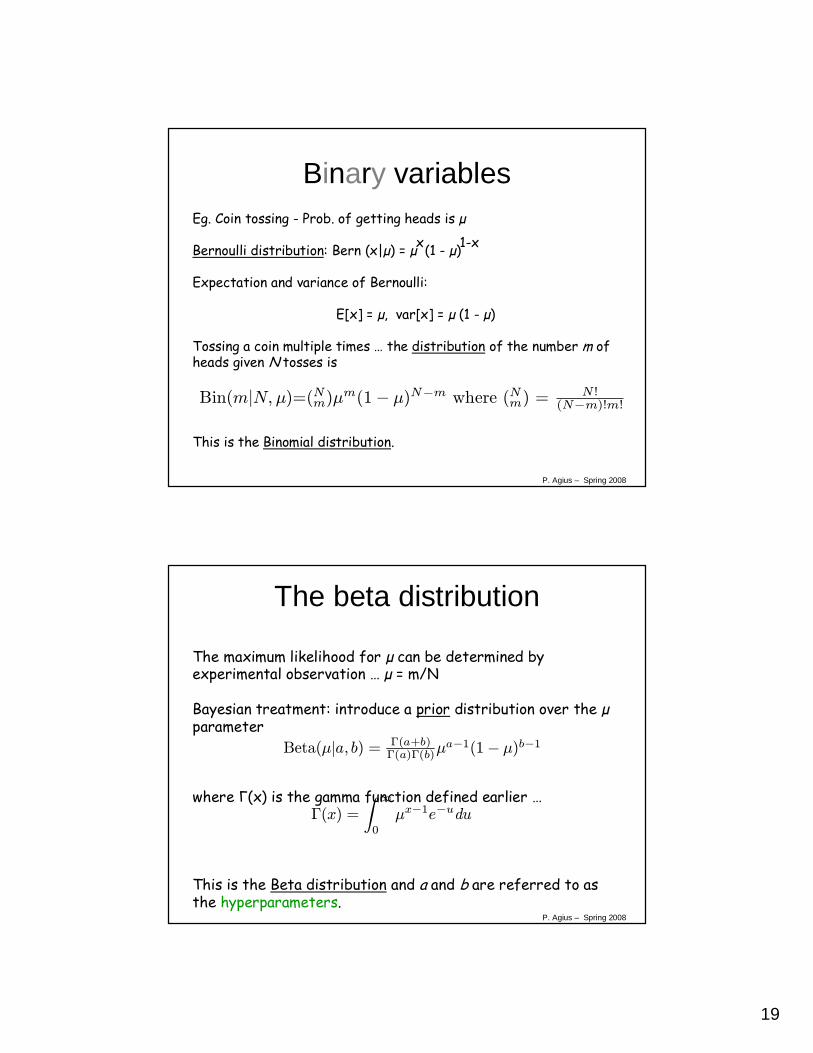
Binary variablesEg. Coin tossing - Prob. of getting heads is µ
Bernoulli distribution: Bern (x|µ) = µ (1 - µ)
Expectation and variance of Bernoulli:
E[x] = µ, var[x] = µ (1 - µ)
Tossing a coin multiple times … the distribution of the number m of heads given N tosses is
This is the Binomial distribution.
x 1-x
Bin(m|N, µ)=(Nm)µm(1− µ)N−m where (Nm) =
N!(N−m)!m!
P. Agius – Spring 2008
The beta distribution
The maximum likelihood for µ can be determined by experimental observation … µ = m/N
Bayesian treatment: introduce a prior distribution over the µ parameter
where Г(x) is the gamma function defined earlier …
This is the Beta distribution and a and b are referred to as the hyperparameters.
Beta(µ|a, b) = Γ(a+b)Γ(a)Γ(b)µ
a−1(1− µ)b−1
Γ(x) =
∫ ∞
0
µx−1e−udu

20
P. Agius – Spring 2008
Multinomial variablesNow consider variables that can take one of K possible values.Denote the probability of getting the kth state for an experiment by µk.
The distribution of x is given by
Consider a series of N experiments. What is the outcome now? (Earlier in binary situation, we had [0,1,0,0,1,1,…] … what now?)
The likelihood function for a dataset D of N experiments is
where mk is a count of the number of kth states.
p(x|µ) =K∏
k=1
µxkk
p(D|µ) =K∏
k=1
µmk
k
P. Agius – Spring 2008
The Dirichlet distributionLet’s use priors again!!! Now introduce a family of prior distributions for the parameters µk as follows:
where
The normalized form of this is the Dirichlet distribution:
0 ≤ µk ≤ 1,∑k µk = 1
α = [α1, . . . αk]
Dir(µ|α) =Γ(α0)
Γ(α1) . . .Γ(αK)
K∏
k=1
µαk−1k
p(µ|α) ∝
K∏
k=1
µαk−1k
α0 =K∑
k=1
αk

21
The Gaussian Probability Distribution Function
p(x) =1
σ 2πe
− (x −µ )2
2σ2gaussian
Plot of Gaussian pdf
x
p(x)
The Gaussian probability distribution is perhaps the most used distribution in all of science.Sometimes it is called the “bell shaped curve” or normal distribution.
Unlike the binomial and Poisson distribution, the Gaussian is a continuous distribution:
µ = mean of distribution (also at the same place as mode and median)σ2 = variance of distributiony is a continuous variable (-∞ ≤ y ≤ ∞)
Probability (P) of y being in the range [a, b] is given by an integral:
The integral for arbitrary a and b cannot be evaluated analytically.The value of the integral has to be looked up in a table
2
2
2
)(
21
)( σµ
πσ
−−=
y
eyp
dyedyypbyaPb
a
yb
a∫=∫=<<
−−2
2
2
)(
21
)()( σµ
πσ
Karl Friedrich Gauss 1777-1855
The total area under the curve is normalized to one by the σ√(2π) factor.
We often talk about a measurement being a certain number of standard deviations (σ) awayfrom the mean (µ) of the Gaussian.
We can associate a probability for a measurement to be |µ - nσ|from the mean just by calculating the area outside of this region.
nσ Prob. of exceeding µ±nσ0.67 0.51 0.322 0.053 0.0034 0.00006
It is very unlikely (< 0.3%) that a measurement taken at random from a Gaussian pdf will be more than ± 3σ from the true mean of the distribution.
P(−∞ < y < ∞) = 1σ 2π
e−(y−µ)2
2σ 2
−∞
∞∫ dy =1
-4 -3 -2 -1 1 2 3 4
0.1
0.2
0.3
0.48Shaded area gives prob . < 2σ <
-4 -3 -2 -1 1 2 3 4
0.1
0.2
0.3
0.48Shaded area gives prob . > 2σ <
95% of area within 2σ Only 5% of area outside 2σ
Gaussian with µ=0 and σ=1

22
For a binomial distribution:mean number of heads = µ = Np = 5000 standard deviation σ = [Np(1 - p)]1/2 = 50The probability to be within µ±1σ for this binomial distribution is:
For a Gaussian distribution:
Both distributions give about the same probability!
P = 104!
(104 −m)!m!m=5000−50
5000+50∑ 0.5m0.5104−m = 0.69
P(µ −σ < y < µ +σ ) = 1σ 2π
e−(y−µ)2
2σ 2
µ−σ
µ+σ∫ dy ≈ 0.68
Relationship between Gaussian and Binomial distribution The Gaussian distribution can be derived from the binomial (or Poisson) assuming:
p is finite N is very large we have a continuous variable rather than a discrete variable
An example illustrating the small difference between the two distributions under the above conditions: Consider tossing a coin 10,000 times.
p(head) = 0.5N = 10,000
Why is the Gaussian pdf so applicable? ⇒⇒⇒⇒ Central Limit Theorem A crude statement of the Central Limit Theorem:Things that are the result of the addition of lots of small effects tend to become Gaussian.A more exact statement:
Let Y1, Y2,...Yn be an infinite sequence of independent random variableseach with the same probability distribution.Suppose that the mean (µ) and variance (σ2) of this distribution are both finite.For any numbers a and b:
The C.L.T. tells us that under a wide range of circumstances the probability distribution that describes the sumof random variables tends towards a Gaussian distribution as the number of terms in the sum →∞.
limn→∞
P a < Y1+Y2 + ...Yn − nµσ n
< b
= 12π
e−1
2y 2
a
b∫ dy
Actually, the Y’s canbe from different pdf’s!
How close to ∞ does n have to be??
Alternatively we can write the CLT in a different form:
limn→∞
P a < Y − µσ / n
< b
= limn→∞
P a < Y − µσ m
< b
= 1
2πe
−12y2
a
b∫ dy

23
P. Agius – Spring 2008
Nonparametric methods
So far the probability distributions were governed by a small number of parameters that can be induced from the data.This is known as the parametric approach to density modeling
What about nonparametric approaches?Requires assumptions about the form of distribution
- histogram methodBuild a histogram of the data to get a density estimation
- kernel functionsUse a kernel function to obtain density estimates using hypercubes
- nearest neighbor methodsUseful for local density estimation
P. Agius – Spring 2008
More Classwork/Homework 4
From Bishop’s book, Ch 2
2.1 Verify that the Bernoulli distribution Bern (x|µ) = µ (1 - µ) satisfies the following properties:
E[x] = µ, var[x] = µ (1 - µ),
Some hypothesis-test questions using the Gaussian distribution.
1∑
x=0
p(x|µ) = 1
Defective Products: A large mail-order company has placed an order for 5,000 electric can openers with a supplier on the condition that no more than 2% of the devices will be defective. To check the shipment, the company tests a random sample of 400(n=400)of the can openers and finds that 11 (sample proportion=11/400=.0275) are defective. Does this provide sufficient evidence to indicate that the proportion of defective can openers in the shipment exceeds 2%? Test using α = .05 (significance level).

24
P. Agius – Spring 2008
Contaminated Soil Environmental Science & Technology (Oct. 1993)reported on a study of contaminate soil in The Netherlands. Seventy-two(n=72) 400-gram soil specimens were sampled, dried, and analyzed for the contaminant cyanide. The cyanide concentration [in milligrams per kilogram (mg/kg) of soil] of each soil specimen was determined using an infrared microscopic method. The sample resulted in a mean cyanide level of x-bar = 84mg/kg and a standard deviation of s = 80 mg/kg.Test the hypothesis that the true mean cyanide level in soil in The Netherlands exceeds 100 mg/kg. Use α = .10.Would you reach the same conclusion as in part a using α = .05? Using α =.01?