1 ml-pda and ml-pmht: comparing multistatic sonar...

1

ML-PDA and ML-PMHT: Comparing

Multistatic Sonar Trackers for VLO Targets

Using a New Multitarget Implementation

Steven Schoenecker, Peter Willett, Fellow, IEEE, and Yaakov Bar-Shalom,

Fellow, IEEE

Abstract

The Maximum Likelihood Probabilistic Data Association (ML-PDA) tracker and the Maximum

Likelihood Probabilistic Multi-Hypothesis (ML-PMHT) tracker are applied to five synthetic benchmark

multistatic active sonar scenarios featuring multiple targets, multiple sources and multiple receivers.

For each of the scenarios, Monte Carlo testing is performed to quantify the performance differences

between the two algorithms. Both methods end up performing well in situations where there is a

single target or widely-spaced targets. However, ML-PMHT has an inherent advantage over ML-PDA

in that its likelihood ratio has a simple multitarget formulation, which allows it to be implemeted as a

true multitarget tracker. This formulation, presented here for the first time, gives ML-PMHT superior

performance for instances where multiple targets are closely spaced with similar motion dynamics.

Keywords: ML-PDA, ML-PMHT, multitarget ML-PMHT, maximum likelihood, multistatic,

bistatic, sonar, tracking, expectation maximization, EM, multitarget, low observable.

I. INTRODUCTION

The Maximum Likelihood Probabilistic Data Association (ML-PDA) tracker and the Maximum

Likelihood Probabilistic Multi-Hypothesis (ML-PMHT) tracker are both simple, straightforward

algorithms that can be used in an active multistatic sonar framework. With some basic assump-

tions about a target (or targets) as well as the environment, likelihood ratios can be developed for

Original manuscript received 02/29/12. Revised manuscript received 8/31/12. Supported by ONR grants N00014-10-10412,

N00014-10-1-0029, and ARO grant W911NF-06-1-0467.

2

both algorithms and then optimized. The main difference between the two algorithms is in the

measurement-to-target assignment model; ML-PDA assumes that at most one measurement per

scan can originate from a target, while ML-PMHT allows for any number of measurements to

have originated from a target. While this assumption may reduce the appeal of the ML-PMHT

to some, the resulting algorithm does offer advantages in both its implementation (especially

fine-scale optimization) and in terms of its multitarget formulation.

The main contributions of this work are as follows: first, we theoretically develop and im-

plement ML-PMHT as a true multitarget tracker. As part of this, we find an expression for the

Cramer Rao Lower Bound (CRLB) for ML-PMHT and show that ML-PMHT seems to be a

statistically efficient estimator. As a result, this CRLB can be used as a covariance estimate for

ML-PMHT. Moving on to Monte Carlo testing, we provide an example of the capability of the

algorithms as very low observable trackers. (In this work we use “low observable” to refer to

targets with an SNR of 6-12 dB and “very low observable” to refer to targets with an SNR

of less than 6 dB.) We then demonstrate that while ML-PMHT and ML-PDA have identical

performance in single target cases, ML-PMHT is better than ML-PDA in multitarget cases or

when more than one measurement per scan is produced by the target.

The paper has the following structure: Section II briefly reviews the ML-PDA and ML-PMHT

(single target) log-likelihood ratios (a much more extensive discussion of this can be found in

[1] and [2]). Section III develops the novel multitarget ML-PMHT (including the CRLB for ML-

PMHT). Next, Section IV describes in detail the simulator used to create data for Monte Carlo

runs on the multistatic sonar scenarios considered; the five different scenarios used in this work

are presented here as well. Finally, Section V presents the results of the Monte Carlo testing.

We note that portions of this paper have appeared in [1] and [2]; this paper is an expansion

of these works. These previous works provided preliminary comparisons between ML-PDA and

ML-PMHT when they were both implemented in a sequential single target mode.

II. SINGLE TARGET ML-PDA VS. ML-PMHT

This section briefly describes the theory of the ML-PDA and the ML-PMHT (single target)

log-likelihood ratios (LLRs). It then shows how, under certain conditions, the ML-PDA LLR

and the ML-PMHT LLR should converge to the same expression. If such conditions are met,

there should be no performance difference between the two algorithms.

3

A. Likelihood Ratios

The ML-PDA concept was initially developed in [3]. Subsequently, in [4], [5], and [6] it was

applied in a multistatic active application, which is how we currently employ it. The assumptions

used to develop the ML-PDA likelihood ratio are [7], [8]:

• A single target is present in each frame with known detection probability Pd. Detections

are independent across frames.

• There are zero or one measurements per frame from the target.

• The kinematics of the target are deterministic. The motion is usually parameterized as a

straight line, although any other parameterizations (e.g. ballistic motion) can be used.

• False detections (clutter) are uniformly distributed in the search volume and their number

is Poisson distributed with known density.

• Amplitudes of target and false detections are Rayleigh distributed. The parameter of each

Rayleigh distribution is known (although the SNR may be tracked [9] in the case that it is

not known; then Pd becomes time-varying, which is easy to accomodate).

• Target measurements are corrupted with zero-mean Gaussian noise with known variance.

• Measurements at different times, conditioned on the parameterized state, are independent.

The assumptions for ML-PMHT are almost all the same as these, with one significant difference.

Instead of allowing only zero or one measurement per scan to originate from the target, the ML-

PMHT target-assignment model relaxes this constraint and allows any number of measurements

to originate from the target. The development of the ML-PDA and ML-PMHT likelihood ratios

has been presented in detail in [2]; we just summarize the results here.

The ML-PDA log-likelihood ratio (LLR) for a batch of data is

Λ(x, Z) =Nw∑i=1

ln

{1− Pd +

Pd

λ

mi∑j=1

p[zj(i)|x]ρj(i)}

(1)

In this equation, Pd is the target probability of detection in a scan, λ is the spatial clutter density,

Nw is the number of scans, and mi is the number of measurements in the ith scan. Next, zj(i)

is the jth measurement in the ith scan, p[zj(i)|x] is a target-centered Gaussian, and ρj(i) is the

amplitude likelihood ratio. Finally, x is the target state, and Z is the (entire) set of measurements

in the batch.

4

The ML-PMHT LLR is given by

Λ′(x, Z) =Nw∑i=1

mi∑j=1

ln

{π0 + π1V p[zj(i)|x]ρj(i)

}(2)

where π0 is the prior probability that a measurement is from clutter, π1 is the prior probability

that a measurement is from the target, and V is the search volume in the measurement space.

Note that the ML-PDA likelihood ratio (LR) is a product of a large sum (based on the total

probability theorem with respect to all the joint association events) while the ML-PMHT LR is

a double product of the sum of two terms (based on the total probability theorem for each

measurement separately, since each could be target- or clutter-originated, and these events

are assumed independent across measurements). This difference is the key in (i) allowing the

computation of the ML-PMHT CRLB in a much easier manner than for the ML-PDA CRLB

and (ii) allowing the extension of the ML-PMHT for multiple targets.

B. Relationship between ML-PDA and ML-PMHT

At first glance, the log-likelihood ratios for ML-PDA and ML-PMHT appear very dissimilar.

However, the terms in the log-likelihood ratio for ML-PDA are actually just a subset of the terms

in the likelihood ratio for ML-PMHT. Consider the ML-PMHT likelihood (not log-likelihood)

ratio for a single scan. This is written as

p1[Z(i)|x]p0[Z(i)|x] =

mi∏j=1

{π0 + π1V p[zj(i)|x]ρj(i)

}(3)

For any arbitrary number of measurements mi, this equation multiplied out yields

p1[Z(i)|x]p0[Z(i)|x] = πmi

0 +πmi−10 π1V

mi∑j=1

Nj+πmi−20 π2

1V2

mi−1∑j1=1

mi∑j2>j1

Nj1Nj2+ · · ·+πmi1 V mi

mi∏j=1

Nj (4)

where the terms Nj represent p[zj(i)|x], the target-centered Gaussian terms. It should also be

noted that the amplitude distribution ratios have been left out of the above equation — including

them would not affect the following discussion. Equation (4) is the ML-PMHT likelihood ratio

multiplied out for a single scan. It allows for more than one measurement to be assigned to a

target — the terms with products of target-centered Gaussians account for this case. In the case

of ML-PDA, the target assignment model allows only zero or one measurement to be assigned

to the target. The first term in (4) accounts for the case of zero measurements being assigned to

the target, and the second term in the equation accounts for the case of one measurement being

5

assigned to the target. The other terms account for two or more measurements being assigned

to the target. If the ML-PDA measurement model holds (or is at least very close to holding),

then the product of the probabilities of two (or more) measurements being from a target is

essentially zero and the terms with a product of two or more target-centered Gaussians in the

above expression go to zero. As a result, just the first and second terms are left. In this case,

we can claim the following relationships. First

1− Pd = πmi0 (5)

Then,

Pd = miπmi−10 π1 (6)

and, since E[mi] = λV , one can take (approximately),

πmi−10 π1V =

Pd

λ(7)

If these relationships hold, then the ML-PDA likelihood ratio and the ML-PMHT likelihood

ratio are equivalent.

III. MULTITARGET ML-PMHT

This section develops the multitarget formulation of ML-PMHT. It first discusses how it is

necessary to implement ML-PDA for multiple targets in somewhat of an ad-hoc manner. Next,

it presents the natural, multitarget version of the ML-PMHT LLR along with an elegant method

of optimizing it. Then it develops a covariance estimate of the ML-PMHT state vector via the

CRLB. Finally, it describes how to integrate these two concepts into a true multitarget tracking

framework for ML-PMHT.

A. ML-PDA Multitarget LLR

It is difficult to extend ML-PDA to multiple targets [10]. While it is technically possible to

write the multitarget ML-PDA log-likelihood ratio, to take into account all the joint association

events the number of terms increases rapidly with the number of targets, and the expression

becomes practically intractable for any more than just a few targets. As a result, in order to

handle multiple targets, the ML-PDA tracking framework treats scenarios with more than one

target as a sequence of single-target problems. For a batch of data, it optimizes the single-target

6

LLR (1), and if this value exceeds a certain threshold, a target is declared. (This threshold is

determined by fitting the local maxima formed by the clutter to an extreme value distribution

[11].) Next, the measurement that has the highest association probability with that solution is

excised from each scan, and the sequence is repeated for the next target. This method is not

elegant, but it has been shown to work reasonably well for multitarget scenarios in [12] and

[13].

B. ML-PMHT Multitarget LLR

In contrast to ML-PDA, the ML-PMHT LLR is very easily extended to a multitarget frame-

work. For K targets with state vectors x1, . . . ,xK , the multitarget LLR is expressed as

Λ′(x, Z) =Nw∑i=1

mi∑j=1

ln

(π0 + V

K∑k=1

πkp[zj(i)|xk]ρjk(i)

)(8)

where πk is the probability that a given measurement is from the k th target and∑K

k=0 πk = 1.

A benefit to using the ML-PMHT LLR formulation is that it is possible to optimize it with

a closed-form expression using expectation-maximization (EM) [14]. The process of optimizing

the ML-PMHT LLR for the single-target case was shown in [1]; here, we extend the optimization

to the multitarget case. The multitarget version of the cost function is

J(x, Z) =

K∑k=1

Nw∑i=1

mi∑j=1

{[zj(i)−Hkx]

TR−1ij [zj(i)−Hkx] + ln(|2πRij|)

}wjk(i) (9)

To briefly review, in the single target case, the ML-PMHT LLR can be optimized with EM as

long as there exists a linear relationship between the predicted measurement z and the state x,

where

x = [x0 x y0 y]T (10)

and the measurement matrix is

H =

[1 t 0 0

0 0 1 t

](11)

(For this to work, the measurements must obviously be in Cartesian space. While multistatic

measurements and covariances are typically in bearing/time-delay space, they can be converted

to Cartesian space following the work of [15] and [16].)

7

In the multitarget case for ML-PMHT, the state vector x becomes a 4K × 1 vector. (It is the

vector in (10) stacked K times.) The association probability wjk(i) is

wjk(i) =πkp[zj(i)|xk]ρjk(i)

π0/V +∑K

l=1 πlp[zj(i)|xl]ρjl(i)(12)

The matrix Hk in equation (9) is

Hk =

· · · 0 · · ·· · · 0 · · ·· · · 0 · · ·· · · 0 · · ·︸︷︷︸4(k − 1) columns

H

· · · 0 · · ·· · · 0 · · ·· · · 0 · · ·· · · 0 · · ·︸︷︷︸4(K − k) columns

(13)

This matrix is for the kth target — the (inner) H is that given by (11) . There are 4(k − 1)

vectors of zeros to the left of H and 4(K − k) vectors of zeros to the right of H. With these

definitions, the solution to the problem is a simple vector quadratic minimization, and is expressed

as

x =[ K∑

k=1

Nw∑i=1

mi∑j=1

wjk(i)HTkR

−1ij Hk

]−1K∑k=1

Nw∑i=1

mi∑j=1

wjk(i)HTkR

−1ij zj(i) (14)

C. ML-PMHT Cramer-Rao Lower Bound

Here, the Cramer-Rao Lower Bound (CRLB) for ML-PMHT is developed, and it is shown that

the ML-PMHT estimator is statistically efficient — i.e. the errors on the tracker state estimates

meet the CRLB. Additionally, it turns out that the CRLB for ML-PMHT can be computed real-

time; previous work on ML-PDA [8] showed that the CRLB for ML-PDA must be computed

off-line with Monte-Carlo integration. Put together, these factors lead to a valuable result, namely,

the CRLB calculation can be easily incorporated into the ML-PMHT tracking framework in order

to represent the tracker error.

The full derivation for the ML-PMHT Fisher Information Matrix (FIM) and CRLB is presented

in Appendix A; we summarize the key points in order to show why it is possible to compute

the CRLB real-time for ML-PMHT (again, as opposed to ML-PDA). First, consider a window

of ML-PMHT data with Nw scans. Since all measurements from scan to scan are assumed to

be independent, the FIM J of the total window can just be written as the sum of the individual

scans,

J =

Nw∑i=1

Ji (15)

8

After some, work (again, presented in Appendix A), a key point arises. The expression for Ji

is given as

Ji =

mi∑j=1

∫V

DTφ

[π1pτ1(aj)]2

|2πRj | e−(zj−φ)TR−1j (zj−φ)R−1

j (zj − φ)(zj − φ)TR−1j

p(zj|x)2 Dφ

mi∏l=1

p(zl|x)dZda(16)

Here, φ is the state-to-measurement conversion, and Dφ is the Jacobian of φ. Next, Rj is the

measurement covariance for the jth measurement in the scan. (Since (16) only deals with a single

scan, the i-subscripts are dropped.) Finally, dZ =∏mi

l=1 dzl and da =∏mi

l=1 dal. All p(zl|x) terms

for l �= j are separable and integrate to one, and the term for l = j is cancelled by one of the

terms in the denominator. All that is left within the integral is the single measurement z j . This

reduces the calculation to a dimension equal to the number of dimensions in the measurement,

plus one for the amplitude. This makes it possible for ML-PMHT to compute the FIM (and

thus the CRLB) real-time as part of the tracking framework. In contrast, for the ML-PDA FIM

calculation, a summation over all mi measurements in the scan remains in the denominator [8].

Thus, the dimensionality of the calculation in this case is approximately m i times the number

of measurement dimensions. As a result, the ML-PDA FIM must be calculated off-line with

Monte-Carlo integration.

After some work, the final expression for the ML-PMHT FIM is

Ji = DTφ

mi∑j=1

GTj

∫V

[π1pτ1(aj )]2

|2πRj | e−ξTj ξjξjξTj

π0pτ0(aj )

V+

π1pτ1(aj )√|2πRj |

e−12ξTj ξj

dξjdajGj

|Gj |Dφ (17)

where ξj is a dummy variable of integration with dimensionality equal to the measurement

dimensionality, and Gj is the Cholesky decomposition Rj . This is inserted into (15), and then

the CRLB is just taken as the inverse of the FIM.

At this point, the efficiency of the ML-PMHT estimator was checked by using this FIM to

calculate the normalized estimation error squared (NEES), which is given by

NEES = (x− xtruth)T J (x− xtruth) (18)

Scenario 1 (described in the sequel) was run 500 times, and for each run, the median NEES

value for a valid track was saved (there were multiple NEES values for a run due to the sliding

batch nature of the tracker implementation). The average of these NEES values came out to 4.15

with a 95 percent confidence interval of [3.97, 4.34]. The expected NEES for a 4-parameter state

9

−6 −4 −2 0 2 4 6−3

−2.5

−2

−1.5

−1

−0.5

0

0.5

Final Position

Initial Position

Figure 1. CRLB 95 percent uncertainty regions for initial and final positions.

vector is 4, which falls within the confidence interval. From this, the conclusion is that ML-

PMHT is a statistically efficient estimator. A subset of 20 of these runs is shown in Figure 1

with the 95 percent position uncertainty ellipses at the beginning and end of the runs plotted.

As expected, almost all of the solution points fall within their respective ellipses. The CRLB for

ML-PMHT (as opposed to ML-PDA) can be computed real-time and then be used to accurately

represent the error on the state estimate from the tracker.

D. ML-PMHT Multitarget Implementation

The ML-PMHT multitarget tracking framework was implemented in the track update sequence

by testing all existing tracks for “closeness.” Any tracks that were determined to be close were

grouped together and optimized with the multitarget ML-PMHT log-likelihood ratio formuation

in (8). Grouping tracks involved estimating the state covariance of all existing tracks. We let

the CRLB developed above represent the state covariance Cn for the nth target, and with this, a

χ2 test statistic [17] is evaluated for closeness between all possible pairs of active tracks in the

form

Smn = ∆xTmn(Cm +Cn)

−1∆xmn (19)

10

where ∆xmn = xm − xn (the difference of the state vector estimates between the mth and nth

track). All track pairs with a statistic Smn less than a given threshold are grouped together. More

than two tracks could belong to a group by the use of this association — to join a group, an

ungrouped track only had to meet the test described in (19) with one of the tracks already in

the group.

IV. SIMULATOR AND SIMULATIONS

This section describes in detail the simulator that was used to create the data for the Monte

Carlo runs and then presents the five scenarios used to compare ML-PDA and ML-PMHT.

A. Simulator Description

The Monte Carlo runs were performed using a multistatic simulator developed at the University

of Connecticut [18]. The simulator takes as input the source and receiver positions (all were

stationary in this work), as well as the number of targets and target geometries — this information

is all shown in Figures 5 through 14. Each transmitter generates a ping every 60 seconds, and for

each source-receiver pair (i.e., a scan), the simulator calculates the number, position, amplitude,

and Doppler of the clutter points, and the existence, position, amplitude, and Doppler of the

target returns. (All pings in the simulation were treated as being Doppler-sensitive.)

1) Clutter Measurement Generation: First, to generate the clutter points, the simulator cal-

culates the number of resolution cells that should be present. The number of resolution cells is

treated as a function of σaz and σt, the azimuthal and time-delay errors simulated for the system.

The number of azimuthal resolution cells is approximated as

Naz =360

BW(20)

where BW is the beamwidth of a receive beam in degrees. The simulator does not actually

form any beams; to get a value of BW , it makes the assumption that the clutter is distributed

uniformly in a beam, which gives σaz = BW/√12. This in turn leads to a final expression for

the number of azimuthal resolution cells,

Naz =

⌊360√12σaz

⌋(21)

(Here, “� �” signifies round towards the next lower integer.) For all of the scenarios in this

work, the azimuthal uncertainty was σaz = 5◦ (this and all other simulated error values are

11

provided together in Table II). Using similar logic, the number of delay (range) resolution cells

is calculated with the expression

Ndelay =

⌊tipt/2− tbt√

12σt

⌋(22)

Here, tipt is inter-ping time — 60 seconds throughout this work, and tbt is blanking time. This

value is determined by the amount of time sound takes to travel from source to receiver. Finally,

the number of resolution cells is simply given by the product of Naz and Ndelay.

With the number of resolution cells determined, the clutter is generated. For each scan, to

simulate the amplitudes of the clutter distribution, a number of random variables equal to the

number of resolution cells is generated. For the first five scenarios, the amplitude of this clutter

distribution was given a K-distribution. The probability distribution for the intensity of the clutter

(i.e. the amplitude squared) is given by [19], [20]

f(p) =2

λΓ(αk)

(p

λk

)(αk−1)/2

Kαk−1

(2

√p

λk

)(23)

where p > 0. Here, αk is a K-distribution parameter (αk = 0.5 throughout this work), λk = 1/αk,

and Kν is the Basset function (a modified Bessel function of the second kind) [21]. Random

variables from the distribution shown in (23) are generated via [20]

K = −Γλk lnU (24)

where U is a realization of a uniform random variable over the interval [0,1], and Γ is a realization

of a Gamma random variable with shape parameter α = αk and a scale parameter β = 1.

For clarity, we note that the simulator generates “amplitude” log-likelihood ratios by operating

in intensity (power) space — i.e. amplitude squared. Such log-likelihood ratios can be computed

in either amplitude or intensity space; as long as the clutter and target distributions are consistent

in terms of the units used, the LLR values will come out the same.

For the final scenario, the clutter amplitude was given a Rayleigh distibution following the

work in [8], so the intensity of the clutter followed an exponential distribution. The clutter

intensity in this case was simulated by generating exponential random variables with a mean of

one.

Once the clutter realizations were created, they were thresholded. Amplitudes above the

threshold were kept; amplitudes below the threshold were discarded. This threshold is what

12

determined the clutter density; it was set so that the clutter density for the average source-receiver

pair in the first five scenarios was approximately 1 × 10−9 clutter points per unit volume; for

the final scenario with Rayleigh clutter, the threshold was set so that the clutter density was

approximately 1× 10−7 clutter points per unit volume. The amplitude detector threshold values

(in dB) are given in Table I. After this, all remaining clutter points were given delay time

Table I

DETECTOR THRESHOLDS

Scenario Threshold (dB)

1-4 12

5 14

1 (Rayleigh clutter) 2

and azimuth measurements by sampling from a uniform distribution over the proper time and

azimuthal interval. Finally, all generated clutter measurements were given a Doppler component.

The assumption was made that the clutter would be stationary; thus the Doppler measurements

(simulated in the form of bistatic range rate), were generated from a zero-mean Gaussian with

σDoppler clutter = 2 units/sec.

Table II

SIMULATION ERRORS

σaz σt σDoppler target σDoppler clutter

(deg) (sec) (units/sec) (units/sec)

5 0.1 0.5 2

2) Target Measurement Generation: For every update, the target and source positions were

updated according to user-defined course and speed segments. The expected target-reflected

power at the receiver was then calculated (in dB) with

Prec = SL1000 − 10 log10(RST/1000)− 10 log10(RTR/1000) + 10 log10(TS) (25)

13

−90 −60 −30 0 30 60 900

0.2

0.4

0.6

0.8

1

Bistatic Angle (degrees)

TS

Figure 2. TS as a function of bistatic angle

Here, SL1000 is the signal power 1000 distance units from the target (all distance units in this

simulation are arbitrary), RTS is the distance from the target to source, RTR is the distance from

the target to the receiver, and TS is the bistatic target strength. This bistatic target strength is a

function of the bistatic angle, defined in [16]. For this simulation, the value of TS as a function of

bistatic angle is shown in Figure 2. (Note that with (25) we are not trying to implement directly

the physical effects described by the active sonar equation. Instead, we are trying to implement

a target amplitude model that has a known dependency on range and bistatic aspect and is given

a reference level at a convienient, fixed distance from the target.) Finally, the “measured” target

amplitude was simulated having a Rayleigh distribution, with expected amplitude given by (25).

The measured target amplitude random variable is simulated (in dB space) with

Ptgt meas = Prec + 10 log10(− ln(U)) (26)

Here, U is a uniform random variable in the interval [0,1]. (It is easy to show that if Ptgt meas is

converted to intensity space, (26) produces a realization of an exponential random variable with

mean 10Prec/10.) If target return power Ptgt meas is greater than the respective threshold for its

scenario shown in Table I, then the (target-originated) detect is kept in the data for processing.

The values of SL1000 are shown in Table III.

14

Finally, the time, azimuth, and bistatic range-rate values for all target measurements are

calculated and then corrupted with noise. Based on the (deterministic) positions of the source,

receiver and target, the delay time t and the azimuth θ (from the receiver to the target) are

detemined via simple geometry. These values of t and θ are corrupted by adding realizations

of zero-mean Gaussian random variables with variances σ2t and σ2

az to them, respectively. The

bistatic range-rate is calculated following the work of [16], and then this is corrupted with a

zero-mean Gaussian random variable with variance σ2Doppler target.

Table III

SL1000 VALUES AS A FUNCTION OF SCENARIO

Scenario 1 2 3 4 5 1 (Rayleigh clut)

SL1000 (dB) 35 40 45 40 45 27

3) ML-PMHT target measurement generation model: The majority of simulations in this work

followed the ML-PDA target measurement generation model — that is, at most one measurement

originated from the target in a given scan (this is implicit in the simulator discussion above).

However, the simulator was also set up with the ability to generate multiple target measurements

per scan — i.e. the ML-PMHT target measurement generation model. This was done by assuming

Pd is known, and then writing the probability mass function (PMF) describing the number of

target measurements f(x, λt) as

f(x, λt) =

{1− Pd x = 0

Pd

1−e−λt

e−λtλxt

x!x > 0

(27)

Let N = E[x], the expected number of measurements from the PMF. Calculating the expected

value of (27) produces the following relationship

N(1 − e−λt) = Pdλt (28)

Again, the value of Pd is assumed known (in this work, it was Pd ≈ 0.8). Then, (28) can

be numerically solved for λt as a function of N . Results of this are presented in Table IV. To

produce, on average, N target-generated measurements per scan, the simulator first determines if

the contact power is greater than the threshold, as described above. If the target power does exceed

15

Table IV

VALUES FOR λt AS A FUNCTION OF THE EXPECTED NUMBER OF TARGET MEASUREMENTS

N λt

1 0.4642

2 2.2316

3 3.5628

the threshold, the simulator draws a realization from a truncated Poisson PMF with parameter

λt, and creates this many (target) measurements, again, in the same manner as described above.

B. Scenarios

Five benchmark multistatic sonar scenarios, initially developed in [1], were used to measure

performance differences between ML-PDA and ML-PMHT with Monte Carlo testing. Each

scenario was designed so target detections from a single source-receiver pair would be present

approximately 80 percent of the time in a given scan, and clutter was set at a level that made

the problem as difficult as possible while not slowing down run times to the point of precluding

Monte Carlo testing. The various scenario parameters are listed in Table V (these parameters,

used in the simulation, were also matched in the actual ML-PDA and ML-PMHT tracking code).

All scenarios are shown (with example results overlaid) in Figures 5 – 16. Each of the scenario

target geometries was designed for a specific test purpose. Then, given these target geometries,

the sensors were laid out in an effort to obtain an average target Pd of 0.8 in any given scan.

(The one exception to this occurs in Scenario 5 and is described below.) The pinging strategy

was purposely kept very simple – every transmitter had a (simulated) ping every 60 seconds.

The scenarios are described as follows:

1) Baseline Scenario: Scenario 1 featured a single target moving in a straight line past a

source and a receiver (the source was a receiver as well). This was intentionally created as one

of the simplest possible multistatic scenarios. As is shown in Section II, ML-PDA and ML-

PMHT should converge to the same value under benign conditions, and this scenario is a case

where this convergence should hold true.

16

2) Close Targets with Similar Dynamics Scenario: Scenario 2, shown in Figure 7, features

three targets very close together (they have a separation of only 500 distance units) with similar

motion dynamics – i.e. they are maneuvering a coordinated fashion. This makes it very difficult

for any algorithm to distinguish and separate targets from each other. This will test if the

multitarget implementation for ML-PMHT is an improvement over the sequential single-target

implementation of ML-PDA.

3) Close Targets with Different Dynamics Scenario: Scenario 3, shown in Figure 9, has two

targets closing each other from the east and west. During the middle of the scenario, the targets

will be in close proximity to each other, but they will have different motion dynamics — at

the time they are close, they will be moving in opposite directions. Again, this is designed to

test each tracker’s ability to follow close targets, but under slightly easier circumstances than in

scenario 2.

4) Large Number of Targets Scenario: Scenario 4, shown in Figure 11, features ten very

low-speed targets and three relatively high-speed targets. This scenario was designed simply to

measure each algorithm’s ability to track a (relatively) large number of targets, especially when

some of those targets are low-speed and exhibit very low Doppler.

5) Switching Targets Scenario: Scenario 5, shown in Figure 13, is similar to scenario 2 in that

it has two targets in close proximity to each other with the same motion dynamics. However,

the targets start out with a distinct separation and then close on each other. At the point where

the targets are about to intersect, they turn and parallel each other. Such motion, with the targets

approaching each other (where their projected motion has them crossing), will make it very

difficult for any trackers continually to associate measurements with the correct targets and not

to switch targets. Additionally, this scenario was given a relatively high number of receivers

(16), and due to the geometry, most source receiver pairs will have a Pd of much less than 0.8

— many scans will just have clutter measurements. This is effectively raising the clutter levels

that the tracker will see.

These scenarios were all run using the ML-PDA target measurement generation model, where

the target produced at most one measurement per scan. Scenario 1 was then re-run with the ML-

PMHT target measurement generation model, where more than one measurement was allowed

to be generated by the target in a scan. This scenario was run three times following the target

measurement generation method described in Section IV-A3; the expected number of target

17

measurements per scan was one, two and three, respectively. (Note the case of one target

measurement per scan is not the ML-PDA target measurement generation model. In this case, on

average the target generates one measurement per scan, but there could be more. In the ML-PDA

case, the number of target measurements per scan is strictly limited to zero or one.)

Table V

ML-PMHT AND ML-PDA PARAMETERS

ML-PMHT ML-PDA

π0 π1 V λ Pd

Scen. 1-4 0.95 0.05 1.26 × 109 3.7× 10−9 0.8

Scen. 5 0.95 0.05 1.26 × 109 6.7× 10−10 0.8

Scen. 1 0.95 0.05 1.26 × 109 2.0× 10−7 0.8

Rayleigh clut.

At the conclusion of each scenario, the following metrics were evaluated: target in-track

percentage, target position root-mean square error (RMSE), track fragmentation, target duplicate

tracks, overall number of false tracks, and average false track length. These metrics were

calculated in the following manner. First, tracks were associated with either a target or clutter. A

track was associated with a target if its normalized estimation error squared (NEES) value was

less than 10 for scenarios with a single target or widely-spaced targets. (In most situations, as

is discussed above, the estimators were statistically efficient.) For scenarios with closely-spaced

maneuvering targets, the CRLB tended to underestimate the covariance (the estimators were

not statistically efficient here), so the NEES was not as reliable in associating tracks to targets.

Instead, in these cases, a track was associated with a target if the average distance between track

points and their associated truth points was less than 2000 distance units. If a track could be

associated with more than one target, then it was assigned to whichever one was closest. Target

in-track percentage was then calculated by taking the ratio of target truth points that had a track

associated with them to the total number of target truth points. Target duplicate tracks were

calculated by simply counting the number of targets that had more than one track associated

with them at a given time. The root mean square error was then calculated for all tracks that were

associated with targets. This RMSE value was only calculated for a target on points where there

18

−15 −12 −9 −6 −3 0 3 6 9 12 15−15

−12

−9

−6

−3

0

3

6

9

12

15

Truth (entire scenario)Truth (window)Measurements in windowTransmitter/ReceiverReceiver

F

I

I = Initial Point

F = Final Point

Note: Axes on this and all subsequent plots are distance units x 1000

Figure 3. All measurements from a window of data (11 update periods) for scenario 1 with Rayleigh clutter

was both an ML-PDA track and an ML-PMHT track associated with it. This was done so as

not to penalize one algorithm that was barely holding track (with a resultant poor RMSE) while

the other algorithm was not tracking at all. Track fragmentation was determined by counting the

number of breaks in track for a target. Finally, the overall number of false tracks was simply

the number of tracks that were not associated with a target, and the mean false track length was

the average number of updates for which a false track was active.

For each of the Monte Carlo sets, 200 runs were performed. Additionally, the confidence

intervals shown in Tables VI through VI are at the 95 percent level.

V. ML-PDA VS ML-PMHT PERFORMANCE COMPARISONS

Both ML-PDA and ML-PMHT showed themselved to be excellent trackers for targets with

low amplitude returns (detailed below). First, to get an idea of the level of difficulty of the

problem, all measurements from a batch are plotted in Figure 3 for scenario 1 with the Rayleigh

clutter distribution (the scenario with the highest level of clutter).

Using this same scenario, in order to provide a comparison to other algorithms with known

19

3 4 5 6 7 8 9 10 11 12 130

20

40

60

80

100

SNR (dB)

In−

trac

k pe

rcen

tage

Figure 4. ML-PDA in-track percentage vs. expected target SNR for scenario 1 with Rayleigh clutter

performance, in-track percentage as function of SNR was calculated. This is shown in Figure 4

for ML-PDA (results were practically identical for ML-PMHT). For this example (in contrast to

the rest of the runs), expected target SNR was fixed, starting at 4 dB with a 2 dB measurement

threshold. The expected target SNR was then moved up in 1 dB increments, with Monte Carlo

simulations being run at each SNR level. Note that the tracker achieves a Pd of approximately

50 percent at a target SNR of only 4 dB, and a Pd of about 90 percent at 6 dB. By a target

SNR of 8 dB, the tracker essentially has a Pd of 100 percent. This shows that ML-PDA and

ML-PMHT are effective very low observable trackers.

After this, ML-PDA and ML-PMHT were run on all five scenarios in their respective multi-

target tracking modes. ML-PDA operated in the sequential single-target mode, while ML-PMHT

was run in its true multitarget mode for tracks that were close together.

All the scenarios except one featured clutter that had K-distributed amplitudes. The high-

clutter version of scenario 1 featured Rayleigh-distributed clutter amplitudes. In all cases, the

feature LLRs calculated by ML-PDA and ML-PMHT matched the correct clutter distributions.

For scenarios with a single target or easily distinguished targets, ML-PDA and ML-PMHT

had virtually identical performance over the Monte Carlo runs. As is shown in section II-B, the

ML-PMHT log-likelihood ratio should be very close to the ML-PDA log-likelihood ratio, so

the tracking results of the two should be similar. The terms in (4) that represent more than one

measurement in a scan originating from the target are clearly very close to zero, resulting in the

ML-PDA and the ML-PMHT LLRs being nearly identical and thus producing nearly identical

tracking results.

20

−10 −7.5 −5 −2.5 0 2.5 5 7.5 10−10

−7.5

−5

−2.5

0

2.5

5

7.5

10

TracksTruthTransmitter/ReceiverReceiver

I

F

Figure 5. Scenario 1 (baseline) and ML-PDA sample estimated track in one run

−10 −7.5 −5 −2.5 0 2.5 5 7.5 10−10

−7.5

−5

−2.5

0

2.5

5

7.5

10


I

F

Figure 6. Scenario 1 (baseline) and ML-PMHT sample estimated track in one run

21

−5 −2.5 0 2.5

−5

−2.5

0

2.5

TracksTruthTransmitterReceiver

I

F

Figure 7. Scenario 2 (three close targets with similar dynamics) and ML-PDA sample estimated tracks in one run

−5 −2.5 0 2.5

−5

−2.5

0

2.5


I

F

Figure 8. Scenario 2 (three close targets with similar dynamics) and ML-PMHT sample estimated tracks in one run

22

−15 −12 −9 −6 −3 0 3 6 9 12 15−15

−12

−9

−6

−3

0

3

6

9

12

15


IF

I

F

Figure 9. Scenario 3 (two close targets with different dynamics) and ML-PDA sample estimated tracks in one run

−15 −12 −9 −6 −3 0 3 6 9 12 15−15

−12

−9

−6

−3

0

3

6

9

12

15


IF

I

F

Figure 10. Scenario 3 (two close targets with different dynamics) and ML-PMHT sample estimated tracks in one run

23

−10 −7.5 −5 −2.5 0 2.5 5 7.5 10−10

−7.5

−5

−2.5

0

2.5

5

7.5

10


Figure 11. Scenario 4 (large number of targets) and ML-PDA sample estimated tracks in one run

−10 −7.5 −5 −2.5 0 2.5 5 7.5 10−10

−7.5

−5

−2.5

0

2.5

5

7.5

10


Figure 12. Scenario 4 (large number of targets) and ML-PMHT sample estimated tracks in one run

24

−15 −12 −9 −6 −3 0 3 6 9 12 15−15

−12

−9

−6

−3

0

3

6

9

12

15


I1

I2

F1

F2

Figure 13. Scenario 5 (switching targets) and ML-PDA sample estimated tracks in one run (switch occurred)

−9 −6 −3 0 3 6 9 12

−6

−3

0

3

6


I1

I2

F2

F1

Figure 14. Scenario 5 (switching targets) and ML-PMHT sample estimated tracks in one run, zoomed-in view (no switching

occurred)

25

−10 −7.5 −5 −2.5 0 2.5 5 7.5 10−10

−7.5

−5

−2.5

0

2.5

5

7.5

10


I

F

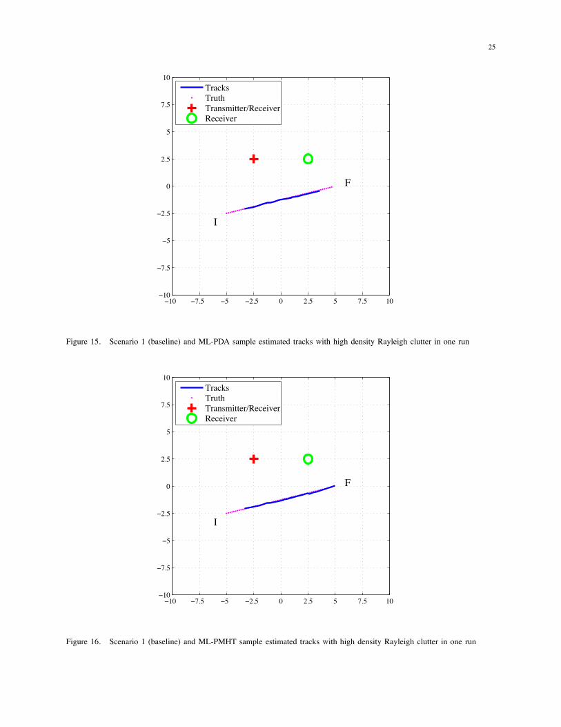
Figure 15. Scenario 1 (baseline) and ML-PDA sample estimated tracks with high density Rayleigh clutter in one run

−10 −7.5 −5 −2.5 0 2.5 5 7.5 10−10

−7.5

−5

−2.5

0

2.5

5

7.5

10


I

F

Figure 16. Scenario 1 (baseline) and ML-PMHT sample estimated tracks with high density Rayleigh clutter in one run

26

Individual examples taken from the Monte Carlo runs help to further illustrate this. For scenario

1, an ML-PDA result shown in Figure 5 and an ML-PMHT result shown in Figure 6 are virtually

indistinguishable from each other. For the same scenario with the Rayleigh clutter, results for

the two algorithms (Figure 15 for ML-PDA and Figure 16 for ML-PMHT) are also very similar.

Finally, for scenario 3, the ML-PDA example in Figure 9 and the ML-PMHT example in Figure

10 appear very much alike.

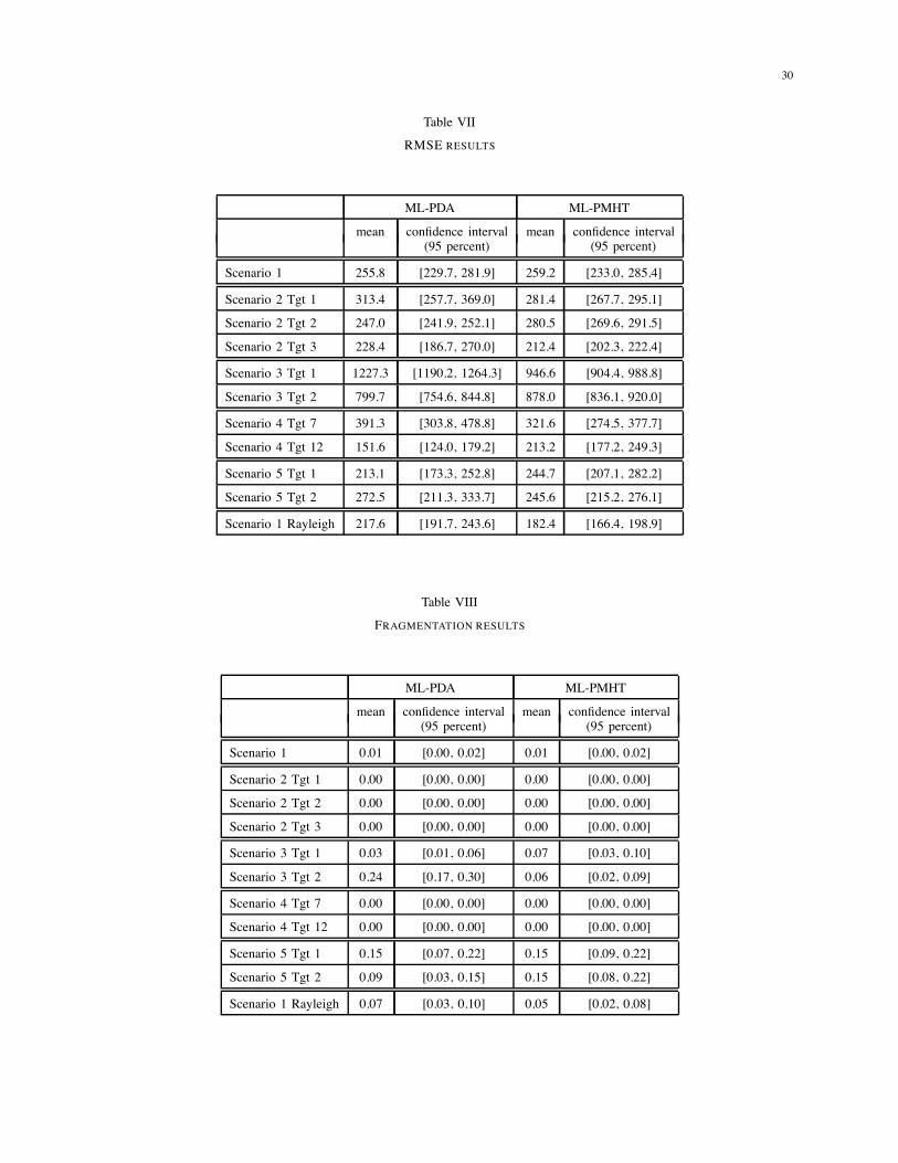
For the scenarios with targets in close proximity to each other with similar motion dynamics

(scenarios 2 and 5), or the scenario with multiple targets that were close enough to potentially

cause a tracker to switch targets (scenario 4), the results in Tables VI – XI show that ML-PMHT

clearly outperforms ML-PDA. This is due to the true multitarget implementation for ML-PMHT

in contrast to the sequential single-target tracking logic that is necessary for ML-PDA. In scenario

2, ML-PMHT is able to track targets 1 and 2 in excess of 80 percent of the time and track target

3 nearly 50 percent of the time. In contrast, ML-PDA is tracking target 2 (the middle target)

100 percent of the time, and targets 1 and 3 (the outer targets) less than 10 percent of the time.

(Overall, ML-PMHT is tracking at least one target 100 percent of the time.)

The reason ML-PDA is not performing as well as ML-PMHT in this case is the sequential

single-target implementation that is necessary for ML-PDA. Figure 17 illustrates what is hap-

pening in scenario 2. This figure shows measurements from three targets in close proximity

to each other, all moving in the same direction. For clarity of illustration, the measurements

have no noise, and there are no clutter measurements shown. ML-PDA is implemented in a

sequential mode; the first track “finds” the high-SNR measurement in each scan, and then these

measurements are excised from the data. The next track finds the remaining (relatively) high-

SNR measurement, and again, these measurements are excised from the data. Since both found

tracks are using data from all three true targets, the tracks tend to zigzag back and forth over the

middle target (and each other). As a result, the track scoring will most likely result in the middle

target being tracked by both tracks. Over many trials, this will produce a high Pd value for the

middle target, a duplicate track for the middle target, and low Pd for the outer targets. This is

exactly what is seen in the Monte Carlo results for scenario 2 — for ML-PDA the middle target

had a Pd of 100 percent, while the outer targets had a Pd of less than 10 percent. The middle

target also had, on average, 1.07 duplicate tracks associated with it.

In contrast, ML-PMHT, with its more natural and appealing true multitarget formulation, can

27

Measurements excised by track 1 Measurements excised by track 2

Track 1 Track 2

High SNR measurementMedium SNR measurementLow SNR measurement

Target Motion (for all three targets)

Figure 17. Example of multitrack measurement assignment for ML-PDA

better find all three targets. Simultaneously optimizing for multiple targets at once prevents the

“claiming” of the high-SNR measurement by the first track to run through the data; instead, the

high-SNR measurements are more equally (and correctly) divided between the three tracks, as

is shown in Figure 18. Scenario 5 showed similar results. ML-PDA was only able to track both

targets approximately 45 percent of the time, while ML-PMHT was able to track both targets

approximately 65 percent of the time. This number is actually slightly misleading; the relatively

low numbers for ML-PDA are due to the fact that tracks using this algorithm switched targets on

the portion of the trajectory where the targets were close, and the tracks ended up on the wrong

targets, driving down Pd. There was some switching for ML-PMHT as well, but as is seen by

the results, ML-PDA was more susceptible to this problem. This is a result of the sequential

single-target implementation used for ML-PDA that is described above.

Individual examples from the Monte Carlo runs again reinforce this conclusion. A scenario 2

result for ML-PDA is shown in Figure 7. Here, the first track (on the middle target) “claims”

and then excises all the high-SNR measurements. A second track is initiated, and it claims

the remaining (relatively) high-SNR measurements, in the process crossing over the first track

several times. As a result, it appears that this track would be associated with the middle target

28

Track 1 Track 2 Track 3

High SNR measurementMedium SNR measurementLow SNR measurement

Target Motion (for all three targets)

Figure 18. Example of multitrack measurement assignment for ML-PMHT

as well. There are not enough high-SNR measurements left to form a third track. In contrast,

the multitarget ML-PMHT tracker, shown in Figure 8 is able to track all three targets with a

minimum of switching. Examples from scenario 5 show similar results. In Figure 13, ML-PDA

is not able to separate the targets on the portion of the track where the two targets are paralleling

each other at very close range; during this portion, the tracks actually switch between targets five

times. In contrast, in Figure 14, the multitarget ML-PMHT tracker is able to track both targets

without any switching.

Finally, ML-PMHT outperformed ML-PDA on scenario 4 for almost all of the targets for

similar reasons. (Results from only targets 7 and 12 are shown below; they are fairly represen-

tative of all 13 targets in this scenario). Again, the sequential single target tracking framework

for ML-PDA could not perform as well as the true multitarget implementation for ML-PMHT.

Tracks using the ML-PDA implementation were far more susceptible to being drawn off from

one target to another by high-SNR measurements (similar to the effect illustrated in Figure 17).

Compare the performance of ML-PDA on this scenario in Figure 11 with the performance of

ML-PMHT in Figure 12. Several instances of track switching are visible in the ML-PDA plot

that are not seen in the ML-PMHT plot. While this switching is not between targets with similar

29

Table VI

IN-TRACK PERCENTAGE RESULTS

ML-PDA ML-PMHT

mean confidence interval mean confidence interval(95 percent) (95 percent)

Scenario 1 95.4 [94.8, 96.0] 95.4 [94.8, 96.0]

Scenario 2 Tgt 1 12.0 [7.5, 16.6] 83.9 [79.6, 88.2]

Scenario 2 Tgt 2 100 [100, 100] 87.5 [83.7, 91.3]

Scenario 2 Tgt 3 1.9 [0.0, 3.8] 53.1 [46.5, 59.7]

Scenario 3 Tgt 1 82.7 [81.0, 84.4] 82.5 [81.0, 84.0]

Scenario 3 Tgt 2 76.1 [74.2, 78.0] 77.1 [75.4, 78.9]

Scenario 4 Tgt 7 61.0 [54.7, 67.4] 91.1 [89.3, 92.8]

Scenario 4 Tgt 12 52.5 [45.9, 59.2] 96.3 [95.9, 96.8]

Scenario 5 Tgt 1 45.3 [38.4, 52.2] 63.1 [56.5, 69.7]

Scenario 5 Tgt 2 48.4 [41.5, 55.4] 63.7 [57.1, 70.2]

Scenario 1 Rayleigh 66.9 [66.0, 67.8] 67.4 [66.6, 68.3]

dynamics (as happens with Scenarios 2 and 5), it is happening with targets that are moving very

slowly. As as result, there are no dynamics — either evolving position over time or Doppler —

to differentiate measurements between two targets.

All the simulations up to this point were performed using the ML-PDA target measurement

generation model — that is, at most one measurement was generated by the target in any given

scan. In this condition, ML-PMHT and ML-PDA had identical performance in the single-target

cases, and ML-PMHT outperformed ML-PDA in the small-separation multitarget cases. We now

round out the comparison between the two algorithms by considering what happens when the

ML-PMHT target measurement generation model is used to generate the data and more than

one measurement is allowed to originate from the target.

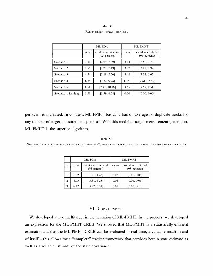
In order to do this, Scenario 1 (with K-distributed clutter) was re-run for one, two and three

expected target returns per scan. Results for all metrics were virtually the same between the

algorithms (and similar to results shown above for Scenario 1), with the exception of the number

of duplicate tracks. These results are shown in Table XII. Here, ML-PDA, as expected, suffers

from an increasing number of duplicate tracks as N , the expected number of target measurements

30

Table VII

RMSE RESULTS

ML-PDA ML-PMHT


Scenario 1 255.8 [229.7, 281.9] 259.2 [233.0, 285.4]

Scenario 2 Tgt 1 313.4 [257.7, 369.0] 281.4 [267.7, 295.1]

Scenario 2 Tgt 2 247.0 [241.9, 252.1] 280.5 [269.6, 291.5]

Scenario 2 Tgt 3 228.4 [186.7, 270.0] 212.4 [202.3, 222.4]

Scenario 3 Tgt 1 1227.3 [1190.2, 1264.3] 946.6 [904.4, 988.8]

Scenario 3 Tgt 2 799.7 [754.6, 844.8] 878.0 [836.1, 920.0]

Scenario 4 Tgt 7 391.3 [303.8, 478.8] 321.6 [274.5, 377.7]

Scenario 4 Tgt 12 151.6 [124.0, 179.2] 213.2 [177.2, 249.3]

Scenario 5 Tgt 1 213.1 [173.3, 252.8] 244.7 [207.1, 282.2]

Scenario 5 Tgt 2 272.5 [211.3, 333.7] 245.6 [215.2, 276.1]


Table VIII

FRAGMENTATION RESULTS

ML-PDA ML-PMHT


Scenario 1 0.01 [0.00, 0.02] 0.01 [0.00, 0.02]

Scenario 2 Tgt 1 0.00 [0.00, 0.00] 0.00 [0.00, 0.00]

Scenario 2 Tgt 2 0.00 [0.00, 0.00] 0.00 [0.00, 0.00]

Scenario 2 Tgt 3 0.00 [0.00, 0.00] 0.00 [0.00, 0.00]

Scenario 3 Tgt 1 0.03 [0.01, 0.06] 0.07 [0.03, 0.10]

Scenario 3 Tgt 2 0.24 [0.17, 0.30] 0.06 [0.02, 0.09]

Scenario 4 Tgt 7 0.00 [0.00, 0.00] 0.00 [0.00, 0.00]

Scenario 4 Tgt 12 0.00 [0.00, 0.00] 0.00 [0.00, 0.00]

Scenario 5 Tgt 1 0.15 [0.07, 0.22] 0.15 [0.09, 0.22]

Scenario 5 Tgt 2 0.09 [0.03, 0.15] 0.15 [0.08, 0.22]


31

Table IX

DUPLICATE TRACK RESULTS

ML-PDA ML-PMHT


Scenario 1 0.18 [0.13, 0.24] 0.02 [0.00, 0.04]

Scenario 2 Tgt 1 0.00 [0.00, 0.00] 0.04 [0.01, 0.08]

Scenario 2 Tgt 2 1.07 [1.01, 1.14] 0.48 [0.39, 0.57]

Scenario 2 Tgt 3 0.00 [0.00, 0.00] 0.00 [0.00, 0.00]

Scenario 3 Tgt 1 0.03 [0.01, 0.06] 0.07 [0.03, 0.10]

Scenario 3 Tgt 2 0.24 [0.17, 0.30] 0.06 [0.02, 0.09]

Scenario 4 Tgt 7 0.00 [0.00, 0.00] 0.09 [0.05, 0.13]

Scenario 4 Tgt 12 0.09 [0.03, 0.14] 0.18 [0.12, 0.24]

Scenario 5 Tgt 1 0.04 [0.00, 0.08] 0.13 [0.07, 0.19]

Scenario 5 Tgt 2 0.02 [0.00, 0.05] 0.11 [0.05, 0.16]


Table X

FALSE TRACK RESULTS

ML-PDA ML-PMHT


Scenario 1 0.07 [0.03, 0.11] 0.07 [0.03, 0.11]

Scenario 2 0.06 [0.03, 0.09] 0.15 [0.15, 0.21]

Scenario 3 0.34 [0.26, 0.42] 0.26 [0.19, 0.33]

Scenario 4 0.17 [0.10, 0.23] 0.14 [0.09, 0.20]

Scenario 5 2.13 [1.92, 2.34] 2.65 [2.44, 2.86]


32

Table XI

FALSE TRACK LENGTH RESULTS

ML-PDA ML-PMHT


Scenario 1 3.14 [2.59, 3.69] 3.14 [2.56, 3.73]

Scenario 2 2.75 [2.31, 3.19] 3.37 [2.81, 3.92]

Scenario 3 4.34 [3.18, 5.50] 4.42 [3.32, 5.62]

Scenario 4 6.75 [3.72, 9.78] 11.67 [7.81, 15.52]

Scenario 5 8.98 [7.81, 10.16] 8.55 [7.59, 9.51]


per scan, is increased. In contrast, ML-PMHT basically has on average no duplicate tracks for

any number of target measurements per scan. With this model of target-measurement generation,

ML-PMHT is the superior algorithm.

Table XII

NUMBER OF DUPLICATE TRACKS AS A FUNCTION OF N , THE EXPECTED NUMBER OF TARGET MEASUREMENTS PER SCAN

ML-PDA ML-PMHT

N mean confidence interval mean confidence interval(95 percent) (95 percent)

1 1.32 [1.21, 1.43] 0.03 [0.00, 0.05]

2 4.05 [3.88, 4.23] 0.04 [0.01, 0.06]

3 6.12 [5.92, 6.31] 0.09 [0.05, 0.13]

VI. CONCLUSIONS

We developed a true multitarget implementation of ML-PMHT. In the process, we developed

an expression for the ML-PMHT CRLB. We showed that ML-PMHT is a statistically efficient

estimator, and that the ML-PMHT CRLB can be evaluated in real time, a valuable result in and

of itself – this allows for a “complete” tracker framework that provides both a state estimate as

well as a reliable estimate of the state covariance.

33

We then tested these developments by comparing ML-PDA and ML-PMHT with Monte Carlo

testing. This testing first showed that ML-PDA and ML-PHMT are effective very low observable

trackers, working down to an expected target SNR of 4-5 dB (post signal processing). After this,

the ML-PDA and the ML-PMHT tracking algorithms were applied to five different benchmark

scenarios with Monte Carlo trials using a target measurement generation model of zero or one

measurements originating from the target in a scan. For scenarios with a single target or multiple

targets with measurements that could easily be differentiated by dynamics, the performances of

ML-PDA and ML-PMHT were identical — ML-PMHT did not suffer from the fact that its

measurement assignment model did not match the actual target measurement generation model.

In cases with closely-spaced targets with measurements that could not be differentiated easily

by dynamics, ML-PMHT outperformed ML-PDA due to the fact that the former had a true

multitarget LLR formulation, while the latter had to handle multiple targets in a sequential

single-target mode. Finally, when the target measurement generation model was switched to

that of ML-PMHT, with multiple measurements per scan being generated by the target, ML-

PMHT outperformed ML-PDA in terms of the number of duplicate tracks generated. Overall,

the performance of ML-PMHT makes it the preferred algorithm.

APPENDIX A

CALCULATION OF THE ML-PMHT FISHER INFORMATION MATRIX

Here we fully derive the Fisher Information Matrix (FIM) for a window of ML-PMHT data.

This is a specific implementation of the general work given in [22]. The derivation is also similar

to that done for ML-PDA in [8]. However, the ML-PMHT calculation ends up being at most a

4-fold integral (as opposed to approximately an m-fold integral for ML-PDA, where m is the

number of measurements in a scan), so this can be done real-time instead of having to calculate

it offline with Monte-Carlo integration as must be done with ML-PDA.

Consider a window of ML-PMHT data with Nw scans. Since all measurements from scan to

scan are assumed to be independent, the FIM J of the total window can just be written as the

sum of the FIM’s Ji of the individual scans,

J =

Nw∑i=1

Ji (29)

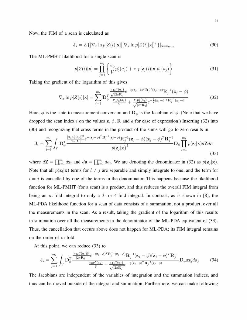
34

Now, the FIM of a scan is calculated as

Ji = E{[∇x ln p[Z(i)|x]][∇x ln p[Z(i)|x]]T}|x=xtrue (30)

The ML-PMHT likelihood for a single scan is

p[Z(i)|x] =mi∏j=1

{π0

Vpτ0(aj) + π1p[zj(i)|x]pτ1(aj)

}(31)

Taking the gradient of the logarithm of this gives

∇x ln p[Z(i)|x] =mi∑j=1

DTφ


e−12(zj−φ)TR−1

j (zj−φ)R−1j (zj − φ)

π0pτ0(aj )

V+



j (zj−φ)(32)

Here, φ is the state-to-measurement conversion and Dφ is the Jacobian of φ. (Note that we have

dropped the scan index i on the values z, φ, R and a for ease of expression.) Inserting (32) into

(30) and recognizing that cross terms in the product of the sums will go to zero results in

Ji =

mi∑j=1

∫V

DTφ

[π1pτ1(aj)]2



p(zj|x)2 Dφ

mi∏l=1

p(zl|x)dZda(33)

where dZ =∏mi

l=1 dzl and da =∏mi

l=1 dal. We are denoting the denominator in (32) as p(zj|x).Note that all p(zl|x) terms for l �= j are separable and simply integrate to one, and the term for

l = j is cancelled by one of the terms in the denominator. This happens because the likelihood

function for ML-PMHT (for a scan) is a product, and this reduces the overall FIM integral from

being an m-fold integral to only a 3- or 4-fold integral. In contrast, as is shown in [8], the

ML-PDA likelihood function for a scan of data consists of a summation, not a product, over all

the measurements in the scan. As a result, taking the gradient of the logarithm of this results

in summation over all the measurements in the denominator of the ML-PDA equivalent of (33).

Thus, the cancellation that occurs above does not happen for ML-PDA; its FIM integral remains

on the order of m-fold.

At this point, we can reduce (33) to

Ji =

mi∑j=1

∫V

DTφ

[π1pτ1(aj )]2



π0pτ0 (aj)

V+

π1pτ1(aj)√|2πRj |


j (zj−φ)Dφdzjdaj (34)

The Jacobians are independent of the variables of integration and the summation indices, and

thus can be moved outside of the integral and summation. Furthermore, we can make following

35

substitution of

ξj = Gj(zj − φ) (35)

where Gj is the Cholesky decomposition of R−1j such that GT

j Gj = R−1j . With this, it is

possible to write the final expression for Ji:

Ji = DTφ

mi∑j=1

GTj

∫V

[π1pτ1(aj )]2

|2πRj | e−ξTj ξjξjξTj

π0pτ0(aj )

V+


e−12ξTj ξj

dξjdajGj

|Gj |Dφ (36)

This is a relatively simple 3- or 4-fold integration (depending on the dimension of z j) in this

application and can be done in real time. The resultant Ji for each scan is simply summed up

then in accordance with (29) to get the FIM for a window of data.

REFERENCES

[1] S. Schoenecker, P. Willett, and Y. Bar-Shalom, “A comparison of the ML-PDA and the ML-PMHT algorithms,” in Proc.

of 14th Intern’l Conf. on Info. Fusion, Chicago, IL, 2011.

[2] ——, “Maximum likelihood probabilistic multi-hypothesis tracker applied to multistatic sonar data sets,” in Proc. SPIE

Conf. on Signal Processing, Sensor Fusion, and Target Recognition, Orlando, FL, 2011.

[3] C. Jauffret and Y. Bar-Shalom, “Track formation with bearing and frequency measurements in clutter,” in Proc. of the 29th

Conf. on Decision and Control, Honolulu, HI, December 1990.

[4] W. Blanding, P. Willett, and S. Coraluppi, “Sequential ML for multistatic sonar tracking,” in Proc. Oceans 2007 Europe

Conf., Aberdeen, Scotland, June 2007.

[5] P. Willett and S. Coraluppi, “Application of the MLPDA to bistatic sonar,” in Proc. of IEEE Aerosp. Conf., Big Sky, MT,

March 2005.

[6] ——, “MLPDA and MLPMHT applied to some MSTWG data,” in Proc. 9th Intern’l Conf. on Info. Fusion, Florence,

Italy, July 2006.

[7] Y. Bar-Shalom, P. Willett, and X. Tian, “The ML-PDA estimator for VLO targets,” in Tracking and Data Fusion: A

Handbook of Algorithms. YBS Publishing, 2011, ch. 3.8.1, 3.8.2, pp. 209–212.

[8] T. Kirubarajan and Y. Bar-Shalom, “Low observable target motion analysis using amplitude information,” IEEE Trans. on

Aerosp. and Electronic Syst., vol. 32, no. 4, pp. 1637–1382, 1996.

[9] M. R. Chummun, Y. Bar-Shalom, and T. Kirubarajan, “Adaptive early-detection ML-PDA estimator for LO targets with

EO sensors,” IEEE Trans. on Aerosp. and Electronic Syst., vol. 38, no. 2, pp. 694–707, 2002.

[10] W. Blanding, P. Willett, and Y. Bar-Shalom, “ML-PDA: Advances and a new multitarget approach,” EURASIP Journal on

Advances in Signal Processing, vol. 2008, pp. 1–13, 2008.

[11] ——, “Offline and real-time methods for ML-PDA track validation,” IEEE Trans. on Signal Processing, vol. 55, no. 5,

pp. 1994–2006, 2007.

[12] R. Georgescu, P. Willett, and S. Schoenecker, “GM-CPHD and MLPDA applied to the SEABAR07 and TNO-blind multi-

static sonar data,” in Proc. of 12th Intern’l Conf. on Info. Fusion, Seattle, WA, 2009.

36

[13] ——, “GM-CPHD and ML-PDA applied to the Metron multi-static sonar dataset,” in Proc. of 13th Intern’l Conf. on Info.

Fusion, Edinburgh, Scotland, 2010.

[14] A. Dempster, N. Laird, and D. Rubin, “Maximum likelihood from incomplete data via the EM algorithm,” Journal of the

Royal Statistical Society, Series B (Methodological), vol. 39, no. 1, pp. 1–38, 1977.

[15] S. Coraluppi, “Mulitstatic sonar localization,” IEEE Journal of Oceanic Engineering, vol. 31, no. 4, pp. 964–974, 2006.

[16] H. Cox, “Fundamentals of bistatic active sonar,” BBN Systems and Technologies Corporation, Tech. Rep. W1038, 1988.

[17] Y. Bar-Shalom, X. R. Li, and T. Kirubarajan, “Definition and the statistical tests for filter consistency,” in Estimation with

Applications to Tracking and Navigation. John Wiley and Sons, Inc., 2001, ch. 5.4.2, 5.4.3, pp. 234–240.

[18] P. Willett. (2012, August) University of Connecticut Department of Electrical & Computer Engineering website. [Online].

Available: http://www.engr.uconn.edu/∼willett/current papers/

[19] D. Abraham, “Detection-threshold approximation for non-Gaussian backgrounds,” IEEE Journal of Oceanic Engineering,

vol. 35, no. 2, pp. 355–365, 2010.

[20] D. Abraham and A. Lyons, “Simulation of non-Rayleigh reverberation and clutter,” IEEE Journal of Oceanic Engineering,

vol. 29, no. 2, pp. 347–362, 2004.

[21] A. Abramowitz and I. Stegun, “Handbook of mathematical functions,” in National Bureau of Standards, Applied Math.

Series, ser. 55. Dover Publications, 1965, ch. 9.1.1, 9.1.98, and 9.12.

[22] Y. Ruan, P. Willett, and R. Streit, “A comparison of the PMHT and PDAF tracking algorithms based on their model

CRLBs,” in Proc. SPIE Aerosense Conf. on Acquisition, Tracking and Pointing, Orlando, FL, 1999.

1 ml-pda and ml-pmht: comparing multistatic sonar...

Documents