probabilistic analysis of a large-scale urban trafï¬c
TRANSCRIPT

Probabilistic Analysis of a Large-Scale Urban TrafficSensor Data Set
Jon Hutchins ∗
Dept. of Computer ScienceUniversity of California, Irvine
Alexander IhlerDept. of Computer Science
University of California, IrvineCA 96297-3435
Padhraic SmythDept. of Computer Science
University of California, IrvineCA 96297-3435
ABSTRACTReal-world sensor time series are often significantly noisierand more difficult to work with than the relatively cleandata sets that tend to be used as the basis for experimentsin many research papers. In this paper we report on a largecase-study involving statistical data mining of over 300 mil-lion measurements from 1700 freeway traffic sensors over aperiod of seven months in Southern California. We discussthe challenges posed by the wide variety of different sensorfailures and anomalies present in the data. The volume andcomplexity of the data precludes the use of manual visu-alization or simple thresholding techniques to identify theseanomalies. We describe the application of probabilistic mod-eling and unsupervised learning techniques to this data setand illustrate how these approaches can successfully detectunderlying systematic patterns even in the presence of sub-stantial noise and missing data.
Categories and Subject DescriptorsI.5 [Pattern Recognition]: Statistical Models; I.2.6 [ArtificialIntelligence]: Learning—graphical models
General Termsprobabilistic modeling, traffic model, large-scale analysis,case study
Keywordsloop sensors, MMPP, traffic, Poisson
1. INTRODUCTIONLarge-scale sensor instrumentation is now common in a vari-ety of applications including environmental monitoring, in-dustrial automation, surveillance and security. As one exam-ple, the California Department of Transportation (Caltrans)maintains an extensive network of over 20,000 inductive loopsensors on California freeways [1, 7]. Every 30 seconds each
∗contact information: (949) 232-7405
of these traffic sensors reports a count of the number of vehi-cles that passed over the sensor and the percentage of timethe sensor was covered by a vehicle, measurements knownas the flow and occupancy respectively. The data are con-tinuously archived, providing a potentially rich source fromwhich to extract information about urban transportationpatterns, traffic flow, accidents, and human behavior in gen-eral.
Large-scale loop sensor data of this form are well knownto transportation researchers, but have resisted systematicanalysis due to the significant challenges of dealing withnoisy real-world sensor data at this scale. Bickel et al. [1]outline some of the difficulties in a recent survey paper:
...loop data are often missing or invalid...a loopdetector can fail in various ways even when it re-ports values...Even under normal conditions, themeasurements from loop detectors are noisy...
Bad and missing samples present problems forany algorithm that uses the data for analysis...weneed to detect when data are bad and discardthem
A systematic and principled algorithm [for de-tecting faulty sensors] is hard to develop mainlydue to the size and complexity of the problem.An ideal model needs to work well with thou-sands of detectors, all with potentially unknowntypes of malfunction.
Even constructing a training set is not trivialsince there is so much data to examine and itis not always possible to be absolutely sure if thedata are correct even after careful visual inspec-tion.
Similar issues arise in many large real-world sensor systems.In particular, the presence of “bad” sensor data is a persis-tent problem—sensors are often in uncontrolled and rela-tively hostile environments, subject to a variety of unknownand unpredictable natural and human-induced changes. Re-search papers on sensor data mining and analysis often payinsufficient attention to these types of issues; for example,our previous work [4, 5] did not address sensor failures di-rectly. However, if research techniques and algorithms forsensor data mining are to be adapted and used for real-worldproblems it is essential that they can handle the challengesof such data in a robust manner.

DEC JAN FEB MAR APR MAY JUN
0
20
40
60
80
veh c
ount
MON TUE WED THU FRI
0
20
40
60
80
veh c
ount
(a)
(b)
Figure 1: (a) A sensor that is stuck at zero for almosttwo months. (b) Five days of measurements at theend of the period of sensor failure, after which atypical pattern of low evening activity and higheractivity at morning and afternoon rush hour beginsto appear.
DEC JAN FEB MAR APR MAY JUN0
50
100
150
ve
h c
ou
nt
SAT SUN MON TUE WED THU FRI0
50
100
150
ve
h c
ou
nt
SAT SUN MON TUE WED THU FRI0
50
100
150
ve
h c
ou
nt
(a)
(b)
(c)
Figure 2: (a) A sensor with normal (periodic) ini-tial behavior, followed by large periods of missingdata and suspicious measurements. (b) A week atthe beginning of the study showing the periodic be-havior typical of traffic. (c) A week in February.Other than the missing data, these values may notappear that unusual. However, they are not consis-tent with the much clearer pattern seen in the firsttwo months. The presence of unusually large spikesof traffic, particularly late at night, also make thesemeasurements suspicious.
In this paper we present a case study of applying probabilis-tic sensor modeling algorithms to a data set with 2263 loopsensors involving over 100 million measurements, recordedover seven months in Southern California. The sensor mod-eling algorithms are based on unsupervised learning tech-niques that simultaneously learn the regular patterns of hu-man behavior from data as well as the occurrence of unusualevents, as described in our previous work [4, 5].
The seven months of time-series data from the 2263 loopsensors contain a wide variety of anomalous behavior in-
cluding “stuck at zero” failures, missing data, suspiciouslyhigh readings, and more. Figure 1 shows a sensor with a“stuck at zero” failure, and Figure 2 shows an example of asensor with extended periods both of missing data and ofsuspicious measurements. In this paper we focus specificallyon the challenges involved in working with large numbers ofsensors having diverse characteristics. Removing bad datavia visual inspection is not feasible given the number of sen-sors and measurements, notwithstanding the fact that it canbe non-trivial for a human to visually distinguish good datafrom bad. In Figure 2, for example, the series of measure-ments between January and March might plausibly pass fordaily traffic variations if we did not know the normal con-ditions. Figure 2 also illustrates why simple thresholdingtechniques are generally inadequate, due to the large vari-ety in patterns of anomalous sensor behavior.
We begin by illustrating the results of a probabilistic modelthat does not include any explicit mechanism for handlingsensor failures. As a result, the unsupervised learning algo-rithms fail to learn a pattern of normal behavior for a largenumber of sensors. We introduce a relatively simple mecha-nism into the model to account for sensor failures, resultingin a significant increase in the number of sensors where atrue signal can be reliably detected, as well as improved au-tomatic identification of sensors that are so inconsistent asto be unmodelable. The remainder of the paper illustrateshow the inferences made by the fault-tolerant model canbe used for a variety of analyses, clearly distinguishing (a)the predictable hourly, daily, and weekly rhythms of humanbehavior, (b) unusual bursts of event traffic activity (for ex-ample, due to sporting events or traffic accidents), and (c)sequences of time when the sensor is faulty. We concludethe paper with a discussion of lessons learned from this casestudy.
2. LOOP SENSOR DATAWe focus on the flow measurements obtained from eachloop sensor, defined as the cumulative count of vehicles thatpassed over the sensor. The flow is reported and reset every30 seconds, creating a time series of count data. As shown inFigures 1 and 2, the vehicle count data is a combination of a“true” periodic component (e.g., Figure 2(b)) and a varietyof different types of failures and noise.
We collected flow measurements between November 26, 2006and July 7, 2007 for all of the entrance and exit ramps inLos Angeles and Orange County. The data were downloadedvia ftp from the PeMS database [1, 7] maintained by U.C.Berkeley in cooperation with Caltrans. Of the 2263 loopsensors, 566 sensors reported missing (no measurement re-ported) or zero values for the entire duration of the sevenmonth study. The remaining 1716 sensors reported missingmeasurements 29% of the time on average. Missing data oc-curred either when PeMS did not report a measurement dueto a faulty detector or a faulty collection system, or whenour own system was unable to access PeMS.
Aside from missing measurements and sensor failures, theperiodic structure in the data reflecting normal (predictable)driving habits of people can be further masked by periodsof unusual activity [5]; including those caused by traffic ac-cidents or large events such as concerts and sporting events.

Time t+1
������������ ������������
Time t-1 Time t
ObservedMeasurement
ObservedMeasurement
ObservedMeasurement
Poisson Rate �(t-1)
Poisson Rate �(t+1)
Poisson Rate �(t)
NormalCount
NormalCount
EventCount
EventCount
EventCount
Event Event Event
NormalCount
Figure 3: Graphical model of the original approachproposed in [4, 5]. Both the event and rate variablescouple the model across time: the Markov eventprocess captures rare, persistent events, while thePoisson rate parameters are linked between similartimes (arrows not shown). For example, the rate ona particular Monday during the 3:00 to 3:05pm timeslice is linked to all other Mondays at that time.
6:00am 12:00pm 6:00pm
20
40
veh
coun
t
00.5
1
p(E
)
Figure 4: Example inference results with the modelfrom FIgure 3. The blue line shows actual flow mea-surements for one sensor on one day, while the blackline is the model’s inferred rate parameters for thenormal (predictable) component of the data. Thebar plot below shows the estimated probability thatan unusual event is taking place.
Noisy measurements, missing observations, unusual eventactivity, and multiple causes of sensor failure combine tomake automated analysis of a large number of sensors quitechallenging.
3. ORIGINAL MODELIn Ihler et al. [5] we presented a general probabilistic model(hereafter referred to as the original model) that learns pat-terns of human behavior that is hidden in time series of countdata. The model was tested on two real-world data sets, andwas shown to be significantly more effective than a baselinemethod at discovering both underlying recurrent patterns ofhuman behavior as well as finding and quantifying periodsof unusual activity. Our original model consisting of twocomponents: (a) a time-varying Poisson process that canaccount for recurrent patterns of behavior, and (b) an ad-ditional “bursty” Poisson process, modulated by a Markovprocess, that accounts for unusual events.
If labeled data are available (i.e. we have prior knowledgeof the time periods when unusual events occur), then esti-mation of this model is straightforward. However, labeleddata are difficult to obtain and are likely to be only partiallyavailable even in a best-case scenario. Even with close vi-sual inspection it is not always easy to determine whetheror not event activity is present. Supervised learning (usinglabeled data) is even less feasible when applying the modelto a group of 1716 sensors.
Instead, the approach we proposed in [4, 5] separates thenormal behavior and the unusual event behavior using anunsupervised Markov modulated Poisson process [9, 10].The graphical model is shown in Figure 3. The normal (pre-dictable) component of the data is modeled using a time-varying Poisson process, and the unusual event activity ismodeled separately using a Markov chain. The event vari-able can be in one of three states: no event, positive event(indicating unusually high activity), or negative event (un-usually low activity).
In the model, the Poisson rate parameter defines how thenormal, periodic behavior counts are expected to vary, whilethe Markov chain component allows unusual events to havepersistence. If the observed measurement is far from therate parameter, or if event activity has been predicted in theprevious time slice, the probability of an event increases.
Given the model and the observed historical counts, we caninfer the unknown parameters of the model (such as the rateparameters of the underlying normal traffic pattern) as wellas the values of the hidden states. Note that in addition tothe event state variables being connected in time, the rateparameters λ(t) are also linked (not shown in Figure 3).This leads to cycles in the graphical model, making exactinference intractable. Fortunately, there are approximationalgorithms that are effective in practice. As described in [4,5], we use a Gibbs sampler [3] for learning the hidden pa-rameters and hidden variables. The algorithm uses standardhidden Markov recursions with a forward inference pass fol-lowed by a backwards sampling pass for each iteration ofthe sampler. The computational complexity of the sampleris linear in the number of time slices, and empirically con-vergence is quite rapid (see [5] for more details).
Figure 4 shows an example of the results of the inference pro-cedure. The measured vehicle count for this particular dayfollows the model’s inferred time-varying Poisson rate for thenormal (predictable) component of the data for most of theday. In the evening, however, the observed measurementsdeviate significantly. This deviation indicates the presenceof unusual event activity and is reflected in the model’s esti-mated event probability (bottom panel). The output of themodel also includes information about the magnitude andduration of events.
The event activity in this example looks obvious given theinferred profile of normal behavior; however, simultaneouslyidentifying the normal pattern and unusual event activityhidden within the measurements is non-trivial. In our earlierwork [4, 5] we found that the Markov-modulated Poissonprocess was significantly more accurate at detecting knownevents than simpler baseline methods such as threshold-type

Event Fraction Number of Sensors0 to 10% 91210 to 20% 38620 to 50% 26550 to 100% 153
Table 1: Original model’s fit. The study’s 1716 sen-sors are categorized using a measure of the model’sability to find a predictable periodic component inthe sensor measurements (if present). The eventfraction is defined as the fraction of time a sensor’smeasurements are classified as a positive or negativeevent. For sensors higher in the table, the model hasfound a strong periodic component with fewer peri-ods of unusual event activity.
MON TUE WED THU FRI0
0.51
Time
P(E
)
MON TUE WED THU FRI
0
20
40
60
80
veh
coun
t
Figure 5: Original model output for the sensor inFigure 1. Shown are the observed measurements(blue) for one week (the same week as Figure 1(b))along with the model’s inferred Poisson rate (black).With a long period stuck at zero, a poor model is in-ferred for normal behavior in the middle of the day.This is reflected in the event probabilities (bottom),where unusual event activity is predicted for mostof each day.
detectors based on Poisson models.
4. SCALE-UP CHALLENGESAfter the initial successes described in Section 3, we wantedto test the model on a much larger network of sensors.The model can generally be applied to various types of sen-sors which record count data, but the loop sensor data setwas a particularly appealing choice for our case study. Asmentioned earlier, we had access to the measurements of2263 loop sensors in the Southern California area. We alsohad additional information about the sensors that couldprove useful during analysis, such as geographic locationand whether each sensor was on an exit or entrance ramp.In addition, there are many data analysis problems specificto traffic data, including accident detection, dynamic popu-lation density estimation, and others. In our work we weremotivated by the challenge of extracting useful informationfrom this large data set to provide a basic framework foraddressing these questions.
We applied the original model to the data from our sevenmonth study involving 1716 sensors and over 300 millionhidden variables. The model was subjected to much greater
levels of variability than experienced in our earlier studies.Several weaknesses of the original model were identified asa result.
Table 1 shows one method for judging how well the modelfit the data. The table shows the fraction of time that themodel inferred unusual event activity for each of the sensorsduring our seven month study, i.e. the fraction of time slicesin which the event variable in Figure 3 was inferred to bein an unusual event state and are thus not explained by theperiodic component of the data.
There is reason to be suspicious when the model infers un-usual event activity for a large fraction of the time, especiallyin cases where unusual event activity is more common thannormal activity (as in the last row of the table). A review ofthe sensors where event activity was inferred over 50% of thetime revealed some weaknesses of the original model. Somesensors in this category were apparently faulty throughoutthe study. Another group of sensors recorded non-missingmeasurements for only a very small fraction of the study,which were not enough to form a good model. However,there were many sensors which appeared to have an un-derlying periodic behavior pattern that was missed by theoriginal model.
The sensor with the “stuck at zero” failure (Figure 1) is anexample of a sensor with a clear periodic pattern that theoriginal model missed. Figure 5 shows the model’s attemptto fit the data from this sensor. The model is able to learnearly morning and late night behavior, but an inaccurateprofile is inferred for normal behavior in the middle of theday. Examples such as this were observed across many othersensors, and in many cases where a poor model was inferredfor normal behavior there appeared to be long periods wherethe sensor was faulty.
We experimented with a number of modifications to themodel, including adjusting the priors on the parameters ofthe Markov process, avoiding poor initialization of the Gibbssampler which sometimes occurred when extensive periodsof failure were present, and dealing with missing data dif-ferently. These adjustments improved the performance ofthe model in some cases. But in many cases (particularly insensors with extensive periods of sensor failure) inaccurateprofiles were still inferred for normal behavior.
5. FAULT-TOLERANT MODELIt is clear from Section 4 that in order to make the originalmodel more general and robust, sensor failures should beaddressed directly instead of bundling them together withunusual event activity. We note that heuristic approachesto sensor fault detection in traffic data have been developedin prior work [2, 6], but these techniques are specific to loopdetectors and to certain types of sensor failures. Our focusin this paper is developing an approach that can handle moregeneral types of faults, not only in loop sensor data but alsoin other sensors that measure count data.
One possible approach to solve these problems would be tomodify the model to broaden the definition of “events” toinclude sensor failures. However, sensor failures and events(as we define them) tend to have quite different characteris-
Time t+1
������������ ������������
Time t-1 Time t
ObservedMeasurement
ObservedMeasurement
ObservedMeasurement
Poisson Rate �(t-1)
NormalCount
Poisson Rate �(t+1)
Poisson Rate �(t)
NormalCount
NormalCount
EventCount
EventCount
EventCount
Event EventEvent
Fault Fault Fault
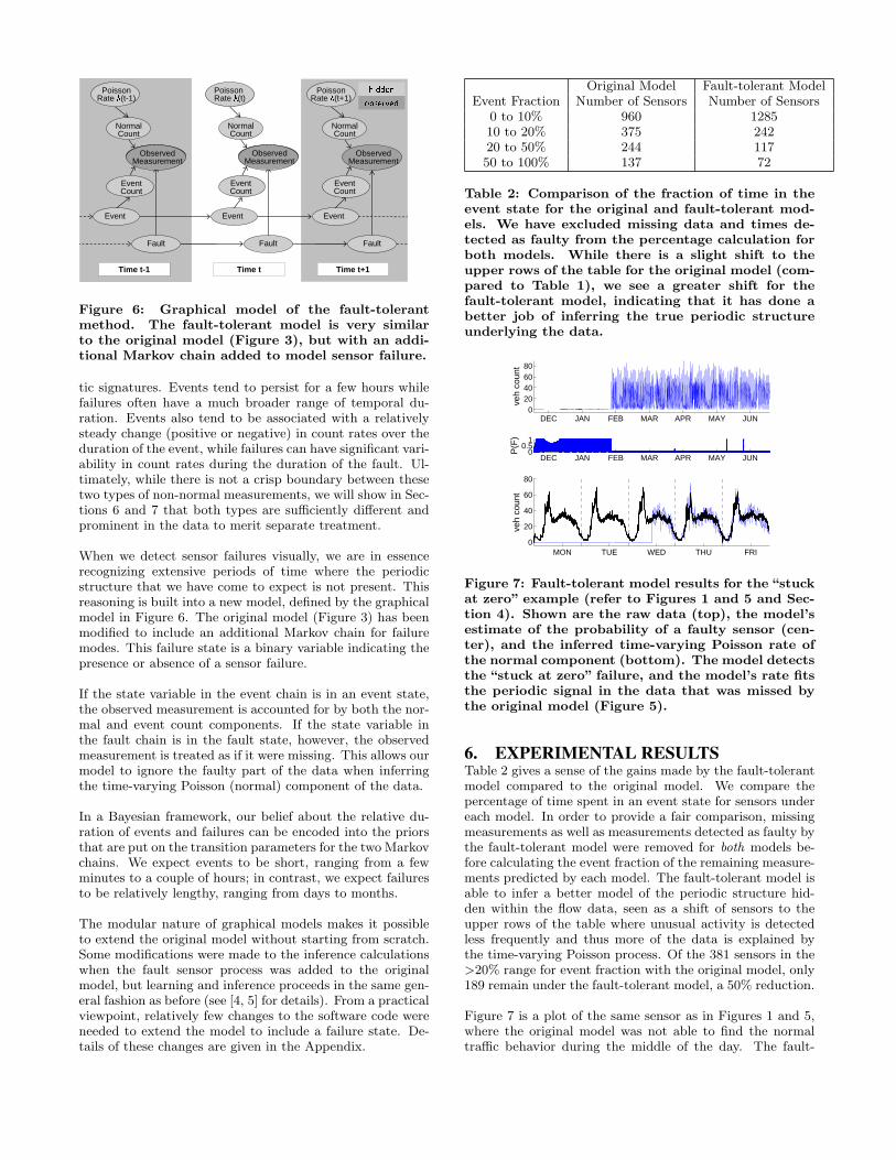
Figure 6: Graphical model of the fault-tolerantmethod. The fault-tolerant model is very similarto the original model (Figure 3), but with an addi-tional Markov chain added to model sensor failure.
tic signatures. Events tend to persist for a few hours whilefailures often have a much broader range of temporal du-ration. Events also tend to be associated with a relativelysteady change (positive or negative) in count rates over theduration of the event, while failures can have significant vari-ability in count rates during the duration of the fault. Ul-timately, while there is not a crisp boundary between thesetwo types of non-normal measurements, we will show in Sec-tions 6 and 7 that both types are sufficiently different andprominent in the data to merit separate treatment.
When we detect sensor failures visually, we are in essencerecognizing extensive periods of time where the periodicstructure that we have come to expect is not present. Thisreasoning is built into a new model, defined by the graphicalmodel in Figure 6. The original model (Figure 3) has beenmodified to include an additional Markov chain for failuremodes. This failure state is a binary variable indicating thepresence or absence of a sensor failure.
If the state variable in the event chain is in an event state,the observed measurement is accounted for by both the nor-mal and event count components. If the state variable inthe fault chain is in the fault state, however, the observedmeasurement is treated as if it were missing. This allows ourmodel to ignore the faulty part of the data when inferringthe time-varying Poisson (normal) component of the data.
In a Bayesian framework, our belief about the relative du-ration of events and failures can be encoded into the priorsthat are put on the transition parameters for the two Markovchains. We expect events to be short, ranging from a fewminutes to a couple of hours; in contrast, we expect failuresto be relatively lengthy, ranging from days to months.
The modular nature of graphical models makes it possibleto extend the original model without starting from scratch.Some modifications were made to the inference calculationswhen the fault sensor process was added to the originalmodel, but learning and inference proceeds in the same gen-eral fashion as before (see [4, 5] for details). From a practicalviewpoint, relatively few changes to the software code wereneeded to extend the model to include a failure state. De-tails of these changes are given in the Appendix.
Original Model Fault-tolerant ModelEvent Fraction Number of Sensors Number of Sensors
0 to 10% 960 128510 to 20% 375 24220 to 50% 244 11750 to 100% 137 72
Table 2: Comparison of the fraction of time in theevent state for the original and fault-tolerant mod-els. We have excluded missing data and times de-tected as faulty from the percentage calculation forboth models. While there is a slight shift to theupper rows of the table for the original model (com-pared to Table 1), we see a greater shift for thefault-tolerant model, indicating that it has done abetter job of inferring the true periodic structureunderlying the data.
DEC JAN FEB MAR APR MAY JUN0
0.51
P(F
)
DEC JAN FEB MAR APR MAY JUN0
20406080
veh
coun
t
MON TUE WED THU FRI0
20
40
60
80
veh
coun
t
Figure 7: Fault-tolerant model results for the “stuckat zero” example (refer to Figures 1 and 5 and Sec-tion 4). Shown are the raw data (top), the model’sestimate of the probability of a faulty sensor (cen-ter), and the inferred time-varying Poisson rate ofthe normal component (bottom). The model detectsthe “stuck at zero” failure, and the model’s rate fitsthe periodic signal in the data that was missed bythe original model (Figure 5).
6. EXPERIMENTAL RESULTSTable 2 gives a sense of the gains made by the fault-tolerantmodel compared to the original model. We compare thepercentage of time spent in an event state for sensors undereach model. In order to provide a fair comparison, missingmeasurements as well as measurements detected as faulty bythe fault-tolerant model were removed for both models be-fore calculating the event fraction of the remaining measure-ments predicted by each model. The fault-tolerant model isable to infer a better model of the periodic structure hid-den within the flow data, seen as a shift of sensors to theupper rows of the table where unusual activity is detectedless frequently and thus more of the data is explained bythe time-varying Poisson process. Of the 381 sensors in the>20% range for event fraction with the original model, only189 remain under the fault-tolerant model, a 50% reduction.
Figure 7 is a plot of the same sensor as in Figures 1 and 5,where the original model was not able to find the normaltraffic behavior during the middle of the day. The fault-

DEC JAN FEB MAR APR MAY JUN0
0.51
P(F
)DEC JAN FEB MAR APR MAY JUN
020406080
veh
coun
t
SUN MON TUE WED THU FRI SAT0
50
100
veh
coun
t
Figure 8: Fault-tolerant model results for the cor-rupted signal example (refer to Figure 2). The cor-rupted portion of the signal is detected (center),and the model’s inferred time-varying Poisson rate(bottom) fits the periodic signal present in the firstmonths of the study.
DEC JAN FEB MAR APR MAY JUN0
200
400
veh
coun
t
SUN MON TUE WED THU FRI SAT0
200
400
veh
coun
t
Figure 9: Sensor with a corrupt signal. This sensorappears to be faulty for the entire duration of ourstudy. There is no consistent periodic pattern to thesignal, and large spikes often occur in the middle ofthe night when little traffic is expected.
DEC JAN FEB MAR APR MAY JUN0
50
100
veh
coun
t
SUN MON TUE WED THU FRI SAT0
50
100
veh
coun
t
Figure 10: Sensor signal with no consistent periodiccomponent. There may be some periodic structurewithin a particular week (bottom panel), but thereappears to be no consistent week-to-week pattern.
tolerant model was able to detect the “stuck at zero” failureat the beginning of the study and find a much more accuratemodel of normal behavior.
Figure 8 shows the performance of the fault-tolerant modelfor a different type of failure. This is the same sensor shownearlier in Figure 2, where the measurements display periodicbehavior followed by a signal that appears to be corrupted.
During this questionable period, the measurements are miss-ing more often than not, and unusually large spikes (many50% higher than the highest vehicle count recorded duringthe first two months of the study) at unusual times of theday are often observed when the signal returns. The fault-tolerant model can now detect the corrupted signal and alsoin effect removes the faulty measurements when inferringthe time-varying Poisson rate.
In the 50% to 100% row of the table, there are still a numberof sensors where the fault-tolerant model is not able to dis-cover a strong periodic pattern. About half of these sensorshad large portions of missing data with too few non-missingmeasurements to form a good model. Others such as seenin Figures 9 and 10, had no consistent periodic structure.Figure 9, is an example of a sensor that appears to be faultyfor the duration of our study. The measurements for thesensor in Figure 10, on the other hand, appear to have somestructure; morning rush hour with high flow, and low flowin the late evening and early morning as expected. How-ever, the magnitude of the signal seems to alter significantlyenough from week to week so that there is no consistent“normal” pattern. Even though the non-zero measurementsduring the day could perhaps be accurate measurements offlow, the unusual number of measurements of zero flow dur-ing the day along with the weekly shifts make the sensoroutput suspicious.
Before performing our large-scale analysis, we pruned somehighly suspicious sensors. With most sensors, the fault-tolerant model makes a decent fit, and can be used to parsethe corresponding time-series count data into normal, event,fault, and missing categories, and the results can be used invarious analyses. When the model gives a poor fit (Figures 9and 10 for example), the parsed data can not be trusted, andmay cause significant errors in later analysis if included. So,the outputs of such models (and the corresponding sensors)need to be excluded.
We used the information found in Table 2 to prune our sen-sor list, and limited our evaluation to the 89% of the sensorsthat predicted less than 20% unusual event activity. Theretained sensors sufficiently cover the study area of Los An-geles and Orange County, as seen in Figure 11. Removingsensors with questionable signals visually, without the useof a model, is not feasible. Our model allows us to pruneaway sensors of which the model can not make any sense inan automated way.
7. LARGE-SCALE ANALYSISAfter pruning the sensor list, 1508 sensor models remain,which together have learned normal, predictable, traffic be-havior for approximately 9 million vehicle entrances and ex-its to and from the freeways of Los Angeles and OrangeCounty. During the seven month study, these models de-tected over 270,000 events and almost 13,000 periods ofsensor failure. Sensors saw unusual event activity approxi-mately once every 30 hours on average, and saw sensor fail-ure once every 26 days on average.
After observing almost 300,000 periods of unusual and faultyactivity, the first question we ask is: On what day of theweek and at what time of the day is it most common to see

Figure 11: The locations of the sensors used in ourlarge-scale analysis which remain after pruning“sus-picious” sensors as described in Section 6 (top), anda road map (bottom) of our study area, Los Angelesand Orange County.
unusual event activity? Figure 12 shows a plot of the fre-quencies of unusual events and of sensor failures as a functionof time of day and day of week. Sensor failures do not ap-pear to have much of a pattern during the day. The troughsat nighttime reflect a limitation of our fault model to detectfailures at night when there is little or no traffic. Chen etal. [2] also found it difficult to reliably detect failure eventsin loop sensor data at night and as a consequence limitedfault detection to the time-period between 5am and 10pm.
Of more interest in Figure 12, the frequency of unusual eventactivity does have a strong pattern that appears propor-tional to normal traffic patterns. That is, weekdays havespikes in unusual activity that appear to correspond to morn-ing and afternoon rush hour traffic. The event pattern andthe normal traffic flow pattern are compared in Figure 13.There is a strong relationship between the two (correla-tion coefficient 0.94), although there are significant bumpsin the event activity each evening, particularly on weekendevenings, that depart from the normal flow pattern.
To explain the shape of the event fraction curve in Fig-ure 13, it is reasonable to consider two types of event ac-tivity: events correlated with flow and events independentof flow. Traffic accidents might fall into the correlated eventtype, because one would expect an accident on the freewayor on an artery close to a ramp to affect traffic patterns morewhen there is already heavy traffic. Much less of a disruption
MON TUE WED THU FRI SAT SUN0
0.02
0.04
0.06
0.08
0.1
even
t/fau
lt fr
actio
n
Figure 12: Unusual event frequency and fault fre-quency. The thin blue line with the greater mag-nitude shows the fraction of time that events weredetected as a function of time of day, while the thickblack line shows the fraction of time that faults weredetected. Periodic structure is seen in the event fre-quency.
MON TUE WED THU FRI SAT SUN0
10
20
30
mea
n no
rmal
cou
nt
0
0.05
0.1
0.15
even
t fra
ctio
n
Figure 13: The event fraction (thin blue line, smallermagnitude, right y-axis) is plotted alongside themean normal vehicle flow profile (i.e., the inferredPoisson rate averaged across the sensors) shown asthe thick black line and using the left y-axis. Theprofiles are similar, with a correlation coefficient of0.94.
is expected if the accident occurs in the middle of the night.Traffic from large sporting events, which often occur in theevening, might fit the second type of event that is not corre-lated with traffic flow since the extra traffic is not primarilycaused by people trying to escape traffic congestion.
Also of note in Figure 13 is that the flow patterns for week-days look very similar. In Figure 14(a), the inferred time-varying Poisson rate profile for normal activity, averagedacross all 1508 sensors, for each week day are plotted ontop of each other. This figure shows that the average nor-mal traffic pattern does not vary much between Mondayand Friday. Note that in the fault-tolerant model used forthe scale up experiments, there is no information-sharing be-tween weekdays, so there is nothing in the model that wouldinfluence one weekday to look similar to another. The simi-larity is not as clear in the raw data (Figure 14(b)).
In Figure 14(a) there is also evidence of bumps occurring atregular intervals, especially in the morning and late after-noon. To investigate if the model was accurately reflectinga true behavior, we plotted the raw flow measurements for

6:00 12:00 18:000
10
20
30
40m
ean
norm
al c
ount
6:00 12:00 18:000
10
20
30
mea
n flo
w m
easu
rem
ent
(a) (b)
Figure 14: (a) The average Poisson rate (across all sensors) for each weekday, superimposed. Althoughnothing links different weekdays, their profiles are quite similar, and the oscillation during morning andafternoon rush hour is clearly visible. (b) The mean vehicle flow rates for each weekday (average of rawmeasurements over all sensors), superimposed. The similarity in patterns is far less clear than in panel (a).
32
34
36
38
mea
n no
rmal
cou
nt
15:00 15:30 16:00 16:30 17:00 17:30 18:0018
19
20
21
22
23
mea
n flo
w m
easu
rem
ent
Figure 15: The mean normal vehicle profile (as inFigure 14) shown by the thick black line (using theleft y-axis), is plotted against the actual mean flow(light blue line, right y-axis) for Mondays between3pm and 5pm. The bumps that occur regularlyat 30-minute intervals in the model’s inferred time-varying Poisson rate are also present in the raw data.
each weekday to compare with the model prediction. Figure15 shows the plot of raw data and model profile for Monday,zoomed in on the afternoon period where the phenomenon ismore pronounced. The raw data generally follows the samepattern as the model, confirming that these oscillations arenot an artifact of the model. Interestingly, weekend daysdo not experience this behavior; and when individual rampswere examined, some showed the behavior and some did not.The peaks of the bumps appear regularly at 30 minute in-tervals. One plausible explanation [8] is that since manybusinesses are located close to the highway, and people gen-erally report to work and leave work on the half hour and onthe hour; the bumps are caused by people getting to workon time and leaving work.
Note that this type of discovery is not easy to make with theraw data. In Figure 14(b), the mean flow profiles the week-days appear to be potentially different because events andfailures corrupt the observed data and mask true patternsof normal behavior. It is not easy to see how similar thesedaily patterns are, and the half hour bumps in common be-
−118.18 −118.16 −118.14 −118.12 −118.1 −118.08 −118.06 −118.04 −118.02 −11834.055
34.06
34.065
34.07
34.075
34.08
34.085
16:55
−118.18 −118.16 −118.14 −118.12 −118.1 −118.08 −118.06 −118.04 −118.02 −11834.055
34.06
34.065
34.07
34.075
34.08
34.085
16:40
−118.18 −118.16 −118.14 −118.12 −118.1 −118.08 −118.06 −118.04 −118.02 −11834.055
34.06
34.065
34.07
34.075
34.08
34.085
17:25
−118.18 −118.16 −118.14 −118.12 −118.1 −118.08 −118.06 −118.04 −118.02 −11834.055
34.06
34.065
34.07
34.075
34.08
34.085
17:20
−118.18 −118.16 −118.14 −118.12 −118.1 −118.08 −118.06 −118.04 −118.02 −11834.055
34.06
34.065
34.07
34.075
34.08
34.085
16:30
34.055
34.06
34.065
34.07
34.075
34.08
34.085
18:20
−118.18 −118.16 −118.14 −118.12 −118.1 −118.08 −118.06 −118.04 −118.02 −11834.055
34.06
34.065
34.07
34.075
34.08
34.085
17:05
34.055
34.06
34.065
34.07
34.075
34.08
34.085
18:05
34.055
34.06
34.065
34.07
34.075
34.08
34.085
17:50
16:30 16:40 16:55
17:05 17:20 17:25
17:50 18:05 18:20
Figure 16: Example of a spatial event that occursalong a stretch of Interstate 10 in Los Angeles. Eachcircle is a sensor on an exit or entrance ramp. It islight colored when no unusual event activity was in-ferred by the sensor’s model over the past 5 minutes,and is darker as the estimated probability of an un-usual event (inferred by the model) increases. The9 snapshots span a nearly two hour period whereunusual activity spreads out spatially then recedes.
tween the days (Figure 15) are less likely to be spotted. Animportant point here is that the model (in Fig 14(a)) hasautomatically extracted a clear signal of normal behavior, asignal that is buried in the raw data (Fig 14(b)).
Lastly, we present an example of spatial analysis of themodel output. Figure 16 shows an example of a “spatialevent”. The series of plots span a two hour period beginningwith a plot of one ramp seeing unusual activity, followed byplots showing a spread of unusual activity detection. At itsheight, the unusual event activity spans a seven mile stretchof Interstate 10 in Los Angeles, which is followed by a grad-ual reduction of unusual event activity. One can imagineusing information such as this to find the extent of disrup-tion caused by an accident.

8. CONCLUSIONSWe have presented a case study of a large-scale analysis ofan urban traffic sensor data set in Southern California. 300million flow measurements from 1700 loop detectors overa period of seven months were parsed using a probabilis-tic model into normal activity, unusual event activity, andsensor failure components. The model provides a useful andgeneral framework for systematic analysis of large noisy sen-sor data sets. In particular, the model was able to provideuseful insights about an urban traffic data set that is con-sidered difficult to analyze. Future work could include link-ing the sensors spatially, and extending the model to detectthe spatial and temporal effect of events such as traffic acci-dents. Other future work could include use of the occupancyvalues measured by loop sensors in addition to the flow mea-surements, or making use of census information for dynamicpopulation estimation.
9. REFERENCES[1] P. Bickel, C. Chen, J. Kwon, J. Rice, E. van Zwet, and
P. Varaiya. Measuring traffic. Statistical Science,22(4):581–597, 2007.
[2] C. Chen, J. Kwon, J. Rice, A. Skabardonis, andP. Varaiya. Detecting errors and imputing missingdata for single-loop surveillance systems.Transportation Research Record, 1855(-1):160–167,2003.
[3] A. Gelman. Bayesian Data Analysis. CRC Press, 2004.
[4] A. Ihler, J. Hutchins, and P. Smyth. Adaptive eventdetection with time-varying Poisson processes. InACM Int’l Conf. Knowledge Discovery and Datamining, pages 207–216, 2006.
[5] A. Ihler, J. Hutchins, and P. Smyth. Learning todetect events with Markov-modulated poissonprocesses. TKDD, 1(3), 2007.
[6] L. N. Jacobson, N. L. Nihan, and J. D. Bender.Detecting erroneous loop detector data in a freewaytraffic management system. Transportation ResearchRecord, 1287:151–166, 1990.
[7] PeMS. Freeway Performance Measurement System.http://pems.eecs.berkeley.edu/.
[8] W. Recker and J. Marca. Institute of TransportationStudies, UC Irvine, personal communication.
[9] S. Scott. Bayesian Methods and Extensions for theTwo State Markov Modulated Poisson Process. PhDthesis, Harvard University, 1998.
[10] S. Scott and P. Smyth. The Markov modulatedPoisson process and Markov Poisson cascade withapplications to web traffic data. Bayesian Statistics,7:671–680, 2003.
APPENDIXUsing the notation and inference procedure described in ourearlier work [5], we explain below the necessary modifica-tions for the fault-tolerant extension of the model.
We use a binary process f(t) to indicate the presence of afailure, i.e., f(t) = 1 if there is a sensor failure at time t, and0 otherwise. We define the probability distribution over f(t)
to be Markov in time, with transition probability matrix
Mf =
�1− f0 f0
f1 1− f1
�.
We put Beta distribution priors on f0 and f1:
f0 ∼ β(f ; aF0 , bF
0 ) f1 ∼ β(f ; aF1 , bF
1 ).
In the sampling procedure for the hidden variables giventhe parameters, the conditional joint distribution of z(t)(the event process) and f(t) is computed using a forward-backward algorithm. In the forward inference pass we com-pute p(z(t), f(t)|{N(t′), t′ ≤ t}) using the likelihood func-tions
p(N(t)|z(t), f(t)) =8>>><>>>:P(N(t); λ(t)) z(t) = 0, f(t) = 0P
i P(N(t)− i; λ(t))NBin(i) z(t) = +1, f(t) = 0Pi P(N(t) + i; λ(t))NBin(i) z(t) = −1, f(t) = 0
U(N(t); Nmax) otherwise
where Nmax is the largest observed flow measurement andU(N(t); Nmax) is the uniform distribution over [0 . . . , Nmax].
If a failure state is not sampled (f(t) = 0), N0(t) and NE(t)are sampled as in [5]. However, if a failure state is sampled(f(t) = 1), the observed data is treated as missing.
In our previous work [5], N0(t) and NE(t) were sampledif the measurement was missing. The fault-tolerant modeldoes not sample N0(t) and NE(t) when the data is missingto avoid slow mixing of the Gibbs sampler for sensors withextensive periods of missing data.
By not sampling N0(t) for missing time slices, the time-varying Poisson rate parameter can no longer be decom-posed into day, week, and time-of-day components as in [5].Instead, a rate parameter is learned for each of the 2016unique 5-minute time periods of the week. The Poisson rateparameters have prior distributions
λi,j ∼ Γ(λ; aLi,j = 0.05, bL
i,j = 0.01)
where i takes on values {1, . . . , 7} indicating the day of theweek and j indicates the time-of-day interval {1, . . . , 288}.
We used Dirichlet priors for the rows of the Markov transi-tion matrix for the event process (Z):0@aZ
00 aZ01 aZ
02
aZ10 aZ
11 aZ12
aZ20 aZ
21 aZ22
1A =
[email protected] .0005 .0005.14 .85 .01.14 .01 .85
1A× 106
The Beta parameters for the transition matrix of the faultprocess (F ) were:�
aF0 bF
0
aF1 bF
0
�=
�.00005 .99995.0005 .9995
�× 106
Strong priors are used for the Markov transition parametersin MMPPs [9] to prevent the model from trying to explainnormal sensor noise with the Markov component. The pri-ors above ensure reasonable frequencies and durations forinferred events and faults.