principles in economics and mathematics: the mathematical … · introduction calculus linear...

IntroductionCalculus

Linear algebraFundamentals of probability theory

Principles in Economics and Mathematics:the mathematical part

Bram De Rock

Bram De Rock Mathematical principles 1/65



Practicalities about me

Bram De RockOffice: R.42.6.218E-mail: [email protected]: 02 650 4214Mathematician who is doing research in EconomicsHomepage: http://www.revealedpreferences.org/bram.php


http://www.revealedpreferences.org/bram.php



Practicalities about the course

12 hours on the mathematical partMicael Castanheira: 12 hours on the economics partSlides are available at MySBS and onhttp://mathecosolvay.com/spma/Schedule

Tuesday 17/9 and 24/9, 18.00-21.00, R42.2.107Wednesday 18/9, 18.00-21.00, R42.2.103Thursday 26/9, 18.00-21.00, R42.2.107

Course evaluationWritten exam in the beginning of November to verify if youcan apply the concepts discussed in classCompulsory for students in Financial MarketsOn a voluntary basis for students in Quantitative Finance


http://wwwdev2.ulb.ac.be/solvay/

http://mathecosolvay.com/spma/



Course objectives and content

Refresh some useful concepts needed in your othercoursework

No thorough or coherent studyInterested student: see references for relevant material

Content:1 Calculus (derivatives, optimization, concavity)2 Linear algebra (solving system of linear equations,

matrices, linear (in)dependence)3 Fundamentals on probability (probability and cumulative

distributions, expectations of a random variable, correlation)




References

Chiang, A.C. and K. Wainwright, “Fundamental Methods ofMathematical Economics”, Economic series, McGraw-Hill.Green, W.H., “Econometric Analysis, Seventh Edition”,Pearson Education limited.Luderer, B., V. Nollau and K. Vetters, “MathematicalFormulas for Economists”, Springer, New York. ULB-linkSimon, C.P. and L. Blume “Mathematics for Economists”,Norton & Company, New York.Sydsaeter, K., A. Strom and P. Berck, “Economists’Mathematical Manual”, Springer, New York. ULB-link


http://link.springer.com/book/10.1007/978-3-642-04079-5/page/1

http://link.springer.com/book/10.1007/978-3-540-28518-2/page/1



MotivationFunctions of one variableFunctions of more than one variableOptimization

Outline

1 Introduction

2 CalculusMotivationFunctions of one variableFunctions of more than one variableOptimization

3 Linear algebra

4 Fundamentals of probability theory





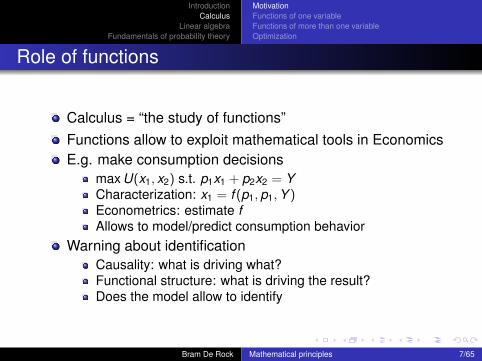
Role of functions

Calculus = “the study of functions”Functions allow to exploit mathematical tools in EconomicsE.g. make consumption decisions

max U(x1, x2) s.t. p1x1 + p2x2 = YCharacterization: x1 = f (p1,p1,Y )Econometrics: estimate fAllows to model/predict consumption behavior

Warning about identificationCausality: what is driving what?Functional structure: what is driving the result?Does the model allow to identify





Derivatives

Marginal changes are important in EconomicsThe impact of a infinitesimally small change of one of thevariablesComparative statistics: what is the impact of a pricechange?Optimization: what is the optimal consumption bundle?

Marginal changes are mostly studied by taking derivativesCharacterizing the impact depends on the function

f : D ⊆ Rn → Rk : (x1, . . . , xn) 7→ (y1, . . . yk ) = f (x1, . . . , xn)We will always take k = 1First look at n = 1 and then generalizeNote: N ⊂ Z ⊂ Q ⊂ R ⊂ C





Outline

1 Introduction


3 Linear algebra






Functions of one variable: f : D ⊆ R→ R

dfdx

= f ′ = lim∆x→0

f (x + ∆x)− f (x)

∆x

Limit of quotient of differencesIf it exists, then it is called the derivativef ′ is again a functionE.g. f (x) = 3x2 − 4E.g. discontinuous functions, border of domain, f (x) = |x |





Some important derivatives and rules

Let us abstract from specifying the domain D and assume thatc,n ∈ R0

If f (x) = c, then f ′(x) = 0If f (x) = cxn, then f ′(x) = ncxn−1

If f (x) = cex , then f ′(x) = cex

If f (x) = c ln(x), then f (x) = c 1x

(f (x)± g(x))′ = f ′(x)± g′(x)

(f (x)g(x))′ = f ′(x)g(x) + f (x)g′(x) 6= f ′(x)g′(x)

( f (x)g(x) )′ = f ′(x)g(x)−f (x)g′(x)

g(x)2





Application: the link with marginal changes

By definition it is the limit of changesSlope of the tangent line

Increasing or decreasing function (and thus impact)Does the inverse function exist?

First order approximation in some point cBased on expression for the tangent line in cf (c + ∆x) ≈ f (c) + f ′(c)(∆x)More general approximation: Taylor expansion





Application: elasticities

The elasticity of f in x : f ′(x)xf (x)

The limit of the quotient of changes in terms of percentagePercentage change of the function: f (x+∆x)−f (x)

f (x)

Percentage change of the variable: ∆xx

Quotient: f (x+∆x)−f (x)∆x

xf (x)

Is a unit independent informative numberE.g. the (price) elasticity of demand





Application: comparative statics for a simple marketmodel

Demand: Q = 10− 4PSupply: Q = 2 + αPP∗ = 8

4+α and Q∗ = 8+10α4+α

dP∗dα = −8

(4+α)2 and dQ∗dα = 32

(4+α)2

The elasticity of demand is −4P10−4P





Some exercises

Compute the derivative of the following functions (definedon R+)

f (x) = 17x2 + 5x + 7f (x) = −

√x + 3

f (x) = 1x2

f (x) = 17x2ex

f (x) = xln(x)x2−4

Let f (x) : R→ R : x 7→ x2 + 5x .Determine on which region f is increasingIs f invertible?Approximate f in 1 and derive an expression for theapproximation errorCompute the elasticity in 3 and 5





The chain rule

Often we have to combine functionsIf z = f (y) and y = g(x), then z = h(x) = f (g(x))

We have to be careful with the derivativeA small change in x causes a chain reaction

It changes y and this in turn changes z

That is why dzdx = dz

dydydx = f ′(y)g′(x)

Can easily be generalized to compositions of more than twofunctionsdzdx = dz

dydydu · · ·

dvdx

E.g. if h(x) = ex2, then h′(x) = ex2

2x





Higher order derivatives

The derivative is again a function of which we can takederivativesHigher order derivatives describe the changes of thechangesNotation

f ′′(x) or more generally f (n)(x)ddx ( df

dx ) or more generally dn

dxn f (x)

E.g. if f (x) = 5x3 + 2x , then f ′′′(x) = f (3)(x) = 30





Application: concave and convex functions

f : D ⊂ Rn → R

f is concave∀x , y ∈ D,∀λ ∈ [0,1] : f (λx + (1−λ)y) ≥ λf (x) + (1−λ)f (y)If n = 1, ∀x ∈ D : f ′′(x) ≤ 0

f is convex∀x , y ∈ D,∀λ ∈ [0,1] : f (λx + (1−λ)y) ≤ λf (x) + (1−λ)f (y)If n = 1, ∀x ∈ D : f ′′(x) ≥ 0





Application: concave and convex functions

Very popular and convenient assumptions in EconomicsE.g. optimization

Sometimes intuitive interpretationE.g. risk-neutral, -loving, -averse

Don’t be confused with a convex setS is a set⇔ ∀x , y ∈ S,∀λ ∈ [0,1] : λx + (1− λ)y ∈ S





Some exercises

Compute the first and second order derivative of thefollowing functions (defined on R+)

f (x) = −πf (x) = −

√5x + 3

f (x) = e−3x

f (x) = ln(5x)f (x) = x3 − 6x2 + 17

Determine which of these functions are concave or convex





Outline

1 Introduction


3 Linear algebra






Functions of more than one variable: f : D ⊆ Rn → R

Same applications in mind but now several variablesE.g. what is the marginal impact of changing x1, whilecontrolling for other variables?

Look at the partial impact: partial derivatives∂∂xi

f (x1, . . . , xn) = fxi =

lim∆xi→0f (x1,...,xi +∆xi ,...,xn)−f (x1,...,xi ,...,xn)

∆xiSame interpretation as before, but now fixing remainingvariables

E.g. f (x1, x2, x3) = 2x21 x2 − 5x3

∂∂x1

f (x1, x2, x3) = 4x1x2∂∂x2

f (x1, x2, x3) = 2x21

∂∂x3

f (x1, x2, x3) = −5





Partial derivative

Geometric interpretation: slope of tangent line in the xidirectionSame rules holdHigher order derivatives

∂2

∂x2if (x1, . . . , xn)

∂2

∂xi xjf (x1, . . . , xn) = ∂2

∂xj xif (x1, . . . , xn)

E.g. ∂2

∂x21f (x1, x2, x3) = 4x2 and ∂2

∂x1x3f (x1, x2, x3) = 0





Some remarks

Gradient: ∇f (x1, . . . , xn) = ( ∂f∂x1, . . . , ∂f

∂xn)

Chain rule: special casex1 = g1(t), . . . , xn = gn(t) and f (x1, . . . , xn)h(t) = f (x1, . . . , xn) = f (g1(t), . . . ,gn(t))dh(t)

dt = h′(t) = ∂f (x1,...,xn)∂x1

dx1dt + · · ·+ ∂f (x1,...,xn)

∂xn

dxndt

E.g. f (x1, x2) = x1x2, g1(t) = et and g2(t) = t2

h′(t) = et t2 + et2t





Some remarks

Slope of indifference curve of f (x1, x2)

Indifference curve: all (x1, x2) for which f (x1, x2) = C (withC some give number)Implicit function theorem: f (x1,g(x1)) = C∂∂x1

f (x1, x2) + ∂∂x2

f (x1, x2) dgdx1

= 0

Slope = −∂

∂x1f (x1,x2)

∂∂x2

f (x1,x2)





Some exercises

Compute the gradient and all second order partialderivatives for the following functions (defined on R+)

f (x1, x2) = x21 − 2x1x2 + 3x2

2f (x1, x2) = ln(x1x2)f (x1, x2, x3) = ex1+2x2 − 3x1x3

Compute the marginal rate of substitution for the utilityfunction U(x1, x2) = xα1 xβ2





Outline

1 Introduction


3 Linear algebra






Optimization: important use of derivatives

Many models in economics entail optimizing behaviorMaximize/Minimize objective subject to constraints

Characterize the points that solve these modelsNote on Mathematics vs Economics

Profit = Revenue - CostMarginal revenue = marginal costMarginal profit = zero





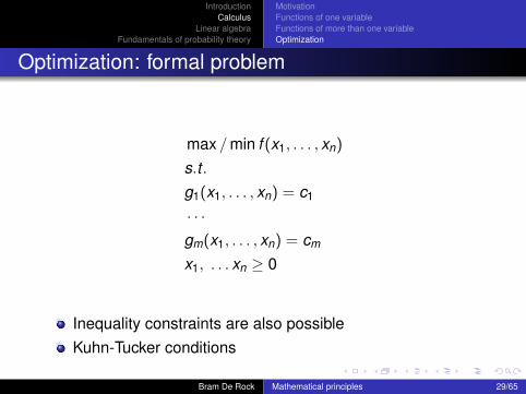
Optimization: formal problem

max /min f (x1, . . . , xn)

s.t .g1(x1, . . . , xn) = c1

· · ·gm(x1, . . . , xn) = cm

x1, . . . xn ≥ 0

Inequality constraints are also possibleKuhn-Tucker conditions





Necessity and sufficiency

Necessary conditions based on first order derivativesLocal candidate for an optimum

Sufficient conditions based on second order derivativesNecessary condition is sufficient if

The constraints are convex functionsE.g. no constraints, linear constraints, . . .The objective function is concave: global maximum isobtainedThe objective function is convex: global minimum isobtainedOften the “real” motivation in Economics





Necessary conditions

1 Free optimizationNo constraintsf ′(x∗) = 0 if n = 1∂∂xi

f (x∗1 , . . . , x∗n ) = 0 for i = 1, . . . ,n

Intuitive given our geometric interpretation






2 Optimization with positivity constraintsNo gi constraintsOn the boundary extra optima are possibleOften ignored: interior solutionsx∗i ≥ 0 for i = 1, . . . ,nx∗i

∂∂xi

f (x∗1 , . . . , x∗n ) = 0 for i = 1, . . . ,n

∂∂xi

f (x∗1 , . . . , x∗n ) ≤ 0 for all i = 1, . . . ,n simultaneously OR

∂∂xi

f (x∗1 , . . . , x∗n ) ≥ 0 for all i = 1, . . . ,n simultaneously






3 Constrained optimization without positivity constraintsDefine Lagrangian: L(x1, . . . , xn, λ1, . . . , λm) =f (x1, . . . , xn)− λ1(g1(x1, . . . , xn))− · · · − λm(gm(x1, . . . , xn))∂∂xi

L(x∗1 , . . . , x∗n , λ∗1, . . . , λ

∗m) = 0 for all i = 1, . . . ,n

∂∂λj

L(x∗1 , . . . , x∗n , λ∗1, . . . , λ

∗m) = 0 for all j = 1, . . . ,m

Alternatively: ∇f (x∗1 , . . . , x∗n ) =

λ∗1∇g1(x∗1 , . . . , x∗n ) + · · ·+ λ∗m∇gm(x∗1 , . . . , x

∗n )

Some intuition: geometric interpretationLagrange multiplier = shadow price





Application: utility maximization

max U(x1, x2) = xα1 x1−α2 s.t . p1x1 + p2x2 = Y

L(x1, x2, λ1) = xα1 x1−α2 − λ1(p1x1 + p2x2 − Y )

∂L∂x1

= αxα−11 x1−α

2 − λ1p1 = 0∂L∂x2

= (1− α)xα1 x−α2 − λ1p2 = 0∂L∂λ1

= p1x1 + p2x2 − Y = 0

x∗1 = αYp1, x∗2 = (1−α)Y

p2and λ∗1 = ( αp1

)α( (1−α)p2

)(1−α)





Some exercises

Find the optima for the following problemsmax /min x3 − 12x2 + 36x + 8max /min x3

1 − x32 + 9x1x2

min 2x21 + x1x2 + 4x2

2 + x1x3 + x23 − 15x1

max x1x2 s.t. x1 + 4x2 = 16max yz + xz s.t. y2 + z2 = 1 and xz = 3

Add positivity constraints to the above unconstrainedproblems and do the same




MotivationMatrix algebraThe link with vector spacesApplication: solving a system of linear equations

Outline

1 Introduction

2 Calculus

3 Linear algebraMotivationMatrix algebraThe link with vector spacesApplication: solving a system of linear equations






Motivation

Matrices allow to formalize notationUseful in solving system of linear equationsUseful in deriving estimators in econometricsAllows us to make the link with vector spaces





Outline

1 Introduction

2 Calculus







Matrices

A = (aij)i=1,...,n;j=1,...,m =

a11 a12 · · · a1ma21 a22 · · · a2m

...... · · ·

...an1 an2 · · · anm

aij ∈ R and A ∈ Rn×m

n rows and m columns

Square matrix if n = mNotable square matrices

Symmetric matrix: aij = aji for all i , j = 1, . . . ,nDiagonal matrix: aij = 0 for all i , j = 1, . . . ,n and i 6= jTriangular matrix: only non-zero elements above (or below)the diagonal





Matrix manipulations

Let A,B ∈ Rn×m and k ∈ REquality: A = B ⇔ aij = bij for all i , j = 1, . . . ,nScalar multiplication: kA = (kaij)i=1,...,n;j=1,...,m

Addition: A± B = (aij ± bij)i=1,...,n;j=1,...,mDimensions must be equal

Transposition: A′ = At = (aji)j=1,...,m;i=1,...,nA ∈ Rn×m and At ∈ Rm×n

(A± B)t = At ± Bt

(kA)t = kAt

(At )t = A





Matrix multiplication

Let A ∈ Rn×m and B ∈ Rm×k

AB = (∑m

h=1 aihbhj)i=1,...,n;j=1,...,k

Multiply the row vector of A with the column vector of BAside: scalar/inner product and norm of vectorsOrthogonal vectors

Number of columns of A must be equal to number of rowsof BAB 6= BA, even if both are square matrices(AB)t = BtAt





Example

Let A =

(2 11 1

),B =

(1 −10 2

)and C =

(1 2 33 2 1

)

At =

(2 11 1

),Bt

(1 0−1 2

)and C =

1 32 23 1

AB =

(2 01 1

)and BA =

(1 02 2

)AC =

(5 6 74 4 4

)(AB)t = BtAt =

(2 10 1

)





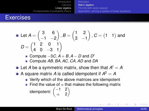
Exercises

Let A =

(3 6−1 −2

),B =

(1 23 −1

),C =

(1 1

)and

D =

(1 2 0 14 0 −3 1

)Compute −3C,A + B,A− D and Dt

Compute AB,BA,AC,CA,AD and DA

Let A be a symmetric matrix, show then that At = AA square matrix A is called idempotent if A2 = A

Verify which of the above matrices are idempotentFind the value of α that makes the following matrix

idempotent:(−1 2α 2

)





Two numbers associated to square matrices: trace

Let A,B,C ∈ Rn×n

Trace(A) = tr(A) =∑n

i=1 aii

Used in econometricsProperties

tr(At ) = tr(A)tr(A + B) = tr(A) + tr(B)tr(cA) = ctr(A) for any c ∈ Rtr(AB) = tr(BA)tr(ABC) = tr(BCA) = tr(CAB) 6= tr(ACB)(= tr(BAC) =tr(CBA))





Two numbers associated to square matrices: trace

Example

Let A =

(3 6−1 −2

)and B =

(1 23 −1

)Then AB =

(21 0−7 0

), BA =

(1 210 20

)and

A + B =

(4 82 −3

)tr(A) = 1, tr(B) = 0 and tr(A + B) = 1tr(AB) = 21 = tr(BA)





Two numbers associated to square matrices:determinant

Let A ∈ Rn×n

If n = 1, then det(A) = a11

If n = 2, thendet(A) = a11a22 − a12a21 = a11 det(a22)− a12 det(a21)

If n = 3, then det(A) = a11 det(

a22 a23a32 a33

)−

a12 det(

a21 a23a31 a33

)+ a13 det

(a21 a22a31 a32

)Can be generalized to any nWorks with columns too






Let A,B ∈ Rn×n

det(At ) = det(A)

det(A + B) 6= det(A) + det(B)

det(cA) = c det(A) for any c ∈ Rdet(AB) = det(BA)

A is non-singular (or regular) if A−1 existsI.e. AA−1 = A−1A = InIn is a diagonal matrix with 1 on the diagonalDoes not always existdet(A) 6= 0






Example

Let A =

(3 6−1 −2

)and B =

(1 23 −1

)Then AB =

(21 0−7 0

), BA =

(1 210 20

)and

A + B =

(4 82 −3

)det(A) = 0, det(B) = −7 and det(A + B) = −28det(AB) = 0 = det(BA)





Exercises

Let A =

2 4 50 3 01 0 1

Compute tr(A) and det(−2A)

Show that for any triangular matrix A, we have that det(A)is equal to the product of the elements on the diagonalLet A,B ∈ Rn×n and assume that B is non-singular

Show that tr(B−1AB) = tr(A)Show that tr(B(BtB)−1Bt ) = n

Let A,B ∈ Rn×n be two non-singular matricesShow that AB is then also invertibleGive an expression for (AB)−1





Outline

1 Introduction

2 Calculus







A notion of vector spaces

A set of vectors V is a vector space ifAddition of vectors is well-defined∀a,b ∈ V : a + b ∈ VScalar multiplication is well-defined∀k ∈ R,∀a ∈ V : ka ∈ V

We can take linear combinations∀k1, k2 ∈ R,∀a,b ∈ V : k1a + k2b ∈ V

E.g. R2 or more generally Rn

Counterexample R2+





Linear (in)dependence

Let V be a vector spaceA set of vectors v1, . . . , vn ∈ V is linear dependent if one ofthe vectors can be written as a linear combination of theothers

∃k1, . . . kn−1 ∈ R : vn = k1v1 + · · ·+ kn−1vn−1

A set of vectors are linear independent if they are not lineardependent

∀k1, . . . kn ∈ R : k1v1 + · · ·+ knvn = 0⇒ k1 = · · · = kn = 0

In a vector space of dimension n, the number of linearindependent vectors cannot be higher than n





Linear (in)dependence

ExampleR2 is a vector space of dimension 2v1 = (1,0), v2 = (1,2), v3 = (−1,4) and v4 = (2,4)

v3 = −3v1 + 2v2, so v1, v2, v3 are linear dependentv4 = 2v2, so v2, v4 are linear dependentv1, v2 are linear independentv3 is linear independent





Link with matrices: rank

Let A ∈ Rn×m and B ∈ Rm×k

The row rank of A is the maximal number of linearindependent rows of AThe column rank of A is the maximal number of linearindependent columns of ARank of A = column rank of A = row rank of AProperties

rank(A) ≤ min(n,m)rank(AB) ≤ min(rank(A), rank(B))rank(A) = rank(AtA) = rank(AAt )If n = m, then A has maximal rank if and only if det(A) 6= 0





Link with matrices: rank

Example

Let A =

(3 6−1 −2

)and B =

(1 23 −1

)Then AB =

(21 0−7 0

), BA =

(1 210 20

)rank(A) = 1 and rank(B) = 2rank(AB) = 1





Exercises

Let A =

2 4 50 3 01 0 1

Show in two ways that A has maximal rank

Let A,B ∈ Rn×m

Show that there need not be any relation betweenrank(A + B), rank(A) and rank(B)

Show that if A is invertible, then it needs to have a maximalrank





Outline

1 Introduction

2 Calculus







System of linear equations

Linear equations in the unknowns x1, . . . , xmNot x1x2, x2

m,...Constraints hold with equality

Not 2x1 + 5x2 ≤ 3

E.g.{

2x1 + 3x2 − x3 = 5−x1 + 4x2 + x3 = 0





Using matrix notation

m unknowns: x1, . . . , xm

n linear constraints: ai1x1 + · · ·+ aimxm = bi withai1, . . .aim,bi ∈ R and i = 1, . . . ,nAx = b

A = (aij )i=1,...,n,j=1,...,mx = (xi )i=1,...,nb = (bi )i=1,...,n

Homogeneous if bi = 0 for all i = 1, . . . ,n





Solving these system

Solve this by logical reasoningEliminate or substitute variablesCan also be used for non-linear systems of equationsCan be cumbersome for larger systems

Use matrix notationGaussian elimination of the augmented matrix (A|b)Can be programmedOnly for systems of linear equationsTheoretical statements are possible





Example

{−x1 + 4x2 = 02x1 + 3x2 = 5

x1 = 4x2 ⇒ 11x2 = 5⇒ x2 = 511 and x1 = 20

11(−1 42 3

)(x1x2

)=

(05

)Take linear combinations of rows of the augmented matrix

Is the same as taking linear combinations of the equations(−1 4 |02 3 |5

)⇒(−1 4 | 00 11 | 5

)⇒(−1 0 | −20

110 11 | 5

)





Theoretical results

Consider the linear system Ax = b with A ∈ Rn×m

This system has a solution if and only ifrank(A) = rank(A|b)

rank(A) ≤ rank(A|b) by definitionIs the (column) vector b a linear combination of the columnvectors of A?If rank(A) < rank(A|B), the answer is noIf rank(A) = rank(A|B), the answer is yes

The solution is unique if rank(A) = rank(A|B) = mn ≥ m

There are∞ many solutions if rank(A) = rank(A|B) < mn < m or too many constraints are ‘redundant’





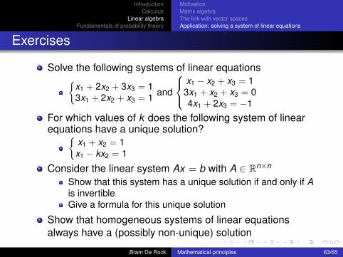
Exercises

Solve the following systems of linear equations{x1 + 2x2 + 3x3 = 13x1 + 2x2 + x3 = 1 and

x1 − x2 + x3 = 13x1 + x2 + x3 = 04x1 + 2x3 = −1

For which values of k does the following system of linearequations have a unique solution?{

x1 + x2 = 1x1 − kx2 = 1

Consider the linear system Ax = b with A ∈ Rn×n

Show that this system has a unique solution if and only if Ais invertibleGive a formula for this unique solution

Show that homogeneous systems of linear equationsalways have a (possibly non-unique) solution




Outline

1 Introduction

2 Calculus

3 Linear algebra





To be continued


principles in economics and mathematics: the mathematical … · introduction calculus linear...

Documents