lecture notes for chapter 11 - bcit school of...
TRANSCRIPT

Lecture Notes for Chapter 11
Kevin Wainwright
April 26, 2014
1 Optimization withMore than One Vari-able
Suppose we want to maximize the following function
z = f(x, y) = 10x+ 10y + xy − x2 − y2
Note that there are two unknowns that must be solved for: x andy. This function is an example of a three-dimensional dome. (i.e. theroof of BC Place)To solve this maximization problem we use partial derivatives.
We take a partial derivative for each of the unknown choice variablesand set them equal to zero
∂z∂x = fx = 10 + y − 2x = 0 The slope in the ”x”direction = 0∂z∂y = fy = 10 + x− 2y = 0 The slope in the ”y”direction = 0
This gives us a set of equations, one equation for each of the un-known variables. When you have the same number of independentequations as unknowns, you can solve for each of the unknowns.rewrite each equation as
1

y = 2x− 10
x = 2y − 10
substitute one into the other
x = 2(2x− 10)− 10
x = 4x− 30
3x = 30
x = 10
similarly,y = 10
REMEMBER: To maximize (minimize) a function of manyvariables you use the technique of partial differentiation. This producesa set of equations, one equation for each of the unknowns. You thensolve the set of equations simulaneously to derive solutions for each ofthe unknowns.
1.0.1 Second order Conditions (second derivative Test)
To test for a maximum or minimum we need to check the second partialderivatives. Since we have two first partial derivative equations (fx,fy)and two variable in each equation, we will get four second partials( fxx, fyy, fxy, fyx)Using our original first order equations and taking the partial deriv-
atives for each of them (a second time) yields:
2
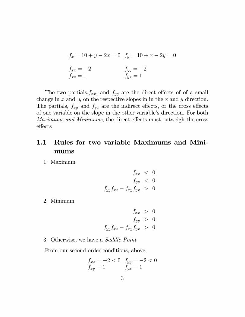
fx = 10 + y − 2x = 0 fy = 10 + x− 2y = 0
fxx = −2 fyy = −2fxy = 1 fyx = 1
The two partials,fxx, and fyy are the direct effects of of a smallchange in x and y on the respective slopes in in the x and y direction.The partials, fxy and fyx are the indirect effects, or the cross effectsof one variable on the slope in the other variable’s direction. For bothMaximums and Minimums, the direct effects must outweigh the crosseffects
1.1 Rules for two variable Maximums and Mini-mums
1. Maximum
fxx < 0
fyy < 0
fyyfxx − fxyfyx > 0
2. Minimum
fxx > 0
fyy > 0
fyyfxx − fxyfyx > 0
3. Otherwise, we have a Saddle Point
From our second order conditions, above,
fxx = −2 < 0 fyy = −2 < 0fxy = 1 fyx = 1
3

andfyyfxx − fxyfyx = (−2)(−2)− (1)(1) = 3 > 0
therefore we have a maximum.
1.2 Using Differentials Approach
Givenz = f(x, y)
Thendz = fxdx+ fydy
ifdx 6= 0, dy 6= 0
anddz = 0 (critical point)
Then it must be true that
fx = fy = 0 or ∂z∂x = ∂z
∂y = 0
Fx = 0: Means z is not changing in the x-directionFy = 0: Means z is not changing in the y-directionThis is the First Order Necessary Condition for a max or min
1.3 Second Order Conditions
Givenz = f(x, y)
The first derivative (differential) is
dz = fxdx+ fydy
4

Take the total differential a second time, treating dx and dy as constants
d2z = fxxdxdx+ fyydydy + fxydxdy + fyxdydx
= fxxdx2 + fyydy
2 + fxydxdy + fyxdydx
where
fxx = 2nd partial derivative with respect to xfyy = 2nd partial derivative with respect to y
fxy = Change in(∂z∂x
)from a ∆ in y
fyx = Change in(∂z∂y
)from a ∆ in x︸ ︷︷ ︸
fxy,fyx are cross partial derivatives
1.4 Example: Two Market Monopoly with JointCosts
A monopolist offers two different products, each having the followingmarket demand functions
q1 = 14− 14p1
q2 = 24− 12p2
The monopolist’s joint cost function is
C(q1, q2) = q21 + 5q1q2 + q22
The monopolist’s profit function can be written as
π = p1q1 + p2q2 − C(q1, q2) = p1q1 + p2q2 − q21 − 5q1q2 − q22
which is the function of four variables: p1, p2, q1,and q2. Usingthe market demand functions, we can eliminate p1and p2 leaving us
5

with a two variable maximization problem. First, rewrite the demandfunctions to get the inverse functions
p1 = 56− 4q1p2 = 48− 2q2
Substitute the inverse functions into the profit function
π = (56− 4q1)q1 + (48− 2q2)q2 − q21 − 5q1q2 − q22
The first order conditions for profit maximization are
∂π∂q1
= 56− 10q1 − 5q2 = 0∂π∂q2
= 48− 6q2 − 5q1 = 0
Solve the first order conditions using Cramer’s rule. First, rewritein matrix form [
10 55 6
] [q1q2
]=
[5648
]where |A| = 35
q∗1 =
∣∣∣∣ 56 548 6
∣∣∣∣35
= 2.75
q∗2 =
∣∣∣∣ 10 565 48
∣∣∣∣35
= 5.7
Using the inverse demand functions to find the respective prices,we get
p∗1 = 56− 4(2.75) = 45p∗2 = 48− 2(5.7) = 36.6
6

From the profit function, the maximum profit is
π = 213.94
Next, check the second order conditions to verify that the profitis at a maximum. The various second derivatives can be set up in amatrix called a Hessian The Hessian for this problem is
H =
[π11 π12π21 π22
]=
[−10 −5−5 −6
]The suffi cient conditions are
|H1| = π11 = −10 < 0 (First Principle Minor of Hessian)|H2| = π11π22 − π12π21 = (−10)(−6)− (−5)2 = 35 > 0 (determinant)
Therefore the function is at a maximum. Further, since the signsof |H1| and |H2| are invariant to the values of q1and q2, we know thatthe profit function is strictly concave.
1.5 Example: Profit Max Capital and Labour
Suppose we have the following production function
q = Outputq = f(K,L) = L
12 +K
12 L = Labour
K = Capital
Then the profit function for a competitive firm is
π = Pq − wL− rK P = Market Priceor w = Wage Rateπ = PL
12 + PK
12 − wL− rK r = Rental Rate
7

First order conditions
General Form1. ∂π
∂L = P2L
−12 − w = 0 PfL − w = 0
2. ∂π∂k = P
2K−12 − r = 0 PfK − r = 0
Solving (1) and (2), we get
L∗ = (2wP )−2 K∗ = (2rP )−2
Second order conditions (Hessian)
πLL = PfLL = −P4 L
−32 < 0
πKK = PfKK = −P4 K
−32 < 0
πLK = πKL = PfLK = PfKL = 0
or, in matrix form
H =
∣∣∣∣ πLL πLKπKL πKK
∣∣∣∣ =
∣∣∣∣ −P4 L−32 0
0 −P4 K
−32
∣∣∣∣P[fLLfKK − (fLK)2
]=
(−P4L
−32
)(−P4K
−32
)− 0 > 0
Differentiate first order of conditions with respect to capital (K)and labour (L)
=⇒Therefore profit maximization
Example: If P = 1000, w = 20, and r = 10
1. Find the optimal K, L, and π
2. Check second order conditions
8

1.6 Example: Cobb-Douglas production functionand a competitive firm
Consider a competitive firm with the following profit function
π = TR− TC = PQ− wL− rK
where P is price, Q is output, L is labour and K is capital, andw and r are the input prices for L and K respectively. Since the firmoperates in a competitive market, the exogenous variables are P,w andr. There are three endogenous variables, K, L and Q. However output,Q, is in turn a function of K and L via the production function
Q = f(K,L)
which in this case, is the Cobb-Douglas function
Q = LaKb
where a and b are positive parameters. If we further assume de-creasing returns to scale, then a + b < 1. For simplicity, let’s considerthe symmetric case where a = b = 1
4
Q = L14K
14
Substituting Equation 3 into Equation 1 gives us
π(K,L) = PL14K
14 − wL− rK
The first order conditions are
∂π∂L = P
(14
)L−
34K
14 − w = 0
∂π∂K = P
(14
)L
14K−
34 − r = 0
9

This system of equations define the optimal L and K for profitmaximization. But first, we need to check the second order conditionsto verify that we have a maximum.The Hessian for this problem is
H =
[πLL πLKπKL πKK
]=
[P (− 3
16)L− 74K
14 P
(14
)2L−
34K−
34
P(14
)2L−
34K−
34 P
(− 316
)L
14K
74
]
The suffi cient conditions for a maximum are that |H1| < 0 and|H| > 0. Therefore, the second order conditions are satisfied.We can now return to the first order conditions to solve for the
optimal K and L. Rewriting the first equation in Equation 5 to isolateK
P(14
)L−
34K
14 = w
K = (4wp L34 )4
Substituting into the second equation of Equation 5
P4L
14K−
34 =
(P4
)L
14
[(4wp L
34
)4]− 34= r
= P 4(14
)4w−3L−2 = r
Re-arranging to get L by itself gives us
L∗ = (P
4w−
34r−
14 )2
Taking advantage of the symmetry of the model, we can quicklyfind the optimal K
K∗ = (P
4r−
34w−
14 )2
L∗ and K∗ are the firm’s factor demand equations.
10

1.7 Young’s Theorem
For cross partial "effects" the order of differentiation is immaterial.Therefore:
fxy = fyx
As long as the cross partials are continuous.
In the case of GENERAL FUNCTIONS , this will always be as-sumed to be true!
1.7.1 Example:z = x3 + 5xy = y2
fx = 3x2 + 5y fy = 5x− 2y
fxx = 6x fyy = −2fxy = 5 fyx = 5︸ ︷︷ ︸
fxy=fyx
1.8 Quadratic Form
The functionq = ax2 + 2bxy + cy2
is a quadratic form. A quadratic can be written in matrix form as:
q1x1
=[x y
]1x2
[a bc d
]2x2
[xy
]2x1
Det = (ac− b2)
11
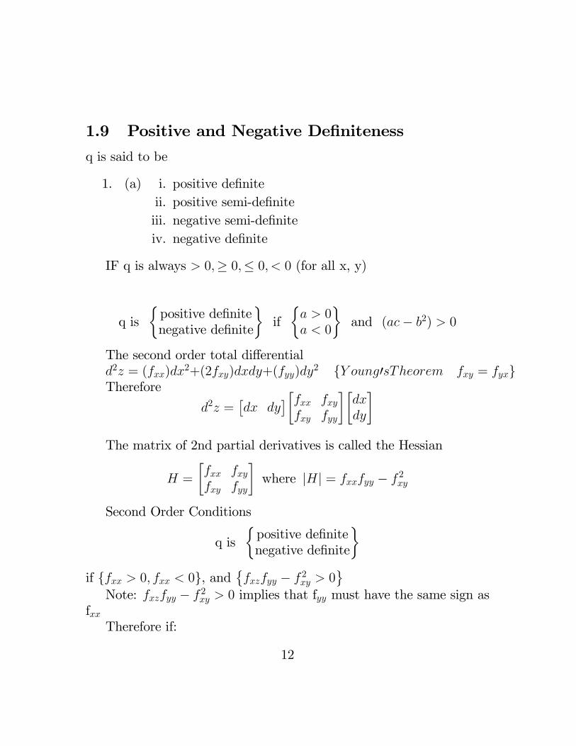
1.9 Positive and Negative Definiteness
q is said to be
1. (a) i. positive definiteii. positive semi-definiteiii. negative semi-definiteiv. negative definite
IF q is always > 0,≥ 0,≤ 0, < 0 (for all x, y)
q is{positive definitenegative definite
}if{a > 0a < 0
}and (ac− b2) > 0
The second order total differentiald2z = (fxx)dx
2+(2fxy)dxdy+(fyy)dy2 {Y oung′sTheorem fxy = fyx}
Therefore
d2z =[dx dy
][fxx fxyfxy fyy
][dxdy
]The matrix of 2nd partial derivatives is called the Hessian
H =
[fxx fxyfxy fyy
]where |H| = fxxfyy − f 2xy
Second Order Conditions
q is{positive definitenegative definite
}if {fxx > 0, fxx < 0}, and
{fxzfyy − f 2xy > 0
}Note: fxzfyy − f 2xy > 0 implies that fyy must have the same sign as
fxxTherefore if:
12

1. fx = fy = 0 (FOC), and if:
2. SOC
d2z is{negative definitepositive definite
}then z is
{a maximuma minimum
1.10 n-Variable Case
Givenz = f(x1, x2, ...xn)
For an Extremum (max or min):
f1 = f2 = f3 = ... = fn = 0 (First Order Conditions)
Then d2z in Matrix Form is
[dx1 dx2 ... dxn
](1xn)
f11 f12 f13 ... f1nf21 f22 ... ... f2nf31 f33 ... ...... ... ... ... ...fn1 ... ... ... fnn
(nxn)
dx1dx2dx3...dxn
(nx1)
For a Max: (Principal minors alternate signs)|H1| = f11 < 0, |H2| = f11f22 − f 212 > 0, |H3| < 0, ...(−1)n |Hn| > 0For a Min: (Principal minors have the same sign)|H1| > 0, |H2| > 0, ... |Hn| > 0
13

1.10.1 Example: Output Maximization
LetQ = 10L+ 10K + LK − L2 −K2
F.O.C.’s[∂Q∂L = 10 +K − 2L = 0∂Q∂K = 10 + L− 2K = 0
]OR
{2L−K = 10−L+ 2K = 10
}2 Equations with 2 unknowns from FOC. Matrix Form:[
2 −1−1 2
] [LK
]=
[1010
] {Det = 3
}Cramer’s Rule
L =
∣∣∣∣10 −110 2
∣∣∣∣3
=20 + 10
3= 10
K =
∣∣∣∣ 2 10−1 10
∣∣∣∣3
=20 + 10
3= 10
Now check 2nd order conditions from F.O.C
10 +K − 2L = 010 + L− 2K = 0
}when K,L=10 FOC’s
are identities
S.O.C.
dK − 2dL = 0dL− 2dK = 0
14

Find the Hessian [−2 11 −2
] [dLdK
]=
[00
]
H =
[QLL QLK
QKL QKK
]=
[−2 11 −2
]
QLL = −2 < 0 QLLQKK −Q2KL = (−2)(−2)− (1) > 0︸ ︷︷ ︸Therefore Q is Max at K=10, L=10
1.11 Economic Interpretation of the 2nd OrderConditions
Given the production function
Q = Q(K,L)
QL > 0, QLL < 0 implies the "Law of Diminishing Returns"
The conditionQLLQKK −Q2KL > 0
1. (a) says that for a Maximum the direct effects (QLL,QKK) mustoutweigh the indirect effects (QKLQLK)
(b) a production function can have the properties of "the lawof diminishing returns" and "increasing returns to scale"at the same time
(c) Therefore Q(K,L) has no unconstrained maximum
15

1.12 Profit Maximization and Comparative Stat-ics
Let q = f(x1, x2)be the production function.The profit function is
π = pf(x1, x2)− w1x1 − w2x2
where p = output price, w1,w2 = factor prices of x1 and x2 respectivelyThe FOC‘s for profit max
∂π∂x1
= pf1 − w1 = 0∂π2∂x2
= pf2 − w2 = 0
}This gives us 2 equations and
2 unknowns, x∗1,x∗2
16

Solving the F.O.C’s we get:
x∗1 = x∗1(w1, w2, P ) x∗2 = x∗2(w1, w2, P ){x∗1,x∗2 as functions of exogenous variables}
2nd order conditionsFrom the F.O.C.’s
pf1 − w1 = 0pf2 − w2 = 0
}at x1=x∗1, x2=x
∗2
Differentiate again for the Hessian[pf11 pf12pf21 pf22
](dx1dx2
)=
(00
)H =
[pf11 pf12pf21 pf22
]= p
[f11 f12f21 f22
]For Maximum
|H1| = f11 < 0 |H2| = f11f22 − f 212 > 0
1.13 Comparative Statics
By substituting
x∗1 = x∗1(w1, w2, P ) x∗2 = x∗2(w1, w2, P )
back into the F.O.C.’s
Pf1 = (x∗1(w1, w2, P ), x∗2(w1, w2, P ))− w1 = 0
Pf2 = (x∗1(w1, w2, P ), x∗2(w1, w2, P ))− w2 = 0
The F.O.C.‘s become identities that implicitly define x1,x2 as functionsof w1,w2,and P. Therefore to find
∂x∗1∂w1
, ∂x∗2
∂w1etc. we can use the implicit
function theorem by finding the Jacobian of the F.O.C.’s
17

Find: ∂x∗1∂w1
, ∂x∗2
∂w1Totally differentiate with respect to w1
Pf11∂x∗1∂w1
+ Pf12∂x∗2∂w1− dw1dw1
= 0
{dw1dw1
= 1
}Pf21
∂x∗1∂w1
+ Pf22∂x∗2∂w1
= 0
Matrix Form: [Pf11 Pf12Pf21 Pf22
]( ∂x∗1∂w1∂x∗2∂w1
)=
(10
)The Jacobian determinant
|J | = P (f11f22 − f 212) > 0
The Jacobian of the F.O.C.’s is also the Hessian of the S.O.C.’s
1.13.1 Solving by Cramer’s Rule
∂x∗1∂w1
=
∣∣∣∣1 Pf120 Pf22
∣∣∣∣|H| =
Pf22P (f11f22 − f 212)
=f22
f11f22 − f 212< 0
∂x∗2∂w1
=
∣∣∣∣Pf11 1Pf21 0
∣∣∣∣|H| ==
−f22f11f22 − f 212
≷ 0?
∂x∗1∂w1
< 0 implies downward sloping factor demand curve. For ∂x∗2∂w1
thissign depends on the relationship in production between x1 and x2
18
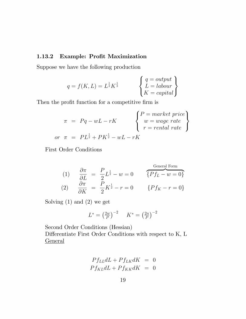
1.13.2 Example: Profit Maximization
Suppose we have the following production
q = f(K,L) = L12K
12
q = outputL = labourK = capital
Then the profit function for a competitive firm is
π = Pq − wL− rK
P = market pricew = wage rater = rental rate
or π = PL
12 + PK
12 − wL− rK
First Order Conditions
(1)∂π
∂L=
P
2L
12 − w = 0
General Form︷ ︸︸ ︷{PfL − w = 0}
(2)∂π
∂K=
P
2K
12 − r = 0 {PfK − r = 0}
Solving (1) and (2) we get
L∗ =(2wP
)−2K∗ =
(2nP
)−2Second Order Conditions (Hessian)Differentiate First Order Conditions with respect to K, LGeneral
PfLLdL+ PfLKdK = 0
PfKLdL+ PfKKdK = 0
19

Hessian (PfLL PfLKPfKL PfKK
)(dLdK
)|H1| = PfLL < 0
|H2| = P[fLLfKK − (fKK)2
]> 0
Specific
−P4L
−32 dL+ (0)dK = 0
−P4K
−32 dL+ (0)dL = 0
Hessian (−P4L
−32 0
0 −P4K
−32
)(dLdK
)H1 = −P
4L
−32
|H2| =
(−P
4L
−32
)(−P
4K
−32
)− 0 > 0
|H2| for both general and specific >0, therefore Profit MaxFrom the FOC’s we know:
L∗ =(2wP
)−2K∗ =
(2rP
)−2by subbing K∗ and L∗ into the profit function, we get:
π∗ = PL12 + PK
12 − wL− rK
π∗ = P
[(2w
P
)−2] 12
+ P
[(2r
P
)−2] 12
− w(
2w
P
)−2− r
(2r
P
)−2π∗ =
P 2
2w+P 2
2r− P 2
4w− P 2
4r
20
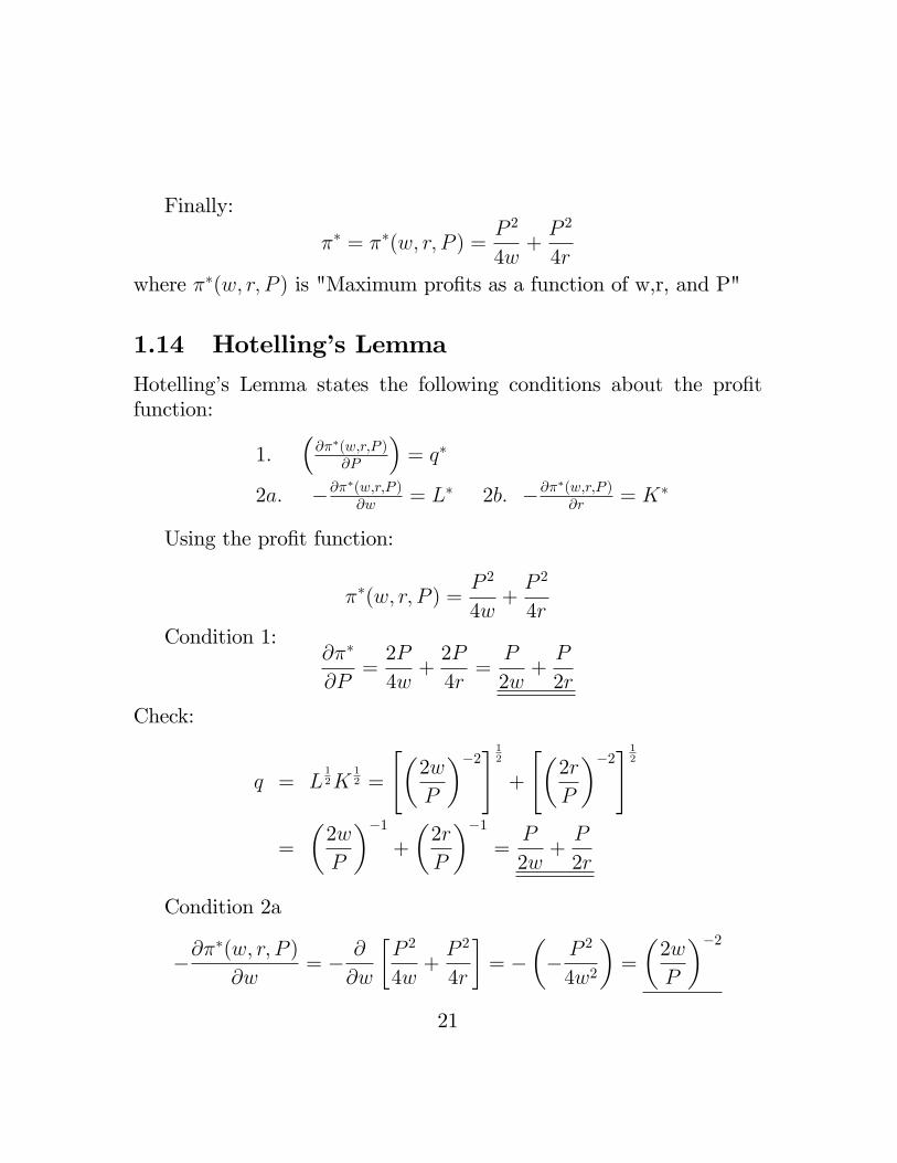
Finally:
π∗ = π∗(w, r, P ) =P 2
4w+P 2
4r
where π∗(w, r, P ) is "Maximum profits as a function of w,r, and P"
1.14 Hotelling’s Lemma
Hotelling’s Lemma states the following conditions about the profitfunction:
1.(∂π∗(w,r,P )
∂P
)= q∗
2a. −∂π∗(w,r,P )∂w = L∗ 2b. −∂π∗(w,r,P )
∂r = K∗
Using the profit function:
π∗(w, r, P ) =P 2
4w+P 2
4rCondition 1:
∂π∗
∂P=
2P
4w+
2P
4r=
P
2w+P
2r
Check:
q = L12K
12 =
[(2w
P
)−2] 12
+
[(2r
P
)−2] 12
=
(2w
P
)−1+
(2r
P
)−1=
P
2w+P
2r
Condition 2a
−∂π∗(w, r, P )
∂w= − ∂
∂w
[P 2
4w+P 2
4r
]= −
(− P 2
4w2
)=
(2w
P
)−221

Therefore −∂π∗
∂w = L∗
Condition 2b
−∂π∗(w, r, P )
∂r= −
(−P
2
4r2
)=
(2r
P
)−2= K∗
1.14.1 Factor Demand Curves
L∗ and K∗ are the firms demand curves for labour and capital
L∗ =P 2
4w2=⇒ ∂h∗
∂w= − P 2
4w3< 0
K∗ =P 2
4r2=⇒ ∂K∗
∂r− P 2
4r3< 0
Therefore: Downward sloping factor demand curves
1.15 Iso-Profit Curves (Level Curves)
Take the total differential of π∗(w, r, P ); let dπ∗ = 0
dπ∗ = − P 2
4w2dw +−P
2
4r2dr = 0
dr
dw= −
P 2
4w2
P 2
4r2
= − r2
w2< 0 (slope of Iso-Profit Curve)
Concave or Convex?
d
dw
(dr
dw
)= −
(−2
r2
w3
)= 2
r2
w3> 0
22

Therefore the slope of the Iso-Profit curve is negative(drdw
)but the
slope is becoming less negative:(d2rdw2
)> 0 Therefore: Convex
23
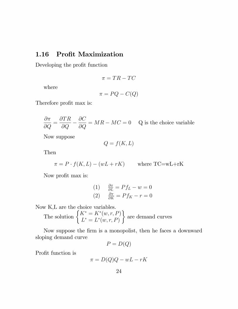
1.16 Profit Maximization
Developing the profit function
π = TR− TCwhere
π = PQ− C(Q)
Therefore profit max is:
∂π
∂Q=∂TR
∂Q− ∂C
∂Q= MR−MC = 0 Q is the choice variable
Now supposeQ = f(K,L)
Then
π = P · f(K,L)− (wL+ rK) where TC=wL+rK
Now profit max is:
(1) ∂π∂L = PfL − w = 0
(2) ∂π∂K = PfK − r = 0
Now K,L are the choice variables.
The solution{K∗ = K∗(w, r, P )L∗ = L∗(w, r, P )
}are demand curves
Now suppose the firm is a monopolist, then he faces a downwardsloping demand curve
P = D(Q)
Profit function isπ = D(Q)Q− wL− rK
24
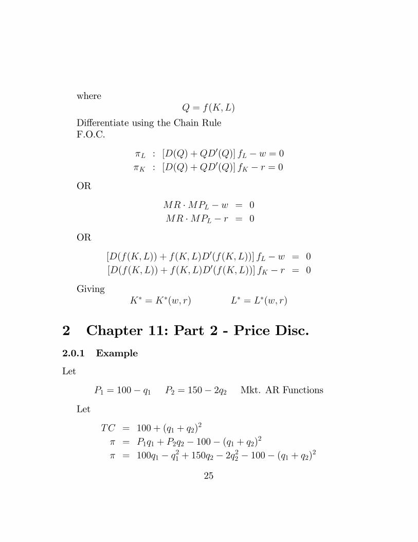
whereQ = f(K,L)
Differentiate using the Chain RuleF.O.C.
πL : [D(Q) +QD′(Q)] fL − w = 0
πK : [D(Q) +QD′(Q)] fK − r = 0
OR
MR ·MPL − w = 0
MR ·MPL − r = 0
OR
[D(f(K,L)) + f(K,L)D′(f(K,L))] fL − w = 0
[D(f(K,L)) + f(K,L)D′(f(K,L))] fK − r = 0
GivingK∗ = K∗(w, r) L∗ = L∗(w, r)
2 Chapter 11: Part 2 - Price Disc.2.0.1 Example
Let
P1 = 100− q1 P2 = 150− 2q2 Mkt. AR Functions
Let
TC = 100 + (q1 + q2)2
π = P1q1 + P2q2 − 100− (q1 + q2)2
π = 100q1 − q21 + 150q2 − 2q22 − 100− (q1 + q2)2
25
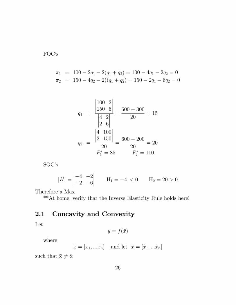
FOC‘s
π1 = 100− 2q1 − 2(q1 + q2) = 100− 4q1 − 2q2 = 0
π2 = 150− 4q2 − 2((q1 + q2) = 150− 2q1 − 6q2 = 0
q1 =
∣∣∣∣100 2150 6
∣∣∣∣∣∣∣∣4 22 6
∣∣∣∣ =600− 300
20= 15
q2 =
∣∣∣∣4 1002 150
∣∣∣∣20
=600− 200
20= 20
P ∗1 = 85 P ∗2 = 110
SOC’s
|H| =∣∣∣∣−4 −2−2 −6
∣∣∣∣ H1 = −4 < 0 H2 = 20 > 0
Therefore a Max**At home, verify that the Inverse Elasticity Rule holds here!
2.1 Concavity and Convexity
Lety = f(x̄)
wherex̄ = [x̄1, ...x̄n] and let x̂ = [x̂1, ...x̂n]
such that x̄ 6= x̂
26

Definition 1:y=f(x̄) is a concave function if
f (k · x̄+ (1− k) · x̂)︸ ︷︷ ︸Point on Dome
≥ kf(x̄) + (1− k)f(x̂)︸ ︷︷ ︸Line Segment
Definition 2:y=f(x̄) is convex if
f(kx̄+ (1− k)x̂) ≤ kf(x̄) + (1− k)f(x̂)
for strict concavity/convexity replace the weak inequalities with strictinequalities.
If the function y=f(x̄) is twice differentiable, then the followingholds:
Theorem 1: y=f(x̄) is concave/convex if and only the Hessian, |H|is negative/positive semidefinite
Theorem 2: If the Hessian is negative definite/positive definiate forall x, then y=f(x) is concave/convexNOTE: Theorem 2 is a suffi cient condition for strict concavity/convexity
but it is not a necessary condition
2.2 Limit Output Model
Suppose a monopolist faces the following demand curve
p = a− q a is a constant > 0
His cost function is
TC = k + cq where K = set up costs, cq = variable costs
27

Therefore
ATC =k
q+ c {= AFC + AV C}
The profit function is
π = pq − (K + cq)
Maximize
∂π
∂q= a− 2q − c = 0 −→ q =
a− c2
p = a− 1 = a−(a− c
2
)=a+ c
2
Set MR=MC
a− 2q = c
q =a− c
2
Monopolists profit max graphically1
Now consider a potential entrant to the monopolist‘s marketAssumption: Entrant takes monopolist‘s output as givenLet
qe = Entrant′s Output
qm = Monopolist′s Output
1Graph - page 5 Cha. 11 part 2
28

If entrant does enter, market price will be:
p = a− (qm − qe)
Entrant’s profits
π = pqe − k − cqeπe = (a− qe − qm)qe − k − cqe
∂πe∂qe
= a− qm − 2qe − c = 0
qe =a− c− qm
2Entrant’s output is a function of the monopolist’s output.
Entrant’s output
qe =a− c− qm
2Sub into profit function
πe = (a− qe − qm)qe − k − cqe
πe = (a− qm)
(a− c− qm
2
)−(a− c− qm
2
)2− k − c
(a− c− qm
2
)Entrant’s profit function is a function of a, c, k, and qmHe will enter if: πe > 0 OR if: (a− qm − qe)qe − cqe > kWhich says: If an entrant’s profits (gross) can cover fixed costs (k)
then he will enter the market of the monopolist.
Graphically:· Entrant takes monopolist’s qm as given· Entrant maximizes profits off the residual demand curveMONOPOLIST’S DEMAND CURVE2
2 insert first graph on page 8 chap 11 part 2
29

· B=Entrants profit above variable costs· if B>k then the entrant will enter· if B<k then there will be no entryRESIDUAL DEMAND CURVE3
The monopolist knows that
q∗e =a− c− qm
2
or generallyq∗e = f(qm)Therefore the monopolist can effect the en-trant’s choice q∗eThe monopolist can choose qm such that when the entrant chooses
the optimal q∗e he will not earn any profitsTherefore the monopolists maximization problem is:MAX:
πm = (a− qm)− qm − k − cqmSubject to:
πe = (a− qm − qe)qe − cqe ≤ k
Substituteqe =
a− c− qm2
into the monopolist’s max problem, Max
aqm − q2m − cqm − k
subject to
(a− qm)
[a− c− qm
2
]−[a− c− qm
2
]2− c
[a− c− qm
2
]= K
Notice that there is now only one choice variable, qm.3 insert second graph page 8 ch. 11 part 2
30
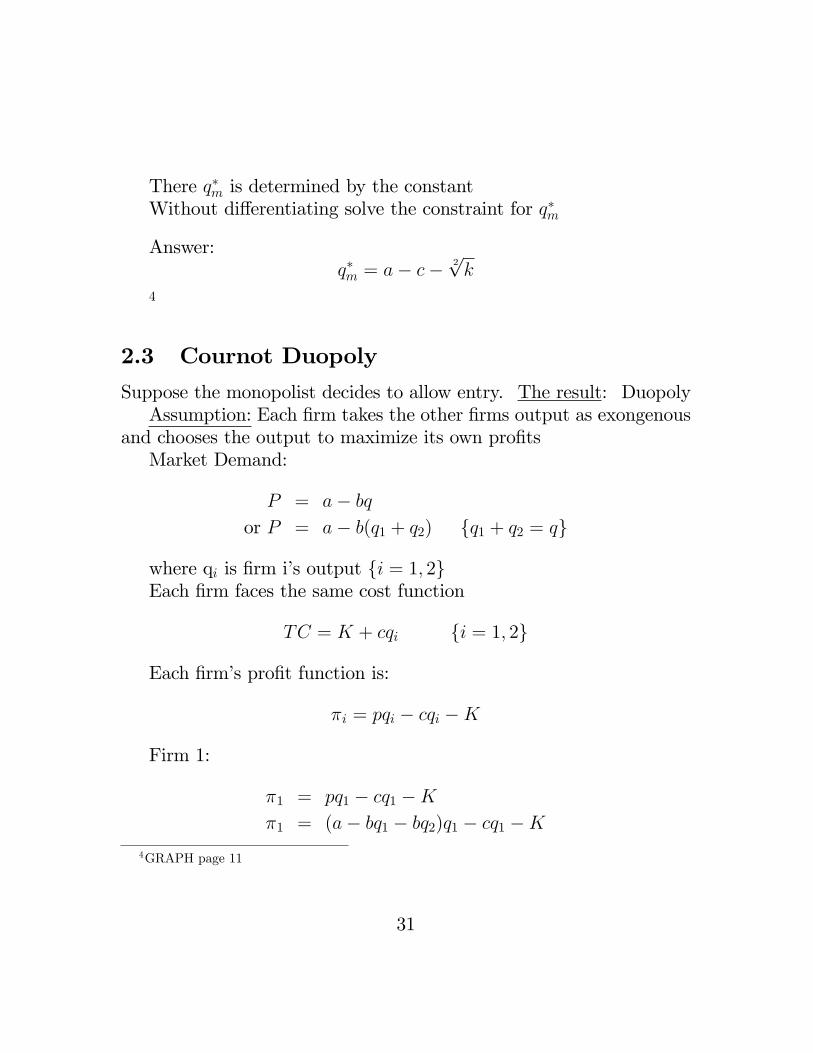
There q∗m is determined by the constantWithout differentiating solve the constraint for q∗m
Answer:q∗m = a− c− 2
√k
4
2.3 Cournot Duopoly
Suppose the monopolist decides to allow entry. The result: DuopolyAssumption: Each firm takes the other firms output as exongenous
and chooses the output to maximize its own profitsMarket Demand:
P = a− bqor P = a− b(q1 + q2) {q1 + q2 = q}
where qi is firm i’s output {i = 1, 2}Each firm faces the same cost function
TC = K + cqi {i = 1, 2}
Each firm’s profit function is:
πi = pqi − cqi −K
Firm 1:
π1 = pq1 − cq1 −Kπ1 = (a− bq1 − bq2)q1 − cq1 −K
4GRAPH page 11
31

Max π1, treating q2 as a constant
∂π1∂q1
= a− bq2 − 2bq1 − c = 0
2bq1 = a− c− bq2q1 =
a− c2b− q2
2−→ "Best Response Function"
Best Response Function: Tells firm 1 the profit maximizing q1 forany level of q2For Firm 2:
π2 = (a− bq1 − bq2)q2 − cq2 −K
Max π2 (treating q1 as a constant) gives
q2 =a− c
2b− q1
2Firm 2’s Best Response Function
The two "Best Response" Functions
(1) q1 = a−c2b −
q22
(2) q2 = a−c2b −
q12
gives us two equations and two unknowns.The solution to this system of equations is the equilibrium to the
"Cournot Duopoly" gameUsing Cramer’s Rule:
(1) q∗1 = a−c3b
(2) q∗2 = a−c3b
Market Output : q∗1 + q∗2 =2(a− c)
3b
Best Response Functions Graphically
32

2.4 Stackelberg Duopoly
In the Cournot Duopoly , 2 firms picked output simultaneously. Sup-pose firm 1 was able to choose output first, knowing how firm 2‘s outputwould vary with firm 1‘s output.
2.4.1 Firm 1‘s Max Problem
Max q1 : (a− bq1 − bq2)q1 − cq1 −KSubject to:
q2 =a− c
2b− q1
2{2’s Response Function}
33

Sub in for q2
Max q1 : aq1 − bq21 − bq1(a− c
2b− q1
2
)− cq1 −K
∂π1∂q1
= a− 2bq1 −(a− c
2b
)+ bq1 − c = 0
q∗1 =a− c
2b
Firm 2:
q2 =a− c
2b− q1
2Sub in
q1 =a− c
2b
q∗2 =a− c
2b− 1
2
(a− c
2b
)=a− c
4b
34

Graphically: Stackelberg and Cournot Equilibrium
35