primal dual approximation algorithms - microsoft.com · the basic paradigm many real-life problems...
TRANSCRIPT

Primal Dual Approximation AlgorithmsOr, Partially Covering topics in Partial Covering
Sambuddha Roy1
1IBM Research – India
Sambuddha Roy (IBM Research – India) Primal Dual January 2011 1 / 61

Outline
1 Motivation
2 The Primal Dual Schema
3 Vertex Cover
4 Prize Collecting Vertex Cover
5 Partial Vertex Cover
6 Lagrangian Relaxations
7 Ending Comments
Sambuddha Roy (IBM Research – India) Primal Dual January 2011 2 / 61

The Basic Paradigm
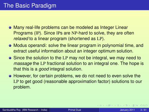
Many real-life problems can be modeled as Integer LinearPrograms (IP). Since IPs are NP-hard to solve, they are oftenrelaxed to a linear program (shortened as LP).Modus operandi: solve the linear program in polynomial time, andextract useful information about an integer optimum solution.Since the solution to the LP may not be integral, we may need tomassage the LP fractional solution to an integral one. The hope isthat this is a good integral solution.However, for certain problems, we do not need to even solve theLP to get good (reasonable approximation factor) solutions to ourproblem.
Sambuddha Roy (IBM Research – India) Primal Dual January 2011 3 / 61

The Basic Paradigm
Many real-life problems can be modeled as Integer LinearPrograms (IP). Since IPs are NP-hard to solve, they are oftenrelaxed to a linear program (shortened as LP).Modus operandi: solve the linear program in polynomial time, andextract useful information about an integer optimum solution.Since the solution to the LP may not be integral, we may need tomassage the LP fractional solution to an integral one. The hope isthat this is a good integral solution.However, for certain problems, we do not need to even solve theLP to get good (reasonable approximation factor) solutions to ourproblem.
Sambuddha Roy (IBM Research – India) Primal Dual January 2011 3 / 61

Primal Dual Algorithms
Over the years, the primal dual paradigm has been used for:Approximation Algorithms (bicriteria too)Semidefinite ProgramsOnline Algorithms... etc.
Sambuddha Roy (IBM Research – India) Primal Dual January 2011 4 / 61

Primal Dual Algorithms
Over the years, the primal dual paradigm has been used for:Approximation Algorithms (bicriteria too)Semidefinite ProgramsOnline Algorithms... etc.
Sambuddha Roy (IBM Research – India) Primal Dual January 2011 4 / 61

Primal Dual Algorithms
Over the years, the primal dual paradigm has been used for:Approximation Algorithms (bicriteria too)Semidefinite ProgramsOnline Algorithms... etc.
Sambuddha Roy (IBM Research – India) Primal Dual January 2011 4 / 61

Primal Dual Algorithms
Over the years, the primal dual paradigm has been used for:Approximation Algorithms (bicriteria too)Semidefinite ProgramsOnline Algorithms... etc.
Sambuddha Roy (IBM Research – India) Primal Dual January 2011 4 / 61

History
George Dantzig started linear programming, and his ideas containthe first germs of primal dual algorithms. The Hungarian methodwas an application of the paradigm.Edmonds (1965) gave the first (sophisticated) application of theparadigm in his work on maximum weight matchings in arbitrarygraphs.Bar-Yehuda and Even (1981) first enunciated the paradigm in theirwork on the weighted Vertex Cover problem.
Sambuddha Roy (IBM Research – India) Primal Dual January 2011 5 / 61

History
Agrawal, Klein and Ravi (1991) developed sophisticated primaldual algorithms for Steiner Network problems.Their paradigm was utilized by Goemans, Williamson in 1994 toprove a seminal 2-factor approximation algorithm for the SteinerForest problem and its prize collecting variant.Jain, Vazirani (1999,2001) showed the powerful use of LagrangianRelaxations in addition to Primal Dual to give constant factoralgorithms for Facility Location, k -Median.Garg (1996) gave a 3-factor approximation algorithm for thek -MST problem. Later, Chudak, Roughgarden, Williamson (2004)showed that this is an application of the Lagrangian Relaxationtechnique.Arora, Karakostas (2000) gave a (2 + ε)-factor algorithm for thesame problem; Garg (2005) gave a 2-factor approximation.
Sambuddha Roy (IBM Research – India) Primal Dual January 2011 6 / 61

History
For Prize Collecting Vertex Cover, Hochbaum (2002) showed a2-factor approximation. Later, Bar-Yehuda and others gave localratio algorithms for the same.For Partial Vertex Cover, Gandhi, Khuller and Srinivasan gave thefirst 2-factor approximation algorithms. Later, Mestre (2005)improved the running time of the algorithm.and lot more papers...
Sambuddha Roy (IBM Research – India) Primal Dual January 2011 7 / 61

Primal, Dual and Weak Duality
Consider a LP in n variables x1, · · · , xn, and with m constraints.
Primal
min∑
i
cixi
s.t. a11x1 + a12x2 + · · ·+ a1nxn ≥ b1
a21x1 + a22x2 + · · ·+ a2nxn ≥ b2
· · · · · · · · ·am1x1 + am2x2 + · · ·+ amnxn ≥ bm
for all i xi ≥ 0 .
The dual is an effort to construct the best lower bound for the primalobjective. The dual program will have a variable corresponding toevery constraint in the primal; a variable in the primal manifests itselfas a dual constraint.
Sambuddha Roy (IBM Research – India) Primal Dual January 2011 8 / 61

Primal, Dual and Weak Duality
Variables↔ Constraints.
Let z1, · · · , zm denote the dual variables. The dual is as follows:
Dual
max∑
j
bjzj
s.t. a11z1 + a21z2 + · · ·+ am1zm ≤ c1
a12z1 + a22z2 + · · ·+ am2zm ≤ c2
· · · · · · · · ·a1nz1 + a2nz2 + · · ·+ amnzm ≤ cn
for all j zj ≥ 0 .
Sambuddha Roy (IBM Research – India) Primal Dual January 2011 9 / 61

Primal, Dual and Weak Duality
Weak Duality formalizes the notion of “best" lower bound for the(minimization) primal.
Weak DualityFor every feasible solution ~x to the primal and ~z to the dual programs,the following holds: ∑
i
cixi ≥∑
j
bjzj
Proof :∑i
cixi ≥∑
i
(∑
j
ajizj)xi =∑i,j
ajixizj =∑
j
(∑
i
ajixi)zj ≥∑
j
bjzj
Sambuddha Roy (IBM Research – India) Primal Dual January 2011 10 / 61
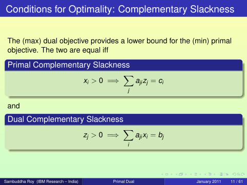
Conditions for Optimality: Complementary Slackness
The (max) dual objective provides a lower bound for the (min) primalobjective. The two are equal iff
Primal Complementary Slackness
xi > 0 =⇒∑
j
ajizj = ci
and
Dual Complementary Slackness
zj > 0 =⇒∑
i
ajixi = bj
Sambuddha Roy (IBM Research – India) Primal Dual January 2011 11 / 61

Relaxed Complementary Slackness
The idea behind the primal dual paradigm arises from the fact thatwe may relax the primal and dual slackness conditions in order toget approximation algorithms (instead of optimal algorithms).Suppose we have a set of feasible solutions (~x , ~z) for whichrelaxed dual slackness conditions hold, as follows:
Dual Complementary Slackness
zj > 0 =⇒∑
i
ajixi ≤ r · bj
for some factor r ≥ 1.
Sambuddha Roy (IBM Research – India) Primal Dual January 2011 12 / 61

Relaxed Complementary Slackness
Suppose also, that the primal feasible solution ~x is integral.Consider the following calculation (almost the same as that forWeak Duality).∑
i
cixi =∑
i
(∑
j
ajizj)xi =∑i,j
ajixizj =∑
j
(∑
i
ajixi)zj ≤ r ·∑
j
bjzj
Thus, by Weak Duality, the feasible solution ~x is a r -factorapproximation to the optimal, OPT. Why? Weak Duality implies∑
j bjzj ≤∑
i cix ′i for any feasible ~x ′, in particular for the optimal(integral) solution OPT. Thus∑
i
cixi ≤ r ·∑
j
bjzj ≤ r · OPT
We could also relax the primal slackness conditions, with a similarcalculation.
Sambuddha Roy (IBM Research – India) Primal Dual January 2011 13 / 61

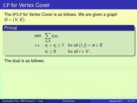
LP for Vertex Cover
The IP/LP for Vertex Cover is as follows. We are given a graphG = (V ,E).
Primal
min∑i∈V
cixi
s.t. xi + xj ≥ 1 for all (i , j) = e ∈ Exi ≥ 0 for all i ∈ V .
The dual is as follows:
Dual
max∑e∈E
ze
s.t. z(δ(i)) ≤ ci for all i ∈ Vze ≥ 0 for all e ∈ E .
Sambuddha Roy (IBM Research – India) Primal Dual January 2011 14 / 61

Rounding
Of course, we see that in the Vertex Cover LP above, for everyedge e ∈ E , we are guaranteed that one of the two endpoints xi orxj is ≥ 1/2.Thus, we may just round up the xi ’s that are ≥ 1/2. Easy to checkthat
1 The resulting (integer) solution is indeed a valid vertex cover.2 The cost of the solution is at most twice that of the LP value.
However, our goal (in this talk) is to use the primal dual paradigm.
Sambuddha Roy (IBM Research – India) Primal Dual January 2011 15 / 61

Primal Dual for Vertex Cover
Primal
min∑i∈V
cixi
s.t. xi + xj ≥ 1 for all (i , j) = e ∈ Exi ≥ 0 for all i ∈ V .
Dual
max∑e∈E
ze
s.t. z(δ(i)) ≤ ci for all i ∈ Vze ≥ 0 for all e ∈ E .
Start with the integerinfeasible primal solutionx = 0, and the feasibledual solution z = 0.Repeat while someconstraint in primal isunsatisfied:Increase all (unfrozen)variables ze until somedual constraint becomestight (say, for vertex i).Set xi = 1. Freeze all thevariables ze such that e isincident to i .
Sambuddha Roy (IBM Research – India) Primal Dual January 2011 16 / 61

In the end...
When the above process stops, we have increased the variablesze suitably.Some vertices i were chosen (indicated by xi = 1).This set of vertices is our output Vertex Cover.
Sambuddha Roy (IBM Research – India) Primal Dual January 2011 17 / 61

Proof?
The set S of vertices output is indeed a Vertex Cover. Why?Because we would have continued if some primal constraint werestill unsatisfied.Cost of the solution? This is where we arrive at the relaxedcomplementary slackness conditions.
Sambuddha Roy (IBM Research – India) Primal Dual January 2011 18 / 61
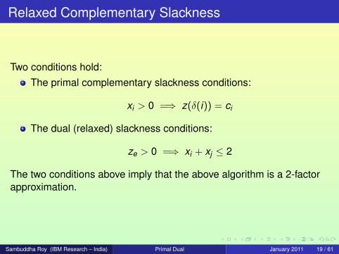
Relaxed Complementary Slackness
Two conditions hold:The primal complementary slackness conditions:
xi > 0 =⇒ z(δ(i)) = ci
The dual (relaxed) slackness conditions:
ze > 0 =⇒ xi + xj ≤ 2
The two conditions above imply that the above algorithm is a 2-factorapproximation.
Sambuddha Roy (IBM Research – India) Primal Dual January 2011 19 / 61

Further Comments
In the above algorithm, we increased the (active) dual variablessimultaneously.What we are essentially trying is to get the highest (the best) lowerbound that we can get for the primal minimization objective.We may also consider increasing the dual variables one-by-one.This would be a different algorithm (under the same primal dualparadigm). In the case of Vertex Cover, this also works to give a2-factor approximation.
Sambuddha Roy (IBM Research – India) Primal Dual January 2011 20 / 61
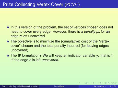
Prize Collecting Vertex Cover (PCVC)
In this version of the problem, the set of vertices chosen does notneed to cover every edge. However, there is a penalty pe for anedge e left uncovered.The objective is to minimize the (cumulative) cost of the “vertexcover" chosen and the total penalty incurred (for leaving edgesuncovered).The IP formulation? We will keep an indicator variable ye that is 1iff the edge e is left uncovered.
Sambuddha Roy (IBM Research – India) Primal Dual January 2011 21 / 61

PCVC: The LP relaxation
The primal LP is as follows:
Primal
min∑i∈V
cixi +∑e∈E
peye
s.t. xi + xj + ye ≥ 1 for all (i , j) = e ∈ Exi , ye ≥ 0 for all i ∈ V ,e ∈ E .
Dual
max∑e∈E
ze
s.t. z(δ(i)) ≤ ci for all i ∈ Vze ≤ pe for all e ∈ Eze ≥ 0 for all e ∈ E .
Sambuddha Roy (IBM Research – India) Primal Dual January 2011 22 / 61

Comments
What does rounding give? Each primal constraint now consists of3 variables, so some variable has to have value ≥ 1/3. Thisstraightaway gives a 3-factor approximation.On to primal dual.
Sambuddha Roy (IBM Research – India) Primal Dual January 2011 23 / 61

Rehash of earlier primal dual
Start with the integer infeasible primal solution ~x = ~0, ~y = ~0, andthe feasible dual solution ~z = ~0.Repeat while some primal constraint is unsatisfied:Increase all (unfrozen) variables ze until some dual constraintbecomes tight.However, here, we have two types of dual constraints, one ofwhich could have become tight
1 Either the constraint is of the type “z(δ(i)) ≤ ci ". In this case, we setxi = 1, and for all e ∈ E incident to i , we set ye = 0.
2 Or the constraint is of the type “ze ≤ pe". In this case, we set ye = 1and set xi = xj = 0 where e = (i , j).
Note that the algorithm (as stated so far) is a trivial extension ofthe primal dual algorithm that we presented for Vertex Cover.
Sambuddha Roy (IBM Research – India) Primal Dual January 2011 24 / 61

Issue in the algorithm for PCVC
However the following issue arises: At the end of the step above, itmay happen that for an edge e, we set ye = 1 first and then later,because of some constraint of the type “z(δ(i)) ≤ ci ", we end upsetting xi = 1 for i an endpoint of ye. As such, this would thereforegive us a 3-factor approximation.Delete Step Thus, we add the following last step: at the end of theprevious step, if xi = 1 for an endpoint i of an edge e such thatye = 1, then reset ye = 0.Now we are ready to do the analysis of the algorithm.
Sambuddha Roy (IBM Research – India) Primal Dual January 2011 25 / 61

Analysis
We will again check the relaxed complementary slackness conditions:Primal Complementary Slackness: If xi > 0, then z(δ(i)) = ci . Ifye > 0, then ze = pe.This is relatively clear from the algorithm..Dual Complementary Slackness: If ze > 0, then thecorresponding primal constraint xi + xj + ye ≤ 2. Why?
1 Either the constraint “z(δ(i)) ≤ ci " was made tight. In this case,xi + xj + ye ≤ 2, since ye was set equal to 0 for every e incident on i .
2 Or the constraint “ze ≤ pe" was made tight. In this case, observethat in the Delete Step of the algorithm, either ye was reset to 0(because some endpoint i of e was picked: xi = 1). In this case,xi + xj + ye ≤ 2. Or it was the case that ye retained its value of 1;thus, xi + xj + ye = 1.
Thus, what we have proven is · · ·
Sambuddha Roy (IBM Research – India) Primal Dual January 2011 26 / 61

More..
For the solution ~x , ~y generated by the above algorithm, thefollowing holds:
(∑i∈V
cixi +∑e∈E
peye) ≤ 2× (∑
e
ze)
But, by Weak Duality,∑
e ze ≤ OPT. Thus, the solution generatedis upper bounded by 2 ˙OPT.In fact more holds true:
(∑i∈V
cixi + 2∑e∈E
peye) ≤ 2× (∑
e
ze)
Why? Note that for the outcome generated by the algorithm,xi + xj + 2ye ≤ 2.
Sambuddha Roy (IBM Research – India) Primal Dual January 2011 27 / 61

PVC: Problem Definition
We will see that the stronger statement made above is preciselywhat is used for partial cover problems. This will take us into thedomain of Lagrangian relaxations. We will not go there, right yet.The Partial Vertex Cover (PVC) problem is the following: We aregiven a graph G = (V ,E) and a number k . A partial vertex coveris a set of vertices chosen such that the vertices cover at least kof the edges in the graph.We start by formulating the problem as an integer (linear)program.
Sambuddha Roy (IBM Research – India) Primal Dual January 2011 28 / 61

PVC: linear relaxation
Primal
min∑i∈V
cixi
s.t. xi + xj + ye ≥ 1 for all (i , j) = e ∈ E∑e∈E
ye ≤ s
xi , ye ≥ 0 for all i ∈ V ,e ∈ E .
Here, s = (m − k) is the maximum number of edges that can be leftuncovered by a valid (partial) vertex cover.
Sambuddha Roy (IBM Research – India) Primal Dual January 2011 29 / 61

PVC: a rewrite
For understanding the integrality gap of the relaxation, it might help toconsider the re-writing of the above LP.
Primal
min∑i∈V
cixi
s.t. xi + xj ≥ y ′e for all (i , j) = e ∈ E∑e∈E
y ′e ≥ k
y ′e ≤ 1 for all e ∈ Exi , y ′e ≥ 0 for all i ∈ V ,e ∈ E .
Here, we have just made the substitution y ′e = (1− ye). This makesthe LP look more “homogeneous".
Sambuddha Roy (IBM Research – India) Primal Dual January 2011 30 / 61

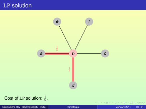
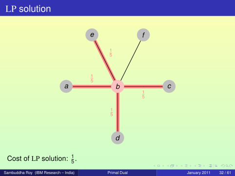
Integrality Gap
The LPs in the previous slide(s) have bad integrality gap.Consider the “star" graph K1,m, and let s = (m − 1) (i.e. k=1: onehas to cover just one edge). Let each vertex have cost ci = 1.An integer solution has to pick some vertex, and has a cost of 1.A fractional LP solution can pick the central vertex with xi = 1/m(every other vertex is given xj = 0), and for every edge, e, sety ′e = 1/m (i.e. ye = (m − 1)/m). Thus, the cost of this solution is1/m.Thus, there is a gap of Ω(m) between the optimal LP and theoptimal IP solution.
Sambuddha Roy (IBM Research – India) Primal Dual January 2011 31 / 61

LP solution
a b c
d
e f
b
Cost of LP solution: 15 .
Sambuddha Roy (IBM Research – India) Primal Dual January 2011 32 / 61

LP solution
15
a b c
d
e f
b
Cost of LP solution: 15 .
Sambuddha Roy (IBM Research – India) Primal Dual January 2011 32 / 61
LP solution
15
15
a b c
d
e f
b
Cost of LP solution: 15 .
Sambuddha Roy (IBM Research – India) Primal Dual January 2011 32 / 61

LP solution
15
15
15
a b c
d
e f
b
Cost of LP solution: 15 .
Sambuddha Roy (IBM Research – India) Primal Dual January 2011 32 / 61
LP solution
15
15
15
15
a b c
d
e f
b
Cost of LP solution: 15 .
Sambuddha Roy (IBM Research – India) Primal Dual January 2011 32 / 61

LP solution
15
15
15
15
15
a b c
d
e f
b
Cost of LP solution: 15 .
Sambuddha Roy (IBM Research – India) Primal Dual January 2011 32 / 61

IP solution
a b c
d
e f
b
Cost of IP solution: 1.
Sambuddha Roy (IBM Research – India) Primal Dual January 2011 33 / 61

Note however...
a b c
d
e f
a
If we had chosen the non-central vertices, then cost of LP solutionequals the cost of IP solution.
Sambuddha Roy (IBM Research – India) Primal Dual January 2011 34 / 61

Note however...
15
a b c
d
e f
a
d
If we had chosen the non-central vertices, then cost of LP solutionequals the cost of IP solution.
Sambuddha Roy (IBM Research – India) Primal Dual January 2011 34 / 61

Note however...
15
15
a b c
d
e f
a
d
c
If we had chosen the non-central vertices, then cost of LP solutionequals the cost of IP solution.
Sambuddha Roy (IBM Research – India) Primal Dual January 2011 34 / 61

Note however...
15
15
15
a b c
d
e f
a
d
c
f
If we had chosen the non-central vertices, then cost of LP solutionequals the cost of IP solution.
Sambuddha Roy (IBM Research – India) Primal Dual January 2011 34 / 61

Note however...
15
15
15
15
a b c
d
e f
a
d
c
fe
If we had chosen the non-central vertices, then cost of LP solutionequals the cost of IP solution.
Sambuddha Roy (IBM Research – India) Primal Dual January 2011 34 / 61

Note however...
15
15
15
15
15
a b c
d
e f
a
d
c
fe
If we had chosen the non-central vertices, then cost of LP solutionequals the cost of IP solution.
Sambuddha Roy (IBM Research – India) Primal Dual January 2011 34 / 61

Guide the LP
Thus, the LP can serve as a better lower bound, provided we giveit some guidance.What kind of guidance can we give it? Is the guidance "stay awayfrom high degree vertices"?Well, we are trying to cover edges, so this should not be theguidance.In order to uncover the guidance, let us play with the costs of thevertices. After all, they are what figure in the objective function.
Sambuddha Roy (IBM Research – India) Primal Dual January 2011 35 / 61
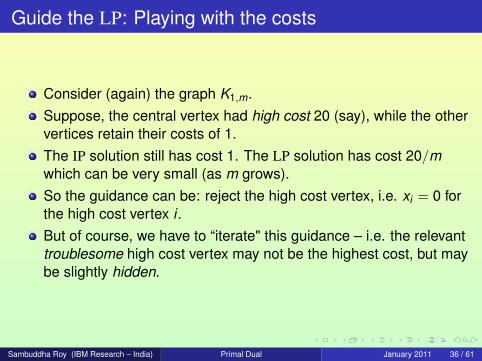
Guide the LP: Playing with the costs
Consider (again) the graph K1,m.Suppose, the central vertex had high cost 20 (say), while the othervertices retain their costs of 1.The IP solution still has cost 1. The LP solution has cost 20/mwhich can be very small (as m grows).So the guidance can be: reject the high cost vertex, i.e. xi = 0 forthe high cost vertex i .But of course, we have to “iterate" this guidance – i.e. the relevanttroublesome high cost vertex may not be the highest cost, but maybe slightly hidden.
Sambuddha Roy (IBM Research – India) Primal Dual January 2011 36 / 61

Guide the LP
Thus, the motto is:
GuidanceOrder the vertices by non-decreasing costs. Let this order bev1, v2, · · · , vn. Imagine disallowing the graph beyond vertex vi (i.e.guess that OPT does not have any vertex of cost higher than vi ). Solvethe modified LP.
Since we do not know the highest cost vertex in OPT, we will haveto guess it. Thus in effect we will have to solve n LPs.Note that the earlier integrality gap example vanishes now.So, are we in a better state now?
Sambuddha Roy (IBM Research – India) Primal Dual January 2011 37 / 61

Modified Algorithm
AlgoOrder the vertices by non-decreasing costs. Let the order bev1, v2, · · · , vn.Let h be the highest cost guessed vertex in OPT.Modify costs: For i > h, set c′i =∞; for i < h, set c′i = ci .Since we assume that vertex vh is in the desired optimum, updatek (the number of edges to be covered) as follows:k ′ = k − deg(vh). Remove vertex h from consideration.Run usual Vertex Cover (primal dual) algorithm on the residualgraph until k ′ edges are covered. Let the cover output be S.Output C = S ∪ h as the generated Vertex Cover.
Sambuddha Roy (IBM Research – India) Primal Dual January 2011 38 / 61

Analysis
Primal
min∑i∈V ′
cixi
s.t. xi + xj + ye ≥ 1 for all (i , j) = e ∈ E ′∑e∈E ′
ye ≤ s
xi , ye ≥ 0 for all i ∈ V ′,e ∈ E ′ .
Dual
max∑e∈E ′
ze − sλ
s.t. z(δ(i)) ≤ c′i for all i ∈ V ′
ze ≤ λze, λ ≥ 0 for all e ∈ E ′ .
Sambuddha Roy (IBM Research – India) Primal Dual January 2011 39 / 61

The usual Vertex Cover run on G′
Initialize Primal: Set all xi ’s to 0, all ye’s to 1. All the primalconstraints are satisfied but for the cardinality constraint.Initialize Dual: Set all ze = 0, set λ = 0.While all the constraints in the primal are not satisfied:
1 (Simultaneously) increase active dual variables ze such that somedual constraint (corresponding to vertex i ∈ V ′) becomes tight.
2 Set xi = 1, set ye = 0 for all e incident on vertex i .3 Check if
∑e ye ≤ s. If YES, STOP. If NO, continue.
Set λ = maxe ze.
Sambuddha Roy (IBM Research – India) Primal Dual January 2011 40 / 61

Analysis
Suppose OPT contains vh as the vertex of highest cost. Considerthe residual graph G′ on vertex set V ′ = V\vh, with modifiedcosts c′. Let E ′ denote the residual set of edges in G′.The costs c′ are modified as follows: For a vertex vt if ct > ch,then c′t =∞; else c′t = ct .Modify k as follows: k ′ (the coverage requirement on G′)= k − deg(vh). Note that the non-coverage requirement stays thesame, s.Note that we do not throw away vertices of higher cost. This isbecause they still may have edges incident on them that may beuseful for our solution.Let OPT′ denote the optimum on the graph G′. ThusOPT = OPT′ + ch.
Sambuddha Roy (IBM Research – India) Primal Dual January 2011 41 / 61

Analysis
Primal
min∑i∈V ′
cixi
s.t. xi + xj + ye ≥ 1 for all (i , j) = e ∈ E ′∑e∈E ′
ye ≤ s
xi , ye ≥ 0 for all i ∈ V ′,e ∈ E ′ .
Dual
max∑e∈E ′
ze − sλ
s.t. z(δ(i)) ≤ c′i for all i ∈ V ′
ze ≤ λze, λ ≥ 0 for all e ∈ E ′ .
Sambuddha Roy (IBM Research – India) Primal Dual January 2011 42 / 61

Analysis
Primal
min∑i∈V ′
cixi
s.t. xi + xj + ye ≥ 1 for all (i , j) = e ∈ E ′∑e∈E ′
ye ≤ s
xi , ye ≥ 0 for all i ∈ V ′,e ∈ E ′ .
Dual
max∑e∈E ′
ze − sλ
s.t. z(δ(i)) ≤ c′i for all i ∈ V ′
ze ≤ λze, λ ≥ 0 for all e ∈ E ′ .
Sambuddha Roy (IBM Research – India) Primal Dual January 2011 42 / 61

Analysis
In the run of the primal dual on the modified graph G′, let vl be thelast vertex chosen. Let S′ denote the other vertices chosen by theprimal dual algorithm (the final vertex cover output isC = S′ ∪ vl , vh).We will prove
Bound on c(S′)
c(S′) ≤ 2 · (∑e∈E ′
ze − sλ) ≤ 2 · OPT′
This proves the result (noting that cl ≤ ch):
Bound on output vertex cover
c(C) = c(S′) + cl + ch ≤ 2 · OPT′ + cl + ch ≤ 2 · (OPT′ + ch) = 2 · OPT
Sambuddha Roy (IBM Research – India) Primal Dual January 2011 43 / 61

Analysis – bound on c(S′)
Why did we have to choose the last vertex vl?Simply because, till that point
∑e ye > s still (not enough
coverage).But while choosing the last vertex vl , we do not change the dualvariables ze any more! Thus, the final λ is already set at this point.Let us consider the situation just before choosing the last vertex vl .
Sambuddha Roy (IBM Research – India) Primal Dual January 2011 44 / 61
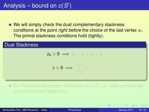
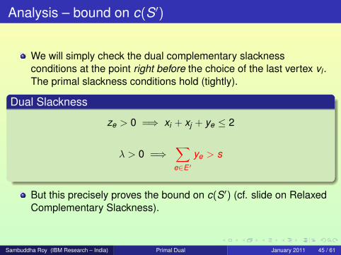
Analysis – bound on c(S′)
We will simply check the dual complementary slacknessconditions at the point right before the choice of the last vertex vl .The primal slackness conditions hold (tightly).
Dual Slackness
ze > 0 =⇒ xi + xj + ye ≤ 2
λ > 0 =⇒∑e∈E ′
ye > s
But this precisely proves the bound on c(S′) (cf. slide on RelaxedComplementary Slackness).
Sambuddha Roy (IBM Research – India) Primal Dual January 2011 45 / 61

Hindsight 20/20
Essentially, we compared the cost of an integer infeasible primalsolution with the feasible dual solution. Later, some of the yeswere turned to 0, lowering the cost even further.Why did we have to stop right before the last vertex vl chosen bythe algorithm? Could we not have enforced some complementaryslackness conditions then?It may be that the last vertex chosen causes lots of edges to bepicked up, so that
∑e ye falls down much below s. Thus, we might
not be able to get any sensible complementary slackness there.For instance, after the choice of the last vertex, it may be that∑
e ye = 0!Thus, the artifice of pinning down the algorithm at the “heaviest"(guessed) vertex is essentially to hedge such problems created bythe last vertex chosen by the algorithm.
Sambuddha Roy (IBM Research – India) Primal Dual January 2011 46 / 61

Back to Lagrangian Relaxations
Jain, Vazirani (2001) show how to use a prize collecting coveragealgorithm to construct a partial covering algorithm, usingLagrangian Relaxations.
PCVC with pe = α for all e
min∑i∈V
cixi +∑e∈E
αye
s.t. xi + xj + ye ≥ 1 for all (i , j) = e ∈ Exi , ye ≥ 0 for all i ∈ V ,e ∈ E .
PVC
min∑i∈V
cixi
s.t. xi + xj + ye ≥ 1 for all (i , j) = e ∈ E∑e∈E
ye ≤ s .
Sambuddha Roy (IBM Research – India) Primal Dual January 2011 47 / 61

From PCVC to PVC
Formulate a Lagrangian Relaxation of the PVC LP, taking theconstraint
∑e ye ≤ s into the objective function with a Lagrange
multiplier α.
Lagrangian Relaxation of PVC
min∑i∈V
cixi + α(∑
e
ye − s)
s.t. xi + xj + ye ≥ 1 for all (i , j) = e ∈ Exi , ye ≥ 0 for all i ∈ V ,e ∈ E .
The objective function “looks" like that of PCVC (with an extra αsfactor).This is a lower bound on PVC. Why? For PVC,
∑e ye ≤ s, thus,
the additional factor α(∑
e ye − s) is non-positive.
Sambuddha Roy (IBM Research – India) Primal Dual January 2011 48 / 61

From PCVC to PVC
Suppose we solve the PCVC problem
Lagrangian Relaxation of PVC: LPVC
min∑i∈V
cixi + α∑
e
ye
s.t. xi + xj + ye ≥ 1 for all (i , j) = e ∈ Exi , ye ≥ 0 for all i ∈ V ,e ∈ E .
via the primal dual algorithm, and the outcome happens to satisfy(for some α)
∑e ye = s.
Claim: The solution (partial) vertex cover generated is a 2-factorapproximation to the PVC problem.
Sambuddha Roy (IBM Research – India) Primal Dual January 2011 49 / 61

From PCVC to PVC
Let OPT′ denote the optimum integral value of LPVC, and OPTdenote that of PVC. Observe that
OPT′ ≤ OPT + αs
This is because: any feasible solution (~x , ~y) to PVC is also feasiblefor LPVC. The value of the optimum solution to PVC, looked uponas a feasible solution to LPVC is OPT + α
∑e ye ≤ OPT + αs. The
optimum solution to LPVC can only be lower than this (recall thatLPVC is a minimization problem).Now, note that for the LPVC run (for some α) we have that :∑
i∈V cixi + 2α∑
e ye ≤ 2OPT1
Thus,∑
i∈V cixi ≤ 2(OPT1 − αs) ≤ 2OPT.So, in the LPVC run, if it turns out that
∑e ye = s, then we are
done.Sambuddha Roy (IBM Research – India) Primal Dual January 2011 50 / 61

From PCVC to PVC
However, that may not happen. For different values of α, we mayend up getting
∑e ye < s or
∑e ye > s, but never equal.
In this case, run the LPVC primal dual algorithm for various valuesof α (in increasing order) and get two values α1 and α2(sufficiently close) such that for α1, the sum
∑e ye = s1 < s, while
for α2, the∑
e ye = s2 > s.There are two candidate vertex covers such that one covers toomany edges, and one covers too few edges.The idea then is to combine the two vertex covers to get a suitablevertex cover that covers at least k edges, at a small cost.
Sambuddha Roy (IBM Research – India) Primal Dual January 2011 51 / 61

Combining the two (partial) vertex covers
LPVC
min∑i∈V
cixi +∑e∈E
αye
s.t. xi + xj + ye ≥ 1 for all (i , j) = e ∈ Exi , ye ≥ 0 for all i ∈ V ,e ∈ E .
PVC
min∑i∈V
cixi
s.t. xi + xj + ye ≥ 1 for all (i , j) = e ∈ E∑e∈E
ye ≤ s .
Sambuddha Roy (IBM Research – India) Primal Dual January 2011 52 / 61

Combining the two (partial) vertex covers
Since the two values of α are sufficiently close, for brevity, we willassume them to be equal, i.e. α1 = α2 = α. Let OPTi (i = 1,2)denote the optimum value of the LPVC run with α = αi . Let OPTdenote the optimum value of PVC.Consider the two solutions C1 and C2. These have the followingproperties.
1 c(C1) + 2αs1 ≤ 2OPT1. Thus,c(C1) ≤ 2OPT1 − 2αs1 ≤ 2OPT + 2α(s − s1)
2 c(C2) + 2αs2 ≤ 2OPT2. Thus,c(C2) ≤ 2OPT2 − 2αs2 ≤ 2OPT + 2α(s − s2)
3 s1 < s < s2 (thus, for instance, c(C2) < 2OPT.
Sambuddha Roy (IBM Research – India) Primal Dual January 2011 53 / 61

Combining the two (partial) vertex covers
Since s is the non-coverage requirement, the solution C1 (thatleaves s1 < s edges uncovered) is feasible, but may be muchcostlier than 2OPT; while C2 is infeasible, but is actually upperbounded by 2OPT.We will consider a convex combination of the two solutions C1 andC2.
Sambuddha Roy (IBM Research – India) Primal Dual January 2011 54 / 61

Convex Combination of C1 and C2
Let β = s−s1s2−s1
. Thus, (1− β) = s2−ss2−s1
.Thus it follows that
(1− β)c(C1) + βc(C2) ≤ 2OPT
If β < 1/2 (i.e. (1− β) ≥ 1/2, then C1 is the major component inthis convex combination. and c(C1) ≤ 4OPT; since C1 is actuallyfeasible, we can output this as the solution.Suppose then that β > 1/2. In this case, we have to augment C2with (some part of C1) to get a feasible solution of cost ≤ 5OPT.
Sambuddha Roy (IBM Research – India) Primal Dual January 2011 55 / 61

Convex Combination of C1 and C2
Why did we not face the earlier issue of high cost vertices?Well, that figures in the last mentioned augmentation of C2 bysome part of C1. We will have to assume here that every vertexinvolved has cost ≤ OPT/2 (or something to that effect).Optimizing the parameters in the above gives a 8/3-factorapproximation for PVC.
Sambuddha Roy (IBM Research – India) Primal Dual January 2011 56 / 61

Remarks
Konemann, Parekh and Segev (2006) showed that given asuitable primal dual r -factor algorithm for the prize collectingvariant of a covering problem as a blackbox, one can design a4r/3-factor algorithm for the partial covering variant. (This is whatgave the 8/3 above).Mestre (2008) showed that this extra factor of 4/3 is inherent,whenever one uses such a primal dual algorithm as a blackbox.Thus, for instance, for the k -MST problem, Garg (1996) showed a3-factor approximation, while the underlying prize collectingSteiner tree problem has a 2-factor approximation. It requiredbreaking the blackbox and dealing with intricate details of theprimal dual algorithm for the prize collecting Steiner tree problemin order to bring the factor down to 2 (Garg, 2001).
Sambuddha Roy (IBM Research – India) Primal Dual January 2011 57 / 61

Remarks
In this talk, we did not mention the Local Ratio paradigm fordesigning approximation algorithms. The local ratio paradigm wasfirst described by Bar-Yehuda and Even in 1982. Algorithms forvarious problems were designed using the local ratio paradigm(for instance, for Feedback Vertex Set, Job Interval SelectionProblem, etc.).The paradigm essentially reduces a weighted problem to theunweighted version. Thus, it involves changing the weights (incase of Vertex Cover, the weights ci ) of an instance, to derive anew (simpler) instance.It was somewhat mysterious that problems that had algorithms inthe primal dual schema turned out to have local ratio algorithmsand vice versa.In 2005, Bar-Yehuda and Rawitz proved the formal equivalence ofthe two techniques.
Sambuddha Roy (IBM Research – India) Primal Dual January 2011 58 / 61

Remarks
While Primal Dual algorithms work with an underlying LP and itsdual, they do not require to actually solve the LP. Thus, most ofsuch algorithms are rather fast, and are combinatorial in nature.Comparison with other paradigms: Iterative Rounding vs. PrimalDual. The two techniques showed up a sharp contrast for theMBDST problem: primal dual only gave a O(log n) additiveapproximation, whereas iterative rounding gave the optimal +1approximation (Singh, Lau).On the other hand, for problems like Job Interval SelectionProblem, iterative rounding does not give much.
Sambuddha Roy (IBM Research – India) Primal Dual January 2011 59 / 61

Thanks
Thanks!
Sambuddha Roy (IBM Research – India) Primal Dual January 2011 60 / 61

For Further Reading I
A. Author.Handbook of Everything.Some Press, 1990.
S. Someone.On this and that.Journal of This and That, 2(1):50–100, 2000.
Sambuddha Roy (IBM Research – India) Primal Dual January 2011 61 / 61