pricing and hedging spread options · pricing and hedging spread options ... of electricity trading...

PRICING AND HEDGING SPREAD OPTIONS

RENE CARMONA AND VALDO DURRLEMAN

ABSTRACT. We survey the theoretical and the computational problems associated with the pricing ofspread options. These options are ubiquitous in the financial markets, whether they be equity, fixedincome, foreign exchange, commodities, or energy markets. As a matter of introduction, we present ageneral overview of the common features of all the spread options by discussing in detail their rolesas speculation devices and risk management tools. We describe the mathematical framework used tomodel them and we review the numerical algorithms used to actually price and hedge them. There isalready an extensive literature on the pricing of spread options in the equity and fixed income markets,and our contribution there is mostly to put together material scattered across a wide spectrum of recenttext books and journal articles. On the other hand, information about the various numerical procedureswhich can be used to price and hedge spread options on physical commodities is more difficult to find.For this reason, we make a systematic effort to choose examples from the energy markets in order toillustrate the numeric challenges associated with these instruments. This gives us a chance to venturein the poorly understood world of asset valuation and real options which are the object of a frenzy ofactive mathematical research. In this spirit, we review the two major avenues to modeling energy pricesdynamics, and we explain how the pricing and hedging algorithms can be implemented both in theframework of models for the spot prices dynamics as well as for the forward curves dynamics.

1. I NTRODUCTION

Whether the motivation comes from speculation, basis risk mitigation, or even asset valuation, theuse of spread options1 is widespread despite the fact that the development of pricing and hedgingtechniques has not followed at the same pace. These options can be traded on an exchange, butthe bulk of the volume comes from over the counter trades. They are designed to mitigate adversemovements of several indexes, hence their popularity. Because of their generic nature, spread optionsare used in markets as different as the fixed income markets, the currency and foreign exchangemarkets, the commodity futures markets and the energy markets.

One of our goals is to review the literature existing on the subject, including a self-containeddiscussion of all the pricing and hedging methodologies known to us. We implemented all the pricingalgorithms whose existence we are aware of, and for the purpose of comparison, we report on theirnumerical performances and we give evidence of their relative accuracy and computing times.

As evidenced by the title of the paper, we intend to concentrate on the energy markets. Standardstock market theory relies on probabilistic models for the dynamics of stock prices, and uses arbi-trage arguments to price derivatives. In most models, futures and forward contract prices are simplythe current (spot) price of the stock corrected for growth at the current interest rate. This simple

Date: February 22, 2003.1The spread option is a set play in American football, and a lot of write ups have been devoted to its analysis and to its

merits. Despite its importance in the life of football fans, we shall ignore this popular type of spread option and concentrateinstead on the analysis of the spread options traded in the financial markets.

1

2 RENE CARMONA AND VALDO DURRLEMAN

relationship between spot and forward prices does not hold in the commodity markets, and we willrepeatedly mention seasonality and mean reversion as main culprits. In order to reconcile the physi-cal commodity market models with its equity relatives, researchers have used several tricks to resolvethis apparent anomaly, and consistency with the no-arbitrage theory is restored most often by addingcost of storage and convenience yields to the stochastic factors driving the models. See,e.g., [20],[8], [41], [24] and [36]. But the main limitation of these methods is the inherent difficulties in mod-eling these unobserved factors (storage costs and especially convenience yield for example) and theproposal to use stochastic filtering techniques to estimates them, even though very attractive, did notfully succeed in resolving these problems.

Beyond the synthesis of results from a scattered technical literature, our contribution to the subjectmatter is the introduction of a new pricing algorithm based on closed form formulae providing lowerbounds to the exact values of the spread options when the distributions of the underlying indexes arelog-normal. We construct our approximate prices rigorously, we derive all the formulae necessary tothe numerical implementation of our algorithm, and we demonstrate its efficiency on simulations andpractical examples. All of the practical applications considered in this paper for the sake of illustrationare from the energy markets.

The energy markets have seen rapid changes in the last decade, mostly because of the introductionof electricity trading and the restructuring of the power markets. The diversity in the statistical char-acteristics of the underlying indexes on which the financial instruments are defined, together with theextreme complexity of the derivatives traded, make the analysis of these markets an exciting challengeto the mathematically inclined observer. This paper came out of our curiosity in these markets, andour desire to better understand their idiosyncrasies. The reader is referred to [15] for a clear initiationto the intricacies of the energy markets, and to the recent texts [26], [43] and [3] for the economic andpublic policy issues specific to the electricity markets. But our emphasis will be different since we areonly concerned with the technical aspects of energy trading and risk management. Several textbooksare devoted to the mathematical models of and risk management issues in the energy markets. Themost frequently quoted are [37] and [7], but this may change with the publication of the forthcomingbook [16]. Even though this paper concentrates on the spread options and [7] does not deal withcross-commodity instruments, we shall use many of the models and procedures presented in [7]. Weclose this introduction with a summary of the contents of the paper.

The paper starts with a review of the various forms of spread options in Section 2. We give ex-amples of instruments traded in the equity, fixed income and commodity markets. Understandingthis diversity is paramount to understanding the great variety of mathematical models and of pricingrecipes which have appeared in the technical literature. In preparation for our discussion of the prac-tical examples discussed in the last sections of the paper, we devote Section 3 to a detailed discussionof the data available to the energy market participants. The special characteristics of these data shouldnot only justify the kind of notation and assumptions we use, but it should also serve as a yardstick toquantify how well the pricing algorithms do.

The mathematical framework for risk-neutral pricing of spread option is introduced in Section 4.Even though most of the spread options require only the statistics of the underlying indexes at onesingle time, namely the time of maturity of the option, these statistics are usually derived from a modelof the time evolution of the values of the indexes. See nevertheless our short discussion of the calendarspreads where the joint distribution of the same underlying index at different times is needed. We

SPREAD OPTIONS 3

introduce the stochastic differential equations used to model the dynamics of the underlying indexes.The price of a spread option is given by an expectation over the sample paths of the solution of thissystem of stochastic differential equations. One usually assumes that the coefficients of the stochasticdifferential equations are Markovian. In this case, the price is easily seen to be the solution of aparabolic partial differential equation. This connection between solutions of stochastic differentialequations and solutions of partial differential equations is a cornerstone of Ito’s stochastic calculus,and it has been exploited in many financial applications. Only in very exceptional situations do theseequations have solutions given by closed form formulae. PDE solvers, tree methods and Monte Carlomethods are most commonly used to produce numerical values approximating the price of a spread.Because the applied mathematics community is more familiar with PDE solvers than with the othertwo, we spend more time reviewing the tree and Monte Carlo methods and the specifics of theirimplementations in the pricing of spread options. Also, we address the issue of the quantification ofthe dependencies of the price with respect to the various parameters of the model. We emphasize thecrucial role of these sensitivities in a risk management context by explaining their roles as hedgingtools.

As seen from the discussion of that section, the model of utmost importance is the Samuelson’smodel in which the distributions at the time of maturity of the indexes underlying the spread optionare log-normal. We shall concentrate most of our efforts in understanding the underpinnings of thisassumption on the statistics of the indexes.

The following Section 5 presents the first approximation procedure leading to a full battery ofclosed form expressions for the price and the hedging portfolios of a spread option with general strikepriceK. It is based on a simple minded remark: as evidenced by a quick look at empirical samples,the distribution of the difference between two random variables with log-normal distributions lookspretty much like a normal distribution. This is the rationale for the first of the three approximationmethods which we review. In this approach, one refrains from modeling the distributions of theindexes separately and instead, one models the distribution of their difference. As we just argued, itis then reasonable to assume that the latter is normally distributed. This model is called the Bacheliermodel because it is consistent with a model of the spread dynamics based on a single Brownianmotion, in the same way Bachelier originally proposed to model the dynamics of the value of a stockby a continuous time process generalizing the notion of random walk. Little did he knew he was aheadof Einstein introducing the process of Brownian motion. We give a complete analysis of this model.We derive explicit formulae for the option prices in the original form of the model, and when themodel is adjusted for consistency with observed forward curves. In this section, we also examine indetail the numerical performance of the pricing formula, by comparing its results to the exact valueswhen the driving dynamics are actually given by geometric Brownian motions as in the Samuelson’smodel which we study next.

In Section 6 we turn our attention to the particular case of a spread option with log-normal indexesand strikeK = 0. Like in the case of the Bachelier’s model, it is possible to give a Black-Scholestype formula for the price of the option. This formula was first derived by Margrabe in [33]. It cannotbe extended to the general caseK > 0, and this is the main reason for the investigations which wereview in this paper. Besides the fact that the caseK = 0 leads to a solution in closed form, it hasalso a practical appeal to the market participants. Indeed, it can be viewed as an option to exchange aproduct for another. Let us imagine for the sake of illustration, that we are interested in owning at a


given timeT in the future, either one of two instruments whose prices at timet we denote byS1(t)andS2(t), and that the choice of which one to buy has to be done now at timet = 0. If we fear thatthe difference in price may be significant at timeT , choosing the second instrument and buying thespread option with strikeK = 0 is the best way to guarantee that we will end up financially in thesame situation as we had chosen in hindsight the instrument which will end up been the cheaper attimeT . The only cost to us will be the purchase of the spread option. Indeed, if the second instrumentends up being the most expensive, i.e. ifS2(T ) > S1(T ), then the pay-offS2(T ) − S1(T ) of theoption will compensate us for our wrong choice.

The main mathematical thrust of the paper is contained in Section 7 where we review the recentresults of Carmona and Durrleman [5], and where we compare the numerical performance of theirmethod to the approximations based on the Bachelier’s approach and the Kirk’s approximate pricingformula. The basic problem is the pricing and hedging of the simplest spread option (i.e., an Euro-pean call option on the difference of two underlying indexes) when the risk-neutral dynamics of thevalues of the underlying indexes are given by correlated geometric Brownian motions. The resultsof Carmona and Durrleman are based on a systematic analysis of expectations of functions of linearcombinations of log-normal random variables. The motivation for this analysis comes from the grow-ing interest in basket options, whose pricing involves the computation of these expectations when thenumber of log-normal random variables is large. These products are extremely popular, as they areperceived as a safe diversification tool. But a rigorous pricing methodology is still missing. The au-thors of [5] derive lower bounds in closed form, and they propose an approximation to the exact valueof these expectations by optimizing over these lower bounds. The performance of their numericalscheme is always as good as the results of Kirk’s formula. But the main advantage of their approachis the fact that it also provides a set of approximations for all the sensitivities of the spread optionprice, an added bonus making possible risk management at the same time. We review the propertiesof these approximations, both from a theoretical and a numerical point of view by quantifying theaccuracy on numerical simulations. The reader interested in detailed proofs and extensive numericaltests is referred to [5].

The geometric Brownian motion assumption of the Samuelson’s theory is not realistic for mostof the spread options traded in the energy markets. Indeed, most energy commodity indexes have astrong seasonal component, and they tend to revert to a long term mean level, this mean level havingthe interpretation ofcost of production.These features are not accounted for by the plain geometricBrownian motion model of Samuelson. Section 8 deals with the extension of the results of Section 7to the case of spread options on the difference of indexes whose risk-neutral dynamics include thesefeatures. We also show how to include jumps in the dynamics of these indexes. This is motivated bythe pricing of spark spread options which involve electricity as one of the two underlying indexes, orthe pricing of calendar spread options on electric power.

Up until Section 9, we only work with stochastic differential equation models for the indexesunderlying the spread. In the case of the energy markets, the natural candidates for these underlyingindexes are the commodity spot prices, and these models are usually called spot price models. Seee.g., Chapters 6 and 7 of [7]. According to the prevailing terminology, they are one-factor modelsfor the term structure of forward prices. But it should be emphasized that our analysis extends easily,and without major changes, to the multi-factor models, at least as long as the distributions of theunderlying indexes can be constructed from log-normal building blocks. This is the case for most of

SPREAD OPTIONS 5

the models used in the literature on commodity markets. See,e.g., [20], [8], [41], [24], [36] or [37]and [7].

Most of the energy commodities do not behave much differently than the other physical commodi-ties. They share the mean reversion feature which we will mention quite often in this paper, butsurprisingly enough, some do not exhibit much seasonality. This is the case for crude oil for exam-ple. But beyond natural gas whose historical data are readily available and which exhibits strongseasonality and mean reversion, one of these commodities does stand out because of its very specialfeatures: electric power. Indeed, its price is function of factors as diverse as 1) instant perishableness,2) strong demand variations due to seasonality and geographic location, 3) extreme volatility and sud-den fluctuations caused by weather changes in temperature, precipitation,. . . 4) physical constraints inproduction (start-ups, ramp-ups) and transmission (capacity constraints). It is by far the most difficultcommodity index to model and predict. Derivative pricing and risk management present challengesof a new dimension: but what appears to be a nightmare for policy makers and business executives, isin fact a tremendous opportunity for the academic community, and the need for realistic mathematicalmodels and rigorous analytics is a very attractive proposition for the scientific community at large.

The last section of the paper is concerned with forward curve models. Using ideas from the HJMtheory developed for the fixed income markets, the starting point of Section 9 is a set of equations forthe stochastic dynamics of the entire forward curve. This is a departure from the approach used in theprevious sections, where the dynamics of the spot prices were modeled, and where the consistencywith the existing forward curves was only an after thought. We give a detailed account of the fittingprocedure based on Principal Components Analysis (PCA for short) and we illustrate the numericalperformance of this calibration method using real data. Restricting the coefficients of the stochasticdifferential equations to be deterministic leads again to log-normal distributions and the results re-viewed in this paper can be applied. We show how to price calendar spreads and spark spreads in thisframework.

Acknowledgements:The authors thank Bobray Bordelon for providing us with data of DatastreamInternational. Also we would like to thank David Doyle and Dario Villani for enlightening discussionsduring the preparation of the manuscript.

2. ZOOLOGY OF THE SPREAD OPTIONS

Even though it is sometime understood as the difference between the bid and ask prices (for exam-ple one often says that liquid markets are characterized by narrow bid/ask spreads), the term spreadis most frequently used for the difference between two indexes: the spread between the yield of acorporate bond and the yield of a Treasury bond, the spread between two rates of returns,. . . aretypical examples. Naturally, a spread option is an option written on the difference between the valuesof two indexes. But as we are about to see, its definition has been loosened to include all the formsof options written on a linear combination of a finite set of indexes. In the currency and fixed incomemarkets, spread options are based on the difference between two interest or swap rates, two yields,. . . . In the commodity markets, spread options are based on the differences between the prices ofthe same commodity at two different locations (location spreads), or between the prices of the samecommodity at two different points in time (calendar spreads), or between the prices of inputs to, andoutputs from, a production process (processing spreads) as well as between the prices of different


grades of the same commodity (quality spreads). The New York Mercantile Exchange (NYMEXfor short) offers the only exchange-traded options on energy spreads: the heating oil/crude oil andgasoline/crude oil crack spread options.

The following review is far from exhaustive. It is merely intended to give a flavor of the diversityof spread instruments in order to justify the variety of mathematical models and pricing algorithmsfound in the technical literature on spreads. In this paper, most of the emphasis is placed on cross-commodity spreads because of the tougher mathematical challenges they present. As we shall see,single commodity spreads (typically calendar spreads) are usually easier to price.

2.1. Spread Options in the Currency and Fixed Income Markets.Spread options are quite com-mon in the foreign exchange markets where spreads involve interest rates in different countries. TheFrench-German and the Dutch-German bond spreads are used because the economies of these coun-tries are intimately related. A typical example is the standard cross-currency spread option whichpays at maturityT the amount(αY1(T ) − βY2(T ) −K)+ in currency1. Hereα, β andK are pos-itive constants, and we use the notationx+ for the positive part ofx, i.e., x+ = max{x, 0}. Theunderlying indexesY1 andY2 are swap rates in possibly different currencies, say2 and3. The pricingof these spread options is usually done under some form of log-normality assumption via numeri-cal integration of Margrabe formulae derived in Section 6 below. The more elaborate forms of thisapproach are used to price quanto-swaptions as described for example in [4].

In the US fixed income market, the most liquid spread instruments are spreads between maturities,such as the NOB spread (Notes - Bonds) and spreads between quality levels, such as the TED spread(Treasury Bills - EuroDollars). The MOB spread measures the difference between Municipal Bondsand Treasury Bonds. See [1] for an econometric analysis of the market efficiency of these instruments.Spreads between Treasury Bills and Treasury Bonds have been studied in [29] and [14]. A detailedanalysis of a spread option between the three months and the six months LIBOR’s (London InterBank Overnight Rate) is given in [5] where some of the mathematical tools reviewed of this paperwere introduced.

2.2. Spread Options in the Agricultural Futures Markets. There are several spread options tradedin the agricultural futures markets. For the sake of definiteness, we decided to concentrate on the so-calledcrush spreadtraded on the Chicago Board of Trade (CBOT). It is also known as thesoybeancomplex spread.The underlying indexes comprise futures contracts of soybean, soybean oil andsoybean meal. The unrefined product is the soybean, and the derivative products are the meal andthe oil. This spread is known as thecrush spreadbecause soybeans are processed by crushing. Thesoybean crush spread is defined as the value of meal and oil extracted from a bushel of soybeans,minus the price of a bushel of soybeans. Notice that the computation of the spread requires threeprices as well as the yield of oil and meal per bushel. The crush spread gives market participants anindication of the average gross processing margin. It is used by processors to hedge cash positions orfor pure speculation.

The crush spread relates the cash market price of the soybean products (meal and oil) to the cashmarket price of soybeans. Since soybeans, soybean meal, and soybean oil are priced differently, con-version factors are needed to equate them when calculating the spread. On the average, crushing onebushel (i.e., 60 pounds) of soybeans produces48 pounds of meal and11 pounds of oil. Consequently,

SPREAD OPTIONS 7

the value[CS]t at timet of the crush spread in dollars per bushel can be defined as:

(1) [CS]t = 48[SM ]t/2000 + 11[SO]t/100− [S]t

where [S]t is the futures price at timet of a soybean contract in dollars per bushel,[SO]t is thefutures price at timet of a contract of soy oil in dollars per100 pounds, and[SM ]t is the price attime t of a soy meal contract in dollars per ton. In the terminology and the notation introduced belowfor the crack spreads, the spread described above is a 10:11:9 spread,i.e., 10 Soybean futures,11Soybean Meal futures, and9 Soybean Oil futures. So if we think of the crushing cost as a constantK, then crushing soybeans is profitable when the spread[CS]t is greater thanK. The crush spreadwas analyzed from the point of view of market efficiency in [28].

2.3. Spread Options in the Energy Markets. In the energy markets, beside thetemporal spreadtraders who try to take advantage of the differences in the prices of the same commodity at two differ-ent dates in the future, and thelocational spreadtraders who try to hedge transportation/transmissionrisk exposure from futures contracts on the same commodity with physical deliveries at two differentlocations, most of the spread traders deal with at least two different physical commodities. In the en-ergy markets spreads are typically used as a way to quantify the cost of production of refined productsfrom the complex of raw material used to produce them. The most frequently quoted spread optionsare the crack spread options and the spark options which we review in detail in this section. Crackspreads are often called paper refineries while spark spreads are sometimes called paper plants.

Crack Spreads. A crack spreadis the simultaneous purchase or sale of crude against the sale orpurchase of refined petroleum products. These spread differentials which represent refining marginsare normally quoted in dollars per barrel by converting the product prices into dollars per barrel andsubtracting the crude price. They were introduced in October 1994 by the NYMEX with the intendto offer a new risk management tool to oil refiners.

For the sake of illustration, we describe the detailed structure of the most popular crack spread con-tracts. These spreads are computed on the daily futures prices of crude oil, heating oil and unleadedgasoline.

• The3 : 2 : 1 crack spread involves three contracts of crude oil, two contracts of unleadedgasoline, and one contract of heating oil. Using self-explanatory notation, the defining for-mula for such a spread can be written as:

(2) [CS]t =23[UG]t +

13[HO]t − [CO]t

which means that at any given timet, the value (in US $)[CS]t of the3 : 2 : 1 crack spreadunderlying index is given by the right hand side of formula (2) where[UG]t, [HO]t and[CO]t denote the prices at timet of a futures contract of unleaded gasoline, heating oil andcrude oil respectively. A modicum of care should be taken in the numerical implementation offormula (2) with real data. Indeed, crude oil prices are usually quoted in “dollars per barrel”while unleaded gasoline and heating oil prices are quoted in “dollars per gallon”. A simpleconversion needs to be applied to the data using the fact that there are42 gallons per barrel,but it should not be overlooked.


• The1 : 1 : 0 gasoline crack spreadinvolves one contract of crude oil and one contract ofunleaded gasoline. Its value is given by the formula:

(3) [GCS]t = [UG]t − [CO]t• The1 : 0 : 1 heating oil crack spreadinvolves one contract of crude oil and one contract of

heating oil. It is defined as:

(4) [HOCS]t = [HO]t − [CO]tNotice that the first example is computed from three underlying indexes while the remaining twoexamples involve only two underlying indexes. Most of our analysis will concentrate on spreadoptions written on indexes computed from two underlying indexes.

Crack spread options are the subject of a large number of papers attempting to demonstrate thestationarity of the spread time series by means of a statistical quantification of the co-integrationproperties of underlying index time series comprising the spread. Most of these papers are alsoconcerned with the profitability of spread based trading strategies, subject which we would not dareto consider here. The interested reader is referred for example to [21], and [22] and the referencestherein for further information on these topics.

Spark Spreads. A spark spreadis a proxy for the cost of converting a specific fuel (most of the time,natural gas) into electricity at a specific facility. It is the primary cross-commodity transaction in theelectricity markets. Mathematically, it can be defined as the difference between the price of electricitysold by a generator and the price of the fuel used to generate it, provided these prices are expressedin appropriate units. The most commonly traded standardized contracts include:

• The4 : 3 spark spread involves four electric contracts and three contracts of natural gas. Itsvalue is given by:

(5) [SS]4,3t = 4[E]t − 3[NG]t

• The5 : 3 spark spreadwhich involves five electric contracts and three contracts of naturalgas. Its value is given by:

(6) [SS]5,3t = 5[E]t − 3[NG]t.

But whether or not they are traded in this form, the most interesting spread options are European callson an underlying index of the form:

St = FE(t)−HeffFG(t)

whereFE(t) andFG(t) denote the prices of futures contracts on electric power and natural gas re-spectively, and whereHeff is the heat rate, or the efficiency factor of a power plant. One of the mostintriguing use of spark spread options is in real asset valuation or capacity valuation. This encapsu-lates the economic value of the generation asset used to produce the electricity. The spark spread canbe expressed in $/MWh (US dollar per Mega Watt hour) or any other applicable unit. It is calculatedby multiplying the price of gas, (for example in $/MMBtu), by theheat rate(in Btu/KWh), dividingby 1, 000, and then subtracting the electricity price (in $/MWh). The heat rate is often called theefficiency.Indeed, a natural gas fired unit can be viewed as a series of spark spread options:

• when the heat rate implied by the spot prices of power and gas is above the operating heatrate of the plant, then the plant owner should buy gas, produce power, and sell it for profit.

SPREAD OPTIONS 9

• the plant owner should shut down its operation otherwise,i.e., when the heat rate implied bythe spot prices of power and gas is below the operating heat rate of its plant.

If an investor/producer wonders how much to bid for a power plant, he can easily estimate and predictthe real estate and the hardware values of the plant with standard methods. But the operational valueof the plant is better captured by the sum of the prices of spark spread options, than with the presentvalue method based on the computation of discounted future cash flows (the so-called DCF methodin the jargon of the business.) Thisreal optionapproach to the plant valuation is one of the strongestincentive to develop a better understanding of the basis risk of spark spread options.

3. M ARKET DATA

The purpose of this section is to demonstrate why some of the financial derivatives used in theenergy markets need to be treated with a modicum of care, by which we mean that applying blindlythe tools developed for the equity or fixed income markets may not be appropriate. Most of the math-ematical models used in the equity markets are based on generalizations of the geometric Brownianmotion model first proposed by Samuelson. We shall use these models in several instances, mostlyfor the sake of completeness since they are not of great use in the applications we consider. Energymarket models bare more resemblance to the models for the fixed income markets where there is adivision between the models for the dynamics of the short interest rate, and the models for the dynam-ics of the entire yield curve. This dichotomy will appear below where we divide the energy marketsmodels into two classes, the first one based on the dynamics the spot market prices, and the secondclass based on models for the dynamics of the entire forward curve. But in order to justify the specificassumptions we use, it is important to get a good understanding of the kind of data analysts, riskmanagers, traders,. . . are dealing with.

For most physical commodities, price discovery takes two different forms. The first one is back-ward looking. It is based on the analysis of a time series of historical prices giving the values observedin the past of the so-calledspot priceof the commodity. The spot market is a market where goodsare traded for immediate delivery. Figure 1 shows a couple of examples of energy spot prices. Theleft panel of the figure displays the daily values of the propane gas spot price while the right panelcontains a plot of the daily values of the Palo Verde firm on peak spot price. Obviously, these seriesdo not look anything like stock prices or equity index values. The sudden increases in value and thehigh levels of volatility set them apart. But except for that, they have more in common with plots ofinstantaneous interest rates. Indeed, these series look more stationary than equity price series. Thisis usually explained by appealing to themean reversionproperty of the energy prices which tend,despite the randomness of their evolution, to return to a local or asymptotic mean level. This meanreversion property is shared with interest rates. But the latter do not have the seasonality structurewhich appears in Figure 1. Gas prices are higher during the winters because of heating needs in thenorthern hemisphere, and slightly higher in the summer as well. Moreover, energy prices are muchmore volatile than equity prices. But as we already noticed, the important singularity which sets thesedata apart is the extreme nature of the fluctuations. This is obvious on the plot of the electricity spotprice given in Figure 1.

For the sake of simplicity, we shall only considerdaily time series in this paper, but these highlevels of volatility are also found in hourly data. Except for the special case of the electric powermarkets, working with daily data is not a restrictive assumption. Indeed, most energy price quotes are


FIGURE 1. Time series plots of two energy commodity daily spot prices: propane(left) and Palo Verde firm on peak electric power (right).

recorded as “daily close”, and using daily time series is quite appropriate. But electricity prices arevery different. They have significant variations at scales much smaller than one day, and as a resultprices are quoted more frequently (hourly, or even every half hour), and distinctions are made betweenon-peakandoff-peakperiods, weekdays and weekends,. . . . But one of the main distinctive featureof the power markets remains its inelasticity: the fact that for all practical purposes electricity cannotbe stored in a flexible manner, hinders rapid responses to sudden changes in demand, and wild pricefluctuations can follow. The weather is one of the culprits. Indeed, changes in the temperature affectthe demand for power (load), creating sudden bursts in price volatility. The analysis of electricityprices at higher frequencies is a challenging problem which we will not consider in this paper. Weare interested in multi-commodity instruments, and for this reason, we will restrict ourselves to dailysampling of the prices.

But like in the fixed income markets, another type of data is to be reckoned with. These dataencapsulate the current market expectations for the future evolution of the prices. On any given dayt, we have at our disposal the prices of a wide range of forward and/or future energy contracts. Thesecontracts guarantee the delivery of the commodity at a given location and at a given date, or over agiven period in the future. For the sake of simplicity, we shall assume that the delivery takes place ata given date which we denote byT and which we call the date of maturity of the contract. As in thecase of the yield curve, or the discount rate curve, or the instantaneous forward rate curve used in thefixed income markets, the natural way to model the data is to assume the existence for each dayt, ofa functionT ↪→ F (t, T ) giving the price at timet of a forward/futures contract with maturity dateT . Unfortunately, the domain of definition of the mathematical functionT ↪→ F (t, T ) changes witht. This is very inconvenient when it comes to statistical analysis of the characteristics of the forwardcurves. Even the more mundane issue of plotting becomes an issue because of that fact. A natural fixto that annoying problem is to parameterize the forward curves by the “time-to-maturity”τ = T − tinstead of the “time-of-maturity”T . This simple suggestion showed far reaching consequences in the

SPREAD OPTIONS 11

case of the fixed income models. We discuss below the advantages and the shortcoming of this newparametrization in the case of the energy markets.

The existence of a continuum of maturity datesT is a convenient mathematical idealization.In practice, on any given dayt, the maturity dates of the outstanding contracts form a finite set{T1, T2, · · · , Tn}, typically the first days of then months followingt for which forward/futures con-tracts are traded. TheTj ’s are often regularly spaced, one contract per month, andn is in the range12 to 18 for most commodities, even though it can be as large as7× 12 = 84 as in the case of naturalgas (even thoughn was not as large in the past.) Unfortunately, available data varies dramaticallyfrom one commodity to the other, from one location to another, even from one source to the other.And as one can easily imagine, historical data is often sparse, and sprinkled with erroneous entriesand missing values.

Despite the data integrity problems specific to the energy markets, the main challenge remainsthe fact that the dates at which the forward curves are sampled vary from one day to the next. Letus illustrate this simple statement with an illustration. On dayt = 11/10/1989 theT1 = Dec.89,T2 = Jan.90, T3 = Feb.90, . . . contracts are open for trading, and quotes for their prices areavailable. For the sake of simplicity we shall not worry about thebid-askspread, and we assumethat a sharp price is quoted at which we can sell and/or buy the contract. In other words, on dayt = 11/10/1989, we have observations of the values of the forward curve for the times-to-maturityτ1 = 21 days,τ2 = 52 days,τ3 = 83 days,· · · . The following trading day ist = 11/13/1989,and on that day, we have observations of the prices of the same contracts with dates-of-maturityT1 = Dec.89, T2 = Jan.90, T3 = Feb.90, . . ., and we have now sample values of the forward curvefor the times-to-maturityτ1 = 18 days,τ2 = 49 days,τ3 = 80 days,· · · . Still the following tradingday ist = 11/14/1989, and on that day we have observations of the prices of the same contractsbut the values of the corresponding times-to-maturity are nowτ1 = 17 days,τ2 = 48 days,τ3 = 79days,· · · . So the valuesτ1, τ2, · · · , τn at which the forward functionτ ↪→ F (t, τ) is sampledchange from day to day. Even though the times of maturityT1, T2, T3, · · · do not seem to vary witht in the above discussion, this is not so in general. Indeed when the datet approaches the end ofthe month of November, the December contract suddenly stops being traded and the nearest tradedcontract becomes January, and an extra month is added to the list. This switch typically takes placethree to four days before the end of each month.

As we already mentioned, this state of affairs is especially inconvenient for plotting purposes andfor the statistical analysis of the forward curves. So whenever we manipulate forward curve data, itshould be understood that we pre-processed the data to get samples of these forward curves computedon a fixed set{τ1, τ2, · · · , τn}which does not change witht. We do that by first switching to the time-to-maturity parametrization, then bysmoothingthe original data provided by the financial services,and finally by re-sampling the smoothed curve at the chosen sampling points. We sometimes fear thatthese manipulations are not always innocent, but we cannot quantify their influence, so we shall taketheir results for granted.

Figure 2 gives plots of the Henry Hub natural gas forward contract prices before and after such aprocessing. The left panel gives the raw data. Despite the rather poor quality of the plot, one seesclearly the structure of the data. Indeed, the domain of definition of the forward functionT ↪→ F (t, T )is an interval of the form[Tb(t), Te(t)] whereTb(t) is the date of maturity of the contract nearest tot andTe(t) is the maturity of the last contract quoted on dayt. Hence, this domain of definition


changes from day to day. In principle, the left hand point of the curve should give the spot price of thecommodity. On any given day, the length of the forward curve depends upon the number of contractstraded on that day. Notice that in the case of natural gas displayed in Figure 2, the length recently wentup to seven years. Also, the seasonality of the forward prices appears clearly on this plot. High ridgesparallel to the timet-axis correspond to the contracts maturing in winter months when the price of gasis expected to be higher. The right panel of the figure also displays the natural gas forward surface, butthe parametrization changed to the time-to-maturityτ = T−t. There are nevertheless several obviouspoints to make. First, the forward curves are defined on the same time interval, and in particular, theyhave the same lengths which we chose to be three years in this particular instance. But the mostnoticeable change comes from the different pattern of the ridges corresponding to the periods withhigher prices. Because of the parametrization by the time-to-maturityτ , the parallel ridges of highprices move toward thet axis whent increases, instead of remaining parallel to this time axis.

FIGURE 2. Surface plots of the historical time evolution of the forward curves of theHenry Hub natural gas contracts, in the time-of-maturityT parametrization (left) andin the time-to-maturityx parametrization (right).

Figure 3 shows the results of a similar processing in the case of the Palo Verde forward electriccontracts. The simple linear interpolation procedure which we chose does not smooth much of theerratic behavior of the data, hence the rough look of these surfaces.

We would not want the reader to believe that we are proponents of a blind implementation of theparametrization of the forward curves by the “time-to-maturity”τ = T − t instead of the “time-of-maturity” T . Indeed, because of their physical nature, most energy commodities exhibit strongseasonality features, and the latter are more obvious in the time-of-maturity parametrization. Thistemporal nature of the physical commodities makes the time-to-maturity parametrization less helpfulthan in the fixed income markets.

SPREAD OPTIONS 13

FIGURE 3. Surface plots of the historical time evolution of the forward price curvesof the Palo Verde forward electricity contracts when plotted as functions of the time-of-maturity (left), and when plotted as functions of the time-to-maturity variable. Wehad to take a subset of the original period because of holes in the data due to missingvalues. In particular, the forward ridge for the long maturities in the recent days is anartifact of our re-sampling method given these missing values.

One can for instance be electricity delivery for the month of April 2006, another one for the monthof November 2004. This fact although extremely natural is rather annoying for statistical analysispurposes. Indeed, at different times the market does not look the same. (For example, on April 1stand April 25th the future contract for the month of May will probably exhibit very different featurebecause the time-to-maturity is very different.)

To perform a sensible statistical analysis, we need some stationarity, that is we need to think ofeach day being identical to each other. We thus have at a given dayt to interpolate between thedifferent contract prices to get a time-to-maturity term structure. From now on, we will assume thatwe are givenn such pricesF (t, τ) whereτ is the time-to-maturity (1 month,2 months,3 months, ...).

The following illustration is intended to show that despite our plea for considering seriously theeffects of seasonality in the energy forward prices, it is important to keep in mind that not all theenergy commodity prices have a strong seasonal component. The left panel of Figure 4 gives asurface plot of the crude oil forward prices from 11/10/1989 to 8/16/2002, as parameterized by thetime-to-maturity of the contracts. Clearly, the bumps and the ridges indicative of seasonal effects arenot present in this plot. The right panel of Figure 4 gives line plots of four crude oil forward curves.They have been chosen at random, and they are typical of what we should expect for crude oil forwardcurves: they are all monotone functions of the time-to-maturity. When a forward curve is monotonedecreasing, the future prices of the commodity are expected to be lower than the current (spot) price:


we say the forward curve is inbackwardation.When a forward curve is monotone increasing, theprices to come are expected to be higher than the spot price: we say the forward curve is incontango.

FIGURE 4. Surface plot of the crude oil forward prices from 11/10/1989 to8/16/2002 (left), and four typical individual forward curves giving examples of for-ward curves in contango and in backwardation (right).

In the rest of the paper, we shall often discuss the consistency of a spot price model with theobserved forward curves. This is done by computing the theoretical values of the forward curve fromthe model: indeed since we assume deterministic interest rates, and since we shall not model theconvenience yield as a stochastic factor, the values of the forward contracts on any given day shouldbe given by the conditional expectation of the future values of the spot prices. See for example [10]and [36] for details. At an intuitive level, this means that, at least in a least square sense, the valuesof the forward curve are nothing but the best predictors/guesses for the future values of the spot. Theenergy markets are so volatile that this fact has to be taken with a grain of salt. We chose the exampleof crude oil in order to illustrate this fact. We picked (essentially at random),5 regularly spacedtrading days separated by200 trading days, and we superimposed the forward curves observed thesedays on the plot of the spot curve. The result is given in Figure 5. This graph demonstrates in adramatic fashion how poor a predictor of the spot price the forward curve can be. The situation is notalways as bad as our next illustration shows. Indeed, in stable periods of (relatively) low volatility,the forward curves can be a reasonable predictor of the future values of the spot prices. We illustratethis fact by plotting the forward curves of the Henry Hub natural gas contracts on the same five dayswe picked for the crude oil forward curves. As we can see in Figure 6, despite their greater lengths,there is a certain consistency between the forward curves in the tranquil periods. But still, they missedcompletely the sharp price increase of the2000 crisis.

SPREAD OPTIONS 15

FIGURE 5. Crude Oil spot with a small set of forward curves superimposed to illus-trate how poor a predictor of the spot prices can the forward curves be.

FIGURE 6. Henry Hub natural gas spot price with the forward curves computed onthe same days as in the above crude oil example.

4. SPREAD OPTIONS PRICING : M ATHEMATICAL SET-UP

In this section we introduce the standard definitions and the technical notation which we will usethroughout the paper. For the sake of simplicity we restrict ourselves to the case of spread betweentwo underlying asset prices, leaving the discussion of the more general case of the linear combinationsused for the so-called basket options to side remarks. So we consider two indexesS1 = {S1(t)}t≥0

andS2 = {S2(t)}t≥0 evolving in time. We call them indexes instead of prices because, even thoughS1(t) andS2(t) will usually be the prices of stocks or commodities at timet, they could as well beinterest rates, exchange rates, or compound indexes computed from the aggregation of other financialinstruments. The spread is naturally defined as the instrumentS = {S(t)}t≥0 whose value at timet


is given by the difference:

S(t) = S2(t)− S1(t), t ≥ 0.

4.1. The Spread Option. Our goal is to price European options on this spread. A European calloption is defined by a dateT called to date of maturity, a positive numberK called the strike, and itgives the right to its owner to acquire at timeT one unit of the underlying instrument at the unit priceK. Assuming that this underlying instrument can be re-sold immediately on the market for its priceS(T ) at that time, this means that the owner of the option will secure the amountS(T ) − K whenthe value of the underlying instrument at timeT is greater thanK, i.e. whenS(T ) > K, and nothingotherwise since in that case, she will act rationally and she will not exercise the option. So the ownerof the option is guaranteed to receive the pay-out:

(7) (S(T )−K)+ = (S(T )−K)1S(T )>K

at maturityT . We denote byp the price at time0 of this European call option with date of maturityT and strikeK. More generally, we shall denote bypt its price at timet < T . The Black-Scholesformula gives a value forp whenS(T ) is a log-normal random variable for a probability structurecalled risk-neutral. The Black-Scholes pricing paradigm was extended using no-arbitrage argumentsto more general classes of random variables, and even to situations where the dynamics of the valuesof the two underlying indexesS1 andS2 are given by stochastic processes, possibly with jumps. Inany case, the price of the option is given by the risk-neutral expectation of the discounted pay-out ofthe option at maturity. So according to this pricing paradigm, the pricep is given by a risk-neutralexpectation:

(8) p = E{e−rT (S2(T )− S1(T )−K)+}

where the exponential factore−rT takes care of the discounting. In general, the discounting rater ≥ 0 is nothing but the short interest rate. But in some cases, it can contain corrections taking intoaccount the rate of dividend payments, or the convenience yield in the case of physical commodities.For the sake of the present discussion, we shall assume that the discounting rate is the short interestrate which is assumed to be deterministic and constant throughout the life of the option (i.e. beforethe maturity dateT .)

Pricing by Computing a Double Integral. It is important to remark that, even though we shall mostof the time define the mathematical models by the prescriptions they give for the dynamics of theindexesS1 andS2, the fact that we are considering options with European exercises implies that wedo not really need the full dynamics to price a spread option. Indeed, the pay-out at maturity dependsonly upon the values of the indexes at timeT , i.e. of the valuesS1(T ) andS2(T ) (never mind howthey got there.) So in order to compute the expectation giving the pricep, the only thing we needis the joint density of the coupleS1(T ), S2(T )) of random variables. So ignoring momentarily thedynamics of the underlying indexes, we write the price of a call spread option as a double integral.More precisely:

e−rT E{(S2(T )− S1(T )−K)+} = e−rT

∫ ∫(s2 − s1 −K)+fT (s1, s2) ds1ds2

SPREAD OPTIONS 17

if we denote byfT (s1, s2) the joint density of the random variablesS1(T ) andS2(T ). Computingthe expectation by conditioning first by the knowledge ofS1(T ) we get:

e−rT E{(S2(T )− S1(T )−K)+}= e−rT E{E{(S2(T )− S1(T )−K)+|S1(T )}}

=∫

E{(S2(T )− (s1 +K))+|S1(T ) = s1}f1,T (s1)ds1

=∫ (∫

(s2 − s1 −K)+f2,T |S1(T )=s1(s2)ds2

)f1,T (s1)ds1

where we used the notationf1,T (s1) for the density of the first indexS1(T ) at the timeT of maturity,and the notationf2,T |S1(T )=s1

(s2) for the conditional density of the second indexS2(T ) at maturity,given that the first index is equal tos1 at that time. The intermediate result shows that the price ofthe call spread is the integral overs1 of the prices of European calls on the second index with strikess1 +K.

In the log-normal models, the conditional densityf2,T |S1(T )=s1(s2) is still lognormal, so the value

of the inner-most integral is given by the classical Black-Scholes formula for an appropriate choice ofthe strike. This shows that the price of the call spread is an integral of Black-Scholes formulae withrespect to the (log-normal) density of the first index. Pricing the option on the spread by computingthese integrals numerically canalwaysbe done. But even a good approximation of the pricep isnot sufficient in practice. Indeed, and this fact is too often ignored by the newcomers to financialmathematics, a pricing algorithm has to produce much more than a price if it is to be of any practicaluse, and this the main reason why the search for closed form formulae is still such an active researcharea, even in these days of fast and inexpensive computers. It is difficult to explain why withoutgetting into details which would sidetrack our presentation, but we nevertheless justify our claim bya few remarks, leaving the details to asides which we will sprinkle throughout the rest of the paper asappropriate.

A Couple of Important Remarks. The above discussion may lead the reader to believe that having apricing formula in closed form may not be of such a crucial importance. The following bullet pointsshould diffuse this misconception.

1. Let us for a moment put ourselves in the shoes of the seller of the option. From the moment of thesale, she is exposed to the risk of having to pay (??) at the date of maturityT . This payout is randomand cannot be predicted with certainty. The whole basis of the Black-Scholes pricing paradigm isto set up a portfolio and to devise a trading strategy which, whatever the final outcome at maturityT , will have the same exact value as the payout at that time. The thrust of the discovery of Blackand Scholes lies in proving that such a replication of the payoff was possible, and once this stunningstatement was proved, the price of the option had to be the cost of initially setting up such a replicatingportfolio: that’s definitely worth a Nobel prize! Replication of the payout of an option is obviouslythe best way to get a perfect hedge for the risk associated with the sale of this option. But what iseven more remarkable is the fact that the components of the replicating portfolio are explicitly givenby the derivatives of the price with respect to the initial value of the underlying index. Obviously, thepartial derivatives of the price of the option with respect to the parameters of the model (initial valueof the underlying instrument, interest rate, volatility or instantaneous standard deviation,. . .) give the


sensitivities of the price with respect to these parameters, and as such, they quantify the sizes of theprice fluctuations produced by small changes in these economic parameters. These partial derivativesare of great importance to the trader and the risk manager who both rely on their values. For thisreason they are given special namesdelta, gamma, rho, vega,. . . and they are generically called theGreeks.Having a closed formula for the price of the option usually yields closed formulae for theGreeks which can then be evaluated rapidly and accurately. This is of great value to the practitioners,and this is one of the reasons alluded to earlier why people are searching so frantically for pricingformulae in closed forms.2. Hedging is not the only reason why a pricing formula in closed form is far superior to a numericalalgorithm. When a pricing formula can be inverted, one can infer values of the parameters (volatility,correlations,. . .) of the pricing model from the quotes of the prices of the options with differentmaturities and different strikes already traded on the market. The values inferred in this way arecalled implied. They are of great significance and they are used by the market makers to price newinstruments. This is the reason for the fame of the so-calledimplied volatilitywhich we will encounterlater in the paper.

A Parity Formula. The classical parity argument gives:

(9) e−rT E{(S2(T )− S1(T )−K)+} = e−rT E{(S1(T )− S2(T ) +K)+}+ x2 − x1 −Ke−rT

if we use the notationx1 andx2 for the initial valuesS1(0) andS2(0). Recall thate−rT E{S1(T )} =x1 ande−rT E{S2(T )} = x2 since we are using risk-neutral expectations. This call-put parity formula(valid under no other assumption than the absence of arbitrage) allows us to restrict ourselves to thecase of European call options, ignoring altogether the pricing of put options.

4.2. Markovian Models and Partial Differential Equations. In the previous section we saw thatthe pricep of the spread option is given by the risk-neutral expectation given in formula (8). In orderto compute this expectation, we need to specify the risk-neutral dynamics of the underlying indexes.Let us assume that they satisfy a two-dimensional system of Ito stochastic differential equations ofthe type:(10){

dS1(t)S1(t) = µ1(t,S(t))dt+ σ1(t,S(t))ρ(t,S(t))dW1(t) + σ1(t,S(t))

√1− ρ(t,S(t))dW2(t)

dS2(t)S2(t) = µ2(t,S(t))dt+ σ2(t,S(t))dW2(t)

where we use the notationS for the couple(S1, S2), and where{W1(t)}t and{W2(t)}t are inde-pendent standard real valued Brownian motions. We also assume that the coefficientsµi’s, σi’s andρ are smooth enough for existence and uniqueness of a strong solution of this stochastic differentialsystem. It is well known that a Lipschitz assumption with linear growth will do, but rather than givingtechnical conditions under which these assumptions are satisfied, we go on to explain how one cancompute the expectation giving the price. This can be done by solving a partial differential equation.This link is known under the name of Feynman-Kac representation. Even though we shall not needthis level of generality in the sequel, we state it in the general case of a time dependent stochasticshort interest rater = r(t,S(t)) given by a deterministic function of(t,S(t)).

SPREAD OPTIONS 19

Proposition 1. Letu be aC1,2,2-function in(t, x1, x2) with bounded partial derivatives int, x1 andin x2 satisfying the terminal condition:

∀x1, x2 ∈ R u(T, x1, x2) = f(x1, x2)

for some nonnegative functionf and the partial differential equation:(11)(

∂

∂t+

12σ2

1x21

∂2

∂x21

+ ρσ1σ2x1x2∂2

∂x1∂x2+

12σ2

2x22

∂2

∂x22

+ µ1x1∂

∂x1+ µ2x2

∂

∂x2− r

)u = 0

on [0, T ]× R× R. Then for all(t, x1, x2) ∈ [0, T ]× R× R one has the representation:

(12) u(t, x1, x2) = E{e−

∫ Tt r(s,S(s))dsf(S(T ))|S(0) = (x1, x2)

}Proof. This result is a classical example of the representation of solutions of parabolic PDE’s asexpectations over diffusion processes. Even though pure semi-group proofs can be provided, themost general ones rely on the Ito’s calculus and the Feynman-Kac formula. We refer the readerinterested in a detailed proof in the context of financial applications to [30].

In the case of interest to us (recall formula (8) giving the price of the spread option) we shallassume that the interest rate is constantr(t, (x1, x2)) ≡ r, and we shall use the functionf(x1, x2) =(x2 − x1 −K)+ for terminal condition.

4.3. Samuelson’s Model and the Black-Scholes Framework.The system (10) is a reasonably gen-eral set-up for the pricing of the spread options. Indeed, most of the abstract theory (see for example[30]) can be applied. Unfortunately, this set-up is too general for explicit computations, and espe-cially the derivation of pricing formulae in closed forms. so we shall often restrict ourselves to moretractable specific cases. The most natural one is presumably the model obtained by assuming thatthe coefficientsµi, σi andρ are constants independent of time and the underlying indexesS1 andS2.SettingW1(t) = ρW1(t) +

√1− ρ2W2(t) andW2(t) = W2(t), we have that:

(13)dSi(t)Si(t)

= µidt+ σidWi(t), i = 1, 2

where{W1(t)}t and {W2(t)}t are two Wiener processes (Brownian motions) with correlationρ.The two equations can be solved separately. Indeed, they are coupled only through the statisticalcorrelation of the two driving Wiener processes. The solutions are given by:

(14) Si(t) = Si(0)e(µi−σ2i /2)t+σiWi(t), i = 1, 2

Defined in this way each index process{Si(t)}t is a geometric Brownian motion. The unexpected−(σ2

i /2)t appearing in the deterministic part of the exponent is due to the idiosyncracies of the Ito’sstochastic calculus. It is called the Ito’s correction. If the initial conditionsSi(0) = xi are assumedto be deterministic, then the distribution of the valuesSi(t) of the indexes are log-normal, and wecan explicitly compute their densities. This log-normality of the distribution was first advocated bySamuelson, but it is often known under the names of Black and Scholes because it is in this frameworkthat these last two authors have derived their famous pricing formula for European call and put optionson a single stock. Dynamics given by the stochastic differential equations of the form (13) are at thecore of the analyses reviewed in this paper.


4.4. Numerics. This subsection is devoted to the discussion of the most commonly used numericalmethods which are used to price and hedge financial instruments in the absence of explicit formulaein closed forms. We restrict ourselves to the Markovian models described above, and we review meth-ods which are prevalent in the industry by illustrating their implementations on the spread valuationproblem. Proposition 1 states that at least in the Markovian case, the price of the spread option isthe solution of a partial differential equation. Consequently, valuing a spread option can be done bysolving a PDE, and the first two of the four subsections below describe possible implementations ofthis general idea.

Using PDE Solvers. As explained earlier, the Feynman-Kac representation given in Proposition 1,suggests the use of a PDE solver to get a numerical value for the price of a spread option. Because ofthe special form of the stochastic dynamics of the underlying indexes, the coefficients in the secondorder terms of the PDE (11) can vanish and it appears as if the PDE is degenerate. For this reason,the change of variables(x1, x2) = (log u1, log u2) is often used to reduce (11) to a non-degenerateparabolic equation. This PDE is three dimensional, one time dimension and two space dimensions.There is an extensive literature on the stability properties of the various numerical algorithms capableof solving these PDE’s, and we shall refrain from going into these technicalities. We shall onlyconcentrate on one very special tree based numerical scheme. This explicit finite difference methodwas made popular by Hull in his book [25] in the case of a single underlying index. We present thedetails of the generalization necessary for the implementation in the case of cross-commodity spreads.

Trinomial Trees. We refer the reader interested in the use of a classical trinomial tree for the pricingof an option on a single underlying to Hull’s book [25]. We only give the details of the generalizationof this classical one dimensional approach to the present two dimensional setting. (This part is directlyinspired by [11].) Since we have two underlying processes, we need a tree spanning in two directions.More precisely, even though we keep the terminology of trinomial tree, each node leads to ninenew nodes at the next time step. Since the computations are local, we can assume without any lossof generality that all the coefficients of the diffusion equations are constant. So solving the abovestochastic differential equations we get:

Si(t) = Si(0) exp[µit−

12σ2

i t+ σiWi(t)]

where the two new Brownian motionsW1 andW2 satisfyE{W1(t)W2(t)

}= ρt. The basic idea

behind the tree’s construction is to discretize the mean zero Gaussian vector(σ1W1(t), σ2W2(t)) withcovariance matrixΣt where

Σ =(

σ21 ρσ1σ2

ρσ1σ2 σ22

).

We first diagonalize this covariance matrix and write it as

Σ =(

cos θ − sin θsin θ cos θ

)(λ1 00 λ2

)(cos θ − sin θsin θ cos θ

)T

SPREAD OPTIONS 21

where

λ1 =12

(σ2

1 + σ22 +

√(σ2

1 + σ22)2 − 4(1− ρ2)σ2

1σ22

)λ2 =

12

(σ2

1 + σ22 −

√(σ2

1 + σ22)2 − 4(1− ρ2)σ2

1σ22

)θ = arctan

(λ1 − σ2

1

ρσ1σ2

).

We can now write our Gaussian vector as follows:(σ1W1(t)σ2W2(t)

)=(

cos θ√λ1B1(t)− sin θ

√λ2B2(t)

sin θ√λ1B1(t) + cos θ

√λ2B2(t)

)where(B1, B2) is a two-dimensional standard Brownian motion. The discretization of our diffusionis then equivalent to the discretization of two independent standard Brownian motions. LetX1 andX2

be two independent and identically distributed random variables taking three values(−h, 0, h) withprobabilities(p, 1 − 2p, p) respectively. The idea is to use(X1, X2) to approximate the increments(B1(t+dt)−B1(t), B2(t+dt)−B(t)). We takep = 1/6 andh =

√3dt so thatXi andBi(t+dt)−

Bi(t) have the same first four moments. Thanks to the independence ofX1 andX2 the probabilitiesfor getting to each one of the nine new nodes follow. We organize them in the matrix: 1/36 1/9 1/36

1/9 4/9 1/91/36 1/9 1/36

From this point on, the approximation of the price is done is exactly the same fashion as in the one-dimensional tree. We simulate the diffusion up to the terminal date and we compute the price of theoption at this time (which is just the payoff of the option in the different states of the world). Bybackward induction we compute the price at the root of the tree.

Monte Carlo Computations. Most often, a good way to compute an expectation is to use tradi-tional Monte-Carlo methods. The idea is to generate a large number of sample paths of the processS = (S1, S2) over the interval[0, T ], for each of these sample paths to compute the value of thefunction of the path whose expectation we evaluate, and then to average these values over the samplepaths. The principle of the method is simple, the computation of the sample average is usually quitestraightforward, the only difficulty is to quantify and control the error. Various methods of randomsampling have been proposed (stratification being one of them) and variance reduction (for exampleimportance sampling, use of antithetic variables,. . .) are used to improve the reliability of the re-sults. Notice that, even when the function to integrate is only a function of the terminal valueS(T )of the processS, one generally has to generate samples from the entire pathS(t) for 0 ≤ t ≤ T ,just because one does not know the distribution ofS(T ), simulation is often the only way to get at it.Random simulation requires the choice of a time discretization step∆t and the generation of discretetime samplesS(t0 + j∆t) for j = 0, 1, · · · , N with t0 = 0 andt0 +n∆t = T , and these steps shouldbe taken with great care to make sure that the (stochastic) numerical scheme used to generate thesediscrete samples produce reasonable approximations.


The situation is much simpler when we assume that all the coefficients are deterministic. Indeed,in such a case the joint distribution of the underlying indexes at the terminal time can be computedexplicitly, and there is no need to simulate entire sample paths: one can simulate samples from theterminal distribution directly. This distribution is well-known. As explained earlier, it is a joint log-normal distribution. The simulation of samples from the underlying index values at maturity is veryeasy. Indeed, if the coefficients are constant, the couple(S1(t), S2(t)) of indexes at maturity can bewritten in the form:

S1(T ) = S1(0) exp[(µ1 − σ2

1/2)T + σ1ρ

√TU + σ2

√1− ρ2

√TV]

S2(T ) = S2(0) exp[(µ2 − σ2

2/2)T + σ2

√TU]

whereU andV are two independent standard Gaussian random variables. The simulation of samplesof (U, V ) is quite easy.

Note that the same conclusion holds true when the coefficients are still deterministic but are pos-sibly varying with time. Indeed, one can still derive the terminal joint distribution of two underlyingindexes, the parameters being now functions (typically time averages) of the time dependent coeffi-cients. We shall present the details of these computations several times in the sequel, so we refrainfrom dwelling on them at this stage.

Approximation via Fourier Transform. Fourier transform has become quite a popular tool in op-tion pricing when the coefficients of the dynamical equations are deterministic and constant. Thisis partially due to the contributions of Heston [23], Carr and Madan [6] and to many others oneswho followed in their footsteps. In [12], Dempster and Hong use the Fast-Fourier-Transform to ap-proximate numerically the two-dimensional integral introduced earlier in our discussion of the spreadvaluation by multiple integrals. We refer the reader interested in Fourier methods to this paper and tothe references therein.

Concluding Remarks. We conclude this section about numerical methods by pointing out some oftheir (well-known) flaws and in so doing we advocate the cause of analytical approximations. Al-though Monte-Carlo methods can give good approximations for the prices but unfortunately, they notsay anything about the different sensitivities of the prices with respect to the different parameters, theGreeks as we defined them earlier. Among these sensitivities, those partial derivatives with respect tothe current values of the underlying index values are of crucial importance since they give the weightsused to build self-financing replicating portfolios to hedge the risk associated with the options. Tocompute numerically these partial derivatives, one should in principle re-compute the price of theoption with a slightly different value for the underlying index, and this should be done many timewhich makes the use of Monte Carlo methods unreasonable. To be more specific on the reasons ofthis claim, the first derivative is typically approximated by computing the limit asε↘ 0 of expressionof the form:

∆1(ε) ≈1ε(p(x1 + ε)− p(x1)).

So we need to compute∆1(ε) for eachε in a sequence going to zero, and in order to compute eachsingle∆1(ε) we need to redo the Monte Carlo simulation twice: once with Monte Carlo samplesstarting fromx1 and a second time with Monte Carlo samples starting fromx1 + ε. This is extremely

SPREAD OPTIONS 23

costly from the point of view of computing time. Moreover, even when the convergence of the numer-ical algorithm is good for the price, it may be poor for the approximations of the partial derivatives,and becoming poorer and poorer as the order of the derivative increases. This is also the source ofundesirable instabilities. Most of the computational algorithms based on closed form formulae do nothave these problems since it is in general not too difficult to also derive closed form formulae for theGreeks as well.

It is fair to say that a possible solution to this problem has been recently proposed in a set of twovery elegant papers based on the formula of integration by parts of the Malliavin caluclus. See [17]and [18]. Even though the prescriptions seems very attractive, and despite the fact that the gain overthe brute force Monte Carlo approach described above seem to be significant, we believe that they arestill extremely involved and less efficient than the methods reviews later in this survey.

It is fair to notice that contrarily to the Monte Carlo method, the trinomial tree method allows tocompute the partial derivatives along with the price. But its main shortcoming remains its slow rateof convergence: so precision in the approximation is traded for reasonable computing times. Theother major problem with the trinomial tree method is the fact that itblows upexponentially with thedimension. It is still feasible with two assets as we are considering here, but it is very unlikely tosucceed in any higher dimension.

Finally, none of these methods allow to efficiently compute implied volatilities or implied correla-tions from a set of market prices. An implied parameter (whether it is a volatility, a correlation,. . .) is the value of the parameter which reproduce best the prices actually quoted on the market. So inorder to compute these implied parameters, one needs to be able to invert the pricing algorithm andrecover an input, say the value of the volatility parameter for example, from a value of the output,i.e. the market quote. None of the numerical methods described above can do that, while most ofthe numerical methods based on the evaluation of closed form formulae can provide values for theimplied parameters. The latter have a great appeal to the traders and other market makers, and beingable to produce them is a very desirable property of a computational method.

5. THE BACHELIER ’ S M ODEL

In most applications to the equity markets, the underlying indexes are modeled by means of log-normal distributions as prescribed by the Samuelson’s model. As we already mentioned, this modelis motivated in part by the desire to reproduce the inherent positivity of the indexes. But the positivityrestriction does not apply to the spreads themselves, since the latter can be negative as differences ofpositive quantities. Indeed, computing histograms of historical spread values shows that the marginaldistribution of a spread at a given time extends on both tails, and surprisingly enough, that the normaldistribution can give a reasonable fit. This simple remark is the starting point of a series of papersproposing to use arithmetic Brownian motion (as opposed to the geometric Brownian motion leadingto the log-normal distribution of the indexes) for the dynamics of spreads. In so doing, prices ofoptions can be derived by computing Gaussian integrals leading to simple closed form formulae.This approach bears to the approach taken later in this paper, the same relationship that Bachelier’soriginal model bears to the Samuelson model for the dynamics of the price of a single stock price.It was originally advocated by Shimko in the early nineties. See [38] for a detailed expose of thismethod. For the sake of completeness we devote this section to a review of this approach, and we


quantify numerically the departures of the results from the results provided by the log-normal modelstudied later in the paper.

In this section, we assume that the risk-neutral dynamics of the spreadS(t) is given by a stochasticdifferential equation of the form:

(15) dS(t) = µS(t)dt+ σdW (t)

for some standard Brownian motion{W (t)}t≥0 and some positive constantσ. Here and in the fol-lowing,µ stands for the short interest rater, or r− δ whereδ denotes the continuous rate of dividendpayments, or the cost of carry, or the convenience yield. In any case,µ is assumed to be a determin-istic constant. Equation (15) is appropriate when the spread is defined asS(t) = α2S2(t)− α1S1(t)for some coefficientsα1 andα2, and when the dynamics of the individual component indexesS1(t)andS2(t) are given by stochastic differential equations of the form:

dS1(t) = µS1(t)dt+ σ1dW1(t)dS2(t) = µS2(t)dt+ σ2dW2(t)

with positive constantsσ1 andσ2 and two Brownian motionsW1 andW2 with correlationρ. As usual,the initial values of the indexes will be denoted byS1(0) = x1 andS2(0) = x2. Indeed, choosing:

(16) σ =√α2

1σ21 + α2

2σ22 − 2ρα1α2σ1σ2

and:W (t) =

α2σ2

σW2(t)−

α1σ1

σW1(t)

gives the dynamics (15) forS. The main interest of the arithmetic Brownian motion model is that itleads to a closed form formula akin the Black-Scholes formula for the price of the call spread option.

5.1. Pricing Formulae. However, this point of view is not directly adopted by practitioners becausethe dynamics forS1 andS2 is totally unrealistic since their marginal distributions are Gaussian andcan therefore be negative with positive probability. Instead, they assume that the dynamics forS1 andS2 are given by given by geometric Brownian motions and that the dynamics of the spread can be ap-proximated by an arithmetic Brownian motion. (these two assumptions are of course unreconcilable.)Let us postulate

dS1(t) = µS1(t)dt+ σ1S1(t)dW1(t)(17)

dS2(t) = µS2(t)dt+ σ2S2(t)dW2(t).(18)

Proposition 2. If the value of the spread at maturity is assumed to have the Gaussian distribution,the pricep of the call spread option with maturityT and strikeK is given by:

(19) p =(m(T )−Ke−rT

)Φ(m(T )−Ke−rT

s(T )

)+ s(T )ϕ

(m(T )−Ke−rT

s(T )

)where we used the notation:

m(T ) = (x2 − x1)e(µ−r)T

s2(T ) = e2(µ−r)T(x2

1

(eσ

21T − 1

)− 2x1x2

(eρσ1σ2T − 1

)+ x2

2

(eσ

22T − 1

))

SPREAD OPTIONS 25

Notice that here and throughout the paper, we use the notationϕ(x) andΦ(x) for the density andthe cumulative distribution function of the standard normalN(0, 1) distribution,i.e.,

ϕ(x) =1√2πe−x2/2 and Φ(x) =

1√2π

∫ x

−∞e−u2/2du.

Proof. The dynamics (17-18) can be explicitly solved.

Si(T ) = Si(0) exp[µT − 1

2σ2

i T + σiWi(T )]

If we approximate the distribution ofS(T ) = S2(T )− S1(T ) by the Gaussian distribution, the leastwe can ask is that they match their first two moments. Therefore:

S(T ) ∼ Gsn(E{S2(T )− S1(T )}, var{S2(T )− S1(T )})and classical computations giveE{S2(T ) − S1(T )} = (x2 − x1)eµT and var{S2(T ) − S1(T )} =s2(T )e2rT . Consequently, the pricep at timeT of the option is given by:

p = e−rT E{(S(T )−K)+}= E{(m(T )−Ke−rT + s(T )ξ)+}

for someN(0, 1) random variableξ. Consequently:

p =1√2π

∫ ∞

m/s(m+ su)e−u2/2du

from which we easily get the desired result.

Equation (15) can be solved explicitly, and the solution is given by:

S(t) = eµtS(0) + σ

∫ t

0eµ(t−u)dWu

from which we see thatS(t) is a Gaussian (normal) random variable with meaneµtS(0) and variance:

σ2

∫ t

0e2µudu = σ2 e

2µt − 12µ

.

We see that the practitioners’ approximation is still compatible with dynamics like in (15) in case weallow for a time dependent volatilityσt. In that case

(20) dS(t) = µS(t)dt+ σtdW (t)

and

(21) S(t) = eµtS(0) +∫ t

0σue

µ(t−u)dWu

and the variance is ∫ t

0σ2

ue2µ(t−u)du.

In order for this last quantity to be equal to the quantitys2(t) given in Proposition 2, we must take

σt =

√e2µt

d

dt(e−2µts2(t)).


5.2. Numerical Performance of the Arithmetic Brownian Motion Model for Spreads. Despitethe suspicious naivete of the model, and the extreme simplicity of the derivations, the pricing formulaeobtained in this section can be surprisingly accurate for specific ranges of the parameters, even whenthe dynamics of the underlying indexes are not given byarithmetic Brownian motions. We illustratethis prettyanti-climatic fact by comparing the results obtained by this approach to thetrue valueswhen the underlying indexes evolve like geometric Brownian motions.

The Parameters of the Experiment. For the purpose of this numerical experiment, we consider thecase of a spark spread option with efficiency parameterHeff = 7.5, andx1 = 2.7 andx2 = 28 forthe current values of the gas and electricity contracts. We assume that their (annualized) volatilitiesareσ1 = 30% andσ2 = 50% respectively, andµ = 0 since we are dealing with futures whosedividend rate is the short rate of interest. We make several runs to compare the effects of the remainingparameters. For fixed time-to-maturityT , we compare the exact price when the dynamics of theunderlying indexes are given by geometric Brownian motions, and the approximation given by theBachelier’s model. We compute these two prices on a21 × 41 grid of values of the couple(K, ρ).The strikeK varies fromK = −5 toK = +5 by increments of.5, while the correlation coefficientρ varies fromρ = −1 to ρ = +1 by increments of.05.

The first comparison uses an option maturing in60 days,i.e., τ = T − t = 60/252 yr. The resultsare given graphically in the left panel of Figure 7. The next comparison is done for options maturingin τ = T − t = 1.5 yr. The results are given graphically in the right panel of this same figure.

The final comparison still uses options maturing inτ = T − t = 1.5 yr, but we increase thevolatility of the electricity price toσ2 = 80%. The results are shown in Figure 8.

Experimental Results. One can see from the left panel of Figure 7 that the agreement is remarkablygood when the time-to-maturity is small, independently of the correlation of the underlying indexesas long as the strike is very negative. From all the experiments we made, it seems that the normalapproximation underestimate the value of the option, and that the error increases with the strike, anddecreases with the correlation. Comparing the two surface plots of Figure 7, one sees that increasingthe time-to-maturity increased dramatically the error when the option is out of the money for largestrikes. Notice the difference in scales on the vertical axes of the two plots. Both plots of Figure 8seem to confirm this fact, with a significant deterioration of the performance of the normal approxi-mation for more volatile log-normal indexes. We shall come back later to this model and compare itwith other models in terms of hedging rather than in terms of pricing.

5.3. Consistency with the Forward Curve. This section is concerned with a practice intended tocorrect We present these ideas in the case of the model (20) and its solution (21) but we shall use themover and over. They have been made popular in the fixed income markets where the most tractableshort interest models fail to be compatible with the observed yield curves. We adapt the presentframework.

We now suppose that, on the dayt when we value the spread option, we have information on otherinstruments derived from the underlying assetsS1 andS2. Let us assume for example that we havea finite set of future datesT1, T2, · · · , Tn, and that we have the prices at timet, sayf1, f2, · · · , fn,of instruments maturing at these dates. In such a situation, it is very likely that if we use the modelat hand to price these instruments, then we would find prices different fromf1, f2, · · · , fn. This factalone is enough for us to loose confidence in the model, and we may not want to price the spread

SPREAD OPTIONS 27

FIGURE 7. Surface plots of the ratio of the exact price divided by the Bachelier’sapproximation. In both cases, the parameters of the log-normal model werex1 = 2.7,x2 = 28, Heff = 7.5, σ1 = 30%, σ2 = 50%, and the time-to-maturityτ = T − twas chosen to beτ = 60/252 year for the computations leading to the surface on theleft andτ = 1.5 for the surface on the right. Ratios are given in basis points (1bp =10−4.)

using this model. In order to reconciliate our model with these observed price data, one usually addparameters to the model, and use these extra degrees of freedom to calibrate to the data: in otherwords, one chooses the extra parameters in order to replicate the prices quoted on the market.

As we already pointed out, this practice is used in the fixed income markets where the pricesfi

are the prices of bonds, swaps, swaptions,. . . and other liquid options whose prices are availablethrough various financial services and brokerage houses. These prices are used to infer a curveT ↪→f(T ) giving the term structure of interest rates, whether it is given by all the future values of theinstantaneous yield, or of the instantaneous forward rates, or even by the mere future discount curve.This initial term structure curve is then use to calibrate the model.

Because of the crucial importance of the spread options in the commodity markets, we illustratethis calibration philosophy in the case of these markets. On dayt, we usually have access to thepricesf1(t, T1), f1(t, T2), · · · , f1(t, Tn) of forward contracts on the first commodity, and the pricesf1(t, T1), f1(t, T2), · · · , f1(t, Tn) of forward contracts on the second commodity. Notice that it isquite possible that the maturity datesT1, T2, · · · , Tn may not be the same for both commodities.This is typically the case for the spark spread on power and gas. Indeed, as we already pointed out,the structure of the maturity dates of these contract differ wildly. In this case, massaging the dataappropriately may easily get us where we want to be: One can indeed interpolate or smooth thevalues of the available forward contract prices to obtain a continuous curve which is then easy to


FIGURE 8. Surface plots of the ratio of the exact price divided by the Bachelier’sapproximation (left) and of the difference of the exact price minus the Bachelier’sapproximation (right). The parameters of the log-normal model werex1 = 2.7,x2 = 28,Heff = 7.5, σ1 = 30%, σ2 = 80%, r = 8%, andT = 1.5.

sample at the desired pointsT1, T2, · · · , Tn in time. From this point on, it is easy to see that, onecan get a set of prices for the differences (or the appropriate linear combinations in the case of moregeneral commodity spreads.) See Figure 9 for an example of a spark spread forward curve. In thiscase, the first thing we need to do is to check that the pricing model used above is consistent with theforward curve at hand. In order to understand the consistency issue, we need first to identify the kindof forward curves implied by the assumptions of the model.

We now come back to our mathematical model, and we try to find out what kind of forwardcurves are supported by the model. Notice that, because of the independence of the increments ofthe Brownian motion, the stochastic integral

∫ Tt σse

µ(T−s)dWs is independent of the values of theBrownian motion before timet, and hence of the values ofS before timet. Consequently, recallformula (21) and the fact that we have taken the interest rate to be constant, the priceF (t, T ) of theforward contract with date-of-maturityT is given by:

F (t, T ) = Et{S(T )} = Et

{eµ(T−t)S(t) +

∫ T

tσse

µ(T−s)dWs

}= eµ(T−t)S(t)

where we used the notationEt{ · } for the risk-neutral conditional expectation given the past up totimet. This shows that the forward curve ought to be an exponential starting from the current value ofthe spread. This is highly unrealistic as one can see from Figure 9. The fact that we did not considerstochastic interest rates does not change anything to this conclusion.

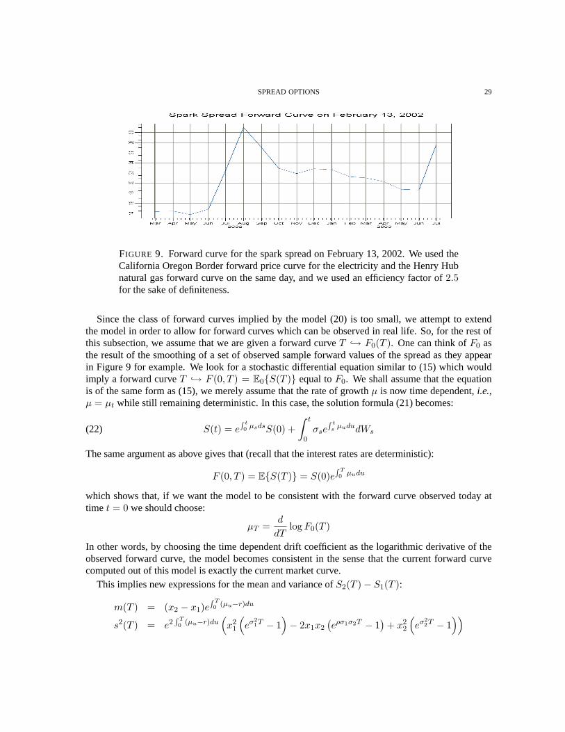
SPREAD OPTIONS 29

FIGURE 9. Forward curve for the spark spread on February 13, 2002. We used theCalifornia Oregon Border forward price curve for the electricity and the Henry Hubnatural gas forward curve on the same day, and we used an efficiency factor of2.5for the sake of definiteness.

Since the class of forward curves implied by the model (20) is too small, we attempt to extendthe model in order to allow for forward curves which can be observed in real life. So, for the rest ofthis subsection, we assume that we are given a forward curveT ↪→ F0(T ). One can think ofF0 asthe result of the smoothing of a set of observed sample forward values of the spread as they appearin Figure 9 for example. We look for a stochastic differential equation similar to (15) which wouldimply a forward curveT ↪→ F (0, T ) = E0{S(T )} equal toF0. We shall assume that the equationis of the same form as (15), we merely assume that the rate of growthµ is now time dependent,i.e.,µ = µt while still remaining deterministic. In this case, the solution formula (21) becomes:

(22) S(t) = e∫ t0 µsdsS(0) +

∫ t

0σse

∫ ts µududWs

The same argument as above gives that (recall that the interest rates are deterministic):

F (0, T ) = E{S(T )} = S(0)e∫ T0 µudu

which shows that, if we want the model to be consistent with the forward curve observed today attime t = 0 we should choose:

µT =d

dTlogF0(T )

In other words, by choosing the time dependent drift coefficient as the logarithmic derivative of theobserved forward curve, the model becomes consistent in the sense that the current forward curvecomputed out of this model is exactly the current market curve.

This implies new expressions for the mean and variance ofS2(T )− S1(T ):

m(T ) = (x2 − x1)e∫ T0 (µu−r)du

s2(T ) = e2∫ T0 (µu−r)du

(x2

1

(eσ

21T − 1

)− 2x1x2

(eρσ1σ2T − 1

)+ x2

2

(eσ

22T − 1

))


To be also consistent with our pricing formula (19) we therefore need take

σt =

√e2

∫ t0 µudu d

dt

(e−2

∫ t0 µudus2(t)

)as we have already derived.

The pricep of the spread option will still be given by formula (19) as long as we use the aboveexpressions for the constantsm(T ) ands(T ).

6. THE CASE K = 0, OR THE OPTION TO EXCHANGE

The textbook treatment of spread options is usually restricted to the special caseK = 0 becausewhen the distributions of the underlying indexesS1 andS2 are log-normal, this is the only case forwhich one has a solution in a closed forma la Black-Scholes for the price of the spread option withzero strike. This formula was first derived by Margrabe in [33] as early as in1978, and it bears hisname. We present this derivation in full for the sake of completeness, and because of its importance,we elaborate on some of its consequences.

6.1. Exchange of one Asset for Another.The caseK = 0 corresponds to anexchangesince thepay-off (S2(T ) − S1(T ))+ provides the holder of the option with the differenceS2(T ) − S1(T ) attimeT wheneverS2(T ) > S1(T ).

In order to illustrate this fact, let us assume that our business requires the purchase of one of thetwo products at timeT , that from a business point of view it does not make any difference which one,but that we have to decide at timet = 0 which one we will buy at timet = T . So let us choose theproduct whose price is given by the process{S2(t)}t and let us purchase the spread option at timet = 0. If the product we chose ends up being cheaper at timeT , we buy it at that time and we do notexercise the option, wasting the premium (i.e. the price we had to pay for the spread option.) On theother hand, if the product we chose ends up being more expensive at timeT , we buy it but we get theprice difference by exercising the option. So the spread option guarantees that pricewise, we will doas well as if we had chosen the cheapest one of the two at timeT . So having to cover the premium attime t = 0, may just be worth it.

6.2. Margrabe Formula. In this subsection we assume that the risk neutral dynamics of the twounderlying indexes are given by geometric Brownian motions, i.e. by stochastic differential equationsof the following form:

(23)dSi(t)Si(t)

= rdt+ σidWi(t) for i = 1, 2.

where the discount rater and the volatilitiesσi’s are constant. We assume that the two indexes are cor-related through the driving Brownian motions. To be more specific we assume thatE{dW1(t)dW2(t)} =ρdt. In other words,ρ is the parameter controlling the correlation between the two indexes.

Proposition 3. The pricep of a spread option with strikeK = 0 and maturityT , is given by:

(24) p = x2Φ(d1)− x1Φ(d0)

SPREAD OPTIONS 31

where:

(25) d1 =ln(x2/x1)σ√T

+12σ√T d0 =

ln(x2/x1)σ√T

− 12σ√T

and:

(26) x1 = S1(0), x2 = S2(0), σ2 = σ21 + σ2

2 − 2ρσ1σ2

Proof. In order to prove formula (24), we define two new independent Brownian motions{W1(t)}t

and{W2(t)}t by

dW2(t) = ρdW1(t) + ρ′dW2(t)

dW1(t) = dW1(t)

whereρ′2 + ρ2 = 1. dW1(t) anddW2(t) are well-defined as soon as|ρ| < 1. The risk-neutralvaluation rule gives us the price of a zero-exercise price spread option as follows

p = e−rT EQ{max(S2(T )− S1(T ), 0)}(27)

= e−rT EQ

{max

(S2(T )S1(T )

− 1, 0)S1(T )

}(28)

The price ofS2 expressed in the numeraireS1 (i.e. in units ofS1) remains a geometric Brownianmotion since:

d(S2(t)/S1(t))S2(t)/S1(t)

=dS2(t)S2(t)

− dS1(t)S1(t)

− cov

(dS2(t)S2(t)

− dS1(t)S1(t)

;dS1(t)S1(t)

)= (ρσ2 − σ1)dW1(t) + ρ′σ2dW2(t) + σ1(σ1 − ρσ2)dt

Using Girsanov’s theorem, we define a new probability measureP which Radon-Nikodym derivativewith respect toQ given on theσ-algebraFT by:

(29)dPdQ

∣∣∣∣FT

= exp(−1

2σ2

1T + σ1W1(T ))

UnderP, W1(t)− σ1t andW2(t) are Brownian motions. So:

p = e−rTS1(0)EP

{max

(S2(T )S1(T )

− 1, 0)

exp(

12σ2

1T − σ1W1(T ) +(r − 1

2σ2

1

)T + σ1W1(T )

)}= S1(0)EP

{max

(S2(T )S1(T )

− 1, 0)}

whereS2/S1 is geometric Brownian motion underP with volatility

(30) σ2 = σ21 + σ2

2 − 2ρσ1σ2

Using this fact, the last expression can be viewed as the price of a vanilla call option with no interestrate, strike 1 and volatilityσ2. The value is thus given by the classical Black-Scholes formula.

Remarks


1. The above result easily extends to allow for dividend payments at a constant rate. Suppose thatinstead of (23), we have

(31)dSi(t)Si(t)

= (r − qi)dt+ σidWi(t) for i = 1, 2.

The method remains the same as long as we useS1(t)eq1t andS2(t)eq2t in lieu ofS1(t) andS2(t). Inthat case, the price of a zero strike spread option is given by

p = x2e−q2T Φ(d1)− S1(0)e−q1T Φ(d0)(32)

d1 =ln(x2/x1)− (q2 − q1)T

σ√T

+12σ√T(33)

d0 =ln(x2/x1)− (q2 − q1)T

σ√T

− 12σ√T(34)

2. As [25] points out, it is interesting to note that these formulae are independent of the risk-freerater. This is because after risk adjustment (some would sayin a risk-neutral world), both underlyingindexes increase at the same discount rate, offsetting each other in the computation of the differenceappearing in the definition of the spread.

3. The above closed form formulae are very nice, but unfortunately, the case whereK 6= 0 cannotbe treated with the same success. Reviewing the approach outlined in Section 4 where we discussedthe use of multiple integrals, we can first condition byW1(T ) in (27). This gives:

(35) p = e−rT EQ{EQ{(S2(T )− S1(T )−K)+|W1(T )}

}The inner expectation can again be evaluated using the Black-Scholes formula with strikeS1(T )+Kand a slightly modified spot. But the outer expectation (the integration of the Black-Scholes formula)cannot be done explicitly.

7. PRICING OPTIONS ON THE SPREAD OF GEOMETRIC BROWNIAN M OTIONS

We continue our analysis of the valuation of spread options with non-zero strike prices. The resultsof the previous section apply when the dynamics of the underlying indexes (or the prices of theforward contracts on these indexes) are given by arithmetic Brownian motions. Now we consider thecase of the Samuelson’s model according to which these dynamics are given by geometric Brownianmotions. Since we are only considering options with European exercises in this paper, we need onlyto consider the distribution of the underlying indexes at a fixed time, and according to this model,the distribution of the spread is the distribution of the difference of two log-normal distributions.Unfortunately, except in the case of the exchange option (i.e., the spread option with strikeK = 0)considered in Section 6, the price of the spread option cannot be given by a formula in closed form,and as we already explained, this was the motivation for the introduction of the arithmetic Brownianmotion model. We now tackle the problem of the geometric Brownian motion.

Throughout this section we assume that, besides a riskless bank account with constant interest rater, our arbitrage-free market consists of two assets whose risk-neutral price dynamics are given by the

SPREAD OPTIONS 33

following stochastic differential equations:

dS1(t) = S1(t)[(r − q1)dt+ σ1dW1(t)]dS2(t) = S2(t)[(r − q2)dt+ σ2dW2(t)]

whereq1 andq2 are the instantaneous dividend yields, the volatilitiesσ1 andσ2 are positive constantsandW1 andW2 are two Brownian motions with correlationρ. The initial conditions will be denotedby S1(0) = x1 andS2(0) = x2. The discussion of this section focuses on the pricing of spreadoptions on twostocks.The case of spread options on two futures contracts follows immediately bytakingq1 = q2 = r.

The pricep of formula (8) can be rewritten in the form:

p = e−rT E{(

x2e(r−q2−σ2

2/2)T+σ2W2(T ) − x1e(r−q1−σ2

1/2)T+σ1W1(T ) −K)+}

which shows that the pricep is given by the integral of a function of two variables with respect to abivariate Gaussian distribution, namely the joint distribution ofW1(T ) andW2(T ). This expectationis of the form:

(36) Π = Π(α, β, γ, δ, κ, ρ) = E{(

αeβX1−β2/2 − γeδX2−δ2/2 − κ)+}

whereα, β, γ, δ andκ are real constants andX1 andX2 are jointly GaussianN(0, 1) randomvariables with correlationρ. These expectations were studied in [5]. We can therefore apply theresults of [5] to approximate the price of a spread option provided we set

α = x2e−q2T β = σ2

√T γ = x1e

−q1T δ = σ1

√T and κ = Ke−rT .

7.1. A Pricing Formula. The analysis of [5] is based on simple properties of the bivariate normaldistribution and elementary convexity inequalities. Combining the two, the authors derived a familyof upper and lower bounds for the pricep. Among other things, they show that the supremump oftheir lower bounds provides a very precise approximation to the exact pricep. Before we can statethe main result of [5], we introduce the notationθ∗ for the solution of the equation:

1δ cos θ

ln(− βκ sin(θ + φ)γ[β sin(θ + φ)− δ sin θ]

)− δ cos θ

2(37)

=1

β cos(θ + φ)ln(− δκ sin θα[β sin(θ + φ)− δ sin θ]

)− β cos(θ + φ)

2

where the angleφ is defined by settingρ = cosφ. The following proposition gives the closed formformula derived in [5] for the approximate pricep.

Proposition 4. Let us set:

d∗ =1

σ cos(θ∗ − ψ)√T

ln(x2e

−q2Tσ2 sin(θ∗ + φ)x1e−q1Tσ1 sin θ∗

)− 1

2(σ2 cos(θ∗ + φ) + σ1 cos θ∗)

√T

where the anglesφ andψ are chosen so that:

cosφ = ρ and cosψ =σ1 − ρσ2

σ.


Then

(38) p = x2e−q2T Φ

(d∗ + σ2 cos(θ∗ + φ)

√T)−x1e

−q1T Φ(d∗ + σ1 sin θ∗

√T)−Ke−rT Φ(d∗)

Note that this formula is as close to the Black-Scholes’ formula as we could hope for. Moreover,as documented in [5] it provided with extremely precise an approximation of the exact price of thespread option. One of the possible reasons for its accuracy is the fact that it gives exactly all knownparticular cases. Indeed, it has the following properties.

Proposition 5. The approximationp is equal to the true pricep whenK = 0, or x1 = 0, or x2 = 0,or ρ = −1. In particular, p is given by Margrabe’s formula whenK = 0, and by the classicalBlack-Scholes’ formula whenx1x2 = 0.

Proof. We refer to [5] for a complete proof. For the sake of completeness, we show how we recoverMargrabe’s formula in the caseK = 0. First we notice thatθ∗ is given by:

θ∗ = π + ψ = π + arccos(σ1 − ρσ2

σ

).

with:

σ =√σ2

1 − 2ρσ1σ2 + σ22

which implies that

σ2 sin(θ∗ + φ) = σ1 sin θ∗

and

d∗ =1

σ√T

ln(x2e

−q2T

x1e−q1T

)− 1

2(σ2 cos(θ∗ + φ) + σ1 cos θ∗)

√T .

Consequently:

σ2 cos(θ∗ + φ)− σ1 cos θ∗ = σ

and:

d∗ + σ2 cos(θ∗ + φ)√T =

1σ√T

ln(x2e

−q2T

x1e−q1T

)+σ√T

2

d∗ + σ1 cos θ∗√T =

1σ√T

ln(x2e

−q2T

x1e−q1T

)− σ

√T

2.

hold true. Finally, we have:

p = x2e−q2T Φ

(1

σ√T

ln(x2e

−q2T

x1e−q1T

)+σ√T

2

)− x1e

−q1T Φ

(1

σ√T

ln(x2e

−q2T

x1e−q1T

)− σ

√T

2

)which is exactly Margrabe’s formula.

SPREAD OPTIONS 35

7.2. Hedging and the Computation of the Greeks.In Subsection 4.4 we discussed some of theshortcomings of the existing numerical approximations to the price of a spread option. There weemphasized the importance of hedging, and we explained that most of the pricing algorithms did notaddress this issue, failing to provide efficient methods to evaluate the so-called Greeks. Following[5], we show that hedging strategies can be computed and implemented in a very efficient way usingformula (38) givingp.

We first consider the replication issue. The derivation of formula (38) cannot provide an exactreplication of the pay-off of the spread option. Because it is based on lower bounds, it gives a sub-hedge for the option.

Proposition 6. [5]The portfolio comprising at each timet ≤ T

∆1 = −e−q1T Φ(d∗ + σ1 cos θ∗

√T)

and

∆2 = e−q2T Φ(d∗ + σ2 cos(θ∗ + φ)

√T)

units of the underlying assets is a sub-hedge for the option in the sense that its value at the maturityof the option is almost surely a lower bound for the pay-off.

But as we mentioned earlier, beyond the first partial derivatives with respect to the initial valuesof the underlying assets which give the portfolio of the previous proposition, all the sensitivities ofthe price with respect to the various parameters are of crucial importance. The closed form formuladerived forp can be used to compute explicitly the other partial derivatives of the price. These are theso-called Greeks of the financial literature. We give some of them in the following proposition.

Proposition 7. [5] Letϑ1 andϑ2 denote the sensitivities of the price functional (38) with respect tothe volatilities of each asset,χ be the sensitivity with respect to their correlation parameterρ, κ bethe sensitivity with respect to the strike priceK andΘ be that with respect to the maturity timeT .

ϑ1 = x1e−q1Tϕ

(d∗ + σ1 cos θ∗

√T)

cos θ∗√T

ϑ2 = −x2e−q2Tϕ

(d∗ + σ2 cos(θ∗ + φ)

√T)

cos(θ∗ + φ)√T

χ = −x1e−q1Tϕ

(d∗ + σ1 cos θ∗

√T)σ1

sin θ∗

sinφ

√T

κ = −Φ (d∗) e−rT

Θ =σ1ϑ1 + σ2ϑ2

2T− q1x1∆1 − q2x2∆2 − rKκ

These formulae are of great practical value. The price of an option is determining factor for a buyerand a seller to get into a contract. But by indicating in which direction the price should change whensome of the parameters change, the partial derivatives are monitored by the investors, the traders andthe risk managers throughout the life of the option, i.e. up until maturity. The second order partialderivatives can also be approximated in the same way. We refrain from reproducing the results hereand we refer the interested reader to [5].


7.3. Comparison of the Three Approximations. We conclude this section with a short comparativeanalysis of the three approximation methods which we recommend for the actual pricing and hedgingof spread options.• Let us first compare the results of the Bachelier’s model with the results obtained with the approxi-mationp given by formula (8). Numerical experiments show that Bachelier’s price isalwayssmallerthanp, and this strongly supports the use ofp. Given the simplicity of the formulae provided by theBachelier’s approximation, the overhead caused by the used of formula (8) needs to be justified. Thisis quite easy since the latter only requires the numerical computation of the zero of a given function.This is done very efficiently by a Newton-Raphson method. The computation time is very small.• Let us now compare the approximation given byp with the results obtained using Kirk’s approx-imation. As we have already pointed out, the case in favor of the use ofp is mostly based on theeasy computations of the Greeks which in turn give sensible hedging portfolios. Since Kirk’s formulaalso leads to twodelta hedges,one can wonder how the performances of the two hedging strategiescompare along a given scenario.

To illustrate this point we reproduce a simulation study done in [5]. For a given scenario repre-senting a possible sample realization of the time evolution of the underlying assetsS1(t) andS2(t),we compare the payoff of the spread option at maturity with the terminal value of the portfolio ob-tained byn hedging operations throughout the life of the option. So for each scenario, we obtainthree tracking errors computed at maturity by trying to replicate the payoff of the option by the valueof portfolios obtained by re-balancing the portfolion times using thedelta hedgeprescriptions givenby the Bachelier’s method, Kirk’s formula and Proposition 6. To avoid an artificial dependence withrespect to a particular scenario, we repeat this operation for a large number of scenarios and we ac-tually compare the standard deviations of the tracking errors. The plots of Figure 10 where obtainedby varyingn from 1 to 1000 and with two different sets of parameters, but the results are prettygeneric. Indeed, we found that in most cases, the hedges provided by Proposition 6 and Kirk’s modelare equally very good, with in some cases a significant advantage for the former which seems to per-form much better in many cases. In any cases, these two models clearly out-perform the Bachelier’smodel. The reasons for this poor hedging performance of the Bachelier’s model are twofold. Firstly,the Bachelier’s model is based on a distribution assumption which stands the test of the pricing for-mula, but which cannot survive differentiation. Secondly, it is intrinsically a one-factor model tryingto directly model the distribution of the differenceS2(T )− S1(T ), and as such, it cannot capture thesubtle structure of the true nature of the two-factor model log-normal model we are dealing with.

7.4. Extension to Jump-Diffusion Models. The inclusion of a jump term in the stochastic differ-ential equations giving the dynamics of the underlying assets was proposed by Merton [35] and Coxand Ross [9] almost thirty years ago. Nevertheless these jump diffusion models remain at the levelof a scientific curiosity, mostly because of the difficulties associated with their statistical calibration.A renewal of interest in these models was prompted by the consequences of several severe marketcrashes and the extremely volatile behavior of the prices of new instruments such as electric powerfor example.

The approximation formula for the price of a spread option which we presented in this section caneasily be adjusted to apply to underlying asset price dynamics with jumps. At the risk of been sweptby the tidal wave of jump-diffusion processes introduced in the last ten years, we venture outside

SPREAD OPTIONS 37

FIGURE 10. Behavior of the tracking error as the number of re-hedging times in-creases. The model data arex1 = 100, x2 = 110, σ1 = 10%, σ2 = 15% andT = 1.ρ = 0.9,K = 30 (left) andρ = 0.6,K = 20 (right).

the class of continuous diffusion processes to prove our claim. The class of jump processes we areconsidering is often referred to as the Merton’s jump model in the financial literature. So, we allowfor jumps in the risk-neutral dynamics of the underlying assetsS1 andS2 by assuming that they aregiven by stochastic equations of the form:

(39)dSi(t)Si(t−)

= (r − qi − λiµi)dt+ σidWi(t) + (eJi(t) − 1)dNi(t)

whereN1 andN2 are two independent Poisson processes of intensityλ1 andλ2. They are alsoassumed to be independent ofW2 andW1. Finally, (J1(t))t≥0 and (J1(t))t≥0 are assumed to beindependent sequences of independent Gaussian random variablesN(mi, s

2i ). In the same way the

stochastic differential equation 13) giving the Samuelson’s dynamics could be solved to give theexplicit expressions (14) for the underlying assets, equation (39) can also be solved by a simple useof the extension of Ito’s formula for processes with jumps. We get the integrated price dynamics

Si(T ) = xi exp

(r − qi − σ2i /2− λiµi)T + σiWi(T ) +

Ni(T )∑k=1

Ji(k)

The expectation giving the pricep of a spread option can be computed by first conditioning withrespect to the Poisson processes, and in so doing, we reduce the problem to pricing spread optionsfor underlying assets with log-normal distributions. Indeed, givenN1(T ) andN2(T ), the randomvariablesS1(T ) andS2(T ) still have a log-normal distribution and the lower bound can be used. Thisleads to the following result.

Proposition 8. [5] If we setµi = emi+s2i /2 − 1 for i = 1, 2 and if we denote byp(x1, x2, σ1, σ2, ρ)

the price approximation given by (8), then the price of the spread option in the Merton’s model can


be approximated by the quantity:

(40) pjumps =∞∑i=0

∞∑j=0

e−(λ1+λ2)T (λ1T )i(λ2T )j

i!j!p (x1, x2, σ1, σ2, ρ)

with

x1 = x1e−λ1µ1T+i(m1+s2

1/2)

x2 = x2e−λ2µ2T+j(m2+s2

2/2)

σ1 =√σ2

1 + is21/T

σ2 =√σ2

2 + js22/T

ρ =ρσ1σ2√

σ21 + is21/T

√σ2

2 + js22/T

The above formula involves the summation of an infinite series. Its rate of convergence can be es-timated from a simple upper bound onp, and given any tolerance level, one easily determines howmany terms we need in (40) to satisfy the prescribe error bound.

8. EXTENSIONS AND GENERALIZATIONS TO ENERGY SPOT PRICES M ODELS

As in the case of the fixed income markets, commodity markets mathematical models come in twovarieties: either in the form of (finite) factor models, or models for the dynamics of the entire forwardcurve, as those we shall review in Section 9. This section is devoted to a short review of the simplestfactor models used in the industry, together with a discussion of the consequences of the assumptionsof these models on the price of spread options.

The simplest finite factor models are the one-factor models where the factor is chosen to be thecommodity spot price. So for the purpose of the present section, we can assume thatS1(t) andS2(t)are the spot prices at timet of two commodities. It is difficult to say whether or not the models usedin the previous sections are good for these indexesS1(t) andS2(t). Indeed, the stochastic differentialequations we used for the dynamics of the underlying indexes under a risk neutral measure. Indeed,these risk adjusted dynamics cannot be observed directly, and the best one can do is to calibrate thecoefficients of the models to the observed prices, which we did consistently when making sure thatour models could reproduce the observed forward curves.

In order to justify, or at least to motivate, the assumptions of the subsequent models, we take a shortexcursion in the real world of historical prices and of stochastic models for the historical dynamicsof spot prices. It is important to keep in mind that in most cases, Girsanov’s theory implies that thestochastic differential equations giving the historical dynamics differ from the risk adjusted modelsonly through the drift part.

The geometric Brownian motion models proposed by Samuelson for the time evolution of equityprices are appropriate for the dynamics of many assets, but they fail to capture one of the maincharacteristic feature of interest rates and physical commodity prices,mean reversion.This featureis included in the historical models by assuming that the dynamics of the underlying indexesSi(t)

SPREAD OPTIONS 39

are given by geometric Ornstein-Uhlenbeck processes instead of geometric Brownian motions. Theseprocesses can be defined as the solutions of stochastic differential equations of the form:

(41) dSi(t) = Si(t)[−λi(logSi(t)− αi)dt+ σidWi(t)]

where the constantsλi are positive. These constants are called themean reversioncoefficients. Theycan easily estimated from historical data. A simple linear regression can be used to do just that.See for example [7] for details and examples. Notice that the other parametersσi andαi can alsobe estimated very easily from historical data. Obviouslyσi is the volatility, and it can be estimatedempirically from the variance of the increments of the logarithms, whileαi is a simple functionof the of the asymptotic mean reversion level. Historical models are useful for risk management,and nowadays for an increasing number of pricing algorithms based on replication arguments andexpected utility maximization.

But the major issue is not the statistical estimation of the parameters of the historical model, thisis relatively easy. What we need in order to use the results of the theory presented in the first part ofthis paper, is a risk adjusted model. If we do not have any a-priori information on the risk premium,the drift of the risk adjusted dynamics can be absolutely anything. Indeed, it is easy to cook up a riskpremium process so that Girsanov’s theorem will turn the historical driftSi(t)[−λi(logSi(t)−αi)dtinto any prescribed drift. For this reason, it is common practice to specify the risk neutral dynamicsdirectly without trying to derive them from a Girsanov transformation on a model of the historicaldynamics appropriately fitted from empirical data. Then, it can be argued that since we want to beworking under the risk-neutral measure, the drift has to be equal to the risk free rate and changing itis pure non-sense. However, the risk-neutral drift determines the discounting factor used to determinepresent values of future cash flows, and as such it can be different from the short interest rate. Forexample, we included earlier the dividend rate in the risk neutral drift of dividend paying stocks. So inthe case of physical commodities, especially those commodities which cannot be stored like electricpower, the risk adjusted drift should not only encompass the dividend yield besides the risk free ratebut also some form of stochastic convenience yield (i.e., a stochastic dividend yield). Several recentstudies have given strong empirical evidence of the presence of a term structure of convenience yieldfor physical commodities. In particular, a form ofspot convenience yieldis often used as a factorjoining the commodity spot price in the list of factors driving the dynamics of the forward prices. Seefor example [36].

For the rest of this section we shall assume that the risk-neutral dynamics are specified by a meanreverting equation of the form (41). This practice can only be justified by assuming that the riskpremium is conspiring to preserve the mean reverting characteristic of the historical drift. Short ofmathematical convenience, we do not see on which ground to justify this assumption. Despite thisobvious lack of rationale, this assumption is nevertheless now widely accepted as reasonable in themathematical analysis of the dynamics of the commodity spot prices. See for example [7].

8.1. Adding Mean Reversion to the Models.We now assume that the risk neutral dynamics of theunderlying indexes are given by stochastic differential equations of the form

(42) dSi(t) = Si(t)[−λi(logSi(t)− µi)dt+ σidWi(t), i = 1, 2


where as before the volatilitiesσ1 andσ2 are positive constants, whereW1 andW2 are two Brownianmotions with correlationρ, whereλ1 > 0, λ2 > 0, and whereµ1 andµ2 are real constants. The pos-itive constantsλi give the rates of mean reversion. Indeed, as we are about to see, indexes satisfyingthese dynamical equations tend to revert toward the levelseµ

∞i if we setµ∞i = µi − σ2

i /2λi. Variousforms of equations (42) have been used as models for asset dynamics. For example, Schwartz [41]introduced them to derive closed form formulae for commodity contract prices.

Equations (42) can be best understood after a simple transformation leading to the dynamics of thelogarithms of the underlying indexes. SettingXi(t) = logSi(t), a simple application of Ito’s formulagives:

(43) dXi(t) = −λ[Xi(t)− µ∞i ]dt+ σidWi(t)], i = 1, 2

which shows that the logarithms of the indexes are nothing but classical Ornstein-Uhlenbeck pro-cesses whose mean reverting properties are well-known.

Even though equations (42) are more involved than the equations giving the dynamics of the geo-metric Brownian motions used in the previous sections, we can still derive explicit formulae for theindexesSi(T ) in terms of exponentials of correlated Gaussian variables. Indeed,Si(T ) = eXi(T )

with:

(44) Xi(T ) = µ∞i + e−λi(T−t)[Xi(t)− µ∞i ] + σi

∫ T

te−λi(T−s)dWi(s)

Hence:

(45) Si(T ) = eµ∞i +e−λiT (xi−µ∞i )+σi,T ξi

where

σi,T = σi

√1− e−2λiT

2λi, i = 1, 2

andξ1 andξ2 areN(0, 1) random variables with correlation coefficientρ given by:

ρ =1

σ1,Tσ2,TE{ξ1ξ2}

=1

σ1,Tσ2,TE{σ1

∫ T

0e−λ1(T−s)dW1(s)σ2

∫ T

0e−λ2(T−s)dW2(s)

}=

ρσ1σ2

σ1,Tσ2,T

1− e−(λ1+λ2)T

λ1 + λ2

= ρ

√λ1λ2

(λ1 + λ2)/21− e−(λ1+λ2)T

√1− e−2λ1T

√1− e−2λ2T

Consequently, the pricep of a spread with strikeK and maturityT on the difference between theunderlying indexesS1 andS2 whose dynamics are given by (42) is given by the formula:

p = e−rT E{(S2(T )− S1(T )−K)+} = Π(α, β, γ, δ, κ, ρ)

with

α = e−rT+µ∞2 +e−λ2T (x2−µ∞2 )−σ22,T /2 and β = σ2,T = σ2

√1− e−2λ2T

2λ2

SPREAD OPTIONS 41

γ = e−rT+µ∞1 +e−λ1T (x1−µ∞1 )−σ21,T /2 and δ = σ1,T = σ1

√1− e−2λ1T

2λ1

with ρ defined as above, andκ = Ke−rT .In particular, we can use our formula to find an excellent approximation to this price and an excel-

lent hedging portfolio.

Calibration and Consistency with the Forward Curves. As in the case of the Bachelier model, wecan try to generalize the above mean reverting models in order to make it consistent with observedforward curves. At least in principle, this should be done in exactly the same way. But as we are aboutto see, technical difficulties arise and the computations are more involved. Indeed, if we replace thedynamics of the spot prices by the same mean reverting equations with time dependent coefficients,we get the following stochastic differential equations (we drop the subscripti = 1, 2 since it isirrelevant in the present discussion)

dS(t) = S(t)[−λ(logS(t)− µt)dt+ σtdWt]

and the logarithmX(t) = logS(t) of the underlying index satisfies the equation:

dX(t) = −λ[X(t)− (µt −σ2

t

2λ)]dt+ σtdWt

which can be explicitly solved, giving:

Xt = µt −σ2

t

2λ+ e−λt[X0 − µ0 +

σ20

2λ]−∫ t

0e−λ(t−s)[µs −

σ2s

2λ]ds+

∫ t

0e−λ(t−s)σsdWs

and consequently, since as before:

F (0, T ) = E0{S(T )} = E0{eX(T )}we get the formula:

F (0, T ) = exp[µT −

σ2T

2λ+ e−λT

(X0 − µ0 +

σ20

2λ

)−∫ T

0e−λ(T−s)

(µs −

σ2s

2λ

)ds

+12

∫ T

0e−2λ(T−s)σ2

sds

]The problem is now to find, for each given forward curveT ↪→ F (0, T ), a functiont ↪→ µt and/or afunctiont ↪→ σt satisfying the above equality.

8.2. Introducing Jumps. If the models of the previous subsection can easily be argued to be appro-priate for most commodity spot prices, it will still fall short of adequate for electricity spot prices.Indeed the latter exhibit extreme volatility and introducing jumps in the model may appear as the bestway to include sudden and extreme departures from the mean reverting level. See nevertheless [2] foran alternative way to achieve the same thing with a continuous diffusion without jumps. At the riskof promoting the confusion with the historical and the risk adjusted dynamics, we refer the reader tothe right panel of Figure 1 where one can see that the sudden and extreme departures from the meando appear in the historical data. This figure illustrate that fact in the case of the Palo Verde electricpower spot prices. In order to accommodate the case of spread options involving electric power (spark


spreads are the typical examples), we allow for jumps in the risk-neutral dynamics ofS2. We assumethat:

dS2(t) = S2(t−)[(r − λµ)dt+ σ2dW2(t) + (eJt − 1)dN(t)

whereN is a Poisson process of intensityλ independent ofW2 andW1. (Jt)t≥0 is a sequence ofindependent Gaussian random variables(m, s2) andµ is function ofm ands2. This case is evensimpler than the one studied before. Pricing formula have therefore already been obtained.

8.3. Consistency with the Observed Forward Curves.As before in the case of the simpler geo-metric Brownian motion model, we first compute the analytic form of the forward curves, and wefind ways to adjust the coefficients of the model to match the theoretical curves carried by the modelto the empirical curves.

9. M ODELING THE DYNAMICS OF THE FORWARD CURVES

The spot price models considered in the previous sections are extremely popular because of theirintuitive appeal and because of their mathematical tractability. Indeed, modelling the dynamics ofthe spot prices seems like a reasonable thing to do, and the log-normal distribution is amenable toclosed form formulae for many of the simplest single commodity derivatives. Unfortunately, thesemodels are not always satisfactory. Indeed, given the spot price process{St}t≥0 of a commodity,the no-arbitrage priceF (t, T ) at timet of a forward contract with expiryT should be given by theformula:

(46) F (t, T ) = Et{ST }

where as before, we use the notationEt{ · } for the conditional expectation with respect to all theinformation available up to timet. The log-normal models and their generalizations of the previoussections are simple enough to allow for explicit formulae for the conditional expectations appearing inthe right hand side of (46), but unfortunately, the forward curvesT ↪→ F (t, T ) produced in this wayare very rarely consistent with the actual forward curves observed in practice, and the various fixeswhich we proposed in the previous sections are not satisfactory since they force us to re-calibrate themodel every day! This major shortcoming is at the core of the search for more sophisticated modelswhich could account for the observable features of the forward curves. Some of these models areconsidered in this section. The main departure from the previous approach is to model the dynamicsof the entire forward curve instead of modeling only the dynamics of its leftmost point. So we state astochastic differential equation (in fact a system of a continuum of such equations) for the dynamicsof the entire forward curve. In analogy with the HJM models of the fixed income markets we assumethat for each maturity dateT , the dynamics of the forward curves are given by:

(47)dF (t, T )F (t, T )

= µ(t, T )dt+n∑

k=1

σk(t, T )dWk(t) t ≤ T

whereW = (W1, . . . ,Wn) is an-dimensional standard Brownian motion, and where then volatili-tiesσk are deterministic functions of the current datet and the time-of-maturityT . Such a model iscalled ann-factor forward curve model. It has been described as desirable in the technical literature(see,e.g., Chapter 8 of the book [7]) though implementations in the commercial software packagesavailable for energy risk management are still at a rather primitive stage.

SPREAD OPTIONS 43

Whenever we work on pricing, hedging, or asset valuation (power plant, gas storage,. . . ), we needto assume that the dynamics have been adjusted for risk,i.e., we need to use risk-neutral probabilities.In that case we will need to setµ(t, T ) ≡ r, since it guarantees thatt ↪→ F (t, T ) is a martingale foreach fixedT when discounted. But when we work on risk management, the driftµ(t, T ) will need tobe calibrated to historical data.

An Explicit Solution. The coefficientsµ andσk being assumed deterministic, the dynamical equation(47) can be solved explicitly and we get:

(48) F (t, T ) = F (0, T ) exp

[∫ t

0

[µ(s, T )− 1

2

n∑k=1

σk(s, T )2]ds+

n∑k=1

∫ t

0σk(s, T )dWk(s)

]which shows that the forward prices have a log-normal distribution. More precisely, we have:

(49) F (t, T ) = αeβX−β2/2

for X ∼ N(0, 1) and

(50) α = F (0, T ) exp[∫ t

0µ(s, T )ds

], and β =

√√√√ n∑k=1

σk(s, T )2

Dynamics of the Spot Price. Since the spot price is the left hand point of the forward curve (i.e.,S(t) = F (t, t)) we can derive an explicit expression for the spot price from equation (48) above.

(51) S(t) = F (0, t) exp

[∫ t

0[µ(s, t)− 1

2

n∑k=1

σk(s, t)2]ds+n∑

k=1

∫ t

0σk(s, t)dWk(s)

]and differentiating both sides we get:

dS(t) = S(t)[(

1F (0, t)

∂F (0, t)∂t

+ µ(t, t) +∫ t

0

∂µ(s, t)∂t

ds− 12σS(t)2

−n∑

k=1

∫ t

0σk(s, t)

∂σk(s, t)∂t

ds+n∑

k=1

∫ t

0

∂σk(s, t)∂t

dWk(s)

)dt+

n∑k=1

σk(t, t)dWk(t)

]where we set:

(52) σS(t)2 =n∑

k=1

σk(t, t)2.

One deduce from equation (53) the fact that the instantaneous volatility of the spot price is given byσS(t). Consequently we have:

(53)dS(t)S(t)

=[∂ logF (0, t)

∂t+D(t)

]dt+

n∑k=1

σk(t, t)dWk(t)

where the drift termD(t) is given by:

D(t) = µ(t, t)− 12σS(t)2+

∫ t

0

∂µ(s, t)∂t

ds−n∑

k=1

∫ t

0σk(s, t)

∂σk(s, t)∂t

ds+n∑

k=1

∫ t

0

∂σk(s, t)∂t

dWk(s)


Remarks:1. In a risk-neutral setting, the drift appearing in formula (53) has a nice interpretation. The first term,i.e., the logarithmic derivative of the forward, can be interpreted as a discount rate (i.e., the runninginterest rate) while the termD(t) can be interpreted as a convenience yield which many researchersin the field tried to model directly in order to find no-arbitrage models consistent with the data.2. As emphasized in [7], this drift is most of the time not Markovian because of the presence ofthe stochastic integral which typically depends upon the entire past of the forward curve evolution.An exception is provided by the risk-neutral (i.e., µ(t, T ) ≡ r) one factor model (i.e., n = 1) withvolatility σ1(t, T ) = σe−λ(T−t). Indeed, in this special case, the dynamics of the spot prices are givenby (53) with drift:

D(t) = λ[logF (0, t)− logS(t)] +σ2

4(1− e−2λt)

which shows that the spot price dynamics are those of an Ornstein-Uhlenbeck process with timedependent mean reverting level defined by:

(54)dS(t)S(t)

= [µ(t)− λ logS(t)]dt+ σdW (t)

which is exactly the generalization considered in Subsection 8.1 to accommodate mean reversion.The point of this remark is to stress the fact that mean reversion of the spot price is closely related tothe exponential decay of the forward volatility for large times to maturity.

Changing Variables. During our discussion of the format of the data available to analysts, we made acase for the switch to the time-to-maturity variableτ as an alternative to the time-of-maturityT . Thischange of variable could deceivingly appear as a mere change of notation without much effect on theanalytic expression giving the dynamics of the forward curves. This is not the case, for computingderivatives with respect tot of the functiont ↪→ F (t, t + τ) for τ fixed, involves partial derivativesof F with respect to both of its variables sincet appears in both places. This is in contrast withcomputing the derivative with respect tot of t ↪→ F (t, T ) for T fixed which obviously only involvesthe first partial derivative ofF . To be more specific, if we set:

(55) F (t, τ) = F (t, t+ τ), µ(t, τ) = µ(t, t+ τ), and σk(t, τ) = σk(t, t+ τ),

then the dynamics (47) of the forward curve rewrites:

(56) dF (t, τ) = F (t, τ)

[(µ(t, τ) +

∂

∂τlog F (t, τ)

)dt+

n∑k=1

σk(t, τ)dWk(t)

], τ ≥ 0.

9.1. Calibration by Principal Component Analysis. We now present an application of a standarddata analysis technique to the calibration of forward energy curve models. Our goal is twofold: wetry to justify the assumptions behind the model (47) chosen for the dynamics of the forward curves,and at the same time we show how to identify and estimate theσk from actual historical market data.

Fundamental Assumption. The main assumption of this subsection concerns the actual form of thevolatility functionsσk. We shall assume that the latter are of the form:

(57) σk(t, T ) = σ(t)σk(T − t) = σ(t)σk(τ)

SPREAD OPTIONS 45

where the functionσ(t) of the single variablet will be determined shortly. Revisiting formula (52)giving the instantaneous volatility of the spot price in light of this new assumption we get:

(58) σS(t) = σ(0)σ(t)

provided we set:

σ(τ) =

√√√√ n∑k=1

σk(τ)2.

This shows that our assumption (57) implies that the functiont ↪→ σ(t) is up to a constant multiplica-tive factor, necessarily equal to the instantaneous volatility of the spot price. We shall use this remarkto estimateσ(t) from the data, for example by computing the standard deviation of the spot price in asliding window of30 days. The plot of the instantaneous standard deviation of the Henry Hub naturalgas spot price computed in this way is given in Figure 11.

FIGURE 11. Henry Hub natural gas instantaneous standard deviation computed in asliding window of length30 days.

The Rationale for the Use of PCA. For the purpose of the present discussion we fix times to maturityτ1, τ2, · · · , τN and we assume that on each given dayt, we have quoted forward prices for each of thetimes to maturityT1 = t + τ1, T2 = t + τ2, · · · , Tn = t + τN . This assumption may require a littlemassaging of the data which we explain in detail below. In any case, it is a reasonable starting pointfor the present discussion. According to the stochastic dynamics derived in (56), we have:

dF (t, τi)F (t, τi)

=(µ(t, τi) +

∂

∂τlog F (t, τi)

)dt+ σ(t)

n∑k=1

σk(τi)dWk(t) i = 1, . . . , N


We now define theN × n deterministic matrixF by F = [σk(τi)]i=1,··· ,N, k=1,··· ,n. We can assumewithout any loss of generality that then column vectorsσk( · ) for k = 1, . . . , n are orthonormalvectors ofRN . The goal of this subsection is to explain how we estimate these vectors from historicaldata. First, we derive the dynamics of the logarithm of the forward prices applying Ito’s formula:(59)

d log F (t, τi) =(µ(t, τi) +

∂

∂τilog F (t, τi)−

12σ(t)2σ(τi)2

)dt+σ(t)

n∑k=1

σk(τi)dWk(t), τ ≥ 0.

Next we compute the instantaneous variance/covariance matrix{M(t); t ≥ 0} defined by:

d[log(F ( · , τi)), log(F ( · , τj))]t = Mi,j(t)dt

From (59) we see that:

M(t) = σ(t)2(

n∑k=1

σk(τi)σk(τj)

)or equivalently that

M(t) = σ(t)2FF T .

Our interest in the above computation is the fact that it gives a clear strategy to extract the componentsof the matrixF from historical data. Indeed, after estimating the instantaneous spot volatilityσ(t) ina rolling window as we explained earlier, we can estimate the matrixFF T from historical data as theempirical autocovariance ofln(F (t, ·)−ln(F (t−1, ·)) after normalization byσ(t). Diagonalizing thisempirical variance/covariance matrix, identifying the principal components among the orthonormalbasis of eigenvectors to get the columns ofF is the purpose of classical principal component analysis.

So the gist of this derivation is that under the assumption (57), if one is willing tonormalizethelog returns of the forward contract prices by the instantaneous volatility of the spot price, then theinstantaneous autocovariance structure of the entire forward curve becomes time independent andhence, it can be estimated from the data. Moreover, diagonalizing this autocovariance matrix willprovide the functionσk(τ), and from their relative sizes, we will be able to decide how many docontribute significantly to the dynamics, effectively choosing the ordern of the model. This singularvalue decomposition of the covariance matrix and its interpretation are known as Principal ComponentAnalysis (PCA for short) and its relevance to the historical modeling of the dynamics of the forwardcurves has been recognized in the fixed income markets first, before being adopted in the analysis ofthe energy markets. See for example [32] and [7].

Remark: PCA is based on the estimation of a covariance matrix, and as long as statistical estimationgoes, some form of stationarity is needed to be able to base the estimates on time averages. In theapproach described above, the reduction to stationarity was done the transformation of the data pro-vided by the division byσ(t). Introducing the instantaneous spot volatility as a normalizing factor tocapture the seasonality of the data is not the only way to use the PCA as a calibration tool. Anotherapproach has been advocated by the scientists of Financial Engineering Associates (an energy soft-ware and consulting provider). They propose to bin the forward curves into12 groups according tothe month of the datet, and then to perform the PCA in each of these bins. Thisseasonal principalcomponent analysisas they call it more likely to capture the seasonality of the forward curves whenpresent. But at the same time, it reduces drastically the size of the data sets from which the covariancematrices are estimated. Not only does it restrict the length of the forward curves modeled in this way

SPREAD OPTIONS 47

(typically to 12 months) but it also creates serious difficulties in the assessment of the confidence inthe results. Indeed, the PCA involves the inversion and the diagonalization of the covariance matrixestimate, and these operations are notoriously erratic and non-robust, especially when the matrix ispoorly conditioned, which is the expected situation.

9.2. Pricing Calendar Spreads in this Framework. As we already explained, a calendar spreadis the simplest forms of spread option because it involves only one underlying commodity, the twounderlying indexes being the prices of two forward contracts with different maturities, sayT1 andT2.So using the same notation as before we have:

S1(t) = F (t, T1) and S2(t) = F (t, T2)

and since we consider only deterministic factors, these forward prices are log-normally distributedand we can use our pricing formula with the coefficientsα, β, γ, δ andρ given by

α = F (0, T1), β =

√√√√ n∑k=1

σk(s, T1)2 γ = F (0, T2), and δ =

√√√√ n∑k=1

σk(s, T2)2

according to (50). Recall thatµ ≡ 0 since we are using the risk-neutral dynamics of the forwardcurves for pricing purposes. On the other hand the correlation coefficient is given by:

ρ =1T

n∑k=1

∫ T

0σk(s, T1)σk(s, T2) ds

9.3. Pricing Spark Spreads in this Framework. The methodology of this subsection can be usedfor all the cross-commodity spreads discussed earlier in the text. For the purpose of illustration,we discuss the specific case of the spark spread options, for they provide a challenging example ofcross-commodity instrument. Their pricing is of great importance both for risk management and assetvaluation purposes. We proceed to price them in the framework introduced in this section. Becausewe are now dealing with two commodities, we need to adjust the notation: we choose to use thesubscripte for the forward prices, times to maturity, volatility functions,. . . pertaining to the electricpower, and the subscriptg for the quantities pertaining to natural gas.

Description of a Spark Spread Option. LetFe(t, Te) andFg(t, Tg) be the prices at timet of a forwardelectricity contract with time-of-maturityTe and a forward natural gas contract with time-of-maturityTg. For the purpose of this subsection, a crack spread option with maturity dateT is a contingentclaim maturing at timeT which pays the amount

(Fe(T, τe)−HFg(T, τg)−K)+ .

where the efficiencyH is a fixed conversion factor andK is the strike. Obviously we assume thatT < min{T1, T2}. The buyer of such an option may be the owner of a power plant that transformsgas into electricity and may want to protect himself against too low electricity prices and too high gasprices.


Joint Dynamics of the Commodities. In complete analogy with (47) we assume that the joint dynam-ics of the forward prices of the two commodities are given by equations of the form:

(60)

{dFe(t, T ) = Fe(t, T )[µe(t, T )dt+

∑nk=1 σe,k(t, T )dWk(t)

dFg(t, T ) = Fg(t, T )[µg(t, T )dt+∑n

k=1 σg,k(t, T )dWk(t)

Notice that each commodity has its own volatility factors, and that the correlation between the twodynamics is built into the fact that they share the same driving Brownian motion.

Fitting the Join Cross-Commodity Model. Without going into all the gory details of the implemen-tation, we give the general components of the fitting procedure.

We assume that on any given dayt we have electricity forward contract prices forN (e) times tomaturityτ (e)

1 < τ(e)2 , · · · < τ

(e)

N(e) , and respectively that we have natural gas forward contract prices for

N (g) times to maturityτ (g)1 < τ

(g)2 , · · · < τ

(g)

N(g) . As explained in our discussion of the empirical data

issues, typically we haveN (e) = 12 andN (g) = 36 and evenN (g) = 84 more recently. Assuming(57) for both the electricity and the natural gas forward volatilities and estimating the instantaneousvolatilities σ(e)(t) andσ(g)(t) of the electricity and gas spot prices in a rolling window of30 days,we can consider, for each dayt, theN = N (e) +N (g) dimensional random vectorX(t) defined by:

X(t) =

(

log Fe(t+1,τ(e)j )−log Fe(t,τ

(e)j )

σ(e)(t)

)j=1,··· ,N(e)(

log Fg(t+1,τ(g)j )−log Fg(t,τ

(g)j )

σ(g)(t)

)j=1,··· ,N(g)

Running the PCA algorithm on the historical samples of this random vectorX(t) will provide a smallnumbern of significant factors, and fork = 1, · · · , n, the firstN (e) coordinates of these factors willgive the electricity volatilitiesτ ↪→ σ

(e)k (τ) for k = 1, · · · , n, while the remainingN (g) coordinates

will give the gas volatilitiesτ ↪→ σ(g)k (τ).

Pricing a Spark Spread Option. Risk neutral pricing arguments imply that the price of the spark-spread option at timet is given by:

(61) pt = e−r(T−t)Et

{(Fe(T, Te)−HFg(T, Tg)−K)+

}This pricing formula is handled with the pricing algorithms developed in this paper because the distri-butions ofFe(T, τe) andFg(T, τg) will be log-normal under the pricing measure. Indeed, the pricesat timeT are given by our PCA-based model. So under a risk-neutral measure the prices become

Fe(T, Te) = Fe(0, Te) exp

[−1

2

n∑k=1

∫ T

0σe,k(s, Te)2ds+

n∑k=1

∫ T

0σe,k(s, Te)dWk(s)

]and:

Fg(T, Tg) = Fg(0, Tg) exp

[−1

2

n∑k=1

∫ T

0σg,k(s, Tg)2ds+

n∑k=1

∫ T

0σg,k(s, Tg)dWk(s)

]As explained above, the correlation between the two markets in built into the random driving factorsbecause we use the same Brownian motions to drive the stochastic differential equations (60) both

SPREAD OPTIONS 49

for electricity and gas. Consequently we can use our pricing algorithm withS1(t) = HFg(t, Tg) andS2(t) = Fe(t, Te) so that we need only to choose:

α = Fe(t, Te), and β =

√√√√ 1T

n∑k=1

∫ T

0σe,k(s, T )2 ds

for the first log-normal distribution,

γ = HFg(t, Te), and δ =

√√√√ 1T

n∑k=1

∫ T

0σe,k(s, T )2 ds

for the second one and

ρ =1T

∫ T

0

n∑k=1

σe,k(s, Te)σg,k(s, Tg)ds

for their correlation.

10. CONCLUSION

This review concentrates on the mathematics of the pricing and hedging of spread options. Thischoice was motivated by the utmost importance of these financial instruments, and the rich variety ofmathematical tools which have already been used in their analysis. We reviewed the results publishedon this subject in the economics, financial, business and mathematical literature, and we tried to shedsome light on the major issue of hedging and computing accuracy in approximation schemes. Ourgoal is to make the applied mathematical community aware of the slue of problems remaining to besolved.

In so doing, we devoted a good part of our efforts to the discussion of a new pricing paradigmintroduced recently by the authors. While giving an exhaustive review of the existing literature, wecompared the performance both from a numerical and an analytical points of view, of our algorithmagainst all the existing methods known to us.

We chose to illustrate the concepts and the numerical methods reviewed in this paper with examplesfrom the energy markets. In doing so, we ended up providing a rather thorough review of the maintechnical challenges of these markets. Indeed, we reviewed extensively a) the important features ofthe data available to the traders and analysts, b) the statistical models used to describe them and tobuild risk management systems, and c) the pricing models used to value the complex instruments ofthe energy markets. The latter are a fertile ground for mathematical investigations and we believedthat applied mathematicians will be well advised to pay more attention to their analysis.

The paper tried to prepare the reader for some of the challenges facing that part of the appliedmathematics community interested in the practical applications of financial mathematics. Naturalextensions of some of the results reviewed in this paper could lead to useful developments. Forexample, some of the numerical approximations presented here can clearly be generalized to the caseof an option on linear combinations of assets (basket options, rainbow options,. . .) or any linearcombination of prices of a single asset at different times (discrete-time average Asian option forexample.) Such extensions would provide efficient algorithms to compute prices and hedges forthese options; they are sorely needed. On another front, it is clear that some of the explicit formulae


reviewed in the text can be inverted. This allows for efficient computations of implied quantities suchas volatilities and correlations. From these implied volatilities and correlations, one should be ableto build more complex models (stochastic volatility and/or stochastic correlation, jumps,. . .) whichshould better fit the market reality. This would be a welcome development for it is still unclear whatthese implied quantities should be in the framework of spread options.

REFERENCES

[1] M. Arak, P. Fisher, L. Goodman and R. Daryanani (1987): The municipal-Treasury Futures Spread.The Journal ofFutures Markets,7, 355-371.

[2] M. Barlow (2002): A Diffusion Model for Electricity Spot Price.Finance??, ??-??.[3] T. J. Brennan, K. L. Palmer and S. A. Martinez (2002): Alternating Currents: Electricity Markets and Public Policiy.

RFF Press, Washington DC.[4] D. Brigo and F. Mercurio (2001): Interest Rate Models: Theory and Practice. Springer Verlag, New York N.Y.[5] R. Carmona and V. Durrleman (2003): Pricing and Hedging Spread Options in a Log-Normal Model.Working Paper,

Department of Operations Research and Financial Engingeering, Princeton University.[6] P. Carr and D. Madan (1999): Option valuation using the fast Fourier transform.The Journal of Computational

Finance2(4) 61-73.[7] L. Clewlow and C. Strickland (2000): Energy Derivatives: Pricing and Risk Management. Lacima Publications.[8] G. Cortazar and E. S. Schwartz (1994): The Valuation of Commodity Contingent Claims.The Journal of Derivatives,

1, no.427-39.[9] J.C. Cox and S.A. Ross (1976): The Valuation of Options for Alternative Stochastic Processes.Journal of Financial

Economics,4, 145-166.[10] J.C. Cox, J.E. Ingersoll Jr and S.A. Ross (1981): The Relation between Forward Prices and Futures Prices.Journal of

Financial Economics,9, 321-346.[11] M. H. A. Davis (1998): Two-factor log-normal tree.TMI Technical Note,Tokyo-Mitsubishi International, London.[12] M. Dempster and S. Hong (2000): Pricing spread options with the Fast Fourier Transform, First World Congress of

the Bachelier Finance Society, Paris.[13] S. Deng, B. Johnson and A. Sogomonian (2001): Exotic electricity options and the valuation of electricity generation

and transmission assets.Decision Support Systems,30, 383-392.[14] J. C. Easterwood and A. J. Senchack Jr (1986): Arbitrage Opportunities with T-Bills / T-Bonds Combinations.The

Journal of Futures Markets,6, 433-442.[15] S. Errera and S. L. Brown (1999): Fundamentals of Trading Energy Futures & Options. PennWell, Tulsa OK.[16] A. Eydeland and K. Wolyniec (2002): Energy and Power Risk Management: New Developments in Modeling, Pricing

and Hedging. John Wiley & Sons, New York, NY.[17] E. Fournie, J.M. Lasry, J. Lebuchoux and P.L. Lions (2001): Applications of Malliavin calculus to Monte Carlo

methods in finance II.Finance and Stochastics5, 201-236.[18] E. Fournie, J.M. Lasry, J. Lebuchoux, P.L. Lions and N. Touzi (1999): Applications of Malliavin calculus to Monte

Carlo methods in finance.Finance and Stochastics3, 391-412.[19] M. Garman (1992): Spread the Load, Risk, London.[20] R. Gibson and E. S. Schwartz (1990): Stochastic Convenience Yield and the Pricing of Oil Contingent Claims.Journal

of Finance,45, no.3959-976.[21] P. B. Girma and A. S. Paulson (1998): Seasonality in Petroleum Futures Spreads.The Journal of Futures Markets,18,

581-598.[22] P. B. Girma and A. S. Paulson (1999): Risk Arbitrage Opportunities in Petroleum Futures Spreads.The Journal of

Futures Markets,19, 931-955.[23] S. Heston (1993): A closed-form solution for options with stochastic volatility, with applications to bond and currency

options.Revue of Financial Studies.[24] J. E. Hilliard and J. Reiss (1998): Valuation of Commodity Futures and Options under Convenience Yields, Interest

Rates, and Jump Diffusion in the Spot.Journal of Financial and Quantitative Analysis,33 no.161-86.[25] J. Hull (2000): Futures, Options and Financial Derivatives. 6th ed.

SPREAD OPTIONS 51

[26] Intenational Energy Agency (2001): Competition in Electricity Markets. OECO-IEA.[27] R. Jarrow and A. Rudd (1982): Approximate option valuation for arbitrary stochastic processes.J. Financial Econom-

ics,10, 347-369.[28] R. L. Johnson, C. R. Zulauf, S.H. Irwin and M.E. Gerlow (1991): The Soy-bean Complex Spread: An Examination

of Market Efficiency from the Viewpoint of a Production Process.The Journal of Futures Markets,11, 25-37.[29] F. J. Jones (1991): Spreads: Tails, Turtles and All That.The Journal of Futures Markets,11, 565-596.[30] I. Karatzas and S. Shreve (2000): Mathematical Finance. Springer Verlag, New York, NY.[31] E. Kirk (1995): Correlation in the Energy Markets, in Managing Energy Price Risk. London: Risk Publications and

Enron.[32] R. Litterman and J. Scheinkman: Common factors affecting bond returns.J. of Fixed Income,1, 49-53.[33] W. Margrabe (1978): The value of an option to exchange one asset for another.The Journal of Finance, 33, 177-186.[34] A. Mbafeno (1997): Co-movement term structure and the valuation of energy spread options, in: M. Dempster and S.

Pliska (eds), Mathematics of Derivative Securities, Cambridge University Press.[35] R. Merton (1976): Option Pricing when Underlying Stock Returns are Discontinuous.Journal of Financial Econom-

ics,4, 125-144.[36] K.R. Miltersen and E.S. Schwartz (2000): Pricing of Options on Commidity Futures with Stochastic Term Structure

of Convenience Yields and Interest Rates.J. of Financial and Quantitative Analysis,,.[37] D. Pilipovic: Energy Risk: Valuing and Managing Energy Derivatives. Mc Graw Hill.[38] G. Poitras (1998): Spread Options, Exchange Options, and Arithmetic Brownian Motion.The Journal of Futures

Markets,18, 487-517.[39] R. Rebonato (2001): Volatility and Correlation in the pricing of Equity, FX and Interest-Rate Options. John Wiley &

Sons.[40] L. C. G. Rogers and Z. Shi (1995): The value of an Asian option.Journal of Applied Probability, 32, 1077-1088.[41] E. S. Schwartz (1997): The Stochastic Behavior of Commoditiy Prices: Implications for Pricing and Hedging.The

Journal of Finance,52(3), 923-973.[42] F. J. Sturm (1997): Trading Natural Gas: cash futures, options and swaps. PennWell Publ. Co. Tulsa, OA[43] S. Stoff (2002): Power System Economics: Designing Markets for Electricity. IEEE Press, John Wiley & Sons Inc.

Philadelphia, PA.[44] M. Wahab, R. Cohn and M. Lashgar (1994): The Gold-Silver Spread: Integration, Cointegration, Predictability and

Ex-Ante Arbitrage.The Journal of Futures Markets,14, 709-756.

DEPARTMENT OFOPERATIONSRESEARCH AND FINANCIAL ENGINGEERING, PRINCETON UNIVERSITY, PRINCE-TON, NJ 08544, ALSO WITH THE BENDHEIM CENTER FOR FINANCE AND THE APPLIED AND COMPUTATIONAL

MATHEMATICS PROGRAM.E-mail address: [email protected]

DEPARTMENT OFOPERATIONSRESEARCH AND FINANCIAL ENGINGEERING, PRINCETON UNIVERSITY, PRINCE-TON, NJ 08544.

E-mail address: [email protected]

pricing and hedging spread options · pricing and hedging spread options ... of electricity trading...

Documents