price discovery in emerging commodity markets: spot and ... · 79 price discovery in emerging...

79

Price Discovery in emerging commoDity markets: sPot anD Futures relationshiP in inDian commoDity

Futures market

Brajesh kumar ajay PanDey O.P. Jindal Global University IIM Ahmedabad

ABSTRACT

The price discovery role of the Indian commodity futures markets is investigated through return and volatility spillovers between spot and futures prices. For agricultural commodities, the price discovery takes place in both spot and futures markets. However, in the harvest period, when the futures trading volume is high, the futures market leads the spot market whereas in the lean period both markets jointly perform a price discovery. For the precious metals and energy commodities, the futures markets lead the price discovery role. In the case of industrial metals, LME spot prices (which are taken as spot prices for settlement by Indian exchanges) play a significant role in the price discovery process in the Indian market.

Keywords: Indian commodity futures markets, price discovery, return spillover, volatility spillover.

GELİŞEN EMTİA PİYASALARINDA FİYAT KEŞFİ: HİNDİSTAN VADELİ EMTİA İŞLEMLERİ PİYASASINDA SPOT VE VADELİ İŞLEMLER İLİŞKİSİ

ÖZETHindistan Vadeli Emtia Piyasaları’nın fiyat keşfindeki rolü, spot ve vadeli işlemlerin fiyatları arasındaki fiyat ve oynaklık yayılması (spillover)incelenerek araştırılmaktadır. Tarım ürünleri için, hem spot hem de vadeli işlemler piyasalarında fiyat keşfi olmaktadır. Vadeli alış satışların yüksek olduğu hasat zamanında, vadeli işlemler piyasası spot piyasalara öncülük ederken vadeli alış satışların zayıf olduğu dönemlerde her iki piyasa beraber fiyatları belirlemektedirler. Değerli metaller ve enerji piyasalarında ise, vadeli işlemler piyasası fiyat keşfinde öncülük etmektedir. Sınai metaller göz önüne alındığında ise, Hindistan piyasasındaki fiyat keşfinde, Londra Metal Borsası (LME) spot fiyatları (Hindistan borsaları tarafından uzlaşma için bu fiyatlar, spot fiyatlar olarak kabul edilirler) önemli bir rol oynamaktadırlar.

Anahtar kelimeler: Hindistan Vadeli Emtia İşlemleri Piyasası, fiyat keşfi, getiri yayılması, oynaklık yayılması.

Boğaziçi Journal Vol. 25, no. 1(2011), pp. 79-121.

* Brajesh Kumar is an Assistant Professor in Jindal Global Business School at O.P. Jindal Global University, Sonipat, Haryana-131001, India. E-mail: [email protected]

** Ajay Pandey is a Professor at Indian Institute of Management (IIM Ahmedabad), Ahmedabad, Gujarat-380015, India. E-mail: [email protected]

80

In the empirical financial economics literature, the question of whether the spot or the futures markets play a dominant role in the price discovery process has often been raised and investigated. Although the spot and futures markets of an asset are subject to the same information, the lead-lag relationship between spot and futures markets indicates whether there is unidirectional flow of information from the futures (spot) market to the spot (futures) market or a bidirectional flow of information between these markets. The lead-lag relationship between spot and futures shows how fast one market reflects the new information vis-à-vis another and how well they are connected. In other words, it helps in understanding the strength of linkages between these markets and the speed of adjustments.

One of the important functions of futures markets is price discovery. To perform this function effectively, the futures markets are supposed to incorporate new information more quickly than the spot markets. Futures markets are supposed to lead spot markets given low transaction costs and lack of short-sale restrictions (Tse, 1999). Another interesting perspective in understanding spot-futures relationships originates from the efficient market hypothesis which says that all markets (spot/futures) should incorporate any new information simultaneously and they should not show any lead-lag relationship. However frictions in the markets, in terms of transaction costs and information asymmetry, can lead to return and volatility spillovers across markets. Studies on equity and commodity derivatives markets of developed markets have shown that the futures prices play a dominant role in price discovery. In the emerging markets, this issue has not been adequately researched, and limited studies report mixed results.

The characteristics of emerging markets are very different from that of developed markets. According to Bakaert and Harvey (1997) and Antoniou and Ergul (1997), emerging markets are characterized by low liquidity, thin trading volume, higher sample average returns, low correlation with developed market returns, non-normality, better predictability, higher volatility of returns, and small-size sample availability. It is usual to assume that the emerging futures markets exhibit higher price variability and poor information processing capabilities (Tomek, 1980; Carter, 1989). Poor flow of information may consequently affect the price discovery process in such markets. New commodity futures markets in developing economies like India usually have thin volumes and low market depth, lack of well developed spot markets, poor delivery systems, policy restrictions and taxes on the movement of commodities, and other market imperfections. Given these differences, it is important to investigate empirically the Indian commodity futures markets more extensively so as to shed light on the role played by the futures markets in the price discovery process.

Since the inception of the organized commodity derivatives markets in India in 2003, Indian futures markets have grown rapidly. In the year 2003, three national level multi-commodity exchanges, namely the National Multi Commodity Exchange (NMCE), the Multi Commodity Exchange (MCX) and the National Commodities and Derivatives Exchange (NCDEX), were set up. At present commodity futures are traded on these three national exchanges, and on 20 other regional exchanges. The futures contracts of around 103 commodities are traded on the three national exchanges. In terms of volume, Copper, Gold, Silver and Crude futures contracts traded on the Multi-Commodity Exchange (MCX) are ranked within the top 10 most actively traded futures contract(1) in the world. Despite phenomenal growth, the commodity futures markets in India are subject to many regulations, and many times the futures trading have been banned and criticized in the popular press and by the policy makers for speculative trading activity and for increasing the spot/price volatility.

81

Most of the studies on Indian commodity futures markets are on policy issues. Some of the major issues investigated and analyzed in this context are such things as the role of commodity spot markets integration and friction (high transaction costs) in these spot markets, proper futures contract design, identification of delivery location, importance of warehousing facilities and policy issues like restriction on cross-border movement of commodities, and different kind of taxes (Thomas, 2003; Kolamkar, 2004; and Nair, 2004). The studies on price discovery effectiveness of Indian commodities have been limited to regional exchanges, for a few commodities and with small samples from the period prior to setting up the national exchanges (Thomas and Karande, 2001; Sahadeven, 2002; and Naik and Jain, 2002). The Indian commodity futures markets have since matured, if increased trading volume is any indicator. The lead-lag relationship in returns and volatility between spot and futures markets has also not been explored extensively by the earlier studies on Indian commodity markets.

In order to fill the research gap, this paper investigates the return and volatility spillover between spot and futures markets for eleven commodities including agricultural commodities (Soybean, Corn, Castor Seed and Guar Seed), industrial metals (Aluminum, Copper and Zinc), precious metals (Gold and Silver) and energy commodities (Crude Oil and Natural Gas). In this paper, we examine the lead-lag relationship between spot and futures markets by examining the following questions: (a) do futures and spot prices share a long-term equilibrium relationship?; (b) do futures returns (volatility) lead the spot returns (volatility) in short and long-run?; and (c) if yes, is this relationship the same for different commodities which are different in terms of trading volume and tradability? Another important aspect of investigation is to understand the difference between the role of local spot markets and international spot markets in the price discovery process. In the case of agricultural commodities and precious metals, Indian spot markets are well developed and local spot prices are used, whereas for industrial metals and energy commodities, spot prices of international markets converted into Indian currency are used by Indian commodity futures exchanges. For industrial metals and energy commodities, spot markets in India are not well developed and local spot prices quoted by some producers or buyers of these commodities are a reflection of international prices, exchange and freight charges. This is the reason why National Commodity exchanges report international spot prices converted into Indian currency as spot prices. The return and volatility spillovers between spot and futures markets are examined through a Vector Error Correction (VECM)/Vector Autoregressive (VAR) model and Granger causality test. For modeling volatility spillover, following Schwert (1990), the absolute value of the residuals obtained from the conditional return VECM/VAR model are multiplied by (p/2)1/2 and are used as a proxy of volatility.

The rest of the paper is organized as follows: Section 2 briefly reviews studies on the lead-lag relationship in returns and the volatility in commodity futures markets. Section 3 outlines the data and the methodology used in the study. Empirical results are presented in Section 4. Section 5 summarizes the results and gives the conclusion.

LEAD-LAG RELATIONSHIP BETWEEN FUTURES AND SPOT MARKETS

The issue of the lead-lag relationship in returns and volatility in developed equity, currency and commodity markets has been extensively addressed and researched for a long time. The early research focused mostly on the price or return spillover effects between futures and spot markets. Recently the emphasis has shifted to how information is transmitted through volatility. In equity markets, there are numerous studies which explain the return and volatility spillovers between spot and futures markets.

82

Of late, studies in this area use high frequency (intraday) data to understand the relationship more precisely. Some of the important studies include the work of Gardbade and Silber (1983), Herbst, McCormack and West (1987), Kawaller et al. (1987), Stoll and Whaley (1990), Cheung and Ng (1990), Chan, Chan, and Karolyi (1991), Schroeder and Goodwin (1991), Chan (1992), Chang et al. (1995), Pizzi et al. (1998), Antoniou and Garrett (1993), Abhyankar (1998), Antoniou et al. (2001), Brooks et al. (2001), Hodgson, Masih, and Masih (2006), Floros and Vougas (2007), and Kavussanos, Visvikis and Alexakis (2008). In most of the studies, it was found that the futures markets lead the price discovery process. In this section, we review some of the important studies.

In commodity futures markets, Gardbade and Silber (1983) developed a model of price discovery in which changes in futures and spot prices at time t are modeled as a function of the basis at time t-1. They used daily spot and futures prices for four storable agricultural commodities (wheat, corn, oats and orange juice) to understand the price discovery process in storable agricultural commodities. For wheat, corn and orange juice, they found that the futures markets dominate the spot markets, but for oats the results were not clear enough. Following the same approach, Oellermann et al. (1989) and Schroeder and Goodwin (1991) studied the price discovery for livestock contracts and found that the futures markets capture the information first and then transfer it to the spot markets. Yang et al. (2001) examined the price discovery performance of the futures markets for storable (corn, oats, soybean, wheat, cotton, and pork bellies) and non-storable (hogs, live cattle, feeder cattle) commodities. They used cointegration procedures and vector error correction models (VECM) and found that the storability does not affect the price discovery process, and, for both storable and non-storable commodities, futures markets lead the spot markets.

Empirical research on the price discovery role of futures in emerging markets is relatively sparse. Brockman and Tse (1995) investigated the price discovery in the newly created Canadian commodity futures market using cointegration, VECM and the Hasbrouck (1995) information model. They investigated the lead-lag relationship between spot and futures prices in four agricultural commodities (canola, barley, oats, and wheat) and found that for all four commodities, the futures market leads the spot market and hence the price discovery was mainly driven by the futures market. Fortenberry and Zapata (1997) examined the lead-lag relationship between newly created futures and spot markets in the US for cheddar cheese, diammonium phosphate and anhydrous ammonia by using cointegration techniques. They found the evidence that futures and spot prices of diammonium phosphate and anhydrous ammonia markets are cointegrated but not that of cheddar cheese. Maynard et al. (2001) evaluated the performance of the thinly traded shrimp futures contracts traded on the Minneapolis Grain Exchange. They used weekly data of thirteen varieties of shrimp in the spot markets and two varieties in the futures markets and found that only one variety in the spot market was cointegrated with one of the futures contracts. All the other varieties in the spot markets were not cointegrated with any of the futures prices. Short-run analysis using Sims’ two-sided distributed lag model provided the evidence of weak relationships between spot and futures prices. Mattos and Garcia (2004) analyzed the relationship between spot and futures prices in the Brazilian agricultural markets and investigated the effect of trading activity on the price discovery of futures markets. They used daily data on Brazilian futures and spot prices of coffee (arabica), corn, cotton, live cattle, soybeans, and sugar and found mixed results. It was found that in the live cattle and the coffee markets, which have a higher trading volume, the futures and the spot prices were cointegrated. On the other hand, in thinly traded markets (i.e., corn, cotton, soybeans), no long-run relationship existed, and the short-run interactions were simultaneous and weak. They concluded that the price discovery process between spot and futures

83

prices is linked with the trading activity (liquidity) in the markets. Azizan et al. (2007) investigated the return and volatility spillovers in the Malaysian futures using bivariate ARMA(p,q)-EGARCH(p,q) model specifications. They used daily price data of crude palm oil futures and spot markets and found bidirectional information transmission between futures and spot markets for both returns and volatility.

In Indian commodity futures markets, very few studies have been done which are specifically related to return and volatility spillover between spot and futures markets. As mentioned earlier, most of the studies are limited to policy issues related to the development of the derivatives market. Thomas (2003) emphasized the importance of price transparency, institutional setup, cash settlement and dematerialized warehouse receipts for the development of the futures market in India. Kolamkar (2004) pointed out that the lack of awareness about the role and technique of futures trading among the potential beneficiaries, the absence of initial critical liquidity or high transactional costs, fragmented spot markets, excessive regulations in the commodity spot and futures markets, restrictions on holding of stocks, turnover, and movement of goods, bad quality of storage and warehousing are the major hindering blocks in the development of commodity futures markets in India. Nair (2004) advocated the importance of spot markets and certified warehouses in the development of commodity futures markets in India. Fragmented spot markets, various taxes and restriction on the free movement of commodities have been identified as major stumbling blocks for the development of commodity futures markets in India. The empirical research related to Indian futures markets is limited. Thomas and Karande (2001) studied the price discovery process in the castor seed futures market traded on Ahmedabad and Mumbai regional exchanges using the Gardbade and Silber (1983) model. They found that Ahmedabad and Mumbai markets react differently to information in the price discovery of castor seed. In the Bombay market, futures prices dominated the spot prices; however, no clear cut lead-lag between spot and futures prices was found in the Ahmedabad market. In the Ahmedabad market, which is the production center, it was found that in the harvest period, spot prices lead the futures prices. Sahadeven (2002) studied six commodities traded on 12 regional commodity exchanges to investigate the relationship between returns, trading volume, market depth, and volatility. He found that futures and spot markets are not integrated and trading volume and market depths are not significantly influenced by returns and volatility of spot and futures markets. He observed that the lack of efficient and modern infrastructure facilities, existence of the gray market and lack of participation in the futures markets are some of the relevant bottlenecks in the growth of futures markets in India. Naik and Jain (2002) studied the performance of six commodities on regional exchanges and concluded that the regional exchanges are not efficient in price discovery and risk management. They asserted that, “Barring a few, they [futures markets] are still not congenial markets for hedgers.” They found that the commodity futures markets are deficient in several aspects such as infrastructure, logistics, management, linkages with financial institutions, reliability and integrity, dominance of speculators, and inefficient information systems, which discourage market players from trading in futures markets. Roy and Kumar (2007) studied the market integration among wheat spot markets and the effect of wheat futures trading on spot market integration by using the Johansen cointegration test. They also investigated the lead-lag relationship between spot and futures prices by using the Garbade-Silber (1983) model, efficiency of futures markets using the Fama and French (1987,1988) model, and hedging effectiveness by using the OLS technique. It was found that the cointegration across spot markets had increased after the introduction of the futures market. Lead-lag relationship between spot and futures markets was mixed and wheat futures contracts had low hedging effectiveness. In the Indian context, most of the cited studies either had serious methodological limitations or were carried out on the data from regional exchanges which were less liquid in the absence of an electronic trading platform. Since the inception

84

of three national exchanges in 2003, the accessibility and hence the trading in futures contracts has increased many times. In the context of these exchanges, there is a need to investigate the linkage between spot and futures markets afresh.

To sum up, the studies on price discovery in developed markets tend to show that futures prices play a major role in the price discovery process. However, in emerging markets, results have been mixed. Empirical evidences also show that thinly traded contracts fail to provide an effective price discovery mechanism. In this paper, we investigate the lead-lag relationship in returns and volatility of futures and spot prices of Indian commodity futures markets during the period beginning in 2004 after which futures trading in India has increased considerably.

DATA SET AND METHODOLOGY

The lead-lag relationship in returns and volatility between futures and spot prices in this study is examined for four agricultural commodities (Soybean, Maize, Castor Seed, and Guar Seed), three industrial metals (Aluminum, Copper and Zinc), two precious metals (Gold and Silver), and two energy commodities (Crude Oil and Natural Gas). We analyze the near-month contracts and next-to-near-month contracts for which the trading volume is relatively high. We prepare the near-month futures time series and next-to-near-month futures time series on a rolling basis. That is, when the near contract approaches maturity, we select data from the next maturing contract. We also remove the maturity week data from the near-month futures series to remove the maturity bias. Futures contracts from the NCDEX are used for agricultural commodities (Soybean, Maize, Castor Seed and Guar Seed), and futures traded on the MCX are used for non-agricultural commodities. The selection of the exchange for selecting the futures contract is based on the trading volume of the commodity futures contracts on an exchange. All three national exchanges provide the daily closing price of all futures contracts. These exchanges also report the data of spot prices of these commodities. In the case of agricultural commodities, spot prices of local markets, which are production centers (Table 1), are reported. For precious metals, spot prices of Ahmedabad markets are used. In absence of developed spot markets for industrial metals, LME cash prices and for Crude Oil and Natural Gas, the NYMEX cash prices converted into Indian currency are reported on these exchanges. Details of the data period and the source of data are given in Table 1.

Table 1Details of Commodity, Data Period and Source

Commodity Data-Period Futures Market Spot Market

Agricultural

Soybean 09/01/2004 to 10/20/2008 NCDEX Indore Maize 01/05/2005 to 10/20/2008 NCDEX Nizamabad

Castor Seed 09/21/2004 to 10/20/2008 NCDEX Disa

Guar Seed 04/12/2004 to 09/19/2008 NCDEX Jodhapur

PreciousMetals

Gold 05/02/2005 to 09/30/2008 MCX Ahmedabad

Silver 05/02/2005 to 09/30/2008 MCX Ahmedabad

IndustrialMetals

Aluminum 02/01/2006 to 09/30/2008 MCX LME Cash Price

Copper 07/04/2005 to 11/20/2008 MCX LME Cash Price

Zinc 04/03/2006 to 09/30/2008 MCX LME Cash Price

EnergyCrude Oil 05/02/2005 to 09/30/2008 MCX NYMEX Cash PriceNatural Gas 07/21/2006 to 09/30/2008 MCX NYMEX Cash Price

85

We also divide the data into two non-overlapping sub-periods of almost two years each. The first sub-period from the years 2004 to 2006 represents the early phase of the national commodity exchanges and is characterized by a low futures trading volume and market depth; the second sub-period from year 2007 to 2008 is characterized by a relatively high futures trading volume and high market depth. The basic return characteristics of near-month futures, next-to-near-month futures and spot returns of the entire period and two sub-periods are estimated.(2) During the entire period, the mean spot returns are negative for all commodities except industrial metals. The futures volatility (standard deviation) in the first sub-period is higher than the second sub-period for most of the commodities. The near-month futures volatility is higher than next-to-near-month futures volatility for non-agricultural commodities. The spot volatility is higher than futures volatility for most of the commodities in the entire period as well as in the two sub-periods.

To examine the lead-lag relationship between spot and futures prices, we use either the VECM or the VAR model. If spot and futures prices are cointegrated, a VECM model is applied; otherwise, the VAR model is used. The volatility spillover is estimated through the VAR model in which spot and futures volatility are obtained from the absolute value of the residuals from the conditional returns (VECM/VAR) model and multiplied by (p/2)1/2 (Schwert, 1990).

Return Spillover: Vector Error Correction Model (VECM)

After identifying the cointegration between spot and futures prices, the short run dynamics between these markets is modeled using the VECM/VAR model. When futures and spot prices are cointegrated, return dynamics of the both prices can be modeled using a VECM model. VECM model specifications allow a long-run equilibrium error correction in prices in the conditional mean equations (Engle and Granger, 1987). A similar approach has been used to model the short run relationship of cointegrated variables (Harris et al., 1995; Cheung and Fung, 1997; Ghosh, Saidi and Johnson, 1999). If the futures and spot series are co-integrated in the order of one, then the Vector error correction model of the series is given by these equations:

(1)

In these, PS,t

and RS,t

is the log spot price and spot returns are calculated as the successive log price difference (P

S,t-P

S,t-1) respectively. Similarly, P

F,t and R

F,t is the log futures price and futures returns

respectively. The error correction term or (P =αβ’ representation) represents the speed of adjustment of returns towards long run equilibrium. The short run parameter estimates χ

F, χ

S, γ

F and γ

S measure the short run integration or return spillover.

The significance and value of these parameters measure the nature of short run spillover between these markets. If futures and spot prices are not cointegrated, then we use a VAR model. The VAR model specification is similar to the VECM model except for the error correcting terms.

86

Volatility Spillover: Vector Autoregressive Model (VAR)

Chan, Chan and Karolyi (1991) and Ross (1989) explained the importance of the information-volatility relationship and argued that the volatility is related to the amount of information released. Hence volatility is an important source of information apart from asset prices themselves. Following Schwert (1989, 1990) and Min and Najand (1999), the residuals from the VECM/VAR models of conditional returns are used as a proxy of the return volatility. The absolute values of residuals are multiplied by (p/2)1/2 to estimate the daily spot or futures volatility. The volatility spillover between spot and futures prices is investigated through a VAR model as represented by equation 2.

(2)

Here and V represent volatility. The residuals εF,t

and ε

S,t are the residuals obtained from the conditional mean equation of futures and spots respectively.

We apply the Granger Causality test to find the lead-lag relationship in volatility between spot and futures prices.

RESULTS AND DISCUSSION

The Lead-Lag Relationship between Spot and Futures Returns

The unit root in the price and return series is tested by the Augmented Dickey-Fuller (ADF, 1981) unit root test and it is found that all futures price time series are I(1) except the Soybean near-month series and next-to-near-month series in the first sub-period and the Guar Seed near-month futures series in the first sub-period and next-to-near-month futures series in the entire period and in the first sub-period. In the early phase of the Indian commodity futures market, which had very little futures trading volume, Soybean and Guar Seed futures prices violated the weak form of efficiency. This may be because of thin volumes, less participation of informed traders, excessive speculation or noise trading. The spot prices of all commodities except Soybean and Guar Seed in the first sub-period are I(1) series. After identifying the I(1) series, the Johansen Cointegration test is performed. The Johansen full information multivariate cointegrating procedure, which uses the vector error correction model (Johansen, 1988; and Johansen and Juselius, 1990), is widely used to perform the cointegration analysis. It can only be performed between the series with the same degree of integration. The lag length of the VECM model is identified through a minimum AIC criteria. We applied both the Trace Statistics, λ

trace and the Maximum Eigen value statistic, λ

max to find the cointegration between spot and

futures prices of I(1) series.

Results of the cointegration test between near-month futures and spot prices and next-to-near-month futures and spot prices are given in the Appendix. Both λ

trace and λ

max statistics indicate that the spot

and near month futures prices and the spot and next to near month futures prices of all commodities are cointegrated in the entire period as well as in both the sub-periods except for some commodities

87

in a particular period, as discussed later. In the case of near-month futures, where trading volume is relatively high, Guar Seed futures prices in the second sub-period are not cointegrated with the spot prices. This may be because of noise trading in the futures market or frictions in the spot market including possibly high transaction costs. Next-to-near-month futures prices of Natural Gas (in the entire period and both the sub-periods), Maize, Aluminum, and Copper (in the first sub-period), and Castor Seed and Crude Oil (in the second sub-period) are also not cointegrated with spot prices. As spot and futures prices are derived from the same underlying, they should be cointegrated with a common stochastic term. In case of the next-to-near month futures in the first sub-period (early stage of the Indian futures markets), the cointegration relationship is violated for 6 out of 11 commodities. The reason may be lack of volume in futures trading and less participation of informed trades in the early stage of the futures markets. However, in the recent period (second sub-period) in only 3 out of 11 commodities, the cointegration relationship between the next-to-near-month futures prices and spot prices is violated. These three commodities include two globally traded energy commodities -- Crude Oil and Natural Gas, which have shown a dramatic price movement in the recent period. It is interesting to note that in the recent period, the Indian commodity futures markets are linked with LME cash prices of the industrial metals but not with the NYMEX cash prices of the energy commodities. The other commodity is Castor Seed, where in the recent period spot and futures prices are not cointegrated. Again, it is found that the trading volume and open interest in the Castor futures markets has decreased dramatically in the recent sub-period. Our results on cointegration between spot and futures markets support the findings of Mattos and Garcia (2004) who investigated the same for Brazilian commodity futures markets and found that the spot and futures market are cointegrated for commodities where trading volume is high. In the case of thinly traded futures, neither long-run nor short-run interaction between spot and futures market was found.

After identifying the cointegration between spot and futures prices, the short run dynamics between these markets is modeled using the VECM/VAR model. Results of the VECM/VAR model are presented in the Appendix.

We find that in the case of the near-month futures, error correcting terms (γF,EC

and χ

S,EC) in the spot

returns are significant at a 5% level for all commodities. However, in futures the error correcting terms (χ

F,EC and

γ

S,EC) are significant for Soybean, Castor Seed, Guar Seed, Silver and Aluminum only.

In the next-to-near-month futures, other than these commodities, Copper futures returns also have a significant error correcting term. This indicates the joint role of spot and futures markets in long-run price discovery for agricultural commodities, Silver, Aluminum and Copper. The leading role of spot or futures markets in the long-run price discovery process is further investigated through a weak exogeneity test. The results of the VECM/VAR model also indicate that in most of the commodities, spot returns are autoregressive in nature and lagged parameters of spot returns are significant up to lag 4. The spot returns are also influenced by lagged futures returns. The autoregressive nature of spot returns and the effect of lagged futures returns is observed more in the case of agricultural commodities. Similar results are found for both the sub-periods.

The weak exogeneity test measures the speed of adjustment of prices towards the long run equilibrium relationship. If the two price series are cointegrated in the long-run, the weak exogeneity test measures the speed of adjustment of prices towards the long-run equilibrium. In the context of spot and futures markets, a weakly exogenous variable is the leading variable and the other variable adjusts to any disequilibrium in the long-run equilibrium relationship between the two. In the price discovery process,

88

a weakly exogenous variable assimilates new information first and then the other variable adjusts itself to the new information. The null hypothesis for the weak exogeneity test is that the prices are weakly exogenous and the test yields a Chi-square distribution. The results of the weakly exogenous test are reported in Table 2.

Table 2 Results of Weak Exogeneity Test

This table provides results of weak exogeneity test which measures the speed of adjustment of prices towards the long run equilibrium relationship between spot and futures prices. In this test null of weak exogeneity is tested against no exogeneity.(a) Near Month Futures Prices and Spot Prices

2004-2008 2004-2006 2007-2008

Near Month Futures Prices

Spot PricesNear Month Futures Prices


Spot Prices

Commodity Chi-Square Chi-Square Chi-Square Chi-Square Chi-Square Chi-Square

Soybean 8.88 a 62.09 a 0.13 15.28a

Maize 0.35 20.91 a 1.42 12.59a 1.26 26.62a

Castor Seed 3.54 c 12.13 a 3.15c 5.4b 3.09c 1.88

Guar Seed 9.28 a 1.54

Gold 1.62 24.11 a 0.01 23.41a 1.43 18.98a

Silver 6.42 b 24.95 a 9.76a 9.41a 0.14 22.72a

Aluminum 4.97 b 17.3 a 2.81c 1.85 5.34b 14.96a

Copper 2.43 34.99 a 0.96 17.25a 2.74 56.62a

Zinc 0.34 61.33 a 0.37 13.1a 0.34 70.13a

Crude Oil 0.00 81.58 a 0.09 31.99a 0.00 54.17a

Natural Gas 0.93 96.00 a 1.97 28.6a 1.03 312.69a

a, b, and c indicate rejection of null of weak exogeniety at 1,5 and 10% significance levels respectively.

(b) Next to Near Month Futures Prices and Spot Prices

2004-2008 2004-2006 2007-2008

Near Month Futures Prices



Spot Prices

Commodity Chi-Square Chi-Square Chi-Square Chi-Square Chi-Square Chi-Square

Soybean 7.00 a 60.25 a 3.51 18.53a

Maize 1.59 14.45 a -- -- 0.07 24.69a

Castor Seed 0.34 11.85 a 0.00 2. 6 c

Guar Seed 3.25 c 0.28

Gold 2.66 5.02 b 0.31 8.87a 2.38 5.2b

Silver 5.33 b 10.08 a -- -- 1.53 16.72a

Aluminum 3.34 b 7.81 a -- -- 6.88a 2.45

Copper 2.95 c 10.97 a 1.83 4.85b 1.51 42.89a

Zinc 0.68 33.42 a 0.63 4.1b 2.12 41.45a

Crude Oil 1.43 15.11 a 0.14 18.3a -- --

Natural Gas -- -- -- --

a, b, and c indicate rejection of null of weak exogeniety at 1,5 and 10% significance levels respectively.

89

The Chi-Square statistics of the weak exogeneity test indicate that in all the agricultural commodities except Maize, the long run price discovery takes place in both spot and futures markets. Both spot and futures prices are not exogenous to the system and adjust to restore a long-run equilibrium relationship. In the case of precious metals, Gold futures prices are exogenous to the system and spot prices adjust to restore long-run equilibrium, whereas in the case of Silver both spot and futures markets help in long-run price discovery. In the case of industrial metals except Zinc, both spot and futures prices are exogenous and help in the price discovery process. It indicates that LME spot prices of Aluminum and Copper help in long-run price discovery in the Indian markets. In case of energy commodities, the NYMEX spot prices are not exogenous to the system and do not help in long-run price discovery process. The difference in the behavior of agricultural and non-agricultural commodities may be because of their tradable properties (global or local) and the kind of participation (hedging or speculative behavior of participants) in the futures markets. The different role of spot and futures markets in price discovery in the first and the second sub-periods may also be due to different levels of volume and open interest of trade in different sub-periods.

It can be argued that for the industrial metals, except for Zinc, the LME spot prices are more effective in the long-run price discovery vis-à-vis the Indian futures market. However, the NYMEX spot prices of energy commodities are not playing any role in the price discovery for Indian futures. The LME spot prices may assimilate information originating from the LME or other developed futures markets and lead the price discovery for the Indian (local) markets. However, for the agricultural commodities, results are mixed and it seems that both spot and futures markets adjust to restore the long-run equilibrium relationship. It is also possible that spot and futures markets in agricultural commodities have different roles and exhibit different behaviors during the harvest period and during the lean period (Thomas, 2001). This argument can be supported by the fact that the futures trading volume and open interest of agricultural commodities follow a cyclic pattern. At the time of harvest or just after harvest, the futures trading volume and open interest are higher as compared to the low trading volume and open interest observed in the lean period. Our result that in the first sub-period futures markets do not play a dominant role in price discovery (either no cointegration between spot and futures or bidirectional flow of information between spot and futures markets) as compared to the second sub-period where for most of the commodities, futures lead the spot market unidirectionally, can be explained through the futures trading volume, open interest, and speculation ratio. In the initial phase, Indian commodity futures markets had very low trading volume and open interest, and a low speculation ratio (volume/open interest). These are indicators of the quality of information assimilation process; given the low quality of these, the markets may have had a poor price discovery. The futures trading volume and open interest was even lower in the case of the next-to-near-month futures, where most of commodities either show no cointegration or both spot and futures markets together perform the role of price discovery. After investigating the long-run relationship, we report the short-run lead-lag relationship between spot and futures prices through the Granger Causality test.

The Granger causality test finds the short run lead-lag relationship between futures and spot prices. It tests whether one variable is significantly explained by the other variable. More specifically, we say that futures

returns Granger cause spot returns if some of the coefficients of lagged futures returns are

nonzero and/or the error correcting term is significant at conventional levels. Similarly, spot returns Granger cause futures returns if some of the coefficients of lagged spot returns are nonzero and/or the error correcting term is significant at conventional levels. The results of Granger causality tests are reported in Table 3.

90

Table 3Results of Granger Causality Test

This table provides the F test results of restriction on autoregressive parameters χS,j

=0 and χF,j

=0 of the

bivariate VECM model

and Where, PS,t

and RS,t

is

the log spot price and spot return calculated by (PS,t

-PS,t-1

) respectively. Similarly, PF,t

and RF,t

is the log futures price and futures returns respectively. The error correction term (P =αβ’ representation) represents the speed

of adjustment of returns towards long run equilibrium. The short run parameter estimates χF, χ

S, γ

F and

γS measure the short run integration or return spillover. The significance and value of these parameters

measure the nature of short run spillover between these markets. Panel (a) and panel (b) give the result of Granger causality test of near month and next to near month futures respectively.

(a) Near Month Futures and Spot Prices

2004-2008 2004-2006 2007-2008

Futures--> Spot

Spot--> Futures

Futures--> Spot

Spot--> Futures

Futures--> Spot

Spot--> Futures

Soybean 15.3 a 119.74 a 2.83 107.47 a 0.68 48.31a

Maize 6.09 39.87 a 11.64b 24.67a 0.83 30.17a

Castor Seed 9.78 b 162.64 a 0.63 117.58a 4.54 42.27a

Guar Seed 17.86 a 602.85 a 7.33c 587.88 a 6.93 155.84a

Gold 8.95 1612.62 a 13.17b 695.41a 8.54 951.49a

Silver 13.54 b 1577.34 a 14.52b 739.07a 5.51 889.35a

Aluminum 20.86 a 440.65 a 24.07a 118.26a 9.9 416.72a

Copper 9.5 c 2931.66 a 5.06 906.59a 17.37a 2562.29a

Zinc 0.83 862.89 a 5.37 278.88a 1.36 599.67a

Crude Oil 4.45 957.13 a 5.05 300.23a 0.77 741.34a

Natural Gas 0.88 298.47 a 0.92 33.01a 1.13 470.26a

a and b indicate rejection of null at 1 and 5% significance levels respectively.

(b) Next to Near Month Futures and Spot Prices

2004-2008 2004-2006 2007-2008

Futures--> Spot

Spot--> Futures

Futures--> Spot

Spot--> Futures

Futures--> Spot

Spot--> Futures

Soybean 7.75 b 141.52 a 0.99 122.49a 4.06 50.1a

Maize 6.63 28.01 a 16.79a 34.88a 2.31 31.27a

Castor Seed 8.45 b 206.73 a 14.89b 151.68a 0.01 149.51a

Guar Seed 11.75 a 964.20 a 8.74b 627.34a 6.03 172.34a

Gold 10.05 c 1446.76 a 13.18b 560.22a 8.71 921.04a

Silver 11.15 b 1525.15 a 11.9b 730.1a 7.86 852.42a

Aluminum 9.32 c 358.89 a 4.11b 77.05a 7.42 321.17a

Copper 5.57 2378.26 a 3.62 675.76a 13.9b 2448.72a

Zinc 1.12 779.23 a 5.53 259.47a 3.14 566.89a

Crude Oil 10.31 c 876.34 a 5.74 261.1a 3.56 736.68a

Natural Gas 3.56 321.07a 0.44 237.88a 9.98b 90.59a

a and b indicate rejection of null at 1 and 5% significance levels respectively.

91

We find a bidirectional causal relationship between spot and futures returns (both near-month futures and next-to-near-month futures) for all agricultural commodities except for Maize. In non-agricultural commodities, only Aluminum, Copper and Silver show a bidirectional causal relationship between spot and futures returns. In the case of Maize, Gold, Zinc, Crude Oil and Natural Gas, futures returns are not affected by the spot returns. It is important to note that in the first sub-period, out of 11 commodities, 5 commodities show bidirectional spillover between spot and futures returns whereas in the second sub-period only one commodity (Copper) shows bidirectional causality.

Combining the results of near-month and next-to-near-month futures, it is found that in the short-run too, the LME spot prices of the industrial metals are more important in the price discovery process. However, in the recent period this effect has weakened. In the case of the energy commodities, the results of the lead-lag relationship between the NYMEX spot and the Indian futures are not conclusive and may require further investigation. However, it can be argued that the demand of energy commodities in India is high and it is mostly filled by imports from Middle East countries. Also, Crude and Natural Gas prices in India are very sensitive to the exchange rate (due to imports), which is not the case of the industrial metals. This may be the reason of an inconclusive lead-lag relationship between the NYMEX spot and the Indian futures. For agricultural commodities, there is no clear evidence of a leading role of the futures market in the first sub-period nor for the entire study period either. However, it is important to note that in the case of the agricultural commodities in the recent sub-period, futures returns unidirectionally cause spot returns. In the case of non-agricultural commodities, futures markets mostly lead the spot market both in the long as well as in the short run. As explained earlier, it is possible that spot and futures prices of agricultural commodities have different roles in price discovery during the harvest and the lean period. These commodities are mostly locally traded and are characterized by high transaction costs in these spot markets and are less responsive to global prices, whereas non-agricultural commodities futures possibly reflect the global prices better and lead the spot markets in both the long as well as in the short run.

To sum up, our results on cointegration, the weak exogeneity test and the Granger causality test indicate that in the case of most of agricultural commodities, futures prices are either not cointegrated (in the first sub-period) or there is no clear evidence of the leading role of futures prices in the long run and short run price discovery process in the spot market. For non-agricultural commodities, and especially in case of the near month futures, most of the futures prices are cointegrated with local or international spot prices. In the case of Aluminum and Copper, the LME spot prices help in price discovery in the Indian market which is not the case for the NYMEX spot prices of energy commodities. In the early stages of the Indian commodity derivatives market, we observe a bidirectional relationship between spot and futures returns for some non-agricultural commodities. However, in the recent sub-period, spot returns in the short run are not affecting futures returns. In the first sub-period, the trading volume of futures was less and the speculation ratio was low; this may have led to a poor price discovery in the futures market. However, with the increase in volume in the recent sub-period, we note that the role of futures markets in the price discovery process has strengthened and improved. In order to understand the difference between agricultural and non-agricultural commodities, we further explore the price discovery process of agricultural commodities during harvest and lean period separately and discuss the results in a later sub-section.

The Lead-Lag Relationship between Spot and Futures Volatility

After examining the lead-lag relationship between spot and futures markets in the conditional returns, we investigate the lead-lag relationship in the volatility. The volatility spillover is assessed through a

92

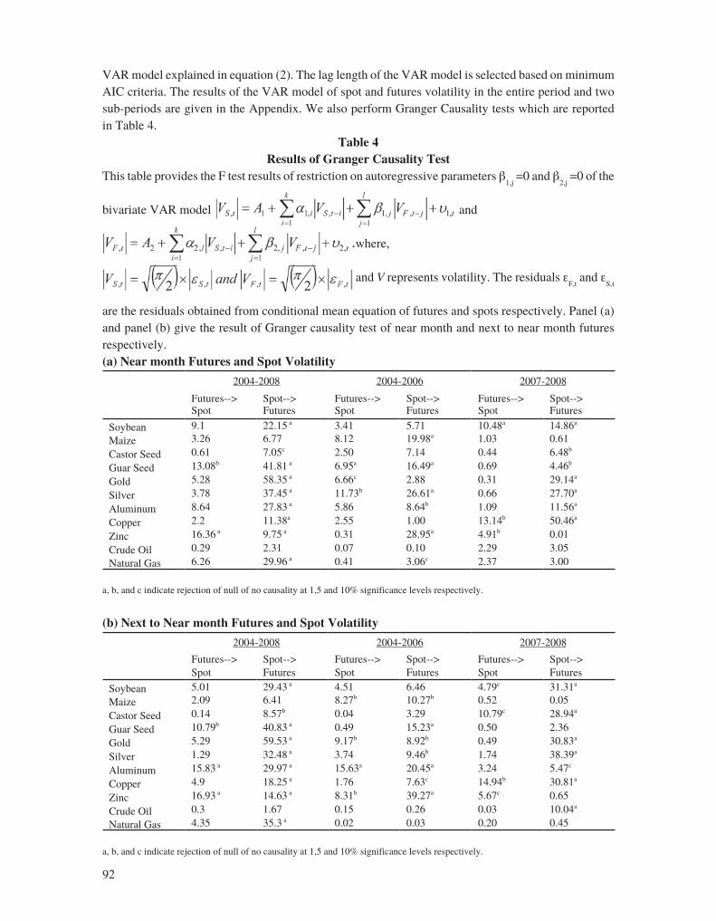
VAR model explained in equation (2). The lag length of the VAR model is selected based on minimum AIC criteria. The results of the VAR model of spot and futures volatility in the entire period and two sub-periods are given in the Appendix. We also perform Granger Causality tests which are reported in Table 4.

Table 4Results of Granger Causality Test

This table provides the F test results of restriction on autoregressive parameters β1,j

=0 and β2,j

=0 of the

bivariate VAR model and

where,

and V represents volatility. The residuals εF,t

and εS,t

are the residuals obtained from conditional mean equation of futures and spots respectively. Panel (a) and panel (b) give the result of Granger causality test of near month and next to near month futures respectively.(a) Near month Futures and Spot Volatility

2004-2008 2004-2006 2007-2008

Futures--> Spot

Spot--> Futures

Futures--> Spot

Spot--> Futures

Futures--> Spot

Spot--> Futures

Soybean 9.1 22.15 a 3.41 5.71 10.48a 14.86a

Maize 3.26 6.77 8.12 19.98a 1.03 0.61

Castor Seed 0.61 7.05c 2.50 7.14 0.44 6.48b

Guar Seed 13.08b 41.81 a 6.95a 16.49a 0.69 4.46b

Gold 5.28 58.35 a 6.66c 2.88 0.31 29.14a

Silver 3.78 37.45 a 11.73b 26.61a 0.66 27.70a

Aluminum 8.64 27.83 a 5.86 8.64b 1.09 11.56a

Copper 2.2 11.38a 2.55 1.00 13.14b 50.46a

Zinc 16.36 a 9.75 a 0.31 28.95a 4.91b 0.01

Crude Oil 0.29 2.31 0.07 0.10 2.29 3.05

Natural Gas 6.26 29.96 a 0.41 3.06c 2.37 3.00

a, b, and c indicate rejection of null of no causality at 1,5 and 10% significance levels respectively.

(b) Next to Near month Futures and Spot Volatility

2004-2008 2004-2006 2007-2008

Futures--> Spot

Spot--> Futures

Futures--> Spot

Spot--> Futures

Futures--> Spot

Spot--> Futures

Soybean 5.01 29.43 a 4.51 6.46 4.79c 31.31a

Maize 2.09 6.41 8.27b 10.27b 0.52 0.05

Castor Seed 0.14 8.57b 0.04 3.29 10.79c 28.94a

Guar Seed 10.79b 40.83 a 0.49 15.23a 0.50 2.36

Gold 5.29 59.53 a 9.17b 8.92b 0.49 30.83a

Silver 1.29 32.48 a 3.74 9.46b 1.74 38.39a

Aluminum 15.83 a 29.97 a 15.63a 20.45a 3.24 5.47c

Copper 4.9 18.25 a 1.76 7.63c 14.94b 30.81a

Zinc 16.93 a 14.63 a 8.31b 39.27a 5.67c 0.65

Crude Oil 0.3 1.67 0.15 0.26 0.03 10.04a

Natural Gas 4.35 35.3 a 0.02 0.03 0.20 0.45

a, b, and c indicate rejection of null of no causality at 1,5 and 10% significance levels respectively.

93

The results of volatility spillover between spot and futures markets for near-month and next-to-near-month futures indicate that there is bidirectional causality between spot and futures markets volatility for agricultural commodities. In the case of precious metals, the futures market leads the spot market in volatility spillover. However in the first sub-period, a bidirectional causality is observed. The clear dominance of futures markets is observed in the recent sub-period. In industrial metals where the LME spot prices are used by Indian exchanges, we again find bidirectional causality between spot and futures volatility. The bidirectional causality is more prominent in the next-to-near futures contracts of Aluminum and Zinc, and for both near and next-to-near futures of Copper. However, in the second sub-period, Aluminum futures lead the spot volatility; spot volatility leads the futures volatility in the case of Zinc and bidirectional causality exists in the case of Copper. It is interesting to note that for Zinc, though we do not find the effect of the LME price or return spillover, strong volatility spillover from the LME spot prices to Indian futures prices is found. As observed in the case of return spillover for energy commodities, Crude Oil and Natural Gas, the spot and futures market volatilities are independent and do not affect each other. The results of return and volatility spillover between the NYMEX spot prices and the Indian futures markets indicate that the NYMEX spot prices for energy commodities do not play a dominant role in the price discovery process in the Indian futures markets.

Further Discussion

Our investigations on price discovery through return and volatility spillovers indicate some important results: (a) we find differences in the relative importance of spot and futures markets in the price discovery process between agricultural and non-agricultural commodities, and (b) we also find that the relative importance of futures and spot markets in the price discovery process has changed in the recent sub-period. It is evident that for agricultural and non-agricultural commodities, the total volume and open interest have increased significantly in the recent period The speculation ratio, defined as the ratio of volume to open interest, has also increased, especially for non-agricultural commodities. In the case of industrial metals, the LME spot prices still play a significant role in the price discovery process in the Indian futures markets. However, this may be due to an increased and diverse participation (more speculation) in the futures market in the recent period, the dominant role of the LME spot prices has decreased in short-run price discovery. Our results support the conjecture that the increased volume in the futures markets may imply better price discovery and as the Indian futures markets are maturing, their role in price discovery is also likely to strengthen.

An alternative explanation could be based on the fact that the LME/NYMEX spot prices are polled prior to closing of the LME/ NYMEX futures. It is possible that the Indian futures prices assimilate information from the LME futures prices of industrial metals and similarly the NYMEX futures prices of energy commodities rather than their spot prices. Hence, we further analyze the lead-lag relationship in the LME/NYMEX futures, the Indian futures and the spot prices in a tri-variate model. First, these prices are tested for a cointegrated relationship and as shown in Table 5, we find that for industrial metals and Natural Gas, international futures prices, Indian futures prices and spot prices are cointegrated. In case of Crude Oil, we do not find cointegration across these prices. The results of the weak exogeneity test (Table 6) indicate that in case of Aluminum and Copper both LME and Indian futures prices are exogenous and spot prices adjust to maintain long-run equilibrium. In case of Zinc and Natural Gas, only Indian futures prices are exogenous. We also perform the Granger causality test (Table 7) and find that in the case of Aluminum, there is bidirectional causality between LME futures and Indian futures and Indian futures and spot prices.

94

Table 5Results of Johansen Cointegration Test of Indian Futures, International Futures and Spot

Prices for Industrial Metals and Energy Commodities

This table provides Maximum Eigenvalue and Rank of cointegration test of VECM (3) model where Indian futures, international futures and spot prices are used as endogenous variable.

CommodityLag length

Cointegration Rank Test Using Trace

Cointegration Rank Test Using Maximum Eigenvalue

with trend without trend with trend without trend

Aluminum

Rank=0 2 166.74* 166.80* 123.81* 123.81*

Rank=1 42.93* 42.99* 38.28* 38.28*

Rank=2 4.64 4.70 4.64 4.70

Copper

Rank=0 3 68.68* 71.99* 49.26* 49.26*

Rank=1 19.41* 22.72* 16.51* 17.27*

Rank=2 2.90 5.45 2.90 5.45

Zinc

Rank=0 93.39* 93.74* 52.01* 52.06*

Rank=1 41.37* 41.68* 36.75* 37.03*

Rank=2 4.62 4.64* 4.62 4.64

Crude Oil

Rank=0 3 48.46* 49.64* 37.34* 37.53*

Rank=1 11.12* 12.11* 9.39* 9.78*

Rank=2 1.72 2.32 1.72 2.32

Natural GasRank=0 2 129.35* 129.41* 74.40* 74.41*

Rank=1 54.94* 55.00* 50.41* 50.41*

Rank=2 4.53 4.58 4.53 4.5864

* denotes rejection of null at 5% significance level.

Table 6Results of Weak Exogeneity Test of Indian Futures, International Futures and Spot prices

This table provides results of weak exogeneity test which measures the speed of adjustment of prices towards the long run equilibrium relationship among Indian futures, international futures and spot prices

Int Futures India Futures Spot Prices

Commodity Chi-Square Chi-Square Chi-Square

Aluminum 4.34 26.69* 44.17*

Copper 3.31 3.86 35.95*

Zinc 31.84* 7.84 58.27*

Crude Oil -- -- --

Natural Gas 23.08* 2.78 44.79*

* denotes rejection of null at 5% significance level

95

Table 7Results of Granger Causality Test of Indian Futures, International Futures and Spot prices

This table provides the F test results of restriction on autoregressive parameters of VECM (3) models where Indian futures, LME futures and spot prices are taken as endogenous variables.

Int Futures --> India Futures

India Futures --> Int Futures

Int Futures --> Spot

Spot --> Int Futures

India Futures --> Spot

Spot --> India Futures

Aluminum 22.9** 28.00** 105.94** 1.44 94.55** 21.57**

Copper 5.20 129.15** 130.89** 5.64 368.74** 4.55

Zinc 5.04 74.52** 110.88** 1.14 229.81** 7.98*

Crude Oil -- -- -- -- -- --

Natural Gas 4.47 24.11** 15.44** 45.83** 157.79** 7.14*

** (*) denotes rejection of null at 1 and 5% significance level respectively.

Agricultural commodities have a seasonal production pattern while production of non-agricultural commodities depends on an economic cycle (Fama and French, 1987). Most of the commodities (Caster Seed and Guar Seed) are grown once in a year and the arrival of the commodity (or inventory buildup) happens in particular months. In our case, for all four commodities the arrival starts from the month of October and lasts for 5-6 months (the harvest period). After that inventories decline, supply of commodities is limited and hence the supply of arbitrage (availability of commodity for performing the arbitrage across markets) is also restricted in the lean period (the 5-6 months after arrival). We analyze the volume and open interest in these commodities and find that in all the commodities, the volume and open interest in the futures markets are high in the harvest period and low in the lean period (Figure 1). The lean period includes the crop sowing period where the decision regarding the area of cultivation is taken and this information may be more common among the participants in the spot markets compared to the futures markets participants because the nature of the participants is different in the two markets. These factors may result differences in the price discovery process during the harvest and the lean periods.

The lean period includes the crop sowing period where the decision regarding the area of cultivation is taken and this information may be more common among the participants in the spot markets compared to the futures markets participants as the nature of participants is different in the two markets. These factors may result in the differences in the price discovery process during the harvest and the lean periods.

An efficient futures market reflects the future demand and supply condition of an underlying and gives signals about the storage or selling of a storable commodity depending upon different future economic conditions. If it is assumed that in the initial phase of the Indian commodity futures markets, because of a lack of awareness, poor warehousing facilities and participation in the futures trading, the decision regarding the storage and selling of storable commodities is not reliable enough, this would lead to a skewed inventory holding pattern. In other words, it would be a high inventory and supply of commodity just after the harvest and less inventory and a limited supply in the lean period. However, in the recent period, the futures markets are providing relatively more awareness, higher

96

futures trading volume, and increased warehouse facilities, and therefore more reliable storage/selling signals. This may result in less of a skewed inventory and supply pattern, and hence in the recent period the futures markets are dominating the price discovery process.

Figure 1Monthly Average of Open Interest and Volume of Near Month Futures Contracts of

Agricultural Commodities

In order to understand the difference in spot-future price dynamics in agricultural commodities during both the lean and harvest periods, we divide the data of the agricultural commodities into these two periods. We apply the VECM model to understand the lead-lag relation in the harvest and lean periods. The results of weak exogeniety and the Granger Causality test in lean and harvest periods for the entire period and for two sub-periods are given in Table 8. The results indicate that in the harvest period where there is a high inventory and futures trading the volume including an open interest is high as compared to the lean period. The futures markets lead the price discovery process both in the long run as well as in the short run. The results of the weak exogeneity and the Granger causality

97

tests indicate that spot prices are influenced by futures prices and adjust to restore the long and the short-run equilibrium. However, in the lean period, we find that in most of the cases spot prices are weakly exogenous, i.e. futures prices adjust to restore long run equilibrium. The results of the Granger causality also indicate that there is bidirectional causality between spot and futures returns in the short run. The results of the entire period and both the sub-periods are similar.

Table 8Results of Weak Exogeniety and Granger Causality Test of Near Month Futures

This table provides results of weak exogeneity test which measures the speed of adjustment of prices towards the long run equilibrium relationship and Granger causality test which test the restriction on autoregressive parameters in harvest and lean period.

(a) The Entire Period (2004-2008)

Weak Exogeneity Test Granger Causality Test

Harvest Period Lean Period Harvest Period Lean PeriodFutures Prices

Spot Prices

Futures Prices

Spot Prices

Spot -> Futures

Futures -> Spot

Spot -> Futures

Futures -> Spot

Soy Bean 11.76a 42.92a 0.33 1.69 16.09a 68.09a 1.21 14.35a

Maize 1.25 11.33a 0.27 14.64a 1.07 11.55a 0.75 16.34a

Castor Seed 0.54 11.88a 4.33a 0.92 2.92 51.93a 9.96a 35.96a

Guar Seed 1.6 8.01a 13.88a 0.48 5.16 139.14a 20.02a 252.08a

a, b and c indicate the rejection of null at 1, 5 and 10% significance levels respectively.

(b) The First Sub-period (2004-2006)



Spot Prices

Futures Prices

Spot Prices

Spot -> Futures

Futures -> Spot

Spot -> Futures

Futures -> Spot

Soybean 1.51 23.81a 3.05c 4.03b 2.06 33.23a 1.69 53.59a

Maize 0.16 9.34a 0.04 13.55a 0.23 9.64a 8.63b 18.78a

Castor Seed 0.63 2.37 18.02a 0.4 3.54 34.42a 21.71a 60.1a

Guar Seed 0.13 17.11a 9.81a 0.24 3.33 135.24a 9.39b 208.26a


(c) The Second Sub-period (2007-2008)



Spot Prices

Futures Prices

Spot Prices

Spot -> Futures

Futures -> Spot

Spot -> Futures

Futures -> Spot

Soybean 0.96 9.22a 0 1.31 1.28 22.6a 1.18 9.29a

Maize 3.45c 4.83b 0.14 18.08a 2.14 4.9b 0.68 20.7a

Castor Seed 2.38 15.84a 0.92 0.56 2.43 16.78a 1.05 7.27a

Guar Seed 6.62b 0.43 2.85c 0.13 4.4 21.32a 4.93 48.91a


98

The difference in the role of spot and futures prices in the price discovery process during the harvest and the lean periods leads to bidirectional causality in spot-futures markets when the entire sample comprising the lean and harvest periods is analyzed together. It is important to note that in the second sub-period, the role of futures prices has strengthened in the harvest as well as in the lean period. As indicated earlier, because of increasing awareness of futures markets, high volume of futures trade, increasing warehouse facilities, and less policy restrictions on the movement of commodities, the role of the futures market in price discovery has improved in the more recent period.

Our findings have implications for market participants and policy makers in the Indian commodity futures market context. The Indian commodity futures markets are of recent origin and are still struggling with a relatively thin volume, low market depth, infrequent trading and non-awareness of futures markets among traders and farmers despite their having grown considerably since inception. Many times, the Indian commodity markets have been criticized for speculative activity, and futures trading on many agricultural commodities has been banned. Investigating and understanding the price discovery process of the Indian commodity futures markets therefore is important as it will help guide participants and policy makers to improve the efficiency of these commodity markets and to make the futures a successful instrument in the commodity market. Our results partially support the results of Yang et al. (2001), who found that most of the storable agricultural commodity futures are cointegrated with spot markets and perform a leading role in the price discovery process. In the case of industrial metals, our results are consistent with the results of Ferretti and Gounzalo (2007). An important finding of the study is that the price discovery process of agricultural commodities is different during the harvest from the lean period. It is found that in the harvest period, the futures markets lead the price discovery process unidirectionally whereas in the lean period both futures and spot markets affect each other and bidirectional causality exists between spot and futures prices. It is evident from our findings that the Indian commodity futures markets by and large lead the spot markets and this relationship has improved in the recent period because of a high volume and diverse participation in comparison to the low participation in the early stage of development.

CONCLUSIONS

In this paper, we investigate the effectiveness of the price discovery function of commodity futures markets of India through return and volatility spillovers between spot and futures markets of eleven commodities consisting of four agricultural commodities, two precious metals, three industrial metals and two energy commodities. Price discovery is a very important function of futures markets, and the theory suggests that an efficient futures market should be the main source of information dissemination as it responds more rapidly to future economic events (future demand and supply conditions) than does the spot market. The studies in the area of price discovery, which are mostly from developed markets and for non-agricultural commodities, tend to show that futures prices play a major role in the price discovery process. However, in emerging and thinly traded markets results have been mixed and, in some cases, the futures markets have failed to perform the effective role in the price discovery process. In the Indian context, where organized trading started in 2004, we try to understand empirically the role of the futures market in the price discovery process.

99

In the case of agricultural commodities, we find bidirectional spillover effects between spot and futures markets. In most of the cases, spot market and futures prices are cointegrated and both adjust to restore long run equilibrium relationship. In the short run also, return spillover is bidirectional. The volatility spillover results are also similar as return spillover and volatility spillover take place in both directions. On further analysis of the price discovery process in agricultural commodities during the harvest and the lean periods, we find that that in the harvest period, when the futures volume of trade is high, the futures markets lead the spot market both in the long as well as in the short run whereas in the lean period both markets jointly perform the function of price discovery. In the recent period, however, the role of futures markets in price discovery has strengthened.

For precious metals, Gold and Silver, there is a clear dominance of futures markets in both return and volatility spillovers in the recent period. The spot prices adjust to the long run equilibrium relationship and return and volatility spillovers take place from futures markets to spot markets. However, in case of Silver, the significant role of spot markets in the prices discovery process is observed. In the case of industrial metals, we find a very interesting result that the LME spot prices (which are taken as spot prices for settlement by Indian exchanges) play a significant role in the price discovery process in the Indian market. Both Indian futures prices and LME spot prices adjust to a long run equilibrium relationship. In both return and volatility, we find bidirectional spillover effects but in the recent period the effect of LME spot prices on futures prices in the short run price discovery has decreased. In the case of energy commodities, NYMEX spot prices have a limited effect on the long and short run price discovery for the spot market. However, we do not find evidence of a volatility spillover between spot and futures markets for these two commodities. We further analyze the lead-lag relationship between LME/NYMEX futures prices, Indian futures prices and spot prices of industrial metals and energy commodities and find that Indian futures prices are cointegrated with both international spot and futures prices except for Crude Oil. In the short run, bidirectional causality exists between Indian futures and LME/NYMEX spot prices.

To sum up, it can be concluded that in the Indian commodity futures markets, futures markets do not dominate the price discovery process as they do in other developed markets. In the case of agricultural commodities and industrial metals, the price discovery takes place in both spot and futures markets. For the precious metals and energy commodities, which are more tradable in nature, futures markets are not affected by spot markets. Nevertheless, in the recent two years, the price discovery role of futures markets has strengthened compared to the previous two years and may improve further in the future.

NOTES

1. Leading commodity futures contracts in terms of volume are Gold, Crude, Natural Gas, and Silver futures traded at NYMEX in US, Aluminum, Copper, and Zinc futures traded at LME, London, and Corn, Soybean contracts at CBOT in the US. Details are available [on line] at: http://www.futuresindustry.org/files/pdf/Jul-Aug_FIM/Jul-Aug_Volume.pdf

2. Basic characteristics of spot and futures returns can be obtained from the authors.

100

REFERENCES

Abhyankar, A. (1998). “Linear and Nonlinear Granger Causality: Evidence from the U.K. Stock Index Futures Market,” Journal of Futures Markets, 18: 519-540.

Antoniou, A. and Ergul, N. (1997). “Market Efficiency, Thin Trading and Non-linear Behavior: Evidence from an Emerging Market,” European Financial Management, 3: 175-90.

Antoniou, A., and Garrett, I. (1993). “To What Extent did Stock Index Futures Contribute to the October 1987 Stock Market Crash?,” Economic Journal, 103: 1444-1461.

Antoniou, A., Pescetto, G., and Violaris, A. (2001). “Modeling International Price Relationships and Interdependencies between EU Stock Index and Stock Index Futures Markets: A Multivariate Analysis,” Working Paper, Centre for Empirical Research in Finance, Department of Economics and Finance, University of Durham.

Azizan, N.A., Ahmad N., and Shannon, S. (2007). “Is the Volatility Information Transmission Process between the Crude Palm Oil Futures Market and Its Underlying Instrument Asymmetric?,” International Review of Business Research Papers, 3: 54-77.

Bakaert, G. and Harvey, C.R. (1997). “Emerging Equity Market Volatility,” Journal of Financial Economics, 43: 29-77.

Brockman, P. and Tse, Y. (1995). “Information Shares in Canadian Agricultural Cash and Futures Markets,” Applied Economics Letters, 2: 335-338.

Brooks, C., Rew, A.G., and Ritson, S. (2001). “A Trading Strategy based on the Lead-Lag Relationship between the Spot Index and Futures Contract for the FTSE 100,” International Journal of Forecasting, 17: 31-44.

Carter, C.A. (1989). “Arbitrage Opportunities between Thin and Liquid Futures Markets,” Journal of Futures Markets, 9: 347-353.

Chan, K. (1992). “A Further Analysis of the Lead–Lag Relationship between the Cash Market and Stock Index Futures Market,” Review of Financial Studies, 5: 123-152

Chan, K., Chan, K.C., and Karolyi, G.A. (1991). “Intraday Volatility in the Stock Index and Stock Index Futures Markets,” Review of Financial Studies, 4: 657-684.

Chang, E., Jain, P., and Locke, P. (1995). “Standard & Poor’s 500 Index Futures Volatility and Price Changes around the New York Stock Exchange Close,” Journal of Business, 68: 61-84.

Cheung, Y.W., and Ng, L.K. (1990). “The Dynamics of S&P 500 Index and S&P 500 Futures Intraday Price Volatilities,” Review of Futures Markets, 9: 458-486.

101

Evans, E.B. (1978). “Country Elevator Use of the Market,” in A. Peck (ed.), Views from the Trade. Chicago: Board of Trade of the City of Chicago.

Floros, C. and Vougas, D.V. (2007). “Lead-Lag Relationship between Futures and Spot Markets in Greece: 1999 – 2001,” International Research Journal of Finance and Economics, 7: 168-174.

Fortenberry, T.R. and Zapata, H.O. (1997). “An Evaluation of Price Linkages between Futures and Cash Markets for Cheddar Cheese,” Journal of Futures Markets, 17: 279-301.

Gardbade, K.D., and Silber, W.L. (1983). “Price Movements and Price Discovery in Futures and Cash Markets,” Review of Economics and Statistics, 65: 289-297.

Hasbrouck, J. (1995). “One Security, Many Markets: Determining the Contributions to Price Discovery,” Journal of Finance, 50: 1175-1199.

Herbst, A., McCormack, J., and West, E. (1987). “Investigation of a Lead-Lag Relationship between Spot Indices and Their Futures Contracts,” Journal of Futures Markets, 7: 373-381.

Hodgson, A., Masih, A.M.M., and Masih, R. (2006). “Futures Trading Volume as a Determinant of Prices in Different Momentum Phases,” International Review of Financial Analysis, 15: 68-85.

Kavussanos M.G., Visvikis, I.G., and Alexakis, P.D. (2008). “The Lead-Lag Relationship between Cash and Stock Index Futures in a New Market,” European Financial Management, 14: 1007-1025

Kawaller, I.G., Koch, P.D., and Koch, T.W. (1987). “The Temporal Price Relationship between S&P 500 Futures and the S&P 500 Index,” Journal of Finance, 42: 1309-1329.

Kolamkar, D. S. (2003). “Regulation and Policy Issues for Commodity Derivatives in India.” Accessed on 20, January, 2009 and available [online] at:http://www.igidr.ac.in/~susant/DERBOOK/PAPERS/dsk_draft1.pdf

Mattos, F., and Garcia, P. (2004). “Price Discovery in Thinly Traded Markets: Cash and Futures Relationships in Brazilian Agricultural Futures Markets,” Paper presented at the NCR-134 Conference on Applied Commodity Price Analysis, Forecasting, and Market Risk Management

Maynard, L.J., Hancock, S., and Hoagland, H. (2001). “Performance of Shrimp Futures Markets as Price Discovery and Hedging Mechanisms,” Agriculture Economics and Management, 5: 115-128.

Min, J.H. and Najand, M. (1999). “A Further Investigation of the Lead-Lag Relationship between the Spot and Stock Index Futures: Early Evidence from Korea,” Journal of Futures Markets, 19: 217-232.

Naik, G. and Jain, S.K. (2002). “Indian Agricultural Commodity Futures Markets: A Performance Survey,” Economic and Political Weekly, XXXVII (30).

Nair, C.K.G. (2004). “Commodity Futures Markets in India: Ready for “Take-Off?,” NSE News, July.

102

Oellermann, C.M., Brorsen, B.W., and Farris, P.L. (1989). “Price Discovery for Feeder Cattle,” Journal of Futures Markets, 9: 113-121.

Roy, A. and Kumar, B. (2007). “A Comprehensive Assessment of Wheat Futures Market: Myths and Reality,” Paper presented at International Conference on Agribusiness and Food Industry in Developing Countries: Opportunities and Challenges, held at IIM Lucknow (August).

Sahadevan, K.G. (2002). “Sagging Agricultural Commodity Exchanges: Growth Constraints and Revival Policy Options,” Economic and Political Weekly, XXXVII (30).

Silber, W. (1981). “Innovation, Competition, and New Contract Design in Futures Markets,” Journal of Futures Markets, 1: 123-155.

Schroeder, T.C., and Goodwin, B.K. (1991). “Price Discovery and Cointegration for Live Hogs,” Journal of Futures Markets, 11: 685-696.

Stoll, H.R., and Whaley, R.E. (1990). “The Dynamics of Stock Index and Stock Index Futures Returns,” Journal of Financial and Quantitative Analysis, 25: 441-468.

Schwert, G.W. (1989). “Why does Stock Market Volatility Change over Time?” Journal of Finance, 44: 1115-1153.

Schwert, G.W. (1990). “Stock Volatility and the Crash of ’87,” Review of Financial Studies, 3: 77-102.

Thomas, S. (2003). “Agricultural Commodity Markets in India: Policy Issues for Growth,” Mimeo, Indira Gandhi Institute for Development Research, Mumbai, India.

Thomas, S., and Karande, K. (2002). “Price Discovery across Multiple Spot and Futures Markets.” Available [online] at:http://www.igidr.ac.in/~susant/PDFDOCS/ThomasKarande2001_pricediscovery_castor.pdf.

Tomek, W.G. (1980). “Price Behavior on a Declining Terminal Market,” American Journal of Agricultural Economics, 62: 434-445.

Tse, Y. (1999). “Price Discovery and Volatility Spillovers in the DJIA Index and Futures Market,” Journal of Futures Markets, 19: 911–930.

Working, H. (1962). “New Concepts Concerning Futures Markets and Prices,” American Economic Review, 52: 431-459.

Yang, J., Bessler, D.A., and Leatham, D.J. (2001). “Asset Storability and Price Discovery in Commodity Futures Markets: A New Look,” Journal of Futures Markets, 21: 279-300.

103

APPENDIX

Table 1(a)Results of ADF Unit Root Test: Near-Month Futures

2004-2008 2004-2006 2007-2008

Commodity Price Return Price Return Price Return

Soybean 1.99 -9.36a 23.1a -6.94a 1.4 -5.49a

Maize 1.88 -8.03a 4.76 -5.41a 2.21 -6.43a

Castor Seed 1.26 -7.8a 6.46 -5.9a 2.18 -4.76a

Guar Seed 6.1 -10.04a 7.71b -8.01a 3.53 -5.39a

Gold 2.43 -7.98a 1.94 -4.99a 2.68 -5.9a

Silver 1.52 -8.96a 2.25 -5.82a 1.78 -6.67a

Aluminum 3.42 -7.04a 3.2 -4.13a 1.53 -4.88a

Copper 1.26 -7.14a 1.51 -4.22a 3.2 -5.6a

Zinc 2.32 -8.19a 2.16 -5.67a 4.02 -6.09a

Crude Oil 2.74 -8.62a 3.04 -5.34a 1.82 -6.44a

Natural Gas 2.21 -5.65a 1.73 -2.56b 2.23 -4.72a

a, and b indicate rejection of null at 1 and 5% significant levels respectively

Table 1(b) Results of ADF Unit Root Test: Next-to–Near-Month Futures

2004-2008 2004-2006 2007-2008


Soybean 1.77 -9.51a 6.37b -6.7a 1.76 -6.02a

Maize 1.54 -8.24a 2.53 -5.18a 2.46 -6.3a

Castor Seed 1.41 -7.4a 4.78 -5.8a 1.89 -4.15a

Guar Seed 6.52b -9.99a 7.28b -7.95a 3.61 -5.5a

Gold 2.38 -8.01a 1.89 -5.08a 2.73 -5.88a

Silver 1.54 -8.8a 2.45 -5.61a 1.95 -6.64a

Aluminum 3.45 -7.4a 2.94 -4.57a 1.54 -4.95a

Copper 1.19 -7.12a 1.69 -4.2a 2.88 -5.65a

Zinc 2.26 -7.9a 2.07 -5.89a 3.83 -5.98a

Crude Oil 2.67 -8.55a 2.89 -5.27a 1.68 -6.38a

Natural Gas 2.09 -5.31a 2.27 -2.37b 2.52 -4.5a


104

Table 1(c)Results of ADF Unit Root Test: Spot

2004-2008 2004-2006 2006-2008


Soybean 1.97 -7.46a 28.39a -6.63a 1.26 -3.75a

Maize 3.19 -7.73a 5.18 -5.37a 1.50 -5.34a

Castor Seed 1.59 -7.42a 3.96 -5.57a 2.22 -4.85a

Guar Seed 5.34 -9.63a 6.99b -7.52a 2.71 -5.73a

Gold 2.35 -8.10a 2.01 -5.34a 2.66 -5.89a

Silver 1.33 -9.09a 2.25 -6.26a 1.60 -6.25a

Aluminum 3.70 -6.53a 3.99 -3.92a 1.79 -5.11a

Copper 1.25 -7.61a 1.48 -5.36a 2.73 -5.28a

Zinc 2.51 -6.68a 2.48 -3.56a 4.51 -5.75a

Crude Oil 2.67 -9.13a 3.4 -5.97a 1.39 -6.85a

Natural Gas 2.31 -7.37a 2.21 -3.63a 2.23 -5.69a


Table 2(a) Johansen Cointegration Test Results: Near-Month Futures for the Entire Period

(2004-2008)

CommodityLag length




Soybean H0:Rank=0 5 75.141b 75.142b 72.966b 72.967b

H1:Rank=1 2.175 2.175 2.175 2.175

Corn H0:Rank=0 1 34.338b 34.341b 30.388b 30.389b

H1:Rank=1 3.950b 3.952 3.950b 3.952

Castor Seed H0:Rank=0 2 37.264b 37.264b 36.133b 36.133b

H1:Rank=1 1.130 1.130 1.130 1.130

Guar Seed H0:Rank=0 4 52.006b 52.006b 43.152b 43.152b

H1:Rank=1 8.854b 8.854 8.854b 8.854

Gold H0:Rank=0 5 63.918b 63.948b 59.795b 59.822b

H1:Rank=1 4.124b 4.126 4.124b 4.126

Silver H0:Rank=0 4 77.626b 77.628b 74.371b 74.373b

H1:Rank=1 3.254 3.254 3.254 3.254

Aluminum H0:Rank=0 4 39.008b 39.012b 34.759b 34.760b

H1:Rank=1 4.249b 4.253 4.249b 4.253

Copper H0:Rank=0 5 48.682b 48.723b 46.710b 46.721b

H1:Rank=1 1.972 2.002 1.972 2.002

Zinc H0:Rank=0 2 208.095b 208.095b 206.284b 206.284b

H1:Rank=1 1.811 1.811 1.811 1.811

Crude Oil H0:Rank=0 3 128.490b 128.498b 124.773b 124.778b

H1:Rank=1 3.718 3.720 3.718 3.720

Natural Gas H0:Rank=0 2 129.593b 129.595b 125.823b 125.823b

H1:Rank=1 3.771 3.772 3.771b 3.772

105

Table 2(b)Johansen Cointegration Test Results:

Near-Month Futures for the First Sub-period (2004-2006)

CommodityLag length




Soybean H0:Rank=0 -- -- -- -- --

H1:Rank=1 -- -- -- --

Corn H0:Rank=0 4 16.688b 17.4399 14.7076b 15.1139

H1:Rank=1 1.9804 2.326 1.9804 2.326


H1:Rank=1 7.4819b 7.743 7.4819b 7.743

Guar Seed H0:Rank=0 -- -- -- -- --

H1:Rank=1 -- -- -- --

Gold H0:Rank=0 4 33.2712b 35.3758b 31.886b 31.8861b

H1:Rank=1 1.3852 3.4897 1.3852 3.4897


H1:Rank=1 1.4146 3.3828 1.4146 3.3828

Aluminum H0:Rank=0 4 17.1062b 17.6303 11.4322 11.6102

H1:Rank=1 5.674b 6.0201 5.674 6.0201


H1:Rank=1 3.4089 6.3981 3.4089 6.3981

Zinc H0:Rank=0 4 26.4097b 27.5055b 21.2213b 21.5693b

H1:Rank=1 5.1885b 5.9362 5.1885b 5.9362


H1:Rank=1 4.1351b 4.5159 4.1351b 4.5159


H1:Rank=1 3.1098 3.1137 3.1098 3.1137

106

Table 2(c)Johansen Cointegration Test Results:

Near-Month Futures for the Second Sub-period (2007-2008)

CommodityLag length





H1:Rank=1 2.0309 2.2813 2.0309 2.2813

Corn H0:Rank=0 2 53.6334b 54.3634b 51.9219b 52.243b

H1:Rank=1 1.7115 2.1203 1.7115 2.1203


H1:Rank=1 0.5973 5.4208 0.5973 5.4208

Guar Seed H0:Rank=0 3 14.443 14.7208 10.3946 10.5972

H1:Rank=1 4.0483b 4.1236 4.0483b 4.1236

Gold H0:Rank=0 5 34.2115b 36.6046b 33.8792b 33.9065b

H1:Rank=1 0.3323 2.6982 0.3323 2.6982


H1:Rank=1 2.8705 2.9338 2.8705 2.9338


H1:Rank=1 1.8831 1.8999 1.8831 1.8999


H1:Rank=1 0.0047 0.5029 0.0047 0.5029

Zinc H0:Rank=0 3 92.5959b 95.264b 90.2879b 90.3328b

H1:Rank=1 2.308 4.9312 2.308 4.9312


H1:Rank=1 0.6692 3.1262 0.6692 3.1262


H1:Rank=1 2.1755 2.3519 2.1755 2.3519

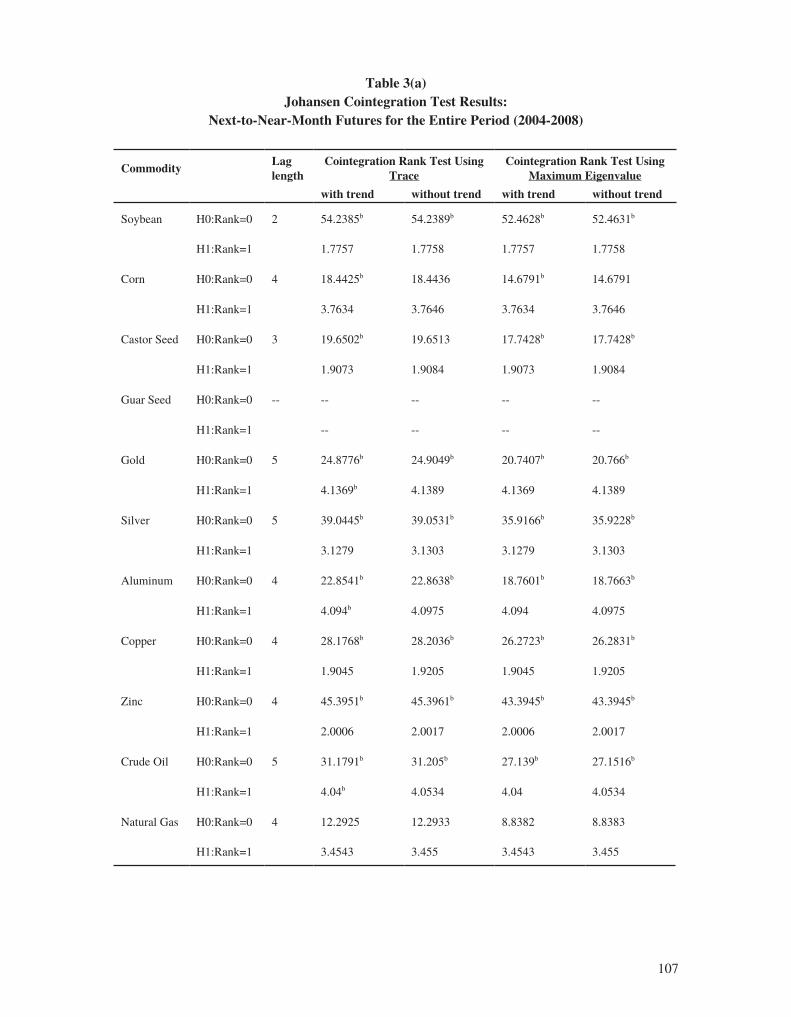
107

Table 3(a)Johansen Cointegration Test Results:

Next-to-Near-Month Futures for the Entire Period (2004-2008)

CommodityLag length





H1:Rank=1 1.7757 1.7758 1.7757 1.7758

Corn H0:Rank=0 4 18.4425b 18.4436 14.6791b 14.6791

H1:Rank=1 3.7634 3.7646 3.7634 3.7646

Castor Seed H0:Rank=0 3 19.6502b 19.6513 17.7428b 17.7428b

H1:Rank=1 1.9073 1.9084 1.9073 1.9084

Guar Seed H0:Rank=0 -- -- -- -- --

H1:Rank=1 -- -- -- --

Gold H0:Rank=0 5 24.8776b 24.9049b 20.7407b 20.766b

H1:Rank=1 4.1369b 4.1389 4.1369 4.1389


H1:Rank=1 3.1279 3.1303 3.1279 3.1303


H1:Rank=1 4.094b 4.0975 4.094 4.0975


H1:Rank=1 1.9045 1.9205 1.9045 1.9205

Zinc H0:Rank=0 4 45.3951b 45.3961b 43.3945b 43.3945b

H1:Rank=1 2.0006 2.0017 2.0006 2.0017


H1:Rank=1 4.04b 4.0534 4.04 4.0534

Natural Gas H0:Rank=0 4 12.2925 12.2933 8.8382 8.8383

H1:Rank=1 3.4543 3.455 3.4543 3.455

108

Table 3(b)Johansen Cointegration Test Results: Next-to-Near-Month Futures for the First Sub-period

(2004-2006)

CommodityLag length




Soybean H0:Rank=0 -- -- -- -- --

H1:Rank=1 -- -- -- --

Corn H0:Rank=0 5 9.774 11.0376 9.6661 9.9421

H1:Rank=1 0.1079 1.0955 0.1079 1.0955

Castor Seed H0:Rank=0 5 16.7932b 16.905 10.4942 10.5601

H1:Rank=1 6.299 6.3449 6.299 6.3449

Guar Seed H0:Rank=0 -- -- -- -- --

H1:Rank=1 -- -- -- --

Gold H0:Rank=0 4 17.3307b 19.6357 15.9018b 16.059b

H1:Rank=1 1.4289 3.5767 1.4289 3.5767


H1:Rank=1 1.5506 3.2194 1.5506 3.2194

Aluminum H0:Rank=0 4 13.9602 14.6018 8.765 8.9065

H1:Rank=1 5.1953 5.6952 5.1953 5.6952

Copper H0:Rank=0 4 11.2417 15.0264 8.4567 9.017

H1:Rank=1 2.785 6.0094 2.785 6.0094

Zinc H0:Rank=0 4 16.2186b 17.3279 10.9552 11.2131

H1:Rank=1 5.2634 6.1148 5.2634 6.1148


H1:Rank=1 3.8884b 4.4252 3.8884 4.4252


H1:Rank=1 3.0529 3.0546 3.0529 3.0546

109

Table 3(c) Johansen Cointegration Test Results: Next-to-Near-Month Futures for the Second Sub-period

(2007-2008)

CommodityLag length





H1:Rank=1 2.2288 2.3203 2.2288 2.3203

Corn H0:Rank=0 2 44.7551b 45.5141b 40.3537b 40.9765b

H1:Rank=1 4.4014b 4.5376 4.4014b 4.5376

Castor Seed H0:Rank=0 2 5.9474 11.1229 4.9177 7.7606

H1:Rank=1 1.0298 3.3623 1.0298 3.3623

Guar Seed H0:Rank=0 3 17.7239b 17.9007 13.4506 13.4931

H1:Rank=1 4.2734b 4.4076 4.2734 4.4076

Gold H0:Rank=0 5 15.3198 17.6768 14.9115b 15.1356

H1:Rank=1 0.4083 2.5413 0.4083 2.5413


H1:Rank=1 2.528 2.6123 2.528 2.6123


H1:Rank=1 2.2417 2.287 2.2417 2.287


H1:Rank=1 0.0215 0.5348 0.0215 0.5348

Zinc H0:Rank=0 4 50.1037b 53.2048b 48.1382b 48.172b

H1:Rank=1 1.9656 5.0328 1.9656 5.0328

Crude Oil H0:Rank=0 5 13.4509 15.9838 12.235 12.4374

H1:Rank=1 1.2158 3.5464 1.2158 3.5464


H1:Rank=1 2.3597 2.616 2.3597 2.616

110

Table 4(a) Estimates of VECM Model: Near-Month Futures for the Entire Period (2004-2008)

Spot Prices:

CS

cS,EC

γF,EC

cS,1

cS,2

cS,3

cS,4

γF,1

γF,2

γF,3

γF,4

Soybean -0.064a -0.299a 0.307a -0.085 0.010 -0.063 -0.029 0.152a -0.040 -0.025 0.028

Maize 0.005a -0.042a 0.041a 0.148a 0.038 0.136a -- 0.058b 0.043 0.009 --

Castor Seed -0.002a -0.074a 0.074a -0.350a -0.043 -- -- 0.454a 0.067 -- --

Guar Seed -0.015 -0.032 0.034 -0.520a -0.203a -0.008 0.668a 0.214a 0.044 --

Gold 0.011a -0.191a 0.190a -0.577a -0.259a -0.112b -0.083 a 0.806a 0.472a 0.235a 0.105b

Silver 0.026a -0.177a 0.175a -0.481a -0.239a -0.105a -0.097 a 0.685a 0.331a 0.195a 0.098a

Aluminum -0.008a -0.142a 0.143a -0.329a -0.145a -0.091a 0.545a 0.223a 0.068 --

Copper 0.016a -0.177a 0.174a -0.618a -0.362a -0.159a 0.011 0.78a 0.545a 0.283a 0.126a

Zinc -0.013a -0.464a 0.466a -0.297a -0.137a -0.060b -- 0.418a 0.282a 0.126a --

Crude Oil -0.032a -0.354a 0.358a -0.228a -0.052 -- -- 0.589a 0.221a -- --

Natural Gas -0.038a -0.515a 0.522a -0.140a -- -- -- 0.240a -- -- --

a, b, and c denote significance of estimates at 1%, 5%, and 10% significant levels respectively.

Futures Prices:

CF

cF,EC

γS,EC

cF,1

cF,2

cF,3

cF,4

γS,1

γS,2

γS,3

γS,4

Soybean -0.027a -0.125a 0.129a -0.164a -0.180a -0.127b -0.032 0.168 a 0.153 b 0.077 0.089

Maize 0.001 -0.008 0.008 -0.007 -0.039 0.050 -- 0.089 0.078 0.025 --

Castor Seed 0.002b 0.047c -0.048c 0.166a 0.098 -- -- -0.148b 0.019 -- --

Guar Seed 0.052a 0.108a -0.115a 0.132a -0.033 -0.033 -- -0.034 -0.013 0.131a --

Gold -0.003 0.075 -0.075 0.085 0.002 0.047 0.015 -0.012 0.004 0.072 -0.047

Silver -0.021b 0.148a -0.146a 0.060 0.016 0.149a -0.011 -0.060 0.016 0.023 -0.068c

Aluminum 0.006b 0.098b -0.099b 0.058 -0.118b -0.061 -- 0.114 0.098 0.096 --

Copper -0.007 0.079 -0.078 0.054 0.173b 0.116 0.195a -0.196a -0.111 -0.118 -0.023

Zinc -0.002 -0.050 0.050 -0.044 -0.046 -0.054 0.049 0.041 0.033 --

Crude Oil 0.001 0.001 -0.001 -0.071 -0.060 -- 0.077 -0.015 -- --

Natural Gas 0.004 0.051 -0.051 0.053 -- -- -0.036 -- -- --


111

Table 4(b) Estimates of VECM Model: Near Month Futures for the First Sub-period (2004-2006)

Spot Prices:

CS

cS,EC

γF,EC

cS,1

cS,2

cS,3

cS,4

γF,1

γF,2

γF,3

γF,4

Soybean 0.000 -- -- 0.041 -0.124b -0.212 0.060 0.492 0.125b 0.162 0.134b

Maize 0.028a -0.050a 0.046a 0.140a 0.015 0.186a -- 0.075 0.064 -0.019 --

Castor Seed -0.028a -0.052a 0.057a -0.321a -- -- -- 0.482a -- -- --

Guar Seed 0.001b -- -- -0.534 -0.251 -0.032 -- 0.822 0.271 0.131 --

Gold 0.067a -0.290a 0.282a -0.441a -0.165a 0.005 -- 0.686a 0.386a 0.145b --

Silver 0.033a -0.184a 0.180a -0.431a -0.247a -0.174a -0.105a 0.696a 0.334a 0.243a 0.167a

Aluminum -0.045 -0.075b 0.084b -0.250a -0.129 -0.099 -- 0.482a 0.151b 0.044 --

Copper 0.057a -0.242a 0.232a -0.631a -0.342a -0.115a -- 0.796a 0.667a 0.280a --

Zinc -0.088a -0.345a 0.362a -0.259a -0.115 -0.161a -- 0.492a 0.178 0.153 --

Crude Oil -0.006a -0.325a 0.325a -0.180a -0.103a -- -- 0.542a 0.210a -- --

Natural Gas -0.427a -0.404a 0.477a -- -- -- -- -- -- -- --


Futures Prices:

CF

cF,EC

γS,EC

cF,1

cF,2

cF,3

cF,4

γS,1

γS,2

γS,3

γS,4

Soybean 0.000 -- -- 0.022 0.012 0.042 0.058 0.017 -0.038 -0.071 0.005

Maize 0.013 -0.021 0.020 -0.009 -0.053 0.022 -- 0.137b 0.123 0.072 --

Castor Seed 0.026b 0.049b -0.053b 0.174a -- -- -- -0.069 -- -- --

Guar Seed 0.000 -- -- -0.018 -0.030 0.114b -- 0.086 -0.027 0.006 --

Gold -0.001 0.007 -0.007 -0.087 -0.135 -0.067 -- 0.160 0.171 0.163a --

Silver -0.05a 0.293a -0.288a 0.082 0.048 0.241b 0.042 -0.151 -0.022 -0.034 -0.075

Aluminum 0.075b 0.122b -0.137b 0.046 -0.103 -0.142 -- 0.159 0.209b 0.265a --

Copper 0.020 -0.079 0.076 -0.144 -0.052 -0.032 -- 0.052 0.080 0.090b --

Zinc 0.024 0.085 -0.089 0.083 -0.068 0.024 -- 0.019 0.033 0.141 --

Crude Oil 0.000 -0.019 0.019 -0.159b -0.130 -- -- 0.130 -0.006 -- --

Natural Gas 0.1214 0.1154 -0.136 -- -- -- -- -- -- -- --


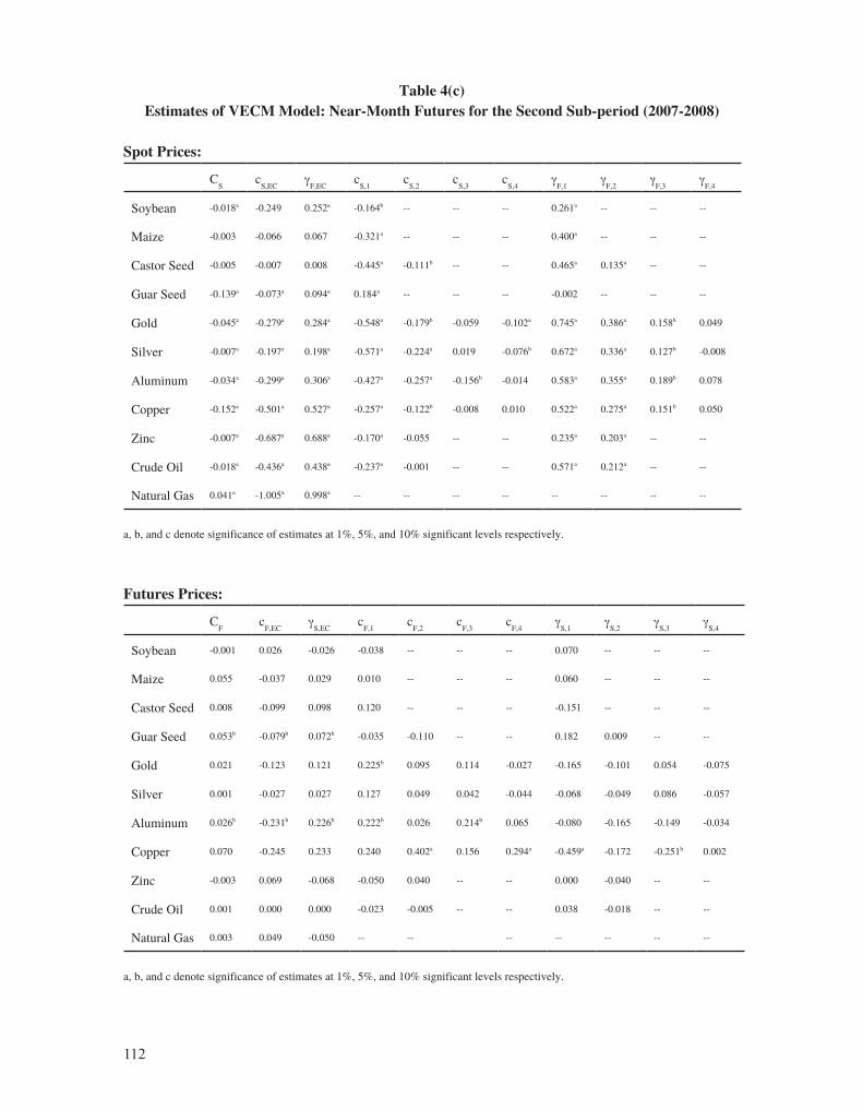
112

Table 4(c) Estimates of VECM Model: Near-Month Futures for the Second Sub-period (2007-2008)

Spot Prices:

CS

cS,EC

γF,EC

cS,1

cS,2

cS,3

cS,4

γF,1

γF,2

γF,3

γF,4

Soybean -0.018a -0.249 0.252a -0.164b -- -- -- 0.261a -- -- --

Maize -0.003 -0.066 0.067 -0.321a -- -- -- 0.400a -- -- --

Castor Seed -0.005 -0.007 0.008 -0.445a -0.111b -- -- 0.465a 0.135a -- --

Guar Seed -0.139a -0.073a 0.094a 0.184a -- -- -- -0.002 -- -- --

Gold -0.045a -0.279a 0.284a -0.548a -0.179b -0.059 -0.102a 0.745a 0.386a 0.158b 0.049

Silver -0.007a -0.197a 0.198a -0.571a -0.224a 0.019 -0.076b 0.672a 0.336a 0.127b -0.008

Aluminum -0.034a -0.299a 0.306a -0.427a -0.257a -0.156b -0.014 0.583a 0.355a 0.189b 0.078

Copper -0.152a -0.501a 0.527a -0.257a -0.122b -0.008 0.010 0.522a 0.275a 0.151b 0.050

Zinc -0.007a -0.687a 0.688a -0.170a -0.055 -- -- 0.235a 0.203a -- --

Crude Oil -0.018a -0.436a 0.438a -0.237a -0.001 -- -- 0.571a 0.212a -- --

Natural Gas 0.041a -1.005a 0.998a -- -- -- -- -- -- -- --


Futures Prices:

CF

cF,EC

γS,EC

cF,1

cF,2

cF,3

cF,4

γS,1

γS,2

γS,3

γS,4

Soybean -0.001 0.026 -0.026 -0.038 -- -- -- 0.070 -- -- --

Maize 0.055 -0.037 0.029 0.010 -- -- -- 0.060 -- -- --

Castor Seed 0.008 -0.099 0.098 0.120 -- -- -- -0.151 -- -- --

Guar Seed 0.053b -0.079b 0.072b -0.035 -0.110 -- -- 0.182 0.009 -- --

Gold 0.021 -0.123 0.121 0.225b 0.095 0.114 -0.027 -0.165 -0.101 0.054 -0.075

Silver 0.001 -0.027 0.027 0.127 0.049 0.042 -0.044 -0.068 -0.049 0.086 -0.057

Aluminum 0.026b -0.231b 0.226b 0.222b 0.026 0.214b 0.065 -0.080 -0.165 -0.149 -0.034

Copper 0.070 -0.245 0.233 0.240 0.402a 0.156 0.294a -0.459a -0.172 -0.251b 0.002

Zinc -0.003 0.069 -0.068 -0.050 0.040 -- -- 0.000 -0.040 -- --

Crude Oil 0.001 0.000 0.000 -0.023 -0.005 -- -- 0.038 -0.018 -- --

Natural Gas 0.003 0.049 -0.050 -- -- -- -- -- -- --


113

Table 5(a) Estimates of VECM Model: Next-to-Near-Month Futures for the Entire Period (2004-2008)

Spot Prices:

CS

cS,EC

γF,EC

cS,1

cS,2

cS,3

cS,4

γF,1

γF,2

γF,3

γF,4

Soybean -0.064a -0.088a 0.097a -0.083b -- -- -- 0.286a -- -- --

Maize 0.007a -0.022a 0.021a 0.173a 0.055 0.135a 0.050c 0.029 0.029 --

Castor Seed -0.019a -0.039a 0.043 -0.403a -0.058 -- -- 0.508a 0.101b -- --

Guar Seed 0.001a -- ---0.514

a-0.238a -0.034 -- 0.720a 0.255 a 0.116 a --

Gold 0.001b -0.053b 0.053b -0.686a -0.341a -0.161a -0.097a 0.947a 0.563a 0.301a 0.138a

Silver 0.020a -0.090a 0.088a -0.550a -0.279a -0.114a -0.096a 0.797a 0.397a 0.228a 0.101a

Aluminum -0.019a -0.063a 0.067a -0.368a -0.135a -0.070b -- 0.601a 0.229a 0.038 --

Copper 0.006a -0.056a 0.055a -0.645a -0.389a -0.177a -0.006 1.016a 0.677a 0.393a 0.168a

Zinc -0.025a -0.241a 0.246a -0.430a -0.202a -0.080a -- 0.648a 0.410a 0.172a --

Crude Oil -0.025a -0.102a 0.105a -0.446a -0.284a -0.163a -0.076a 0.897a 0.477a 0.280a 0.126a

Natural Gas 0.003b -- -- -0.432a -0.219a -0.081b -- 0.990a 0.442a 0.329a --


Futures Prices:

CF

cF,EC

γS,EC

cF,1

cF,2

cF,3

cF,4

γS,1

γS,2

γS,3

γS,4

Soybean -0.021a -0.029a 0.031a -0.014 -- -- -- 0.000 -- -- --

Maize 0.004 -0.011 0.010 -0.036 -0.054 0.071c -- 0.098c 0.025 -0.056 --

Castor Seed -0.004 -0.008 0.009 0.115b 0.064 -- -- -0.134b 0.039 -- --

Guar Seed 0.000b -- -- 0.036 -0.043 -0.018 -- 0.020 0.003 0.134a --

Gold 0.000 0.056c -0.056c 0.076 -0.021 0.051 0.034 0.007 0.005 0.054 -0.057

Silver -0.021b 0.103b -0.101b 0.027 -0.006 0.159b -0.013 -0.032 0.011 0.014 -0.068c

Aluminum 0.015b 0.050b -0.052b 0.080 -0.039 -0.060 -- 0.051 0.052 0.083b --

Copper -0.005c 0.044c -0.043c 0.027 0.104 0.077 0.173a -0.124 -0.071 -0.085 -0.021

Zinc -0.006 -0.047 0.048 -0.022 -0.005 -0.033 -- 0.022 0.017 0.028 --

Crude Oil 0.009 0.035 -0.036 -0.029 -0.011 0.080 0.036 0.038 -0.063 -0.048 0.031

Natural Gas -0.001 -- -- 0.000 -0.011 -0.050 -- 0.050 0.018 -0.027 --


114

Table 5(b) Estimates of VECM Model: Next-to–Near-Month Futures for the First Sub-period (2004-2006)

Spot Prices:

CS

cS,EC

γF,EC

cS,1

cS,2

cS,3

cS,4

γF,1

γF,2

γF,3

γF,4

Soybean 0.000 -- -- 0.084 -0.100b -0.204 a 0.062 0.483 a 0.071 0.1341 0.142 a

Maize 0.000 -- -- 0.064 0.064 0.161a 0.122b 0.263a 0.054 0.056 -0.081

Castor Seed -0.039b -0.031b 0.038b -0.442a -0.103 0.005 -0.107b 0.568a 0.174a 0.021 0.039

Guar Seed 0.001 -- -- -0.538 a -0.262 a -0.045 -- 0.780 a 0.276 a 0.139 a --

Gold 0.055a -0.128a 0.122a -0.564a -0.251a -0.025 -- 0.836a 0.473a 0.196a --

Silver 0.053b -0.114b 0.108b -0.484a -0.279a -0.181a -0.104 0.791a 0.386a 0.273a 0.167a

Aluminum 0.000 -- -- -0.123b -- -- -- 0.503a -- -- --

Copper -0.001 -- -- -0.527a -0.170a 0.003 0.040 1.051a 0.511a 0.112 -0.102

Zinc -0.101a -0.138a 0.158a -0.346a -0.151b -0.166a -- 0.719a 0.246a 0.172 --

Crude Oil 0.033a -0.188a 0.183a -0.251a -0.138a -- -- 0.731a 0.288a -- --

Natural Gas 0.005 -- -- -0.105 -0.062 -0.060 -- 1.044a 0.143 0.176 --

a, b, and c (b) denote significance of estimates at 1%, 5%, and 10% significant levels respectively.

Futures Prices:

CF

cF,EC

γS,EC

cF,1

cF,2

cF,3

cF,4

γS,1

γS,2

γS,3

γS,4

Soybean 0.000 -- -- 0.013 -0.030 -0.033 0.014 0.027 -0.001 0.016 0.011

Maize 0.000 -- -- 0.136a -0.069 0.110b 0.110b 0.103 0.097 -0.064 -0.133b

Castor Seed 0.001 -0.001 0.001 0.179a 0.097 -0.097 0.045 -0.155b 0.048 0.115 -0.111

Guar Seed 0.000 -- -- 0.080 0.005 0.020 -- -0.041 -0.044 0.127b --

Gold -0.013 -0.030 0.032 -0.055 -0.129 -0.048 -- 0.145 0.148 0.154a --

Silver -0.091a -0.191a 0.201a -0.003 -0.028 0.208 0.029 -0.075 0.017 -0.022 -0.069

Aluminum -0.001 -- -- 0.095 -- -- -- 0.148b -- -- --

Copper 0.001 -- -- -0.060 0.009 0.130 0.219a -0.016 -0.079 -0.082 -0.066

Zinc 0.057 -0.085 0.074 0.129 -0.009 0.086 -- -0.013 -0.027 0.136 --

Crude Oil 0.003 0.015 -0.016 -0.158b -0.129 -- -- 0.128b 0.007 -- --

Natural Gas -0.005 -- -- 0.029 -0.276b 0.062 -- 0.263a -0.010 -0.091 --


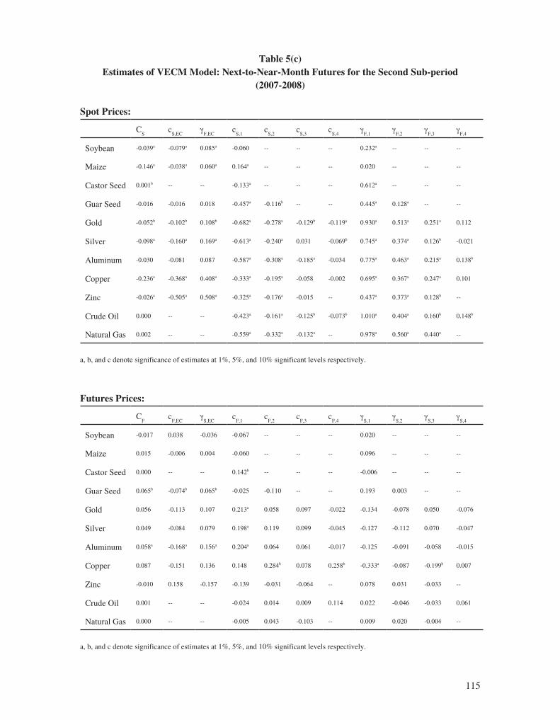
115

Table 5(c) Estimates of VECM Model: Next-to-Near-Month Futures for the Second Sub-period

(2007-2008)

Spot Prices:

CS

cS,EC

γF,EC

cS,1

cS,2

cS,3

cS,4

γF,1

γF,2

γF,3

γF,4

Soybean -0.039a -0.079a 0.085a -0.060 -- -- -- 0.232a -- -- --

Maize -0.146a -0.038a 0.060a 0.164a -- -- -- 0.020 -- -- --

Castor Seed 0.001b -- -- -0.133a -- -- -- 0.612a -- -- --

Guar Seed -0.016 -0.016 0.018 -0.457a -0.116b -- -- 0.445a 0.128a -- --

Gold -0.052b -0.102b 0.108b -0.682a -0.278a -0.129b -0.119a 0.930a 0.513a 0.251a 0.112

Silver -0.098a -0.160a 0.169a -0.613a -0.240a 0.031 -0.069b 0.745a 0.374a 0.126b -0.021

Aluminum -0.030 -0.081 0.087 -0.587a -0.308a -0.185a -0.034 0.775a 0.463a 0.215a 0.138b

Copper -0.236a -0.368a 0.408a -0.333a -0.195a -0.058 -0.002 0.695a 0.367a 0.247a 0.101

Zinc -0.026a -0.505a 0.508a -0.325a -0.176a -0.015 -- 0.437a 0.373a 0.128b --

Crude Oil 0.000 -- -- -0.423a -0.161a -0.125b -0.073b 1.010a 0.404a 0.160b 0.148b

Natural Gas 0.002 -- -- -0.559a -0.332a -0.132a -- 0.978a 0.560a 0.440a --


Futures Prices:

CF

cF,EC

γS,EC

cF,1

cF,2

cF,3

cF,4

γS,1

γS,2

γS,3

γS,4

Soybean -0.017 0.038 -0.036 -0.067 -- -- -- 0.020 -- -- --

Maize 0.015 -0.006 0.004 -0.060 -- -- -- 0.096 -- -- --

Castor Seed 0.000 -- -- 0.142b -- -- -- -0.006 -- -- --

Guar Seed 0.065b -0.074b 0.065b -0.025 -0.110 -- -- 0.193 0.003 -- --

Gold 0.056 -0.113 0.107 0.213a 0.058 0.097 -0.022 -0.134 -0.078 0.050 -0.076

Silver 0.049 -0.084 0.079 0.198a 0.119 0.099 -0.045 -0.127 -0.112 0.070 -0.047

Aluminum 0.058a -0.168a 0.156a 0.204a 0.064 0.061 -0.017 -0.125 -0.091 -0.058 -0.015

Copper 0.087 -0.151 0.136 0.148 0.284b 0.078 0.258b -0.333a -0.087 -0.199b 0.007

Zinc -0.010 0.158 -0.157 -0.139 -0.031 -0.064 -- 0.078 0.031 -0.033 --

Crude Oil 0.001 -- -- -0.024 0.014 0.009 0.114 0.022 -0.046 -0.033 0.061

Natural Gas 0.000 -- -- -0.005 0.043 -0.103 -- 0.009 0.020 -0.004 --


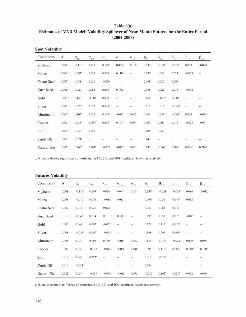
116

Table 6(a) Estimates of VAR Model: Volatility Spillover of Near-Month Futures for the Entire Period

(2004-2008)

Spot Volatility

Commodity A1

α1,1

α1,2

α1,3

α1,4

α1,5

β1,1

β1,2

β1,3

β1,4

β1,5

Soybean 0.004 a -0.110c 0.133 0.110c 0.065 0.182a 0.234 a -0.035 -0.032 0.033 -0.088

Maize 0.004 a 0.082b 0.034 0.060 0.110a -- 0.050c 0.036 0.027 -0.033 --

Castor Seed 0.007 a 0.048 0.036 -0.026 -- -- 0.098a 0.020 0.006 -- --

Guar Seed 0.006 a 0.029 0.061 0.065c 0.132a -- 0.168a 0.022 0.033 -0.032 --

Gold 0.003 a 0.140a -0.002 0.030 -- -- 0.064a 0.155 \a -0.002 -- --

Silver 0.005 a 0.223a 0.033 0.080b -- -- 0.115a 0.019 -0.041a -- --

Aluminum 0.006 a 0.102b 0.021 0.114b -0.022 0.062 0.163a 0.032 -0.062c 0.018 -0.023

Copper 0.002 a 0.233a 0.097a 0.066c 0.167a 0.051 0.060a 0.007 0.018 -0.024 -0.001

Zinc 0.009 a 0.038 0.052 -- -- -- 0.088a 0.052 -- -- --

Crude Oil 0.009 a 0.224a -- -- -- -- 0.047 -- -- -- --

Natural Gas 0.005c 0.265a 0.101b -0.057 -0.062 0.002 0.039 -0.065 0.100c 0.086a 0.214a

a, b , and c denote significance of estimates at 1%, 5%, and 10% significant levels respectively.

Futures Volatility

Commodity A1

α2,1

α2,2

α2,3

α2,4

α2,5

β2,1

Β2,2

β2,3

β2,4

β2,5

Soybean 0.008 a -0.116c 0.103 0.059 0.048 0.104 0.151b -0.058 -0.013 0.086 -0.052

Maize 0.008 a -0.010 0.076 -0.085 0.013 -- 0.093b 0.056 0.145 a 0.052 --

Castor Seed 0.009 a 0.019 0.025 0.028 -- -- 0.030 0.062 0.018 -- --

Guar Seed 0.012 a -0.040 0.034 0.101c 0.145a -- 0.098b 0.052 0.032 -0.027 --

Gold 0.005 a 0.048 0.107c -0.062 -- -- 0.129 a 0.113 a 0.117 a -- --

Silver 0.008 a -0.055 0.107c -0.065 -- -- 0.198 a 0.097 a 0.166 a -- --

Aluminum 0.006 a 0.039 0.050 0.119b -0.017 0.092 0.134 a 0.079c -0.022 0.079c 0.066

Copper 0.008 a 0.040 -0.027 -0.044 -0.026 0.046 0.098 a 0.110 a 0.063c 0.110 a 0.130a

Zinc 0.018 a 0.040 0.257a -- -- -- 0.019 -0.021 -- -- --

Crude Oil 0.016 a -0.023 -- -- -- -- 0.044 -- -- -- --

Natural Gas 0.022 a 0.039 -0.054 -0.075 -0.013 0.075 -0.086c 0.102b 0.121b 0.052 0.009


117

Table 6(b) Estimates of VECM Model:

Near-Month Futures for the First Sub-period (2004-2006)

Spot Volatility

Commodity A1

Α1,1

α1,2

α1,3

α1,4

α1,5

β1,1

β1,2

β1,3

β1,4

β1,5

Soybean 0.003a 0.078 0.037 0.187a 0.109b 0.115b 0.074c 0.030 -0.035 0.026 -0.012

Maize 0.003a 0.120b 0.049 0.083 0.056 0.085 0.130a 0.004 0.033 0.020 -0.024

Castor Seed 0.006a 0.060 0.022 0.003 0.039 -- 0.083c 0.089c -0.018 -0.003 --

Guar Seed 0.010a 0.132a -- -- -- -- 0.130a -- -- -- --

Gold 0.003 0.194a 0.073 0.089c -- -- 0.041 0.039 0.005 -- --

Silver 0.005a 0.236a 0.045 0.003 0.068 -- 0.118a 0.010 -0.094a 0.077b --

Aluminum 0.007a 0.057 0.078 0.160b -- -- 0.140a -0.080 0.043 -- --

Copper 0.004a 0.244a 0.138a 0.166a -- -- 0.024 -0.005 -0.025 -- --

Zinc 0.007a 0.125c -- -- -- -- 0.266a -- -- -- --

Crude Oil 0.010a 0.245a -- -- -- -- 0.015 -- -- -- --

Natural Gas 0.016a 0.253a -- -- -- -- 0.169c -- -- -- --


Futures Volatility

Commodity A1

α2,1

α2,2

α2,3

α2,4

α2,5

β2,1

β2,2

β2,3

β2,4

β2,5

Soybean 0.006a -0.007 0.037 0.094 -0.001 -0.009 0.044 0.026 -0.012 0.103b 0.068

Maize 0.004a -0.014 0.032 -0.215a 0.094 0.029 0.134a 0.127b 0.157a 0.094c 0.191a

Castor Seed 0.007a -0.055 0.086 0.004 -0.003 0.036 0.103c 0.080 -0.031 --

Guar Seed 0.015a 0.164a -- -- -- -- 0.091b -- -- -- --

Gold 0.005a 0.172b 0.048 -0.074 -- -- 0.153a 0.029 0.181a -- --

Silver 0.005a 0.155b 0.144c -0.134c 0.036 -- 0.197a 0.064 0.125b 0.111b --

Aluminum 0.007a 0.060 0.100 0.191b -- -- 0.204a -0.001 0.114 -- --

Copper 0.010a 0.050 -0.116 0.067 -- -- 0.065 0.109b 0.146a -- --

Zinc 0.021a -0.064 -- -- -- -- 0.106 -- -- -- --

Crude Oil 0.016a -0.015 -- -- -- -- -0.019 -- -- -- --

Natural Gas 0.037a -0.063 -- -- -- -- -0.064 -- -- -- --

a, b, and c denotes significance of estimates at 1%, 5%, and 10% significant levels respectively.

118

Table 6(c) Estimates of VECM Model:

Near-Month Futures for the Second Sub-period (2007-2008)

Spot Volatility

Commodity A1

Α1,1

α1,2

α1,3

α1,4

α1,5

β1,1

β1,2

β1,3

β1,4

β1,5

Soybean 0.005a -0.011 0.227a -- -- -- 0.219a -0.022 -- -- --

Maize 0.005a 0.118b -- -- -- -- 0.019 -- -- -- --

Castor Seed 0.007a 0.040 -- -- -- -- 0.137b -- -- -- --

Guar Seed 0.007a 0.069 -- -- -- -- 0.075b -- -- -- --

Gold 0.004a 0.003 -0.015 -- -- -- 0.113a 0.135a -- -- --

Silver 0.003a 0.103b 0.034 0.164a -- -- 0.136a 0.036 -0.008 -- --

Aluminum 0.005a 0.102b 0.052 -- -- -- 0.067c 0.097a -- -- --

Copper 0.001 0.124a 0.128a -0.032 0.059 -0.047 0.056b -0.014 0.105a 0.007 0.089a

Zinc 0.011a 0.035 -- -- -- -- -0.004 -- -- -- --

Crude Oil 0.006a 0.176a 0.104b -- -- -- 0.065c 0.023 -- -- --

Natural Gas 0.011a 0.080 0.103 -- -- -- 0.017 -0.059 -- -- --


Futures Volatility

Commodity A2

α2,1

Α2,2

α2,3

α2,4

α2,5

β2,1

β2,2

β2,3

β2,4

β2,5

Soybean 0.009a 0.052 0.210 0.086 -0.009 -- -- --

Maize 0.010a 0.118 -- -- -- -- 0.066 -- -- -- --

Castor Seed 0.011a -0.056 -- -- -- -- 0.002 -- -- -- --

Guar Seed 0.014a 0.070 -- -- -- -- -0.074 -- -- -- --

Gold 0.007a 0.001 0.042 -- -- -- 0.084c 0.139a -- -- --

Silver 0.010a 0.020 -0.045 0.054 -- -- 0.100b 0.119b 0.071 -- --

Aluminum 0.009a -0.007 0.078 -- -- -- 0.035 0.099c -- -- --

Copper 0.008a -0.139 0.109 -0.064 -0.089 0.275a 0.059 0.138a -0.041 0.162a 0.175a

Zinc 0.017a 0.170b -- -- -- -- 0.059 -- -- -- --

Crude Oil 0.017a 0.023 -0.095 -- -- -- 0.016 -0.004 -- -- --

Natural Gas 0.024a 0.109 0.067 -- -- -- -0.093c -0.085 -- -- --


119

Table 7(a) Estimates of VAR Model: Next-to-Near-Month Futures for the Entire Period (2004-2008)

Spot Volatility

Commodity A1

α1,1

α1,2

Α1,3

α1,4

α1,5

β1,1

β1,2

β1,3

β1,4

β1,5

Soybean 0.003a -0.029 0.102a 0.148a 0.148a 0.174a 0.202a 0.028 -0.048 0.009 -0.090b

Maize 0.005a 0.138a 0.054 0.061 0.111a -- 0.012 -0.002 0.045c -0.051 --

Castor Seed 0.007a 0.039 0.037 -- -- -- 0.109a 0.010 -- -- --

Guar Seed 0.005a 0.004 0.105a 0.075b 0.112a -- 0.154a 0.006 0.031 -0.025 --

Gold 0.003a 0.097a -0.007 0.028 -- -- 0.076a 0.161a 0.019 -- --

Silver 0.005a 0.215a 0.034 0.078b -- -- 0.112a 0.016 -0.043b -- --

Aluminum 0.006 0.063 0.011 0.087c 0.005 0.080 0.178a 0.069c -0.039 0.034 -0.026

Copper 0.003a 0.287a 0.083b 0.080b 0.119a 0.043 0.090a 0.000 0.009 -0.040c -0.009

Zinc 0.010a 0.045 0.051 -- -- -- 0.118a 0.056 -- -- --

Crude Oil 0.009a 0.200a -- -- -- -- 0.044 -- -- -- --

Natural Gas 0.004 0.322a 0.064 -0.054 0.048 -0.008 0.241a -0.072 0.095 -0.013 0.191a


Futures Volatility

Commodity A1

α2,1

α2,2

α2,3

α2,4

α2,5

β2,1

β2,2

β2,3

β2,4

β2,5

Soybean 0.007a -0.051 0.042 0.019 0.021 0.023 0.137a 0.017 0.046 0.095b 0.020

Maize 0.009a -0.007 0.033 -0.032 0.068 -- 0.058 0.101a 0.075c 0.031 --

Castor Seed 0.010a -0.014 -0.014 -- -- -- 0.052 0.092b -- -- --

Guar Seed 0.013a -0.092 0.046 0.071 0.133a -- 0.116a 0.039 0.048 -0.004

Gold 0.005a 0.074 0.075 -0.067 -- -- 0.135a 0.123a 0.112a -- --

Silver 0.008a -0.047 0.019 -0.044 -- -- 0.192a 0.112a 0.176a -- --

Aluminum 0.005a 0.079 -0.079 0.116b -0.013 0.136a 0.102b 0.104b 0.057 0.142a 0.016

Copper 0.008a 0.075 -0.091c -0.009 -0.025 0.021 0.102a 0.116a 0.079b 0.122a 0.117a

Zinc 0.017a 0.012 0.249a -- -- -- 0.031 -0.013 -- -- --

Crude Oil 0.014a -0.022 -- -- -- -- 0.063c -- -- -- --

Natural Gas 0.020a 0.014 -0.043 -0.035 -0.001 0.049 -0.057 0.113b 0.085c -0.006 0.016


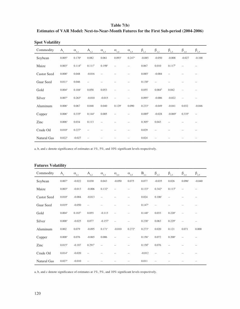
120

Table 7(b) Estimates of VAR Model: Next-to-Near-Month Futures for the First Sub-period (2004-2006)

Spot Volatility

Commodity A1

α1,1

Α1,2

α1,3

α1,4

α1,5

β1,1

β1,2

β1,3

β1,4

β1,5

Soybean 0.005a 0.170a 0.082 0.061 0.093c 0.247a -0.085 -0.050 -0.008 -0.027 -0.100

Maize 0.003a 0.114b 0.111b 0.198a -- -- 0.067 0.010 0.117b -- --

Castor Seed 0.008a 0.048 -0.016 -- -- -- 0.085c -0.004 -- -- --

Guar Seed 0.011a 0.046 -- -- -- -- 0.130a -- -- -- --

Gold 0.004a 0.104c 0.058 0.053 -- -- 0.055 0.084b 0.042 -- --

Silver 0.007a 0.263a -0.010 -0.015 -- -- 0.095a -0.006 -0.022 -- --

Aluminum 0.006a 0.067 0.048 0.040 0.129c 0.090 0.233a -0.049 -0.041 0.032 -0.046

Copper 0.006a 0.335a 0.144a 0.005 -- -- 0.089b -0.028 -0.069c 0.335a --

Zinc 0.006a 0.034 0.113 -- -- -- 0.305a 0.043 -- -- --

Crude Oil 0.010a 0.227a -- -- -- -- 0.029 -- -- -- --

Natural Gas 0.022a -0.027 -- -- -- -- 0.024 -- -- -- --


Futures Volatility

Commodity A2

α2,1

Α2,2

α2,3

α2,4

α2,5

Β2,1

β2,2

β2,3

β2,4

β2,5

Soybean 0.007a -0.022 0.030 0.043 -0.050 0.075 0.077 -0.035 0.026 0.096c -0.040

Maize 0.003a -0.013 -0.006 0.132a -- -- 0.133a 0.342a 0.113b -- --

Castor Seed 0.010a -0.004 -0.013 -- -- -- 0.024 0.106c -- -- --

Guar Seed 0.019a -0.050 -- -- -- -- 0.147a -- -- -- --

Gold 0.004a 0.183b 0.055 -0.113 -- -- 0.148a 0.033 0.220a -- --

Silver 0.008a -0.025 0.077 -0.157c -- -- 0.238a 0.063 0.229a -- --

Aluminum 0.002 0.079 -0.095 0.171c -0.010 0.272a 0.273a 0.020 0.121 0.071 0.000

Copper 0.008a 0.076 -0.065 0.006 -- -- 0.156a 0.072 0.200a -- --

Zinc 0.015a -0.187 0.291b -- -- -- 0.158b 0.076 -- -- --

Crude Oil 0.014a -0.020 -- -- -- -- -0.012 -- -- -- --

Natural Gas 0.027a -0.010 -- -- -- -- 0.011 -- -- -- --


121

Table 7(c) Estimates of VAR Model: Next-to-Near-Month Futures for the Second Sub-period (2007-2008)

Spot Volatility

Commodity A1

α1,1

Α1,2

Α1,3

α1,4

α1,5

β1,1

β1,2

β1,3

β1,4

β1,5

Soybean 0.005a -0.065 0.131b -- -- -- 0.299a 0.091 -- -- --

Maize 0.005a 0.105c -- -- -- -- 0.008 -- -- -- --

Castor Seed 0.003a -0.003 0.026 -0.080 -0.058 -0.043 0.068 0.056 0.137b 0.042 0.230a

Guar Seed 0.007a 0.083 -- -- -- -- 0.051 -- -- -- --

Gold 0.003a 0.046 -0.015 -- -- -- 0.116a 0.146a -- -- --

Silver 0.003a 0.086c 0.048 0.213a -- -- 0.171a 0.030 -0.041 -- --

Aluminum 0.007a 0.057 0.030 -- -- -- 0.089c 0.086c -- -- --

Copper 0.001a 0.189a 0.070 -0.037 0.079c -0.019 0.091a 0.023 0.027 0.040 0.045c

Zinc 0.011a 0.069 0.060 -- -- -- -0.017 0.030 -- -- --

Crude Oil 0.007a 0.136a -- -- -- -- 0.119a -- -- -- --

Natural Gas 0.011a 0.376a -- -- -- -- 0.055 -- -- -- --


Futures Volatility

Commodity A2

α2,1

Α2,2

α2,3

α2,4

α2,5

β2,1

β2,2

β2,3

β2,4

β2,5

Soybean 0.011a -0.018 0.108b -- -- -- 0.130b 0.010 -- -- --

Maize 0.014a -0.076 -- -- -- -- 0.046 -- -- -- --

Castor Seed 0.005a 0.043 0.006 0.067 0.156a -0.036 -0.074 0.110b 0.120b 0.018 0.169a

Guar Seed 0.015a 0.063 -- -- -- -- -0.078 -- -- -- --

Gold 0.006a 0.037 0.034 -- -- -- 0.083c 0.156a -- -- --

Silver 0.009a -0.011 -0.070 0.085 -- -- 0.142a 0.126b 0.068 -- --

Aluminum 0.010a 0.116c -0.038 -- -- -- 0.005 0.064 -- -- --

Copper 0.007a -0.132 0.003 -0.117 -0.080 0.279a 0.118a 0.191a -0.044 0.166a 0.164a

Zinc 0.018a 0.108 0.145c -- -- -- -0.044 -0.006 -- -- --

Crude Oil 0.013a 0.010 -- -- -- -- 0.095b -- -- -- --

Natural Gas 0.020a -0.013 -- -- -- -- -0.060 -- -- -- --


price discovery in emerging commodity markets: spot and ... · 79 price discovery in emerging...

Documents