price discovery in commodity markets: a study of...

International Journal of Multidisciplinary Research and Modern Education (IJMRME)

ISSN (Online): 2454 - 6119

(www.rdmodernresearch.com) Volume II, Issue II, 2016

571

PRICE DISCOVERY IN COMMODITY MARKETS: A STUDY OF PRECIOUS METALS MARKET IN

MULTI COMMODITY EXCHANGE Dr. S. Nirmala* & K. Deepthy**

* Research Supervisor, Associate Professor, Department of Business Administration & Principal, PSGR Krishnammal College for Women, Peelamedu,

Coimbatore, Tamilnadu ** Ph.D Research Scholar, Department of Business Administration, PSGR Krishnammal

College for Women, Peelamedu, Coimbatore, Tamilnadu Abstract: The study analyses price discovery function of Gold and Silver market of MCX for the period 01/01/2014 to 31/10/2016. After identifying single co integrating vector, VECM is used to analyze long run and short run causality among these commodities. The evidence shows that for gold there is a unidirectional causal relationship from future to spot market in long run, while there is a bidirectional relationship in short run. In the case of silver, there is a bidirectional causal relationship between spot and futures in long run, and a unidirectional relationship from futures to spot in short run. Key Words: Price Discovery, Precious Metals, Cointegration, VECM, Wald Test & Granger Causality Introduction: Some metals because of their scarcity in nature are classified as Precious Metals. Historically, they are considered as a form of currency. Today, they are regarded as an investment and an industrial commodity. Precious metals like Gold, Silver, Platinum and palladium still possess ISO 4217 currency code, which indicates that they are not just currency but de facto money. Owing to the limited bullion supplies, the demand is largely met through imports. (Source: MCX India) Gold is the most sought after of all precious metals, is acquired throughout the world for its beauty, liquidity, investment qualities and industrial properties. India consumes about 800 MT of gold which accounts to about 20% of gold consumption globally. More than 50% of this is used for making gold jwellery. (Source: http:// business.mapsofindia.com/india-market/gold.html#sthash.UH0A4Dpp.dpuf) As an investment vehicle, gold is typically viewed as a financial asset, which maintains its value and purchasing power during inflationary periods. India’s demand for gold jewelry in quarter 3 of 2016 reached to 493 tons. The demand for gold for investment purposes amounted to approximately 448.4 metric tons in Q2 2016. (Source: economic times) Silver has been used by man for thousands of years and in ancient times, it was second most valuable precious metal with gold being the highest. Silver is used traditionally to make jewelry, ornaments, silverware, tableware and coins. Modern Science also discovered uses of silver in manufacture of mirrors, clothing, electrical circuitry, photography, dentistry and medical uses. Silver is prized primarily for its dual role as monetary asset as well as an industrial metal utilized in wide range of existing and growing application. Price Discovery is the process through which markets attempt to reach equilibrium prices. In the static sense, price discovery implies existence of equilibrium prices. In the dynamic sense, price discovery process describes how information is produced and transmitted across the market (Leatham & Yang, 1999). Price discovery is an important function of commodity market. A market with highest price discovery is


ISSN (Online): 2454 - 6119


572

most likely to trade fastest, given a common commodity shock, and thus provide highest level of pricing guidance to market entities that trade slower and thus get a high proportion of their information from leading markets. (Ivanov & Jose, 2011) In this regard, the present study has been undertaken to examine price discovery process of precious metals market. Review of Literature: (Easwaran & Ramasundaram, 2008)studied whether there is efficient price discovery in 4 agricultural commodities viz., Castor, Cotton, Pepper and Soya. It was found that there is no price discovery in the sample market and that the sample market is inefficient. The results indicated that futures market failed in hedge against volatile prices. (N. Kumar & Arora, 2011) studied the price discovery of gold traded in MCX through Augmented Dickey Fuller test, Johansen’s Cointegration test and Granger Causality test. In the study closing prices of futures and spot price of gold are taken into account for a period of June 2005 – December 2009. From the analysis, it has been found that futures market is performing the price discovery process. (Ivanov & Jose, 2011)examined the relative price discovery between futures and cash prices in 30 Indices and commodity markets based on Gonzalo and Grauper permanent transitory methodology. With exception of feeder cattle and Wheat Minneapolis, the price discovery is occurring in futures market. A cross section of variability of Informational shares reveals that information share of futures market is lower when trading volume is lower or if the commodity is an energy commodity or agricultural commodity or if it has traded in ETF. (Srinivasan & Ibrahim, 2012) studied the Price Discovery and Asymmetric Volatility Spillovers in Indian Spot-Futures Gold Markets in NCDEX. The study revealed that there is long run equilibrium relationship between spot and futures prices. The study states that spot prices perform the price discovery function. A Bivariate ECM-EGARCH (1, 1) model is applied to find out the volatility spillovers between the markets. The study revealed that Significant volatility spill over exists between the markets but spillovers from spot to futures are more significant than the reverse direction, which means that the information flow from spot to futures is stronger. Objective of the Study: To analyze the price discovery process of Gold future and spot price contracts To analyze the price discovery process of Silver future and spot price contracts

Research Methodology: The study is based on secondary data. Secondary data of futures and spot price of

gold and silver are collected from 01/01/2014 to 31/10/2016. All the data are obtained from MCX Website. The analysis has been done through Eviews7 software. The study used Augmented Dickey Fuller test (ADF Test) to check the stationarity of data. The long-term relationship between futures and spot price is found out using Cointegration technique. Weak exogeneity test is applied to find out the speed of adjustment of prices towards equilibrium relationship. Short run integration between Spot and futures market are analyzed through Vector Error Correction Model (VECM). The granger causality test is applied to examine the lead lag relationship between spot and futures market. Augmented Dickey Fuller Test:

Before testing for cointegration, the time series must be checked for stationarity. The stationarity properties and exhibition of unit roots in the time series are substantiated by performing Augmented Dickey Fuller tests. This test is conducted on the variables in original price series and first differences. The variables that are


ISSN (Online): 2454 - 6119


573

integrated in the same order may be cointegrated, while the unit root tests find out which variables are integrated of same order, for example; if integrated by order one, the it is denoted as 1(1). The following ADF regression equation is used for testing stationarity,

△Yt = β1 + β2t +δYt-1+αi 𝑚𝑖−1 △Yt-1+ut …….(1)

Where, Yt is a vector to be tested for cointegration, t is the time or trend variable, △Yt, is then first order difference i.e; ( Yt – Yt-1 ) and ut is the pure white noise error term. The null hypothesis that, δ=0, signifying unit root, states that the time series is non-stationary while, the alternative hypothesis, δ<0 signifies that the time series is stationary, thereby rejecting the null hypothesis.(Kar, C, & Jha, 2013)

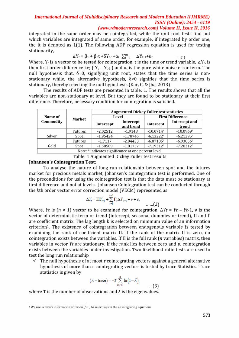
The results of ADF tests are presented in table: 1. The results shows that all the variables are non-stationary at level. But they are found to be stationary at their first difference. Therefore, necessary condition for cointegration is satisfied.

Table: 1 Augmented Dickey Fuller test results Johansen’s Cointegration Test:

To analyse the nature of long-run relationship between spot and the futures market for precious metals market, Johansen’s cointegration test is performed. One of the preconditions for using the cointegration test is that the data must be stationary at first difference and not at levels. Johansen Cointegration test can be conducted through the kth order vector error correction model (VECM) represented as

……(2) Where, Yt is (n × 1) vector to be examined for cointegration, ΔYt = Yt – Yt-1, ν is the vector of deterministic term or trend (intercept, seasonal dummies or trend), П and Ѓ are coefficient matrix. The lag length k is selected on minimum value of an information criterion1. The existence of cointegration between endogenous variable is tested by examining the rank of coefficient matrix П. If the rank of the matrix П is zero, no cointegration exists between the variables. If П is the full rank (n variables) matrix, then variables in vector Yt are stationary. If the rank lies between zero and p, cointegration exists between the variables under investigation. Two likelihood ratio tests are used to test the long run relationship The null hypothesis of at most r cointegrating vectors against a general alternative

hypothesis of more than r cointegrating vectors is tested by trace Statistics. Trace statistics is given by

….(3) where T is the number of observations and λ is the eigenvalues.

1 We use Schwarz information criterion (SIC) to select lags in the co integrating equations

Name of Commodity

Market

Augmented Dickey Fuller test statistics Level First Difference

Intercept Intercept and trend

Intercept Intercept and

trend

Silver

Futures -2.02512 -1.9148 -10.0714* -10.0969*

Spot -1.95424 -1.78745 -6.13222* -6.21295*

Gold

Futures -1.7117 -2.04433 -6.87105* -6.93856*

Spot -1.58589 -1.81757 -7.19312* -7.28312*

Note: * indicates significance at one percent level


ISSN (Online): 2454 - 6119


574

The null hypothesis of r cointegrating vector against the alternative of r + 1 is tested by Maximum Eigen value statistic Maximum Eigen Value is given by

……(4) In our test for the cointegration between Precious metal futures and spot market, n = 2 and null hypothesis would be rank = 0 and alternative hypothesis would be rank = 1. If rank = 0 existence of cointegration is rejected and r = 1 is existence of cointegration not rejected, we conclude that the two series are cointegrated. However, if rank = 0 is not rejected, we conclude that the two series are not cointegrated.(B. Kumar & Pandey, 2011)

The results of cointegration tests are presented in the table 2. The results reveal that there is at most 1 cointegrating equation between the variables. Both trace statistics and maximum Eigen values support the presence of cointegration. So, it has been concluded that there is long run equilibrium relationship between spot and future of gold and silver.

Table 2: Johansen’s Cointegration test results

Name of Commodity Vector

(r) Trace statistics

(λtrace) Max-Eigen Statistics

(λ max)

Silver (Lag length 2 as per SC: Schwarz information criterion)

H0: r=0 117.6852* 113.9210* H1:r≥1 3.764198 3.764198

Gold (Lag length 3, as per SC: Schwarz information criterion)

(Lag length 3, as per

H0: r=0 33.64551* 31.13482*

H1:r≥1 2.510684 2.510684

Note: * indicates significance at one percent level

Vector Error Correction Model (VECM): The cointegration criterion, if validated, facilitates the error correction model.

The model has been used to identify the market where price discovery occurs. The VECM is estimated by putting to use an Ordinary Least Square (OLS) in each equation.

…..(5) where ΔSt is the change in spot price, measured by the RHS (i.e.) as,i and bs,i being the coefficients of lagged spot prices (denoted by ΔSt–i) and lagged futures prices (denoted by ΔFt–i), respectively,as,0 is deterministic and S,t is the error term, while the lag is denoted by i. With the above explanatory equation, the VECM for two time series sets (in the current case spot and futures data series) can be examined. (Prasanna, 2014)

Table 3: Vector Error Correction Model Results Coefficient Std. Error t-Statistic Prob Inference

Gold (Dependent variable:

Spot price) C (1) -0.082757 0.022930 -3.609131 0.0003

F S Gold

(Dependent variable: Future price)

C (1) -0.055007 0.032301 -1.702916 0.0890

Silver (Dependent variable: Spot price)

C (1) -0.327294 0.040190 -8.143698 0.0000 F S

Gold (Dependent variable: Future price)

C (1) -0.148634 0.054601 -2.722195 0.0066

From the above table it can be seen that the error term for gold where spot price is the dependent variable have a negative sign and it is significant. On the other hand, error correction term for gold, where future price is dependent variable also has a


ISSN (Online): 2454 - 6119


575

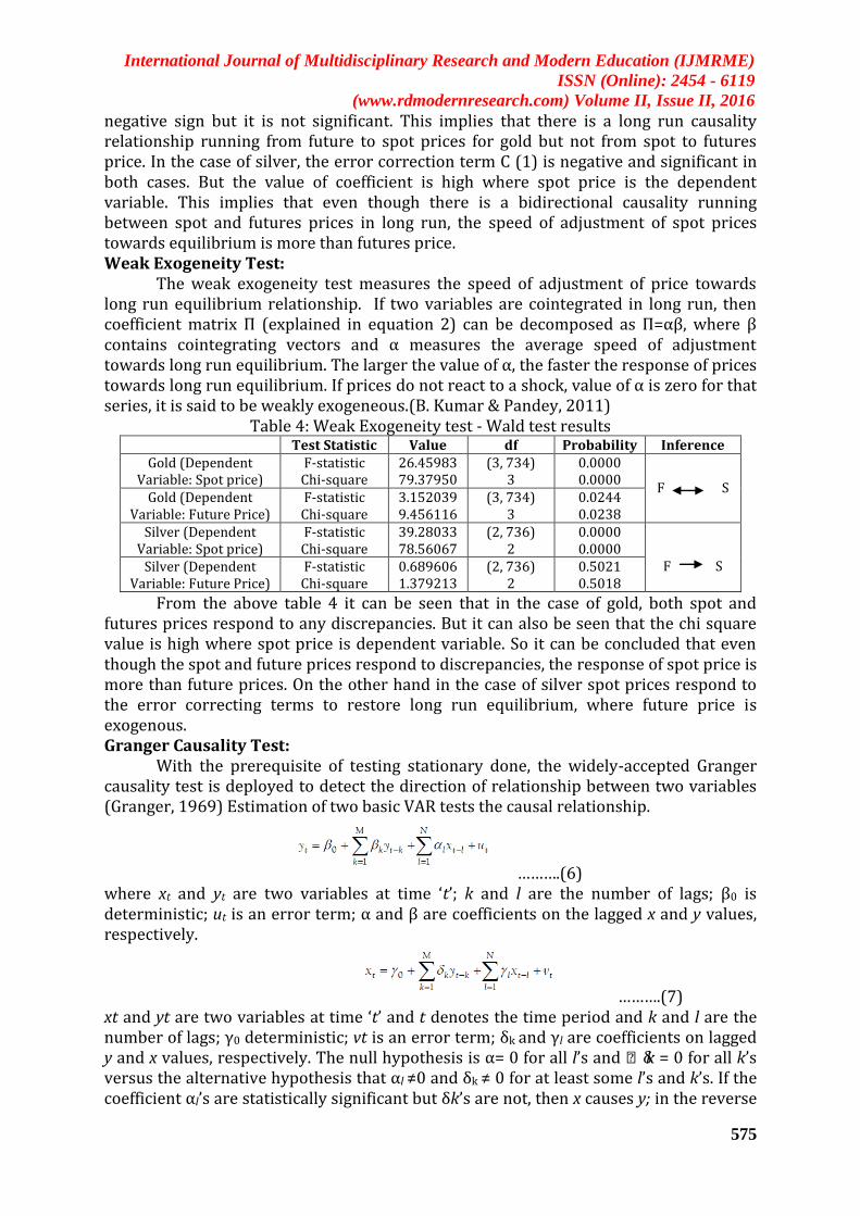
negative sign but it is not significant. This implies that there is a long run causality relationship running from future to spot prices for gold but not from spot to futures price. In the case of silver, the error correction term C (1) is negative and significant in both cases. But the value of coefficient is high where spot price is the dependent variable. This implies that even though there is a bidirectional causality running between spot and futures prices in long run, the speed of adjustment of spot prices towards equilibrium is more than futures price. Weak Exogeneity Test:

The weak exogeneity test measures the speed of adjustment of price towards long run equilibrium relationship. If two variables are cointegrated in long run, then coefficient matrix Π (explained in equation 2) can be decomposed as Π=αβ, where β contains cointegrating vectors and α measures the average speed of adjustment towards long run equilibrium. The larger the value of α, the faster the response of prices towards long run equilibrium. If prices do not react to a shock, value of α is zero for that series, it is said to be weakly exogeneous.(B. Kumar & Pandey, 2011)

Table 4: Weak Exogeneity test - Wald test results Test Statistic Value df Probability Inference

Gold (Dependent Variable: Spot price)

F-statistic Chi-square

26.45983 79.37950

(3, 734) 3

0.0000 0.0000

F S Gold (Dependent

Variable: Future Price) F-statistic Chi-square

3.152039 9.456116

(3, 734) 3

0.0244 0.0238

Silver (Dependent Variable: Spot price)


39.28033 78.56067

(2, 736) 2

0.0000 0.0000

F S Silver (Dependent Variable: Future Price)


0.689606 1.379213

(2, 736) 2

0.5021 0.5018

From the above table 4 it can be seen that in the case of gold, both spot and futures prices respond to any discrepancies. But it can also be seen that the chi square value is high where spot price is dependent variable. So it can be concluded that even though the spot and future prices respond to discrepancies, the response of spot price is more than future prices. On the other hand in the case of silver spot prices respond to the error correcting terms to restore long run equilibrium, where future price is exogenous. Granger Causality Test:

With the prerequisite of testing stationary done, the widely-accepted Granger causality test is deployed to detect the direction of relationship between two variables (Granger, 1969) Estimation of two basic VAR tests the causal relationship.

……….(6) where xt and yt are two variables at time ‘t’; k and l are the number of lags; β0 is deterministic; ut is an error term; α and β are coefficients on the lagged x and y values, respectively.

……….(7) xt and yt are two variables at time ‘t’ and t denotes the time period and k and l are the number of lags; γ0 deterministic; vt is an error term; δk and γl are coefficients on lagged y and x values, respectively. The null hypothesis is α= 0 for all l’s and δk = 0 for all k’s versus the alternative hypothesis that αl ≠0 and δk ≠ 0 for at least some l’s and k’s. If the coefficient αl’s are statistically significant but δk’s are not, then x causes y; in the reverse


ISSN (Online): 2454 - 6119


576

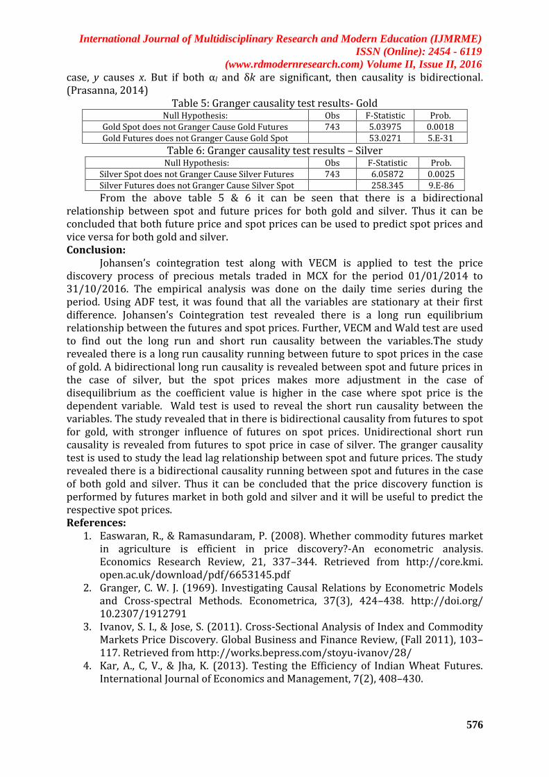
case, y causes x. But if both αl and δk are significant, then causality is bidirectional. (Prasanna, 2014)

Table 5: Granger causality test results- Gold Null Hypothesis: Obs F-Statistic Prob.

Gold Spot does not Granger Cause Gold Futures 743 5.03975 0.0018 Gold Futures does not Granger Cause Gold Spot 53.0271 5.E-31

Table 6: Granger causality test results – Silver Null Hypothesis: Obs F-Statistic Prob.

Silver Spot does not Granger Cause Silver Futures 743 6.05872 0.0025 Silver Futures does not Granger Cause Silver Spot 258.345 9.E-86

From the above table 5 & 6 it can be seen that there is a bidirectional relationship between spot and future prices for both gold and silver. Thus it can be concluded that both future price and spot prices can be used to predict spot prices and vice versa for both gold and silver. Conclusion:

Johansen’s cointegration test along with VECM is applied to test the price discovery process of precious metals traded in MCX for the period 01/01/2014 to 31/10/2016. The empirical analysis was done on the daily time series during the period. Using ADF test, it was found that all the variables are stationary at their first difference. Johansen’s Cointegration test revealed there is a long run equilibrium relationship between the futures and spot prices. Further, VECM and Wald test are used to find out the long run and short run causality between the variables.The study revealed there is a long run causality running between future to spot prices in the case of gold. A bidirectional long run causality is revealed between spot and future prices in the case of silver, but the spot prices makes more adjustment in the case of disequilibrium as the coefficient value is higher in the case where spot price is the dependent variable. Wald test is used to reveal the short run causality between the variables. The study revealed that in there is bidirectional causality from futures to spot for gold, with stronger influence of futures on spot prices. Unidirectional short run causality is revealed from futures to spot price in case of silver. The granger causality test is used to study the lead lag relationship between spot and future prices. The study revealed there is a bidirectional causality running between spot and futures in the case of both gold and silver. Thus it can be concluded that the price discovery function is performed by futures market in both gold and silver and it will be useful to predict the respective spot prices. References:

1. Easwaran, R., & Ramasundaram, P. (2008). Whether commodity futures market in agriculture is efficient in price discovery?-An econometric analysis. Economics Research Review, 21, 337–344. Retrieved from http://core.kmi. open.ac.uk/download/pdf/6653145.pdf

2. Granger, C. W. J. (1969). Investigating Causal Relations by Econometric Models and Cross-spectral Methods. Econometrica, 37(3), 424–438. http://doi.org/ 10.2307/1912791

3. Ivanov, S. I., & Jose, S. (2011). Cross-Sectional Analysis of Index and Commodity Markets Price Discovery. Global Business and Finance Review, (Fall 2011), 103–117. Retrieved from http://works.bepress.com/stoyu-ivanov/28/

4. Kar, A., C, V., & Jha, K. (2013). Testing the Efficiency of Indian Wheat Futures. International Journal of Economics and Management, 7(2), 408–430.


ISSN (Online): 2454 - 6119


577

5. Kumar, B., & Pandey, A. (2011). International Linkages of the Indian Commodity Futures Markets. Modern Economy, 2(July), 213–227. http://doi.org/10.4236 /me.2011.23027

6. Kumar, N., & Arora, S. (2011). Price Discovery in Precious Metals Market : A Study of Gold. International Journal of Financial Management, 1(1), 70–82.

7. Leatham, J., & Yang, J. (1999). Price Discovery in Wheat Futures Markets. Journal of Agricultural and Applied Economics, 2(August), 359–370. http://doi.org/ 10.1017/S1074070800008634

8. Prasanna, G. R. S. (2014). Performance Evaluation of Agricultural Commodity Futures Market in India. IUP Journal of Applied Finance, 20(1), 34–45. Retrieved from http://search.ebscohost.com/login.aspx?direct=true&db=buh&AN=9508 7521&site=ehost-live

9. Srinivasan, P., & Ibrahim, P. (2012). Price Discovery and Asymmetric Volatility Spillovers in Indian Spot-Futures Gold Markets International Journal of Economic Sciences and Applied Research, 5(3), 65–80.

10. www.mcxindia.com 11. www.economictimes.com

http://search.ebscohost.com/login.aspx?direct=true&db=buh&AN=9508

price discovery in commodity markets: a study of...

Documents