presentation for the 19th eurostar users conference june 2011

Consider Covariance Analysis Monte Carlo and Collocation

withOR.A.SI – (Orbit and Attitude Simulator)

Antonios Arkas Flight Dynamics Engineer

-0,0004 -0,0002 0,0000 0,0002 0,0004

-0,0004

-0,0002

0,0000

0,0002

0,0004

ey

ex

1. Advances in OR.A.SI

Consider Covariance Analysis - Monte Carlo and Collocation with

OR.A.SI (Orbit and Attitude Simulator)

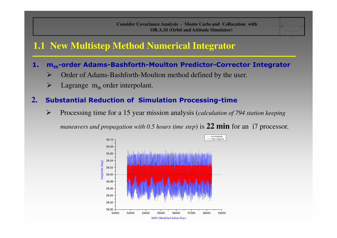
1.1 New Multistep Method Numerical Integrator

1. mth-order Adams-Bashforth-Moulton Predictor-Corrector Integrator

� Order of Adams-Bashforth-Moulton method defined by the user.

� Lagrange mth order interpolant.

2. Substantial Reduction of Simulation Processing-time

� Processing time for a 15 year mission analysis (calculation of 794 station keeping

maneuvers and propagation with 0.5 hours time step) is 22 min for an i7 processor.

52000 53000 54000 55000 56000 57000 58000 59000

38,90

38,92

38,94

38,96

38,98

39,00

39,02

39,04

39,06

39,08

39,10

true longitude

mean longitude

longit

ude

[deg

]

MJD (Modified Julian Day)



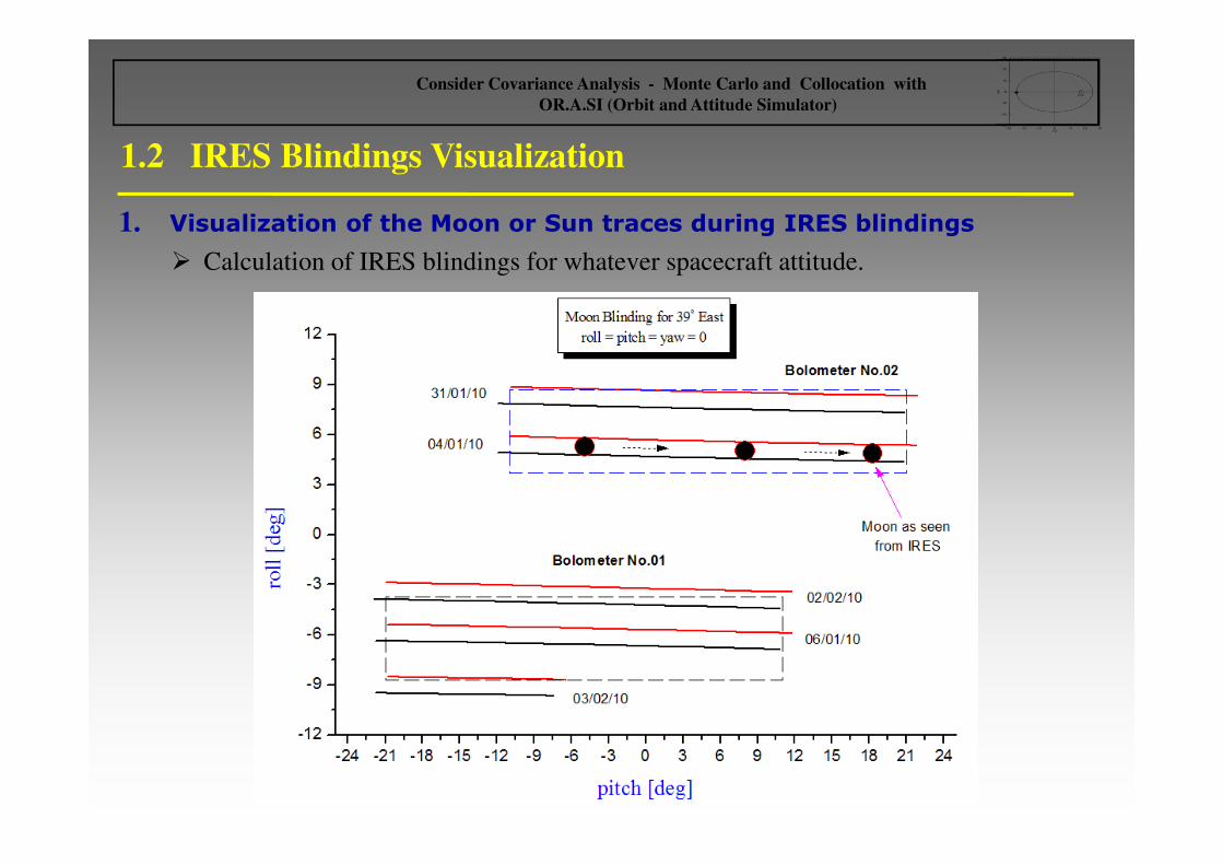
1.2 IRES Blindings Visualization

1. Visualization of the Moon or Sun traces during IRES blindings

� Calculation of IRES blindings for whatever spacecraft attitude.



1.3 Relocation Maneuvers Calculation for GEO Spacecrafts

1. Relocation Module Characteristics

� Calculation of velocity increments corresponding to drift setting and drift stop

maneuvers each one of which is performed by means of two tangential maneuvers.

� Manual setting of first drift setting and last drift stop maneuver epochs i.e.

adjustment of the drift phase duration and control of the relevant propellant

consumption.

� Epoch calculation for the second drift setting maneuver and the first drift stop

maneuver.

� Automatic or manual setting of mean eccentricity during drift phase.

� Plotting of achievable area for mean eccentricity vector during the drift phase.

� Flexibility to choose a specific orbit, for a desired epoch following the last drift

stop maneuver, or initialize a station keeping cycle with desired characteristics (if

reachable).



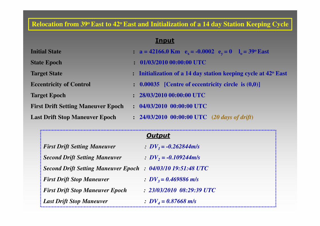
Relocation from 39o East to 42o East and Initialization of a 14 day Station Keeping Cycle

Input

Initial State : a = 42166.0 Km ex = -0.0002 ey = 0 lo = 39o East

State Epoch : 01/03/2010 00:00:00 UTC

Target State : Initialization of a 14 day station keeping cycle at 42o East

Eccentricity of Control : 0.00035 [Centre of eccentricity circle is (0,0)]

Target Epoch : 28/03/2010 00:00:00 UTC

First Drift Setting Maneuver Epoch : 04/03/2010 00:00:00 UTC

Last Drift Stop Maneuver Epoch : 24/03/2010 00:00:00 UTC (20 days of drift)

Output

First Drift Setting Maneuver : DV1 = -0.262844m/s

Second Drift Setting Maneuver : DV2 = -0.109244m/s

Second Drift Setting Maneuver Epoch : 04/03/10 19:51:48 UTC

First Drift Stop Maneuver : DV3 = 0.469886 m/s

First Drift Stop Maneuver Epoch : 23/03/2010 08:29:39 UTC

Last Drift Stop Maneuver : DV4 = 0.87668 m/s

Relocation from 39o East to 42o East – Longitude Evolution

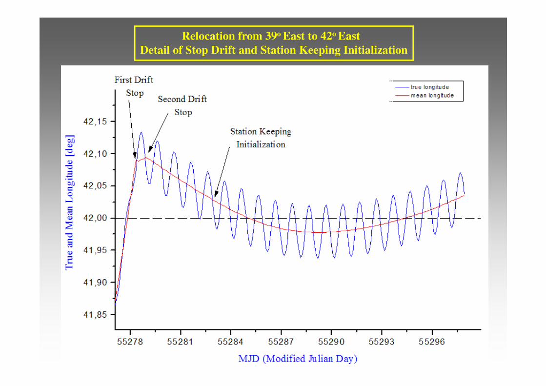
Relocation from 39o East to 42o East

Detail of Stop Drift and Station Keeping Initialization

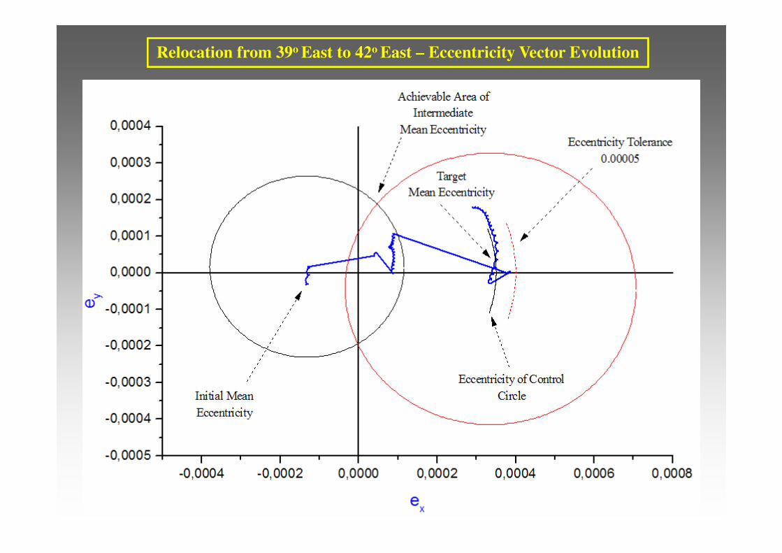
Relocation from 39o East to 42o East – Eccentricity Vector Evolution

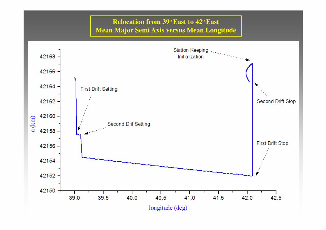
Relocation from 39o East to 42o East

Mean Major Semi Axis versus Mean Longitude

1.4 Theoretical Longitude Window Breakdown (1/2)

1. Input Data

� Station keeping cycle duration. (14 days)

� Nominal longitude. (39o East)

� Longitude window semi dimension. (0.09o)

� Eccentricity of control. (0.0004)

� Time interval between N/S and E/W maneuvers. (2.5 days)

� Mean value of normal velocity increment during N/S maneuvers. (2.0 m/s)

� True longitude 3σ orbit determination error. (0.004o)

� Major semi axis 3σ orbit determination error. (36 m)

� Random realization error of E/W maneuvers. (1 %)

� Deterministic N/S tangential cross coupling. (1.8 %)

� Deterministic N/S radial cross coupling. (3 %)

� Random N/S cross coupling error. (1 %)



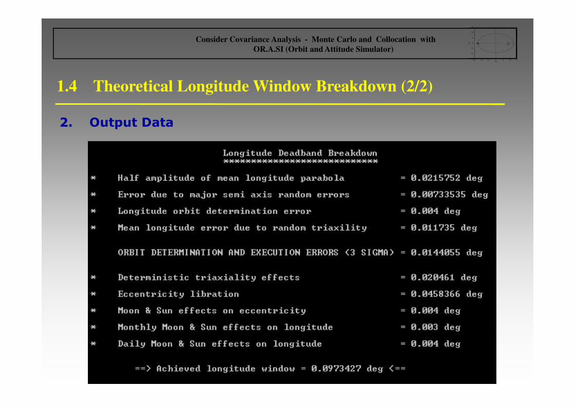
1.4 Theoretical Longitude Window Breakdown (2/2)

2. Output Data



1.5 Localization Measurements Simulator

1. Localization Measurements Simulator Characteristics

� Production of range, azimuth and elevation measurements with identically

independently distributed (iid) errors εi for whatever type of orbit and any number

of Earth stations in the relevant coverage.

� Gaussian noise distribution εi with the following characteristics:

• E(εi) = 0, zero mean value

• Var(εi) = σ2i , desired standard deviation

� Possible addition of a systematic error (constant for all campaign measurements) with

specified standard deviation and Gaussian probability distribution.

� Configuration of different measurement plan for each ground station with suitable

choice of the following parameters :

� Type of acquired measurements.

� Error standard deviation.

� Offset of the first localization session.

� Time between sessions.

� Number of sessions.



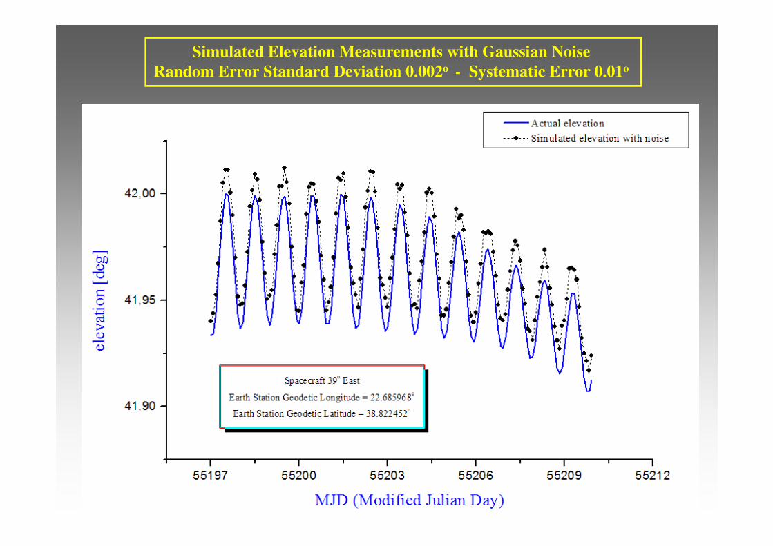
Simulated Elevation Measurements with Gaussian Noise

Random Error Standard Deviation 0.002o - Systematic Error 0.01o

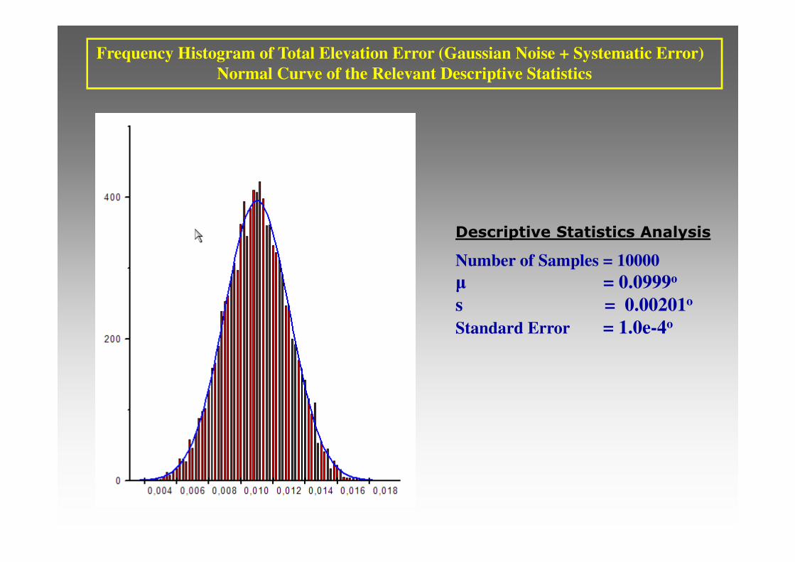
Frequency Histogram of Total Elevation Error (Gaussian Noise + Systematic Error)

Normal Curve of the Relevant Descriptive Statistics

Descriptive Statistics Analysis

Number of Samples = 10000

µ = 0.0999ο

s = 0.00201o

Standard Error = 1.0e-4o

2. Orbit Determination and

Consider Covariance Analysis



2.1 Orbit Determination with OR.A.SI (1/2)

1. Orbit Determination Module Characteristics

� Utilization of a batch weighted least-square estimator.

� Radiation pressure coefficient Cp and antenna biases for any number of the Earth

stations participating in the localization campaign, can be set as solve-for

parameters (provided that the problem formulation has good observability).

� Process of any kind of combination of tracking (azimuth-elevation) and/or range

measurements acquired from an arbitrary number of Earth stations.

� Flexibility to configure the weighted least-square estimator with suitable choice

of the following parameters :

� Combination of solve-for parameters.

� Two different measurement rejection factors. One for the first number of

iterations and another for the subsequent iterations.

� Maximum global WRMS (Weighted Root Mean Square) of residuals for

measurement rejection.

� Minimum and maximum number of iterations.

� Maximum number of divergent iterations.



2.1 Orbit Determination with OR.A.SI (2/2)

2. Output of Orbit Determination

� Quasi-Synchronous, Keplerian and Cartesian form of determined state vector.

� Standard deviation for the Keplerian form of the determined state vector.

� Standard deviation for the Cartesian form of the state vector with respect to the

satellite reference frame.

� Standard deviation of the solve-for parameters.

� Covariance matrix for the Keplerian and Cartesian state vector forms.

� Residual descriptive statistics (mean & standard deviation) for all types of

measurements taken account during the orbit determination process.

� Detection of bad observability with Singular Value Decomposition of the positive

defined matrix from the least squares normal equations and warning in case of an

ill-conditioned matrix (determinant very close to zero).



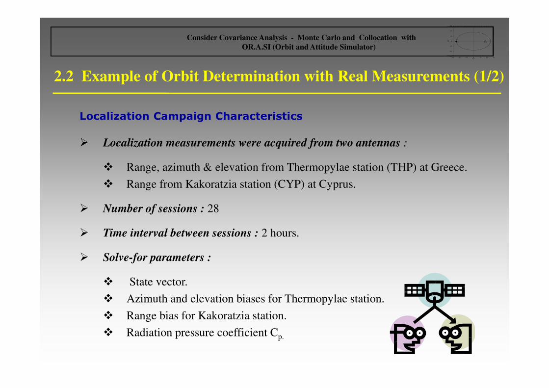
2.2 Example of Orbit Determination with Real Measurements (1/2)

Localization Campaign Characteristics

� Localization measurements were acquired from two antennas :

� Range, azimuth & elevation from Thermopylae station (THP) at Greece.

� Range from Kakoratzia station (CYP) at Cyprus.

� Number of sessions : 28

� Time interval between sessions : 2 hours.

� Solve-for parameters :

� State vector.

� Azimuth and elevation biases for Thermopylae station.

� Range bias for Kakoratzia station.

� Radiation pressure coefficient Cp.



COSMIC Results

State Vector

a = 42166.0066 Km

ex = -0.000139

ey = -0.000239

ix = 0.000185 rad

iy = -0.000832 rad

true longitude = 38.99017o

Antenna Biases

THP2 Az Bias = 0.01833o

THP2 El Bias = -0.01245o

CYP Rg Bias = -0.082 Km

Cp = 0.967

2.2 Example of Orbit Determination with Real Measurements (2/2)

OR.A.SI Results

State Vector

a = 42166.0076 Km

ex = -0.000139

ey = -0.000240

ix = 0.000187 rad

iy = -0.000832 rad


Antenna Biases

THP2 Az Bias = 0.01824o

THP2 El Bias = -0.01290o

CYP Rg Bias = -0.082 Km

Cp = 0.961



Range Residuals for Both Antennas

Why needing consider covariance analysis ?

Methods for handling bias errors in an estimation process

1. Estimated : The state vector is expanded to include dynamic and

measurement model parameters that may be in error.

PROBLEM – Too optimistic covariance matrix in the presence of systematic

no estimated errors.

2. Considered : The state vector is estimated but the uncertainty in the non-

estimated parameter is included in the estimation of the state vector and the

error covariance matrix. This assumes that the no estimated parameters are

constant and their a priori estimate and associated covariance matrix is known.

Consider covariance analysis is a technique to

assess the impact of neglecting to estimate some

parameters on the accuracy of the state estimate



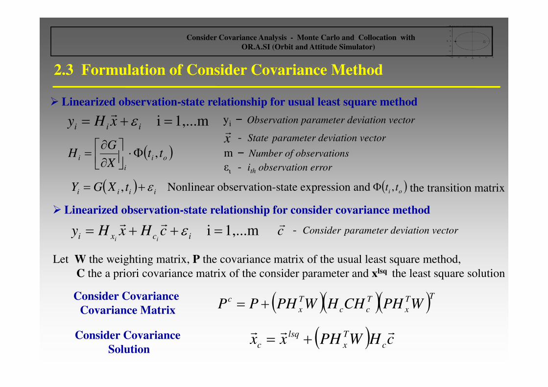
2.3 Formulation of Consider Covariance Method

1,...mi =+= iii xHy εr

� Linearized observation-state relationship for usual least square method

yi – Observation parameter deviation vector

xr

- State parameter deviation vector

m – Number of observations

ει - ith observation error

� Linearized observation-state relationship for consider covariance method

1,...mi =++= icxi cHxHyii

εrr

cr

- Consider parameter deviation vector

Let W the weighting matrix, P the covariance matrix of the usual least square method,

C the a priori covariance matrix of the consider parameter and xlsq the least square solution

( )( )( )TT

x

T

cc

T

x

cWPHCHHWPHPP +=

Consider Covariance

Covariance Matrix

Consider Covariance

Solution( ) cHWPHxx c

T

x

lsq

c

rrr+=

( )oi

i

i ttX

GH ,Φ⋅

∂∂

=

( ) iiii tXGY ε+= , Nonlinear observation-state expression and ( )oi tt ,Φ the transition matrix



Case Studies for Consider Covariance Analysis – GEO Spacecraft at 39o East (1/2)

Antenna Diameter [m] λ [deg] φ [deg] h [m] σρ [m] σΑ,Ε [deg] σ∆ρ [m] σ∆Α,∆Ε [deg]

THP 31 22.68 38.82 70 5 0.003 20 0.004

CYP 4,8 33.384 34.85 215 3 0.02 20 0.03

σR [m] σT [m] σN [m] σVr [m/s] σVt [m/s] σVn [m/s] σa [m]

Noise 75,014 292,233 692,370 0,019 0,005 0,053 11,498

Consider 95,839 994,035 767,935 0,071 0,006 0,054 43,400

0,00049

0,00140

Description (Substantial differences between estimated and consider analysis)

Case A1 One day angle and range measurements (1/2h) from THP Station ; bias parameters considered

σλ [deg]


Noise 76,744 403,478 695,919 0,0276 0,0055 0,0533 16,950

Consider 76,745 673,076 695,919 0,0480 0,0055 0,0533 16,950

0,00062

0,00096

Description (Reduction of the impact of the systematic measurement errors )

Case A2 Same as A1 but with tracking biases estimated

σλ [deg]

Determined State Vector Accuracies with respect to Satellite Reference Frame


Noise 449,689 2008,665 4536,527 0,1357 0,0326 0,3473 27,366

Consider 449,769 2464,346 4537,292 0,1709 0,0326 0,3473 27,368

0,00325

0,00378

Description (Unfavorable tracking geometry and reduced tracking performance )

Case A3 Same as A2 but with CYP Station

σλ [deg]

Case Studies for Consider Covariance Analysis – GEO Spacecraft at 39o East (2/2)


Noise 23,827 79,030 238,741 0,0048 0,0017 0,0187 1,579

Consider 28,333 781,862 241,275 0,0574 0,0019 0,0196 11,968

0,00014

0,00106

Description (Increased accuracy due to double ranging from distant stations )

Case A4 One day ranging (1/2h) from THP and CYP station ; Range biases considered

σλ [deg]


Noise 30,289 301,078 242,589 0,0224 0,0019 0,0201 14,499

Consider 30,290 616,193 242,590 0,0451 0,0019 0,0201 14,500

0,00041

0,00084

Description (Same accuracy as Case A2)

Case A5 One day ranging (1/2h) from THP and CYP station ; CYP range bias estimated

σλ [deg]


Noise 151,366 3494,062 584,922 0,2512 0,0068 0,0800 141,562

Consider 151,366 3535,434 584,922 0,2543 0,0068 0,0800 141,562

0,00482

0,00488

Description (Bud observability due to short data arc )

Case A6 12 hours ranging and tracking measurements (1/30m) from THP ; Tracking biases estimated

σλ [deg]


Noise 159,679 961,330 1782,963 0,0614 0,0121 0,0850 17,040

Consider 160,210 1285,681 1782,995 0,0871 0,0121 0,0850 20,890

0,00127

0,00173

Description (Reasonable accuracy with a very short data arc )

Case A7 6 hours ranging (1/30m) from THP and CYP stations ; Range biases considered

σλ [deg]

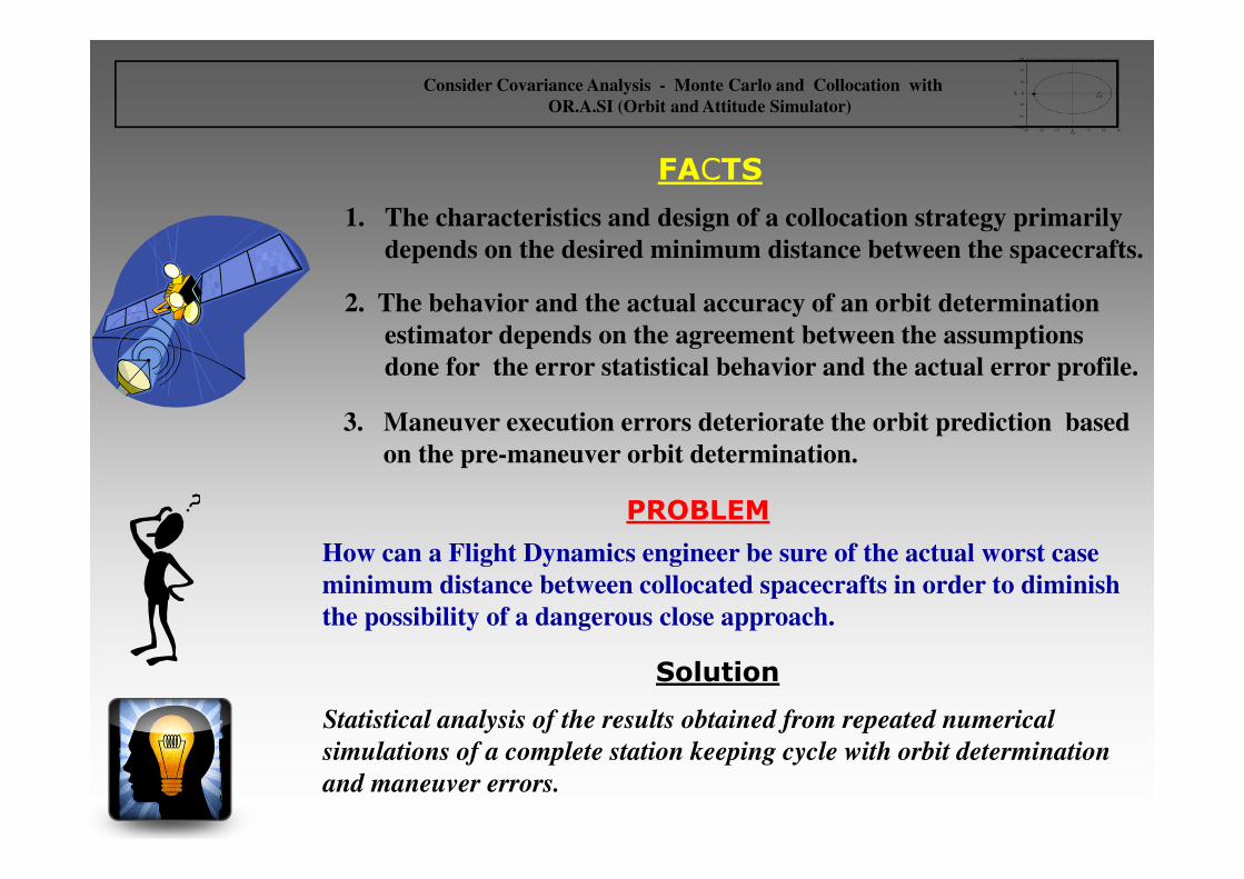
FACTS

1. The characteristics and design of a collocation strategy primarily

depends on the desired minimum distance between the spacecrafts.

2. The behavior and the actual accuracy of an orbit determination

estimator depends on the agreement between the assumptions

done for the error statistical behavior and the actual error profile.

3. Maneuver execution errors deteriorate the orbit prediction based

on the pre-maneuver orbit determination.

PROBLEM

How can a Flight Dynamics engineer be sure of the actual worst case

minimum distance between collocated spacecrafts in order to diminish

the possibility of a dangerous close approach.

Solution

Statistical analysis of the results obtained from repeated numerical

simulations of a complete station keeping cycle with orbit determination

and maneuver errors.



3. Monte Carlo

and

Orbit Determination



3.1 Monte Carlo and Orbit Determination (1/2)

1. Monte Carlo Characteristics

� Production of range, azimuth and elevation measurements having the same

characteristics and capabilities with the Localization Measurements Simulator

module.

� Capability to simulate:

� Single orbit determination.

� A full station keeping cycle comprising two pre-maneuver orbit determinations

and an inclination (South) control maneuver followed by a

longitude/eccentricity (East/West) one.

� Automatic maneuver calculation in accordance to:

� The outcome of the orbit determination based on the pre-maneuver simulated

localization measurements.

� The desired station keeping strategy, orbital location and station keeping

window dimensions.

� Reproduction of maneuver execution errors with Gaussian distribution.



3.1 Monte Carlo and Orbit Determination (2/2)

2. Monte Carlo Module Output

Data produced at the end of every iteration :

� Quasi-Synchronous (a, ex, ey, ix, iy, l) , Keplerian and Cartesian (ECF & ECI) forms

of the determined state vector.

� Mean value and covariance of the aforementioned state vector forms.

� Difference between the actual and the determined orbit in the form of quasi-

synchronous and Cartesian elements with respect to the ECF, ECI and satellite

reference frames.

� Mean value and covariance of the aforementioned differences.

Data produced at the final iteration :

� All the data listed above.

� The covariance matrices for the quasi-synchronous, Keplerian and ECI Cartesian

forms of the determined state vector.



Cross Checking Between Formal Covariances from Orbit Determination and Monte Carlo

Radial σ = 75.21 m

Standard error of σ = 0.84 m

Tangential σ = 292.83 m

Standard Error of σ = 3.29 m

Normal σ = 692.06 m

Standard Error of σ = 7.8 m

• Campaign Characteristics : 13 measurements (1/2h) - Range Noise = 5 m , Azimuth-Elevation Noise = 0.003o

• Formal Standard Deviations

from Orbit Determination :

Radial σ = 75.014 m Along Track σ = 292.233 m Cross Track σ = 692.37 m

Major Semi Axis σ = 11.5 m True Longitude = 0.000488o

Standard Deviations Acquired from Monte Carlo Descriptive Statistics (3792 samples)

• Orbit Determination Setup : Cp and antenna biases considered

Major Semi Axis σ = 11.7 m True Longitude σ = 0.000402o

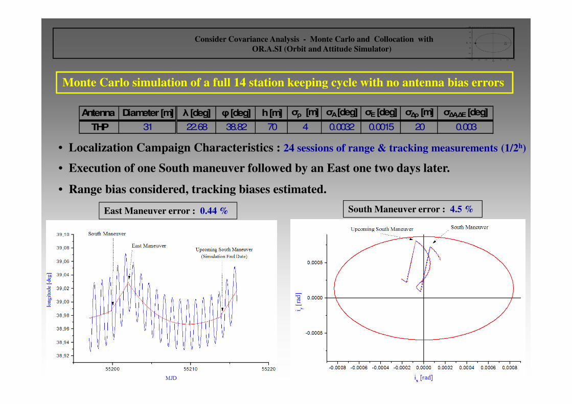
Monte Carlo simulation of a full 14 station keeping cycle with no antenna bias errors

• Localization Campaign Characteristics : 24 sessions of range & tracking measurements (1/2h)

South Maneuver error : 4.5 % East Maneuver error : 0.44 %

Antenna Diameter [m] λ [deg] φ [deg] h [m] σρ [m] σΑ [deg] σΕ [deg] σ∆ρ [m] σ∆Α,∆Ε [deg]

THP 31 22.68 38.82 70 4 0.0032 0.0015 20 0.003

• Execution of one South maneuver followed by an East one two days later.

• Range bias considered, tracking biases estimated.



Error Ellipsoid With Respect to Satellite Reference Frame

Figure 1 : Radial error with respect to tangential error

Figure 2 : 3D Scatter plot of radial, tangential and normal errors



Descriptive Statistics of Monte Carlo Results

Radial 3σ = 96 m

Standard error of 3σ = 1.2 m

Tangential 3σ = 4740 m

Standard Error of 3σ = 60 m

Normal 3σ = 909 m

Standard Error of 3σ = 11.5 m

3σ Errors for the Adapted Form of the Determined State Vector

a = 42 m ex = ey= 2·10-6 ix = iy= 1.2·10-5 rad true longitude = 0.00665o



4. Collocation Initialization



4.1 Characteristics of Collocation Initialization



� Computation of the initial state vector corresponding to one of the following modes of

collocation:

� Mode 1 : Complete longitude separation.

� Mode 2 : Longitude separation during drift cycle.

� Mode 3 : Longitude separation during eccentricity libration.

� Mode 4 : In-plane separation by eccentricity.

� Mode 5 : Inclination-eccentricity separation.

� Collocation characteristics computed in accordance to the user defined parameters:

• Epoch of collocation initialization

• Collocation mode.

• Minimum inter-satellite distance.

• Number of collocated spacecrafts.

• Maximum eccentricity.

• Eccentricity tolerance.

• Maximum allowable latitude.

• Station keeping cycle duration.

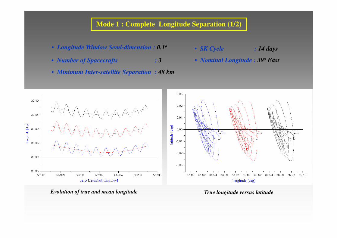
Mode 1 : Complete Longitude Separation (1/2)

• Number of Spacecrafts : 3

• SK Cycle : 14 days

• Minimum Inter-satellite Separation : 48 km

• Nominal Longitude : 39o East

• Longitude Window Semi-dimension : 0.1o

Evolution of true and mean longitude True longitude versus latitude

Mode 1 : Complete Longitude Separation (2/2)

Inter-satellite distance evolution Along track versus radial separation

Topocentric and geocentric angular separation

Mode 2 : Longitude Separation During Drift Cycle






Evolution of true and mean longitude Inter-satellite distance evolution

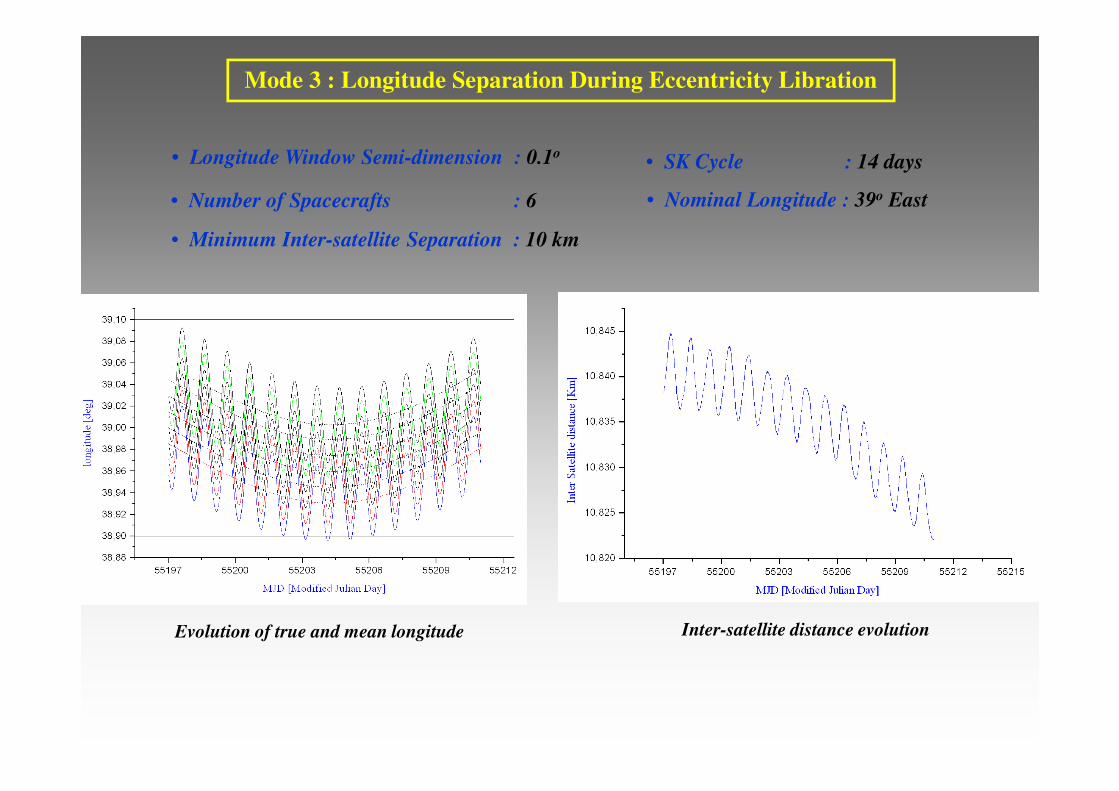
Mode 3 : Longitude Separation During Eccentricity Libration






Inter-satellite distance evolution Evolution of true and mean longitude

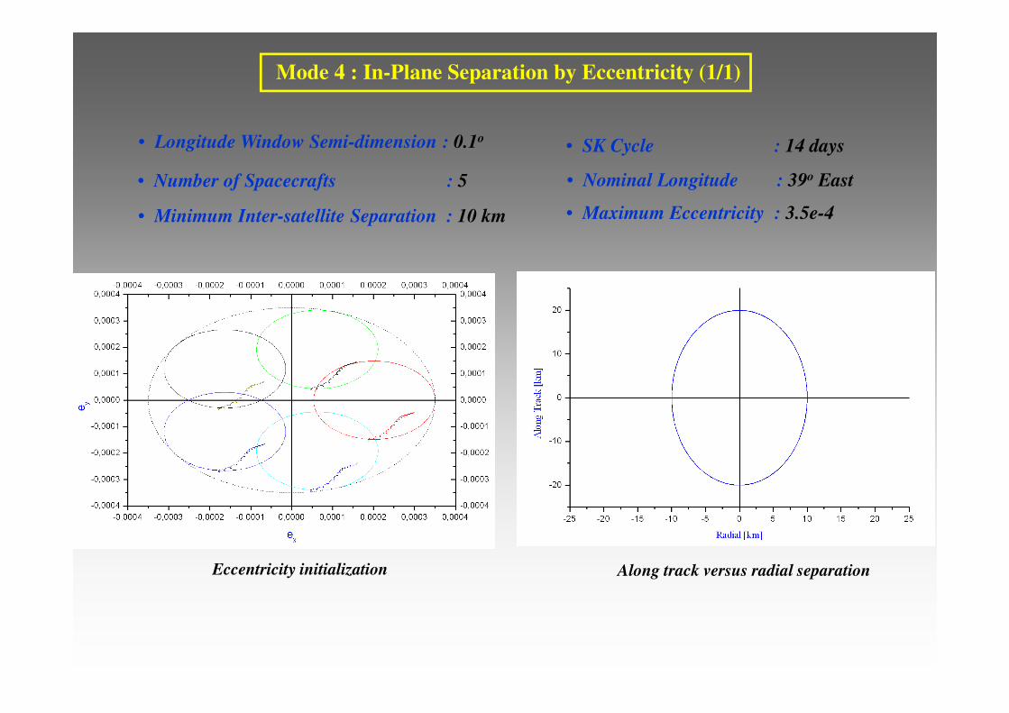
Mode 4 : In-Plane Separation by Eccentricity (1/1)






• Maximum Eccentricity : 3.5e-4

Eccentricity initialization Along track versus radial separation

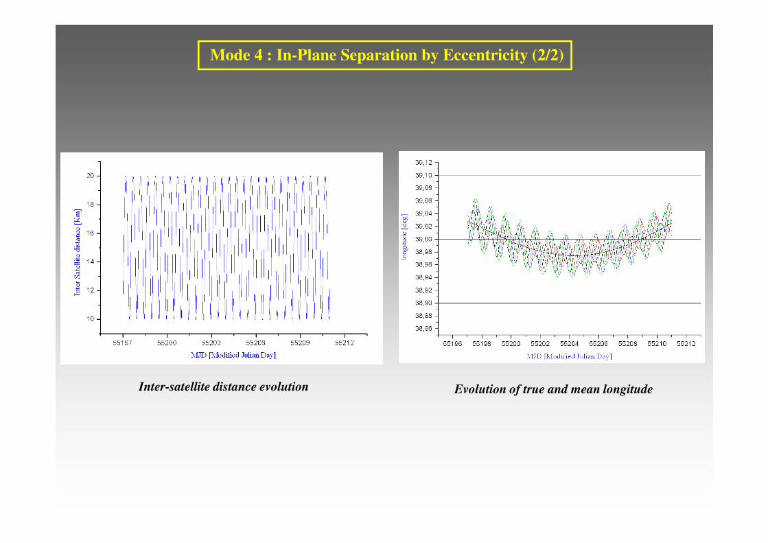
Mode 4 : In-Plane Separation by Eccentricity (2/2)

Inter-satellite distance evolution Evolution of true and mean longitude

5. Collocation Mission Analysis





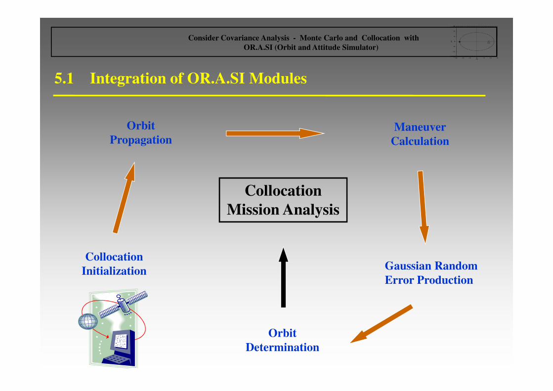
Orbit

PropagationManeuver

Calculation

Gaussian Random

Error Production

Collocation

Initialization

Orbit

Determination

Collocation

Mission Analysis

5.1 Integration of OR.A.SI Modules

5.2 Characteristics of Collocation Mission Analysis



� Initial state vector computation for each spacecraft of the collocation cluster.

� Orbit propagation.

� Production of localization measurements with Gaussian distributed errors.

� Orbit determination based on erroneous measurement production.

� Maneuver calculation based on the outcome of the orbit determination.

� Addition of maneuver execution errors.

For each pair of the collocated spacecrafts:

� Inter-satellite distance.

� Inter-satellite radial separation.

� Inter-satellite along track separation.

� Inter-satellite cross track separation.

� Inter-satellite geocentric angular separation.

� Inter-satellite angular separation with respect to a user defined Earth station.

� Eccentricity separation.

� Inclination separation.

� Angle between inter-satellite eccentricity-inclination node vectors.

� Relative velocity.

Mode 5 : Inclination-Eccentricity Separation

Desired Characteristics for Collocated Spacecrafts

• Number of spacecrafts : 3

• Minimum distance : 15 km

• Station keeping cycle : 14 days

• Nominal longitude : 39.0o East

• Longitude window semi-dimension : 0.09o

• Maximum eccentricity : 4.0e-4

• Maximum latitude : 0.05o

• Eccentricity tolerance : 5.0e-5

0

0372785.0

000355735.0

o

rrr

r

r

=×

=

=

ie

i

e

δδ

δ

δ

Separation Parameters

Initial Mean State Vectors for Epoch 01/01/2010 00:00:00

Spacecraft No.01

a = 42166.7 km

ex = 0.000203282

ey = -0.000194605

ix = 0.000750096 rad

iy = -0.000532513 rad


Spacecraft No.02

a = 42166.7 km

ex = -0.000104793

ey = -0.000372472

ix = 0.000199829 rad

iy = -0.000880893 rad


Spacecraft No.03

a = 42166.7 km

ex = -0.000104793

ey = -0.0000167378

ix = 0.000174304 rad

iy = -0.000228857 rad


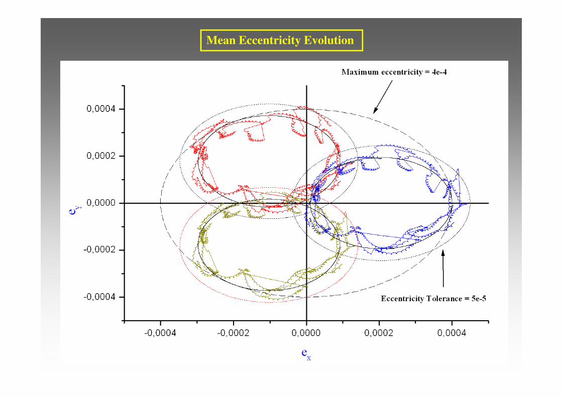
Mean Eccentricity Evolution

Mean Inclination Evolution

Inter-satellite Separation with respect to Satellite Reference Frame

Cross track versus radial separation

Along track versus radial separation

Inter-satellite Linear and Angular Separation

Inter-satellite distance evolution

Inter-satellite topocentric angular separation evolution

True Longitude and Osculating Eccentricity Evolution

True longitude evolution

Osculating eccentricity vector evolution

6. Future Plans for Further

Code Development



6.1 Future Plans for Further Code Development (1/2)



� Incorporation of maneuver velocity components as estimated parameters in orbit

determination.

� Production of more realistic simulated localization measurement sessions comprising

lots of raw measurements which are subsequently post-processed in the form of one

condensed measurement.

� Simulation of more realistic measurement and maneuver errors with the

implementation of random number generators characterized from probability

densities other than the Gaussian one.

� Detection of RF signal blockage and infrared sensor shadowing between collocated

spacecrafts.

� Adaptation of eccentricity-inclination separation collocation strategy parameters to

represent angles of inter-satellite eccentricity-inclination node vectors, different than

0o in order to decrease the possibility of mutual RF signal or infrared sensor

shadowing.

� Statistical risk assessment for collocated spacecraft collision, RF signal and infrared

sensor shadowing with the integration of the Monte Carlo and the collocation mission

analysis modules.

� Computation of inclination control maneuvers with the optimized long term control

strategy.

� Description of a realistic model for the atmosphere up to the height of 1000 Km in

order to take account the air drug perturbation for LEO calculations (Jacchia

model).

� Orbit determination based on Kalman filter sequential estimator.



6.1 Future Plans for Further Code Development (2/2)

THANK YOU FOR ATTENDING MY PRESENTATION

presentation for the 19th eurostar users conference june 2011

Documents