preﬂight spectral calibration of the orbiting...

IEEE TRANSACTIONS ON GEOSCIENCE AND REMOTE SENSING, VOL. 49, NO. 7, JULY 2011 2793

Preflight Spectral Calibration of theOrbiting Carbon Observatory

Jason O. Day, Christopher W. O’Dell, Randy Pollock, Carol J. Bruegge,David Rider, David Crisp, and Charles E. Miller

Abstract—We report on the preflight spectral calibration of thefirst Orbiting Carbon Observatory (OCO) instrument. In partic-ular, the instrument line shape (ILS) function as well as spectralposition was determined experimentally for all OCO channels. Ini-tial determination of these characteristics was conducted throughlaser-based spectroscopic measurements. The resulting spectralcalibration was validated by comparing solar spectra recordedsimultaneously by the OCO flight instrument and a collocatedhigh-resolution Fourier transform spectrometer (FTS). The spec-tral calibration was refined by optimizing parameters of the ILSas well as the dispersion relationship, which determines spectralposition, to yield the best agreement between these two measure-ments. The resulting ILS profiles showed agreement between thespectra recorded by the spectrometers and FTS to approximately0.2% rms, satisfying the preflight spectral calibration accuracyrequirement of better than 0.25% rms.

Index Terms—Carbon dioxide (CO2), instrument line shape(ILS), Orbiting Carbon Observatory (OCO), spectral calibration.

I. INTRODUCTION

THE Orbiting Carbon Observatory (OCO) was a NationalAeronautics and Space Administration (NASA) Earth

System Science Pathfinder (ESSP) mission designed to mea-sure global column CO2 concentrations twice a month with theprecision and accuracy required to detect sources and sinks onregional scales [1]–[3]. It was launched on February 24, 2009,but did not achieve orbit due to a failure of the launch vehicle.However, the details of its preflight calibration are relevant bothin their own right and as a guide for the calibration of the OCO-2 instrument, planned for launch in February 2013.

This paper describes the prelaunch spectral calibration of theOCO instrument, determined during thermal vacuum testingof the instrument at the Jet Propulsion Laboratory (JPL) inearly 2008. The radiometric calibration of OCO is describedin a companion paper [4]. The spectral calibration includes two

Manuscript received July 7, 2010; revised December 10, 2010; acceptedJanuary 16, 2011. Date of publication March 3, 2011; date of current versionJune 24, 2011.

J. O. Day was with the Department of Atmospheric Science, Colorado StateUniversity, Fort Collins, CO 80523-1371 USA. He is now with the Office ofU.S. Senator Al Franken, Washington, DC 20510 USA.

C. W. O’Dell is with the Department of Atmospheric Science, Colorado StateUniversity, Fort Collins, CO 80523-1375 USA.

R. Pollock, C. J. Bruegge, D. Rider, D. Crisp, and C. E. Miller are with theJet Propulsion Laboratory, California Institute of Technology, Pasadena, CA91109 USA.

Color versions of one or more of the figures in this paper are available onlineat http://ieeexplore.ieee.org.

Digital Object Identifier 10.1109/TGRS.2011.2107745

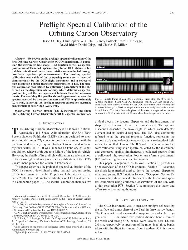
Fig. 1. Single frame of data (0.3-s exposure) from (top) the 0.76-μm O2

A-band, (middle) 1.6-μm weak CO2 band, and (bottom) 2.06-μm strong CO2

band focal plane arrays recorded by the OCO instrument while viewing themoon on February 28, 2008. Absorption features are clearly seen as dark bandsin each frame. The inset shows the phase of the moon and approximate orien-tation of the OCO spectrometer field stop when these images were acquired.

critical pieces: the spectral dispersion and the instrument lineshape (ILS) function of each detector element. The spectraldispersion describes the wavelength at which each detectorelement had its centroid response. The ILS, also commonlyreferred to as the spectral response function, represents theresponse of a single detector element to any wavelength of lightincident upon that element. The ILS and dispersion parameterswere validated using solar spectra collected by the instrumentand compared against simultaneously collected spectra froma collocated high-resolution Fourier transform spectrometer(FTS) observing the same spectral regions.

This paper is organized as follows. Section II provides abrief overview of the OCO instrument. Section III describesthe diode-laser method used to derive the spectral dispersionrelationships and ILS functions for each OCO pixel. Section IVdiscusses the validation and refinement of the laser-based spec-tral calibration using collocated observations of the sun witha high-resolution FTS. Section V summarizes this paper andoffers some concluding thoughts.

II. INSTRUMENT OVERVIEW

The OCO instrument was to measure sunlight reflected bythe surface and atmosphere of the Earth in three narrow bands.The Oxygen-A band measured absorption by molecular oxy-gen near 0.76 μm, while two carbon dioxide bands, termedthe weak and strong CO2 bands, were located near 1.6 and2.0 μm, respectively. A spectrum of the moon in all three bandstaken with the flight instrument from Pasadena, CA, is shownin Fig. 1.

0196-2892/$26.00 © 2011 IEEE

2794 IEEE TRANSACTIONS ON GEOSCIENCE AND REMOTE SENSING, VOL. 49, NO. 7, JULY 2011

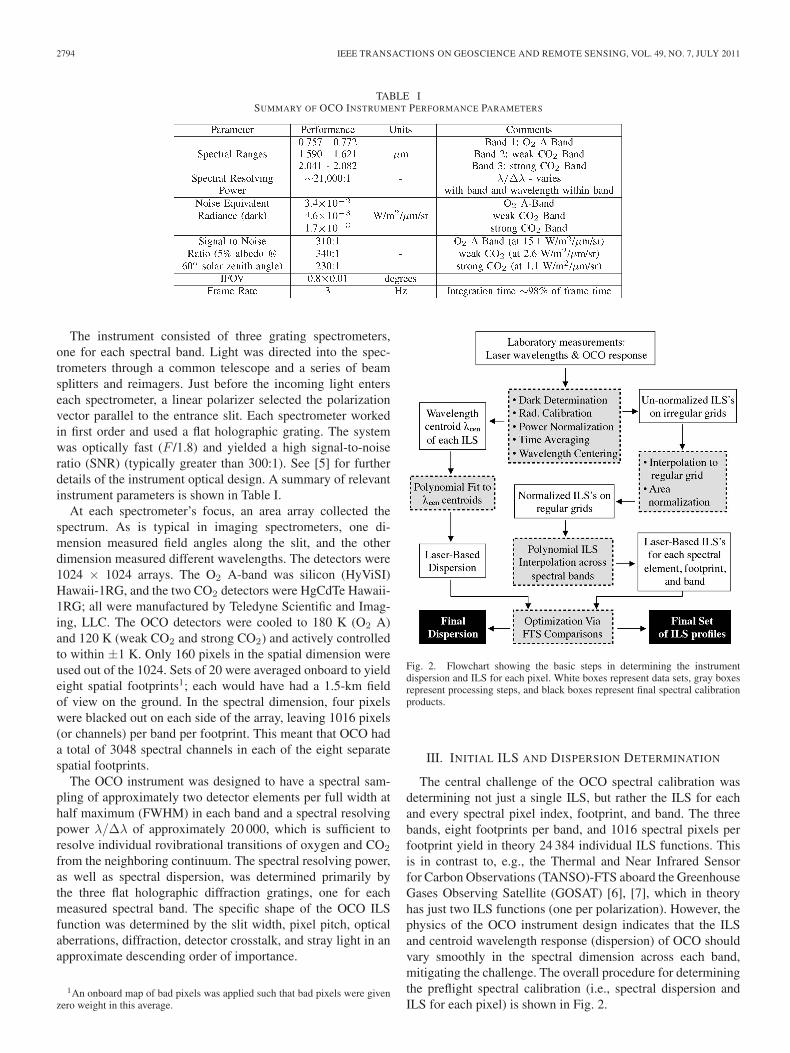
TABLE ISUMMARY OF OCO INSTRUMENT PERFORMANCE PARAMETERS

The instrument consisted of three grating spectrometers,one for each spectral band. Light was directed into the spec-trometers through a common telescope and a series of beamsplitters and reimagers. Just before the incoming light enterseach spectrometer, a linear polarizer selected the polarizationvector parallel to the entrance slit. Each spectrometer workedin first order and used a flat holographic grating. The systemwas optically fast (F /1.8) and yielded a high signal-to-noiseratio (SNR) (typically greater than 300:1). See [5] for furtherdetails of the instrument optical design. A summary of relevantinstrument parameters is shown in Table I.

At each spectrometer’s focus, an area array collected thespectrum. As is typical in imaging spectrometers, one di-mension measured field angles along the slit, and the otherdimension measured different wavelengths. The detectors were1024 × 1024 arrays. The O2 A-band was silicon (HyViSI)Hawaii-1RG, and the two CO2 detectors were HgCdTe Hawaii-1RG; all were manufactured by Teledyne Scientific and Imag-ing, LLC. The OCO detectors were cooled to 180 K (O2 A)and 120 K (weak CO2 and strong CO2) and actively controlledto within ±1 K. Only 160 pixels in the spatial dimension wereused out of the 1024. Sets of 20 were averaged onboard to yieldeight spatial footprints1; each would have had a 1.5-km fieldof view on the ground. In the spectral dimension, four pixelswere blacked out on each side of the array, leaving 1016 pixels(or channels) per band per footprint. This meant that OCO hada total of 3048 spectral channels in each of the eight separatespatial footprints.

The OCO instrument was designed to have a spectral sam-pling of approximately two detector elements per full width athalf maximum (FWHM) in each band and a spectral resolvingpower λ/Δλ of approximately 20 000, which is sufficient toresolve individual rovibrational transitions of oxygen and CO2

from the neighboring continuum. The spectral resolving power,as well as spectral dispersion, was determined primarily bythe three flat holographic diffraction gratings, one for eachmeasured spectral band. The specific shape of the OCO ILSfunction was determined by the slit width, pixel pitch, opticalaberrations, diffraction, detector crosstalk, and stray light in anapproximate descending order of importance.

1An onboard map of bad pixels was applied such that bad pixels were givenzero weight in this average.

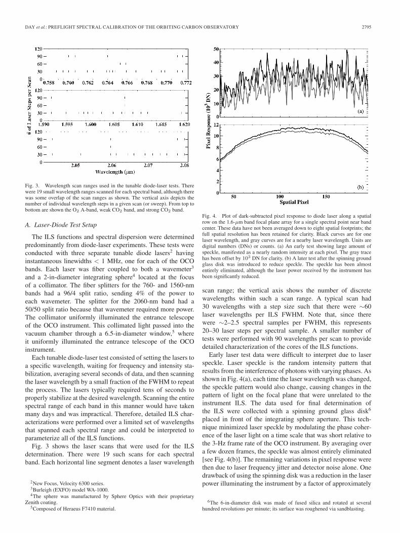
Fig. 2. Flowchart showing the basic steps in determining the instrumentdispersion and ILS for each pixel. White boxes represent data sets, gray boxesrepresent processing steps, and black boxes represent final spectral calibrationproducts.

III. INITIAL ILS AND DISPERSION DETERMINATION

The central challenge of the OCO spectral calibration wasdetermining not just a single ILS, but rather the ILS for eachand every spectral pixel index, footprint, and band. The threebands, eight footprints per band, and 1016 spectral pixels perfootprint yield in theory 24 384 individual ILS functions. Thisis in contrast to, e.g., the Thermal and Near Infrared Sensorfor Carbon Observations (TANSO)-FTS aboard the GreenhouseGases Observing Satellite (GOSAT) [6], [7], which in theoryhas just two ILS functions (one per polarization). However, thephysics of the OCO instrument design indicates that the ILSand centroid wavelength response (dispersion) of OCO shouldvary smoothly in the spectral dimension across each band,mitigating the challenge. The overall procedure for determiningthe preflight spectral calibration (i.e., spectral dispersion andILS for each pixel) is shown in Fig. 2.

DAY et al.: PREFLIGHT SPECTRAL CALIBRATION OF THE ORBITING CARBON OBSERVATORY 2795

Fig. 3. Wavelength scan ranges used in the tunable diode-laser tests. Therewere 19 small wavelength ranges scanned for each spectral band, although therewas some overlap of the scan ranges as shown. The vertical axis depicts thenumber of individual wavelength steps in a given scan (or sweep). From top tobottom are shown the O2 A-band, weak CO2 band, and strong CO2 band.

A. Laser-Diode Test Setup

The ILS functions and spectral dispersion were determinedpredominantly from diode-laser experiments. These tests wereconducted with three separate tunable diode lasers2 havinginstantaneous linewidths < 1 MHz, one for each of the OCObands. Each laser was fiber coupled to both a wavemeter3

and a 2-in-diameter integrating sphere4 located at the focusof a collimator. The fiber splitters for the 760- and 1560-nmbands had a 96/4 split ratio, sending 4% of the power toeach wavemeter. The splitter for the 2060-nm band had a50/50 split ratio because that wavemeter required more power.The collimator uniformly illuminated the entrance telescopeof the OCO instrument. This collimated light passed into thevacuum chamber through a 6.5-in-diameter window,5 whereit uniformly illuminated the entrance telescope of the OCOinstrument.

Each tunable diode-laser test consisted of setting the lasers toa specific wavelength, waiting for frequency and intensity sta-bilization, averaging several seconds of data, and then scanningthe laser wavelength by a small fraction of the FWHM to repeatthe process. The lasers typically required tens of seconds toproperly stabilize at the desired wavelength. Scanning the entirespectral range of each band in this manner would have takenmany days and was impractical. Therefore, detailed ILS char-acterizations were performed over a limited set of wavelengthsthat spanned each spectral range and could be interpreted toparameterize all of the ILS functions.

Fig. 3 shows the laser scans that were used for the ILSdetermination. There were 19 such scans for each spectralband. Each horizontal line segment denotes a laser wavelength

2New Focus, Velocity 6300 series.3Burleigh (EXFO) model WA-1000.4The sphere was manufactured by Sphere Optics with their proprietary

Zenith coating.5Composed of Heraeus F7410 material.

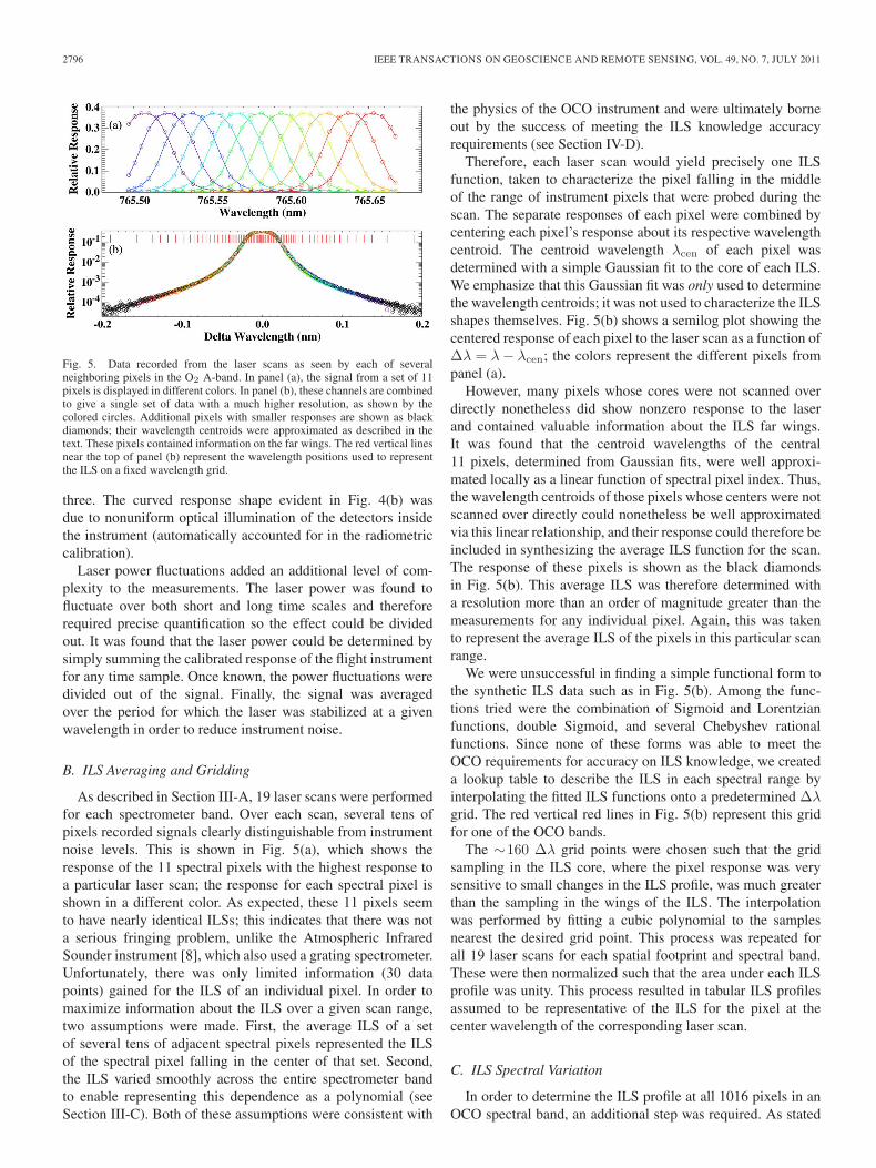
Fig. 4. Plot of dark-subtracted pixel response to diode laser along a spatialrow on the 1.6-μm band focal plane array for a single spectral point near bandcenter. These data have not been averaged down to eight spatial footprints; thefull spatial resolution has been retained for clarity. Black curves are for onelaser wavelength, and gray curves are for a nearby laser wavelength. Units aredigital numbers (DNs) or counts. (a) An early test showing large amount ofspeckle, manifested as a nearly random intensity at each pixel. The gray tracehas been offset by 103 DN for clarity. (b) A later test after the spinning groundglass disk was introduced to reduce speckle. The speckle has been almostentirely eliminated, although the laser power received by the instrument hasbeen significantly reduced.

scan range; the vertical axis shows the number of discretewavelengths within such a scan range. A typical scan had30 wavelengths with a step size such that there were ∼60laser wavelengths per ILS FWHM. Note that, since therewere ∼2–2.5 spectral samples per FWHM, this represents20–30 laser steps per spectral sample. A smaller number oftests were performed with 90 wavelengths per scan to providedetailed characterization of the cores of the ILS functions.

Early laser test data were difficult to interpret due to laserspeckle. Laser speckle is the random intensity pattern thatresults from the interference of photons with varying phases. Asshown in Fig. 4(a), each time the laser wavelength was changed,the speckle pattern would also change, causing changes in thepattern of light on the focal plane that were unrelated to theinstrument ILS. The data used for final determination ofthe ILS were collected with a spinning ground glass disk6

placed in front of the integrating sphere aperture. This tech-nique minimized laser speckle by modulating the phase coher-ence of the laser light on a time scale that was short relative tothe 3-Hz frame rate of the OCO instrument. By averaging overa few dozen frames, the speckle was almost entirely eliminated[see Fig. 4(b)]. The remaining variations in pixel response werethen due to laser frequency jitter and detector noise alone. Onedrawback of using the spinning disk was a reduction in the laserpower illuminating the instrument by a factor of approximately

6The 6-in-diameter disk was made of fused silica and rotated at severalhundred revolutions per minute; its surface was roughened via sandblasting.


Fig. 5. Data recorded from the laser scans as seen by each of severalneighboring pixels in the O2 A-band. In panel (a), the signal from a set of 11pixels is displayed in different colors. In panel (b), these channels are combinedto give a single set of data with a much higher resolution, as shown by thecolored circles. Additional pixels with smaller responses are shown as blackdiamonds; their wavelength centroids were approximated as described in thetext. These pixels contained information on the far wings. The red vertical linesnear the top of panel (b) represent the wavelength positions used to representthe ILS on a fixed wavelength grid.

three. The curved response shape evident in Fig. 4(b) wasdue to nonuniform optical illumination of the detectors insidethe instrument (automatically accounted for in the radiometriccalibration).

Laser power fluctuations added an additional level of com-plexity to the measurements. The laser power was found tofluctuate over both short and long time scales and thereforerequired precise quantification so the effect could be dividedout. It was found that the laser power could be determined bysimply summing the calibrated response of the flight instrumentfor any time sample. Once known, the power fluctuations weredivided out of the signal. Finally, the signal was averagedover the period for which the laser was stabilized at a givenwavelength in order to reduce instrument noise.

B. ILS Averaging and Gridding

As described in Section III-A, 19 laser scans were performedfor each spectrometer band. Over each scan, several tens ofpixels recorded signals clearly distinguishable from instrumentnoise levels. This is shown in Fig. 5(a), which shows theresponse of the 11 spectral pixels with the highest response toa particular laser scan; the response for each spectral pixel isshown in a different color. As expected, these 11 pixels seemto have nearly identical ILSs; this indicates that there was nota serious fringing problem, unlike the Atmospheric InfraredSounder instrument [8], which also used a grating spectrometer.Unfortunately, there was only limited information (30 datapoints) gained for the ILS of an individual pixel. In order tomaximize information about the ILS over a given scan range,two assumptions were made. First, the average ILS of a setof several tens of adjacent spectral pixels represented the ILSof the spectral pixel falling in the center of that set. Second,the ILS varied smoothly across the entire spectrometer bandto enable representing this dependence as a polynomial (seeSection III-C). Both of these assumptions were consistent with

the physics of the OCO instrument and were ultimately borneout by the success of meeting the ILS knowledge accuracyrequirements (see Section IV-D).

Therefore, each laser scan would yield precisely one ILSfunction, taken to characterize the pixel falling in the middleof the range of instrument pixels that were probed during thescan. The separate responses of each pixel were combined bycentering each pixel’s response about its respective wavelengthcentroid. The centroid wavelength λcen of each pixel wasdetermined with a simple Gaussian fit to the core of each ILS.We emphasize that this Gaussian fit was only used to determinethe wavelength centroids; it was not used to characterize the ILSshapes themselves. Fig. 5(b) shows a semilog plot showing thecentered response of each pixel to the laser scan as a function ofΔλ = λ− λcen; the colors represent the different pixels frompanel (a).

However, many pixels whose cores were not scanned overdirectly nonetheless did show nonzero response to the laserand contained valuable information about the ILS far wings.It was found that the centroid wavelengths of the central11 pixels, determined from Gaussian fits, were well approxi-mated locally as a linear function of spectral pixel index. Thus,the wavelength centroids of those pixels whose centers were notscanned over directly could nonetheless be well approximatedvia this linear relationship, and their response could therefore beincluded in synthesizing the average ILS function for the scan.The response of these pixels is shown as the black diamondsin Fig. 5(b). This average ILS was therefore determined witha resolution more than an order of magnitude greater than themeasurements for any individual pixel. Again, this was takento represent the average ILS of the pixels in this particular scanrange.

We were unsuccessful in finding a simple functional form tothe synthetic ILS data such as in Fig. 5(b). Among the func-tions tried were the combination of Sigmoid and Lorentzianfunctions, double Sigmoid, and several Chebyshev rationalfunctions. Since none of these forms was able to meet theOCO requirements for accuracy on ILS knowledge, we createda lookup table to describe the ILS in each spectral range byinterpolating the fitted ILS functions onto a predetermined Δλgrid. The red vertical red lines in Fig. 5(b) represent this gridfor one of the OCO bands.

The ∼160 Δλ grid points were chosen such that the gridsampling in the ILS core, where the pixel response was verysensitive to small changes in the ILS profile, was much greaterthan the sampling in the wings of the ILS. The interpolationwas performed by fitting a cubic polynomial to the samplesnearest the desired grid point. This process was repeated forall 19 laser scans for each spatial footprint and spectral band.These were then normalized such that the area under each ILSprofile was unity. This process resulted in tabular ILS profilesassumed to be representative of the ILS for the pixel at thecenter wavelength of the corresponding laser scan.

C. ILS Spectral Variation

In order to determine the ILS profile at all 1016 pixels in anOCO spectral band, an additional step was required. As stated


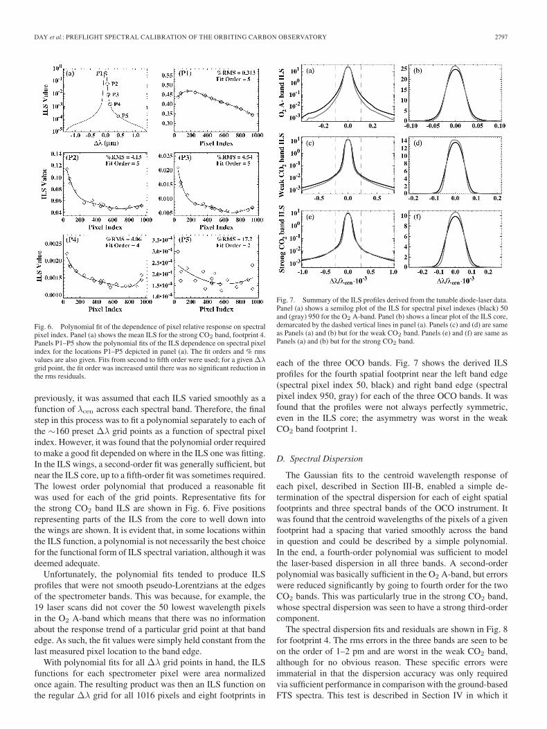
Fig. 6. Polynomial fit of the dependence of pixel relative response on spectralpixel index. Panel (a) shows the mean ILS for the strong CO2 band, footprint 4.Panels P1–P5 show the polynomial fits of the ILS dependence on spectral pixelindex for the locations P1–P5 depicted in panel (a). The fit orders and % rmsvalues are also given. Fits from second to fifth order were used; for a given Δλgrid point, the fit order was increased until there was no significant reduction inthe rms residuals.

previously, it was assumed that each ILS varied smoothly as afunction of λcen across each spectral band. Therefore, the finalstep in this process was to fit a polynomial separately to each ofthe ∼160 preset Δλ grid points as a function of spectral pixelindex. However, it was found that the polynomial order requiredto make a good fit depended on where in the ILS one was fitting.In the ILS wings, a second-order fit was generally sufficient, butnear the ILS core, up to a fifth-order fit was sometimes required.The lowest order polynomial that produced a reasonable fitwas used for each of the grid points. Representative fits forthe strong CO2 band ILS are shown in Fig. 6. Five positionsrepresenting parts of the ILS from the core to well down intothe wings are shown. It is evident that, in some locations withinthe ILS function, a polynomial is not necessarily the best choicefor the functional form of ILS spectral variation, although it wasdeemed adequate.

Unfortunately, the polynomial fits tended to produce ILSprofiles that were not smooth pseudo-Lorentzians at the edgesof the spectrometer bands. This was because, for example, the19 laser scans did not cover the 50 lowest wavelength pixelsin the O2 A-band which means that there was no informationabout the response trend of a particular grid point at that bandedge. As such, the fit values were simply held constant from thelast measured pixel location to the band edge.

With polynomial fits for all Δλ grid points in hand, the ILSfunctions for each spectrometer pixel were area normalizedonce again. The resulting product was then an ILS function onthe regular Δλ grid for all 1016 pixels and eight footprints in

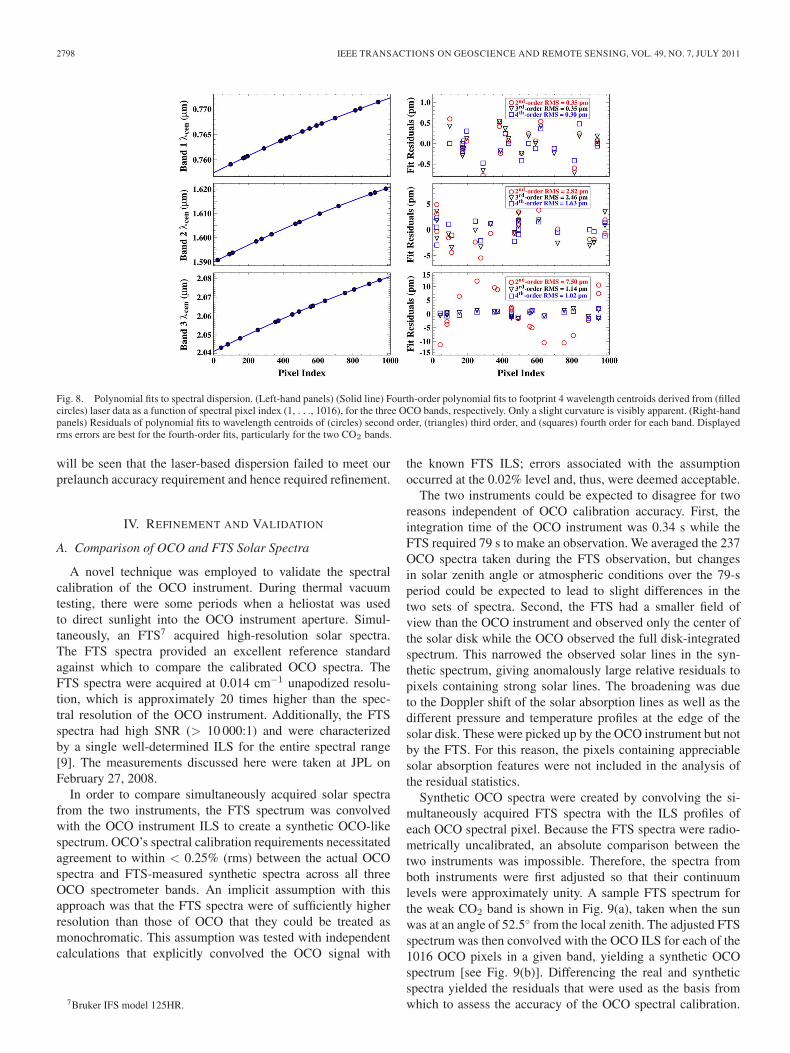
Fig. 7. Summary of the ILS profiles derived from the tunable diode-laser data.Panel (a) shows a semilog plot of the ILS for spectral pixel indexes (black) 50and (gray) 950 for the O2 A-band. Panel (b) shows a linear plot of the ILS core,demarcated by the dashed vertical lines in panel (a). Panels (c) and (d) are sameas Panels (a) and (b) but for the weak CO2 band. Panels (e) and (f) are same asPanels (a) and (b) but for the strong CO2 band.

each of the three OCO bands. Fig. 7 shows the derived ILSprofiles for the fourth spatial footprint near the left band edge(spectral pixel index 50, black) and right band edge (spectralpixel index 950, gray) for each of the three OCO bands. It wasfound that the profiles were not always perfectly symmetric,even in the ILS core; the asymmetry was worst in the weakCO2 band footprint 1.

D. Spectral Dispersion

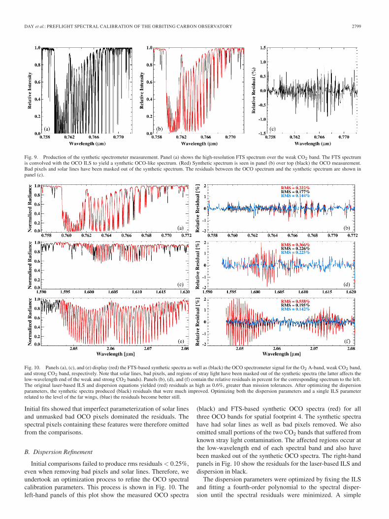
The Gaussian fits to the centroid wavelength response ofeach pixel, described in Section III-B, enabled a simple de-termination of the spectral dispersion for each of eight spatialfootprints and three spectral bands of the OCO instrument. Itwas found that the centroid wavelengths of the pixels of a givenfootprint had a spacing that varied smoothly across the bandin question and could be described by a simple polynomial.In the end, a fourth-order polynomial was sufficient to modelthe laser-based dispersion in all three bands. A second-orderpolynomial was basically sufficient in the O2 A-band, but errorswere reduced significantly by going to fourth order for the twoCO2 bands. This was particularly true in the strong CO2 band,whose spectral dispersion was seen to have a strong third-ordercomponent.

The spectral dispersion fits and residuals are shown in Fig. 8for footprint 4. The rms errors in the three bands are seen to beon the order of 1–2 pm and are worst in the weak CO2 band,although for no obvious reason. These specific errors wereimmaterial in that the dispersion accuracy was only requiredvia sufficient performance in comparison with the ground-basedFTS spectra. This test is described in Section IV in which it


Fig. 8. Polynomial fits to spectral dispersion. (Left-hand panels) (Solid line) Fourth-order polynomial fits to footprint 4 wavelength centroids derived from (filledcircles) laser data as a function of spectral pixel index (1, . . ., 1016), for the three OCO bands, respectively. Only a slight curvature is visibly apparent. (Right-handpanels) Residuals of polynomial fits to wavelength centroids of (circles) second order, (triangles) third order, and (squares) fourth order for each band. Displayedrms errors are best for the fourth-order fits, particularly for the two CO2 bands.

will be seen that the laser-based dispersion failed to meet ourprelaunch accuracy requirement and hence required refinement.

IV. REFINEMENT AND VALIDATION

A. Comparison of OCO and FTS Solar Spectra

A novel technique was employed to validate the spectralcalibration of the OCO instrument. During thermal vacuumtesting, there were some periods when a heliostat was usedto direct sunlight into the OCO instrument aperture. Simul-taneously, an FTS7 acquired high-resolution solar spectra.The FTS spectra provided an excellent reference standardagainst which to compare the calibrated OCO spectra. TheFTS spectra were acquired at 0.014 cm−1 unapodized resolu-tion, which is approximately 20 times higher than the spec-tral resolution of the OCO instrument. Additionally, the FTSspectra had high SNR (> 10 000:1) and were characterizedby a single well-determined ILS for the entire spectral range[9]. The measurements discussed here were taken at JPL onFebruary 27, 2008.

In order to compare simultaneously acquired solar spectrafrom the two instruments, the FTS spectrum was convolvedwith the OCO instrument ILS to create a synthetic OCO-likespectrum. OCO’s spectral calibration requirements necessitatedagreement to within < 0.25% (rms) between the actual OCOspectra and FTS-measured synthetic spectra across all threeOCO spectrometer bands. An implicit assumption with thisapproach was that the FTS spectra were of sufficiently higherresolution than those of OCO that they could be treated asmonochromatic. This assumption was tested with independentcalculations that explicitly convolved the OCO signal with

7Bruker IFS model 125HR.

the known FTS ILS; errors associated with the assumptionoccurred at the 0.02% level and, thus, were deemed acceptable.

The two instruments could be expected to disagree for tworeasons independent of OCO calibration accuracy. First, theintegration time of the OCO instrument was 0.34 s while theFTS required 79 s to make an observation. We averaged the 237OCO spectra taken during the FTS observation, but changesin solar zenith angle or atmospheric conditions over the 79-speriod could be expected to lead to slight differences in thetwo sets of spectra. Second, the FTS had a smaller field ofview than the OCO instrument and observed only the center ofthe solar disk while the OCO observed the full disk-integratedspectrum. This narrowed the observed solar lines in the syn-thetic spectrum, giving anomalously large relative residuals topixels containing strong solar lines. The broadening was dueto the Doppler shift of the solar absorption lines as well as thedifferent pressure and temperature profiles at the edge of thesolar disk. These were picked up by the OCO instrument but notby the FTS. For this reason, the pixels containing appreciablesolar absorption features were not included in the analysis ofthe residual statistics.

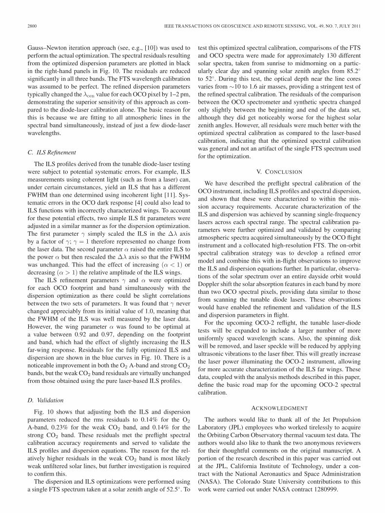
Synthetic OCO spectra were created by convolving the si-multaneously acquired FTS spectra with the ILS profiles ofeach OCO spectral pixel. Because the FTS spectra were radio-metrically uncalibrated, an absolute comparison between thetwo instruments was impossible. Therefore, the spectra fromboth instruments were first adjusted so that their continuumlevels were approximately unity. A sample FTS spectrum forthe weak CO2 band is shown in Fig. 9(a), taken when the sunwas at an angle of 52.5◦ from the local zenith. The adjusted FTSspectrum was then convolved with the OCO ILS for each of the1016 OCO pixels in a given band, yielding a synthetic OCOspectrum [see Fig. 9(b)]. Differencing the real and syntheticspectra yielded the residuals that were used as the basis fromwhich to assess the accuracy of the OCO spectral calibration.


Fig. 9. Production of the synthetic spectrometer measurement. Panel (a) shows the high-resolution FTS spectrum over the weak CO2 band. The FTS spectrumis convolved with the OCO ILS to yield a synthetic OCO-like spectrum. (Red) Synthetic spectrum is seen in panel (b) over top (black) the OCO measurement.Bad pixels and solar lines have been masked out of the synthetic spectrum. The residuals between the OCO spectrum and the synthetic spectrum are shown inpanel (c).

Fig. 10. Panels (a), (c), and (e) display (red) the FTS-based synthetic spectra as well as (black) the OCO spectrometer signal for the O2 A-band, weak CO2 band,and strong CO2 band, respectively. Note that solar lines, bad pixels, and regions of stray light have been masked out of the synthetic spectra (the latter affects thelow-wavelength end of the weak and strong CO2 bands). Panels (b), (d), and (f) contain the relative residuals in percent for the corresponding spectrum to the left.The original laser-based ILS and dispersion equations yielded (red) residuals as high as 0.6%, greater than mission tolerances. After optimizing the dispersionparameters, the synthetic spectra produced (black) residuals that were much improved. Optimizing both the dispersion parameters and a single ILS parameterrelated to the level of the far wings, (blue) the residuals become better still.

Initial fits showed that imperfect parameterization of solar linesand unmasked bad OCO pixels dominated the residuals. Thespectral pixels containing these features were therefore omittedfrom the comparisons.

B. Dispersion Refinement

Initial comparisons failed to produce rms residuals < 0.25%,even when removing bad pixels and solar lines. Therefore, weundertook an optimization process to refine the OCO spectralcalibration parameters. This process is shown in Fig. 10. Theleft-hand panels of this plot show the measured OCO spectra

(black) and FTS-based synthetic OCO spectra (red) for allthree OCO bands for spatial footprint 4. The synthetic spectrahave had solar lines as well as bad pixels removed. We alsoomitted small portions of the two CO2 bands that suffered fromknown stray light contamination. The affected regions occur atthe low-wavelength end of each spectral band and also havebeen masked out of the synthetic OCO spectra. The right-handpanels in Fig. 10 show the residuals for the laser-based ILS anddispersion in black.

The dispersion parameters were optimized by fixing the ILSand fitting a fourth-order polynomial to the spectral disper-sion until the spectral residuals were minimized. A simple


Gauss–Newton iteration approach (see, e.g., [10]) was used toperform the actual optimization. The spectral residuals resultingfrom the optimized dispersion parameters are plotted in blackin the right-hand panels in Fig. 10. The residuals are reducedsignificantly in all three bands. The FTS wavelength calibrationwas assumed to be perfect. The refined dispersion parameterstypically changed the λcen value for each OCO pixel by 1–2 pm,demonstrating the superior sensitivity of this approach as com-pared to the diode-laser calibration alone. The basic reason forthis is because we are fitting to all atmospheric lines in thespectral band simultaneously, instead of just a few diode-laserwavelengths.

C. ILS Refinement

The ILS profiles derived from the tunable diode-laser testingwere subject to potential systematic errors. For example, ILSmeasurements using coherent light (such as from a laser) can,under certain circumstances, yield an ILS that has a differentFWHM than one determined using incoherent light [11]. Sys-tematic errors in the OCO dark response [4] could also lead toILS functions with incorrectly characterized wings. To accountfor these potential effects, two simple ILS fit parameters wereadjusted in a similar manner as for the dispersion optimization.The first parameter γ simply scaled the ILS in the Δλ axisby a factor of γ; γ = 1 therefore represented no change fromthe laser data. The second parameter α raised the entire ILS tothe power α but then rescaled the Δλ axis so that the FWHMwas unchanged. This had the effect of increasing (α < 1) ordecreasing (α > 1) the relative amplitude of the ILS wings.

The ILS refinement parameters γ and α were optimizedfor each OCO footprint and band simultaneously with thedispersion optimization as there could be slight correlationsbetween the two sets of parameters. It was found that γ neverchanged appreciably from its initial value of 1.0, meaning thatthe FWHM of the ILS was well measured by the laser data.However, the wing parameter α was found to be optimal ata value between 0.92 and 0.97, depending on the footprintand band, which had the effect of slightly increasing the ILSfar-wing response. Residuals for the fully optimized ILS anddispersion are shown in the blue curves in Fig. 10. There is anoticeable improvement in both the O2 A-band and strong CO2

bands, but the weak CO2 band residuals are virtually unchangedfrom those obtained using the pure laser-based ILS profiles.

D. Validation

Fig. 10 shows that adjusting both the ILS and dispersionparameters reduced the rms residuals to 0.14% for the O2

A-band, 0.23% for the weak CO2 band, and 0.14% for thestrong CO2 band. These residuals met the preflight spectralcalibration accuracy requirements and served to validate theILS profiles and dispersion equations. The reason for the rel-atively higher residuals in the weak CO2 band is most likelyweak unfiltered solar lines, but further investigation is requiredto confirm this.

The dispersion and ILS optimizations were performed usinga single FTS spectrum taken at a solar zenith angle of 52.5◦. To

test this optimized spectral calibration, comparisons of the FTSand OCO spectra were made for approximately 130 differentsolar spectra, taken from sunrise to midmorning on a partic-ularly clear day and spanning solar zenith angles from 85.2◦

to 52◦. During this test, the optical depth near the line coresvaries from ∼10 to 1.6 air masses, providing a stringent test ofthe refined spectral calibration. The residuals of the comparisonbetween the OCO spectrometer and synthetic spectra changedonly slightly between the beginning and end of the data set,although they did get noticeably worse for the highest solarzenith angles. However, all residuals were much better with theoptimized spectral calibration as compared to the laser-basedcalibration, indicating that the optimized spectral calibrationwas general and not an artifact of the single FTS spectrum usedfor the optimization.

V. CONCLUSION

We have described the preflight spectral calibration of theOCO instrument, including ILS profiles and spectral dispersion,and shown that these were characterized to within the mis-sion accuracy requirements. Accurate characterization of theILS and dispersion was achieved by scanning single-frequencylasers across each spectral range. The spectral calibration pa-rameters were further optimized and validated by comparingatmospheric spectra acquired simultaneously by the OCO flightinstrument and a collocated high-resolution FTS. The on-orbitspectral calibration strategy was to develop a refined errormodel and combine this with in-flight observations to improvethe ILS and dispersion equations further. In particular, observa-tions of the solar spectrum over an entire dayside orbit wouldDoppler shift the solar absorption features in each band by morethan two OCO spectral pixels, providing data similar to thosefrom scanning the tunable diode lasers. These observationswould have enabled the refinement and validation of the ILSand dispersion parameters in flight.

For the upcoming OCO-2 reflight, the tunable laser-diodetests will be expanded to include a larger number of moreuniformly spaced wavelength scans. Also, the spinning diskwill be removed, and laser speckle will be reduced by applyingultrasonic vibrations to the laser fiber. This will greatly increasethe laser power illuminating the OCO-2 instrument, allowingfor more accurate characterization of the ILS far wings. Thesedata, coupled with the analysis methods described in this paper,define the basic road map for the upcoming OCO-2 spectralcalibration.

ACKNOWLEDGMENT

The authors would like to thank all of the Jet PropulsionLaboratory (JPL) employees who worked tirelessly to acquirethe Orbiting Carbon Observatory thermal vacuum test data. Theauthors would also like to thank the two anonymous reviewersfor their thoughtful comments on the original manuscript. Aportion of the research described in this paper was carried outat the JPL, California Institute of Technology, under a con-tract with the National Aeronautics and Space Administration(NASA). The Colorado State University contributions to thiswork were carried out under NASA contract 1280999.


REFERENCES

[1] D. Crisp, R. M. Atlas, F.-M. Breon, L. R. Brown, J. P. Burrows, P. Ciais,B. J. Connor, S. C. Doney, I. Y. Fung, D. J. Jacob, C. E. Miller, D. O’Brien,S. Pawson, J. T. Randerson, P. Rayner, R. J. Salawitch, S. P. Sander,B. Sen, G. L. Stephens, P. P. Tans, G. C. Toon, P. O. Wennberg,S. C. Wofsy, Y. L. Yung, Z. Kuang, B. Chudasama, G. Sprague, B. Weiss,R. Pollock, D. Kenyon, and S. Schroll, “The Orbiting Carbon Observatory(OCO) mission,” Adv. Space Res., vol. 34, no. 4, pp. 700–709, 2004.

[2] D. Crisp and C. Johnson, “The Orbiting Carbon Observatory mission,”Acta Astronaut., vol. 56, no. 1/2, pp. 193–197, Jan. 2005.

[3] C. E. Miller, D. Crisp, P. L. DeCola, S. C. Olsen, J. T. Randerson,A. M. Michalak, A. Alkhaled, P. Rayner, D. J. Jacob, P. Suntharalingam,D. B. A. Jones, A. S. Denning, M. E. Nicholls, S. C. Doney, S. Pawson,H. Boesch, B. J. Connor, I. Y. Fung, D. O’Brien, R. J. Salawitch,S. P. Sander, B. Sen, P. Tans, G. C. Toon, P. O. Wennberg, S. C. Wofsy,Y. L. Yung, and R. M. Law, “Precision requirements for space-basedXCO2

data,” J. Geophys. Res., vol. 112, p. D10 314, May 2007.[4] C. W. O’Dell, J. O. Day, C. Bruegge, R. Castano, D. Crisp, C. E. Miller,

D. M. O’Brien, R. Pollock, and I. Tkatcheva, “Preflight radiometric cali-bration of the Orbiting Carbon Observatory,” IEEE Trans. Geosci. RemoteSens., 2011, to be published.

[5] R. Haring, R. Pollock, B. Sutin, and D. Crisp, “Current development statusof the Orbiting Carbon Observatory instrument optical design,” in Proc.SPIE, M. Strojnik, Ed., 2005, vol. 5883, no. 1, p. 588 30C.

[6] T. Hamazaki, Y. Kaneko, A. Kuze, and H. Suto, “Greenhouse gases obser-vation from space with TANSO-FTS on GOSAT,” presented at the FourierTransform Spectroscopy/Hyperspectral Imaging Sounding Environment,Santa Fe, NM, 2007, Paper FWB1.

[7] H. Suto, T. Kawashima, J. Yoshida, J. Ishida, A. Kuze, M. Nakajima, andT. Hamazaki, “The pre-launch performance test and calibration resultsof Thermal And Near-infrared Sensor for carbon Observation (TANSO)on GOSAT,” in Proc. SPIE, R. Meynart, S. P. Neeck, H. Shimoda, andS. Habib, Eds., 2008, vol. 7106, no. 1, p. 710 60L.

[8] L. L. Strow, S. E. Hannon, M. Weiler, K. Overoye, S. L. Gaiser, andH. H. Aumann, “Prelaunch spectral calibration of the atmospheric infraredsounder (AIRS),” IEEE Trans. Geosci. Remote Sens., vol. 41, no. 2,pp. 274–286, Feb. 2003.

[9] R. A. Washenfelder, G. C. Toon, J.-F. Blavier, Z. Yang, N. T. Allen,P. O. Wennberg, S. A. Vay, D. M. Matross, and B. C. Daube, “Carbondioxide column abundances at the Wisconsin Tall Tower site,” J. Geophys.Res., vol. 111, p. D22 305, 2006.

[10] C. D. Rodgers, Inverse Methods for Atmospheric Sounding: Theory andPractice. Singapore: World Scientific, 2000.

[11] P. Mouroulis and R. O. Green, “Spectral response evaluation andcomputation for pushbroom imaging spectrometers,” in Proc. SPIE,P. Z. Mouroulis, W. J. Smith, and R. B. Johnson, Eds., 2007, vol. 6667,no. 1, p. 666 70G.

Jason O. Day received the Ph.D. degree inatomic physics from the University of Wisconsin,Madison.

From 2008 to 2009, he was a Postdoctoral Fellowwith the Orbiting Carbon Observatory team. He iscurrently an American Geophysical Union Congres-sional Science Fellow with the Office of U.S. SenatorAl Franken.

Christopher W. O’Dell received the Ph.D. degree inphysics from the University of Wisconsin, Madison,in 2001, where he studied the cosmic microwavebackground radiation.

After postdoctoral positions in both astronomyand microwave remote sensing, he joined the re-search staff with Colorado State University, FortCollins, in 2007, where he is currently a Member ofthe Cooperative Institute on Research in the Atmo-sphere. His research concerns the remote sensing ofclimatically important atmospheric variables such as

water vapor and carbon dioxide.

Randy Pollock received the B.S. degree in engineer-ing and applied science from the California Instituteof Technology, Pasadena, in 1991.

He is currently an Instrument Architect for theOrbiting Carbon Observatory with the Jet PropulsionLaboratory, California Institute of Technology.

Carol J. (Kastner) Bruegge received the Ph.D.degree in optical sciences from the University ofArizona, Tucson, in 1985.

From 1988 to 2003, she was a Member ofthe Earth Observing System Multi-angle ImagingSpectroRadiometer team. She was a Principal In-vestigator of the LED Spectrometer (LSpec) auto-matic vicarious calibration facility and also the FirstInternational Satellite Land Surface ClimatologyProgram Field Experiment, a ground-truth hydrologyexperiment conducted from 1987 to 1992. She is

currently with the Jet Propulsion Laboratory, California Institute of Technology,Pasadena, where she is a Member of the Orbiting Carbon Observatory scienceteam.

David Rider received the Ph.D. degree in physi-cal chemistry from Michigan State University, EastLansing.

He came to the Jet Propulsion Laboratory (JPL),California Institute of Technology, Pasadena, in 1983after completing his Ph.D. studies at Michigan Stateand then postdoctoral research at Stanford Univer-sity. At JPL he worked on the development of awide variety of atmospheric remote sensing instru-mentation for both planetary and Earth missions.More recently he was Instrument Scientist for the

Tropospheric Emission Spectrometer (TES) on NASA’s Aura Earth ObservingSpacecraft. He is currently the Instrument Scientist for the Orbiting CarbonObservatory.

David Crisp is an Atmospheric Physicist and aSenior Research Scientist at the Jet Propulsion Labo-ratory, California Institute of Technology, Pasadena.He was the Principal Investigator of the Earth SystemScience Pathfinder (ESSP) Orbiting Carbon Obser-vatory (OCO) mission, NASA’s first dedicated car-bon dioxide measurement mission. He is currentlyserving as the Science Lead for the recently approvedOCO-2 mission.

Charles E. Miller received the B.S. degree in chem-istry from Duke University, Durham, NC, and thePh.D. degree in physical chemistry from the Univer-sity of California, Berkeley.

He is currently with the Earth Atmospheric Sci-ence Division, Jet Propulsion Laboratory, CaliforniaInstitute of Technology, Pasadena. He is currentlythe Deputy Project Scientist for the second OrbitingCarbon Observatory mission.

preﬂight spectral calibration of the orbiting...

Documents