prediction of road texture inﬂuence on rolling resistance · chapter2 literaturereview rolling...

Prediction of road textureinfluence on rolling resistance

Stijn Boere

DCT 2009.125

Master’s thesis

Coach(es): dr. ir. I. Lopezdr. ir. A. Kuijpers

Supervisor: prof. dr. H. Nijmeijer

Eindhoven Universiy of TechnologyDepartment Mechanical EngineeringDynamics and Control Group

Eindhoven, December, 2009

Contents

1 Introduction 51.1 Motivation . . . . . . . . . . . . . . . . . . . . . . . . . . . . . . . . . . . . . . . . . . 51.2 Goals . . . . . . . . . . . . . . . . . . . . . . . . . . . . . . . . . . . . . . . . . . . . . 61.3 Thesis structure . . . . . . . . . . . . . . . . . . . . . . . . . . . . . . . . . . . . . . . 6

2 Literature review 72.1 Empirical approach . . . . . . . . . . . . . . . . . . . . . . . . . . . . . . . . . . . . . 72.2 Numerical approach . . . . . . . . . . . . . . . . . . . . . . . . . . . . . . . . . . . . . 8

2.2.1 Finite element methods . . . . . . . . . . . . . . . . . . . . . . . . . . . . . . . 82.2.2 Kropp et al. . . . . . . . . . . . . . . . . . . . . . . . . . . . . . . . . . . . . . . 92.2.3 O’boy and Dowling . . . . . . . . . . . . . . . . . . . . . . . . . . . . . . . . . 102.2.4 Brinkmeier et al. . . . . . . . . . . . . . . . . . . . . . . . . . . . . . . . . . . . 102.2.5 Lopez et al. . . . . . . . . . . . . . . . . . . . . . . . . . . . . . . . . . . . . . . 102.2.6 Conclusion . . . . . . . . . . . . . . . . . . . . . . . . . . . . . . . . . . . . . . 12

3 JSV paper 133.1 Abstract . . . . . . . . . . . . . . . . . . . . . . . . . . . . . . . . . . . . . . . . . . . . 133.2 Introduction . . . . . . . . . . . . . . . . . . . . . . . . . . . . . . . . . . . . . . . . . 143.3 Modeling approach . . . . . . . . . . . . . . . . . . . . . . . . . . . . . . . . . . . . . . 153.4 Smooth-road rolling resistance . . . . . . . . . . . . . . . . . . . . . . . . . . . . . . . 153.5 Road texture rolling resistance . . . . . . . . . . . . . . . . . . . . . . . . . . . . . . . 183.6 Model validation . . . . . . . . . . . . . . . . . . . . . . . . . . . . . . . . . . . . . . . 233.7 Influence of road texture on rolling resistance . . . . . . . . . . . . . . . . . . . . . . . 243.8 Conclusion . . . . . . . . . . . . . . . . . . . . . . . . . . . . . . . . . . . . . . . . . . 27

4 Conclusions and Recommendations 294.1 Conclusions . . . . . . . . . . . . . . . . . . . . . . . . . . . . . . . . . . . . . . . . . 294.2 Recommendations . . . . . . . . . . . . . . . . . . . . . . . . . . . . . . . . . . . . . . 30

Bibliography 30

A FE model 35

B Tyre/road interaction model 43

C Regression Analysis 59

3

4 CONTENTS

Chapter 1

Introduction

1.1 Motivation

Recently, vehicle energy consumption and related CO2 emissions have gained much attention due tothe global warming awareness and rising oil prices. The European Union is committed under theKyoto protocol to reduce CO2 emissions by 20% in 2020 compared to 1990 levels. In Europe, 18% ofthe total CO2 emission originates from road transport [1].

Reduction in CO2 emissions of road transport can be achieved by technical or non-technical mea-sures [2]. Examples of non-technical measures include the education in fuel efficient driving and CO2based taxation schemes for passenger cars. Technical measures are for example the use of alternativefuels, vehicle weight reduction, increased engine efficiency and decreased vehicle resistance factors.

The EU policy on CO2 reduction of road vehicles by technical measures has long been based onvoluntary commitment of road vehicle manufacturers. However, the industry has failed to meet the1998 target of reducing the average CO2 emissions of cars to 130 g/km in 2008. Instead, emissionsare still lagging behind at a level of 153.3 g/km. The EU therefore agreed on a regulation to reduce fleet-average CO2 emissions to 140 g/km in 2015 and 95 g/km on 2020. This requires an improvementof 15% over the next five years and in improvement of 38% over the next ten years. Putting this inperspective, the achieved reduction for the last 15 years was no more than 20%. Therefore, increasingefforts have to be made in the coming years.

One of the possibilities to reduce fuel consumption and CO2 emissions is the reduction of rollingresistance. The relative importance of rolling resistance with respect to fuel consumption dependson the vehicle velocity and driving pattern. Rolling resistance in an average set of tyres accounts forapproximately 20% to the fuel consumption for motor way driving and 30% to the fuel consumptionfor an urban driving cycle [3, 4]. Therefore, it is generally estimated that decreasing rolling resistanceby 10% will result in a fuel and CO2 reduction of about 2-3 %.

Rolling resistance is influenced by several parameters.

• Tyre loading and deformation. Rolling resistance in car tyres increases with increasing tyre defor-mation resulting from high vehicle weight or low inflation pressure. It is estimated that 50%of the passenger cars in The Netherlands suffer from underinflated tyres. This results in a sig-nificant increase in fuel consumption and CO2 emission [2]. Furthermore, underinflated tyreshave a negative influence on vehicle handling, grip and noise emission. Public education couldincrease the awareness of the importance of properly inflated tyres.

• Tyre characteristics. Reduction of visco elastic losses by improved rubber compounds and im-proved tyre structures can significantly reduce rolling resistance. Tyre manufacturers have de-veloped so called green tyres which promise a lower rolling resistance without comprising ongrip, skid resistance and tyre/road noise. Recently, mandatory tyre labels were introduced fortyre suppliers which indicate the fuel-efficiency, grip and noise emission characteristics of tyres.This enables tyre buyers to make an educated choice between different sets of tyres.

5

6 CHAPTER 1. INTRODUCTION

• Road characteristics. Road irregularities induce vibrations. Road unevenness, large wavelengthirregularities (wavelengths: 0.5 - 50m), causes vibrations in the suspension of a car. Smallerwavelength irregularities result in internal tyre vibrations. These vibrations result in energydissipation. The influence of road characteristics on rolling resistance should therefore be aconsideration in road constructions.

Improved tyre characteristics have a large potential in reducing the CO2 emission of road trans-port. Various models have been developed to predict the rolling resistance as a function of tyre designparameters. However, the effect of road characteristics is largely unknown. Most of the current knowl-edge on this topic is based on empirical studies. However, results between studies often show a poorcomparison. Therefore, there is a need to study the effects of road characteristics more systemati-cally. This project focuses on the development of a numerical model to predict the influence of smallwavelength (<0.5m) road irregularities on tyre vibrations and inherent energy losses.

A numerical model that predicts the influence of road characteristics on greenhouse gas emissionscan help in the design or selection of "green" road surfaces. Nowadays, the European emission rightssystem enables emissions to be converted into monetary terms. Therefore, an accurate numericalmodel has, besides environmental benefits, also financial implications as it could change the outcomesof a cost/benefit comparison in new road constructions.

1.2 Goals

The goals of this project are as follows:

1. Establish an empirical correlation between rolling resistance and road texture using experimen-tal data. The experimental data is acquired on a test track located in Kloosterzande, The Nether-lands by M+P consulting engineers. Texture profiles and rolling resistance are measured on 40different test tracks.

2. Develop a numerical model that predicts the influence of road irregularities on rolling resis-tance of pneumatic tyres. The basis of the numerical model in this project is a tyre/road noisemodel developed at Eindhoven University of Technology in the last five years. In this project,an additional module is developed which predicts the rolling resistance on an arbitrary roadsurface.

3. Study the correlation between rolling resistance and tyre/road noise, between rolling resistanceand skid resistance and between rolling resistance and mechanical impedance of the road sur-face. Regression analyses are used to determine whether there are conflicting requirement be-tween optimizing rolling resistance and optimizing the other tyre characteristics. Furthermore,the effect of mechanically flexible, noise reducing, road surfaces on rolling resistance is exam-ined.

1.3 Thesis structure

This report is organized as follows. The next chapter presents a review of the literature on empiricaland numerical research on the influence of road texture on rolling resistance. Chapter 3 contains adraft paper which is submitted to the Journal of Sound and Vibrations and which should be consideredas the core of this report. Chapter 4 concludes with extensive conclusions and recommendations.

The remaining of the report should be considered to be a working document for further improve-ments of the model. Appendix A provides more information on the FEM analysis. Appendix B de-scribes the tyre/road interaction model in detail. Appendix C contains a detailed report on the ex-perimental data analysis and covers the third goal of this project which is not treated in the journalpaper. Regression analyses between rolling resistance, tyre/road noise, skid resistance and mechanicalimpedance of the road are discussed. Finally, the numerical model, measurement data and animationsare attached digitally.

Chapter 2

Literature review

Rolling resistance of pneumatic tyres has been the subject of extensive study in the past. Correla-tions with various parameters are found such as inflation pressure, tyre material properties and tyretemperature [5, 6, 7, 8]. Most of these studies use either experimental data, analytical derivations onequivalent structures or finite element method (FEM) analysis to predict rolling resistance. Road tex-ture is one of the parameters that has received less attention in the past. Most of the current knowledgeon this topic is based in empirical studies. Section 2.1 reviews the literature based on empirical obser-vations. Road texture induces tyre vibrations which results in energy dissipation. Section 2.2 reviewsthe numerical attempts to predict the influence of road texture on these tyre vibrations. Section 2.2also includes a review of the tyre model developed at Eindhoven University of Technology which isused as the basis of the current work.

2.1 Empirical approach

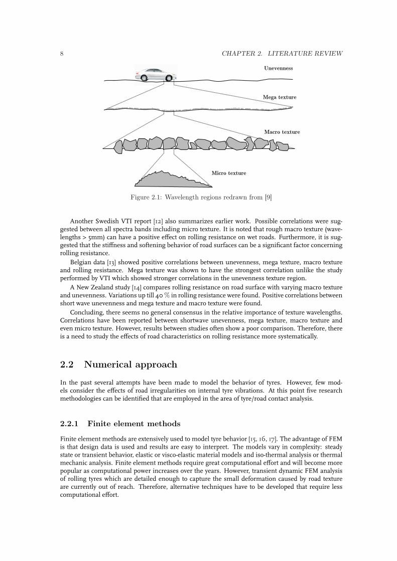
In the past, several attempts have been made to find correlations between road texture and rolling re-sistance. One of the problems in this respect is the characterization of road texture. Often a distinctionis made between different wavelengths regions as shows in Table 2.1.

Table 2.1: Wavelength regions

Name Wavelengths

Micro texture <0.5 [mm]Macro texture 0.5 - 50 [mm]Mega texture 0.05 - 0.5 [m]Unevenness 0.5 - 50 [m]

These texture regions are graphically illustrated in Fig. 2.1The SILVIA project [10], a European Commission Program, provides an interesting overview of

the empirical studies up till 2004. One of the first attempts to study the relationship between roadcharacteristics and rolling resistance was carried out by the Swedish National Road and TransportInstitute (VTI) in Sweden in the 1980th [11]. Texture profiles and fuel consumption were measured on20 different surfaces with constant speed (50-70 km/h). Positive correlations were observed betweenall texture wavelengths and fuel consumption. However, difficulties were found in identifying causalrelationships due to strong inter correlations between the different wavelengths. It is estimated thatthe shortwave unevenness can have an effect up to 10% in fuel economy. However, as the drivingspeed increases, smaller texture wavelengths increase in importance.

7

8 CHAPTER 2. LITERATURE REVIEW

Unevenness

Mega texture

Macro texture

Micro texture

Figure 2.1: Wavelength regions redrawn from [9]

Another Swedish VTI report [12] also summarizes earlier work. Possible correlations were sug-gested between all spectra bands including micro texture. It is noted that rough macro texture (wave-lengths > 5mm) can have a positive effect on rolling resistance on wet roads. Furthermore, it is sug-gested that the stiffness and softening behavior of road surfaces can be a significant factor concerningrolling resistance.

Belgian data [13] showed positive correlations between unevenness, mega texture, macro textureand rolling resistance. Mega texture was shown to have the strongest correlation unlike the studyperformed by VTI which showed stronger correlations in the unevenness texture region.

A New Zealand study [14] compares rolling resistance on road surface with varying macro textureand unevenness. Variations up till 40 % in rolling resistance were found. Positive correlations betweenshort wave unevenness and mega texture and macro texture were found.

Concluding, there seems no general consensus in the relative importance of texture wavelengths.Correlations have been reported between shortwave unevenness, mega texture, macro texture andeven micro texture. However, results between studies often show a poor comparison. Therefore, thereis a need to study the effects of road characteristics on rolling resistance more systematically.

2.2 Numerical approach

In the past several attempts have been made to model the behavior of tyres. However, few mod-els consider the effects of road irregularities on internal tyre vibrations. At this point five researchmethodologies can be identified that are employed in the area of tyre/road contact analysis.

2.2.1 Finite element methods

Finite element methods are extensively used to model tyre behavior [15, 16, 17]. The advantage of FEMis that design data is used and results are easy to interpret. The models vary in complexity: steadystate or transient behavior, elastic or visco-elastic material models and iso-thermal analysis or thermalmechanic analysis. Finite element methods require great computational effort and will become morepopular as computational power increases over the years. However, transient dynamic FEM analysisof rolling tyres which are detailed enough to capture the small deformation caused by road textureare currently out of reach. Therefore, alternative techniques have to be developed that require lesscomputational effort.

2.2. NUMERICAL APPROACH 9

2.2.2 Kropp et al.

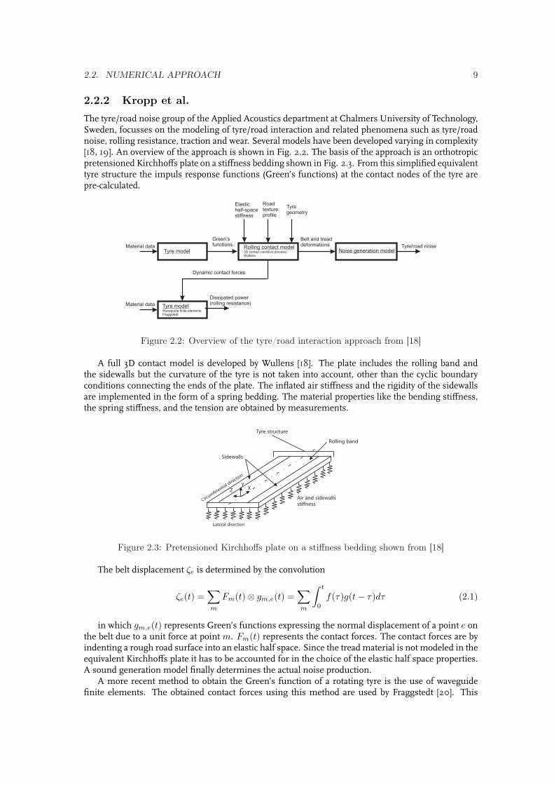
The tyre/road noise group of the Applied Acoustics department at Chalmers University of Technology,Sweden, focusses on the modeling of tyre/road interaction and related phenomena such as tyre/roadnoise, rolling resistance, traction and wear. Several models have been developed varying in complexity[18, 19]. An overview of the approach is shown in Fig. 2.2. The basis of the approach is an orthotropicpretensioned Kirchhoffs plate on a stiffness bedding shown in Fig. 2.3. From this simplified equivalenttyre structure the impuls response functions (Green’s functions) at the contact nodes of the tyre arepre-calculated.

Tyre modelRolling contact model3D contact (iterative process)Wullens

Tyre modelWaveguide finite elementsFraggstedt

Noise generation modelMaterial data

Material data

Green’sfunctions

Dynamic contact forces

Elastichalf-spacestiffness

Roadtextureprofile

Tyregeometry

Belt and treaddeformations Tyre/road noise

Dissipated power(rolling resistance)

Figure 2.2: Overview of the tyre/road interaction approach from [18]

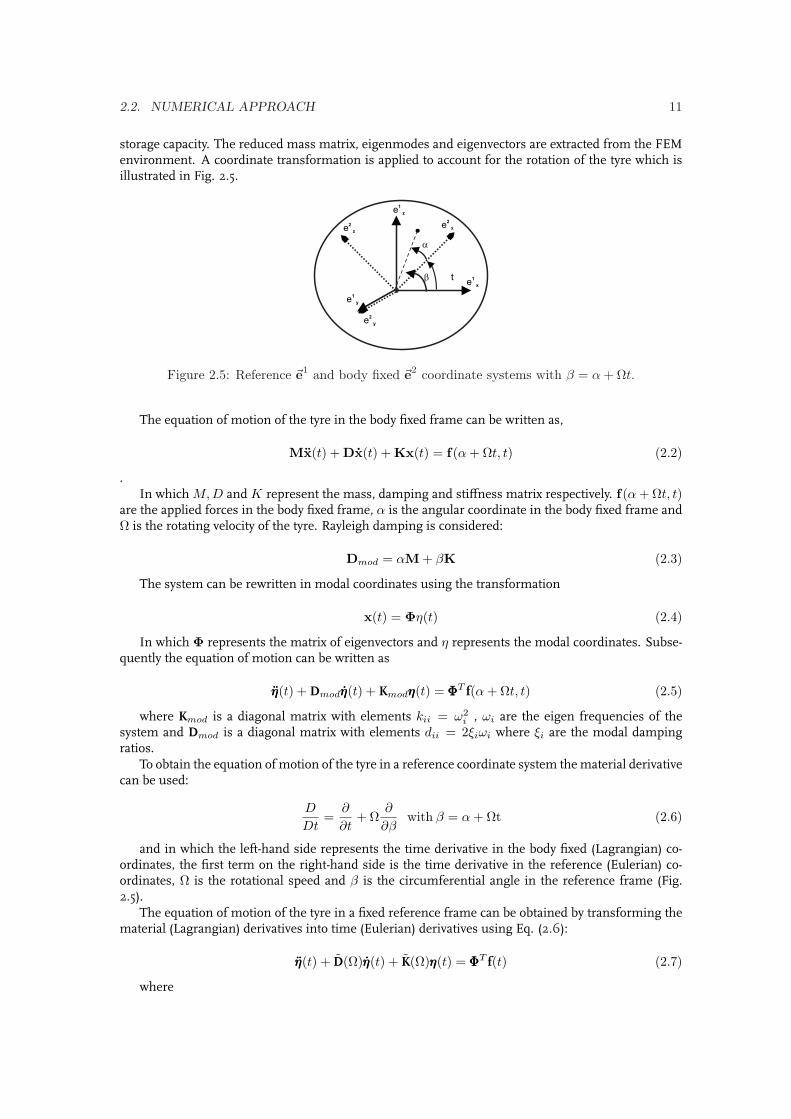
A full 3D contact model is developed by Wullens [18]. The plate includes the rolling band andthe sidewalls but the curvature of the tyre is not taken into account, other than the cyclic boundaryconditions connecting the ends of the plate. The inflated air stiffness and the rigidity of the sidewallsare implemented in the form of a spring bedding. The material properties like the bending stiffness,the spring stiffness, and the tension are obtained by measurements.

Rolling band

Sidewalls

Z

YX

Air and sidewallssti ness

Lateral direction

Circumferentialdirection

Tyre structure

Figure 2.3: Pretensioned Kirchhoffs plate on a stiffness bedding shown from [18]

The belt displacement ζe is determined by the convolution

ζe(t) =∑m

Fm(t)⊗ gm,e(t) =∑m

∫ t

0

f(τ)g(t− τ)dτ (2.1)

in which gm,e(t) represents Green’s functions expressing the normal displacement of a point e onthe belt due to a unit force at point m. Fm(t) represents the contact forces. The contact forces are byindenting a rough road surface into an elastic half space. Since the tread material is not modeled in theequivalent Kirchhoffs plate it has to be accounted for in the choice of the elastic half space properties.A sound generation model finally determines the actual noise production.

A more recent method to obtain the Green’s function of a rotating tyre is the use of waveguidefinite elements. The obtained contact forces using this method are used by Fraggstedt [20]. This


model predicts the energy dissipation of a tyre which is rolling on a rough road surface. The energydissipation is shown to be comparable to measurement results. The tyre dissipates more power on arough road surface than on a smooth road surface. The advantage of the model is that it shows theelements within the tyre with the highest energy dissipation. It is also shown that most of the energyis dissipated at frequencies below 250 Hz.

2.2.3 O’boy and Dowling

O’boy and Dowling [21, 22] at the engineering department at the University of Cambridge use a multilayer viscoelastic cylindrical representation of the tyre belt shown in Fig. 2.4 to determine the vibra-tion characteristics of a tyre. The parameters in the model are defined solely by design data. Thismodel of the tyre belt is then used to determine the parameters of an equivalent simple bending platemodel. From this result the Green’s functions for the contact nodes are determined using the sameapproach as at Chalmers University. The tyre is rolled over a textured road surface. The contact forcesare determined using the belt displacement, the undeformed tread block height and the tread blockstiffness. This method is used to predict tyre/road noise. Rolling resistance is not yet examined usingthis approach.

Figure 2.4: Complete viscoelastic cylindrical model of the tyre belt from [21]

2.2.4 Brinkmeier et al.

In Germany Brinkmeier et al. also aim at the prediction of rolling noise. However, finite elementmethods are used instead of simplified equivalent structures or waveguide finite elements [23]. AnArbitrary Lagrangian Eulerian (ALE) approach is employed to describe the steady state rolling ona smooth road surface [24]. This approach uses a reference frame that removes the explicit timedependence from the problem so that a purely spatially dependent analysis can be performed. Thischoice of reference frame allows the finite element mesh to remain stationary. Transfer functions aredetermined which relate a force input at the contact nodes to the tyre vibrations in a rotating tyre.

Finally, a linear tyre/road interaction model is defined in the frequency domain. A discrete Fourieranalysis of texture measurements results in a frequency spectrum. Using the contact patch stiffnessthis is transferred into an excitation function. By combining the transfer functions and excitation func-tions the tyre vibrations can be determined. Subsequently, a sound generation analysis is performed.However, there has been no attempt to study the energy dissipation due to the tyre vibrations.

2.2.5 Lopez et al.

At Eindhoven University of Technology a methodology to model tyre vibrations has been developed inrecent years [25, 26, 27]. In this approach, a transformation on the modal representation of a staticdeformed tyre is used to account for the rotation of the tyre.

First, the tyre is inflated and pressed against a smooth road surface and the highly nonlinearstationary tyre deformations are determined. A modal base is constructed around the deformed state.Subsequently, reduction techniques are applied to reduce the amount of computational effort and

2.2. NUMERICAL APPROACH 11

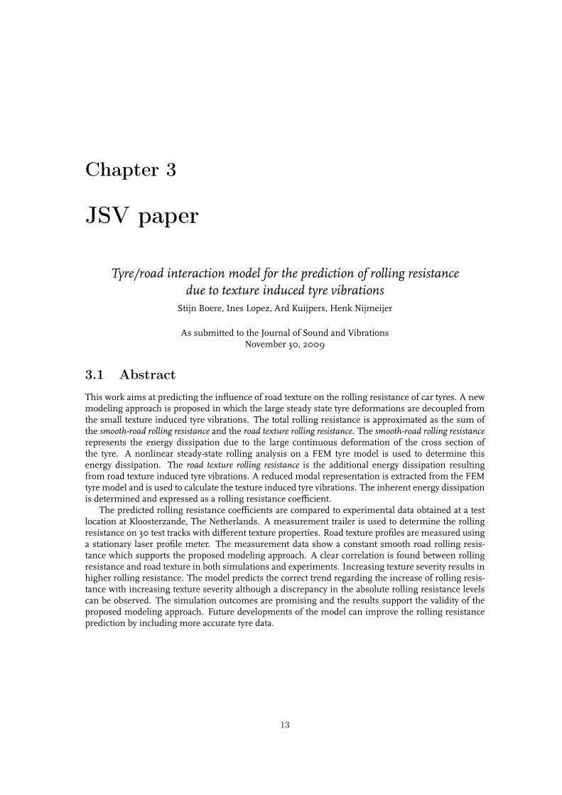
storage capacity. The reduced mass matrix, eigenmodes and eigenvectors are extracted from the FEMenvironment. A coordinate transformation is applied to account for the rotation of the tyre which isillustrated in Fig. 2.5.

e1

x

e2

x

e1

z

e2

z

b t

a

e1

y

e2

y

Figure 2.5: Reference ~e1 and body fixed ~e2 coordinate systems with β = α + Ωt.

The equation of motion of the tyre in the body fixed frame can be written as,

Mx(t) + Dx(t) + Kx(t) = f(α + Ωt, t) (2.2)

.In which M,D and K represent the mass, damping and stiffness matrix respectively. f(α + Ωt, t)

are the applied forces in the body fixed frame, α is the angular coordinate in the body fixed frame andΩ is the rotating velocity of the tyre. Rayleigh damping is considered:

Dmod = αM + βK (2.3)

The system can be rewritten in modal coordinates using the transformation

x(t) = Φη(t) (2.4)

In which Φ represents the matrix of eigenvectors and η represents the modal coordinates. Subse-quently the equation of motion can be written as

ηηη(t) + Dmodηηη(t) + Kmodηηη(t) = ΦΦΦT f(α + Ωt, t) (2.5)

where Kmod is a diagonal matrix with elements kii = ω2i , ωi are the eigen frequencies of the

system and Dmod is a diagonal matrix with elements dii = 2ξiωi where ξi are the modal dampingratios.

To obtain the equation of motion of the tyre in a reference coordinate system the material derivativecan be used:

D

Dt=

∂

∂t+ Ω

∂

∂βwith β = α + Ωt (2.6)

and in which the left-hand side represents the time derivative in the body fixed (Lagrangian) co-ordinates, the first term on the right-hand side is the time derivative in the reference (Eulerian) co-ordinates, Ω is the rotational speed and β is the circumferential angle in the reference frame (Fig.2.5).

The equation of motion of the tyre in a fixed reference frame can be obtained by transforming thematerial (Lagrangian) derivatives into time (Eulerian) derivatives using Eq. (2.6):

ηηη(t) + D(Ω)ηηη(t) + K(Ω)ηηη(t) = ΦΦΦT f(t) (2.7)

where


D = 2P(Ω, M,ΦΦΦ) + Dmod (2.8)

K = S(Ω, M,ΦΦΦ) + DmodP(Ω, M,ΦΦΦ) + Kmod (2.9)

The matrices S,P are added stiffness and damping terms due to the rotation:

P(Ω, M,ΦΦΦ) = ΦΦΦT (β)M(

ΩΩΩΦΦΦ(β) + Ω∂ΦΦΦ(β)

∂β

)(2.10)

S(Ω, M,ΦΦΦ) = ΦΦΦT (β)M(

ΩΩΩ2ΦΦΦ(β) + 2ΩΩΩΩ∂ΦΦΦ(β)

∂β+ Ω2 ∂2ΦΦΦ(β)

∂β2

)(2.11)

Equations (2.4) and (2.7) now give a the response of the tyre in a fixed reference frame. From thispoint either transfer function or Green’s function can be determined. The Green’s function’s can beused in a tyre/road interaction model.

An advantage of the approach at Eindhoven University of Technology is that it is solely based ondesign data in a FEM environment. Furthermore, the applied reduction techniques limit the requiredcomputational effort. Kersjes [28] has successfully combined the method of Lopez et al. with thetyre/road contact model of Wullens [18] to predict tyre vibrations. However, no attempts have yet beenmade to determine the energy dissipation due to these tyre vibrations.

2.2.6 Conclusion

The influence of road texture on rolling resistance is still rather unclear. Empirical studies do notalways agree and measurements are often unreliable and time consuming. Few numerical modelshave been designed to predict the influence of road texture on rolling resistance. A full finite elementanalysis requires great computational effort and is therefore still out of reach. The only existing modelwhich is able to predict rolling resistance on arbitrary road surfaces is the model of Fraggstedt [20].The current work focusses on extending the tyre/road noise model developed at Eindhoven Universityof Technology with a new rolling resistance prediction module.

Chapter 3

JSV paper

Tyre/road interaction model for the prediction of rolling resistancedue to texture induced tyre vibrations

Stijn Boere, Ines Lopez, Ard Kuijpers, Henk Nijmeijer

As submitted to the Journal of Sound and VibrationsNovember 30, 2009

3.1 Abstract

This work aims at predicting the influence of road texture on the rolling resistance of car tyres. A newmodeling approach is proposed in which the large steady state tyre deformations are decoupled fromthe small texture induced tyre vibrations. The total rolling resistance is approximated as the sum ofthe smooth-road rolling resistance and the road texture rolling resistance. The smooth-road rolling resistancerepresents the energy dissipation due to the large continuous deformation of the cross section ofthe tyre. A nonlinear steady-state rolling analysis on a FEM tyre model is used to determine thisenergy dissipation. The road texture rolling resistance is the additional energy dissipation resultingfrom road texture induced tyre vibrations. A reduced modal representation is extracted from the FEMtyre model and is used to calculate the texture induced tyre vibrations. The inherent energy dissipationis determined and expressed as a rolling resistance coefficient.

The predicted rolling resistance coefficients are compared to experimental data obtained at a testlocation at Kloosterzande, The Netherlands. A measurement trailer is used to determine the rollingresistance on 30 test tracks with different texture properties. Road texture profiles are measured usinga stationary laser profile meter. The measurement data show a constant smooth road rolling resis-tance which supports the proposed modeling approach. A clear correlation is found between rollingresistance and road texture in both simulations and experiments. Increasing texture severity results inhigher rolling resistance. The model predicts the correct trend regarding the increase of rolling resis-tance with increasing texture severity although a discrepancy in the absolute rolling resistance levelscan be observed. The simulation outcomes are promising and the results support the validity of theproposed modeling approach. Future developments of the model can improve the rolling resistanceprediction by including more accurate tyre data.

13

14 CHAPTER 3. JSV PAPER

3.2 Introduction

In Europe, 18% of the total CO2 emission originates from road transport [1]. Aerodynamic resistance,inertial forces, climbing forces and rolling resistance contribute to the total force a vehicle has toovercome to maintain constant speed. Rolling resistance is an important factor in this respect sinceit accounts for approximately 20-30 % to the energy consumption of a typical passenger car [3, 4].Lowering rolling resistance in pneumatic tyres can therefore greatly contribute to the reduction ofgreenhouse gas emissions.

Rolling resistance of pneumatic tyres has been the subject of extensive study in the past. Correla-tions with various parameters are found such as inflation pressure, tyre material properties and tyretemperature [5, 6, 7, 8]. Most of these studies use either experimental data, analytical derivations onequivalent structures or finite element method (FEM) analyses to predict rolling resistance. Road tex-ture is one of the parameters that has received less attention in the past. Instead, smooth road surfacesare used as an approximation which is probably due to the high computational effort involved in usingthe necessary detailed time domain FEM models.

In order to study the effects of road texture on rolling resistance a thorough understanding of tyreand contact dynamics is required. Existing literature on the influence of road texture on rolling re-sistance mainly uses experimental data to relate various texture metrics to the rolling resistance level.The SILVIA project [10] provides an interesting overview of the empirical work done up till 2004. Sig-nificant increases in rolling resistance and fuel consumption are found for increasing texture severity[11, 13]. No general consensus can be found on the relative importance of different texture wavelengthbands. Moreover, rolling resistance often shows a poor measurement reproducibility. Therefore, thispaper proposes a modeling approach to study the effects of road texture on rolling resistance moresystematically.

A variety of tyre models have been developed to analyze vehicle handling, comfort and tyre wear[29, 30]. Few models are able to predict the effect of road irregularities [31]. Models that do considerthe effects of road texture often aim at the prediction of tyre/road noise. The relevant frequenciesconcerning tyre/road noise are approximately 0.3-2 kHz. These frequencies are much higher than thefrequencies that influence rolling resistance, 0 − 300 Hz [21, 20]. Many of the existing dynamic tyremodels are based on equivalent tyre structures such as plates and rings [19, 32, 33]. The parametersin these equivalent structure models have to be determined through a comparison with experimentaldata. This limits the use of these simplified models since every new tyre design needs prototyping inorder to find the appropriate model parameters.

An alternative approach is the use of finite element methods to model the dynamic behavior ofthe tyre. The advantage of FEM above equivalent structure methods is that representative design datais used. This allows the tyre manufacturer to assess the dynamic tyre properties without prototyping.However, due to the large number of degrees of freedom, a full scale FEM analysis requires greatcomputational effort. Therefore, a time domain analysis using FEM is still out of reach. A time inde-pendent solution can be obtained by a steady state rolling analysis which uses an Arbitrary LagrangianEulerian formulation (ALE) [24, 23]. A steady-state rolling analysis allows for local mesh refinementof the contact region which is essential for accurate contact analysis. However, a steady state rollinganalysis can only be performed on an axi-symmetric tyre. Therefore, it is not possible to include treadblocks. Furthermore, the effects of road texture can not be taken into account since a smooth roadsurface is required.

This work focuses on texture induced tyre vibrations and the inherent energy dissipation whichcontributes to the total rolling resistance. The goal of this paper is to predict the influence of roadtexture on rolling resistance. A new computationally efficient modeling approach is proposed in whichthe large steady state tyre deformations are decoupled from the small texture induced tyre vibrations.The total rolling resistance is approximated as the sum of the smooth-road rolling resistance and the roadtexture rolling resistance. The two parts of the rolling resistance are analyzed separately. The smooth-road rolling resistance is the energy dissipation due to the continuous deformation of the cross sectionof the tyre. A nonlinear steady-state rolling analysis on a FEM tyre model is used to determine thisenergy dissipation. The road texture rolling resistance is the additional energy dissipation resulting fromroad texture induced tyre vibrations. A reduced modal representation is extracted from the FEM tyre

3.3. MODELING APPROACH 15

description. This modal representation is used as a boundary impedance condition in a tyre/roadinteraction model.

This paper is organized as follows: in Section 3.3 the modeling approach is discussed in detail.The smooth-road rolling resistance is analyzed in Section 3.4. The road texture rolling resistance isanalyzed using a tyre/road interaction model which is presented in Section 3.5. The results of thetyre/road interaction model are compared to results found in literature in Section 3.6. A comparisonof the numerical results with measurements is given in Section 3.7. In Section 3.8 conclusions aredrawn and future work is discussed.

3.3 Modeling approach

There are a number of definitions of rolling resistance: it can be expressed as either a resisting force atthe wheel axle, a resisting moment around the wheel axle or a power dissipation. To avoid confusion,an accurate definition of rolling resistance is important. Rolling resistance can be defined as the powerdissipation Pdis at a certain axle load Naxle. The power dissipation depends on the resistant force Fres

acting on the wheel axle and the vehicle velocity v. In this study, the rolling resistance coefficient,RRC, is used to quantify rolling resistance:

RRC =Fres

Naxle=

Pdis

Naxlev. (3.1)

It has been shown that the resistant force Fres is linearly dependent on the applied axle loadNaxle in the practical range of axle loads [4]. Therefore, the rolling resistance coefficient does notchange with changing axle loads. Furthermore, the rolling resistance coefficient has been shown tobe fairly constant with increasing velocity [13]. This simplifies the comparison between results foundin literature. Rolling resistance coefficients generally range from 0.006 to 0.013 for tyres on modernpassenger cars [4].

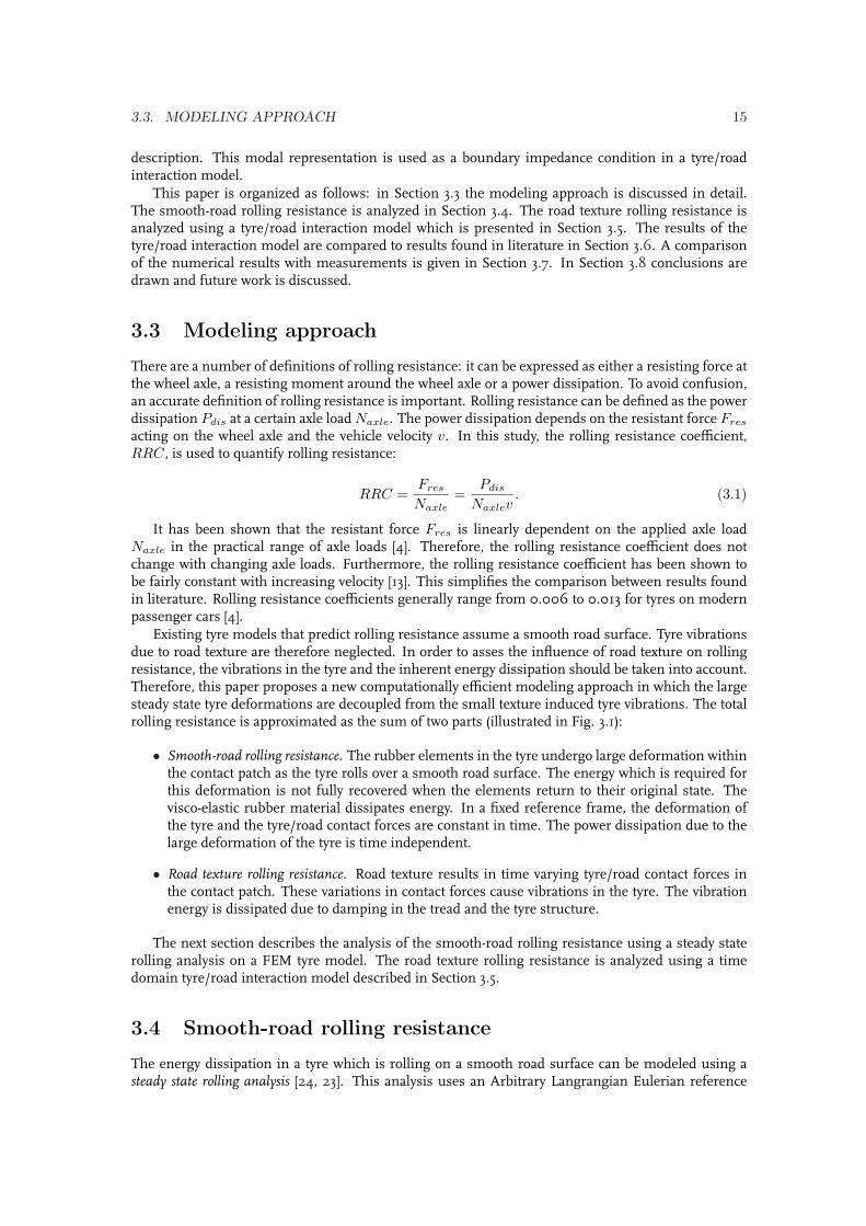
Existing tyre models that predict rolling resistance assume a smooth road surface. Tyre vibrationsdue to road texture are therefore neglected. In order to asses the influence of road texture on rollingresistance, the vibrations in the tyre and the inherent energy dissipation should be taken into account.Therefore, this paper proposes a new computationally efficient modeling approach in which the largesteady state tyre deformations are decoupled from the small texture induced tyre vibrations. The totalrolling resistance is approximated as the sum of two parts (illustrated in Fig. 3.1):

• Smooth-road rolling resistance. The rubber elements in the tyre undergo large deformation withinthe contact patch as the tyre rolls over a smooth road surface. The energy which is required forthis deformation is not fully recovered when the elements return to their original state. Thevisco-elastic rubber material dissipates energy. In a fixed reference frame, the deformation ofthe tyre and the tyre/road contact forces are constant in time. The power dissipation due to thelarge deformation of the tyre is time independent.

• Road texture rolling resistance. Road texture results in time varying tyre/road contact forces inthe contact patch. These variations in contact forces cause vibrations in the tyre. The vibrationenergy is dissipated due to damping in the tread and the tyre structure.

The next section describes the analysis of the smooth-road rolling resistance using a steady staterolling analysis on a FEM tyre model. The road texture rolling resistance is analyzed using a timedomain tyre/road interaction model described in Section 3.5.

3.4 Smooth-road rolling resistance

The energy dissipation in a tyre which is rolling on a smooth road surface can be modeled using asteady state rolling analysis [24, 23]. This analysis uses an Arbitrary Langrangian Eulerian reference


(b) c)(a) (

Figure 3.1: Schematic representation of the proposed modeling approach. (a) Base state (b) Thesmooth-road rolling resistance resulting from steady state tyre deformations. (c) The road texturerolling resistance due to texture induced tyre vibrations.

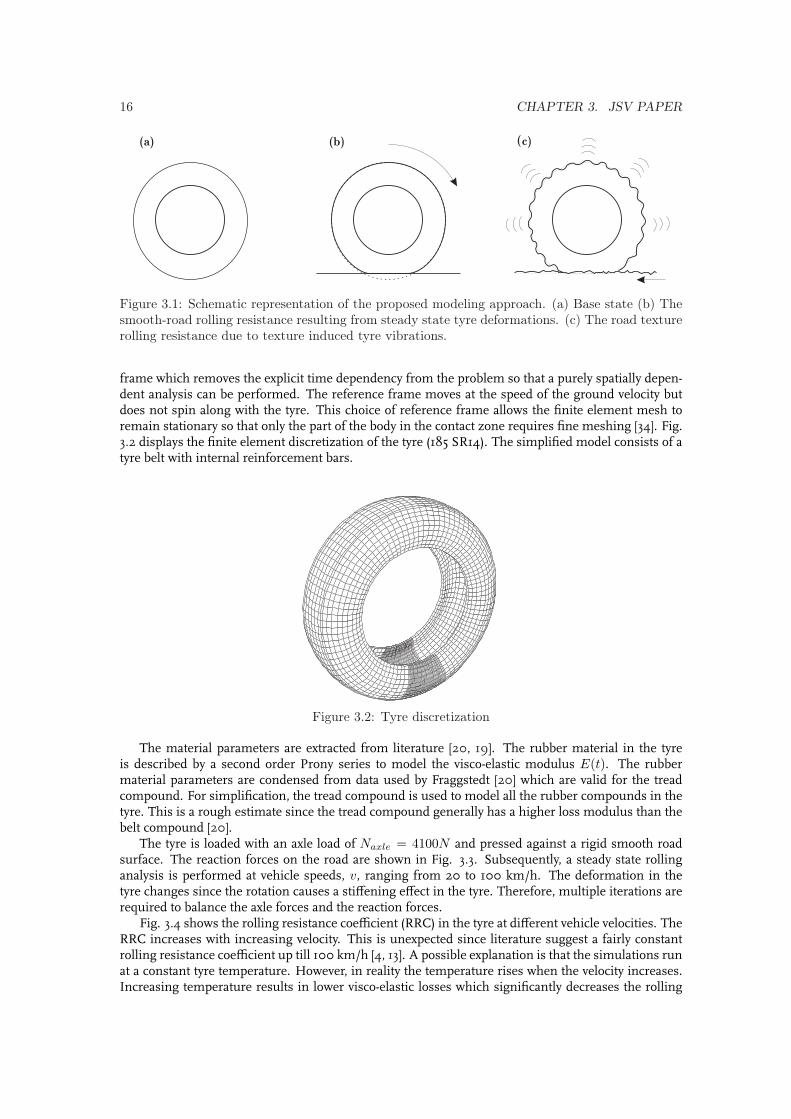
frame which removes the explicit time dependency from the problem so that a purely spatially depen-dent analysis can be performed. The reference frame moves at the speed of the ground velocity butdoes not spin along with the tyre. This choice of reference frame allows the finite element mesh toremain stationary so that only the part of the body in the contact zone requires fine meshing [34]. Fig.3.2 displays the finite element discretization of the tyre (185 SR14). The simplified model consists of atyre belt with internal reinforcement bars.

Figure 3.2: Tyre discretization

The material parameters are extracted from literature [20, 19]. The rubber material in the tyreis described by a second order Prony series to model the visco-elastic modulus E(t). The rubbermaterial parameters are condensed from data used by Fraggstedt [20] which are valid for the treadcompound. For simplification, the tread compound is used to model all the rubber compounds in thetyre. This is a rough estimate since the tread compound generally has a higher loss modulus than thebelt compound [20].

The tyre is loaded with an axle load of Naxle = 4100N and pressed against a rigid smooth roadsurface. The reaction forces on the road are shown in Fig. 3.3. Subsequently, a steady state rollinganalysis is performed at vehicle speeds, v, ranging from 20 to 100 km/h. The deformation in thetyre changes since the rotation causes a stiffening effect in the tyre. Therefore, multiple iterations arerequired to balance the axle forces and the reaction forces.

Fig. 3.4 shows the rolling resistance coefficient (RRC) in the tyre at different vehicle velocities. TheRRC increases with increasing velocity. This is unexpected since literature suggest a fairly constantrolling resistance coefficient up till 100 km/h [4, 13]. A possible explanation is that the simulations runat a constant tyre temperature. However, in reality the temperature rises when the velocity increases.Increasing temperature results in lower visco-elastic losses which significantly decreases the rolling

3.4. SMOOTH-ROAD ROLLING RESISTANCE 17

Contact force, Magnitude [N]

+0.000e+00

+4.949e+00

+9.899e+00

+1.485e+01

+1.980e+01

+2.475e+01

+2.970e+01

+3.465e+01

+3.960e+01

+4.454e+01

+4.949e+01

+5.444e+01

+5.939e+01

Figure 3.3: Contact force distribution for a tyre load of 4100 N

resistance coefficient [13].

At 80 km/h the RRC equals approximately 0.0135. This exceeds the expected values reported inliterature [4]. This could either be a result of the mismatched temperature or the relatively high lossmodulus of the tyre tread compound which is used to model all the rubber compounds in the tyre. Inthe future, the steady state rolling analysis can be used on improved FEM models which include moreaccurate tyre data and temperature effects.

0 20 40 60 80 100 1200

0.002

0.004

0.006

0.008

0.01

0.012

0.014

0.016

Vehicle velocity [km/h]

Rollin

g r

esis

tance

coe

ffic

ient

[-]

Figure 3.4: Rolling resistance coefficient as a function of vehicle velocity

There is little computational effort involved in computing the smooth-road rolling resistance sincethe mesh remains stationary and only the contact patch requires a fine discretization. However, asteady state rolling analysis can only be performed on an axi-symmetric tyre. Therefore, it is not pos-sible to include tread blocks. Furthermore, since this analysis is time independent it is not possible topredict road texture induced tyre vibrations. In the next section the road texture rolling resistance isanalyzed using a tyre/road interaction model. The basis of the interaction model is a modal represen-tation of the same FEM model as presented in this section. The tread blocks are modeled as separatesubsystems since they are not included in the FEM model.


3.5 Road texture rolling resistance

Due to nonlinear phenomena such as the varying size of the contact patch, a tyre/road interactionmodel has to be represented in the time domain. Tyre/road interaction models often use Winklerbeddings or elastic half spaces to describe the contact characteristics between the tyre belt and theroad [35, 18]. In this work, a tyre/road interaction model is developed which is based on the approachby Andersson and Kropp [36]. The advantage of this approach is that it accounts for small wavelengthroad texture by applying a nonlinear contact stiffness to the road.

Fig. 3.5 presents a schematic overview of the tyre/road interaction model.

Dynamic response of deformed rotating tyre

Tread dynamics

Contact stiffness

Figure 3.5: Schematic overview of the tyre/road model

The model consists of three layers:

• Dynamic response of the deformed rotating tyre: Green’s functions are used to represent thedeformed rotating tyre. These Green’s functions serve as a boundary impedance condition.

• Tread dynamics: The tread dynamics are modeled using a linear spring damper system.

• Contact mechanics: The contact mechanics between the tread blocks and the road surface aremodeled using a nonlinear stiffness function which accounts for the indentation of the treadblock by the road asperities.

Fig. 3.6 shows the components of a contact subsystem in detail. The two degrees of freedom[x1(t), x2(t)] represent the position of the lowest point on the tread block and the position of the tyrebelt respectively. Furthermore, p(t) represents the height of the road profile and z1 and z2 representthe rest positions of the tread blocks and belt respectively. The initial forces Finit are imported fromthe FEM analysis and are shown in Fig. 3.3.

x (t)2

x (t)1

p(t)

z1

z2

f(p-z -x )1 1

kld

Green sfunctions

’

Finit

Figure 3.6: Graphical representation of a contact subsystem

3.5. ROAD TEXTURE ROLLING RESISTANCE 19

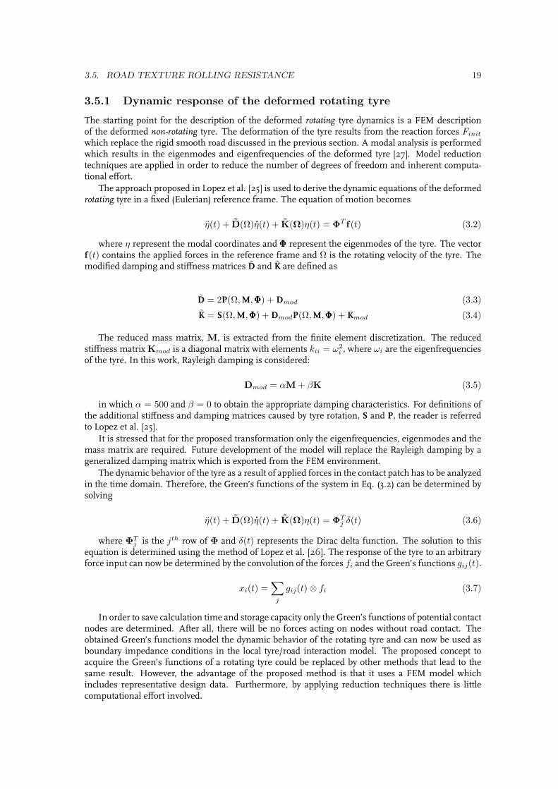
3.5.1 Dynamic response of the deformed rotating tyre

The starting point for the description of the deformed rotating tyre dynamics is a FEM descriptionof the deformed non-rotating tyre. The deformation of the tyre results from the reaction forces Finit

which replace the rigid smooth road discussed in the previous section. A modal analysis is performedwhich results in the eigenmodes and eigenfrequencies of the deformed tyre [27]. Model reductiontechniques are applied in order to reduce the number of degrees of freedom and inherent computa-tional effort.

The approach proposed in Lopez et al. [25] is used to derive the dynamic equations of the deformedrotating tyre in a fixed (Eulerian) reference frame. The equation of motion becomes

η(t) + D(Ω)η(t) + K(Ω)η(t) = ΦT f(t) (3.2)

where η represent the modal coordinates and ΦΦΦ represent the eigenmodes of the tyre. The vectorf(t) contains the applied forces in the reference frame and Ω is the rotating velocity of the tyre. Themodified damping and stiffness matrices D and K are defined as

D = 2P(Ω, M,ΦΦΦ) + Dmod (3.3)

K = S(Ω, M,ΦΦΦ) + DmodP(Ω, M,ΦΦΦ) + Kmod (3.4)

The reduced mass matrix, M, is extracted from the finite element discretization. The reducedstiffness matrix Kmod is a diagonal matrix with elements kii = ω2

i , where ωi are the eigenfrequenciesof the tyre. In this work, Rayleigh damping is considered:

Dmod = αM + βK (3.5)

in which α = 500 and β = 0 to obtain the appropriate damping characteristics. For definitions ofthe additional stiffness and damping matrices caused by tyre rotation, S and P, the reader is referredto Lopez et al. [25].

It is stressed that for the proposed transformation only the eigenfrequencies, eigenmodes and themass matrix are required. Future development of the model will replace the Rayleigh damping by ageneralized damping matrix which is exported from the FEM environment.

The dynamic behavior of the tyre as a result of applied forces in the contact patch has to be analyzedin the time domain. Therefore, the Green’s functions of the system in Eq. (3.2) can be determined bysolving

η(t) + D(Ω)η(t) + K(Ω)η(t) = ΦTj δ(t) (3.6)

where ΦTj is the jth row of Φ and δ(t) represents the Dirac delta function. The solution to this

equation is determined using the method of Lopez et al. [26]. The response of the tyre to an arbitraryforce input can now be determined by the convolution of the forces fi and the Green’s functions gij(t).

xi(t) =∑

j

gij(t)⊗ fi (3.7)

In order to save calculation time and storage capacity only the Green’s functions of potential contactnodes are determined. After all, there will be no forces acting on nodes without road contact. Theobtained Green’s functions model the dynamic behavior of the rotating tyre and can now be used asboundary impedance conditions in the local tyre/road interaction model. The proposed concept toacquire the Green’s functions of a rotating tyre could be replaced by other methods that lead to thesame result. However, the advantage of the proposed method is that it uses a FEM model whichincludes representative design data. Furthermore, by applying reduction techniques there is littlecomputational effort involved.


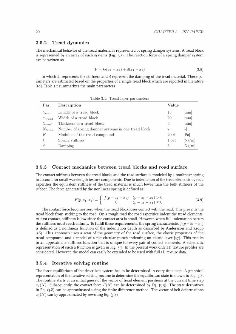
3.5.2 Tread dynamics

The mechanical behavior of the tread material is represented by spring damper systems. A tread blockis represented by an array of such systems (Fig. 3.5). The reaction force of a spring damper systemcan be written as

F = kl(x1 − x2) + d(x1 − x2) (3.8)

in which kl represents the stiffness and d represent the damping of the tread material. These pa-rameters are estimated based on the properties of a single tread block which are reported in literature[19]. Table 3.1 summarizes the main parameters

Table 3.1: Tread layer parameters

Par. Description Value

ltread Length of a tread block 15 [mm]wtread Width of a tread block 20 [mm]ttread Thickness of a tread block 6 [mm]Ntread Number of spring damper systems in one tread block 7 [-]E Modulus of the tread compound 20e6 [Pa]kl Spring stiffness 1.5e5 [Ns/m]d Damping 5 [Ns/m]

3.5.3 Contact mechanics between tread blocks and road surface

The contact stiffness between the tread blocks and the road surface is modeled by a nonlinear springto account for small wavelength texture components. Due to indentation of the tread elements by roadasperities the equivalent stiffness of the tread material is much lower than the bulk stiffness of therubber. The force generated by the nonlinear spring is defined as:

F (p, z1, x1) =

f(p− z1 − x1) (p− z1 − x1) > 00 (p− z1 − x1) ≤ 0 (3.9)

The contact force becomes zero when the tread block loses contact with the road. This prevents thetread block from sticking to the road. On a rough road the road asperities indent the tread elements.At first contact, stiffness is low since the contact area is small. However, when full indentation occursthe stiffness must reach infinity. To fulfill these requirements, the spring characteristic f(p− z1−x1)is defined as a nonlinear function of the indentation depth as described by Andersson and Kropp[36]. This approach uses a scan of the geometry of the road surface, the elastic properties of thetread compound and a model of a flat circular punch indenting an elastic layer [37]. This resultsin an approximate stiffness function that is unique for every pair of contact elements. A schematicrepresentation of such a function is given in Fig. 3.7. In the present work only 2D texture profiles areconsidered. However, the model can easily be extended to be used with full 3D texture data.

3.5.4 Iterative solving routine

The force equilibrium of the described system has to be determined in every time step. A graphicalrepresentation of the iterative solving routine to determine the equilibrium state is shown in Fig. 3.8.The routine starts at an initial guess of the vector of tread element positions at the current time stepx1(N). Subsequently, the contact force F (N) can be determined by Eq. (3.9). The state derivativesin Eq. (3.8) can be approximated using the finite difference method. The vector of belt deformationsx2(N) can by approximated by rewriting Eq. (3.8)

3.5. ROAD TEXTURE ROLLING RESISTANCE 21

Indentation of road surface

Contact force

treadblock

treadblock Full indetatio

n

Figure 3.7: Schematic representation of the nonlinear function between the contact force and theindentation of the road surface

x1

F

Update

x1

x2

B

x2

A

+ -

Error

Figure 3.8: Graphical representation of the iterative simulation process

xA2 (N) ∼= d(x1(N)− x1(N − 1))− F (N)δt + dx2(N − 1) + δtklx1(N)

d + δtkl(3.10)

in which δt represents the time step. Alternatively, the deformation of the belt can be determinedby the convolution integral of the contact forces with the Green’s function in Eq. (B.2). This can beapproximated in discrete time by

xB2 (N) ∼= F (N)g(1)∆t +

N−1∑n=1

F (n)g(N − n + 1)∆t (3.11)

in which g(N) represents the discretized Green’s function at time point N.This results in an error between the displacements in Eqs. (3.10) and (B.2), |xA

2 (N) − xB2 (N)|,

which should be minimized to find the solution of the problem. Therefore, the sum of squared errorsis determined. Subsequently, the algorithm updates the initial guess of positions x1 and iterates untilthe squared error meets the desired solution criterion. For this iterative routine the nonlinear leastsquare solver in MATLAB is used.

A graphical representation of the simulation in subsequent time steps is given in Fig. 3.9. Everytime step, the road shifts nt number of elements forward. This results in a time step δt


δt = ntδx

v(3.12)

in which v represents the forward velocity of the vehicle and δx represent the length of an element.The tread blocks move along with the road. New (undeformed) tread blocks enter at the leading edge.Tread blocks leave the contact patch at the trailing edge. The voids in between tread blocks are modeledas tread elements with a zero stiffness.

t =1¢±t

n n-1 n-2 n-3 n-4 n-5 n-6n+1

n+2

n+3

n+4

n-8n-9

n-10

n-7

t =2¢±t

n n-1 n-2 n-3 n-4 n-5 n-6

n+2

n+3

n+4

n-8n-

9

n-10

n-7n+1

t =3¢±t

n n-1 n-2 n-3n-4 n-5 n-6

n+2

n+3

n+4

n-8n-

9n-

10

n-7n+1

Figure 3.9: Graphical representation of the simulation in subsequent time steps

The proposed numerical procedure is carried out during multiple rotations of the tyre. Duringinitialization of the simulation the sum of contact forces is monitored. If necessary, the indentationof the road p(t) is increased to match the desired axle load Naxle. The simulations show good con-vergence although on rough road surfaces more iterations are needed. Nevertheless, the simulationsrequire an acceptable computational effort.

3.5.5 Road texture rolling resistance

The road texture rolling resistance can now be determined using the obtained force and displacement

Pdis =Cn∑

i=1

1t2 − t1

∫ t2

t1

F i(t)xi1(t)dt (3.13)

3.6. MODEL VALIDATION 23

in which the time interval < t1, t2 > represents the time of one tyre revolution in which theaveraged total contact force has converged to the desired load. Furthermore, Cn represent the totalnumber of contact nodes in the contact patch. The starting time t1 is chosen such that transient effectsfrom axle load changes have faded out.

3.6 Model validation

The simulation results presented in this section correspond to a tyre load of 4100 N and a travelingvelocity of 80 km/h.

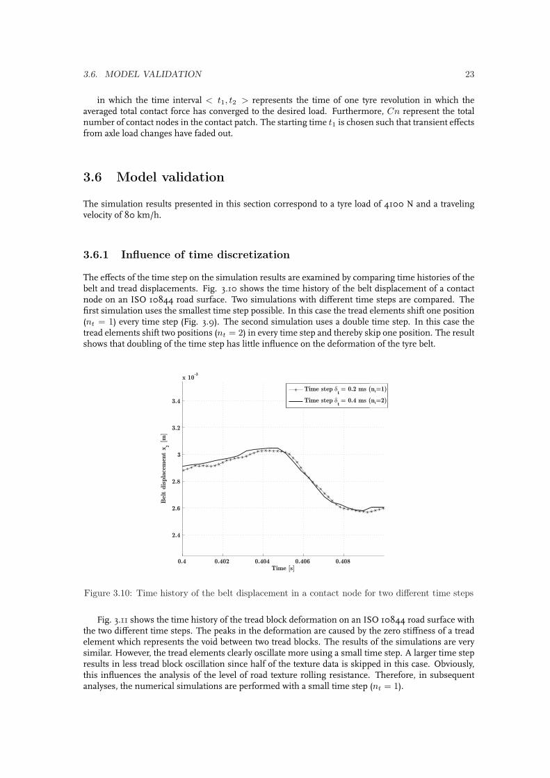
3.6.1 Influence of time discretization

The effects of the time step on the simulation results are examined by comparing time histories of thebelt and tread displacements. Fig. 3.10 shows the time history of the belt displacement of a contactnode on an ISO 10844 road surface. Two simulations with different time steps are compared. Thefirst simulation uses the smallest time step possible. In this case the tread elements shift one position(nt = 1) every time step (Fig. 3.9). The second simulation uses a double time step. In this case thetread elements shift two positions (nt = 2) in every time step and thereby skip one position. The resultshows that doubling of the time step has little influence on the deformation of the tyre belt.

0.4 0.402 0.404 0.406 0.408

2.4

2.6

2.8

3

3.2

3.4

x 10-3

Time [s]

Bel

t dis

pla

cem

ent

x 2[m

]

Time step δt= 0.2 ms (n =1)t


Figure 3.10: Time history of the belt displacement in a contact node for two different time steps

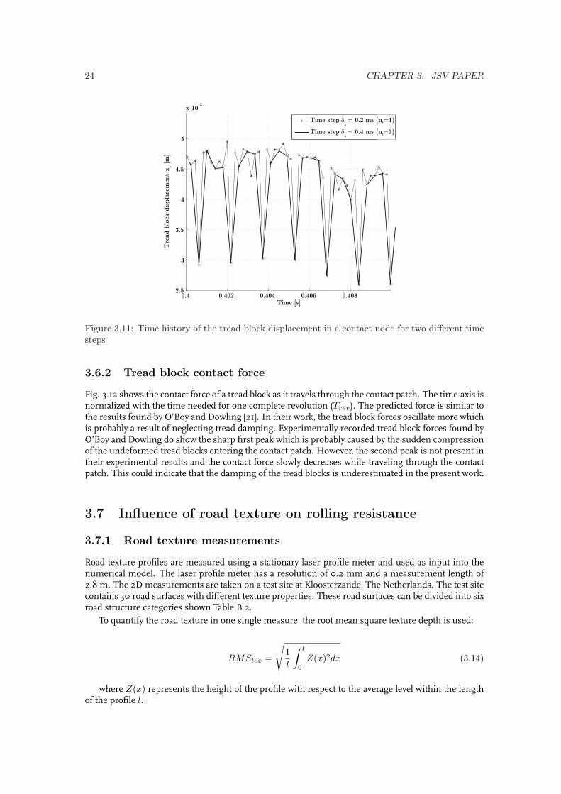
Fig. 3.11 shows the time history of the tread block deformation on an ISO 10844 road surface withthe two different time steps. The peaks in the deformation are caused by the zero stiffness of a treadelement which represents the void between two tread blocks. The results of the simulations are verysimilar. However, the tread elements clearly oscillate more using a small time step. A larger time stepresults in less tread block oscillation since half of the texture data is skipped in this case. Obviously,this influences the analysis of the level of road texture rolling resistance. Therefore, in subsequentanalyses, the numerical simulations are performed with a small time step (nt = 1).


0.4 0.402 0.404 0.406 0.4082.5

3

3.5

4

4.5

5

x 10-3

Time [s]

Tre

ad b

lock

dis

pla

cem

ent

x 1[m

]



Figure 3.11: Time history of the tread block displacement in a contact node for two different timesteps

3.6.2 Tread block contact force

Fig. 3.12 shows the contact force of a tread block as it travels through the contact patch. The time-axis isnormalized with the time needed for one complete revolution (Trev). The predicted force is similar tothe results found by O’Boy and Dowling [21]. In their work, the tread block forces oscillate more whichis probably a result of neglecting tread damping. Experimentally recorded tread block forces found byO’Boy and Dowling do show the sharp first peak which is probably caused by the sudden compressionof the undeformed tread blocks entering the contact patch. However, the second peak is not present intheir experimental results and the contact force slowly decreases while traveling through the contactpatch. This could indicate that the damping of the tread blocks is underestimated in the present work.

3.7 Influence of road texture on rolling resistance

3.7.1 Road texture measurements

Road texture profiles are measured using a stationary laser profile meter and used as input into thenumerical model. The laser profile meter has a resolution of 0.2 mm and a measurement length of2.8 m. The 2D measurements are taken on a test site at Kloosterzande, The Netherlands. The test sitecontains 30 road surfaces with different texture properties. These road surfaces can be divided into sixroad structure categories shown Table B.2.

To quantify the road texture in one single measure, the root mean square texture depth is used:

RMStex =

√1l

∫ l

0

Z(x)2dx (3.14)

where Z(x) represents the height of the profile with respect to the average level within the lengthof the profile l.

3.7. INFLUENCE OF ROAD TEXTURE ON ROLLING RESISTANCE 25

1.9 1.92 1.94 1.96 1.98 2 2.02 2.04 2.06 2.08 2.10

50

100

150

200

250

Time/Trev

Con

tact

For

ce [N

]

Figure 3.12: Contact force on a tread block traveling through the contact patch

Table 3.2: Road structure categories

Pavement type Designation

ISO10844 standardized road surface ISOStone Mastic Asphalt SMADense Asphalt Concrete DACThin Layered Asphalt TLASingle layer Porous Asphalt Concrete PACDouble layer Porous Asphalt Concrete DPAC

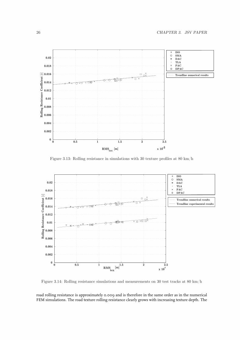
3.7.2 Influence of road texture on total rolling resistance

Numerical simulations on the 30 texture profiles are carried out to determine the road texture rollingresistance. The smooth-road rolling resistance remains constant on all surfaces. Fig. 3.13 shows therolling resistance coefficient (RRC) as a function of the texture depth RMStex.

There is a clear correlation between road texture and rolling resistance. Rolling resistance increaseslinearly with texture depth. A decrease in RMStex of 1mm results in a decrease in rolling resistanceof approximately 7%.

3.7.3 Rolling resistance measurements

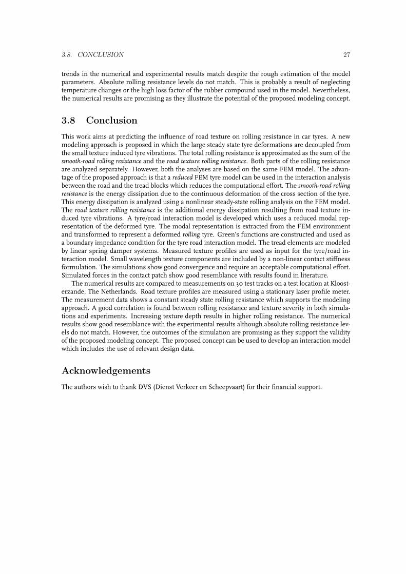
The numerical results are compared to measurements performed on a test site at Kloosterzande, TheNetherlands. The rolling resistance is measured using a trailer from the University of Gdansk, Poland.This trailer measures the ratio between the rolling resistance force and the axle force, i.e. the rollingresistance coefficient RRC. The trailer is equipped with a Continental 225/60 R16 test tyre. Themeasurements are taken at a velocity of 80 km/h and an axle load of 4100 kg. Fig. 3.14 showsthe total rolling resistance on 30 different road surfaces in both the numerical simulations and theexperimental measurements.

The measurements clearly indicate the presence of a smooth-road rolling resistance and a roadtexture rolling resistance. This observation supports the proposed modeling approach. The smooth-


0 0.5 1 1.5 2 2.5

x 10-3

0

0.002

0.004

0.006

0.008

0.01

0.012

0.014

0.016

0.018

0.02

RMStex

[m]

Rol

ling

Res

ista

nce

Coef

fici

ent

[-]

Trendline numerical results

ISOSMADACTLAPACDPAC

Figure 3.13: Rolling resistance in simulations with 30 texture profiles at 80 km/h

0 0.5 1 1.5 2 2.5

x 10-3

0

0.002

0.004

0.006

0.008

0.01

0.012

0.014

0.016

0.018

0.02

RMStex

[m]

Rol

ling

Res

ista

nce

Coef

fici

ent

[-]

ISOSMADACTLAPACDPAC

Trendline numerical results

Trendline experimental results

Figure 3.14: Rolling resistance simulations and measurements on 30 test tracks at 80 km/h

road rolling resistance is approximately 0.009 and is therefore in the same order as in the numericalFEM simulations. The road texture rolling resistance clearly grows with increasing texture depth. The

3.8. CONCLUSION 27

trends in the numerical and experimental results match despite the rough estimation of the modelparameters. Absolute rolling resistance levels do not match. This is probably a result of neglectingtemperature changes or the high loss factor of the rubber compound used in the model. Nevertheless,the numerical results are promising as they illustrate the potential of the proposed modeling concept.

3.8 Conclusion

This work aims at predicting the influence of road texture on rolling resistance in car tyres. A newmodeling approach is proposed in which the large steady state tyre deformations are decoupled fromthe small texture induced tyre vibrations. The total rolling resistance is approximated as the sum of thesmooth-road rolling resistance and the road texture rolling resistance. Both parts of the rolling resistanceare analyzed separately. However, both the analyses are based on the same FEM model. The advan-tage of the proposed approach is that a reduced FEM tyre model can be used in the interaction analysisbetween the road and the tread blocks which reduces the computational effort. The smooth-road rollingresistance is the energy dissipation due to the continuous deformation of the cross section of the tyre.This energy dissipation is analyzed using a nonlinear steady-state rolling analysis on the FEM model.The road texture rolling resistance is the additional energy dissipation resulting from road texture in-duced tyre vibrations. A tyre/road interaction model is developed which uses a reduced modal rep-resentation of the deformed tyre. The modal representation is extracted from the FEM environmentand transformed to represent a deformed rolling tyre. Green’s functions are constructed and used asa boundary impedance condition for the tyre road interaction model. The tread elements are modeledby linear spring damper systems. Measured texture profiles are used as input for the tyre/road in-teraction model. Small wavelength texture components are included by a non-linear contact stiffnessformulation. The simulations show good convergence and require an acceptable computational effort.Simulated forces in the contact patch show good resemblance with results found in literature.

The numerical results are compared to measurements on 30 test tracks on a test location at Kloost-erzande, The Netherlands. Road texture profiles are measured using a stationary laser profile meter.The measurement data shows a constant steady state rolling resistance which supports the modelingapproach. A good correlation is found between rolling resistance and texture severity in both simula-tions and experiments. Increasing texture depth results in higher rolling resistance. The numericalresults show good resemblance with the experimental results although absolute rolling resistance lev-els do not match. However, the outcomes of the simulation are promising as they support the validityof the proposed modeling concept. The proposed concept can be used to develop an interaction modelwhich includes the use of relevant design data.

Acknowledgements

The authors wish to thank DVS (Dienst Verkeer en Scheepvaart) for their financial support.

Chapter 4

Conclusions and Recommendations

4.1 Conclusions

This work extends the tyre/road noise model developed at Eindhoven University of Technology witha rolling resistance prediction module. A new three dimensional tyre/road interaction model is im-plemented which is able to account for small wavelength road texture. The energy dissipation is de-termined for several different road surfaces. The numerical results are compared to rolling resistancemeasurements. The main conclusions of this project are:

• The influence of road texture on rolling resistance is still rather unclear in literature. Empiricalstudies do not always agree and measurements are often unreliable and time consuming. Thereseems to be no general consensus in the relative importance of different texture wavelengthregions. Therefore, there is a need to study the effects of road characteristics on rolling resistancemore systematically. Since a full scale FEM analysis requires great computational effort, moreefficient modeling techniques have to be developed.

• Measurements of rolling resistance on 30 test tracks indicate that the total rolling resistancecan be approximated as the sum of the smooth road rolling resistance and the road texture rollingresistance. The smooth road rolling resistance is the energy dissipation due to the continuousdeformation of the cross section of the tyre. The road texture rolling resistance is the additionalenergy dissipation resulting from road texture induced tyre vibrations.

• The smooth road rolling resistance can successfully be determined using a nonlinear steady-state rolling FEM analysis. This computationally efficient analysis accounts for the large nonlin-ear tyre deformations. The energy dissipation levels found in the steady state rolling analysis arein the same order of magnitude as the measurements results. Better results could be obtainedby a more detailed FEM model and better estimates of the material properties.

• The road texture rolling resistance can successfully be determined by the developed three di-mensional tyre/road interaction model. A modal superposition approach is used to model thedynamic behavior of the tyre. The assumption is that the small scale transient dynamic behaviordue to road texture can be decoupled and superimposed onto the steady state tyre deformationsresulting from a smooth road surface. The numerical results are in accordance with the experi-mental data with regard to the increase in rolling resistance with increasing texture depth. Timehistories of contact forces in a single tread block show good resemblance with results found inliterature.

• The tyre/road interaction simulations show good convergence and require little computationaleffort. Mesh refinements are therefore within reach using the current computational resources.Mesh refinement in the circumferential direction allows for smaller time steps. Mesh refine-ment in the axial direction allows for the implementation of detailed tread block patterns andfull 3D road texture profiles.

29

30 CHAPTER 4. CONCLUSIONS AND RECOMMENDATIONS

• The relative contribution of road texture rolling resistance grows up to 20% with respect to thetotal rolling resistance for rough (commonly used) road surfaces. There exists a linear correla-tion between rolling resistance and RMS road texture depth. An increase in texture depth of 1mm results in an increase of rolling resistance of approximately 7%.

4.2 Recommendations

This thesis presents several interesting issues that deserve further research. Model extensions andrefinements are the most important in this respect. Furthermore, the experimental verification ofthe model needs more work. Finally, the model offers the opportunity to examine the effects of roadtexture parameters which can not be tested in a test setup. Some specific recommendations include:

• Improve the FEM tyre model with more accurate material properties and by including tempera-ture effects. This will give a more realistic prediction of the smooth road rolling resistance. Fur-thermore, it improves the estimated Green’s function used in the tyre/road interaction model.

• Use a generalized damping model in both the smooth road rolling resistance analysis and theroad texture rolling resistance analysis. Instead of using Rayleigh damping, a generalized damp-ing matrix could be extracted from the FEM environment.

• Develop a method to accurately determine the properties of the springs and dampers in thetyre/road interaction model. A detailed FEM model of a tread block could be used to furtherexamine the parameters of the tread block model used in the tyre/road interaction simulation.

• Develop a laboratory environment in which the dynamics and the rolling resistance of differ-ent tyres on different road surfaces can be tested under controlled test conditions. The repro-ducibility of the current measurement method is insufficient. Furthermore, the rolling resis-tance trailer provides little insight into the dynamics of the rolling tyre. To fully understandthe dynamics of a rolling tyre, the tread block forces and tyre vibrations should be recorded andcompared to numerical simulations. Therefore, a more robust measurement method is requiredwhich is able to record the tyre dynamics and in which test conditions such as temperature, ve-hicle velocity and axle load can be monitored and controlled.

• Use the tyre/road interaction model to determine the relative importance of different texturewavelength regions on rolling resistance. This analysis is very difficult on a physical setup sincethere is a large inter-correlation between texture wavelength regions in measured road profiles.The advantage of the numerical model is that the rolling resistance can be determined on syn-thesized profiles.

• Decrease the element size in the contact patch of the FEM model. Smaller elements allow forsmaller time steps in the tyre road interaction simulation and therefore higher frequency tyrevibrations can be captured. Ultimately, one arrives at a model that predicts tyre vibrations whichare important in tyre/road noise generation mechanisms.

Bibliography

[1] European Environment Agency. Greenhouse gas emission trends and projections in Europe. 2008.

[2] R. Smokers and R. Vermeulen et al. Review and analysis of the reduction potential and costs oftechnological and other measures to reduce co2-emissions from passenger cars. 2006. Contractnr. SI2.408212, Final Report. TNO Report, Oct 31, 2006.

[3] Forum of European National Highway Research Laboratories (FEHRL). FEHRL study SI2.408210Tyre/Road Noise. volume 1, 2006.

[4] Société de Technologie Michelin. The Tyre - Rolling resistance and Fuel Savings. 2003.

[5] J. D. Clark and D. J. Schuring. Load, speed and inflation pressure effects on rolling loss distribu-tion in automobile tires. Tire Science and Technology, 16(2):78–95, 1988.

[6] Z. Shida, M. Koishi, T. Kogure, and K. Kabe. A rolling resistance simulation of tires using staticfinite element analysis. Tire Science and Technology, 27(2):84–105, 1999.

[7] W. V. Mars and J. R. Luchini. An analytical model for the transient rolling resistance behavior oftires. Tire Science and Technology, 27(3):161–175, 1999.

[8] D.S. Stutts and W. Soedel. A simplified dynamic model of the effect of internal damping on therolling resistance in pneumatic tires. Journal of Sound and Vibration, 155(1):153 – 164, 1992.

[9] U. Sandberg and J.A. Ejsmont. Tyre/road noise reference book. INFORMEX Ejsmont & SandbergHandelsbolag, SE-59040 Kisa, Sweden, first edition, 2002.

[10] H. Bendtsen. SILVIA PROJECT REPORT, Rolling Resistance, Fuel Consumption and Emissions:A Literature Review. 2004. Danish Road Institute, Technical Note.

[11] U.S.I. Sandberg. Road macro- and megatexture influence on fuel consumption. ASTM SpecialTechnical Publication, (1031):460–479, 1990.

[12] Anita Ihs and Georg Magnusson. The significance of various road surface properties for trafficand surroundings. 2000. VTI notat, 71A 2000. Swedish National Road and Transport Institute.

[13] Guy Descornet. Road-surface influence on tire rolling resistance. ASTM Special Technical Publi-cation, (1031):401–415, 1990.

[14] P.D. Cenek and P.F. Shaw. Investigation of new zealand tyre/road interactions. 1990. RoadResearch Bulletin.

[15] M.H.R. Ghoreishy. A state of the art review of the finite element modelling of rolling tyres. IranPolymer and Petrochemical Institute, 17(8):571–597, 2008.

[16] G. Meschke, H. J. Payer, and H. A. Mang. 3d simulations of automobile tires: Material modeling,mesh generation, and solution strategies. Tire Science and Technology, 25(3):154–176, 1997.

[17] W. Hall, J. T. Mottram, and R. P. Jones. Tire modeling methodology with the explicit finite elementcode ls-dyna. Tire Science and Technology, 32(4):236–261, 2004.

31

32 BIBLIOGRAPHY

[18] F. Wullens and W. Kropp. A three-dimensional contact model for tyre/road interaction in rollingconditions. ActaAcustica/Acustica, 90:702–711, 2004.

[19] K. Larsson, S. Barrelet, and W. Kropp. The modelling of the dynamic behaviour of tyre treadblocks. Applied Acoustics, 63:659 – 677, 2002.

[20] M. Fraggstedt. Vibrations, damping and power dissipation in Car Tyres. 2008. Doctoral Thesis.

[21] D.J. O’Boy and A.P. Dowling. Tyre/road interaction noise–numerical noise prediction of a pat-terned tyre on a rough road surface. Journal of Sound and Vibration, 323(1-2):270 – 291, 2009.

[22] D.J. O’Boy and A.P. Dowling. Tyre/road interaction noise–a 3d viscoelastic multilayer model of atyre belt. Journal of Sound and Vibration, 322(4-5):829 – 850, 2009.

[23] Maik Brinkmeier, Udo Nackenhorst, Steffen Petersen, and Otto von Estorff. A finite elementapproach for the simulation of tire rolling noise. Journal of Sound and Vibration, 309(1-2):20 – 39,2008.

[24] U. Nackenhorst. The ale-formulation of bodies in rolling contact: Theoretical foundations andfinite element approach. Computer Methods in Applied Mechanics and Engineering, 193(39-41):4299– 4322, 2004.

[25] I. Lopez, R. Blom, N. Roozen, and H.Nijmeijer. Modelling vibrations on deformed rolling tyres -a modal approach. Journal of Sound and Vibration, 307(3-5):481–494, 2007.

[26] I. Lopez, S.H.M. Kersjes, N.B. Roozen, A.J.C. Schmeitz, and H. Nijmeijer. Green’s functions fora rotating tyre: A semi-analytical approach. 2006. , Proceedings of Euronoise 2006, Tampere,Finland. May 30 - Jun 1.

[27] I. Lopez, R.R.J.J. van Doorn, R. van der Steen, N.B. Roozen, and H. Nijmeijer. Frequency lociveering due to deformation in rotating tyres. Journal of Sound and Vibration, 324(3-5):622 – 639,2009.

[28] S.H.M. Kersjes. Tire/road contact modelling for a rolling tire. 2006. Master Thesis,DCT2006.66.

[29] Hans B. Pacejka. Tyre and vehicle dynamics. Butterworth Heinemann, Oxford, 2002.

[30] H. Lupker, F. Cheli, F. Braghin, E. Gelosa, and A. Keckman. Numerical prediction of car tirewear. Tire Science and Technology, 32(3):., 2004.

[31] A.J.C. Schmeitz, S.T.H. Jansen, H.B. Pacejka, J.C. Davis, N.M. Kota, C.G. Liang, and G. Lodewi-jks. Application of a semi-empirical dynamic tyre model for rolling over arbitrary road profiles.International Journal of Vehicle Design, 36(2-3):194–215, 2004.

[32] Y. J. Kim and J. S. Bolton. Effects of rotation on the dynamics of a circular cylindrical shell withapplication to tire vibration. Journal of Sound and Vibration, 275(3-5):605 – 621, 2004.

[33] P. Kindt, P. Sas, and W. Desmet. Development and validation of a three-dimensional ring-basedstructural tyre model. Journal of Sound and Vibration, 326(3-5):852 – 869, 2009.

[34] SIMULIA. Steady-state transport analysis, Section 6.4.1 of the Abaqus Analysis User’s Manual.2008.

[35] J.F. Hamet and P. Klein. Use of a rolling model for the study of the correlation between roadtexture and tire noise. 2001. Proceedings of Internoise 2001, The Hague, The Netherlands.

[36] P.B.U. Andersson and W. Kropp. Time domain contact model for tyre/road interaction includingnonlinear contact stiffness due to small-scale roughness. Journal of Sound and Vibration, 318(1-2):296 – 312, 2008.

BIBLIOGRAPHY 33

[37] Fuqian Yang. Indentation of an incompressible elastic film. Mechanics of Materials, 30(4):275 –286, 1998.

34 BIBLIOGRAPHY

Appendix A

FE model

This chapter will provide a detailed description of the finite element analysis which is performed in thesoftware package Abaqus. The complete analysis can be executed with the Matlab script run_abaqus_analysis.m which executes the Abaqus input files from the command prompt. The analysis consistsof three stages:

1. In the first stage the mesh of the tyre is constructed, the static tyre is loaded and the contactforces are recorded and saved to the Matlab workspace.

2. In the second stage the steady state rolling resistance is determined and exported to the Matlabworkspace.

3. In the third stage the recorded contact forces obtained in the first stage are applied to the statictyre and a modal analysis is performed. Subsequently, the system matrices are imported intothe Matlab workspace.

In the remaining of this section the three stages will be described in more detail.

35

36 APPENDIX A. FE MODEL

Stage 1: Tyre mesh, loading and contact forces

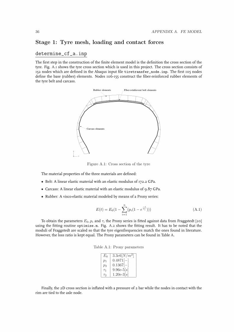
determine_cf_a.inpThe first step in the construction of the finite element model is the definition the cross section of thetyre. Fig. A.1 shows the tyre cross section which is used in this project. The cross section consists of152 nodes which are defined in the Abaqus input file tiretransfer_node.inp. The first 105 nodesdefine the base (rubber) elements. Nodes 106-155 construct the fiber-reinforced rubber elements ofthe tyre belt and carcass.

X

YZ

Fiber-reinforcent belt elementsRubber elements

Carcass elements

Figure A.1: Cross section of the tyre

The material properties of the three materials are defined:

• Belt: A linear elastic material with an elastic modulus of 172.2 GPa.

• Carcass: A linear elastic material with an elastic modulus of 9.87 GPa.

• Rubber: A visco-elastic material modeled by means of a Prony series:

E(t) = E0(1−n∑

i=1

(pi(1− e−tτi ))) (A.1)

To obtain the parameters E0, pi and τi the Prony series is fitted against data from Fraggstedt [20]using the fitting routine optimize.m. Fig. A.2 shows the fitting result. It has to be noted that themoduli of Fraggstedt are scaled so that the tyre eigenfrequencies match the ones found in literature.However, the loss ratio is kept equal. The Prony parameters can be found in Table A.

Table A.1: Prony parameters

E0 3.3e6[N/m2]p1 0.4871[−]p2 0.1367[−]τ1 9.96e-5[s]τ2 1.20e-3[s]

Finally, the 2D cross section is inflated with a pressure of 2 bar while the nodes in contact with therim are tied to the axle node.

37

10-2

100

102

104

106

1

1.5

2

2.5

3

3.5x 10

6 Storage modulus

Frequency [Hz]

Re(

E)

[Pa]

FraggstedtFit

(a)

10-2

100

102

104

106

0

1

2

3

4

5

6

7

8

9x 10

5 Loss modulus

Frequency [Hz]

Im(E

) [P

a]

FraggstedtFit

(b)

10-2

100

102

104

106

0

0.05

0.1

0.15

0.2

0.25

0.3

0.35

0.4Tan(δ)

Frequency [Hz]

Los

s ra

tio

[-]

FraggstedtFit

(c)

Figure A.2: Prony series material model in the frequency domain (a) Storage modulus (b) Lossmodulus (c) Lossfactor.


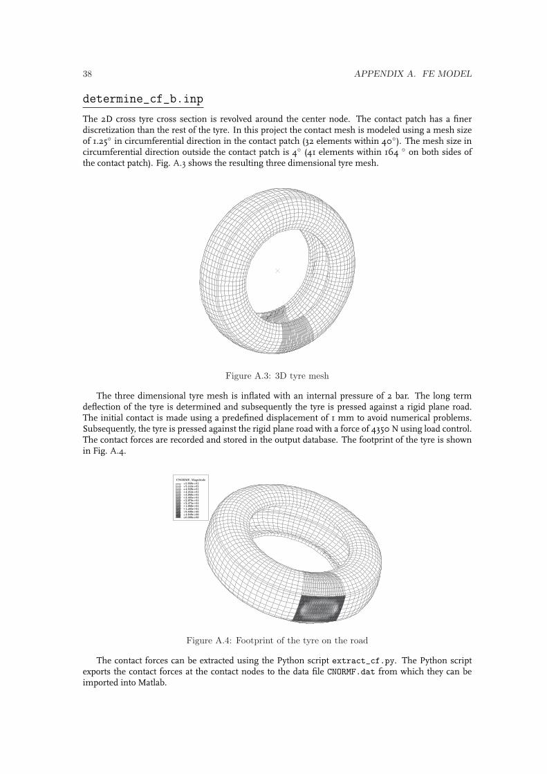
determine_cf_b.inpThe 2D cross tyre cross section is revolved around the center node. The contact patch has a finerdiscretization than the rest of the tyre. In this project the contact mesh is modeled using a mesh sizeof 1.25 in circumferential direction in the contact patch (32 elements within 40). The mesh size incircumferential direction outside the contact patch is 4 (41 elements within 164 on both sides ofthe contact patch). Fig. A.3 shows the resulting three dimensional tyre mesh.

Figure A.3: 3D tyre mesh

The three dimensional tyre mesh is inflated with an internal pressure of 2 bar. The long termdeflection of the tyre is determined and subsequently the tyre is pressed against a rigid plane road.The initial contact is made using a predefined displacement of 1 mm to avoid numerical problems.Subsequently, the tyre is pressed against the rigid plane road with a force of 4350 N using load control.The contact forces are recorded and stored in the output database. The footprint of the tyre is shownin Fig. A.4.

CNORMF, Magnitude

+0.000e+00+4.949e+00+9.899e+00+1.485e+01+1.980e+01+2.475e+01+2.970e+01+3.465e+01+3.960e+01+4.454e+01+4.949e+01+5.444e+01+5.939e+01

Figure A.4: Footprint of the tyre on the road

The contact forces can be extracted using the Python script extract_cf.py. The Python scriptexports the contact forces at the contact nodes to the data file CNORMF.dat from which they can beimported into Matlab.

39

Stage 2: Steady state rolling analysis

SST_axleforce.inpFirst, the tyre mesh is constructed from the start using the results from determine_cf_a. The tyre isloaded as described in the previous section only now a load of 4100 N is applied. Friction of the roadis set to zero. The steady state rolling analysis is performed at a velocity of 80 km/h which, at a tyreradius of 316 mm, corresponds to an angular velocity of 70.2 rad/s. The tyre stiffens during rotation.Therefore, the position of the tyre with respect to the road is load controlled. The total reaction forceshould therefore remain at 4100 N and is exported to the database for verification. Furthermore, theresisting moment around the central rim node is exported to the database to determine the energydissipation in the tyre.

In the steady state rolling analysis a zero friction between the road and the tyre is assumed. Inreality this is obviously not the case as the tyre would not create any traction. This analysis thereforedoes not simulate a free-rolling tyre: the resisting forces are not equal to the traction forces. However,in the current analysis the focus lies on rolling resistance forces instead of traction forces. The as-sumption is that with friction the contact patch has approximately the same shape as without friction.Therefore, the rolling resistance is assumed to be the same in both cases.

The total contact force and the resisting moment around the central rim node can be importedinto Matlab using the Python script extract_RRmoment.py. The Python script extracts the forces andmoments to a data file moment.dat from which they can be imported into Matlab.

The energy dissipation RRSSTpower can be determined by:

RRSSTpower =RRSSTmomentv

rtyre(A.2)

in which v represents the velocity and rtyre represents the tyre radius. The rolling resistancecoefficient RRSSTrrc can be determined by:

RRSSTrrc =RRSSTpower

Naxlev(A.3)

in which Naxle represents the axle load.


Stage 3: Modal analysis

Ab_ex_tire_1.inpThe tyre is constructed constructed again from scratch. The only difference is the definition of thematerial parameters. During a modal analysis the visco-elastic material must be evaluated at a prede-fined frequency. Therefore, the visco-elastic material properties are replaced by a linear elastic materialmodel. The elasticity is chosen to be equal to 1.4 MPa which is the storage modulus in the visco-elasticmaterial at a frequency of 100 Hz.

Furthermore, a new node set is defined which contains the master nodes. The master nodes willbe retained in subsequent model reduction techniques. The master nodes can be divided into twocategories. The boundary master degrees of freedom (6 nodes) are used to fix the tyre to the rim. Theinternal master degrees of freedom give a reduced representation of the tyre. The master nodes areillustrated in Fig. A.5.

X

YZ

Internal master degrees of freedom

Boundary master degrees of freedom

Figure A.5: Masternodes in a cross section of the tyre

make_modal_analysis.mThe rim nodes are untied to the axle node. The recorded contact forces from the first section areapplied to the contact nodes. These forces are therefore written to the Abaqus input file using the theMatlab script make_modal_analysis.m. This script adapts the Abaqus file modal_analysis.inp sothat it contains the appropriate contact forces from the data file CNORMF.dat.

41

modal_analysis.mIn the modal analysis the first 600 eigenfrequencies and eigenmodes are determined and writtento the output database. Fig. A.6 shows one such eigen mode at a frequency of 129 Hz. Addition-ally, the reduced mass matrix which only contains the master nodes is exported to the output filemodal_analysis.fil.

Figure A.6: Eigenmode of the tyre at 129 Hz.

The output file can be imported using the Matlab script ab2mat.m. It has to be noted that thisis a process which requires a lot of computational effort. ab2mat.m outputs the structure model thatcontains the base coordinates of the mesh, the mass matrix, eigenmodes and eigenfrequencies. Thisstructure is saved as a Matlab file system_matrices.mat for further use.

Appendix B

Tyre/road interaction model

This chapter provides a detailed description of the tyre/road interaction model. First, the global struc-ture of the model is discussed and then the individual Matlab functions will be discussed in detail.

A graphical overview of the numerical model with the different functions is given in Fig. B.1. Thebasis of the code is the file start_up.m which runs the entire analysis. The complete analysis can bedivided into three stages which will be discussed separately.:

1. The first stage is the modal transformation of the system matrices and the construction of theGreen’s functions.

2. The second stage is the tyre/road interaction model.

3. The third stage consists of postprocessing and visualization of the results.

During these stages the results and variables will be stored in different structures as shown inTable B.1

Table B.1: Road structure categories

Matlab structure Content

var Input and dependent variablesmodel System matrices and coordinatesmodtrans Matrices used in the modal transformationgreen Green’s functions and time vectorroad Raw and discretized road datasimu Tyre/road interaction simulation resultsanim Animation dataresults Results from the rolling resistance analysis

Before the first stage starts in the function start_up.m, the data from the FEM analysis is loadedinto Matlab:

• Mass matrix, eigen modes and eigen frequencies in model

• Node coordinates and indices in model

• Road data in road

• Contact forces in contact

43

44 APPENDIX B. TYRE/ROAD INTERACTION MODEL

Start up.m_

Load modes 3d.m_ _

Modal transform.m_

Spat der ruudnonuni cond.m

_ _ _

_

Rotate modes2.m_

Green func analytic.m_ _

Contact nodes.m_

Solve contact problem.m

_ _

Road texture.m_

Contact problem.m_ Nonlinearspring.m

Springdamper.m

Rolling_resistance.m

Animate_patch.m

Animate_tyre.m

Tyre_deformation.m

Lsqnonlin.m

1. Modal transformation and Green s functions’

3. Postprocessing

2. Tyre/road interaction modeling

Input variables.m_

Timestep.m

Green eval.m_

Figure B.1: File structure of the tyre/road interaction model

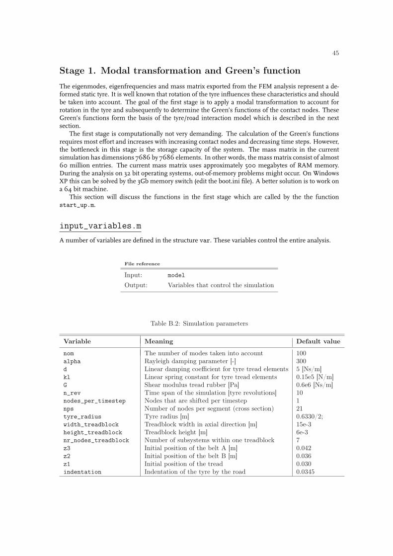
45

Stage 1. Modal transformation and Green’s function

The eigenmodes, eigenfrequencies and mass matrix exported from the FEM analysis represent a de-formed static tyre. It is well known that rotation of the tyre influences these characteristics and shouldbe taken into account. The goal of the first stage is to apply a modal transformation to account forrotation in the tyre and subsequently to determine the Green’s functions of the contact nodes. TheseGreen’s functions form the basis of the tyre/road interaction model which is described in the nextsection.

The first stage is computationally not very demanding. The calculation of the Green’s functionsrequires most effort and increases with increasing contact nodes and decreasing time steps. However,the bottleneck in this stage is the storage capacity of the system. The mass matrix in the currentsimulation has dimensions 7686 by 7686 elements. In other words, the mass matrix consist of almost60 million entries. The current mass matrix uses approximately 500 megabytes of RAM memory.During the analysis on 32 bit operating systems, out-of-memory problems might occur. On WindowsXP this can be solved by the 3Gb memory switch (edit the boot.ini file). A better solution is to work ona 64 bit machine.

This section will discuss the functions in the first stage which are called by the the functionstart_up.m.

input_variables.mA number of variables are defined in the structure var. These variables control the entire analysis.

File reference

Input: model

Output: Variables that control the simulation

Table B.2: Simulation parameters

Variable Meaning Default value

nom The number of modes taken into account 100alpha Rayleigh damping parameter [-] 300d Linear damping coefficient for tyre tread elements 5 [Ns/m]kl Linear spring constant for tyre tread elements 0.15e5 [N/m]G Shear modulus tread rubber [Pa] 0.6e6 [Ns/m]n_rev Time span of the simulation [tyre revolutions] 10nodes_per_timestep Nodes that are shifted per timestep 1nps Number of nodes per segment (cross section) 21tyre_radius Tyre radius [m] 0.6330/2;width_treadblock Treadblock width in axial direction [m] 15e-3height_treadblock Treadblock height [m] 6e-3nr_nodes_treadblock Number of subsystems within one treadblock 7z3 Initial position of the belt A [m] 0.042z2 Initial position of the belt B [m] 0.036z1 Initial position of the tread 0.030indentation Indentation of the tyre by the road 0.0345


contact_nodes.mThe contact patch can vary in size with respect to time. Therefore, the nodes are determined whichpotentially make contact with the road. This is done in the function contact_nodes.m.

File reference

Input: model,contact

Output: Potential contact nodesContact node indices

• First, the structure model.base_co is adjusted so it contains the coordinates of the reduced setof tyre nodes instead of all nodes. Then the structure model.def_coord is created so that isconsists the deformed coordinates of the subset of tyre nodes.

• In Abaqus an axle load of 4350 N was applied to the tyre. However, the desired axle load isonly 4100 N. Therefore, all the nodes that potentially make contact with the road are alreadyidentified. The node numbers and forces are stored in the structure contact.force. Theposition of these nodes in the coordinate matrix model.base_co is determined and stored inthe vector contact.node_indices_all_vec

• The rows on which the contact nodes are located are identified. These rows are illustrated inFig. B.2 and stored in the vector contact.node_row.

• Every node has three coordinates. The position of the first coordinate of each node in the eigen-mode matrix is determined. Finally the contact forces are conveniently stored in the vectorF_init.

22055 22555 23055 23555 24055 24555 25055

22605 23105 23605 24105 24605

22550 23050 23550 24050 24550

23100 23600 24100

23045 23545 24045

Contact node row 7 6 5 4 3 2 1

Figure B.2: Simplified illustration of the contact patch, node numbers and contact rows

47

timestep.mThe frequency is determined at which the Green’s function are sampled. This depends on the length ofan element in circumferential direction, the vehicle velocity and the number of nodes that are shiftedper time step.

File reference

Input: model,var,contact

Output: Time stepLength of a contact patch element in circumferential direction

• First, the length of an element is determined by taking the difference between the maximumand minimum of the x coordinate in model.def_coord and dividing this by the number ofcontact rows.

• The time step is defined as the length of an element divided by the vehicle velocity.

• The length of a treadblock is determined as the amount of nodes per treadblock times the lengthof an element.

load_modes3D.mThe eigen modes and eigen frequencies are loaded.

File reference

Input: model,var

Output: Base coordinates of the nodes modtrans.base_co_fullMatrix with eigenvectors modtrans.USparse matrix of eigenfrequencies modtrans.V

• The base coordinates are stored in a new vector modtrans.base_co_full and the eigenmodesare stored in a new matrix modetrans.U. This matrix has the dimension 3*var.non timevar.nom:

base co full =_ _

x1

y1

z1

x2

y2

z2

x3

y3

z3

U =

x1

y1

z1

x2

y2

z2

x3

y3

z3

x1

y1

z1

x2

y2

z2

x3

y3

z3

x1

y1

z1

x2

y2

z2

x3

y3

z3

Mode 1

Mode 2

Mode 3

Mode i

• The eigen frequencies are stored in a sparse matrix var.V


modal_transform.mThe modal transformation is applied to the system matrices.

File reference

Input: model,modtrans,var

Output: Matrix of right and left eigenvectors modtrans.U_1 and modtrans.U_2Vector with (left) eigen frequencies modtrans.s_1The (near diagonal) matrix modtrans.a

• First, the Rayleigh damping matrix D is defined with the Rayleigh variable var.alpha

• Next the system matrices are modified to account for the rotation of the tyre. The time derivativesof the eigenmodes are determines in rotate_modes2.m. Therefore, the spatial derivatives of theeigenmodes have to be determined by spat_der_nonuni_cond_ruud.m. For further referenceon the transformation the reader is referred to [26, 25, 28, 27].

• The system is rewritten in a first order form. Subsequently, the matrix of right and left eigen-vectors modtrans.U_1 and modtrans.U_2 is constructed, the vector with eigen frequenciesmodtrans.s_1 is constructed and the (near diagonal) matrix modtrans.a is determined.

green_func_analytic.m

The Green’s function are precalculated.

File reference

Input: modtrans,contact,var

Output: Matrix (size: non*non*time_samples) with green’s function green.functionsTime samples for Green’s functionsMatrix with green’s function shifted 1 dimension green.functions_shiftdim

• First, the time is defined in green.time. In the default case 200 time samples are chosen.However, is the damping is decreased or increased this should be changed. The amount of timesamples has to be sufficient for the Green’s functions to fully attenuate to zero. Too many timesamples will decrease the efficiency of the model.

• The Green’s function are constructed in green.functions using the eigenmodes of the originalsystem modtrans.U, the right and left eigenvalues of the first order system modtrans.U_1 andmodtrans.U_2, the eigenfrequencies of the first order system modtrans.s_1 and the diagonalentries of the matrix modtrans.a. Again, for further reference on the construction of theseGreen’s functions the reader is referred to [26, 28].

• The Green’s function are modified for increased efficiency during the tyre/road interaction sim-ulation. First, the beginning zero entry of the Green’s functions is deleted. This zero entrywould prevent a force in a time step to have any effect on the deformation in the same time step.This approach is in accordance to Kropp and Andersson. [36].

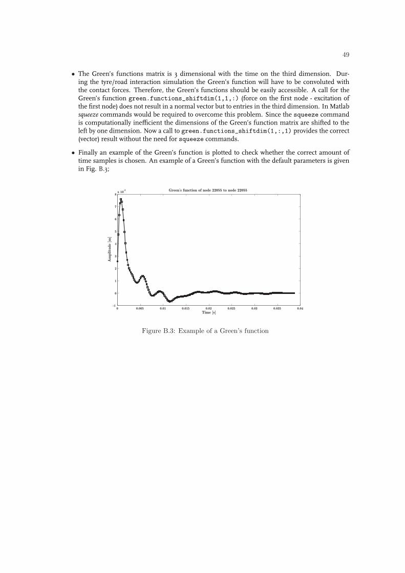
49

• The Green’s functions matrix is 3 dimensional with the time on the third dimension. Dur-ing the tyre/road interaction simulation the Green’s function will have to be convoluted withthe contact forces. Therefore, the Green’s functions should be easily accessible. A call for theGreen’s function green.functions_shiftdim(1,1,:) (force on the first node - excitation ofthe first node) does not result in a normal vector but to entries in the third dimension. In Matlabsqueeze commands would be required to overcome this problem. Since the squeeze commandis computationally inefficient the dimensions of the Green’s function matrix are shifted to theleft by one dimension. Now a call to green.functions_shiftdim(1,:,1) provides the correct(vector) result without the need for squeeze commands.

• Finally an example of the Green’s function is plotted to check whether the correct amount oftime samples is chosen. An example of a Green’s function with the default parameters is givenin Fig. B.3;

0 0.005 0.01 0.015 0.02 0.025 0.03 0.035 0.04-1

0

1

2

3

4

5

6

7

8x 10

-3

Time [s]

Am

plitu

de

[m]

Green s function of node 22055 to node 22055’

Figure B.3: Example of a Green’s function


Stage 2: Tyre/road interaction

The second stage of the analysis covers the interaction between the road surface and the tyre. In thissection a global overview of the model is provided. Subsequently, the different parts of the simulationwill be discussed in more detail. The tyre/road interaction model can be executed with the functionsolve_contact_problem.m.

Fig. B.4 provides an overview of the tyre/road contact model.

x (t)2

x (t)1

p(t)

z1

z2

f(p-z -x )1 1

kld

Green sfunctions

’

Finit

x (t)3

z3

Figure B.4: Graphical representation of the contact model

Fig. B.5 shows the algorithm which is used to solve the contact problem. Important to note isthat the forces and displacements in this diagram all represent vectors with the size of the number ofcontact nodes.

1. The algorithm starts at time N with an initial guess of the displacement at the surface of thetread block x1.

2. Using the displacement x1, the rest rest position z1, the road profile p(t) and the correspondingnonlinear stiffness function f(p − z1 − x1), the force in the nonlinear contact spring can bedetermined by the function nonlinearsping.m.

3. Using the obtained force F and the displacement from the previous time step x1,old and x2,old

the displacement of the upper side of the treadblock can be determined by springdamper.m.

4. By subtracting the initial force Finit from the force F the force on the belt is determined. Note:since the forces applied to the tyre in Abaqus were larger than required the outcome is a negativeforce pulling the belt down. Using the force and the position of the belt in the previous timestep, the position of the belt in the current time step can be determined by green.m.

5. Adding the rest position and subtracting the result from (3) and (4) results in an error whichshould be minimized. Therefore, the nonlinear least square solver lsqnonlin.m of Matlab isused. The optimization routine squares and sums the error.

6. The Matlab optimization routine updates the position x1 and iterates until the error is mini-mized and the problem has converged.

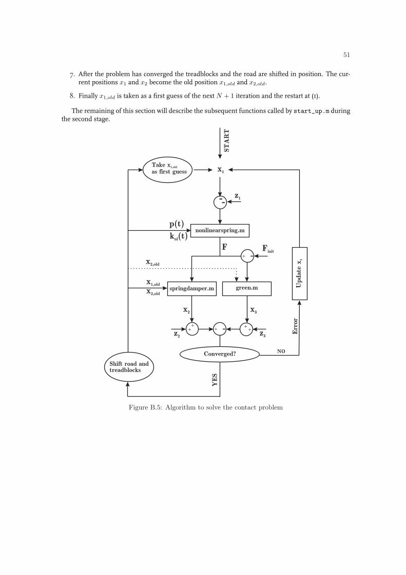
51

7. After the problem has converged the treadblocks and the road are shifted in position. The cur-rent positions x1 and x2 become the old position x1,old and x2,old.

8. Finally x1,old is taken as a first guess of the next N + 1 iteration and the restart at (1).

The remaining of this section will describe the subsequent functions called by start_up.m duringthe second stage.

x1

F

Updat

e x

1

x3x2

+ - Err

or

nonlinearspring.m

springdamper.m green.m

+ -Finit

++

z2

++

z3

Converged? NO

YES

2,oldxx1,old

p(t)

k (t)nl

Shift road andtreadblocks

Take xas first guess

1,old

ST

AR

T

-- z1

x2,old

Figure B.5: Algorithm to solve the contact problem


road_texture.mFirst, the road is divided into road sections with the length of one element. Next, the contact stiffnessof the road sections is determined.

File reference

Input: var,road

Output: Discretized profile height of road sections road.profile_road_disc_repmatContact stiffness related to the road sections road.profile_road_disc

• The resolution of the data initialized. With the data measured by M+P this is 0.2 mm.

• One road texture line is extracted from the data. In future version multiple line could be takeninto account. However, the model currently uses a 2D extruded texture profile.

• The rounded number of texture points within one element is determined as the element sizedivided by the data resolution. With the default simulation parameters there are 22 points withinone element.

• Next, the road elements are processed. The midpoint of a road section is determined and themaximum of 22 points is determined.

• The points within one section are stored and the minimum and maximum is determined. Next,an indentation array d_vec is constructed which runs from zero indentation to half indentationand consists of 100 points. Half indentation has shown to produce sufficient forces.

• The force for every indentation is determined using the function [37]:

F =3πµr4

eqdvec

2h(d)3(B.1)

in which req is the radius of a circle with the same surface area as a contact element. The heighth(d) is the un-indented part of the tread block.

• An exponential function is fitted through the contact force points. Monotonicity is crucial forthe fitted function as non-monotonic function will cause convergence problems in the solutionalgorithm. A fifth order fit in the form Ffit = a ∗ d5

vec is used which is always monotonicallyincreasing if a is positive.

• A few examples of the fitted function are plotted for a visual verification of the fit.

• One data line consists of 2.8 meters of road texture data. In one rotation the tyre already travelsmore than two meters. Therefore, to allow for multiple tyre rotation, the texture and contact stiff-ness data is copied multiple times and stored in road.profile_road_disc and road.contact_stiffness.

53

solve_contact_problem.mIn every time step the contact problem is solved. The results are stored, the tyre is rotated and a newtime step begins.

File reference

Input: var,contact,road,green,simu

Output: Displacement of the tyre belt and tread in simu.x1_store and simu.x2_storeContact forces in simu.F.

• First, the options for the optimization routine lsqnonlin are defined. In the default case theDisplay parameter is set to Iter so that the iteration progress can be monitored.

• The output matrices are filled with zero entries to decrease the computational effort.

• In the beginning of a time step, the road profile and the contact stiffness are defined for eachelement depending on the contact row of the element.

• The excitation of the belt by previously determined forces is determined by the function green.m.In the first step these forces equal zero and therefore also excitation equals zero.

• Next, the actual contact problem is solved by the Matlab optimization function lsqnonlin whichcalls the function contact_problem.m. After convergence this results in the vector of displace-ments x1_new

• From the vector x1_new all the displacement and forces in the current time step are determinedand stored.

• After each tyre rotation, the sum of the contact forces is compared to the desired load var.axle_load. If needed, the indentation of the road surface is adjusted.

• The position of the tread elements are shifted. First, the node is identified from which anothernode has to inherit its displacements (from_which). To identify these neighboring nodes the in-crementation between nodes numbers in circumferential direction is used (+500). Some nodeswill not be able to inherit displacements from other nodes because they are on the trailing edgeof the contact patch. These notes therefore inherit a zero displacement.


green.mThe displacement of the belt due to forces in previous time steps is determined. The contact forcesand Green’s function are convoluted.

File reference

Input: simu, contact, green, var

Output: Displacement of the tyre belt due to forces in previous time steps.

• The force at a contact node k is convoluted with the Green’s function of all the contact nodesaccording to:

xB2 (N) ∼= F (N)g(1)∆t +

N−1∑n=1

F (n)g(N − n + 1)∆t (B.2)

• The resulting displacements for all forces are summed to determine the overall displacementsimu.x3_greenold.

contact_problem.mThe error is calculated between the displacement of the belt determined by the Green’s function x2and the displacement of the belt determined by the spring-damper system x3 .

File reference

Input: x1,simu.x3_greenold,simu.x_old,var,simu,contact,green

Output: The vector of errors between x2 and x3

• Given a displacement x1, the force F in the nonlinear spring is determined by nonlinearsptring.m.

• The additional force F_add is determined with respect to the static force F_init.

• The displacement of the belt is determined resulting from additional belt forces in the currenttime step according to:

x3 = Fadd(N)g(1)∆t (B.3)

• The displacement of the belt is determined due to the force in the spring damper system by thefunction springdamper.

• The error between x2 and x3 is determined

55

nonlinearspring.mThe force generated by the nonlinear spring is determined given a displacement x1 and a nonlinearstiffness parameter simu.nlstiffness.

File reference

Input: x1,var,simu

Output: The force in the nonlinear spring F

• The indentation of the road surface d is determined.

• The force in the nonlinear spring F is calculated and divided by the number of nodes withinone tread block. The nonlinear stiffness approximation only holds for complete treadblocks.However, in this project the treadblocks are divided into multiple elements. Therefore, the forceis divided by the number of nodes per treadblock. This is a very rough estimation which needsimprovement in future versions of the model.

springdamper.mGiven the force generated by the nonlinear spring, the displacement due to deformation of the springdamper system x2 is determined .

File reference

Input: F,x1,x_old,var.kl,var.d,var.delta_t

Output: The displacement of the belt x2

• The displacement of the belt is approximated according to

xA2 (N) ∼= d(x1(N)− x1(N − 1))− F (N)δt + dx2(N − 1) + δtklx1(N)

d + δtkl(B.4)


Stage 3: Postprocessing

In the third stage of the simulation the rolling resistance is determined, the vibrations in the completetyre are calculated and finally the simulation outcomes are visualized. Calculating the complete vibra-tions is a computationally intensive process. The Green’s functions of all nodes have to be determinedand convoluted with the recorded contact forces. Therefore, visualization of the complete tyre shouldonly be performed for presentational purposes. Instead, the contact patch visualization can be usedwhich is much faster. This section will discuss the subsequent functions called in the third stage.

rolling_resistance.mGiven the displacement of the belt and the contact forces the rolling resistance is determined. Thetimeframe in which the rolling resistance is calculated is very important. When the beginning state ofx1 is different from the end state there is a difference in potential energy between the states which isnot lost but can be recovered. Hence, rolling resistance will not be approximated correctly.

File reference

Input: simu,var,from_index,nr_rev

Output: The energy dissipation during nr_rev revolution results.E_dissipationThe power dissipation results.rollingresistance_wattsThe rolling resistance coefficient results.rollingresistance_coefficient

• The end time is defined between n_rev and n_rev+1 revolutions after from_index.

• The end time is chosen such that the difference between the beginning and end state is minimal.

• The dissipated energy is determined according to

Edis =∫ t2

t1

F i(t)xi1(t)dt (B.5)

• The power dissipation is determined by dividing by the time frame and the rolling resistance iscalculated by

RRC =Pdis

Naxlev(B.6)

57

tyre_deformation.mTo analyze the vibrations of the complete tyre, the contact forces have to be convoluted with the Green’sfunctions. Therefore, the Green’s functions of all the tyre nodes have to determined. The Green’sfunctions matrix determined earlier in the analysis (173 by 173 by 200) only covers the contact nodesand is approximately 50 Mb in size. The Green’s function matrix of the complete tyre (7686 by 7686by 200) would therefore approximately equal 100 Gb in data. Obviously, such a file can not be handledproperly and therefore the Green’s function are determined one by one and immediately convolutedwith the appropriate contact forces.

File reference

Input: modtrans,sim,var

Output: The deformation of the tyre nodes at each time step in deformation

• Initialize the Green’s functions matrix which is two dimensional: the number of nodes timenumber time samples in the Green’s function

• The force on every node j is treated separately analogue to green_func_analytic.m.

• For every time step N, the contact forces on node j are convoluted with all the Green’s functionat all the time steps and stored in deformation(N,:).

animate_patch.m and animate_tyre.mBy visualization of the contact patch a quick visual inspection of the simulation result can be per-formed. There is no need to recalculate the tyre deformation and therefore little computational effortis required.

File reference

Input: simu,contact,model,road,var

Output: Animation (avi) file of the contact patch

• A movie object is created which is encoded by a Cinepak codec which can be played on mostcomputers without additional software. Note: When errors occur in animate_patch the movieobject is not closed and errors will occur if not closed properly before proceeding.

• The displacement in the tread elements with a zero contact stiffness is increased so that treadblocks are visible.

• Every time step the figure is updated and the frame is captured and added to the movie file.

Appendix C

Regression Analysis

59

M+P – consulting engineers

Müller-BBM group

noise - vibrations - air quality

Wolfskamerweg 47, Vught

P.O. Box 2094

5260 CB Vught

The Netherlands

T +31 (0)73-658 9050

F +31 (0)73-658 9051

[email protected]

www.mp.nl

Final report

Influence of Road Surface Properties on Rolling Resistance of Car

Tyres

Prepared for Report No. Authors

M+P.DVS.08.17.1

Revision

1 S.W. Boere

Date

23 January 2008 Dr. G.J. van Blokland

Dienst Verkeer en

Scheepvaart

Postbus 5044

2600 GA DELFT

Order No. Page

Bestelnummer: 4500133762 60 of 45

© M+P – consulting engineers

No part of this publication may be used for purposes other than agreed upon by client

and M+P (DNR 2005 Art. 46).

Offices in Aalsmeer and Vught

Member of ONRI ISO 9001

M+P.DVS.08.17.1,

61

Summary

Rolling resistance is one of the main factors concerning vehicle energy consumption. Together with

aerodynamic resistance, inertial forces and climbing forces it constitutes to the total force a vehicle

has to overcome to maintain constant speed. The relative importance of rolling resistance

compared to the other factors varies with the vehicle velocity and driving pattern. On a level road

with constant speed (60 – 120 km/h) the relative importance varies from 60-38% respectively. On

uneven roads with uneven driving patterns the averaged relative fuel consumption due to rolling

resistance is approximately 14%. Lowering rolling resistance forces can therefore contribute to

energy efficient transportation. It is often estimated that lowering the rolling resistance by 10% could

give a reduction in fuel consumption of 2-3 %.

This project focuses on the influence of road surface properties on rolling resistance. Additionally,

possible conflicting requirements concerning tyre/road noise and skid resistance are examined.

Measurements on rolling resistance, texture, mechanical impedance, skid resistance and noise

were carried out on a test track with 41 different road surfaces in Kloosterzande. Amongst those

surfaces is a number of unconventional noise reducing surfaces. The rolling resistance

measurements were carried out with a specially designed trailer from the University of Gdansk

(Poland).

The observed rolling resistance coefficients are comparable to the ones found in literature. Outliers

come from rarely used and very rough surface dressings and unconventional flexible surfaces.

Some measurements appear to have a large spread which poses questions on the accuracy of the

results.

Strong correlations between texture spectra levels and rolling resistance are found in both macro

(wavelengths 0.5-50 mm) and mega (50 – 500 mm) texture regions. However, there appears to be

a strong inter-correlation between these texture regions and therefore the independent relative

influence remains unclear. Literature sources even suggest a stronger influence from shortwave

unevenness (wavelengths 0.5 – 5m) although these sources include suspension losses

Texture amplitude characteristics appear to have a good correlation with rolling resistance. Varying

Rms texture levels for conventional surfaces by 50% can have a reduction of the rolling resistance

of 7-10%. Outliers in this correlation are caused by rarely used surface dressings and flexible

rubber surfaces. The off-trend behavior of the surface dressing can probably be related to the non-

skew texture profiles.

For the flexible rubber surfaces the mechanical impedance is measured by excitation of the surface

using a shaker. A simple dynamic system is proposed to model the surface dynamics containing a

characteristic rubber mass. The acquired frequency response functions are reproducible and give

valuable information on the dynamic behavior of the surface. The real part of the admittance (the

inverse of the impedance) provides a measure of the frequency dependent energy dissipation. The

relevant frequency range is estimated to be 250-400 Hz. In this range, higher energy dissipation

corresponds with higher rolling resistance. Further research is required to determine the relevant

frequency range and to study the velocity dependency of the results. However, measuring

mechanical impedance seems to be a promising method for the analysis and optimization of flexible

road surfaces.

M+P.DVS.08.17.1,

62

No conflicting requirements were found between skid resistance and rolling resistance. Skid

resistance is assumed to depend on micro texture levels (wavelengths <0.5mm). Rolling resistance

however depends on larger wavelengths. Further research is required to study the correlation

between wet skid resistance and rolling resistance.

No clear correlation can be found between rolling resistance and tyre/road noise. However,

amongst surfaces that share the same structure, a higher Rms texture depth will result in a higher

tyre/road noise level. Therefore, no conflicting requirements are found between lowering rolling

resistance and decreasing tyre/road noise.

M+P.DVS.08.17.1,

63

Contents

Summary 61

1 Introduction 64 1.1 Literature Review 64 1.2 Objectives 66

2 Rolling resistance 67 2.1 Background 67 2.2 Measurement setup 68 2.3 Measurement results 70 2.4 Measurement Limitations 73

3 Road texture 74 3.1 Background 74 3.2 Measurement setup 75 3.3 Measurement results 76 3.4 Measurement limitations 78

4 Mechanical impedance 79 4.1 Background 79 4.2 Measurement setup 79 4.3 Measurement results 80 4.4 Dynamic road surface model 82

5 Skid resistance 85 5.1 Background 85 5.2 Measurement setup 85 5.3 Measurement results 85 5.4 Measurement limitations 86

6 Tyre/road noise 87 6.1 Background 87 6.2 Measurement setup 87 6.3 Measurement results 87

7 Regression analysis 89 7.1 Influence of surface texture on rolling resistance 89 7.2 Influence of mechanical impedance on rolling resistance 95 7.3 Correlation between skid resistance and rolling resistance. 97 7.4 Correlation between rolling resistance and tyre/road noise 99

8 Conclusion 100

References 101

M+P.DVS.08.17.1,

64

1 Introduction

Rolling resistance is one of the main factors concerning vehicle energy consumption. Together with

aerodynamic resistance, inertial forces and climbing forces it constitutes to the total force a vehicle

has to overcome to maintain constant speed. The relative importance of rolling resistance

compared to the other factors varies with the vehicle velocity and driving pattern. On a level road

with constant speed (60 – 120 km/h) the relative importance varies from 60-38% respectively. On

uneven roads with uneven driving patterns the averaged relative fuel consumption due to rolling

resistance is approximately 14%. Lowering rolling resistance forces can therefore greatly contribute

to energy efficient transportation. It is often estimated that lowering the rolling resistance by 10%

could give a reduction in fuel consumption of 2-3 %.

Although tyre design has a large influence on the reduction of rolling resistance, road surface

properties cannot be neglected. This study focuses on the road surface influence on rolling

resistance. For this purpose measurements are carried out on a test track located in Kloosterzande.

The Kloosterzande test track contains 41 different conventional and unconventional road surfaces

of approximately 60 meter each. The road surfaces differ in structure, material and chipping size. A

number of noise reducing surfaces containing rubber are included. These surfaces are generally

assumed to have higher rolling resistance. Numerous properties of the road surfaces, such as

macro and mega texture, unevenness, skid resistance and mechanical impedance, have already

been measured for other purposes. Appendix A lists all the road surfaces and gives a short

description. The rolling resistance measurements are carried out with a trailer designed by the

University of Gdansk (Poland).

1.1 Literature Review

There is limited information available in literature on the reduction of rolling resistance. Due to the

increased interest in the reduction of fuel consumption and CO2 emissions the topic becomes

increasingly important. The SILVIA project [1], a European Commission Program, provides an

interesting overview of the work done up till 2004.

One of the first and still very relevant attempts to study the relationship between road surface

properties and fuel consumption was carried out by the Swedish National Road and Transport

Institute (VTI) in Sweden in the 1980th [2]. Texture profile and fuel consumption were measured on

20 different surfaces with constant speed (50-70 km/h). Positive correlations were observed

between shortwave unevenness, megatexture, macrotexture and fuel consumption. However,

strong inter correlations were found between those texture regions. It is shown that larger

wavelengths have a higher influence on rolling resistance. The amount of shortwave unevenness

can have an effect up to 10% in fuel economy. However, as the driving speed increases, macro

texture levels increase in importance.

Report [3] from the VTI summarizes earlier work. Possible correlations were suggested between all

spectra bands including microtexture and rolling resistance. It is noted that rough macro texture can

have a positive effect on rolling resistance on wet roads. Furthermore, it is suggested that the

stiffness and softening behavior of road surfaces can be a significant factor in rolling resistance.

A study based on French data [4] indicates the relationship between rolling resistance and fuel

consumption. On average is shown that a doubling in rolling resistance increases the fuel economy

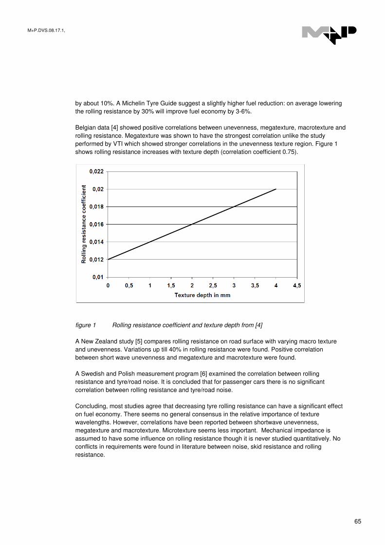
M+P.DVS.08.17.1,

65

by about 10%. A Michelin Tyre Guide suggest a slightly higher fuel reduction: on average lowering

the rolling resistance by 30% will improve fuel economy by 3-6%.

Belgian data [4] showed positive correlations between unevenness, megatexture, macrotexture and

rolling resistance. Megatexture was shown to have the strongest correlation unlike the study

performed by VTI which showed stronger correlations in the unevenness texture region. Figure 1

shows rolling resistance increases with texture depth (correlation coefficient 0.75).

figure 1 Rolling resistance coefficient and texture depth from [4]

A New Zealand study [5] compares rolling resistance on road surface with varying macro texture

and unevenness. Variations up till 40% in rolling resistance were found. Positive correlation

between short wave unevenness and megatexture and macrotexture were found.

A Swedish and Polish measurement program [6] examined the correlation between rolling

resistance and tyre/road noise. It is concluded that for passenger cars there is no significant

correlation between rolling resistance and tyre/road noise.

Concluding, most studies agree that decreasing tyre rolling resistance can have a significant effect

on fuel economy. There seems no general consensus in the relative importance of texture

wavelengths. However, correlations have been reported between shortwave unevenness,

megatexture and macrotexture. Microtexture seems less important. Mechanical impedance is

assumed to have some influence on rolling resistance though it is never studied quantitatively. No

conflicts in requirements were found in literature between noise, skid resistance and rolling

resistance.

M+P.DVS.08.17.1,

66

1.2 Objectives

The objective of this project is threefold:

- Establish a relationship between road texture and rolling resistance

- Study the correlation between mechanical impedance and rolling resistance.

- Examine the possible conflict in requirements between noise reduction and the reduction of

rolling resistance.

This report is organized as follows. First, Chapter 2 provides a theoretical background on rolling

resistance and discusses the rolling resistance measurement setup. Furthermore, the measurement

results are presented and the limitations of the measurements are discussed. Chapter 3 presents

the road texture measurements and introduces multiple measures to characterize texture. Next,

Chapter 4 introduces a method to measure the dynamic behavior of a road surface, the mechanical

impedance. Subsequently, Chapter 5 discusses the measurements on skid resistance. Chapter 6

provides a brief background on tyre/road noise and presents the measurements results using the

CPX method. Further, Chapter 7 provides an analysis of the correlations between rolling resistance,

road texture, mechanical impedance, skid resistance and tyre/road noise. Finally, Chapter 8

contains a conclusion and discussion.

M+P.DVS.08.17.1,

67

2 Rolling resistance

2.1 Background

Rolling resistance is generally defined as the energy consumed by a tyre per unit of distance

covered [9]. The main source of energy consumption is the continuous deformation of the tyre. The

rubber elements deform in the contact patch and thereby consume energy as a result of their

viscoelastic properties. This energy is not fully recovered when the elements return to the original

state. The consumed hysteresis energy is converted to heat. The amount of energy loss due to

rubber element deformation depends on the tyre geometry, tyre material properties, tyre

temperature, tyre inflation pressure and road surface properties. This project concerns the influence

of the road surface properties on the rolling resistance. Road texture is assumed to be the most

important in this sense.

Figure 2 shows a graphical representation of the mechanical manifestation of rolling resistance. The

part of the tyre which makes contact with the road is called the contact patch. The force distribution

within the contact patch as the tyre is rolling is not uniform [10]. The resultant force is located in the

front of the contact patch. This resultant force acts as a torque that opposes the wheel rotation. This

torque can also be represented by the rolling resistance force Fr which has to be overcome to

maintain constant speed.

figure 2 Graphical representation of the rolling resistance force

Rolling resistance forces linearly depend on the applied axle load in the practical range of axle

loads [10]. Consequently, a dimensionless rolling resistance coefficient, RRC, can be introduced in

which N represents the axle load and Fr represents the rolling resistance force:

(1) ][Fr

−=N

RRC

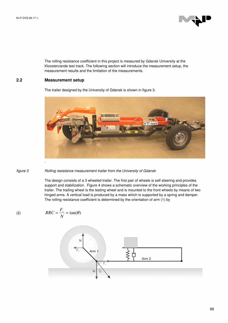
M+P.DVS.08.17.1,

68

The rolling resistance coefficient in this project is measured by Gdansk University at the

Kloosterzande test track. The following section will introduce the measurement setup, the

measurement results and the limitation of the measurements.

2.2 Measurement setup

The trailer designed by the University of Gdansk is shown in figure 3.

.

figure 3 Rolling resistance measurement trailer from the University of Gdansk

The design consists of a 3 wheeled trailer. The first pair of wheels is self steering and provides

support and stabilization. Figure 4 shows a schematic overview of the working principles of the

trailer. The trailing wheel is the testing wheel and is mounted to the front wheels by means of two

hinged arms. A vertical load is produced by a mass which is supported by a spring and damper.

The rolling resistance coefficient is determined by the orientation of arm (1) by

(2) )tan(θ==N

FRRC r

M+P.DVS.08.17.1,

69

figure 4 Schematic representation of the measurement trailer

The angle between the two arms is measured by an inductive sensor. The system is compensated

for tilt of arm (2) and for possible acceleration or road surface gradients. The advantage of this

method is that only the angle θ has to be monitored which gives a direct measure of the rolling

resistance coefficient.

The trailer is driven at a constant speed of 80 km/h over the test track. A trigger records the

transition from one road surface test section to the other. Multiple test runs in both directions are

averaged to compensate for road surface gradients. The two tyres that are used are listed in table I.

table I Two tyres used to measure the rolling resistance

Tyre Size

Continental CPC2 LI98

225/60 R16

Uniroyal Tiger Paw (SRTT) 225/60 R16 97S

M+P.DVS.08.17.1,

70

2.3 Measurement results

Figure 5 shows an example of the measurement results on one single test section. The rolling

resistance coefficient of the two tyres is plotted as a function of the distance travelled over section

1. The complete overview of the measurement results over all 41 test sections is digitally provided.

figure 5 Example of rolling resistance measurement test track 1, the white area represents the data window

The magnitude of the rolling resistance coefficient appears to be in the order of 1% which agrees

with other literature [10]. A window is applied to the raw data to account for transient effects in the

results. The gray area indicates data which is neglected in the analysis. Subsequently the

windowed data is averaged and the results are shown for both tyres in figure 6 and figure 7. The

results are ordered according to the surface category depicted in appendix AC. The vertical line on

top of each bar indicates the minimum and maximum recorded rolling resistance within the window.

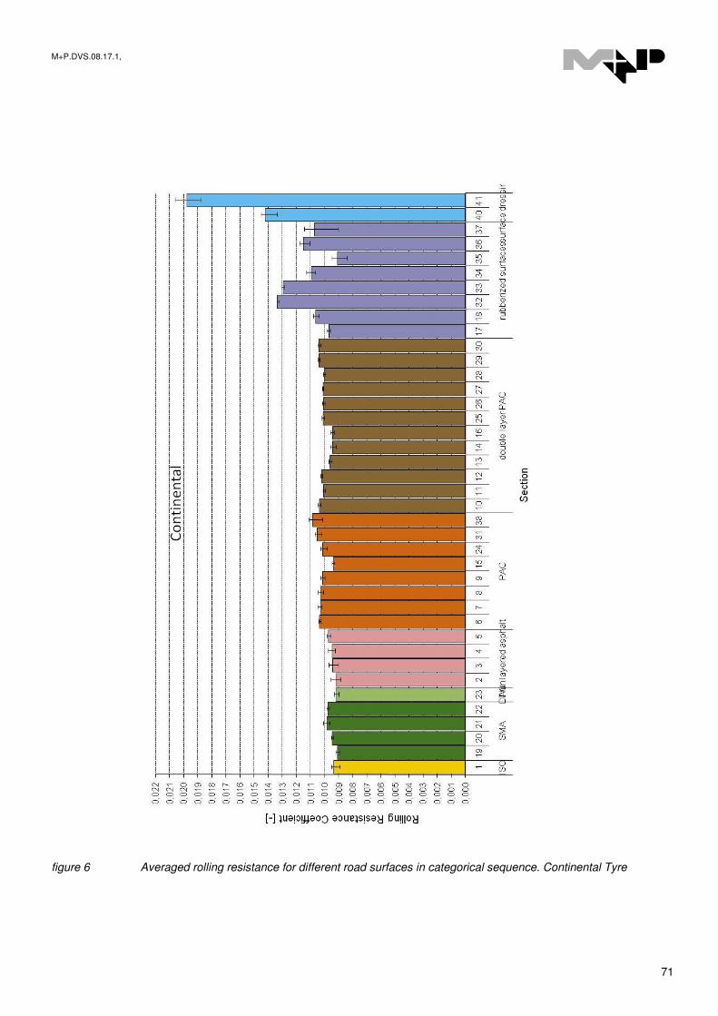
M+P.DVS.08.17.1,

71

figure 6 Averaged rolling resistance for different road surfaces in categorical sequence. Continental Tyre

M+P.DVS.08.17.1,

72

figure 7 Averaged rolling resistance for different road surfaces in categorical sequence. SRTT Tyre

M+P.DVS.08.17.1,

73

On all tested surfaces the Continental tyre appears to have a slightly higher rolling resistance (8-

15%). However, the differences between the surfaces appear to be approximately the same for

both tyres. Therefore, in further analysis only the Continental tyre data will be shown.

The results show that the variance within one category can be quite significant compared to the

differences between categories. Two surface categories, the flexible rubberized surfaces and the

surface dressings, differ greatly ins size. Interestingly, some of the rubberized surfaces perform

really well in terms of rolling resistance compared to more conventional surfaces.

2.4 Measurement Limitations

The minimum and maximum recorded rolling resistance within the measurement window gives an

indication of the reliability of the data which in some cases is quite low (surfaces 37 and 41 for

example). Therefore, one has to be careful drawing hard conclusion based on these data.

One of the main flaws of the measuring method is the length of the road sections: approximately 60

meter. At a speed of 80 km/h this corresponds to a measuring time of 2.7 seconds per section. In

some situations this time span is too short to reach a steady state situation.

Little is known about the accuracy of the trailer of the Technical University of Gdansk. The system is

compensated for accelerations and road surfaces gradients. However the system is unable to

correct both effects at the same time. Because road surface gradients are present at the

Kloosterzande test track this may increase measuring errors. Further research is required to study

the accuracy of the measuring trailer.

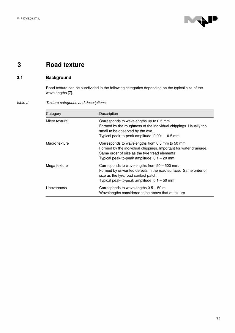
M+P.DVS.08.17.1,

74

3 Road texture

3.1 Background

Road texture can be subdivided in the following categories depending on the typical size of the

wavelengths [7].

table II Texture categories and descriptions

Category Description

Micro texture Corresponds to wavelengths up to 0.5 mm.

Formed by the roughness of the individual chippings. Usually too

small to be observed by the eye.

Typical peak-to-peak amplitude: 0.001 – 0.5 mm

Macro texture Corresponds to wavelengths from 0.5 mm to 50 mm.

Formed by the individual chippings. Important for water drainage.

Same order of size as the tyre tread elements

Typical peak-to-peak amplitude: 0.1 – 20 mm

Mega texture Corresponds to wavelengths from 50 – 500 mm.

Formed by unwanted defects in the road surface. Same order of

size as the tyre/road contact patch.

Typical peak-to-peak amplitude: 0.1 – 50 mm

Unevenness Corresponds to wavelengths 0.5 – 50 m.

Wavelengths considered to be above that of texture

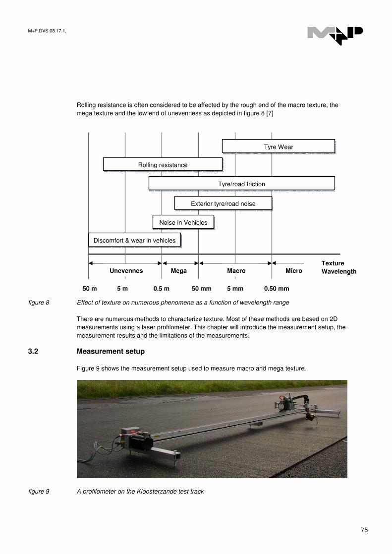
M+P.DVS.08.17.1,

75

Rolling resistance is often considered to be affected by the rough end of the macro texture, the

mega texture and the low end of unevenness as depicted in figure 8 [7]

figure 8 Effect of texture on numerous phenomena as a function of wavelength range

There are numerous methods to characterize texture. Most of these methods are based on 2D

measurements using a laser profilometer. This chapter will introduce the measurement setup, the

measurement results and the limitations of the measurements.


Figure 9 shows the measurement setup used to measure macro and mega texture.

figure 9 A profilometer on the Kloosterzande test track

Rolling resistance

Tyre Wear

Tyre/road friction

Exterior tyre/road noise

Noise in Vehicles

Discomfort & wear in vehicles

50 m

5 m 0.5 m

50 mm 5 mm

0.50 mm

Texture

Wavelength Unevennes Mega Macro Micro

M+P.DVS.08.17.1,

76

This device uses a laser interferometer which measures the height of the surface as a function of

the longitudal position. The resolution in the longitudal direction is 0.2mm. The resolution in the

lateral direction is 1 mm.


A typical output of the profilometer is shown in figure 10:

0.15 0.2 0.25 0.3 0.35

-12

-10

-8

-6

-4

-2

0

2

4

x 10-4

Distance [m]

Pro

file

heig

ht [m

m]

figure 10 A typical texture output from the profilometer

There are numerous ways to quantify texture. These include measures based on texture amplitude

and spectral analysis of the texture [11] :

- Texture wavelength spectrum

- Mean profile depth (MPD)

- Mean absolute deviation of the profile (Ra)

- Root mean square deviation of the profile (RMS)

- Skewness of the profile (Rsk)

- Kurtosis of the profile (Rku)

Texture wavelength spectrum

Using a Fourier transform the amplitude as a function of wavelength is determined. Usually the

wavelength resolution is 1/3 octave. The amplitudes are given on a logarithmic scale using a

reference value of 10-6

m.

(3) dBa

aL

ref

otx )log(20, =

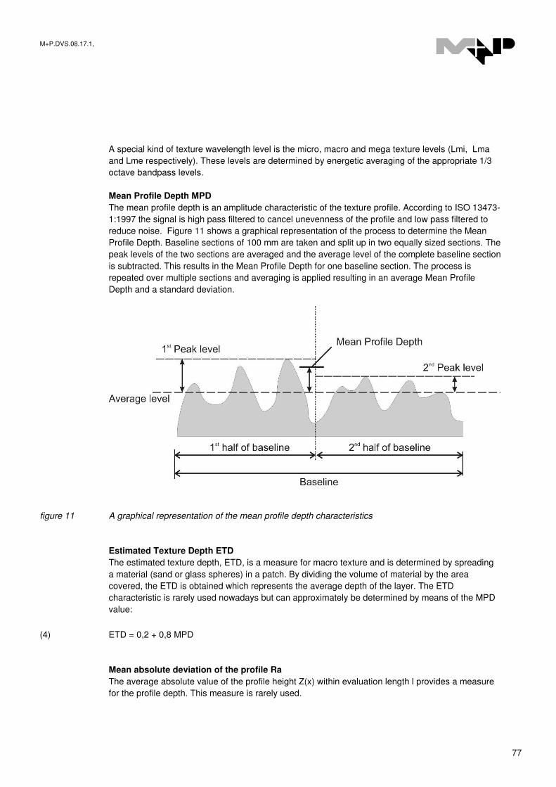
M+P.DVS.08.17.1,

77

A special kind of texture wavelength level is the micro, macro and mega texture levels (Lmi, Lma

and Lme respectively). These levels are determined by energetic averaging of the appropriate 1/3

octave bandpass levels.

Mean Profile Depth MPD

The mean profile depth is an amplitude characteristic of the texture profile. According to ISO 13473-

1:1997 the signal is high pass filtered to cancel unevenness of the profile and low pass filtered to

reduce noise. Figure 11 shows a graphical representation of the process to determine the Mean

Profile Depth. Baseline sections of 100 mm are taken and split up in two equally sized sections. The

peak levels of the two sections are averaged and the average level of the complete baseline section

is subtracted. This results in the Mean Profile Depth for one baseline section. The process is

repeated over multiple sections and averaging is applied resulting in an average Mean Profile

Depth and a standard deviation.

figure 11 A graphical representation of the mean profile depth characteristics

Estimated Texture Depth ETD

The estimated texture depth, ETD, is a measure for macro texture and is determined by spreading

a material (sand or glass spheres) in a patch. By dividing the volume of material by the area

covered, the ETD is obtained which represents the average depth of the layer. The ETD

characteristic is rarely used nowadays but can approximately be determined by means of the MPD

value:

(4) ETD = 0,2 + 0,8 MPD

Mean absolute deviation of the profile Ra

The average absolute value of the profile height Z(x) within evaluation length l provides a measure

for the profile depth. This measure is rarely used.

M+P.DVS.08.17.1,

78

(5) ∫=

l

dxxZl

Ra0

)(1

Root mean square deviation of the profile Rms

The root mean square of the profile height Z(x) within evaluation length l provides a measure for the

texture depth. This is a common measure to characterize texture.

(6) ∫=

l

dxxZl

Rms0

2)(1

Skewness of the profile Rsk

Skewness is a measure for the asymmetry of the amplitude distribution. This indicates whether the

profile curve exhibits a majority of peaks directed upwards (positive skew) or downwards (negative

skew). For a normal distribution Rsk is zero.

(7) ∫=

l

dxxZlRms

Rsk0

3

3)(

11

Kurtosis of the profile Rku:

Kurtosis refers to the weighting of the tails of a distribution and is a measure of how “flat” or “sharp”

it is in relation to a normal distribution. For example, a distribution with “long and thick tails” will

have a high Kurtosis value

(8) ∫=

l

dxxZlRms

Rku0

4

4)(

11

3.4 Measurement limitations

The profilometer is a 2D measuring device because the resolution in the lateral direction is

insufficient to obtain a full 3D texture spectrum. However, under the assumption of an isotropic

surface this might not be a problem.

The resolution of the profilometer in longitudal directions is 0.2 mm. This resolution would allow to

measure wavelengths up to 0.4 mm. The microtexture range is the wavelength region below 0.5

mm. Consequently the longitudal direction of the profilometer is insufficient for measuring micro

texture.

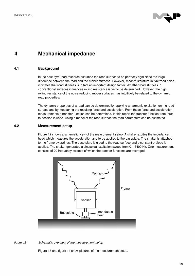
M+P.DVS.08.17.1,

79

4 Mechanical impedance

4.1 Background

In the past, tyre/road research assumed the road surface to be perfectly rigid since the large

difference between the road and the rubber stiffness. However, modern literature in tyre/road noise

indicates that road stiffness is in fact an important design factor. Whether road stiffness in

conventional surfaces influences rolling resistance is yet to be determined. However, the high

rolling resistance of the noise reducing rubber surfaces may intuitively be related to the dynamic

road properties.

The dynamic properties of a road can be determined by applying a harmonic excitation on the road

surface and by measuring the resulting force and acceleration. From these force and acceleration

measurements a transfer function can be determined. In this report the transfer function from force

to position is used. Using a model of the road surface the road parameters can be estimated.


Figure 12 shows a schematic view of the measurement setup. A shaker excites the impedance

head which measures the acceleration and force applied to the baseplate. The shaker is attached

to the frame by springs. The base plate is glued to the road surface and a constant preload is

applied. The shaker generates a sinusoidal excitation sweep from 0 – 6400 Hz. One measurement

consists of 20 frequency sweeps of which the transfer functions are averaged.

figure 12 Schematic overview of the measurement setup

Figure 13 and figure 14 show pictures of the measurement setup.

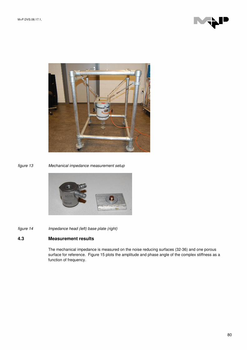
M+P.DVS.08.17.1,

80

figure 13 Mechanical impedance measurement setup

figure 14 Impedance head (left) base plate (right)


The mechanical impedance is measured on the noise reducing surfaces (32-36) and one porous

surface for reference. Figure 15 plots the amplitude and phase angle of the complex stiffness as a

function of frequency.

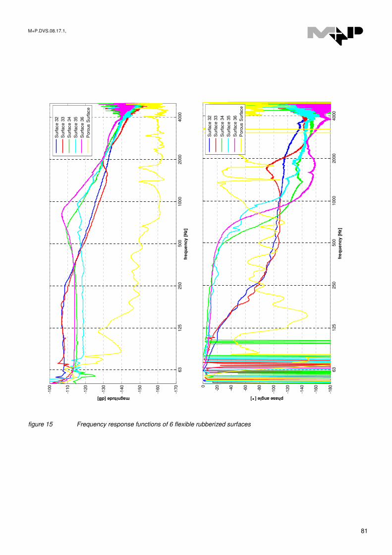
M+P.DVS.08.17.1,

81

63

125

250

500

1000

2000

4000

-170

-160

-150

-140

-130

-120

-110

-100

fre

qu

en

cy [

Hz]

magnitude [dB]

Surface 3

2

Surface 3

3

Surface 3

4

Surface 3

5

Surface 3

6

Poro

us S

urface

63

125

250

500

1000

2000

4000

-180

-160

-140

-120

-100

-80

-60

-40

-200

fre

qu

en

cy [

Hz]

phase angle [°°°°]

Surface 3

2

Surface 3

3

Surface 3

4

Surface 3

5

Surface 3

6

Poro

us S

urface

figure 15 Frequency response functions of 6 flexible rubberized surfaces

M+P.DVS.08.17.1,

82

The measurement results clearly show differences in dynamic response. The differences between

the noise reducing surfaces and the conventional porous road surface are significant.

4.4 Dynamic road surface model

The frequency response functions in figure 15 typically show one frequency peak at 125-1000 Hz

However, in some cases a second peak appears in the 1000-3000 Hz range. Therefore a two

dimensional dynamic model is introduced in figure 16. The model consists of two masses

connected to the ground and to each other by springs and dampers. The springs and dampers have

the same characteristics. In physical terms, the first mass represents the impedance head and base

plate and the second mass represents the “characteristic mass” of the rubber surface. The springs

and dampers represent the stiffness and viscoelastic behavior of the rubber.

figure 16 Road surface dynamic model

Figure 17 shows the frequency response function of surface 34 together with a model fit. In this

model fit the mass, stiffness and damping parameters are adjusted in order to match the measured

frequency response function.

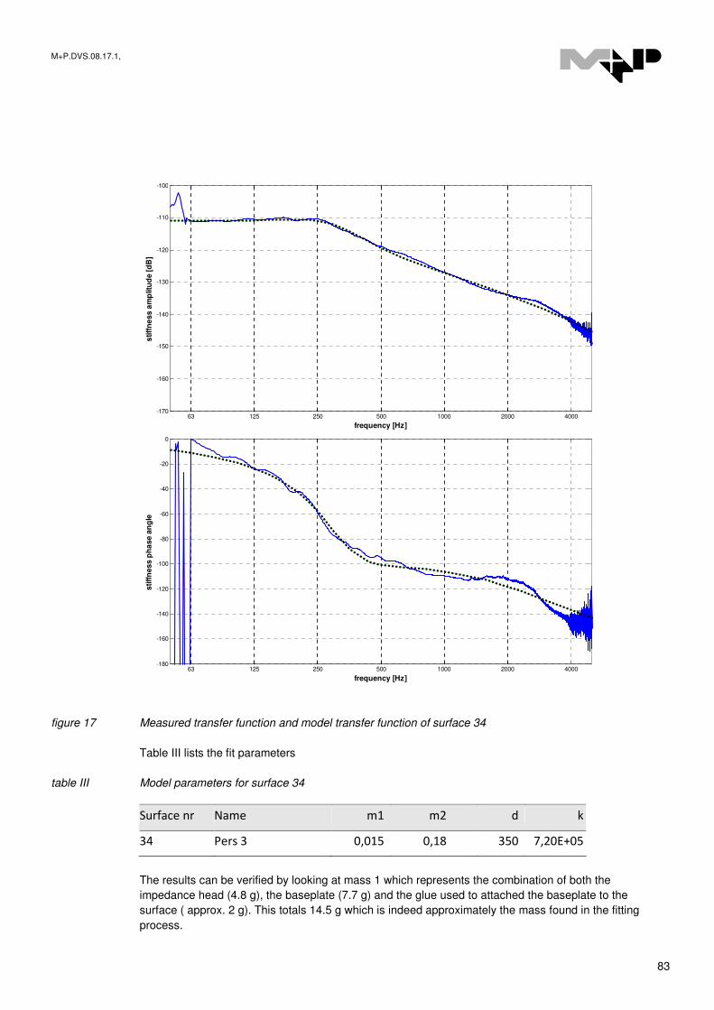
M+P.DVS.08.17.1,

83

63 125 250 500 1000 2000 4000-170

-160

-150

-140

-130

-120

-110

-100

frequency [Hz]

stiff

ne

ss a

mp

litu

de [

dB

]

63 125 250 500 1000 2000 4000-180

-160

-140

-120

-100

-80

-60

-40

-20

0

frequency [Hz]

sti

ffn

ess p

ha

se a

ng

le

figure 17 Measured transfer function and model transfer function of surface 34

Table III lists the fit parameters

table III Model parameters for surface 34

Surface nr Name m1 m2 d k

34 Pers 3 0,015 0,18 350 7,20E+05

The results can be verified by looking at mass 1 which represents the combination of both the

impedance head (4.8 g), the baseplate (7.7 g) and the glue used to attached the baseplate to the

surface ( approx. 2 g). This totals 14.5 g which is indeed approximately the mass found in the fitting

process.

M+P.DVS.08.17.1,

84

The model fitting procedure seems useful in further research into the dynamic characterization of

road surfaces. However, the fitting procedure is highly sensitive to errors and it should therefore be

automated. Additionally, more measurements at different spots on the surface should be performed

and averaged to obtain more accurate measuring results.

The impedance mass clearly influences the measurement results. This influence grows when the

mass of the impedance head and the characteristic mass of the surface are similar. Therefore, a

compensation technique should be applied [14]. This compensation is subject to current research.

M+P.DVS.08.17.1,

85

5 Skid resistance

5.1 Background

Skid resistance is an important safety consideration in the selection of road surfaces nowadays.

Skid resistance is highly related to tyre characteristics. However, road properties can also have a

significant effect. Skid resistance is generally associated with micro-texture of the road surface. On

wet surfaces, the effect of texture and other surface properties become increasingly important as

they facilitate the drainage of water. Wet skid resistance is hard to measure due to variable

conditions. Therefore, this study will only consider dry friction using a standard measuring method.


Skid resistance can be measured with the British pendulum test. The measurement setup is shown

in figure 18.

figure 18 British pendulum test setup

Under dry conditions the British pendulum test gives an indication of the friction coefficient of a road

surface which in turn gives an indication of micro texture. However, the values acquired by the

British pendulum have no absolute meaning and can only be used for relative comparison between

the road surfaces.


The averaged measurement results for surfaces 1 to 31 are shown in figure 19. The minimum and

maximum values of the skid resistance are indicated with the error bars.

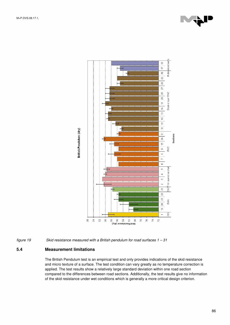
M+P.DVS.08.17.1,

86

figure 19 Skid resistance measured with a British pendulum for road surfaces 1 – 31

5.4 Measurement limitations

The British Pendulum test is an empirical test and only provides indications of the skid resistance

and micro texture of a surface. The test condition can vary greatly as no temperature correction is

applied. The test results show a relatively large standard deviation within one road section

compared to the differences between road sections. Additionally, the test results give no information

of the skid resistance under wet conditions which is generally a more critical design criterion.

M+P.DVS.08.17.1,

87

6 Tyre/road noise

6.1 Background

A number of road surface properties have been identified that influence tyre/road noise: road

texture, mechanical impedance and acoustic impedance. The acoustic impedance characterizes

the frequency dependent energy absorption of the road surface. This energy absorption is for

example influenced by the structure and the amount of voids in the road surface.

Tyre/road noise is an important factor in the selection of road surfaces nowadays. A number of

measuring methods are available to measure the noise exterior to the vehicle. In this study the

noise level is measured in close proximity of the tyre.


The tyre road noise is measured in close proximity (CPX) of the tyre with a structure containing 11 microphones (figure 20). This method is related to the Close Proximity (CPX) method, as described in ISO/CD 11819-2 [12]. For each microphone the A-weighted equivalent sound level LA,eq is measured (the overall level and the 1/3-octave bands between 50 and 5000 Hz) along with the vehicle speed.

figure 20 The close proximity measuring method to study tyre/road noise

A number of different tyres is used for the measurements and averaged for each road section.


It has been shown that there is a linear relation between velocity and tyre/road noise [13]. Therefore

a speed correction is applied prior to analysis. Figure 21 shows the sound levels of each section on

which a speed correction has been applied. The results clearly show the positive effect of the

flexible road surface on the tyre/road noise.

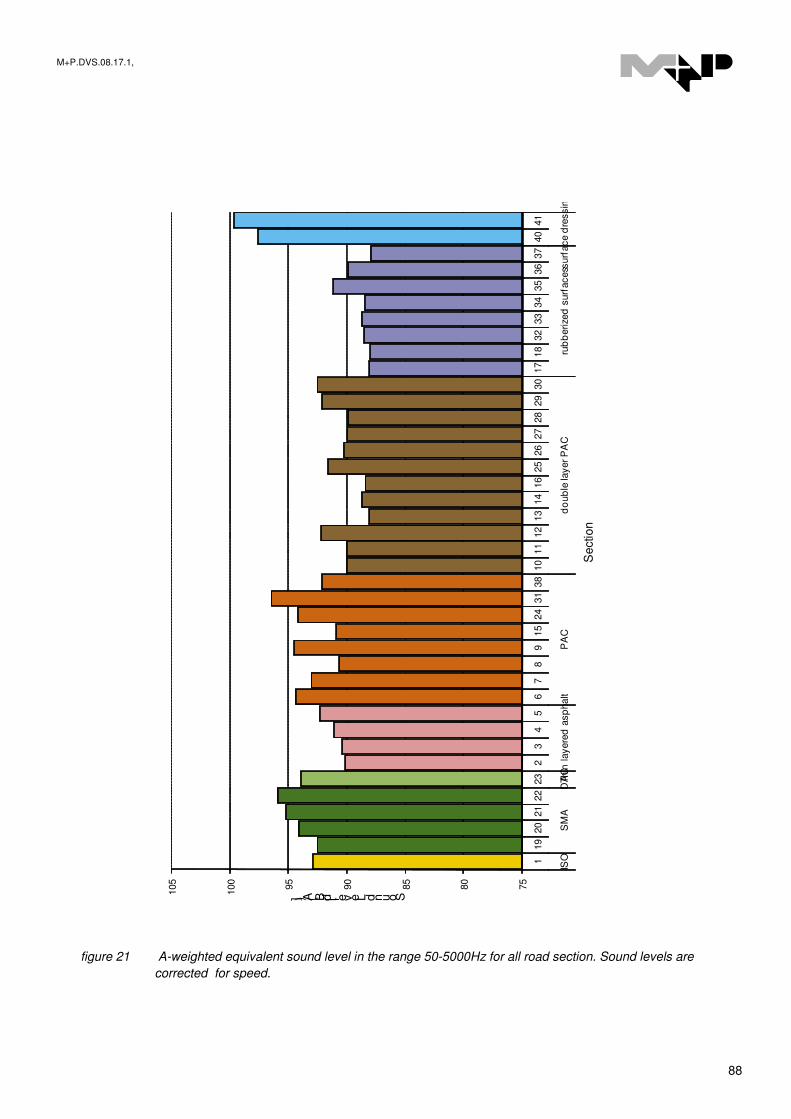
M+P.DVS.08.17.1,

88

75

80

85

90

95

100

105

119

20

21

22

23

23

45

67

89

15

24

31

38

10

11

12

13

14

16

25

26

27

28

29

30

17

18

32

33

34

35

36

37

40

41

ISO

SM

AD

AC

Thin

layere

d a

sp

halt

PA

Cd

oub

le la

yer P

AC

rub

berize

d s

urf

acess

urf

ace d

ressin

gs

Sound Level [dB(A)]

Se

ctio

n

figure 21 A-weighted equivalent sound level in the range 50-5000Hz for all road section. Sound levels are

corrected for speed.

M+P.DVS.08.17.1,

89

7 Regression analysis

The goal of this project is to find correlations between road surface properties and rolling

resistance. In Chapter 3, Chapter 4 and Chapter 5 a number of road surface properties is

described: road texture, mechanical impedance and skid resistance. This chapter studies empirical

relations between those properties and rolling resistance.

7.1 Influence of surface texture on rolling resistance

7.1.1 Texture amplitude characteristics

Figure 22 plots the root mean square (Rms) texture depth and the corresponding rolling resistance

coefficient for a Continental tyre on all surfaces. Each point represents a road surface and the

points are color coded according to the road category as shown in Appendix C. There appears to

be a clear correlation between rolling resistance and Rms texture depth. However, the rubberized

surfaces and the surface dressings do not correspond to this relation. Therefore, in subsequent

regression analysis these surfaces will be excluded.

Figure 22 also shows the linear regression trend line obtained by a least squares regression

procedure. The slope of the regression line is approximately 0.78 [1/mm] and the regression line

crosses the vertical axis at approximately 0.089. A correlation coefficient of R2=0.89 indicates a

rather good correlation between Rms texture depth and rolling resistance.

A t-test is applied to test whether the slope of the regression line differs significantly from zero (null-

hypothesis). Under the assumption of the null hypothesis the t-score is approximately 15.7 with 28

degrees of freedom. These values indicate that it is highly unlikely that there is in fact no

relationship between Rms texture depth and rolling resistance. Therefore, the null hypothesis has to

be rejected. Within a 95% confidence it can be stated that the slope of the regression line lies in the

interval [0.68;0.88].

It has to be noted that the correlation between Rms texture depth and rolling resistance does not

necessarily indicate a causal relationship between those two. However, it can be concluded that

selecting a conventional surface with 1 mm less Rms texture depth can give a reduction in rolling

resistance of approximately 7.5-10 % which results in a potential fuel reduction of approximately 1-

2%.

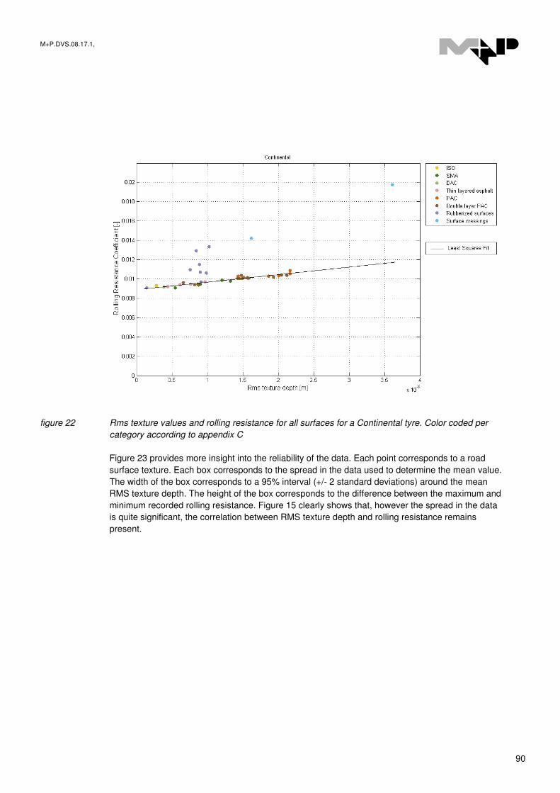
M+P.DVS.08.17.1,

90

figure 22 Rms texture values and rolling resistance for all surfaces for a Continental tyre. Color coded per

category according to appendix C

Figure 23 provides more insight into the reliability of the data. Each point corresponds to a road

surface texture. Each box corresponds to the spread in the data used to determine the mean value.

The width of the box corresponds to a 95% interval (+/- 2 standard deviations) around the mean

RMS texture depth. The height of the box corresponds to the difference between the maximum and

minimum recorded rolling resistance. Figure 15 clearly shows that, however the spread in the data

is quite significant, the correlation between RMS texture depth and rolling resistance remains

present.

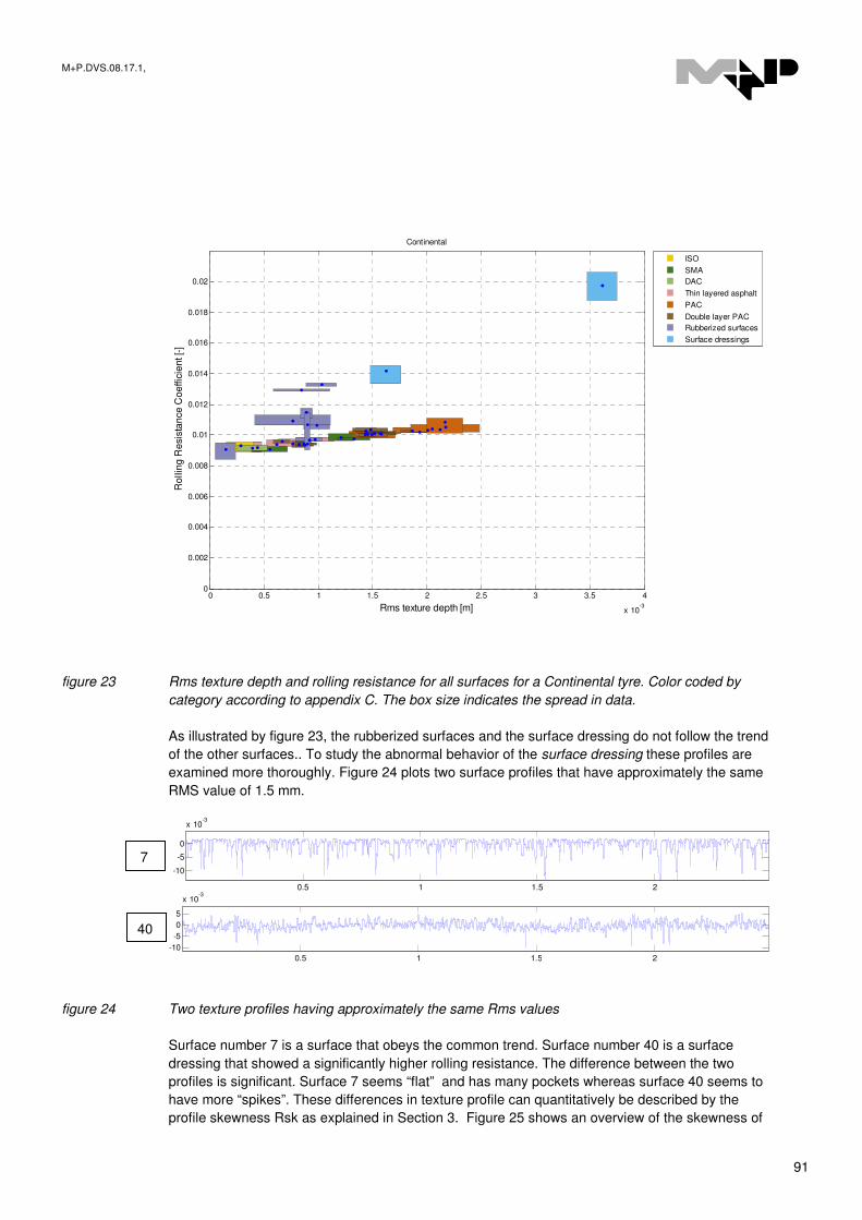
M+P.DVS.08.17.1,

91

0 0.5 1 1.5 2 2.5 3 3.5 4

x 10-3

0

0.002

0.004

0.006

0.008

0.01

0.012

0.014

0.016

0.018

0.02

Rms texture depth [m]

Ro

llin

g R

esis

tan

ce

Co

effic

ien

t [-

]

Continental

ISO

SMA

DAC

Thin layered asphalt

PAC

Double layer PAC

Rubberized surfaces

Surface dressings

figure 23 Rms texture depth and rolling resistance for all surfaces for a Continental tyre. Color coded by

category according to appendix C. The box size indicates the spread in data.

As illustrated by figure 23, the rubberized surfaces and the surface dressing do not follow the trend

of the other surfaces.. To study the abnormal behavior of the surface dressing these profiles are

examined more thoroughly. Figure 24 plots two surface profiles that have approximately the same

RMS value of 1.5 mm.

0.5 1 1.5 2

-10

-5

0

x 10-3

0.5 1 1.5 2

-10

-5

0

5

x 10-3

figure 24 Two texture profiles having approximately the same Rms values

Surface number 7 is a surface that obeys the common trend. Surface number 40 is a surface

dressing that showed a significantly higher rolling resistance. The difference between the two

profiles is significant. Surface 7 seems “flat” and has many pockets whereas surface 40 seems to

have more “spikes”. These differences in texture profile can quantitatively be described by the

profile skewness Rsk as explained in Section 3. Figure 25 shows an overview of the skewness of

7

40

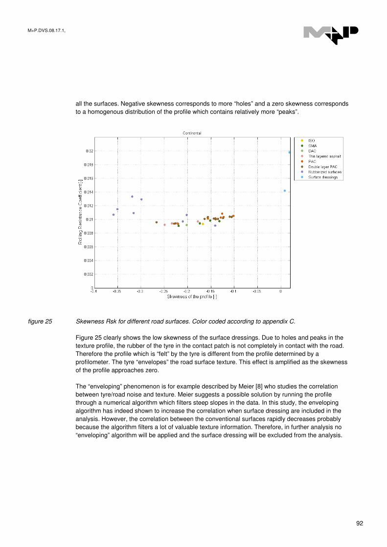
M+P.DVS.08.17.1,

92

all the surfaces. Negative skewness corresponds to more “holes” and a zero skewness corresponds

to a homogenous distribution of the profile which contains relatively more “peaks”.

figure 25 Skewness Rsk for different road surfaces. Color coded according to appendix C.

Figure 25 clearly shows the low skewness of the surface dressings. Due to holes and peaks in the

texture profile, the rubber of the tyre in the contact patch is not completely in contact with the road.

Therefore the profile which is “felt” by the tyre is different from the profile determined by a

profilometer. The tyre “envelopes” the road surface texture. This effect is amplified as the skewness

of the profile approaches zero.

The “enveloping” phenomenon is for example described by Meier [8] who studies the correlation

between tyre/road noise and texture. Meier suggests a possible solution by running the profile

through a numerical algorithm which filters steep slopes in the data. In this study, the enveloping

algorithm has indeed shown to increase the correlation when surface dressing are included in the

analysis. However, the correlation between the conventional surfaces rapidly decreases probably

because the algorithm filters a lot of valuable texture information. Therefore, in further analysis no

“enveloping” algorithm will be applied and the surface dressing will be excluded from the analysis.

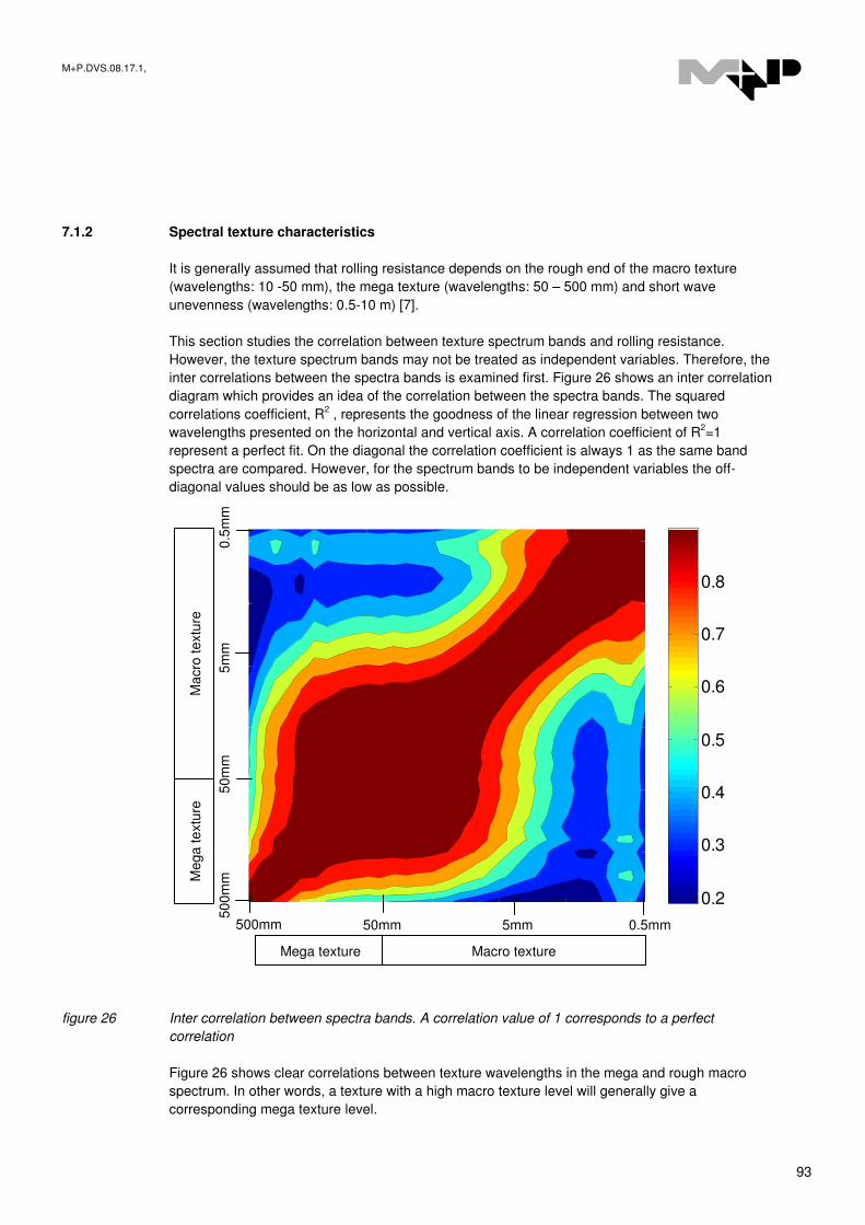
M+P.DVS.08.17.1,

93

7.1.2 Spectral texture characteristics

It is generally assumed that rolling resistance depends on the rough end of the macro texture

(wavelengths: 10 -50 mm), the mega texture (wavelengths: 50 – 500 mm) and short wave

unevenness (wavelengths: 0.5-10 m) [7].

This section studies the correlation between texture spectrum bands and rolling resistance.

However, the texture spectrum bands may not be treated as independent variables. Therefore, the

inter correlations between the spectra bands is examined first. Figure 26 shows an inter correlation

diagram which provides an idea of the correlation between the spectra bands. The squared

correlations coefficient, R2 , represents the goodness of the linear regression between two

wavelengths presented on the horizontal and vertical axis. A correlation coefficient of R2=1

represent a perfect fit. On the diagonal the correlation coefficient is always 1 as the same band

spectra are compared. However, for the spectrum bands to be independent variables the off-

diagonal values should be as low as possible.

5 10 15 20 25 30

5

10

15

20

25

30

0.2

0.3

0.4

0.5

0.6

0.7

0.8

figure 26 Inter correlation between spectra bands. A correlation value of 1 corresponds to a perfect

correlation

Figure 26 shows clear correlations between texture wavelengths in the mega and rough macro

spectrum. In other words, a texture with a high macro texture level will generally give a

corresponding mega texture level.

Mega texture Macro texture

Me

ga

te

xtu

re

Ma

cro

te

xtu

re

0.5

mm

5

0m

m

5m

m

50

0m

m

500mm 50mm 5mm 0.5mm

M+P.DVS.08.17.1,

94

Table IV indicates the correlations between the overall macro texture level Lma, mega texture level

Lme and the rolling resistance. Additionally the inter correlation between those two texture

parameter is presented.

table IV Correlation between macro texture, mega texture and rolling resistance

Linear regression Correlation coefficient R

Lma v.s. rolling resistance

0.91

Lme v.s. rolling resistance

0.90

Lma v.s. Lme 0.96

Table IV indeed shows that there is a strong correlation between both macro and mega texture and

rolling resistance. However, due to the strong inter correlation no conclusion can be drawn on the

relative influence of both texture regions.

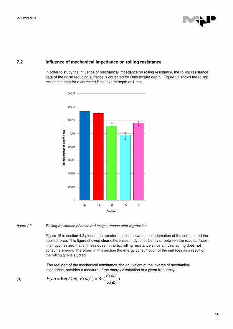
M+P.DVS.08.17.1,

95

7.2 Influence of mechanical impedance on rolling resistance

In order to study the influence of mechanical impedance on rolling resistance, the rolling resistance

data of the noise reducing surfaces is corrected for Rms texture depth. Figure 27 shows the rolling

resistance data for a corrected Rms texture depth of 1 mm.

0

0,002

0,004

0,006

0,008

0,01

0,012

0,014

0,016

32 33 34 35 36

Ro

llin

g r

esi

sta

nce

co

eff

icie

nt

[-]

Section

figure 27 Rolling resistance of noise reducing surfaces after regression

Figure 15 in section 4.3 plotted the transfer function between the indentation of the surface and the

applied force. This figure showed clear differences in dynamic behavior between the road surfaces.

It is hypothesized that stiffness does not affect rolling resistance since an ideal spring does not

consume energy. Therefore, in this section the energy consumption of the surfaces as a result of

the rolling tyre is studied.

The real part of the mechanical admittance, the equivalent of the inverse of mechanical

impedance, provides a measure of the energy dissipation at a given frequency:

(9) ))(

)(Re())()(Re()(

22

ω

ωωωω

Z

FFAP =⋅=

M+P.DVS.08.17.1,

96

Figure 28 plots the real part of the admittance as a function of the frequency. Given an input force

equal to 1 N the admittance gives a measure of the energy dissipation in Watts for given

frequencies.

63 125 250 500 1000 2000 4000-0.025

-0.02

-0.015

-0.01

-0.005

0

Frequency [Hz]

Re

al p

art

of

ad

mit

tan

ce

fo

r 1 N

in

pu

t [W

]

Surface 32

Surface 33

Surface 34

Surface 35

Surface 36

Porous Surface

figure 28 Power dissipation as a function of frequency for the six different surfaces.

Looking at figure 28 the question arises which frequency range affects the rolling resistance. The

tyre excites the surface in the contact patch. Figure 29 provides an indication of the surface

pressure profile within the contact patch.

figure 29 Pressure spectrum of a car tyre at the surface patch.

M+P.DVS.08.17.1,

97

The lowest frequency which could affect rolling resistance, fmin , is the frequency which corresponds

to the length of the contact patch lc at a given speed v

(10)

cl

vf =min

For a contact patch of 100 mm and a speed of 80 km/h this corresponds to a frequency of 222 Hz.

However, considering that the pressure only varies over a part of the contact patch lcp the maximum

frequency that could affect rolling resistance could be

(11)

cpl

vf =max

For lcp as one third of the contact patch (100 mm) and a speed of 80 km/h this corresponds to a

frequency of 666 Hz.

Combining figure 27, figure 28 and looking at the relevant frequency range there seems to be a

clear correlation between energy dissipation and rolling resistance. A higher energy dissipation in

the 250-400 Hz range appears to correspond to a higher rolling resistance. This result can

potentially be used in the design of new low rolling resistance, noise reducing and flexible road

surfaces.

It has to be noted that the relevant frequency range is highly dependent of the vehicle speed.

Therefore, it may be useful to measure the rolling resistance at varying speed to study this effect.

Additionally, the static stiffness of the road surface may cause a change in contact patch size and

may thereby shift the relevant frequency range. Further, decreasing the static stiffness potentially

lowers the resonant frequency which increases the energy dissipation at lower frequencies. These

topics should be further addressed in future research.

7.3 Correlation between skid resistance and rolling resistance.

Skid resistance is assumed to give an indication of the amount of micro texture on a surface. Figure

30 shows a scatter diagram of the skid resistance values obtained by a British Pendulum test and

the rolling resistance. From this figure it can be concluded that no clear correlation can be found

between skid resistance/micro texture and rolling resistance. Therefore, the requirements of

improving skid resistance and reducing rolling resistance do not conflict.

M+P.DVS.08.17.1,

98

figure 30 Skid resistance BPM values and rolling resistance..

Additional regression analysis with roughness on a wet road and vehicle deceleration has shown to

result in similar results. The absence of a significant relation can be related to the wavelength

dependency of both rolling resistance and grip. Grip is generally assumed to be affected by small

wavelengths, rolling resistance is generally affected by larger wavelengths (figure 8).

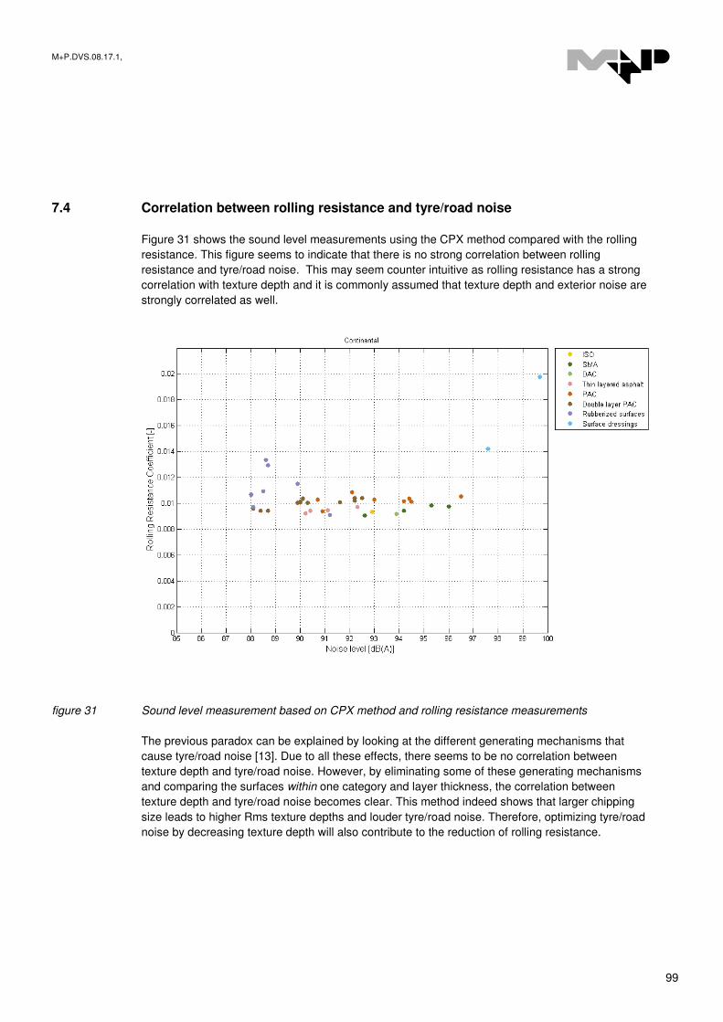
M+P.DVS.08.17.1,

99

7.4 Correlation between rolling resistance and tyre/road noise

Figure 31 shows the sound level measurements using the CPX method compared with the rolling

resistance. This figure seems to indicate that there is no strong correlation between rolling

resistance and tyre/road noise. This may seem counter intuitive as rolling resistance has a strong

correlation with texture depth and it is commonly assumed that texture depth and exterior noise are

strongly correlated as well.

figure 31 Sound level measurement based on CPX method and rolling resistance measurements

The previous paradox can be explained by looking at the different generating mechanisms that

cause tyre/road noise [13]. Due to all these effects, there seems to be no correlation between

texture depth and tyre/road noise. However, by eliminating some of these generating mechanisms

and comparing the surfaces within one category and layer thickness, the correlation between

texture depth and tyre/road noise becomes clear. This method indeed shows that larger chipping

size leads to higher Rms texture depths and louder tyre/road noise. Therefore, optimizing tyre/road

noise by decreasing texture depth will also contribute to the reduction of rolling resistance.

M+P.DVS.08.17.1,

100

8 Conclusion

This project focuses on the influence of road surface properties on rolling resistance. Additionally,

possible conflicting requirements concerning tyre/road noise and skid resistance are examined.

Measurements on rolling resistance, texture, mechanical impedance, skid resistance and tyre/road

noise are carried out on a test track with 41 different road surfaces in Kloosterzande. Amongst

those surfaces is a number of unconventional noise reducing surfaces. The rolling resistance

measurements are carried out with a specially designed trailer from the University of Gdansk

(Poland).

The observed rolling resistance coefficients are comparable to the ones found in literature. Outliers

come from rarely used and very rough surface dressings and unconventional flexible surfaces.

Some measurements appear to have a large spread which poses questions on the accuracy of the

results.

Strong correlations between texture spectra levels and rolling resistance are found in both macro

(wavelengths 0.5-50 mm) and mega (50 – 500 mm) texture regions. However, there appears to be

a strong inter-correlation between these texture regions and therefore the independent relative

influence remains unclear. Literature sources even suggest a stronger influence from shortwave

unevenness (wavelengths 0.5 – 5m) which is not observable with the current measurement setup.

Texture amplitude characteristics appear to have a good correlation with rolling resistance. Varying

Rms texture levels for conventional surfaces by 50% can have a reduction of the rolling resistance

of 7-10%. Outliers in this correlation are caused by rarely used surface dressings and flexible

rubber surfaces. The off-trend behavior of the surface dressing can probably be related to the non-

skew texture profiles.

For the flexible rubber surfaces the mechanical impedance is measured by excitation of the surface

using a shaker. A simple dynamic system is proposed to model the surface dynamics containing a

characteristic rubber mass. The acquired frequency response functions are reproducible and give

valuable information on the dynamic behavior of the surface. The real part of the admittance (the

inverse of the impedance) provides a measure of the frequency dependent energy dissipation. The

relevant frequency range is estimated to be 250-400 Hz. In this range, higher energy dissipation

corresponds with higher rolling resistance. Further research is required to determine the relevant

frequency range and to study the velocity dependency of the results. However, measuring

mechanical impedance seems to be a promising method for the analysis and optimization of flexible

road surfaces.

No conflicting requirements were found between skid resistance and rolling resistance. Skid

resistance is assumed to depend on micro texture levels (wavelengths <0.5mm). Rolling resistance

however depends on larger wavelengths. Further research is required to study the correlation

between wet skid resistance and rolling resistance.

No clear correlation can be found between rolling resistance and tyre/road noise. However,

amongst surfaces that share the same structure, a higher Rms texture depth will result in a higher

tyre/road noise level. Therefore, no conflicting requirements are found between lowering rolling

resistance and decreasing tyre/road noise.

M+P.DVS.08.17.1,

101

References

[1] Hans Bendtsen, European Commission, SILVIA PROJECT REPORT, Rolling Resistance, Fuel

Consumption and Emissions: A Literature Review, 2004.

[2] Ulf Sandberg, Road Macro- and Megatexture Influence on Fuel Consumption, Surface

Characteristics of Roadways: International Research and Technologies, ASTM STP 1031, W.E.

Meyer and J. Reichert, Eds., American Society for Testing and Materials, Philadelphia, 1990, pp.

460-479.

[3] Anita Ihs, Magnusson, Georg, 2000. The significance of various road surface properties for traffic

and surroundings. VTI notat, 71A – 2000. Swedish National Road and Transport Institute.

[4] Guy Descornet, Road Surface Influence on Tyre Rolling Resistance. Surface Characteristics of

Roadways: International Research and Technologies, ASTM STP 1031, W. E. Mayer and J.

Reichert, Eds., American Society for testing and Materials, Philadelphia, 1990, pp. 401-415

[5] P.D. Cenek, P.F. Shaw, Investigation of New Zealand Tyre/Road Interactions, Road Research

Bulletin,1990

[6] Ulf Sandberg, Jerzy A. Ejsmont, 2000, Noise emission, Friction and Rolling Resistance of car Tyres

– summary of an experimental study. Paper from NOISE-CON 2000, Newport Beach, California,

December 2000

[7] Ulf Sandberg, Jerzy A. Ejsmont, 2002, Tyre/Road reference book, Informex, SE-59040, Sweden

[8] A. von Meier, G.J. van Blokland, G. Descornet, The influence of texture and sound absorption on

the noise of porous road surfaces, 1992, Second International Symposium on Road surface

Characteristics

[9] ISO 8767. International Standard. Passenger car tyres – Methods of measuring rolling resistance.

Reference number ISO 8767:1992 (E)

[10] The Tyre, Rolling resistance and fuel savings, Societe de Technologie Michelin, Clermont-Ferrand,

2003

[11] ISO 13472. International Standard. Characterization of pavement texture by use of surface profiles.

Reference number: ISO 13473-1:1997(E)

[12] ISO 11819. International Standard. Method for measuring the influencceof road surfaces on traffic

noise – Part 2: “The close proximity method (CPX)”

[13] Acoustic Optimization Tool, M+P report DWW 06.04.08, November 2007

[14] O. Cakar, K.Y. Sanliturk, 2005, Elimination of transducer frequency response functions, Mechanical

Systems and Signal Precessing, Vol. 19, Issue 1, p.87-104

M+P.DVS.08.17.1,

102

APPENDIX A Road surfaces per category

M+P.DVS.08.17.1,

103

Section km Picture

Black/white squares are 1cm2

section 1

30 mm ISO-surface 12.855 – 12.935

section 2

25 mm Thin Layered

Asphalt 2/4

(12%)

12.935 – 13.016

section 3

25 mm Thin Layered

Asphalt 2/6

(8%)

13.016 – 13.096

section 4

25 mm Thin Layered

Asphalt 2/6

(12%)

13.096 – 13.177

section 5

25 mm Thin Layered

Asphalt 4/8

(12%)

13.177 – 13.257

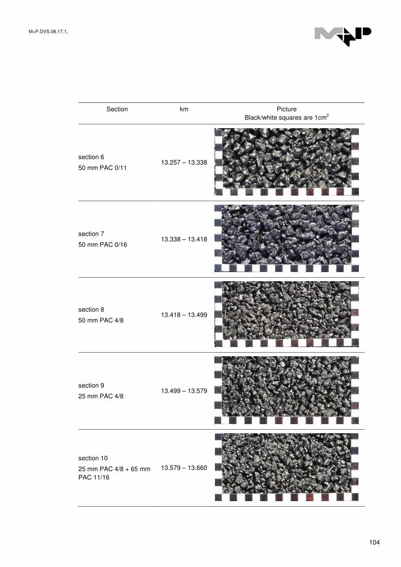
M+P.DVS.08.17.1,

104

Section km Picture


section 6

50 mm PAC 0/11 13.257 – 13.338

section 7

50 mm PAC 0/16

13.338 – 13.418

section 8

50 mm PAC 4/8 13.418 – 13.499

section 9

25 mm PAC 4/8 13.499 – 13.579

section 10

25 mm PAC 4/8 + 65 mm

PAC 11/16

13.579 – 13.660

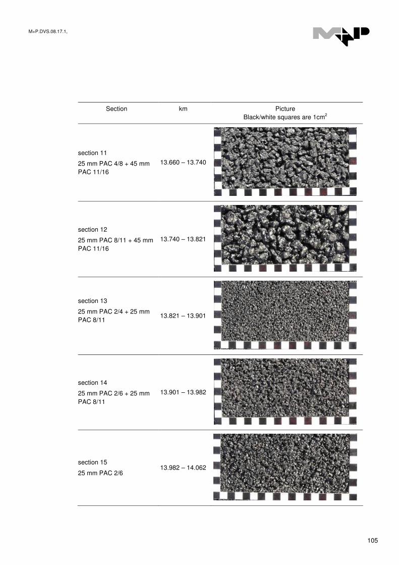
M+P.DVS.08.17.1,

105

Section km Picture


section 11

25 mm PAC 4/8 + 45 mm

PAC 11/16

13.660 – 13.740

section 12

25 mm PAC 8/11 + 45 mm

PAC 11/16

13.740 – 13.821

section 13

25 mm PAC 2/4 + 25 mm

PAC 8/11

13.821 – 13.901

section 14

25 mm PAC 2/6 + 25 mm

PAC 8/11

13.901 – 13.982

section 15

25 mm PAC 2/6 13.982 – 14.062

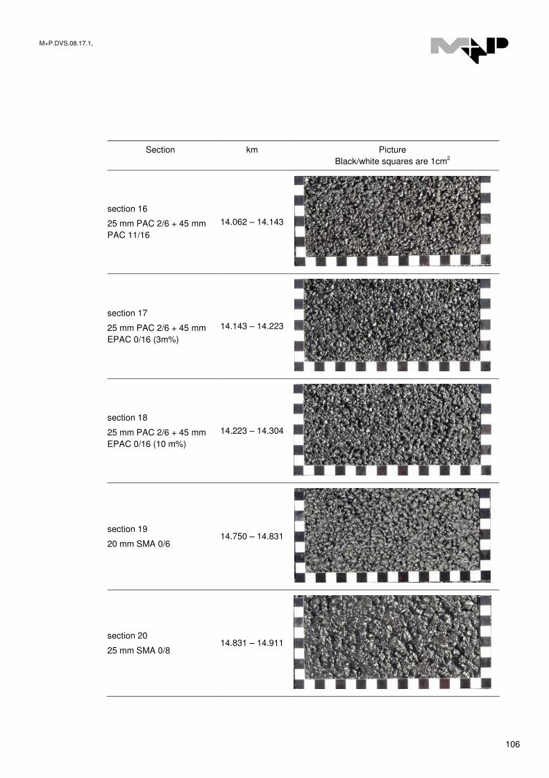
M+P.DVS.08.17.1,

106

Section km Picture


section 16

25 mm PAC 2/6 + 45 mm

PAC 11/16

14.062 – 14.143

section 17

25 mm PAC 2/6 + 45 mm

EPAC 0/16 (3m%)

14.143 – 14.223

section 18

25 mm PAC 2/6 + 45 mm

EPAC 0/16 (10 m%)

14.223 – 14.304

section 19

20 mm SMA 0/6 14.750 – 14.831

section 20

25 mm SMA 0/8 14.831 – 14.911

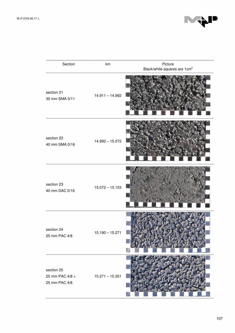
M+P.DVS.08.17.1,

107

Section km Picture


section 21

30 mm SMA 0/11 14.911 – 14.992

section 22

40 mm SMA 0/16 14.992 – 15.072

section 23

40 mm DAC 0/16 15.072 – 15.153

section 24

25 mm PAC 4/8 15.190 – 15.271

section 25

25 mm PAC 4/8 +

25 mm PAC 4/8

15.271 – 15.351

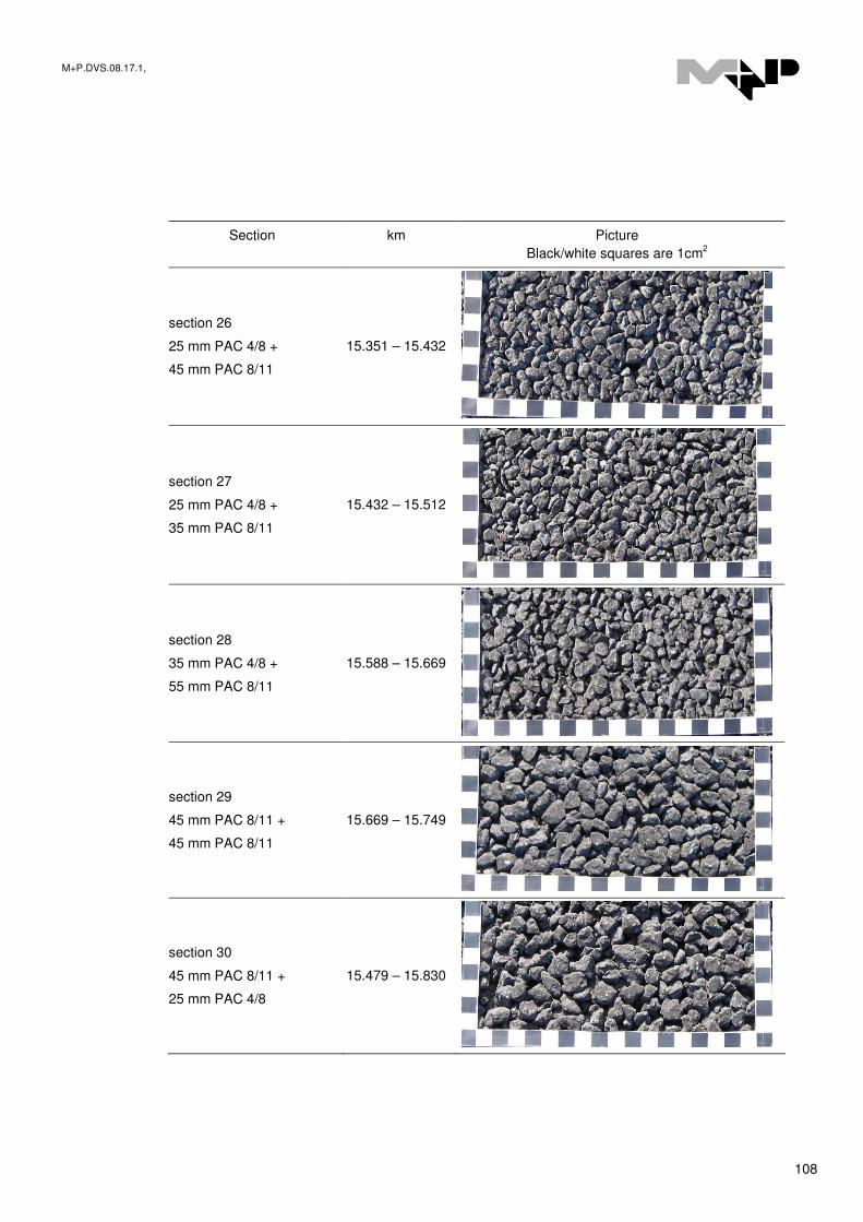
M+P.DVS.08.17.1,

108

Section km Picture


section 26

25 mm PAC 4/8 +

45 mm PAC 8/11

15.351 – 15.432

section 27

25 mm PAC 4/8 +

35 mm PAC 8/11

15.432 – 15.512

section 28

35 mm PAC 4/8 +

55 mm PAC 8/11

15.588 – 15.669

section 29

45 mm PAC 8/11 +

45 mm PAC 8/11

15.669 – 15.749

section 30

45 mm PAC 8/11 +

25 mm PAC 4/8

15.479 – 15.830

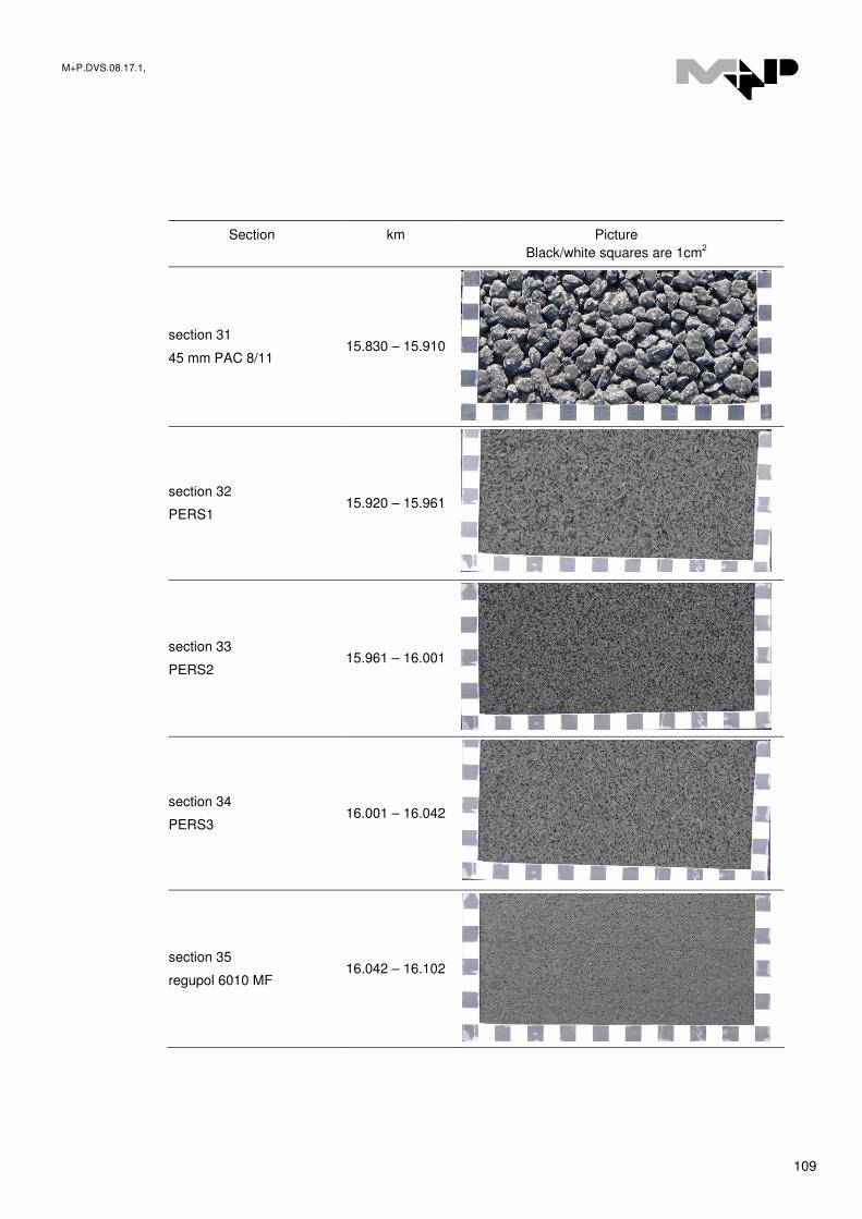
M+P.DVS.08.17.1,

109

Section km Picture


section 31

45 mm PAC 8/11 15.830 – 15.910

section 32

PERS1 15.920 – 15.961

section 33

PERS2 15.961 – 16.001

section 34

PERS3 16.001 – 16.042

section 35

regupol 6010 MF 16.042 – 16.102

M+P.DVS.08.17.1,

110

Section km Picture


section 36

regupol 6510 G 16.102 – 16.163

section 37

regupol 6510 G +

45 mm PAC 11/16

16.163 – 16.223

section 38

200 mm PAC 8/11 16.223 – 16.284

section 39

acoustic intermediate

section

16.284 – 16.314

section 40

5/8 surface dressing 16.314 – 16.375

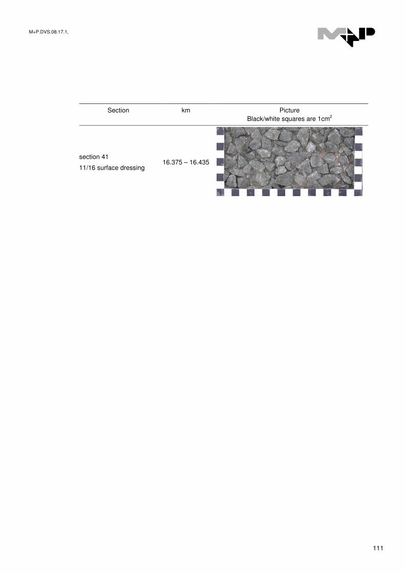
M+P.DVS.08.17.1,

111

Section km Picture


section 41

11/16 surface dressing 16.375 – 16.435

M+P.DVS.08.17.1,

112

APPENDIX A Rolling resistance measurements

M+P.DVS.08.17.1,

113

Surface 1

Surface 2

Surface 3

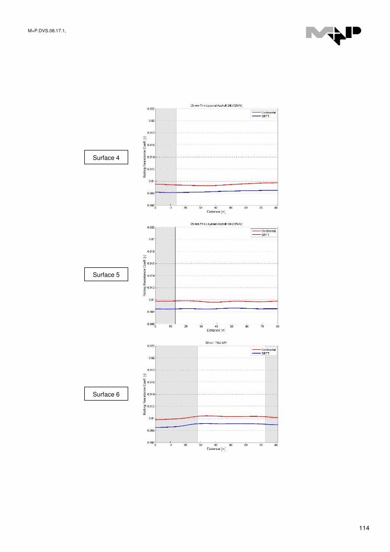
M+P.DVS.08.17.1,

114

Surface 4

Surface 5

Surface 6

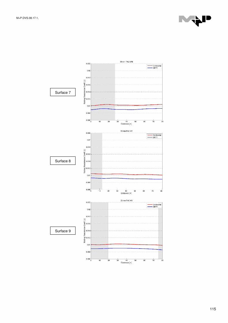
M+P.DVS.08.17.1,

115

Surface 7

Surface 8

Surface 9

M+P.DVS.08.17.1,

116

Surface 10

Surface 11

Surface 12

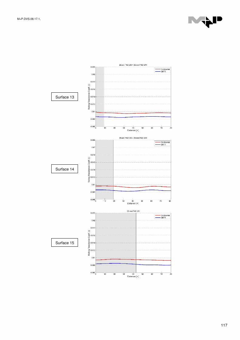
M+P.DVS.08.17.1,

117

Surface 13

Surface 14

Surface 15

M+P.DVS.08.17.1,

118

Surface 16

Surface 17

Surface 18

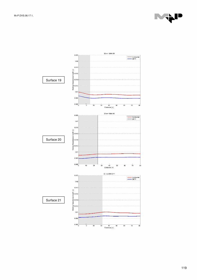
M+P.DVS.08.17.1,

119

Surface 19

Surface 20

Surface 21

M+P.DVS.08.17.1,

120

Surface 22

Surface 23

Surface 24

M+P.DVS.08.17.1,

121

Surface 25

Surface 26

Surface 27

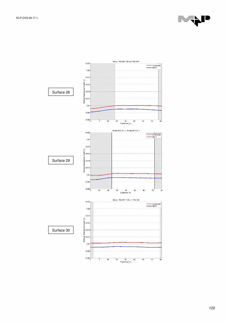
M+P.DVS.08.17.1,

122

Surface 28

Surface 29

Surface 30

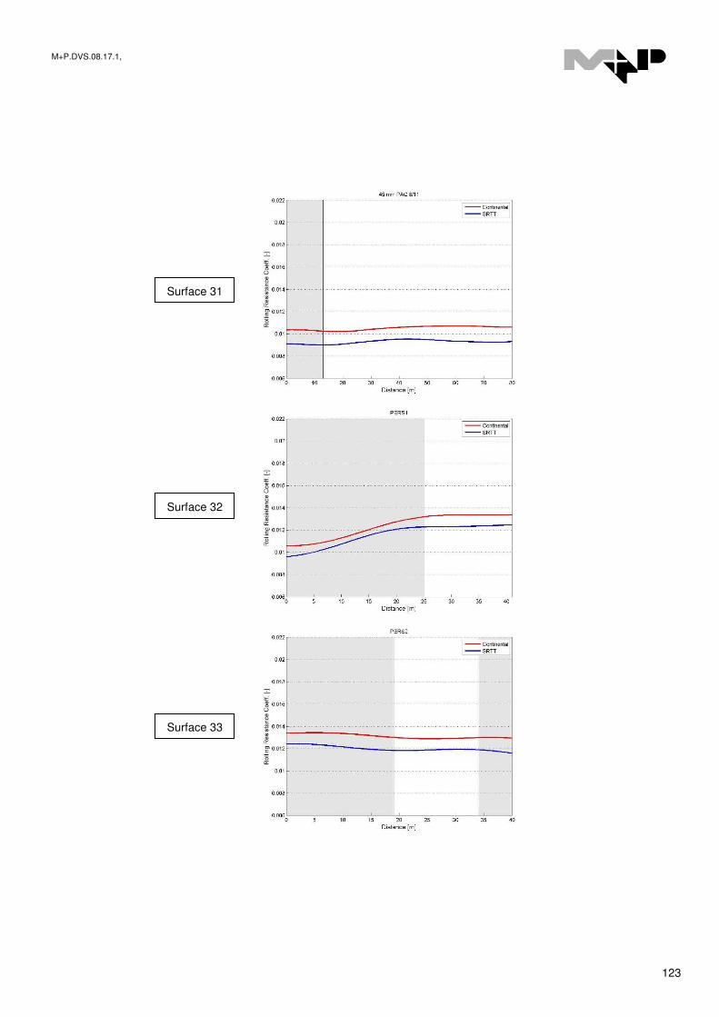
M+P.DVS.08.17.1,

123

Surface 31

Surface 32

Surface 33

M+P.DVS.08.17.1,

124

Surface 34

Surface 35

Surface 36

M+P.DVS.08.17.1,

125

Surface 37

Surface 38

Surface 40

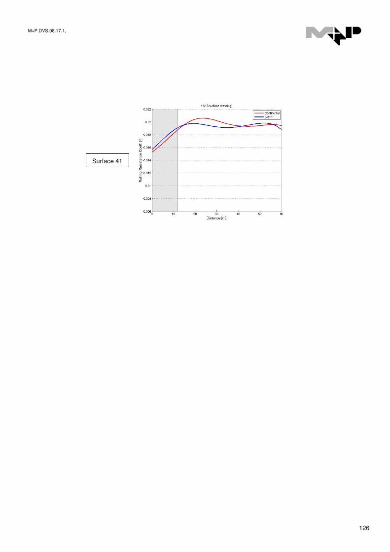
M+P.DVS.08.17.1,

126

Surface 41

M+P.DVS.08.17.1,

127

APPENDIX B Road surfaces per category

M+P.DVS.08.17.1,

128

ISO 1 ISO-10844

19 20 mm SMA 0/6

20 25 mm SMA 0/8

21 30 mm SMA 0/11

22 40 mm SMA 0/16

DAC 23 40 mm DAC 0/16

2 thin porous layer 2/4, 12%




6 50 mm PAC 0/11

7 50 mm PAC 0/16

8 50 mm PAC 4/8

9 25 mm PAC 4/8

15 25 mm PAC 2/6

24 25 mm PAC 4/8

31 45 mm PAC 8/11

38 200mm PAC 8/11

10 25 mm PAC 4/8 - 65 mm PAC 11/16

11 25 mm PAC 4/8 - 45 mm PAC 11/16

12 25 mm PAC 8/11 - 45 mm PAC 11/16

13 25 mm PAC 2/4 - 25 mm PAC 8/11

14 25 mm PAC 2/6 - 25 mm PAC 8/11

16 25 mm PAC 2/6 - 45 mm PAC 11/16

25 25 mm PAC 4/8 + 25 mm PAC 4/8

26 25 mm PAC 4/8 + 45 mm PAC 8/11

27 25 mm PAC 4/8 + 35 mm PAC 8/11

28 35 mm PAC 4/8 + 55 mm PAC 8/11

29 45 mm PAC 8/11 + 45 mm PAC 8/11

30 45 mm PAC 8/11 + 25 mm PAC 4/8

17 25 mm PAC 2/6 - 45 mm EPAC 0/16 (3m%)

18 25 mm PAC 2/6 - 45 mm EPAC 0/16 (10m%)

32 PERS1

33 PERS2

34 PERS3

35 15 mm Regupol 6010 MF

36 15 mm Regupol 6510 G

37 15 mm Regupol 6510 G + 55 mm PAC 11/16

40 5/8 surface dressing

41 11/16 surface dressing

SMA

Thin layered asphalt

PAC

double layer PAC

rubberized surfaces

surface dressings

prediction of road texture inﬂuence on rolling resistance · chapter2 literaturereview rolling...

Documents