1

Prediction of Pile Set-Up for

Ohio Soils

Lutful I. Khan Ph.D., P.E. Kirk Decapite

Prepared for the

Ohio Department of Transportation Office of Research and Development

State Job Number 134415

February 2011

Prepared in cooperation with the Ohio Department of Transportation and the U.S. Department Transportation, Federal Highway Administration.

2

1. Report No.

FHWA/OH-2011/3 2. Government Accession No. 3. Recipient's Catalog No.

4. Title and subtitle

Predicitin of Pile Set-up for Ohio Soils

5. Report Date

February 2011

6. Performing Organization Code

7. Author(s)

Lutful Khan, PhD, PE Kirk Decapite

8. Performing Organization Report No.

10. Work Unit No. (TRAIS) 9. Performing Organization Name and Address

Cleveland State University Civil & Environmental Engineering Cleveland, OH 44115

11. Contract or Grant No.

134415

13. Type of Report and Period Covered 12. Sponsoring Agency Name and Address

Ohio Department of Transportation 1980 West Broad Street Columbus, Ohio 43223 14. Sponsoring Agency Code

15. Supplementary Notes

16. Abstract

ODOT typically uses small diameter driven pipe piles for bridge foundations. When a pile is driven into the subsurface, it disturbs and displaces the soil. As the soil surrounding the pile recovers from the installation disturbance, a time dependant increase in pile capacity often occurs due to pile set-up. A significant increase in pile capacity could occur due to the set-up phenomenon. For optimization of the pile foundations, it is desirable to incorporate set-up in the design phase or predict the strength gain resulting from set-up so that piles could be installed at a lower End of Initial Driving (EOID) capacity. In order to address the set-up phenomena in Ohio geology, a research was conducted by compiling pile driving data in Ohio soils obtained from ODOT and GRL, an engineering company dedicated to dynamic pile load testing, located in Cleveland, Ohio. The set-up data of twenty three piles was compiled along with time, pile length, pile diameter. The liquid limit, plastic limit, average clay and silt content, average SPT value were compiled along the pile length. In 91 % cases of the driven piles, some degree of set-up was observed. Correlations among several soil parameters and pile capacities were explored. An equation was proposed between the final and initial load capacities of the piles as a function of time and shown to be in good agreement with the strength gains of driven pipe piles in Ohio soils.

17. Key Words

Pile set-up in Ohio Soils, Pile set-up, Set-up equation, relaxation, implementation.

18. Distribution Statement No restrictions. This document is available to the public through the National Technical Information Service, Springfield, Virginia 22161

19. Security Classif. (of this report)

Unclassified

20. Security Classif. (of this page)

Unclassified 21. No. of Pages : 34

22. Price

Form DOT F 1700.7 (8-72) Reproduction of completed pages authorized

3

Prediction of Pile Set-Up for Ohio Soils

Lutful I. Khan Ph.D., P.E. Associate Professor

Civil & Environmental Engineering Department Cleveland State University

Cleveland, Ohio 44115 Email: l.khan@csuohio.edu

Tel: 216-687-2231

Kirk Decapite Graduate Assistant

Civil & Environmental Engineering Department Cleveland State University

Cleveland, Ohio 44149

February 2011

Prepared in cooperation with the Ohio Department of Transportation and the U.S. Department Transportation, Federal Highway Administration.

The contents of this report reflect the views of the authors who are responsible for the facts and the accuracy of the data presented herein. The contents do not necessarily reflect the official views or policies of the Ohio Department of Transportation or the Federal Highway Administration. This report does not constitute a standard, specification or regulation.

4

Table of Contents Introduction ..................................................................................................................................... 5

Objectives of the Study ................................................................................................................... 6

Importance of Pile Set-up ................................................................................................................ 6

Literature Review ............................................................................................................................ 6

The Set-up Phenomenon................................................................................................................ 13

Pile Set-up Equations ................................................................................................................ 13

Analysis of Set-up Behavior ........................................................................................................... 15

Soil Characteristics .................................................................................................................... 15

EOID and Restrike Capacities..................................................................................................... 17

Set-up evaluation criteria .......................................................................................................... 19

Effect of length .......................................................................................................................... 20

Effect of clay and silt content .................................................................................................... 22

Effect of Standard Penetration Test (SPT) value ....................................................................... 24

Effect of Restrike Time on Set-up rate ...................................................................................... 25

Predicting Pile Set-up .................................................................................................................... 27

Implementation ............................................................................................................................. 28

Pile Design ................................................................................................................................. 30

Site Characterization ..................................................................................................................... 31

Conclusions .................................................................................................................................... 31

Acknowledgements ....................................................................................................................... 32

REFERENCES .................................................................................................................................. 32

5

Introduction

ODOT typically uses small diameter steel driven pipe piles for bridge

foundations. When a pile is driven into the subsurface, it disturbs and displaces the soil.

As the soil surrounding the pile recovers from the installation disturbance, a time

dependant increase in pile capacity often occurs. This phenomenon is referred to as “set-

up” or “pile freeze”. A significant increase in pile capacity could occur due to the set-up

phenomenon. For optimization of the pile foundations, it is desirable to incorporate set-up

in the design phase or predict the strength gain resulting from set-up so that piles could be

installed at a lower End of Initial Driving (EOID) capacity.

Different mechanisms have been proposed to explain set-up phenomenon in sand,

clay and mixed soils. However, set-up cannot be predicted based on the knowledge of the

engineering properties of soil. In engineering practice, set-up is incorporated in the design

phase during static analysis. The uncertainty remains whether set-up will occur at the site.

Because of many uncertainties associated with pile foundation analysis and design, full-

scale pile load tests are often carried out at the field. During the construction phase, set-

up could be calculated using empirical equations used in conjunction with dynamic test

methods. Dynamic test methods involve measurements of force and velocity near the pile

head taken during initial driving and subsequently during restrike. These measurements

can be used to estimate pile capacity among other attributes like performance of the pile

driving system, pile installation stresses and pile integrity. Soil set-up can be determined

by comparing restrike capacity with the EOID capacity obtained from dynamic testing.

Once set-up has been characterized, it could be applied to optimize the piles.

Although reported to be common, set-up does not occur in all soil strata. In some

soils, though rarely, a reverse phenomenon called “relaxation” may occur where the pile

looses capacity with time. It is therefore important to understand the set-up in the context

of local geology to take advantage of it.

6

Pile set-up mechanism is not fully understood. It is frequently observed in Ohio

soils at the ODOT construction sites. In order to address the set-up phenomena in Ohio

geology, a research was conducted by compiling pile driving data from ODOT and GRL,

an engineering company dedicated to dynamic pile load testing, located in Cleveland,

Ohio.

Objectives of the Study

Set-up is frequently observed in driven piles constructed in Ohio. The central

objective of the proposed research was to evaluate this phenomenon specific to the

region. Data from pile installations and subsequent load tests were collected and

compiled. Set-up in those sites was identified and attempt was made to characterize the

set-up phenomena in terms of known parameters. Alternatively, if it was determined that

no significant change in strength occurred following pile installation in a particular strata,

the objective was to provide all documentation to identify that condition during the

design phase.

Importance of Pile Set-up

Principal factors such as soil type, pile material and its installation method affect

soil/pile set-up. If the increment of pile capacity with time is taken into consideration,

benefits such as smaller pile section (diameter), shorter pile length, and lower capacity of

driving equipment will be required. Subsequently, shorter piling duration will lead to

overall cost reduction of piling work. All these reductions will considerably lower

overall cost of an ODOT project that involves pile driving.

Literature Review

The history of pile set-up dates back to about hundred years. Several literatures related to

pile set-up were identified and reviewed. The following section provides a summary of the

papers.

“Measured Pile Setup During Load Testing and Production Piling: I-15

Corridor Reconstruction Project in Salt Lake City, Utah.” [1]

Testing was performed on piles along the I-15 Corridor in Salt Lake City,

Utah. They noted that set-up in clays was attributed to remolding of the clays

during pile driving and subsequent reconsolidation. A dynamic test was

performed to determine long term pile capacity. Pile set-up had occurred

regardless of the subsurface conditions. A more rapid strength gain was

observed in soils with inter-bedded granular strata.

“Dynamic Pile Response Using Two Pile-Driving Techniques.” [2]

7

This paper discussed a method of driving piles by dropping the hammer inside

of the pile. Thus the pile was pulled into the ground instead of being pushed.

This was proven to be a more efficient method of pile installation.

“A Study of the Setup Behavior of Drilled Shafts.” [3]

A study was conducted on drilled shafts to characterize their set-up. The

drilled shafts were constructed of reinforced concrete with 5 to 9 ft. in

diameter. The shafts were driven to a depth of 50 ft. The authors concluded

that there was no correlation between pile length and set-up. The drilled shafts

showed set-up but little. The “A” values ranged from 0.38 to 0.1. The data

was compared with driven precast piles. The precast piles showed more set-up

with an “A” factor of 0.58.

“Side Shear Setup I: Test Piles Driven in Florida.” [4]

This study was conducted by the University of Florida. The purpose was to

determine the set-up on the side of the pile shaft known as “side shear setup”

(SSS). The piles were 18 in square, prestressed concrete. The Skov & Denver

(1988) equation was used to evaluate SSS. This paper believed that the cause

of setup was horizontal effective stresses or consolidation which increased

pile-soil adhesion. CAPWAP was used to determine side shear side-up and the

O-cell measure the pore water pressure. Using SSS they determined a value

for “A” with a range of 0.12 to 0.32. They have also reported that static and

dynamic tests showed similar results.

“Side Shear Setup II: Test Piles Driven in Florida.” [5]

This paper reviewed details of the University of Florida‟s pile testing and

determined a side shear setup test (SSS). This paper then proposed a

procedure to incorporate SSS. It was noted that cohesive soils continued to

increase in strength after the pore water pressure dissipated. Using standard

penetration test (SPT) with a torque measurement they determined this test to

be accurate and practical for determining pile set-up. This test was then

verified by determining the “A” value from the Skov and Denver (1988)

equation with to equal to one day. “A” was determined to be in the range of

0.2 to 0.8. If a predictor test is not performed “A” should default to 0.1.

“Time-related Increase in Shaft Capacities of Driven Piles in Sand.” [6]

This paper discussed pile set-up that occurred at Dunkirk in Northern France.

The piles were steel open-ended piles being driven into sand. The rise in

capacity was measured at 70% within 20 days after installation. After twenty

8

days the pile didn‟t experience additional set-up. The authors concluded that a

pause of at least 20 days is recommended to allow the pile to set-up. Thus

capacities determined at installation will not be the same for long term

capacity. The author believes changes in the stress regime caused by pile

installation caused set-up.

“Numerical Simulation of Pile Installation and Set-up.” [7]

This research investigated pile set-up which included a brief history and

typical methods. It was noted that the Wisconsin DOT has incorporated set-up

into bridge design with the use of preconstruction pile load tests. This paper

looked more at the stresses in the soil using a finite element analysis. The

belief was the stress was caused by pore pressure and earth pressure/stresses.

“Dynamic and Static Testing in Soil Exhibiting Set-Up.” [8]

This paper looked at four different steel piles driven into a group. The piles

were driven to a depth of 150 ft. The soil profile was;

1) Miscellaneous earth fills

2) Soft to medium stiff compressible silty clay

3) Glacial soil deposits

4) Dolomite bedrock

The test methods used to evaluate the piles were CAPWAP and static load

tests. This paper concluded that all piles showed set-up. With the use of

CAPWAP, set-up was determined.

“Static Loading Test on a 45 m Long Pipe Pile in Sandpoint, Idaho.” [9]

This paper focused on piles driven into soft compressible clay. The depth of

piles is between 80m to 200m. A test pile was driven a depth of 45m and

tested. The test pile showed that setup occurs rapidly fast in the soft clay. A

similar result was determined in “Measured Time Effects for Axial Capacity

of Driven Piling” where greater set-up was noticed in soft clay. The down side

to soft clay was it showed little pile capacity. With this test data they were

able to apply it to piles with longer lengths and larger diameters.

“Bridge Piles: More Capacity over Time?” [11]

This study discussed the basics of pile set-up. The paper believed pile set-up

was related to pore water pressure. Directly testing piles could be costly but

using subsurface information would help determine pile set-up. They

determined that the Test-Torque-Test was a measure of set-up between

sampler and soil. This was measured using a standard split barrel driven into

the soil.

9

“Dynamic Testing of Pile Foundations During Construction.” [13]

This paper discussed testing of piles and how static load test was a time

consuming expensive method of testing. Dynamic testing could provide

accurate values for pile capacity. The dynamic test was evaluated using Pile

Driving Analyzer (PDA) and Case Pile Wave Analysis Program (CAPWAP).

This paper concluded that dynamic testing was a more efficient method of

testing piles.

“Simulated Pile Load-Movement Incorporation Anticipated Soil Set-up.” [14]

This paper discussed the different methods of testing pile capacity in the field.

The two methods used were Pile Driving Analyzer (PDA) and CAPWAP.

These results were then verified through static load tests. The piles tested were

closed end typically used for a bridge. The soil conditions were sand and clay

mix. The authors concluded that dynamic testing was an accurate method of

testing piles when compared to static load test. CAPWAP was utilized to

determine set-up.

”Incorporation Set-up and Support Cost Distributions into Driven Pile

Design.” [15]

This paper discussed pile set-up basics related to the depth of the pile. Similar

to Florida DOT, Van E. Komurka (WisDOT consultant) believes set-up

occurred along the shaft of the pile. Thus the longer the pile the more set-up

will be experienced.

“Incorporating Set-up into Driven Pile Design and Installation.” [16]

This paper investigated set-up as a function of depth. It concluded that up to

50% of long-term capacity could be attributed to set-up. The use of dynamic

monitoring with set-up data could be used to predict pile capacity as a

function of depth.

“Value of Methods for Predicting Axial Pile Capacity.” [17]

This paper used a variety of dynamic formulas to predict pile capacity. The

main formulas were ME, PDA, WEAP, and CAPWAP. CAPWAP was

ultimately the combination of WEAP and PDA testing. This paper concluded

that the ME method was the most precise measurement when only EOD data

was used. When CAPWAP was used in combination with BOR test it had the

greatest precision.

“Measured Time Effects for Axial Capacity of Driven Piling.” [18]

The purpose of this paper was to determine causes of set-up based on pile

testing data. The soils were sand, primarily clay, and mixed soil. An important

observation made is that strength gain continued after pore water pressure had

10

dissipated. They termed this “aging”. Piles driven into soft clay tend to

experience greater set-up than piles driven into stiff clay. Piles driven into

saturated, dense sand and silts or into shale may experience relaxation. This

paper concluded that setup in clay experienced strength gain from 1-6 times

after driving. Only a few cases of relaxation were found and were determined

to be a rare occurrence.

“Driven Piles in Clay – the Effects of Installation and Subsequent

Consolidation.” [19]

This paper used numerical analysis to predict pile capacity. By modeling a

pile, they were able to determine the stress on a pile, including stress changes.

The changes in stress were attributed to consolidation of the soil around the

pile and expansion of the cavity. This paper concluded that shaft capacity was

not affected by over consolidation ratio of the soil. Further research was

suggested to determine that fact.

“Dynamic Determination of Pile Capacity.” [20]

This paper was conducted with the help of the Michigan Highway

Department. The purpose was to determine whether dynamic testing was an

accurate test method for determining pile capacity. This paper concluded that

CAPWAP was an accurate method of determining the static capacity of a pile.

“On the Prediction of Long Term Pile Capacity from End-of-Driving

Information,” [21]

The focus was to determine an accurate method of testing and predicting pile

capacity from end-of-drive data. This capacity could then be used to

determine pile set-up, or “long term capacity”. By determining accurate pile

set-up, the design of piles would be less conservative and more economical. A

less conservative pile would result in shorter piles with smaller diameters.

According to the authors, the possible reasons for set-up included,

Change in pore water pressure caused by pile installation.

Liquefaction in loose granular soils due to the dynamic pile

motions and thus a greatly reduced effective stress.

Soil remolding as is frequently found in clays or thixotropic

materials.

Soil fatigue.

Loss of cement structure in calcareous soils.

Gradual cracking of rock underneath the pile toe due to very high

11

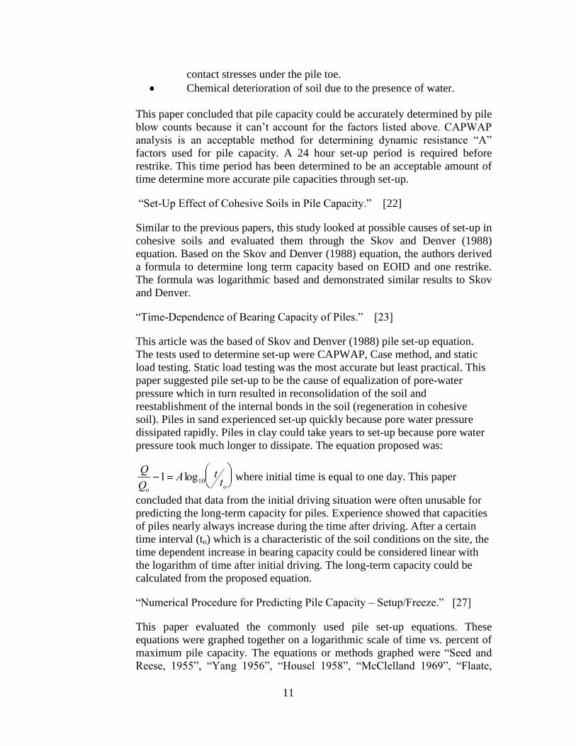
contact stresses under the pile toe.

Chemical deterioration of soil due to the presence of water.

This paper concluded that pile capacity could be accurately determined by pile

blow counts because it can‟t account for the factors listed above. CAPWAP

analysis is an acceptable method for determining dynamic resistance “A”

factors used for pile capacity. A 24 hour set-up period is required before

restrike. This time period has been determined to be an acceptable amount of

time determine more accurate pile capacities through set-up.

“Set-Up Effect of Cohesive Soils in Pile Capacity.” [22]

Similar to the previous papers, this study looked at possible causes of set-up in

cohesive soils and evaluated them through the Skov and Denver (1988)

equation. Based on the Skov and Denver (1988) equation, the authors derived

a formula to determine long term capacity based on EOID and one restrike.

The formula was logarithmic based and demonstrated similar results to Skov

and Denver.

“Time-Dependence of Bearing Capacity of Piles.” [23]

This article was the based of Skov and Denver (1988) pile set-up equation.

The tests used to determine set-up were CAPWAP, Case method, and static

load testing. Static load testing was the most accurate but least practical. This

paper suggested pile set-up to be the cause of equalization of pore-water

pressure which in turn resulted in reconsolidation of the soil and

reestablishment of the internal bonds in the soil (regeneration in cohesive

soil). Piles in sand experienced set-up quickly because pore water pressure

dissipated rapidly. Piles in clay could take years to set-up because pore water

pressure took much longer to dissipate. The equation proposed was:

Q

Qo1 Alog10

tto

where initial time is equal to one day. This paper

concluded that data from the initial driving situation were often unusable for

predicting the long-term capacity for piles. Experience showed that capacities

of piles nearly always increase during the time after driving. After a certain

time interval (to) which is a characteristic of the soil conditions on the site, the

time dependent increase in bearing capacity could be considered linear with

the logarithm of time after initial driving. The long-term capacity could be

calculated from the proposed equation.

“Numerical Procedure for Predicting Pile Capacity – Setup/Freeze.” [27]

This paper evaluated the commonly used pile set-up equations. These

equations were graphed together on a logarithmic scale of time vs. percent of

maximum pile capacity. The equations or methods graphed were “Seed and

Reese, 1955”, “Yang 1956”, “Housel 1958”, “McClelland 1969”, “Flaate,

12

1972”, “Thorburn and Ridgen 1980”, “Konrad and Roy 1987”, “McManis

1988”, “Skov and Denver 1988”, and “Fellenius et al 1989”. This paper

attempted to develop a general numerical procedure to determine pile-set.

When applied to full scale piles, the procedure could be used to develop a

graph for the area of piles dependant on pile type, size, and soil

characteristics.

“Increase in Shaft Capacity with Time for Friction Piles Driven Into Saturated

Clay.” [28]

Side friction of open and closed-end piles were evaluated. Full scale tests

were conducted on the piles with focus on the stress on the side or skin

friction. Numerical equations were applied to determine pile capacity and then

tested in the field.

“Prediction of Pile Setup in Clay” [29]

This paper explored creation of realistic models of piles in soil in order to

make accurate predictions of pile performance. This model would be related

to the behavior of the soil density. A Piezo model was used to determine

stresses, pore pressure, average skin friction, consolidation, and axial loading.

This model determined that set-up occurring in soft clays could be related to

the changes in radial effective stress that occur during installation and

subsequent radial dissipation of excess pore pressures. Radial stress was

believed to be dependent on pile geometry (open or closed end), OCR, and

strength properties at large shear strains.

“Incorporating Set-Up into Load and Resistance Factor Design of Driven Piles

in Sand.” [30]

This paper determined a method for incorporating set-up into the design.

Research showed strength gain with logarithmic time. Consistent strength gain

occurred after the first day of installation. The equations reviewed were:

Skov & Denver (1988) Q Qo(1 A logt

to)

Svinkin et al. (1994) Q BQEODt0.1

Long et al. (1999) Q 1.1QEODt

13

Bogard and Matlock (1990) Q Qu 0.2 0.8

tT50

1 tT50

These equations were applied to the same set of data and graphed together on

a logarithmic graph of normalized pile capacity vs. time after EOD (days).

These equations where found to be similar and A values were determined

ranging from 0.1 to 0.9. A proposed procedure to incorporate setup into LRFD

was determined:

This paper concluded that Skov & Denver (1988) was an acceptable equation

for predicting pile set-up.

The Set-up Phenomenon Pile set-up in cohesionless soil is thought to occur due to the following reasons:

(a) chemical effects which may cause the sand particles to bond to the pile surface,

(b) soil ageing effects resulting in increase in shear strength and stiffness with time,

(c) Gain in radial effective stress due to creep effects or relaxation on the established

circumferential arching around the pile shaft during installation.

Komurka et al. divided the soil/pile set-up mechanisms in clay soils into the following three

phases:

a) logarithmically nonlinear rate of excess pore water pressure dissipation (phase I),

b) logarithmically linear rate of excess porewater pressure dissipation (phase II) and

c) Independent of effective stress (phase III).

Pile Set-up Equations

The following pile set-up equations were compiled from literature. In general, the

Skov & Denver (1988) equation was found to be the most widely used correlation.

1, Guang-Yu (1988) [10]

(1)

Si= Clay sensitivity

2. Svinkin (1996) [25]

Upper limit in sand (2)

Lower limit in sand (3)

EODi QSQ )1375.0(14

1.04.1 tQQ EODt

1.0025.1 tQQ EODt

14

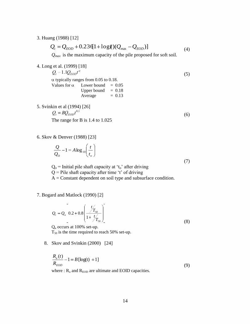
3. Huang (1988) [12]

(4)

Qmax is the maximum capacity of the pile proposed for soft soil.

4. Long et al. (1999) [18]

Qt 1.1QEODt (5)

typically ranges from 0.05 to 0.18.

Values for Lower bound = 0.05

Upper bound = 0.18

Average = 0.13

5. Svinkin et al (1994) [26]

Qt BQEODt0.1

(6)

The range for B is 1.4 to 1.025

6. Skov & Denver (1988) [23]

(7)

Qo = Initial pile shaft capacity at „to‟ after driving

Q = Pile shaft capacity after time „t‟ of driving

A = Constant dependent on soil type and subsurface condition.

7. Bogard and Matlock (1990) [2]

50

50

1 8.02.0

Tt

Tt

QQ ut

(8)

Qu occurs at 100% set-up.

T50 is the time required to reach 50% set-up.

8. Skov and Svinkin (2000) [24]

1][log(t) 1)(

BR

tR

EOD

u

(9)

where : Ru and REOD are ultimate and EOID capacities.

)])(log(1[236.0 max EODEODt QQtQQ

oO t

tA

Q

Q10log1

15

Analysis of Set-up Behavior

The set-up data of twenty three piles was compiled along with time, pile length,

pile diameter. The liquid limit, plastic limit, average clay and silt content, average SPT

value were compiled along the pile length. The length and diameter of the piles varied

from site to site.

Soil Characteristics

From the compiled data, it was observed that the piles were primarily in clay-silt

mixed soils. The average clay and silt contents of the soil along the length of the piles

are shown in figure 1-A. It can be seen that the soils were primarily a mixture of clay and

silt and that the silt fraction was larger than the clay fraction in most cases. Clay and silt

content data was not available for piles 5 and 6. The average values of the liquid limit and

plasticity index are shown in figures 1-B and 1-C. Soils along piles 1,8,9,21 and 22 were

non-plastic (NP). The LL ranged from 15 to 30 and the PI ranged from 5 to 16. Figure 1-

D shows the average SPT values along the pile length. The range was from 6 to 24.

Figure 1-A: Average clay and silt content in soil within the pile embedment.

0

10

20

30

40

50

60

70

80

90

100

1 2 3 4 5 6 7 8 9 10 11 12 13 14 15 16 17 18 19 20 21 22 23

Pe

rce

nt

Pile number

Avg. Silt content

Avg. Clay content

16

Figure 1- B: Average Liquid limit of soil within the pile embedment.

Figure 1- C: Average Plasticity Index (PI) of soil within the pile embedment.

Figure 1-D: Average SPT value of soil within the pile embedment.

0

5

10

15

20

25

30

35

1 2 3 4 5 6 7 8 9 1011121314151617181920212223

Ave

rage

Liq

uid

Lim

it (

LL)

Pile number

0

2

4

6

8

10

12

14

16

18

1 2 3 4 5 6 7 8 9 10 11 12 13 14 15 16 17 18 19 20 21 22 23

Pla

stic

ity

Ind

ex

(PI)

Pile number

0

5

10

15

20

25

30

1 2 3 4 5 6 7 8 9 10 11 12 13 14 15 16 17 18 19 20 21 22 23Avg

. N v

alu

e a

lon

g th

e p

ile le

ngt

h

Pile number

17

EOID and Restrike Capacities

Figure 2-A shows the comparison of total capacities of the piles before and after

restrike. A total of 23 pile data were compiled. In terms of total capacities, 21 piles

showed set up and 2 piles (pile 16 and 17) experienced relaxation. Figure 2-B shows

the shaft capacities before and after restrikes. The data indicated that the shaft capacities

had increased in case of all the 23 piles. A comparison of the tip capacities (figure 2-C)

indicated that in several (piles 1,5,16 and 17) instances, the tip capacities were observed

to have decreased from the EOID values. A possible reason for this is that the shaft

friction had increased to a point such that less energy from the hammer was getting

transferred to the pile toe. The tip capacity estimation by the dynamic methods is limited

by the amount of energy that reaches the pile tip.

The restrike times of the piles varied from about 1.5 hours to about 170 hours.

For reference purpose, the length variation of the twenty three piles are shown in figure

2-D. The length of the piles varied from 15 ft. to 131 ft.

Figure 2-A: Comparison of initial and restrike total and shaft capacities

0

100

200

300

400

500

600

1 2 3 4 5 6 7 8 9 10 11 12 13 14 15 16 17 18 19 20 21 22 23

Pile

Lo

ad (

Kip

)

Pile number

Intial Capacity Total (kips)

Restrike Capacity Total (kips)

18

Figure 2-B: Comparison of initial and restrike shaft capacities.

Figure 2-C: Comparison of initial and final tip capacities.

0

50

100

150

200

250

300

350

400

450

1 2 3 4 5 6 7 8 9 10 11 12 13 14 15 16 17 18 19 20 21 22 23

Pile

Lo

ad (

Kip

)

Pile number

Intial Shaft capacity (kips)

Restrike Capacity Shaft (kips)

0

50

100

150

200

250

300

350

400

450

1 2 3 4 5 6 7 8 9 10 11 12 13 14 15 16 17 18 19 20 21 22 23

Pile

Lo

ad (

Kip

)

Pile number

Tip Capacity Initial

Tip Capacity Restrike

19

Figure 2-D: Length of the twenty three piles investigated.

Set-up evaluation criteria

The pile set-up equations are generally applicable to the same pile or identical

piles driven into identical soil strata. In this study, the piles were driven into soil profiles

with variable characteristics, and the length and diameter varied from site to site.

Therefore, it was not unexpected that the set-up data would be scattered. The

investigation focused on identifying any trend or correlation that would allow ODOT to

estimate set-up in future projects.

The compiled data indicated that some piles were above the water table while

others were primarily submerged under the water table. For the purpose of analysis, the

piles were divided into three groups based on submergence: G-1 (piles above water

table), G-2 (piles with less than 50% submergence) and G-3 (piles with greater than 89 %

submergence) to identify the effect of water table. As mentioned previously, most of the

piles were in mixed clay-silt layers. The A value of the Skov & Denver equation [23] has

been reported to give good correlations for set-up and was chosen in this research to

evaluate the set-up characteristics of the driven piles. Since many of the pile restrikes

were carried out in less than 24 hour time, the value of to was chosen to be one hour (to

= 1 hr.).

The computed A values are shown in figure 3. A large scatter was observed

which ranged from 0.08 to 3.16.

0

20

40

60

80

100

120

140

1 2 3 4 5 6 7 8 9 10 11 12 13 14 15 16 17 18 19 20 21 22 23

Pile

Le

ngt

h (

ft)

Pile number

20

Figure 3: Skov-Denver „A’ values for steel pipe piles based on initial and restrike shaft capacities.

Effect of length

The variation of the calculated A values with the pile length are shown in figure 4.

The values were scattered and did not show any correlation. However, an increasing

trend of the A value was observed with increasing pile length for groups G-2 and G-3.

Figure 4: Variation of A value with pile length.

The A values were also plotted against the L/D ratios (figure 5). The increasing trend of

the A values was again observed in this plot for the G-2 and G-3 piles. The data points

were scattered.

0.00

0.50

1.00

1.50

2.00

2.50

3.00

3.50

1 2 3 4 5 6 7 8 9 10 11 12 13 14 15 16 17 18 19 20 21 22 23

Sko

v &

Den

ver

A v

alu

e

Pile number

0

0.5

1

1.5

2

2.5

0 50 100 150

'A'

Pile length (ft)

Above WT

<50% submerged

>89% submerged

21

Figure 5: Variation of A value with L/D ratio of piles.

The variation of A was also plotted against LD and LD

2 of the piles (figures 6-A

and 6-B). Dependence of A on LD would indicate that the pile surface area influences

set-up, while dependence on LD2 would indicate that the displaced volume during pile

driving influences set-up. However, no correlation was observed in either case. An

increasing trend of A was observed for G-3 piles when plotted against LD. However,

this trend was no longer observed in case A vs. LD2 plot.

Figure 6-A: Variation of A values with LD values of piles.

0

0.5

1

1.5

2

2.5

0 20 40 60 80 100 120

'A'

L/D

Above WT

<50% submerged

>89% submerged

0.77

0

0.5

1

1.5

2

2.5

0 50 100 150 200

'A'

LD

Above WT

<50% sub

>89% sub

22

Figure 6-B: Variation of A value with LD

2 of piles.

The A values were plotted against the time of restrike to investigate any possible

correlation (figure 7). As seen in the figure, the time of restrike of the three groups were

random. The data had a large scatter and did not show any trend, except for the G-2

piles, which showed a decreasing trend of the A values with time. However, the data

points were too few to give any meaningful correlation.

Figure 7: Variation of A value with time of restrike of piles.

Effect of clay and silt content

As noted earlier, all the piles were in mixed clay – silt soils. The variation of the

computed A values with the average liquid limit and clay activity (PI / % clay) are shown

in figures 8 and 9. The data was scattered for the three groups in both cases. It appears

0

0.5

1

1.5

2

2.5

0 50 100 150 200 250

'A'

LD2

Above WT

>50% sub

>89% sub

0

0.5

1

1.5

2

2.5

0 50 100 150 200

'A'

Time (hr)

Above WT

<50% sub

> 89% sub

23

that the LL and clay activity did not have any correlation to the observed set-up. The

variation of the A value with the silt content is shown in figure 10. The data showed a

very large scatter. It should be kept in mind that LL, PL, clay and silt contents are

average values along the pile shaft.

Figure 8: Variation of A with the average LL of the soil.

Figure 9: Variation of A with the average Clay Activity of the soil.

0

0.5

1

1.5

2

2.5

0 10 20 30 40

'A'

LL

Above WT

<50% sub

>89% sub

0

0.5

1

1.5

2

2.5

0 0.1 0.2 0.3 0.4 0.5 0.6 0.7 0.8

'A'

Clay activity

Above WT

<50% sub

>80% sub

24

Figure 10: Variation of A with the average silt content of the soil.

Effect of Standard Penetration Test (SPT) value

The variation of A values with average SPT numbers along the pile length is

shown in figure 11. Again, the data was widely scattered and no trend was observed.

Figure 11: Variation of A with the average SPT value along the pile length.

0

0.5

1

1.5

2

2.5

0 10 20 30 40 50 60

'A'

Silt content (%)

Above WT

<50% sub

>89% sub

0

0.5

1

1.5

2

2.5

0 5 10 15 20 25 30

'A'

Average SPT value

Above WT

<50% sub

>80% sub

25

The variation of the normalized pile shaft capacity increase was investigated in

terms of restrike time. The data was scattered and no correlation was observed (figure

12).

Figure 12: Variation of normalized pile shaft capacity with time.

Effect of Restrike Time on Set-up rate

The Skov & Denver „A‟ values from different sites could not be correlated. The

possibility of a power correlation was then investigated. For this purpose, the rate of

strength gain ( (Q/Qo)/t) was plotted against restrike time. The variation was investigated

for both total (figure 13) and shaft (figure 14) capacities of the piles. The piles that

showed relaxation in terms of total capacity were excluded while plotting data points in

figure 13.

In both cases, very good correlations were obtained. The best-fit regression

curves along with the regression equations for each case, are also shown in figures 13 and

14. When the total pile capacities were considered, a very strong correlation with R2

=

0.9732 was obtained. When the shaft capacities were considered, the correlation was also

very good with R2= 0.8817, but less strong than of the total capacity correlation. It

should be noted that all twenty three piles showed strength gain during restrike in terms

of shaft capacity and therefore figure 14 includes capacity of all the piles investigated.

No significant change in correlation was observed when the data of piles that experienced

overall relaxation was excluded from this plot.

0.00

0.01

0.02

0.03

0.04

0.05

0.06

0.07

0 50 100 150 200

(Q-Q

o)/

Qo

LD

Restrike time (hr)

26

Figure 13: Variation of rate of pile strength gain in terms of total capacity, with time of restrike.

Figure 14: Variation of rate of pile strength gain in terms of shaft capacity, with time of restrike.

y = 0.9957x-0.913

R² = 0.9732

0.00

0.10

0.20

0.30

0.40

0.50

0.60

0.70

0.80

0.90

1 10 100 1000

(Q/Q

o)/

t

Time (hr)

y = 1.3005x-0.889

R² = 0.8817

0.00

0.20

0.40

0.60

0.80

1.00

1.20

1 10 100 1000

(Q/Q

o)/

t

Time (hr)

27

Predicting Pile Set-up

Several combinations of the known parameters were investigated for establishing

correlations between the pile set-up and the measured field values. At the end, only the

correlation obtained in figure 13 seemed meaningful, and was considered further.

Revisiting the strong correlation between [Q/Qo]/t vs. t obtained for the total pile

capacities (figure 13), the following regression equation is considered.

913.09957.0 xy (10)

where y = [Q/Qo]/t

x = time is set-up in hours.

Substituting the value of y and rearranging the terms, the following equation for

calculating pile set-up is obtained.

087..09957.0 tQQ o (11)

where: Q is the pile capacity (kip) after time t ,

Qo is the EOID pile capacity (kip),

t is the time in hours.

It may be noted here that equation (11) has the same form as the set-up equations

proposed by Long [18], Svinkin [25, 26]. However, the coefficients obtained for Ohio

soils were slightly different than the values proposed in those references.

To verify the applicability of equation (11), Q values were calculated with the

known Qo and t values of the twenty one piles where set-up had occurred. The calculated

values of Q were plotted along with the actual (restrike) Q values against the initial

capacities Qo, as shown in figure 15. The values were calculated with the coefficient 0.9

instead of 0.9957 and showed slightly more agreement in case of high (> 400 kip) Qo

values.

Figure 15: Comparison of restrike total capacity with the calculated pile capacities plotted

against the EOID values. .

0

100

200

300

400

500

600

700

0 100 200 300 400 500 600

Tota

l res

trik

e ca

pac

ity

Q

(kip

)

Total EOD pile capacity Qo (kip)

Q (calculated)

Q (restrike)

28

Figure 16: Comparison of restrike and calculated pile capacities.

It is evident that the proposed equation (11) predicted the pile set-up at different

ODOT sites with reasonable accuracy even though the site conditions were different.

The implication of this result is that the proposed equation has universal

applicability to all the investigated sites where set-up had occurred, and therefore,

may be used for predicting set-up of small diameter driven steel pipe piles in Ohio

soils. However, it is advisable to test the correlation with another group of pile set-up data,

preferably from static load tests.

Implementation

A correlation has been established between the EOID capacity of the piles and the

strength gain with time. In order to develop an implementation method, the time

dependent strength gains of two arbitrarily chosen piles, Pile-12 and Pile-14, were

calculated using equation (11) and plotted in figure 17. It can be seen that the piles

would gain most of its strength by 30 days.

For the purpose of design, conservatively the 30 day strength may be assumed as

the capacity of the pile (Q). Using this Q value, the EOID capacity (Qo) of the pile

expected in the field can be calculated from equation (11). In order to translate the Qo

value to pile dimensions L and D, a correlation is required among them.

0

100

200

300

400

500

600

700

800

900

1000

1 2 3 4 5 6 7 8 9 10 11 12 13 14 15 16 17 18 19 20 21 22 23

Pile

Cap

acit

y Q

(ki

p)

Pile Number

Q (calculated)

Q (restrike)

29

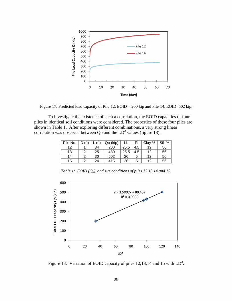
Figure 17: Predicted load capacity of Pile-12, EOID = 200 kip and Pile-14, EOID=502 kip.

To investigate the existence of such a correlation, the EOID capacities of four

piles in identical soil conditions were considered. The properties of these four piles are

shown in Table 1. After exploring different combinations, a very strong linear

correlation was observed between Qo and the LD2 values (figure 18).

Pile No. D (ft) L (ft) Qo (kip) LL PI Clay % Silt %

12 1 34 200 25.5 4.5 12 56

13 2 25 430 25.5 4.5 12 56

14 2 30 502 26 5 12 56

15 2 24 415 26 5 12 56

Table 1: EOID (Qo) and site conditions of piles 12,13,14 and 15.

Figure 18: Variation of EOID capacity of piles 12,13,14 and 15 with LD

2.

0

100

200

300

400

500

600

700

800

900

1000

0 10 20 30 40 50 60 70

Pile

Lo

ad C

apac

ity

Q (

kip

)

Time (day)

Pile 12

Pile 14

y = 3.5007x + 80.437R² = 0.9999

0

100

200

300

400

500

600

0 20 40 60 80 100 120 140

Tota

l EO

ID C

apac

ity

Qo

(ki

p)

LD2

30

The intercept of the correlation equation shown in figure 18, in theory, should be

zero. However the correlation simply indicates that the relationship above a certain

critical value of LD2 is linear. Further research is necessary to verify this correlation and

establish the critical value of LD2.

It is conceivable that such a linear relationship would exist between Qo and LD2 at

other Ohio sites also. A general linear equation is therefore proposed to correlate EOID

capacities of preconstruction test piles and design piles.

Qo = K1 LD

2 + K2 (12)

Where, Qo = EOID capacity

L = pile length

D = pile diameter

K1, K2 = site specific constants

The constants K1 and K2 can be evaluated from two EIOD values of a preconstruction test

pile measured at two different embedment lengths.

Pile Design

Based on discussions presented in the previous sections, the design of small

diameter driven steel pipe piles in Ohio soils is proposed as follows. The proposed

method requires driving of a preconstruction test pile at the site, and determination of

EOID capacities at two different embedment lengths L1 and L2, which could be

substantially shorter than the expected design lengths. Measurement of restrike capacity

is also required to ensure occurrence of set-up.

Design Steps:

1. Determine the required design load capacity Q of the pile.

2. Using equation (11), determine the required EOID, i.e. Qo (required) in the field for a

desired pile capacity Q. Use time t as 30 days (arbitrarily set).

3. Choose a pile diameter D.

4. Determine the constants K1 and K2 for equation (12) from EOID capacities of the

preconstruction test pile of diameter D and embedment lengths L1and L2.

5. Using the constants evaluated in step-3, along with D and Qo (required), determine

the design pile length L from equation (12).

6. Use an appropriate FS to increase the length.

31

Site Characterization

The set-up of twenty three piles could not be correlated to the soil parameters

measured at the ODOT sites. Therefore no specific test could be suggested to identify

pile set-up. Torque measurement may be considered at the pile installation sites along

with SPT. It has been reported in the literature that the combination of torque and SPT

could provide set-up information [4]. Also, since the sites have predominantly fine

grained soils, Cone Penetration Tests (CPT) could provide useful data for set-up analysis.

Further research is required in this area.

Conclusions

The following conclusions were drawn from the analysis.

The subsurface soil along the pile shafts at sites investigated were predominantly

clay - silt mixtures, with larger silt fractions in most cases.

Set-up occurred commonly in driven steel piles in Ohio soils. In 91% cases some

degree of set-up was observed.

Relaxation of piles occurred rarely. In about 9% cases relaxation was observed.

The set-up primarily occurred at the pile shafts.

The Skov & Denver „A‟ parameter varied from 0.08 to 3.16 for the piles

investigated. This equation was not applicable for set-up prediction of piles

investigated.

Pile set-up in general showed an increasing trend with increasing pile lengths.

However, the data was too scattered for any meaningful correlation.

There was no correlation between the „A‟ values and the average clay content,

LL,PI or clay activity along the pile shaft.

No correlation was observed for „A‟ values with the average silt content along the

pile shaft.

No set-up correlation was observed with the average SPT values along the pile

shaft.

No correlation was observed between the normalized shaft capacity increase and

the restrike time.

Effect of pile submergence on set-up not distinguishable.

Strong correlations were observed between (Q/Qo)/t vs. t in terms of total and

shaft capacities. The correlation for the total pile capacities was stronger than the

shaft capacities.

An equation for pile set-up in Ohio soils was developed for driven steel pipe piles,

and shown to be applicable universally to all ODOT sites investigated.

The EOID capacity of driven steel pipe piles under identical site conditions was

shown to vary linearly with LD2. However, additional research is required for

further verification of this correlation.

Based on the correlations developed, a design method for small diameter driven

steel pipe piles has been proposed for the implementation of the research findings.

32

Acknowledgements Mr. Peter Narsavage provided the bulk of the ODOT pile setup data that were analyzed

in this project. Dr. Bashr Altarawneh also provide set-up data for the research. Additional

important pile set-up data was provided by Dr. Frank Rausche of GRL. The authors are grateful

to all for their valuable assistance and input which made this research possible. The authors are

also indebted to Dr. Jawdat Siddiqi for his valuable inputs and to Ms. Vicky Fout for

coordinating the project.

REFERENCES

1) Attwooll WJ, Holloway MD, Rollins KM, Esrig MI, Si S, Hemenway D. (1999). “Measured

Pile Setup during Load Testing and Production Piling: I-15 Corridor Reconstruction Project

in Salt Lake City, Utah.” Transportation Research Record 1663, Paper No.99-1140, pp. 1-7.

2) Bogard, J.D., Matlock, H. . “Application of Model Pile Tests to Axial Pile Design.”

Proceedings of the 22nd

Annual Offshore Technology Conference, May 1990. Tex. 7-10 Vol.

3, pp. 271-278.

3) Bullock, PJ. “A Study of the Setup Behavior of Drilled Shafts.” Florida Department of

Transportation, July 2003.

4) Bullock, PJ, Schmertmann JH, McVay MC, Townsend FC. (2005). “Side Shear Setup.I: Test

Piles Driven in Florida.” Journal of Geotechnical and Geoenvironmental Engineering, March

2005.

5) Bullock PJ, Schmertmann JH, McVay MC, Townsend FC. (2005). “Side Shear Setup.II: Test

Piles Driven in Florida.” Journal of Geotechnical and Geoenvironmental Engineering, March

2005.

6) Chow FC, Jardine RJ, Nauroy JF, Brucy F. (1997). “Time-related Increase in Shaft

Capacities of Driven Piles in Sand.” Géotechnique, Vol. 47, No. 2, pp. 353-361.

7) Elias, M. “Numerical Simulation of Pile Installation and Set-up.” Diss. U. of Wisconsin-

Milwaukee 2008.

8) Fellenius, Bengt H, Riker RE, O‟Brien AJ, and Tracy GR. (1989). “Dynamic and Static

Testing in Soil Exhibiting Set-Up.” Journal of Geotechnical Engineering, Volume 115, No.

7, ASCE, pp. 984-1001.

33

9) Fellenius BH, Harris DE, Anderson DG. (2004) “Static loading test on a 45 m long pipe pile

in Sandpoint, Idaho.” Can. Geotech. J. 41: 613-628.

10) Guang-Yu, Z. (1988). “Wave Equation Applications for Piles in Soft Ground.” Proceedings

3rd

International Conference on the Application of Stress-Wave Theory to Piles, Ottawa,

Ontario, Canada, pp. 831-836.

11) Horsfall, J. “Bridge Piles: More Capacity Over Time?” Wisconsin Department of

Transportation, September 2003.

12) Huang, S. (1988) “Application of Dynamic Measurement on Long H-Pile Driven into Soft

Ground in Shanghai.” Proceedings 3rd

International Conference on the Application of Stress-

Wave Theory to Piles, Ottawa, Ontario, Canada, pp. 635-643.

13) Hussein M, Likins G. (1995). “Dynamic Testing of Pile foundations during Construction.”

Proceedings of Structures Congress XIII Structural Division: ASCE, pp 1349-1364.

14) Hussein M, Mondello B, Alvarez C. “Simulated Pile Load-Movement Incorporation

Anticipated Soil Set-up.” Geotechnical Engineering for Transportation Projects pp. 1153-

1160.

15) Komurka VE. (2004).”Incorporation Set-up and Support Cost Distributions into Driven Pile

Design.” Current Practices and Future Trends in Deep Foundations, pp 16-49.

16) Komurka, VE. “Incorporating Set-up Into Driven Pile Design and Installation.” pp. 13-20.

17) Long J, Bozkurt H, Diyar, Kerrigan JA, and Wysockey MH. (1999). “Value of Methods for

Predicting Axial Pile Capacity.” Transportation Research Record 1663, Paper No. 99-1333,

pp. 57-63.

18) Long JH, Kerrigan JA, Wysockey MH. (1999). “Measured Time Effects for Axial Capacity

of Driven Piling.” Transportation Research Record 1663, Paper No. 99-1183, pp.8-15.

19) Randolph MF, Carter JP, Wroth CP. (1979). “Driven Piles in Clay – The Effects of

Installation and Subsequent Consolidation.” Géotechnique 29, No. 4, pp. 361-393.

20) Rausche F, Goble GG, Likins GE. (1985). “Dynamic Determination of Pile Capacity.”

Journal of Geotechnical Engineering, Volume 111, No. 3, ASCE, pp. 367-383.

21) Rausche F, Robinson B, Likins G. August, 2004. “On the Prediction of Long Term Pile

Capacity from End-of-Driving Information,” Current Practices and Future Trends in Deep

Foundations, Geotechnical Special Publication No. 125.

22) Skov R, Svinkin (2009) “Set-Up Effect of Cohesive Soils in Pile Capacity.”

Vulcanhammer.Net, www.vulcanhammer.net/svinkin/set.php

23) Skov R, Denver H. (1988). “Time-Dependence of Bearing Capacity of Piles.” Proceedings

3rd International Conference on Application of Stress-Waves to Piles, pp. 1-10.

24) Skov R, Svinkin, Mark R. (2000). “Set-Up Effect of Cohesive Soils in Pile Capacity.” Proceedings 6

th International Conference on Application of Stress

34

Waves to Piles, pp. 107-111.

25) Svinkin, M.R., “Discussion on Setup and Relaxation in Glacial Sand.” Journal of

Geotechnical Enigneering, ASCE, Vol. 122, April 1996, pp. 319-321.

26) Svinkin, M.R., Morgano, C.M., Morvant, M. “Pile Capacity as a Function of Time in Clayey

and Sandy Soils.” Proceedings of the 5th International Conference and Exhibition on Piling

and Deep Foundations, June 1994. Deep Foundations Institute, pp. 1.11.1-1.11.8.

27) Titi HH, Wathugala G,Wije, (1999). “Numerical Procedure for Predicting Pile Capacity –

Setup/Freeze.” Transportation Research Record 1663, Paper No.99-0942, pp. 25-32.

28) Titi, H,. “Increase in Shaft Capacity with Time for Friction Piles Driven Into Saturated Clay.”

ProQuest Cleveland State University Lib., Cleveland, OH July 2009.

29) Whittle AJ, Sutabutr T. (1999). “Prediction of Pile Setup in Clay” Transportation Research

Record 1663, Paper No.99-1152, pp. 33-40.

30) Yang L, Liang R. (2009). “Incorporating Set-up into Load and Resistance Factor Design of

Driven Piles in Sand.” Can. Geotech. J. 46: pg. 296—305.