prediction of dynamic groundwater levels using an ... · first international colloquium rezas12...

First International Colloquium REZAS12Morocco, 14-16 November, 2012

MSc. Hasan SirhanGeohydraulic and Engineering Hydrology 1

AuthorsHasan Sirhan* and Manfred Koch*

* Department of Geohydraulics and Engineering Hydrology,Faculty of Civil and Environmental Engineering

Kassel University, Germany

Prediction of Dynamic Groundwater Levels Using an Artificial Neural

Network (ANN) Approach in the Gaza Coastal Aquifer, South Palestine

First International Colloquium REZAS12: " Water resources in the arid and semi-arid regions-challenges and prospects. Case of the African continent"

Beni Mellal, Morocco, November 14-16, 2012



Content:

• Natural Neural Network

• Definition of Artificial Neural Network

• Why Artificial Neural Network

• ANN Properties

• Artificial Neural Networks Learning

• Development of ANN model for prediction of groundwater levels.

What is a Neural Network?



The Neural Network of the human brain can:

• Collect more than 10 billion interconnected “neurons”.

• Transmit information and computes some function (biochemical reactions).

• Takes input as treelike network dendrites.

• Produces (output) and connected to each other by synapses (weights).

• Can learn and makes appropriate decisions.



What is an Artificial Neural Network (ANN)?

• The first studies on Artificial Neural Networks (ANNs) were prompted based on

computers mimic human learning and created in (1943).

• Artificial neural networks are a simplified mathematical model of a natural neural

network inspired by biological nervous of the brain.

• A Computing system which can be model based on the simple quantifiable and highly

interconnected input variables.



Why Artificial Neural Network?

• ANN’s are a relatively new approach for groundwater levels modeling and an

attractive tool for traditional physical-based numerical models.

• It is not necessary to characterize and quantify the physical properties in explicit way

as in the numerical models.

• The system can be model based on the simple quantifiable input variables.



An artificial neural network is a model of reasoning based on the analogy with the human brain.

Biological Neural Network Artificial Neural NetworkSoma Neuron Dendrite Input (receptive zones)Axon Output

Synapse (mediate the interactions between neurons)

Weight

Analogy between biological and artificial neural networks



ANNs Properties

• Inputs are flexible

� Any real values

� Highly correlated or independent

• Fast evaluation and less time consumed compared to the traditional (numeric) models.

• In training process, it is highly important to deal with consistent data set of patterns.

• The neural network model act as a black box, therefore the function produced can be

difficult for humans to interpret.



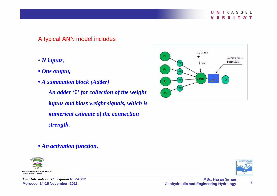
A typical ANN model includes

• N inputs,

• One output,

• A summation block (Adder)

An adder ‘Σ’ for collection of the weight

inputs and biass weight signals, which is

numerical estimate of the connection

strength.

• An activation function.



Approach

• The activation values of the input nodes are weighted and accumulated at each node

in the first layer.

• The weighted input nodes are transformed by an activation function into the node’s

activation value.

• Take output from first layer neurons as input to the next layer, until eventually the

output activation values are found.

The neuron output O is given by the following relationship:

Where

• Wj is the input connection weight,

• Pi is the input,

• X0 is the biass (not an input) and

• W0 is the biass weight.

O = f (net) = f ��∑ �� = + � � ��



Activation function

• The activation function determines the relationship between inputs and outputs of a node and a network.

Sigmoid (logistic) function hyperbolic tangent(tanh) function

linear function

Among them, logistic transfer function is the most popular choice. It has a

nature nonlinearity and it can be used for both hidden and output nodes.



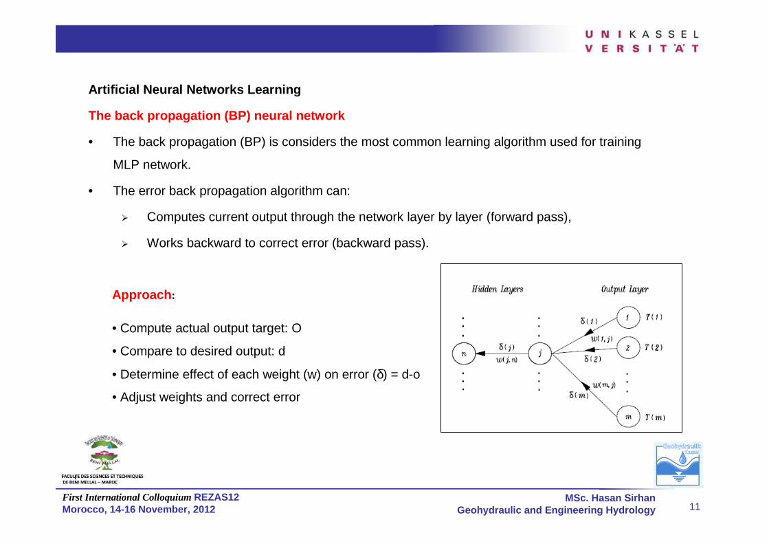
Artificial Neural Networks Learning

The back propagation (BP) neural network

• The back propagation (BP) is considers the most common learning algorithm used for training

MLP network.

• The error back propagation algorithm can:

� Computes current output through the network layer by layer (forward pass),

� Works backward to correct error (backward pass).

Approach:

• Compute actual output target: O

• Compare to desired output: d

• Determine effect of each weight (w) on error (δ) = d-o

• Adjust weights and correct error



Application of Artificial Neural Network

• Application in hydrology

An approximation of any continuous (non-linear) relationship can be carried out.

• Application in groundwater

Ground water levels predicting can be applied under variable weather conditions

and under pumping conditions.



The Study Area



The Study AreaGaza Strip

Geography

Palestine is composed of two-separated

areas, the Gaza strip and the West Bank.

The Gaza Strip is a very small area

located at the eastern coast of the

Mediterranean sea in the southwest of

Palestine.

Its length 40 km while its width varies

between 6 km in the north to 12 km in

the south, with an avg. area of 365Km2.



Development of ANN model

• The objective of the ANN model is to investigate the effects of the hydrological,

meteorological and human factors on the dynamic groundwater levels in the Gaza

coastal aquifer.

The ANN model can generalize a relationship between the output and input variables

having the form of:

Y = f (Xn)

where,

Xn is an n-dimensional input independents

including variables x1, x2, . . . , xn; and

Y is an output dependent variable.

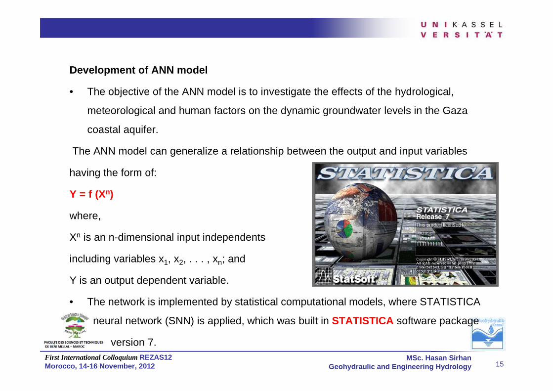
• The network is implemented by statistical computational models, where STATISTICA

neural network (SNN) is applied, which was built in STATISTICA software package

version 7.



Distribution of the study wells in the Gaza Strip

Independent input variables

� A 770 combination cases were extracted

from 70 study wells.

�These data were created from groundwater

time series data recorded between years 2000

and 2010.



Independent input variables, Cont.

In this study ANN were developed to predict average groundwater levels with

Seven predictors as input variables, namely:

• Initial ground water level,

• Recharge from rainfall,

• Distance of the study wells from the shore line,

• Depth to well screen from surface and

• The wells density for each governorate area in the Gaza strip.

The ANN model input variables can be represented in equation as follows:

WLf = f (WLi, Q, R, K, Ds-shore, Depth to scr., Well-density)

• Ground water extraction,

• Hydraulic conductivity,



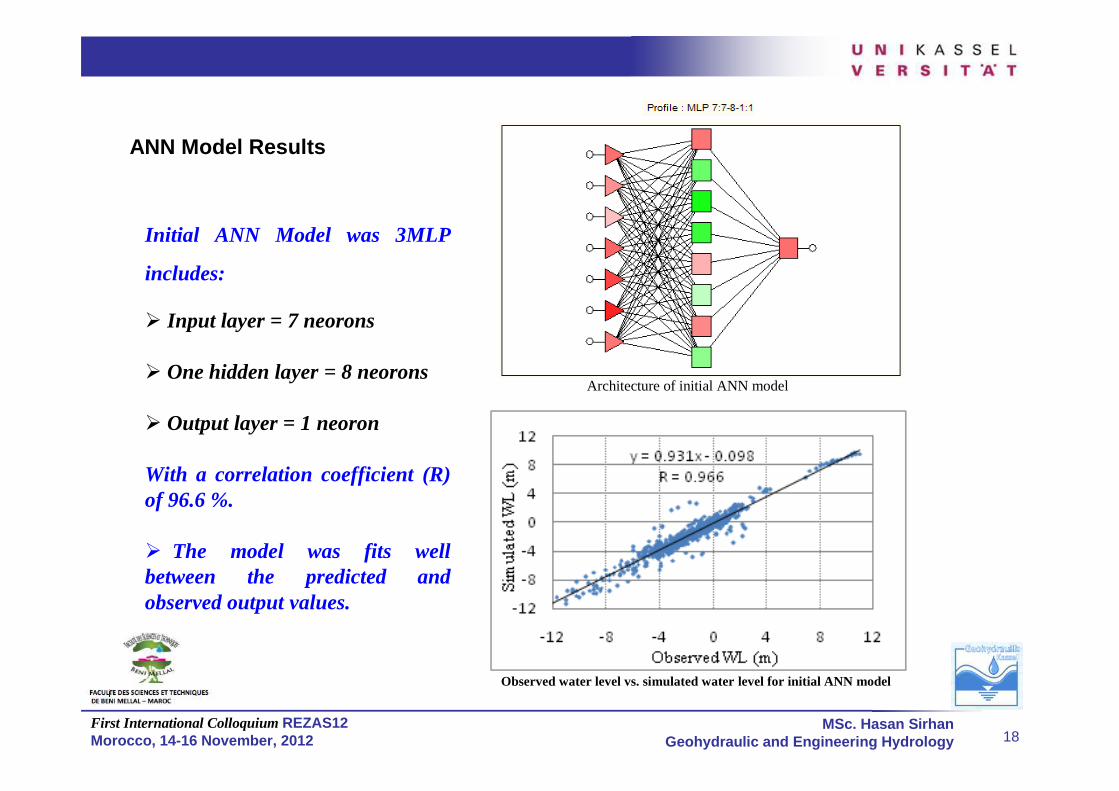
ANN Model Results

Architecture of initial ANN model

Observed water level vs. simulated water level for initial ANN model

Initial ANN Model was 3MLP

includes:

� Input layer = 7 neorons

� One hidden layer = 8 neorons

� Output layer = 1 neoron

With a correlation coefficient (R) of 96.6 %.

� The model was fits well between the predicted and observed output values.



Sensitivity Analysis

A sensitivity analysis has been demonstrated to:

• Describe how much model output values are affected by changes in model

input values.

• Give a strong confirmation for the usefulness and the un-influential individual input variables.

• The basic sensitivity figure is the error ratio, for each variable, the network is

executed as if that variable is unavailable (excluded).

Sensitivity analysis results

• Both the independent variables of depth to well screen and hydraulic

conductivity are the most un-influential variables affecting groundwater levels

due having a small error ratio.



Final ANN Model

Based on the results derived from sensitivity analysis, the final neural network models

were formatted using all the retained five input variables (neurons) namely,

• Initial water level (WLo),

• Abstraction (Q),

• Recharge rate,

• Distance from sea shore line (Ds), and

• Well density (W-density).

The attained network was (4MLP), with:

• An input layer of 5 neurons • A second hidden layer with 20 neurons

• A sigmoid activation function in between the layers.

Architecture of initial ANN model

• A first hidden layer with 30 neurons• One output layer with one neuron



The attained model results indicate that the model was fits well between the predicted and observed output values showing a correlation coefficient (R) of

96.9 %.

Observed water level vs. simulated water level for final ANN model

Simulated water level vs. the Observed water level on year 2000.



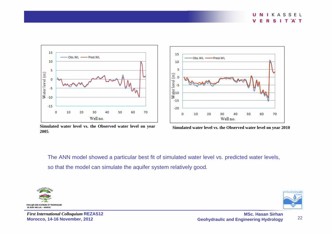
Simulated water level vs. the Observed water level on year 2005.

Simulated water level vs. the Observed water level on year 2010

The ANN model showed a particular best fit of simulated water level vs. predicted water levels,

so that the model can simulate the aquifer system relatively good.



Response Graph

Represents a relationship

between the independent

variables and the output

dependent variable

individually by a number

of plateaus.



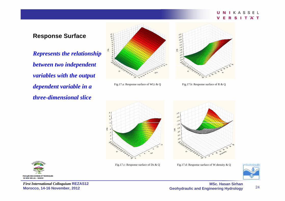
Fig.17.a: Response surface of WLi & Q

Fig.17.b: Response surface of R & Q

Fig.17.c: Response surface of Ds & Q

Fig.17.d: Response surface of W-density & Q

Response Surface

Represents the relationship

between two independent

variables with the output

dependent variable in a

three-dimensional slice



Conclusion

� The attained optimal network model was fits well between the predicted and observed

output values of water levels showing an overall correlation coefficient (R) of 96.9 %.

The attained model represented a reasonably non-linear relationship between:

� The individual independent variable and dependent variable as showed in the

response graph.

�A two independent variables with the output dependent variable relationship in a three-

dimension as showed in the response surface.

The results indicated that the model simulation represents the behavior of the aquifer quite

well under the existing conditions of the influencing independent variables.



End

Thank you

prediction of dynamic groundwater levels using an ... · first international colloquium rezas12...

Documents