PREDICTING WATER USE, CROP GROWTH AND QUALITY OF BERMUDA GRASS UNDER SALINE

IRRIGATION

FINAL REPORT TO THE

CALIFORNIA DEPARTMENT OF WATER RESOURCES

CONTRACT #: 4600004616

Prepared by

Maximo F. Alonso and Stephen R. Kaffka

University of California, Davis

October 15th, 2009

2

Principal investigators Stephen Kaffka, Department of Plant Sciences, Mail Stop 1, University of California, One Shields Ave. Davis, CA 95616-8750, Tel: 530-752-9108, srkaffka@ucdavis.edu. Steve Grattan, Department of Land, Air and Water Resources, University of California, Davis, Tel: 530-752-4618, srgrattan@ucdavis.edu Cooperators Dennis Corwin, George E. Brown Jr. Salinity Lab, USDA/ARS, 450 W. Big Springs Road, Riverside, CA, Tel: 951-369-4819, dcorwin@ussl.ars.usda.gov Maximo Alonso, Department of Plant Sciences, University of California, Davis, Tel: 530-752-4112, malonso@ucdavis.edu Blaine Hanson, Department of Land, Air and Water Resources, University of California, Davis, Tel: 530-752-4639, brhanson@ucdavis.edu Richard Snyder, Department of Land, Air and Water Resources, University of California, Davis, Tel: 530-7524628, rlsnyder@ucdavis.edu

3

TABLE OF CONTENTS

Summary ………………………………………………………………………………….... 4 INTRODUCTION …………………………………………………………………………. 5 PROJECT SPECIFIC TASKS ……………………………………………………………... 5 Quantification of Bermuda grass growth and quality under varying saline conditions and N fertilizer levels ……………………………………………………………………………………..

5

Bermuda grass Kc ………………………………………………..………………………….. 5 Bermuda grass yield …………………………………………………………………………. 6 Bermuda grass quality ………………………………………………………………………. 8 Grazing trials …………………………………………………………………………………. 13 Formulation of a simple model to predict Bermuda grass growth and quality as a function of water use, N fertility and soil salinity …………………………………………………………

14

The model ……………………………………………………………………………………… 14 Soil moisture …………………………………………………………………………... 14 Soil salinity …………………………………………………………………………….. 16 Soil trace minerals ……………………………………………………………………. 18 Plant yield and quality ……………………………………………………………….. 20 Grazing …………………………………………………………………………………. 21 Model validation ……………………………………………………………………………… 23 Forage production ……………………………………………………………………. 23 Beef cattle production ………………………………………………………………... 25 Final discussion ………………………………………………………………………………. 25 OTHER OUTPUTS OF THE PROJECT …………………………………………………... 26 Presentations …………………………………………………………………………………. 26 Publications …………………………………………………………………………………… 26 APPENDIX A: MODEL OPERATION GUIDE ……………………………………………... 27

4

Summary Reusing saline drainage and other waste waters to produce forages suitable for ruminant livestock production would help to alleviate the shortage of the forages needed for California’s expanding dairy herd and for beef and sheep production. It would also help to manage salinity problems in the western San Joaquin Valley (WSJV) providing an economic alternative to land retirement. In previous studies we have demonstrated that low quality drainage and waste waters can be used to produce forages on a salt-affected site in the WSJV while raising beef cattle without apparent adverse health effects and with acceptable rates of average daily gain. Our objectives for this study were: 1) to quantify the relationships between Bermuda grass growth and quality, soil and irrigation water salinity, and N fertilization level in saline soils; and 2) to create a simple model to predict grass growth and quality as a function of water use, N fertility and soil salinity. Our results indicate that Bermuda grass under an optimal irrigation with saline water (6 dS m-1) and fertilized with the equivalent to 600 kg N ha*y-1 can yield up to 20 ton DM ha*y-1 in a soil of 7 dS/m ECe. With a fertilization equivalent to 300 kg N ha*y-1 yields were close to 16 ton DM ha*y-1. Without fertilization yields were around 1 ton DM ha*y-1. Under grazing and a suboptimal irrigation Bermuda grass yields were between 5-7 ton DM ha*y-1. The leaf/stem ratio (LSR) was significantly different (p<0.05) between unfertilized and fertilized treatments. The difference between fertilized treatments (300 and 600 kg N ha*y-1) was not significant (p>0.05). The differences in LSR at different soil salinity levels (7, 14 and 22 dS/m) was not significant (p>0.05) also. Nitrogen fertilization not only increases yield, but changes the aerial composition of Bermuda grass. Our results indicate that nitrogen fertilization increases the proportion of leaves by 20% and decreases the proportion of inflorescences by the same percentage. The proportion of stems is not affected. Although the differences in the aerial composition between fertilized and unfertilized treatments were significant (p<0.05), they were not significant (p>0.05) between treatments fertilized with 300 and 600 kg N/ha. Differences in aerial composition between soil salinity levels were not significant (p>0.05). Model predictions fit observed values. Results of the model indicate the feasibility of growing Bermudagrass on the saline soils of the western San Joaquin Valley of California when irrigated with drainage water. Using crop-specific and site-specific parameters’ values the model could be used by farmers in the WSJV and elsewhere for salinity management and farm planning.

5

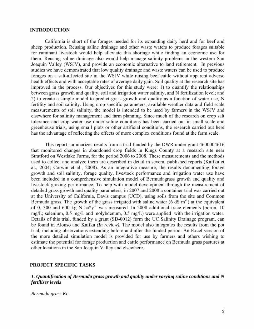
INTRODUCTION California is short of the forages needed for its expanding dairy herd and for beef and sheep production. Reusing saline drainage and other waste waters to produce forages suitable for ruminant livestock would help alleviate this shortage while finding an economic use for them. Reusing saline drainage also would help manage salinity problems in the western San Joaquin Valley (WSJV), and provide an economic alternative to land retirement. In previous studies we have demonstrated that low quality drainage and waste waters can be used to produce forages on a salt-affected site in the WSJV while raising beef cattle without apparent adverse health effects and with acceptable rates of average daily gain. Soil quality at the research site has improved in the process. Our objectives for this study were: 1) to quantify the relationships between grass growth and quality, soil and irrigation water salinity, and N fertilization level; and 2) to create a simple model to predict grass growth and quality as a function of water use, N fertility and soil salinity. Using crop-specific parameters, available weather data and field scale measurements of soil salinity, the model is intended to be used by farmers in the WSJV and elsewhere for salinity management and farm planning. Since much of the research on crop salt tolerance and crop water use under saline conditions has been carried out in small scale and greenhouse trials, using small plots or other artificial conditions, the research carried out here has the advantage of reflecting the effects of more complex conditions found at the farm scale. This report summarizes results from a trial funded by the DWR under grant 4600004616 that monitored changes in abandoned crop fields in Kings County at a research site near Stratford on Westlake Farms, for the period 2006 to 2008. These measurements and the methods used to collect and analyze them are described in detail in several published reports (Kaffka et al., 2004; Corwin et al., 2008). As an integrative measure, the results documenting forage growth and soil salinity, forage quality, livestock performance and irrigation water use have been included in a comprehensive simulation model of Bermudagrass growth and quality and livestock grazing performance. To help with model development through the measurement of detailed grass growth and quality parameters, in 2007 and 2008 a container trial was carried out at the University of California, Davis campus (UCD), using soils from the site and Common Bermuda grass. The growth of the grass irrigated with saline water (6 dS m-1) at the equivalent of 0, 300 and 600 kg N ha*y-1 was measured. In 2008 additional trace elements (boron, 10 mg/L; selenium, 0.5 mg/L and molybdenum, 0.5 mg/L) were applied with the irrigation water. Details of this trial, funded by a grant (SD-0012) form the UC Salinity Drainage program, can be found in Alonso and Kaffka (In review). The model also integrates the results from the pot trial, including observations extending before and after the funded period. An Excel version of the more detailed simulation model is provided for use by farmers and others wishing to estimate the potential for forage production and cattle performance on Bermuda grass pastures at other locations in the San Joaquin Valley and elsewhere. PROJECT SPECIFIC TASKS 1. Quantification of Bermuda grass growth and quality under varying saline conditions and N fertilizer levels Bermuda grass Kc

6

We quantified the relationships between Bermuda grass (Cynodon dactylon (L.) Pers.) used for pasture and hydrological, edaphic and climatic factors. To do so, we acquired ETo values from a CIMIS station located approximately 3 miles from the research site in Stratford and collected site-specific ETc values using a Surface Renewal Station (CR1000) located at a high ECe site (> 14 dS m-1) within the research site. Using these ETo and ETc values and available software (Snyder 2008)1 we estimated the specific Kc values for Bermuda grass under field conditions (Table 1).

Table 1. Bermuda grass Kc values in WSJV Month Kc Month Kc

Jan - Jul 1.06 Feb - Aug 0.96 Mar 0.67 Sep 0.78 Apr 0.84 Oct 0.64 May 0.97 Nov 0.54 Jun 1.06 Dec -

Bermuda grass yield Starting in 1999 forage biomass yield has been measured at sites selected to reflect soil salinity variation at the study site (Corwin et al., 2008). Measurements of standing biomass taken at the site during a grazing trial on the period 2001-2003 are shown in Table 2.

Table 2. Pre-grazing DM (kg/ha) of Bermudagrass at the experimental site during a grazing trial 2001-2003. Stocking rates were very low in 2001, and large amounts of biomass accumulated.

Date Paddock 2 Paddock 3 Paddock 6 Paddock 7 June-01 2,062 3,125 1,734 1,774 July-01 6,654 6,669 5,190 5,567

August-01 4,630 7,800 8,047 6,956 September-01 5,480 5,345 10,266 7,095

October-01 5,855 5,214 9,584 6,906 May-02 1,015 1,527 3,141 2,427 July-02 2,819

August-02 1,744 2,580 September-02 2,231 2,777

October-02 956 2,173 907 May-03 1,082 June-03 2,386 1,821 July-03 930 1,983

August-03 4,482 September-03 1,314

October-03 2,968 These DM yield values were also observed in container trials in 2007-08 (Figures 2 & 3). In 2007 dry matter yields of Bermuda grass (expressed on a hectare basis; Table 3) irrigated

1 Snyder, R. 2008. SR-Excel: An Excel application program to compute surface renewal estimates of sensible heat flux. University of California, Davis.

7

with saline water (6 dS m-1) growing on soils with an average ECe of 7 dS m-1 and fertilized with nitrogen produced more than 12 ton DM ha*year-1, but declined to 5 ton DM ha*year-1 without fertilization.

0

20

40

60

80

100

120

140

gr

DM

/po

t

S1N0 S1N1 S1N2 S3N0 S3N1 S3N2

Cumulative Biomass at the Pot Trial (2007)

220

155

100

66

DAS

a a

bb

c c

Figure 2. Bermuda grass cumulative biomass in a pot trial under different salinity and nitrogen levels in 2007. S1: 7 dS m-1 ECe; S3: 22 dS m-1 ECe; N0: 0 kg N ha-1; N1: 300 kg N ha-1; N2: 600 kg N ha-1; DAS: Day after seeding. Columns with the same letter are not significantly different (p>0.05).

0

50

100

150

200

250

gr

DM

/po

t

S1

N0

M0

S1

N0

M+

S1

N1

M0

S1

N1

M+

S1

N2

M0

S1

N2

M+

S3

N0

M0

S3

N0

M+

S3

N1

M0

S3

N1

M+

S3

N2

M0

S3

N2

M+

Cumulative Biomass at the Pot Trial (2008)

336

283

234

192

154

DOY

a a a a

bb

c c

d de

e

Figure 3. Bermuda grass cumulative biomass in a pot trial under different salinity and nitrogen levels in 2008. S1: 7 dS m-1 ECe; S3: 22 dS m-1 ECe; N0: 0 kg N ha-1; N1: 300 kg N ha-1; N2: 600 kg N ha-1; M0: No trace minerals; M+: Trace minerals. DOY: Day of the year. Columns with the same letter are not significantly different (p>0.05).

Table 3. Yield (ton DM ha*y-1) for the different treatments in the container trial (2007) irrigated with synthetic saline water solution of 6 dS/m. S1: 7dS/m ECe; S3: 22 dS/m ECe; N0; 0 kg N/ha; N1: 300 kg N/ha; N2: 600 kg N/ha; M0: no trace minerals; M+: trace minerals. DOY: Day of the year DAS DAS DAS DAS TOT Treatment 66 100 155 220 S1N1 2.1 4.0 1.9 4.3 12.3 S1N2 3.1 4.0 1.3 2.9 11.3

8

S3N1 1.8 3.1 0.7 2.0 7.5 S3N2 1.8 3.2 0.5 2.0 7.3 S1N0 2.1 2.6 0.3 0.2 5.2 S3N0 2.2 2.6 0.3 0.2 5.4

In a second consecutive growing season (2008) in containers, Bermuda grass under

frequent irrigation with synthetic saline water (6 dS m-1) and fertilized with the equivalent to 600 kg N ha*y-1 yielded 20 ton DM ha*y-1 in a soil of 7 dS/m ECe (Table 4). With a fertilization equivalent to 300 kg N ha*y-1 yields were close to 16 ton DM ha*y-1. Without fertilization yields were around 1 ton DM ha*y-1. An increment in soil salinity from 7 to 22 dS/m ECe reduced yield by 15% and 7% with and without fertilization respectively. Differences in yield between 2007 and 2008 were due a depletion of nitrogen in the soil of the unfertilized containers and an accumulation of nitrogen in the soil of the fertilized treatments.

Table 4. Yield (ton DM/ha) for the different treatments at the pot trial (2008) irrigated with synthetic saline water solution of 6 dS/m. S1: 7dS/m ECe; S3: 22 dS/m ECe; N0; 0 kg N/ha; N1: 300 kg N/ha; N2: 600 kg N/ha; M0: no trace minerals; M+: trace minerals. DOY: Day of the year

DOY DOY DOY DOY DOY TOT

Treatment 154 192 234 283 336

S1N2M0 4.1 5.0 5.4 5.1 1.0 20.6

S1N2M+ 4.0 4.6 4.9 5.6 1.0 20.0

S3N2M+ 4.5 3.8 3.2 5.1 1.5 18.0

S3N2M0 3.7 3.4 3.7 4.0 1.6 16.4

S1N1M0 4.2 4.3 4.8 3.0 0.6 16.9

S1N1M+ 4.2 4.0 4.5 2.8 0.6 16.1

S3N1M0 3.7 3.9 3.9 2.4 0.7 14.6

S3N1M+ 4.4 3.7 3.1 1.4 0.7 13.4

S1N0M+ 0.0 0.2 0.5 0.4 0.0 1.2

S1N0M0 0.0 0.2 0.5 0.3 0.0 1.1

S3N0M+ 0.1 0.3 0.3 0.3 0.1 1.1

S3N0M0 0.1 0.3 0.2 0.3 0.1 1.0 Bermuda grass quality Forage samples from the research site have been analyzed periodically for quality since 1999. The nutritive value of mature Bermuda grass growing under saline conditions in the period 2000-2003 is shown in Table 5. Table 5. Bermuda grass forage quality under saline conditions at the research site (2000-2003) Variable n Mean Median SD SE Max Min NRC* N (%) 414 1.43 1.42 0.36 0.023 2.58 0.67 1.92 P (%) 414 0.18 0.18 0.036 0.002 0.34 0.1 0.2 K (%) 414 1.63 1.6 0.4 0.02 3.41 0.76 1.7 Ca (%) 414 0.41 0.4 0.11 0.005 0.77 0.19 0.32

9

S (mg kg-1) 236 5430 5470 1093 72.1 9450 2670 --- Na (mg kg-1) 414 5026 4400 3210 158 23920 530 --- Mn (mg kg-1) 414 89.6 84 31 1.52 234 34 --- Fe (mg kg-1) 414 386.5 243.5 466 22.9 4714 78 --- Mg (%) 414 0.193 0.18 0.6 0.003 0.56 0.1 0.16 CP (%) 414 10.7 9.9 3.78 0.186 22.1 4.2 12 ADF (%) 414 29.6 29.4 3.03 0.149 42.3 20.7 38 NDF (%) 414 60.4 60.4 4.01 0.197 71.2 40.8 76 Ash (%) 414 10.4 9.3 3.34 0.165 24.1 5.8 10 Zn (mg kg-1) 414 27.3 26 8.49 0.414 58 12 --- B (mg kg-1) 414 245.4 209 131.7 6.48 1004 73 --- Cu (mg kg-1) 414 7.34 7.1 1.79 0.088 14.4 3.4 --- Mo (mg kg-1) 414 1.44 1.2 0.95 0.047 5.3 0.3 --- Se (?g kg-1) 129 84.9 84 47.3 2.31 328 10 ---

* Hay, sun cured (29-42 days growth) Yellow sweet clover (Melilotus officinalis) and five-horn smotherweed (Bassia hyssopifolia) are also present in the pasture at the experimental site, representing a valuable source of forage for cattle, especially at the end of the summer. Sweet clover established itself in winter and was available in spring as forage and was consumed by cattle. Bassia is a warm season annual and was consumed by cattle in summer and fall. Bassia grew in the most saline locations in the field. Samples were collected from both species as utilized by cattle and analyzed for quality. The nutritional value of these two species when growing in saline soils is shown in Table 6 and Table 7.

Table 6a. Bassia hyssopifolia forage quality under moderately saline conditions at the research site (2000-2003) Variable Mean sd Variable Mean sd N (%) 2.8 0.51 CP (%) 18.5 8 P (%) 0.3 0.08 ADF (%) 22.7 9.31 K (%) 2.99 1.47 NDF (%) 34 14.4 Ca (%) 0.46 0.08 Ash (%) 20.4 9.02 S (mg kg-1) 0.1 0 Zn (mg kg-1) 32.6 10.8 Na (mg kg-1) 50960 26887 B (mg kg-1) 50960 26887 Mn (mg kg-1) 53.6 9.81 Cu (mg kg-1) 10.14 3.51 Fe (mg kg-1) 188.8 29.9 Mo (mg kg-1) 1.1 0.56 Mg (%) 0.3 0.06 Se (mg kg-1) <0.1 0

Table 6b. Bassia hyssopifolia forage quality under highly saline conditions (ECe > 20 dS M-1) at the research site (2000 - 2003) Variable Mean sd Variable Mean sd N (%) 2.96 0.51 CP (%) 17.8 3.22 P (%) 0.3 0.04 ADF (%) 18.9 2.57 K (%) 1.6 0.31 NDF (%) 31.1 3.57 Ca (%) 0.3 0.05 Ash (%) 22 6.41 S (mg kg-1) 11927 3428 Zn (mg kg-1) 26.6 6.56 Na (mg kg-1) 68473 22292 B (mg kg-1) 145.3 54.3 Mn (mg kg-1) 66.8 17.35 Cu (mg kg-1) 9.8 1.42 Fe (mg kg-1) 208.2 55.4 Mo (mg kg-1) 1.5 0.72 Mg (%) 0.2 0.03 Se (mg kg-1) <0.1 0

10

Table 7. Melilotus officinalis forage quality under moderately saline conditions at the research site (2000-2003) Variable Mean sd Variable Mean sd N (%) 3.99 0.11 CP (%) 25 0.7 P (%) 0.37 0.01 ADF (%) 20 1.7 K (%) --- --- NDF (%) 26.8 0.3 Ca (%) 0.75 0.08 Ash (%) 11.6 0.1 S (mg kg-1) 4403 161 Zn (mg kg-1) 23.3 0.5 Na (mg kg-1) 9690 1903 B (mg kg-1) 41.3 6.6 Mn (mg kg-1) 35 4 Cu (mg kg-1) 9.8 1.3 Fe (mg kg-1) 120 23.4 Mo (mg kg-1) 20.5 5 Mg (%) 0.3 0.03 Se (mg kg-1) <0.10 0

Forage quality has been also analyzed dividing the standing biomass by height into different height classes, roughly corresponding to the portions grazed by cattle. Cattle selectively remove the best (upper) portions of the grass canopy. Results are shown in Figures 4a-c. When comparing the relative value of the top, middle and bottom third of field samples taken in 2001, we observed that the top fraction with the largest amount of leaves had the highest nutritional value, but also the highest concentrations on boron, selenium and molybdenum (Figure 7a). The middle section fraction of the forage had the highest concentration of sulfur, magnesium and chlorine (Figure 7b). The bottom fraction had the highest values of ADF, NDF, sodium and iron (Figure 7c). These results differed from the container trial and may have been influenced by soil contamination under surface irrigated and grazed conditions.

05

101520253035404550

Rel

ativ

e V

alu

e (%

)

N-T

otal

(%

)

CP

(%

)

Ash

(%

)

P (

%)

K (

%)

Ca

(%)

B (

ppm

)

Zn

(ppm

)

Mn

(ppm

)

Cu

(ppm

)

Mo

(ppm

)

Se

(ppb

)

Relative Nutritional Composition of Bermuda grassat Canopy Level

Top

Middle

Bottom

Figure 4a. Relative nutritional composition of Bermuda grass at the research site in 2001. Parameters shown have greater relative value on the top fraction of the forage.

11

05

101520253035404550

Rel

ativ

e V

alu

e (%

)

S (

ppm

)

Mg

(%)

Cl (

%)

Relative Nutritional Composition of Bermuda grassat Canopy Level

Top

Middle

Bottom

Figure 4b. Relative nutritional composition of Bermuda grass at the research site in 2001. Parameters shown have greater relative value on the middle fraction of the forage.

0

5

10

15

20

25

30

35

40

45

50

Re

lati

ve

Va

lue

(%

)

AD

F (

%)

ND

F (

%)

Na

(p

pm

)

Fe

(p

pm

)

Relative Nutritional Composition of Bermuda grassat Canopy Level

Top

Middle

Bottom

Figure 4c. Relative nutritional composition of Bermuda grass at the research site in 2001. Parameters shown have greater relative value on the bottom fraction of the forage. The leaf/stem ratio (LSR) is a traditional index of forage quality. We used the container trial to evaluate the proportion of leaves and stems in 2007 and 2008 to help modeling forage quality of different aged stands. Samples were analyzed for nutritional value at the ANR laboratory on the UCD campus. Results were similar in both years. LSR was significantly different (p<0.05) between unfertilized and fertilized treatments. The difference between fertilized treatments (300 and 600 kg N/ha) was not significant (p>0.05). The differences in LSR at different soil salinity levels (7, 14 and 22 dS/m) was not significant (p>0.05) also. LSR in unfertilized and fertilized treatments in pooled samples from 2007 and 2008 are shown in Figures 4 and 5.

12

Leaf-Stem Ratio Unfertilized Treatments2007 & 2008

y = -4E-05x2 + 0.0272x - 2.4212

R2 = 0.958

0.0

0.5

1.0

1.5

2.0

2.5

3.0

3.5

100 150 200 250 300 350

DOY

Ra

tio N0

Poly. (N0)

Figure 4. Leaf-stem ratio and polynomial fit of unfertilized treatments (N0) at a pot trial in 2007 and 2008. DOY: Day of the year.

Leaf-Stem Ratio Fertilized Treatments2007 & 2008

y = 0.0001x2 - 0.0411x + 5.6414

R2 = 0.7902

0.0

1.0

2.0

3.0

4.0

5.0

6.0

100 150 200 250 300 350

DOY

Ra

tio N+

Poly. (N+)

Figure 5. Leaf-stem ratio and polynomial fit of fertilized treatments (N+) at a pot trial in 2007 and 2008. DOY: Day of the year. Nitrogen fertilization not only increases yield, but changes the aerial composition of Bermuda grass (Figures 6 and 7). Results of the pot trial indicate that nitrogen fertilization increases the proportion of leaves by 20% and decreases the proportion of inflorescences by the same percentage. The proportion of stems is not affected. Although the differences in the aerial composition between fertilized and unfertilized treatments were significant (p<0.05), they were not significant (p>0.05) between treatments fertilized with 300 and 600 kg N/ha. Differences in aerial composition between soil salinity levels were not significant (p>0.05).

13

Aerial composition of unfertilized Bermuda grass

52.5

20.2

27.3

Leaves (%)

Stems (%)

Inflorescences (%)

Figure 6. Aerial composition of unfertilized Bermuda grass in a pot trial (2008).

Aerial composition of fertilized Bermuda grass

71.3

22.8

5.9

Leaves (%)

Stems (%)

Inflorescences (%)

Figure 6. Aerial composition of unfertilized Bermuda grass in a pot trial (2008).

Grazing Trials Information about the proportion of leaves and stems in a pasture is important for the management of grazing cattle because the nutritional value of different canopy structures also varies. Table 5 shows the differences in the nutritional quality of Bermuda grass leaves and stems under different salinity and fertilization. Table 5. Nutritional quality of Bermuda grass leaves and stems under different salinity and fertilization levels. S1: 7 dS/m; S3: 22 dS/m; N0: Unfertilized; N+: Average values for rates of 300 and 600 kg N/ha.

Leaves Leaves Leaves Leaves Stems Stems Stems Stems S1 S1 S3 S3 S1 S1 S3 S3 N0 N+ N0 N+ N0 N+ N0 N+

N (Total) % 1.07 2.66 1.54 2.81 0.72 1.90 0.93 2.11 Protein % 6.68 16.65 9.68 17.54 4.45 11.89 5.83 13.21 ADF-Reflux % 30.75 23.83 27.20 22.36 26.73 21.66 24.43 21.95 NDF-Reflux % 65.88 56.60 65.08 57.30 59.63 52.30 56.90 52.75 Ash % 10.89 9.41 8.90 8.80 5.02 6.81 5.81 7.82 P (Total) % 0.24 0.21 0.23 0.22 0.21 0.18 0.21 0.22 K (Total) % 0.95 1.93 1.33 1.88 1.02 1.87 1.53 1.97 S (Total) ppm 5,760 5,998 6,350 6,543 4,268 4,751 4,645 5,279 B (Total) ppm 123 78 312 236 36 17 55 34 Ca (Total) % 0.77 0.53 0.54 0.45 0.34 0.22 0.24 0.22

14

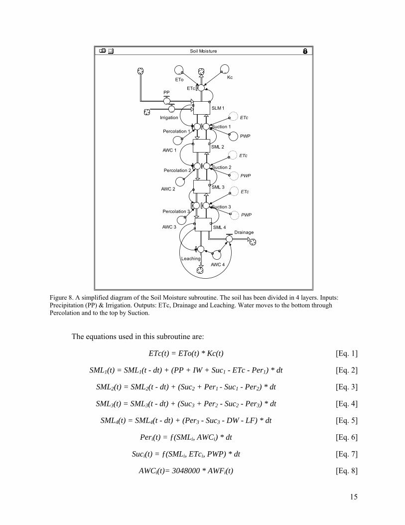
Mg (Total) % 0.34 0.30 0.24 0.28 0.23 0.23 0.19 0.22 Na (Total) ppm 6,510 3,868 4,903 4,298 5,968 3,741 4,653 4,385 Zn (Total) ppm 32 29 26 25 45 41 37 38 Mn (Total) ppm 58 68 65 75 42 47 47 64 Fe (Total) ppm 480 197 274 195 138 103 136 113 Cu (Total) ppm 13.5 13.3 11.6 12.0 13.7 13.0 15.5 13.1 Mo ppm 1.0 1.2 0.9 1.0 0.5 0.5 0.4 0.4 Se (Total) ppm 0.06 0.12 0.06 <0.05 <0.05 <0.05 <0.05 <0.05 As (Total) ppm 0.18 0.13 0.28 0.22 0.11 0.08 0.18 0.15 2. Formulation of a simple model to predict Bermuda grass growth and quality as a function of water use, N fertility and soil salinity The parameters values obtained from the pot trial were used to formulate a dynamic simulation model in Stella ®. The model was validated with data from the field by comparing model predictions to observed data. These model and data comparisons are reported elsewhere (Alonso et al., In review). A simplified version of the Stella® model was formulated in MS Excel for easy use by farmers growing forages in saline soils and others interested in using forages to manage saline water supplies. The model The model integrates the different components in 5 subroutines: Soil moisture; soil salinity; soil trace minerals (B, Mo and Se); plant yield and quality; and grazing. Simplified diagrams and brief descriptions of the subroutines indicating flows and stocks are shown below. Soil moisture In Soil Moisture (Figure 8) the soil has been divided in 4 layers 30cm deep each. There are two inflows, Irrigation (IW) and Precipitation (PP), and three outflows, ETc, Drainage and Leaching. ETc depends on ETo and Kc, and was directly measured at the experimental site by a surface renewal station (CR1000) in the growing season 2007-2008. ETo values integrate air temperature, day length and wind speed measurements, and are download online from the CIMIS station at Stratford. Kc values vary along the growing season and were estimated using ETo and ETc values in a software developed for this purpose at UC Davis (Snyder 2008).

15

Kc~

AWC 1

ETo

~

AWC 2

AWC 3

ETc

ETc

ETc

PWP

PWP

PWP

AWC 4

SLM 1

SML 2

SML 3

SML 4

Percolation 1

Percolation 2

Percolation 3

Leaching

Drainage

ETcPP

~

Irrigation

~

Suction 1

Suction 2

Suction 3

Soil Moisture

Figure 8. A simplified diagram of the Soil Moisture subroutine. The soil has been divided in 4 layers. Inputs: Precipitation (PP) & Irrigation. Outputs: ETc, Drainage and Leaching. Water moves to the bottom through Percolation and to the top by Suction. The equations used in this subroutine are:

ETc(t) = ETo(t) * Kc(t) [Eq. 1]

SML1(t) = SML1(t - dt) + (PP + IW + Suc1 - ETc - Per1) * dt [Eq. 2]

SML2(t) = SML2(t - dt) + (Suc2 + Per1 - Suc1 - Per2) * dt [Eq. 3]

SML3(t) = SML3(t - dt) + (Suc3 + Per2 - Suc2 - Per3) * dt [Eq. 4]

SML4(t) = SML4(t - dt) + (Per3 - Suc3 - DW - LF) * dt [Eq. 5]

Peri(t) = ƒ(SMLi, AWCi) * dt [Eq. 6]

Suci(t) = ƒ(SMLi, ETci, PWP) * dt [Eq. 7]

AWCi(t)= 3048000 * AWFi(t) [Eq. 8]

16

Where: (t) = Time t ETc = Crop evapotranspiration (L/ha*d) ETo = Potential evapotranspiration (L/ha*d) Kc = Crop coefficient SMLi = Soil moisture layer I (L/ha) PP = Precipitation (L/ha*d) IW = Irrigation water (L/ha*d) Suci = Suction to upper soil layer i (L/ha*d) Peri = Percolation from upper soil layer i (L/ha*d) DW = Drainage water (L/ha*d) LF = Leaching fraction (L/ha*d) AWCi = Available water capacity soil layer i (L/ha) PWP = Permanent wilting point (L/ha) AWFi = Available water fraction soil layer i (L) INIT = Initial values at t=0 And: AWF1 = 0.12 AWF2 = 0.08 AWF3 = 0.08 AWF4 = 0.06 INIT SML1 = 365760/3 INIT SML2 = 243840/2 INIT SML3 = 243840/2 INIT SML4 = 182880/2 PWP = 30480 Drainage and Leaching are functions of the water inputs through Precipitation and Irrigation, and the available water capacity of the soil (Σ AWCi). Soil salinity Salts flow through the soil profile dissolved in water. In the Soil Salinity subroutine (Figure 9) ECe values are transformed to total dissolved solids (TDS). TDS in the Soil (TDS Soil) depend on the balance of TDS in the irrigation water (TDS iw), drainage water (TDS drainage), leaching fraction (TDS leaching) and plant uptake (TDS plant uptake). TDS in the irrigation water are estimated through the volume of irrigation and its electrical conductivity (ECiw). TDS move through the soil profile due forces of evapotranspiration and percolation.

17

IW TDS

F maxETc

TDS SL 1

TDS SL 2

TDS SL 3

TDS SL 4

TDS Per 1

TDS Per 2

TDS Per 3

TDS LF

TDS DW

TDS Plant Uptake

TDS IW

Irrigation ~

TDS Suc 1

TDS Suc 2

TDS Suc 3

Soil Salinity

Figure 9. A simplified diagram of the Soil Salinity subroutine. The soil has been divided in 4 layers. The equations used in this subroutine are: TDS_SL1(t) = TDS_SL1(t - dt) + (TDS_IW + TDS_Suc1 – TDS_Per1 – TDS_PU) * dt [Eq. 9] TDS_SL2(t) = TDS_SL2(t - dt) + (TDS_Per1 + TDS_Suc2 – TDS_Per2 – TDS_Suc1)* dt [Eq. 10] TDS_SL3(t) = TDS_SL3(t - dt) + (TDS_Per2 + TDS_Suc3 – TDS_Per3 – TDS_Suc2)* dt [Eq. 11] TDS_SL4(t) = TDS_SL4(t - dt) + (TDS_Per3 – TDS_Suc3 – TDS_DW – TDS_LF) * dt [Eq. 12]

TDS_IW(t) = ƒ(IW, IWTDS) * dt [Eq. 13]

TDS_Peri(t) = ƒ(TDS_SLi, Peri) * dt [Eq. 14]

TDS_Suci(t) = ƒ(TDS_SLi+1, Suci) * dt [Eq. 15]

18

TDS_PU(t) = ƒ(ETc, Fmax) * dt [Eq. 16]

Where: (t) = Time t TDS_IW(t) = Total dissolved solids in the irrigation water (gr) IW(t) = Irrigation water (L) IWTDS(t) = Concentration of TDS in the irrigation water (gr/L) TDS_SLi(t) = TDS in the soil layer i (gr) TDS_Peri(t) = TDS in percolation water from the soil layer i TDS_Suci(t) = TDS in suction water from the soil layer i TDS_PU(t) = TDS in plant uptake (gr) TDS_DW(t) = TDS in drainage water (gr) TDS_LF(t) = TDS in leaching fraction (gr) Fmax(t) = Maximum plant uptake rate of TDS (mg/L*d) And:

INIT TDS_SL1 = 10304*SML1 TDS_IW = 740*ECiw, IF ECiw<5 dS/m INIT TDS_SL2 = 15180*SML2 TDS_IW = 840*ECiw, IF ECiw = 5-10 dS/m INIT TDS_SL3 = 19780*SML3 TDS_IW = 920*ECiw, IF ECiw>10 dS/m INIT TDS_SL4 = 20700*SML4 Fmax = 29.6 mg/L*d

Soil trace minerals The flow and accumulation of boron, selenium and molybdenum in the soil and plant tissues are described in the subroutine Soil Trace Minerals (Figure 10). The concentration of minerals in the soil depend on the initial content plus the additions through irrigation water (volume of water added multiplied by the concentration of the mineral in the water) minus the losses through drainage, leaching and plant uptake.

Yield Yield Yield

Irrigation

~

Irrigation

~

Irrigation

~

Drainage DrainageDrainage

B Leaching

Se Soil Mo Soil

Se Leaching

Se Irrigation

Mo Leaching

Se Drainage

B Plant Tissues

IW Se

Se Plant TissuesMo Plant Tissues

Mo Irrigation Mo Drainage

Se Uptake

IW MoSe dw

B SoilB Irrigation B Drainage

IW B

B Uptake Mo Uptake

B dw Mo dw

Trace Minerals

Figure 10. A simplified flow diagram of the subroutine of Trace Minerals (B, Se & Mo) indicating inflows and outflows.

19

The equations used in this subroutine are:

B_Soil(t) = B_Soil(t - dt) + (B_IW - B_DW - B_LF - B_PU) * dt [Eq. 17]

Se_Soil(t) = Se_Soil(t - dt) + (Se_IW - Se_DW - Se_LF - Se_PU) * dt [Eq. 18]

Mo_Soil(t) = Mo_Soil(t - dt) + (Mo_IW - Mo_DW - Mo_LF - Mo_PU) * dt [Eq. 19]

B_IW(t) = ƒ(IW, IWB) * dt [Eq. 20]

Se_IW(t) = ƒ(IW, IWSe) * dt [Eq. 21]

Mo_IW(t) = ƒ(IW, IWMo) * dt [Eq. 22]

B_PU(t) = ƒ(Yield, B_PT) * dt [Eq. 23]

Se_PU(t) = ƒ(Yield, Se_PT) * dt [Eq. 24]

Mo_PU(t) = ƒ(Yield, Mo_PT) * dt [Eq. 25] Where: B_Soil(t) =Boron in the soil (gr) B_IW(t) = Boron in irrigation water (gr) B_DW(t) =Boron in drainage water (gr) B_LF(t) = Boron in leaching fraction (gr) B_PU(t) = Plant uptake of boron (gr) B_PT(t) = Boron in plant tissues (ppm) IWB(t) = Concentration of boron in irrigation water (ppm) Se_Soil(t) = Selenium in the soil (gr) Se_IW(t) = Selenium in irrigation water (gr) Se_DW(t) = Selenium in drainage water (gr) Se_LF(t) = Selenium in leaching fraction (gr) Se_PU(t) = Plant uptake of selenium (gr) Se_PT(t) = Selenium in plant tissues (ppm) IWSe(t) = Concentration of selenium in irrigation water (ppm) Mo_Soil(t) = Molybdenum in the soil (gr) Mo_IW(t) = Molybdenum in irrigation water (gr) Mo_DW(t) = Molybdenum in drainage water (gr) Mo_LF(t) = Molybdenum in leaching fraction (gr) Mo_PU(t) = Plant uptake of molybdenum (gr) Mo_PT(t) = Molybdenum in plant tissues (ppm) IWMo(t) = Concentration of molybdenum in irrigation water (ppm) And: INIT B_Soil = 17.9*460955 INIT Se_Soil = 0.0125*460955 INIT Mo_Soil = 0.8351*460955

20

Plant yield and quality In the subroutine Plant Yield and Quality (Figure 11), crop yield is function of crop growth. Harvest is the fraction of total yield that is used. In a grazing system, Harvest depends on the grazing efficiency (H) of the pasture. Grazing efficiencies can range from 40% in a continuous grazing system to 80% in a rotational system.

Yield

Growth

r

Leaves Stems

N

~

LSR

Harvest

~

H

ECe Soil

Plant Yield and Quality

Figure 11. A simplified flow diagram of the subroutine Plant Yield and Quality indicating inflows and outflows.

Yield(t) = Yield(t - dt) + (Growth - Harvest) * dt [Eq. 26] Where: Yield(t) = Total yield (kg/ha) Growth(t) = Plant growth (kg/ha*d) Harvest(t) = Fraction of the total yield harvested (kg/ha) Growth is described by a logistic curve where the intrinsic growth rate (r) is affected by the level of nitrogen (N) and soil Salinity (ECe Soil). Response functions were obtained from the pot trial and tested against field data. Figure 12 shows the average growth rate of Bermuda grass under different levels of nitrogen fertilization.

Average Growth Rate at the Pot Trial

0.0

0.2

0.4

0.6

0.8

1.0

1.2

1.4

1.6

140 180 220 260 300 340

DOY

g/d

AVG-N0

AVG-N1

AVG-N2

Poly. (AVG-N2)

Poly. (AVG-N1)

Poly. (AVG-N0)

Figure 12. Average growth rate of Bermuda grass at the pot trial under different nitrogen levels based on pooled samples from 2007 and 2008. N0: 0 kg N ha-1; N1: 300 kg N ha-1; N2: 600 kg N ha-1; DOY: Day of the year.

21

Growth(t) = ƒ(r) * dt [Eq. 26]

r(t) = ƒ(N, ECe_Soil) * dt [Eq. 27]

Harvest(t) = Yield(t) * H(t) [Eq. 28]

LSR(t) = ƒ(N) * dt [Eq. 29]

Where: r(t) = Intrinsic growth rate (kg/ha*d) N(t) = Nitrogen added in the water or as fertilizer (kg/ha) ECe_Soil(t) = Soil salinity (dS/m) H(t) = Harvest efficiency (%) LSR(t) = Leaf-stem ratio And:

LSR(t) = -4E-05 * t2 + 0.0272 * t – 2.4212 IF N = 0 LSR(t) = 0.0001 * t2 – 0.0411 * t + 5.6414 IF N > 0 r(t)¥ = -0.0039 * t2 + 0.817 * t + 3.4132 IF N = 0 r(t)¥= -0.0046 * t2 + 1.1487 * t – 1.4509 IF N >300 kg/ha & soil ECe > 7dS/m r(t)¥ =-0.0052 * t2 + 1.3987 * t – 3.8312 IF N >300 kg/ha & soil ECe < 7dS/m

(t)¥ = Days after seeding

Finally, in the subroutine Grazing (Figure 13) the model estimates the optimum stocking rate (SR) for the pasture given the forage yield and the average daily weight gain (ADG). It also predicts the maximum average daily weight gain per animal unit given the forage yield and the stocking rate. Grazing

ADG

H

~

Km

Kwg

CC

MEm

MEwg

Weight

ADG

Yield

CC

ME TOT Pasture

STOCKING RATE

REMm HERD

MEm

ME DISPwg

Max ADG in PASTURE

KwgWeight

Weight

MEm

MEwgRME TOT

RDM TOT

CC

Cumulative Intake

Daily Itake

RDM TOT

Yield

STOCKING RATE

STOCKING RATE

Grazing

Figure 13. Subroutine Grazing.

22

In this subroutine the requirements of dry matter and metabolic energy for maintenance

and weight gain of grazing animals are matched with the forage dry matter and energy supply on a daily basis, identifying the dates where the animals require supplementation at any given stocking rate. The principal equations are:

RME_TOT(t) = MEm(t) + MEwg(t) [Eq. 30]

MEm(t) = (5.67 + 0.061 * Weight(t)) / Km(t) [Eq. 31]

MEwg(t) = ((ADG * (6.28+0.0188 * Weight)) / (1-0.3 * ADG)) / Kwg(t) [Eq. 32]

RDM_TOT(t) = RME_TOT(t) / CC(t) [Eq. 33]

Weight(t) = Weight(t - dt) + ADG * dt [Eq. 34]

STOCKING_RATE(t) = (Yield(t) * H(t)) / Cumulative_Intake(t) [Eq. 35]

REMm_HERD(t) = MEm(t) * STOCKING_RATE(t) * 1.05 [Eq. 36]

ME_DISPwg(t) = ME_TOT_Pasture(t) - REMm_HERD(t) [Eq. 37] Max ADG in PASTURE (t) = ((ME_DISPwg(t) * Kwg(t)) / (6.28 + 0.0188 *

Weight(t) + 0.3 * ME_DISPwg(t) * Kwg(t)) / STOCKING_RATE(t)

[Eq. 38]

Where: RME_TOT(t) = Total requirement of metabolic energy (Mj) MEm(t) = Requirement of metabolic energy for maintenance (Mj) MEwg(t) = Requirement of metabolic energy for weight gain (Mj) Weight(t) = Live weight (kg) Km(t) = Maintenance efficiency (%) Kwg(t) = Weight gain efficiency (%) RDM_TOT(t) = Total requirement of dry matter (kg) ADG(t) = Average daily gain of weight (kg/d) CC(t) = Caloric concentration of the pasture (Mj) STOCKING_RATE(t) = Stocking Rate (AU/ha) Cumulative_Intake(t) = Intake of an AU(kg) REMm_HERD(t) = Herd requirement of metabolic energy for maintenance (Mj) ME_DISPwg(t) = Metabolic energy available for weight gain (Mj) ME_TOT_Pasture(t) = Total metabolic energy of the pasture (Mj) Max ADG in PASTURE (t) = Max possible ADG per AU in the pasture (kg/d) And: Km(t) = 0.55 + 0.016 * CC Kwg(t) = 0.0435 * CC

23

Model validation and testing Forage yield and quality The model performance was tested using data collected at the research site in 2001 and 2003. Field data and the corresponding predictions by the model were paired and analyzed. Predictions of crop yield under different soil salinity levels match field data. Table 6 shows the standing biomass pre-grazing at WLF in 2001. Figure 14 shows the fit between the observed and predicted yield values for that year.

Table 6. Field values of forage production at WLF Pre-Grazing (kg/ha)

Date Paddock 2 Paddock 3 Paddock 6 Paddock 7 June-01 2,062 3,125 1,734 1,774 July-01 6,654 6,669 5,190 5,567

August-01 4,630 7,800 8,047 6,956 September-01 5,480 5,345 10,266 7,095

October-01 5,855 5,214 9,584 6,906

Predicted vs Observed Yield (2001)

0

2000

4000

6000

8000

10000

12000

12

1

13

3

14

5

15

7

16

9

18

1

19

3

20

5

21

7

22

9

24

1

25

3

26

5

27

7

28

9

30

1

DOY

kg D

M/h

a

OBS Paddock 2

OBS Paddock 3

OBS Paddock 6

OBS Paddock 7

Pedicted N450

Figure 14: Observed and predicted Bermuda grass yields in 2001.

The fit between model predictions and observed values of forage quality is reasonable good also. Figures 15-18 show the model fit for ADF, NDF, crude protein, ash, B, Se and Mo. 95% confidence intervals for the mean of field data samples on each parameter were built and model predictions were tested against them. Figures shown correspond to the year with higher number of observations.

24

Predicted vs Observed ADF 2003

26

27

28

29

30

31

32

33

34

50 100 150 200 250 300 350

DOY

%

Predicted Mean

Observed Mean

Predicted vs Observed NDF 2003

50

55

60

65

70

75

0 50 100 150 200 250 300 350

DOY

%

Predicted Mean

Observed Mean

Figure 15. Model fit for ADF and NDF values in Bermuda grass.

Predicted vs Observed Crude Protein 2003

6

7

8

9

10

11

0 50 100 150 200 250 300 350

DOY

%

Predicted Mean

Observed Mean

Predicted vs Observed Ash 2003

8.0

8.5

9.0

9.5

10.0

10.5

11.0

11.5

50 100 150 200 250 300 350

DOY

%

Predicted Mean

Observed Mean

Figure 16. Model fit for crude protein and ash values in Bermuda grass.

Predicted vs Observed Boron 2003

140

160

180

200

220

240

260

280

0 50 100 150 200 250 300 350

DOY

pp

m Predicted Mean

Observed Mean

Predicted vs Observed Selenium 2001

40

50

60

70

80

90

100

110

0 50 100 150 200 250 300 350

DOY

pp

b Predicted Mean

Observed Mean

Figure 17. Model fit for crude boron and selenium values in Bermuda grass.

Predicted vs Observed Molybdenum 2003

0.0

0.2

0.4

0.6

0.8

1.0

1.2

0 50 100 150 200 250 300 350

DOY

pp

m Predicted Mean

Observed Mean

Figure 18. Model fit for molybdenum values in Bermuda grass.

25

Beef cattle production Table 7 shows the average daily gain (ADG) of weight of beef cattle grazing at the experimental site during 2001 and 2003.

Table 7. Average daily gain (ADG) of weigh of steers grazing at WLF during the growing seasons 2001 and 2003

Year Gazing Period Treatment Steers

Stocking Rate ADG SD

Days # Heads/ha kg/ha*d kg/ha*d 2001 143 Control 8 Low 0.56 0.09

143 Treatment 18 Low 0.46 0.23 2003 150 Control 10 Low 0.55 0.15

150 Treatment 30 Low 0.72 0.12

There is a good fit between the observed and predicted values of ADG. Figure 19 shows the daily gain predicted for the field conditions in 2001. Predicted values are within the rage of those observed at the field site at WLF.

Predicted ADG 2001

0.42

0.44

0.46

0.48

0.5

0.52

0.54

0.56

0.58

1

18

35

52

69

86

10

3

12

0

13

7

15

4

17

1

18

8

20

5

22

2

23

9

25

6

27

3

29

0

30

7

32

4

34

1

35

8

DOY

AD

G (

kg/d

)

Figure 19. Predicted maximum daily gain (ADG) for steers grazing Bermudagrass at WLF in 2001. Final Discussion Results of the model indicate the feasibility of growing Bermudagrass on the saline soils of the western San Joaquin Valley of California when irrigated with drainage water. Although leaf/stem ratio was not influenced by soil salinity, the effect of salinity and nitrogen levels greatly affected the total biomass produced. The model also shows the feasibility of grazing Bermudagrass with average daily gains of 0.7 kg ha*d-1 at low stocking rates or at least maintenance at higher stocking rates. Using crop–specific and site-specific (i.e. soil and irrigation) parameters’ values the model could be used to predict yield and quality for different pastures and crops cultivated under saline condition on the western San Joaquin Valley and elsewhere.

26

OTHER OUTPUTS OF THE PROJECT Recent Presentations Kaffka, S. and Alonso, M. 2008. Linking drainage water management in the Western San Joaquin Valley to bio-energy production. California Energy Commission’s Sustainability Working Group. December 5, Sacramento, California. Alonso, M., Kaffka, S. and Corwin, D. 2008. Bermuda Grass as an Alternative for Retired Farmland in the Western San Joaquin Valley of California. Farming with Grass Conference. October 20-22, Oklahoma City, Oklahoma. Alonso, M. and Kaffka, S. 2007. Modeling Bermuda Grass Yield and Quality in the Western San Joaquin Valley of California. American Society of Agronomy, Crop Science Society of America and Soil Science Society of America International Annual Meetings. November 4-8, New Orleans, Louisiana. Kaffka, S., Oster, J., Corwin, D., and Maas, J. 2007. Saline Drainage Water and its Effects on Forges and Livestock. American Society of Agronomy, Crop Science Society of America and Soil Science Society of America International Annual Meetings. November 4-8, New Orleans, Louisiana. Publications Alonso, M. F. and S. R. Kaffka. Bermuda grass (Cynodon dactylon (L.) Pers.) yield and quality under different levels of salinity, nitrogen and trace elements: A greenhouse experiment. (In review). Alonso, M. F. and S. R. Kaffka. Modeling Bermuda grass (Cynodon dactylon (L.) Pers.) production in the saline soils of the western San Joaquin Valley of California. (In review). Corwin, D.L., S. M. Lesch, J. D. Oster, and S. R. Kaffka. 2008. Short-term sustainability of drainage water reuse: Spatio-temporal impact on soil chemical properties. Journal of Environmental Quality 37, S8-S24. Kaffka, S. R., J. D. Oster and D. L. Corwin. 2004. Forage production and soil reclamation using saline drainage water. Pg 247-253 In: Proceedings, National Alfalfa Symposium, 13-15 December 2004, San Diego, California. UC Cooperative Extension, University of California, Davis.

Acknowledgements

The authors acknowledge the California Department of Water Resources for funding part of the field work, the sample analyses and the modeling effort and the University of California Salinity Drainage Program for funding the pot trial as well as field site preparation. The authors thank Ceil Howe III and Westlake Farms for the use of their land, and their efforts to provide and manage livestock and drainage waters to the site.

27

APPENDIX

28

ForageS

Simulation Model for

Forage Production in Saline Environments

Operation Guide

Version 1.1

for XLS

Maximo F. Alonso & Stephen R. Kaffka

University of California, Davis

July 2009

29

Table of Contents INTRODUCTION …………………………………………………………………. 3 INITIAL PARAMETER VALUES ………………………………………………... 3 INITIAL Soil Values …………………………………………………………. 3 INITIAL Crop values ………………………………………………………… 4 INITIAL Moisture values ……………………………………………………. 5 INITIAL Cattle values ……………………………………………………….. 6 INITIAL Trace minerals values ……………………………………………… 6 MODEL RESULTS ………………………………………………………………... 6 REFERENCES ……………………………………………………………………... 10 Appendix. Abbreviations .………………………...……………………………... 11

30

INTRODUCTION ForageS version 1.1 for XLS is a dynamic simulation model that runs in Excel™. The original version was developed in Stella™. The model has been formulated to predict forage production and beef cattle performance on saline environments. The present version has been validated for Bermuda grass (Cynodon dactylon (L.) Pers.) growing on the western San Joaquin Valley of California, and the examples used in this Operation Guide refer to it. For its operation the model requires the input of crop-specific and site-specific parameter values. This guide describes how to parameterize and operate the model. For more references see Alonso et al., (In review), Alonso and Kaffka, (In review) and Alonso and Kaffka, (2009).

The model uses daily Kc values to estimate ETc based on daily ETo values. Soil moisture, salinity and trace minerals are modeled as a mass balance among the different components of the system (soil, plant and atmosphere). The soil has been divided in four layers 0.3 m deep each, for a total depth of 1.2 m. Inputs to the system occur through precipitation, irrigation and fertilization. Outputs occur through harvest (plant uptake), drainage (including runoff), and leaching.

Crop response functions (Alonso and Kaffka, 2009) for forage yield and quality under different N and salinity levels obtained from greenhouse trails (Alonso and Kaffka, In review) are used to predict crop yield and quality on field conditions. Beef cattle stocking rates and average daily weight gains are estimated based on dry matter (DM) and energy balance between animal requirements and pasture yield.

Model predictions were tested against field data measurements (Alonso et al., In review). For this purpose, 95% confidence intervals for the mean of field data samples on each parameter were built and model predictions were tested against them. Model predictions fitted field data measurements.

Using crop and site specific parameters’ values the model can be used to simulate different scenarios and predict yield and quality of pastures on saline environments elsewhere.

INITIAL PARAMETER VALUES INITIAL Soil Values The soil has been divided in 4 layers. The model requires to define the depth (in) and the water capacity fraction (WCF; in/in) of each soil layer. This information is site-specific and can be obtained at http://soildatamart.nrcs.usda.gov/Default.aspx. Initial values are:

Value Unit Depth Soil Layer 1 12 in Depth Soil Layer 2 12 in Depth Soil Layer 3 12 in Depth Soil Layer 4 12 in

31

Value Unit Available Water Fraction SL1 0.12 in/in Available Water Fraction SL2 0.08 in/in Available Water Fraction SL3 0.08 in/in Available Water Fraction SL4 0.06 in/in * SL = Soil Layer

The model also requires specifying the permanent wilting point (%), ECe (dS/m), and the initial concentration of B (mg/L), Se (µg/L) and Mo (µg/L) in the soil. Initial values at the experimental site in the Western San Joaquin Valley (WSJV) are:

Value Unit Permanent Wilting Point SL1 1 % Permanent Wilting Point SL2 1 % Permanent Wilting Point SL3 1 % Permanent Wilting Point SL4 1 % Permanent Wilting Point Soil 1 % * SL = Soil Layer

Value Unit INIT ECe Soil Layer 1 11.2 dS/m INIT ECe Soil Layer 2 16.5 dS/m INIT ECe Soil Layer 3 21.5 dS/m INIT ECe Soil Layer 4 22.5 dS/m INIT ECe Soil AVG 17.9 dS/m

Value Unit INIT Soil Boron (B) 17.9 mg/L INIT Soil Selenium (Se) 12.5 μg/L INIT Soil Molybdenum (Mo) 835.1 μg/L

INITIAL Crop values The model uses crop-specific Kc values and daily ETo data to estimate daily ETc for the pasture. Kc values for Bermuda grass are shown below. ETo data from the closest CIMIS station can be acquired at http://wwwcimis.water.ca.gov/cimis/data.jsp.

Bermuda grass Kc values in WSJV Month Kc Month Kc

Jan - Jul 1.06 Feb - Aug 0.96 Mar 0.67 Sep 0.78 Apr 0.84 Oct 0.64 May 0.97 Nov 0.54 Jun 1.06 Dec -

Initial yield (lb DM/ac), N fertilization (lb N/ac) and maximum plant salt uptake rate (dS/m*d) values at the experimental site are:

32

Value Unit

INIT Yield 450 lb DM/ac

Nitrogen Fertilization (N) 360 lb N/ac

Maximum Salt Uptake Rate 0.2 dS/m*day INITIAL Moisture values The model requires the input of precipitation (in), and irrigation volume (acre-foot) and quality (dS/m). Precipitation data from the closest CIMIS station can be acquired at http://wwwcimis.water.ca.gov/cimis/data.jsp. Precipitation values at WSJV in 2001 used to validate the model are:

DOY * Date Precipitation

(in) DOY Date Precipitation

(in) 8 8-Jan 0.14 96 6-Apr 0.17

10 10-Jan 0.79 97 7-Apr 0.27 11 11-Jan 0.09 98 8-Apr 0.02 12 12-Jan 0.01 99 9-Apr 0.20 23 23-Jan 0.04 108 18-Apr 0.05 24 24-Jan 0.35 187 6-Jul 0.02 25 25-Jan 0.24 188 7-Jul 0.25 32 1-Feb 0.01 303 30-Oct 0.18 40 9-Feb 0.01 314 10-Nov 0.19 42 11-Feb 0.22 315 11-Nov 0.07 43 12-Feb 0.09 316 12-Nov 0.21 44 13-Feb 0.25 330 26-Nov 0.07 49 18-Feb 0.02 333 29-Nov 0.05 50 19-Feb 0.12 335 1-Dec 0.11 51 20-Feb 0.03 341 7-Dec 0.02 52 21-Feb 0.01 343 9-Dec 0.04 54 23-Feb 0.09 348 14-Dec 0.07 55 24-Feb 0.30 354 20-Dec 0.05 56 25-Feb 0.06 358 24-Dec 0.01 57 26-Feb 0.24 359 25-Dec 0.01 59 28-Feb 0.02 360 26-Dec 0.01 62 3-Mar 0.10 362 28-Dec 0.07 63 4-Mar 0.65 363 29-Dec 0.25 64 5-Mar 0.54 364 30-Dec 0.15 68 9-Mar 0.08 365 31-Dec 0.01

* DOY: Day of the year Irrigation data at WSJV in 2001 used to validate the model is shown below:

DOY

Date Irrigation

(acre-foot) ECiw

(dS/m) 156 5-Jun 0.481 8.7199 18-Jul 0.356 14.4214 2-Aug 0.252 11.5

33

234 22-Aug 0.358 16.2257 14-Sep 0.28 12.7271 28-Sep 0.191 12.7

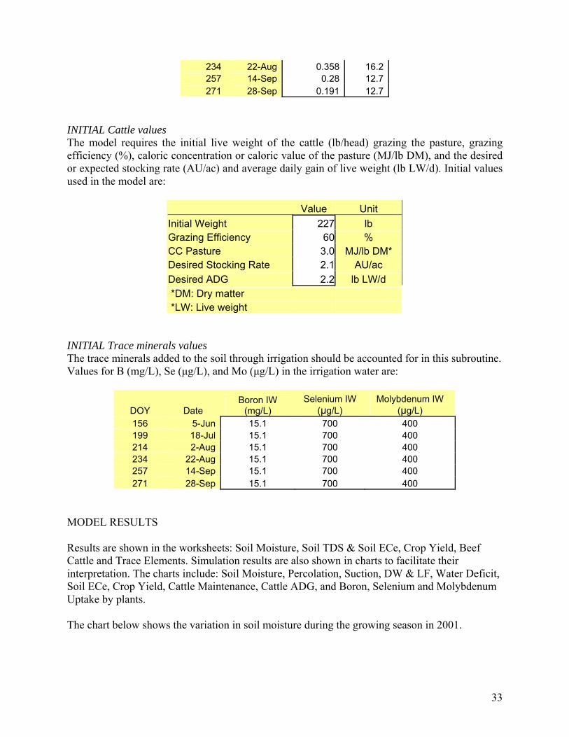
INITIAL Cattle values The model requires the initial live weight of the cattle (lb/head) grazing the pasture, grazing efficiency (%), caloric concentration or caloric value of the pasture (MJ/lb DM), and the desired or expected stocking rate (AU/ac) and average daily gain of live weight (lb LW/d). Initial values used in the model are:

Value Unit

Initial Weight 227 lb Grazing Efficiency 60 % CC Pasture 3.0 MJ/lb DM* Desired Stocking Rate 2.1 AU/ac

Desired ADG 2.2 lb LW/d *DM: Dry matter *LW: Live weight

INITIAL Trace minerals values The trace minerals added to the soil through irrigation should be accounted for in this subroutine. Values for B (mg/L), Se (μg/L), and Mo (μg/L) in the irrigation water are:

DOY Date Boron IW

(mg/L) Selenium IW

(µg/L) Molybdenum IW

(μg/L) 156 5-Jun 15.1 700 400 199 18-Jul 15.1 700 400 214 2-Aug 15.1 700 400 234 22-Aug 15.1 700 400 257 14-Sep 15.1 700 400 271 28-Sep 15.1 700 400

MODEL RESULTS Results are shown in the worksheets: Soil Moisture, Soil TDS & Soil ECe, Crop Yield, Beef Cattle and Trace Elements. Simulation results are also shown in charts to facilitate their interpretation. The charts include: Soil Moisture, Percolation, Suction, DW & LF, Water Deficit, Soil ECe, Crop Yield, Cattle Maintenance, Cattle ADG, and Boron, Selenium and Molybdenum Uptake by plants. The chart below shows the variation in soil moisture during the growing season in 2001.

34

SOIL MOISTURE

0.00

1.00

2.00

3.00

4.00

5.00

6.00

7.00

1 15 29 43 57 71 85 99 113 127 141 155 169 183 197 211 225 239 253 267 281 295 309 323 337 351 365

DOY

acre

-in

chMoisture Soil Layer 1(acre-inch)

Moisture Soil Layer 2(acre-inch)

Moisture Soil Layer 3(acre-inch)

Moisture Soil Layer 4(acre-inch)

SoilMoisture(acre-inch)

The chart below shows the variation in soil ECe during the growing season in 2001.

Soil ECe

0.0

5.0

10.0

15.0

20.0

25.0

30.0

35.0

40.0

45.0

50.0

1 15 29 43 57 71 85 99 113 127 141 155 169 183 197 211 225 239 253 267 281 295 309 323 337 351 365

DOY

dS

/m

ECe SL1(dS/m)

ECe SL2(dS/m)

ECe SL3(dS/m)

ECe SL4(dS/m)

ECe Soil(dS/m)

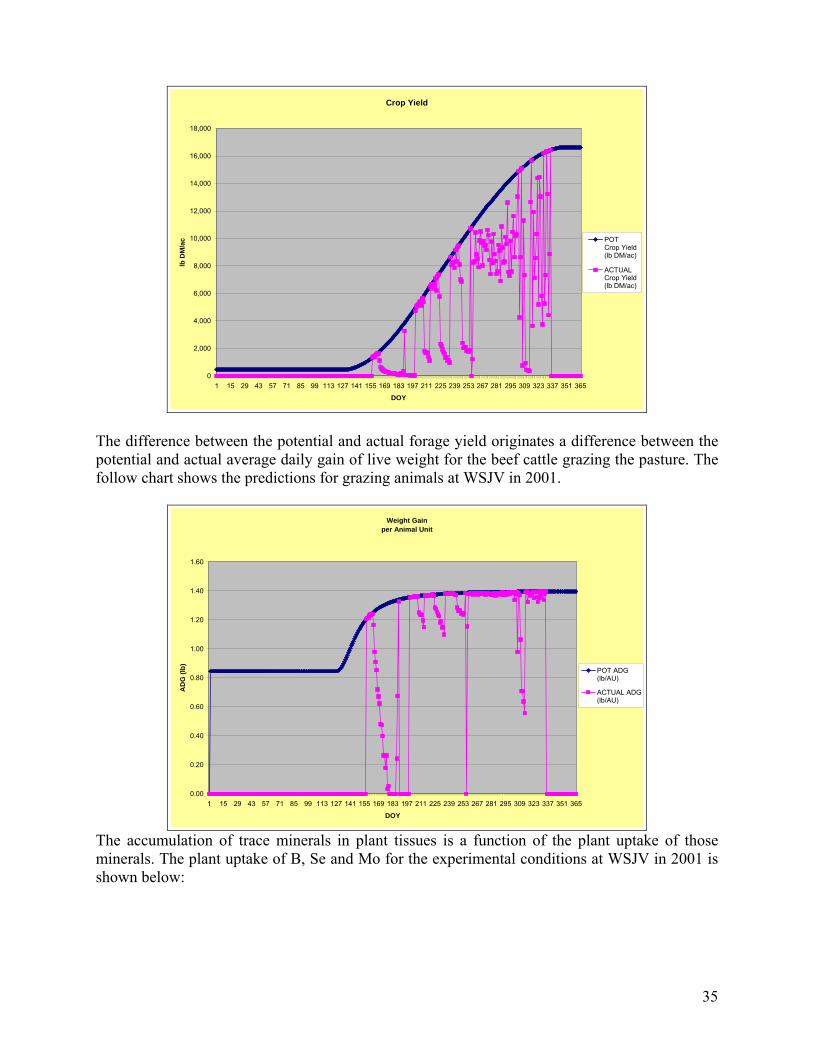
The potential yield is function of the soil and irrigation water salinity, and nitrogen fertilization level. When under-irrigation does not allow the crop to express its potential, the actual yield is lower than the potential yield. The chart below shows the difference between the actual and the potential yield at WSJV in 2001.

35

Crop Yield

0

2,000

4,000

6,000

8,000

10,000

12,000

14,000

16,000

18,000

1 15 29 43 57 71 85 99 113 127 141 155 169 183 197 211 225 239 253 267 281 295 309 323 337 351 365

DOY

lb D

M/a

c POTCrop Yield(lb DM/ac)

ACTUALCrop Yield(lb DM/ac)

The difference between the potential and actual forage yield originates a difference between the potential and actual average daily gain of live weight for the beef cattle grazing the pasture. The follow chart shows the predictions for grazing animals at WSJV in 2001.

Weight Gain

per Animal Unit

0.00

0.20

0.40

0.60

0.80

1.00

1.20

1.40

1.60

1 15 29 43 57 71 85 99 113 127 141 155 169 183 197 211 225 239 253 267 281 295 309 323 337 351 365

DOY

AD

G (

lb)

POT ADG(lb/AU)

ACTUAL ADG(lb/AU)

The accumulation of trace minerals in plant tissues is a function of the plant uptake of those minerals. The plant uptake of B, Se and Mo for the experimental conditions at WSJV in 2001 is shown below:

36

Plant Uptakeof Boron

0.00

20.00

40.00

60.00

80.00

100.00

120.00

140.00

160.00

180.00

1 15 29 43 57 71 85 99 113 127 141 155 169 183 197 211 225 239 253 267 281 295 309 323 337 351 365

DOY

pp

m Plant UptakeBoron(ppm)

Plant Uptake ofSelenium

0.00

0.20

0.40

0.60

0.80

1.00

1.20

1.40

1.60

1.80

1 15 29 43 57 71 85 99 113 127 141 155 169 183 197 211 225 239 253 267 281 295 309 323 337 351 365

DOY

pp

m Plant UptakeSelenium(ppm)

Plant Uptake ofMolybdenum

0.00

0.20

0.40

0.60

0.80

1.00

1.20

1.40

1.60

1.80

1 15 29 43 57 71 85 99 113 127 141 155 169 183 197 211 225 239 253 267 281 295 309 323 337 351 365

DOY

pp

m Plant UptakeMolybdenum(ppm)

37

REFERENCES Alonso, M. F., Corwin, D., Oster, J., Maas, J. and Kaffka, S.R. Modeling Bermuda grass (Cynodon dactylon (L.) Pers.) production in the saline soils of the western San Joaquin Valley of California. (In review). Alonso, M. F. and S.R. Kaffka. (In review). Bermuda grass (Cynodon dactylon (L.) Pers.) yield

and quality under different levels of salinity, nitrogen and trace elements: A greenhouse evaluation

Alonso, M. F. and S.R. Kaffka. 2009. Predicting water use, crop growth and quality of Bermuda

grass under saline irrigation. Final Report for the California Department of Water Resources. Contract

38

Appendix A: Abbreviations

ADG Average daily gain (lb) AU Animal unit AWC Available water capacity (in/in) B Boron (mg) CIMIS California Irrigation Management Information System DM Dry matter (lb) DOY Day of the year ECdw Electrical conductivity drainage water (dS/m) ECe Electrical conductivity paste extract (dS/m) ECiw Electrical conductivity irrigation water (dS/m) ETa Actual evapo-transpiration (in) ETc Crop evapo-transpiration (in) ETo Potential evapotranspiration (in) Kc Crop coefficient LW Live weight (lb) Mo Molybdenum (µg) N Nitrogen (lb) Se Selenium (µg) TDS Total dissolved solids (mg) WCF Water capacity fraction (in/in) WSJV Western San Joaquin Valley