predicting surface scatter using a linear systems
TRANSCRIPT

University of Central Florida University of Central Florida
STARS STARS
Electronic Theses and Dissertations, 2004-2019
2006
Predicting Surface Scatter Using A Linear Systems Formulation Of Predicting Surface Scatter Using A Linear Systems Formulation Of
Non-paraxial Scalar Diffraction Non-paraxial Scalar Diffraction
Andrey Krywonos University of Central Florida
Part of the Electromagnetics and Photonics Commons, and the Optics Commons
Find similar works at: https://stars.library.ucf.edu/etd
University of Central Florida Libraries http://library.ucf.edu
This Doctoral Dissertation (Open Access) is brought to you for free and open access by STARS. It has been accepted
for inclusion in Electronic Theses and Dissertations, 2004-2019 by an authorized administrator of STARS. For more
information, please contact [email protected].
STARS Citation STARS Citation Krywonos, Andrey, "Predicting Surface Scatter Using A Linear Systems Formulation Of Non-paraxial Scalar Diffraction" (2006). Electronic Theses and Dissertations, 2004-2019. 1086. https://stars.library.ucf.edu/etd/1086

PREDICTING SURFACE SCATTER USING A LINEAR SYSTEMS FORMULATION OF NON-PARAXIAL SCALAR DIFFRACTION
by
ANDREY KRYWONOS B.S. State University of New York Institute of Technology, 1995
M.S. University of Central Florida, 2000
A dissertation submitted in partial fulfillment of the requirements for the degree of Doctor of Philosophy in the College of Optics and Photonics
at the University of Central Florida Orlando, Florida
Fall Term 2006
Major Professor: James E. Harvey

ii
© 2006 Andrey Krywonos

iii
ABSTRACT
Scattering effects from rough surfaces are non-paraxial diffraction phenomena
resulting from random phase variations in the reflected wavefront. The ability to predict
these effects is important in a variety of applications including x-ray and EUV imaging,
the design of stray light rejection systems, and reflection modeling for rendering realistic
scenes and animations of physical objects in computer graphics.
Rayleigh-Rice (small perturbation method) and Beckmann-Kirchoff (Kirchhoff
approximation) theories are commonly used to predict surface scatter effects. In addition,
Harvey and Shack developed a linear systems formulation of surface scatter phenomena
in which the scattering behavior is characterized by a surface transfer function. This
treatment provided insight and understanding not readily gleaned from the two previous
theories, and has been incorporated into a variety of computer software packages (ASAP,
Zemax, Tracepro). However, smooth surface and paraxial approximations have severely
limited the range of applicability of each of the above theoretical treatments.
In this dissertation, a linear systems formulation of non-paraxial scalar diffraction
theory is first developed and then applied to sinusoidal phase gratings, resulting in
diffraction efficiency predictions far more accurate than those provided by classical
scalar theories. The application of the theory to these gratings was motivated by the fact
that rough surfaces are frequently modeled as a superposition of sinusoidal surfaces of
different amplitudes, periods, and orientations.
The application of the non-paraxial scalar diffraction theory to surface scatter
phenomena resulted first in a modified Beckmann-Kirchhoff surface scattering model,

iv
then a generalized Harvey-Shack theory, both of which produce accurate results for
rougher surfaces than the Rayleigh-Rice theory and for larger incident and scattering
angles than the classical Beckmann-Kirchhoff theory. These new developments enable
the analysis and simplify the understanding of wide-angle scattering behavior from rough
surfaces illuminated at large incident angles. In addition, they provide an improved
BRDF (Bidirectional Reflectance Distribution Function) model, particularly for the
smooth surface inverse scattering problem of determining surface power spectral density
(PSD) curves from BRDF measurements.

v
This work is dedicated to the memory of my brother
Volodimir Krywonos (1969-1985)
You left us far too soon, and I miss you.

vi
ACKNOWLEDGMENTS
There have been a number of people throughout my career as a graduate student
who have helped me, inspired me, and generally made it all worthwhile. To these people,
I give my heartfelt thanks.
First I thank my advisor, James Harvey, for the opportunity to work with you over
these many years on many interesting projects. It was truly an honor. Your insight,
enthusiasm, patience, and dedication to your students are but a few of your numerous
qualities. I have thoroughly enjoyed all of our discussions, both technical and not, and
am grateful that your door was always open. I could not have done this without you.
I would also like to offer thanks to each of the members of my committee, both
for agreeing to serve as members and because each of them has had an impact on me
during my time here:
• Glenn Boreman - without a doubt the best classroom teacher I have
ever had.
• Jannick Rolland - because the things you taught me I have used a
thousand times (maybe a million!)
• Richard Eastes - for the opportunity to work on an extremely
interesting project, and for all of your support.
I thank John Stover for generously providing some of the scattering
measurements used in this dissertation.

vii
I give enormous thanks to my parents, Very Rev. Mykola and Rita Krywonos,
who have always supported me whether they agreed with me or not. They have always
done their best to be the best parents they could be, and they have truly succeeded.
I thank the following people for their friendship and support:
• Dan Durfey - because if you hadn’t, I probably wouldn’t have either,
and because you’re the best friend a person could ever hope to have.
• Javier Gonzalez - for all of your advice, for your tennis lessons, and
for making it bearable when it didn’t seem bearable.
• Larry D. Davis, Jr. - for letting me beat you at racquetball, for Epic
Gatherings, and for being someone I can always count on.
• Gabriel Popescu - for road trips to Boston, for your movie making
skills, and for making things interesting.
• Ferenc Szipőcs - for Ali G, Monty P, and for lots of interesting
conversations.
• Cindi Vernold - for all of your help early on
Thanks to Caroline for your endless supply of smiles. You may have slowed me
down a little bit, but it was worth every minute.
Last, but most of all, I thank my wonderful wife Betsy for all of her love, support,
patience, and understanding. And for putting up with all of my illustrated explanations. I
don’t know how you do it, but you do it so well, and I’m eternally grateful.

viii
TABLE OF CONTENTS
LIST OF FIGURES ........................................................................................................... xi
LIST OF TABLES......................................................................................................... xviii
TABLE OF ACRONYMS/ABBREVIATIONS.............................................................. xix
CHAPTER 1: INTRODUCTION....................................................................................... 1
1.1 Surface Scatter Phenomena....................................................................................... 1
1.2 Motivation And Goals For This Research ................................................................ 5
1.3 Organization Of This Dissertation ............................................................................ 7
CHAPTER 2: HISTORICAL BACKGROUND ................................................................ 9
2.1 Scalar Diffraction Theory ......................................................................................... 9
2.1.1 Fresnel And Fraunhofer Diffraction ................................................................ 15
2.1.1.1 The Fresnel Approximation ...................................................................... 15
2.1.1.2 The Fraunhofer Approximation ................................................................ 16
2.1.2 Fourier Treatment Of Non-Paraxial Scalar Diffraction Theory ...................... 18
2.1.2.1 The Angular Spectrum Of Plane Waves................................................... 19
2.1.2.2 The Diffracted Wave Field As A Superposition Of Spherical Waves...... 23
2.1.2.3 Aberrations Of Diffracted Wave Fields.................................................... 26
2.2 Surface Scatter Theory............................................................................................ 28
2.2.1 The Bidirectional Reflectance Distribution Function (BRDF)........................ 31
2.2.2 Rayleigh-Rice (Small Perturbation) Surface Scatter Theory........................... 34
2.2.3 Beckmann-Kirchhoff Surface Scatter Theory ................................................. 38
2.2.4 Harvey-Shack Surface Scatter Theory............................................................. 49

ix
CHAPTER 3: A LINEAR SYSTEMS FORMULATION OF NON-PARAXIAL SCALAR DIFFRACTION THEORY............................................................................ 57
3.1 Radiometric Terminology....................................................................................... 61
3.2 Diffracted Radiance – A Fundamental Quantity .................................................... 63
3.3 Renormalization Conserves Energy In The Presence Of Evanescent Waves......... 66
3.4 Application To Sinusoidal Phase Gratings ............................................................. 72
3.4.1 Paraxial Model Of Sinusoidal Phase Gratings................................................. 73
3.4.2 Wide-Angle Behavior Of Sinusoidal Phase Gratings...................................... 78
3.4.3 Prediction Of Diffraction Efficiency ............................................................... 88
CHAPTER 4: MODIFIED BECKMANN-KIRCHHOFF SURFACE SCATTER THEORY...................................................................................................................... 100
4.1 Non-Intuitive Surface Scatter Measurements ....................................................... 100
4.2 Qualitative Explanation Of Non-Intuitive Effects ................................................ 104
4.3 Empirical Modification Of The Beckmann-Kirchhoff Theory............................. 109
4.4 Comparison With Experimental Measurements For Rough Surfaces .................. 112
4.5 Comparison With The Rayleigh-Rice Theory For Smooth Surfaces ................... 116
4.6 Range Of Validity Of The Modified Beckmann-Kirchhoff Equations ................ 123
4.6.1 Smooth Surface Approximation .................................................................... 124
4.6.2 Moderately Rough Surfaces........................................................................... 127
4.6.3 Very Rough Approximation .......................................................................... 132
CHAPTER 5: GENERALIZED HARVEY-SHACK SURFACE SCATTER THEORY...................................................................................................................... 136
5.1 The Original Harvey-Shack Theory...................................................................... 136
5.2 The Modified Harvey-Shack Formulation............................................................ 138
5.2.1 Smooth Surface Approximation .................................................................... 143

x
5.2.2 Rough Surfaces .............................................................................................. 154
5.3 The Generalized Harvey-Shack Formulation ....................................................... 162
5.3.1 Smooth Surface Approximation .................................................................... 166
5.3.2 Quasi-Vectorizing The Harvey-Shack Theory For Smooth Surfaces............ 177
5.3.3 Inverse Scattering For Smooth Surfaces........................................................ 178
5.3.4 Numerical Calculations For Rough Surfaces................................................. 189
5.3.5 Comparison With The Modified Beckman-Kirchhoff Theory ...................... 200
CHAPTER 6: SUMMARY AND CONCLUSIONS...................................................... 211
6.1 Dissertation Summary........................................................................................... 211
6.2 Areas For Future Work ......................................................................................... 214
LIST OF REFERENCES................................................................................................ 216

xi
LIST OF FIGURES
Figure 1-1: Light incident on an imperfect optical surface............................................... 2
Figure 1-2: Schematic diagram of a surface profile and its relevant statistical parameters...................................................................................................... 3
Figure 1-3: Illustration of the relationship between relevant surface parameters............. 3
Figure 2-1: Geometry of the Kirchhoff formulation of diffraction by a plane screen ........................................................................................................... 12
Figure 2-2: Geometry of the Rayleigh-Sommerfeld diffraction integral......................... 14
Figure 2-3: Regions of validity of the Fraunhofer, Fresnel, and Rayleigh-Sommerfeld diffraction integrals. ................................................................ 18
Figure 2-4: Geometry of propagation from plane Po to plane P..................................... 19
Figure 2-5: Unit circle in direction cosine space ............................................................ 22
Figure 2-6: Diffraction geometry when observation space is a hemisphere centered on the diffracting aperture............................................................................ 25
Figure 2-7: Illustration of the geometry used in defining the BRDF.............................. 32
Figure 2-8: Scattering geometry and coordinate system for the Beckmann-Kirchhoff theory .......................................................................................... 39
Figure 2-9: Polished and aluminized fused quartz sample: a) Scattered intensity as a function of scattering angle, b) Scattered radiance as a function of β−βο ............................................................................................................. 50
Figure 3-1: Converging incident beam striking a diffracting aperture at an arbitrary angle .............................................................................................. 60
Figure 3-2: Geometrical configuration used to demonstrate the fundamental theorem of radiometry, from which the quantity radiance is obtained........ 62
Figure 3-3: (a) Profile of an on-axis Gaussian radiance distribution in direction cosine space. (b) Profile of the on-axis intensity distribution corresponding to (a) as a function of diffraction angle. (c) Off-axis (normalized) radiance distribution resulting from a 64° incident angle. (d) The off-axis intensity distribution in direction cosine space corresponding to (c). (e) Off-axis intensity distribution as a function of the diffraction angle................................................................................. 71

xii
Figure 3-4: Diffracted intensity profile as predicted by the paraxial model for a sinusoidal reflection grating of period d = 20λ operating at normal incidence ...................................................................................................... 75
Figure 3-5: Diffracted intensity distribution profile as predicted by the paraxial model for a sinusoidal reflection grating of period 1.3λ (invalid operating regime)......................................................................................... 78
Figure 3-6: Diffracted radiance distribution profile (in direction cosine space) predicted by our non-paraxial model for a sinusoidal reflection grating with a period of d = 1.95λ............................................................................ 83
Figure 3-7: Diffracted intensity distribution profile predicted by our non-paraxial model for a sinusoidal reflection grating with a period of d = 1.95λ .......... 84
Figure 3-8: Comparison of wide-angle diffraction behavior of a sinusoidal reflection grating with a period of d = 1.95λ, and a groove depth of h = 0.5λ as predicted by scalar theory with and without a paraxial approximation. ............................................................................................. 86
Figure 3-9: Diffracted radiance in direction cosine space as a function of grating period for a sinusoidal reflection grating of groove depth h = 0.25λ as predicted by our non-paraxial model ........................................................... 87
Figure 3-10: Diffracted intensity corresponding to the radiance distribution in Figure 3-9..................................................................................................... 88
Figure 3-11: Diffraction grating efficiency of the first order for a sinusoidal phase grating (h/d = 0.2) in the Littrow condition as predicted by the Beckmann-Kirchhoff theory, the paraxial scalar theory, and a rigorous integral vector theory. .................................................................................. 90
Figure 3-12: Illustration of the peak-to-peak phase variation introduced into a given diffracted order by reflection from a sinusoidal surface.............................. 94
Figure 3-13: Diffraction grating efficiency of the first order for a perfectly conducting sinusoidal phase grating with h/d = 0.2 used in the Littrow condition as predicted by the Beckmann-Kirchhoff theory, the paraxial scalar theory, our non-paraxial scalar theory, and a rigorous integral vector theory ................................................................................... 95
Figure 3-14: Diffraction grating efficiency of the first order for a perfectly conducting sinusoidal phase grating with h/d = 0.05 used in the Littrow condition as predicted by the Beckmann-Kirchhoff theory, the paraxial scalar theory, our non-paraxial scalar theory, and a rigorous integral vector theory ................................................................................... 96

xiii
Figure 3-15: Diffraction grating efficiency of the first order for a perfectly conducting sinusoidal phase grating with h/d = 0.15 used in the Littrow condition as predicted by the Beckmann-Kirchhoff theory, the paraxial scalar theory, our non-paraxial scalar theory, and a rigorous integral vector theory ................................................................................... 97
Figure 3-16: Diffraction grating efficiency of the first order for a perfectly conducting sinusoidal phase grating with h/d = 0.30 used in the Littrow condition as predicted by the Beckmann-Kirchhoff theory, the paraxial scalar theory, our non-paraxial scalar theory, and a rigorous integral vector theory ................................................................................... 98
Figure 4-1: Classical Beckmann-Kirchhoff theory compared to O’Donnell-Mendez experimental data for λ = 10.6 μm, θi = 20°............................... 102
Figure 4-2: Classical Beckmann-Kirchhoff theory compared to O’Donnell-Mendez experimental data for λ = 10.6 μm, θi = 70°............................... 103
Figure 4-3: Classical Beckmann-Kirchhoff theory compared to O’Donnell-Mendez experimental data for λ = 0.6328 μm and θi = 70° ...................... 104
Figure 4-4: ACV of equation 4.3 with σs = 2.27 μm and lc = 20.9 μm......................... 106
Figure 4-5: Harvey-Shack prediction of the scattered radiance and intensity distributions for the O’Donnell-Mendez surface with θi = 0° and λ = 10.6 μm................................................................................................ 107
Figure 4-6: Harvey-Shack prediction of the scattered radiance and intensity distributions for the O’Donnell-Mendez surface with θi = 0° and λ = 10.6 μm................................................................................................ 108
Figure 4-7: BK and MBK compared to experimental data for λ = 10.6 μm and θi = 20°....................................................................................................... 113
Figure 4-8: BK and MBK compared to experimental data for λ = 10.6 μm and θi = 70°....................................................................................................... 114
Figure 4-9: BK and MBK compared to experimental data for λ = 0.6328 μm and θi = 70°....................................................................................................... 115
Figure 4-10: BK, MBK, and RR compared for a smooth surface at normal incidence and with small scattering angles................................................ 118
Figure 4-11: BK, MBK, and RR compared for a smooth surface at normal incidence and with large scattering angles ................................................ 118

xiv
Figure 4-12: BK and MBK compared to RR for θi = 20°, σs/λ = 0.02, and lc/λ = 5, 1, 0.5, and 0.25........................................................................................... 120
Figure 4-13: BK and MBK compared to RR for θi = 50°, σs/λ = 0.02, and lc/λ = 5, 1, 0.5, and 0.25........................................................................................... 121
Figure 4-14: BK and MBK compared to RR for θi = 70°, σs/λ = 0.02, and lc/λ = 5, 1, 0.5, and 0.25........................................................................................... 122
Figure 4-15: Comparison between the general MBK solution using 50 terms in equation 4.12 and the MBK smooth surface approximation of using only one term in equation 4.12 for g = 2, 0.5, .1, and 0.01........................ 125
Figure 4-16: Maximum error between the general MBK solution using 50 terms in equation 4.12 and the MBK smooth approximation using 1 term in equation 4.12 as a function of g for θi = 0°, 50°, and 70°.......................... 126
Figure 4-17: Term Importance as a function of scattering angle in the plane of incidence for θi = 0°, lc/λ = 10, g = 50, n = 45, and m = 400 .................... 128
Figure 4-18: Average Term Importance as a function of term number for θi = 0°, lc/λ = 10, g = 50, and m = 400 ................................................................... 130
Figure 4-19: Average Term Importance as a function of term number for θi = 0°, lc/λ = 10, g = 300, and m = 500 ................................................................. 130
Figure 4-20: Number of terms needed to calculate the general MBK result of equation 4.12 as a function of g for θi = 0°, 50°, and 70°.......................... 131
Figure 4-21: Comparison between the general MBK solution of equation 4.12 with an appropriate number of terms, and the MBK very rough surface approximation of equation 4.14 for g = 5, 20, 100, and 400 ..................... 133
Figure 4-22: Maximum error between the general MBK solution and the MBK very rough approximation as a function of g for θi = 0°, 50°, and 70°.............. 134
Figure 5-1: Illustration of the OPD for a specularly reflected ray................................ 139
Figure 5-2: OHS and MHS compared to RR for θi = 0° and lc/λ = 5........................... 146
Figure 5-3: OHS and MHS compared to RR for θi = 0° and lc/λ = 0.5........................ 147
Figure 5-4: OHS and MHS compared to RR for θi = 5° and lc/λ = 5........................... 148
Figure 5-5: OHS and MHS compared to RR for θi = 40° and and lc/λ = 5 .................. 149

xv
Figure 5-6: MHS compared to RR for θi = 20° and lc/λ = 40, 10, 5, and 1.................. 151
Figure 5-7: MHS compared to RR for θi = 50° and lc/λ = 40, 10, 5, and 1.................. 152
Figure 5-8: MHS compared to RR for θi = 70° and lc/λ = 40, 10, 5, and 1................. 153
Figure 5-9: MHS surface transfer function for a scattering surface with a Gaussian ACV function. λ = 10.6 μm, θi = 70°, σs = 2.27 μm, lc = 20.9 μm........... 155
Figure 5-10: The ASF calculated by taking the Fourier transform of the transfer function in Figure 5-9 ................................................................................ 155
Figure 5-11: Truncated and renormalized ASF of Figure 5-10....................................... 156
Figure 5-12: Plane-of-incidence profile of the diffusely scattered portion of the ASF in Figure 5-10 both before and after renormalization................................ 157
Figure 5-13: Scattered intensity in the plane of incidence as a function of scattering angle for the diffusely scattered portion of the ASF of Figure 5-10 .......... 158
Figure 5-14: MHS compared to OHS and OM experimental data for σs/λ = 0.214, lc/λ = 1.97, and θi = 0°, 20°, 50°, and 70° ................................................. 160
Figure 5-15: MHS compared to OHS and OM experimental data for σs/λ = 3.59, lc/λ = 33.0, and θi = 70°............................................................................. 162
Figure 5-16: Illustration of the OPD for a ray scattered at an arbitrary angle θs ............ 163
Figure 5-17: GHS and MHS compared to RR for θi = 0° and lc/λ = 5........................... 169
Figure 5-18: GHS and MHS compared to RR for θi = 0° and lc/λ = 0.5........................ 170
Figure 5-19: GHS and MHS compared to RR for θi = 20° and lc/λ = 10, 5, 1, and 0.5 .............................................................................................................. 171
Figure 5-20: GHS and MHS compared to RR for θi = 50° and lc/λ = 10, 5, 1, and 0.5 .............................................................................................................. 172
Figure 5-21: GHS and MHS compared to RR for θi = 70° and lc/λ = 10, 5, 1, and 0.5 .............................................................................................................. 173
Figure 5-22: GHS and RR for a K-Correlation PSD with a = 1.5E5, b = 300, c = 1.4, λ = 0.6328μm for θi = 0°, 20°, 50°, and 70°................................. 176
Figure 5-23: Measured BRDF of molybdenum mirror for θi = −5° and λ = 0.488 μm.............................................................................................. 181

xvi
Figure 5-24: Reflectance of the molybdenum mirror as a function of angle.................. 181
Figure 5-25: Predicted PSD of the molybdenum mirror using the Rayleigh-Rice theory and measured BRDF data for θi = −5° and λ = 0.488 μm.............. 183
Figure 5-26: Predicted PSD of the molybdenum mirror using the generalized Harvey-Shack theory and measured BRDF data for θi = −5° and λ = 0.488 μm.............................................................................................. 183
Figure 5-27: GHS and RR predictions of BRDF for a K-Correlation PSD with a = 1.5E5, b = 300, c = 1.4, and λ = 0.6328 μm for normal incidence. .... 184
Figure 5-28: K-correlation fit to the PSD prediction shown in Figure 5-26................... 185
Figure 5-29: GHS and RR predictions of the BRDF for the molybdenum mirror compared to experimental data for θi = −5° and λ = 0.488 ....................... 186
Figure 5-30: GHS and RR predictions of the BRDF for the molybdenum mirror compared to experimental data for θi = −45° and λ = 0.488 ..................... 187
Figure 5-31: GHS and RR predictions of the BRDF for the molybdenum mirror compared to experimental data for θi = −75° and λ = 0.488 ..................... 188
Figure 5-32: Grid of α, β values with unit circle representing the observation space.... 190
Figure 5-33: GHS surface transfer function for a surface with a Gaussian ACV function. λ = 10.6 μm, σs = 2.27 μm, lc = 20.9 μm, θi = 45°, αs = −0.88, βs = 0 ....................................................................................... 192
Figure 5-34: Intermediate ASF calculated from the surface transfer function in Figure 5-33 where αs = −0.88, βs = 0......................................................... 193
Figure 5-35: One-dimensional profile along the β = 0 axis for the intermediate ASF of Figure 5-34. The single data point being extracted is circled............... 194
Figure 5-36: Final ASF predicted by the GHS theory for a surface with a Gaussian ACV function. λ = 10.6 μm, σs = 2.27 μm, lc = 20.9 μm, and θi = 45...... 195
Figure 5-37: Profile of the ASF in Figure 5-36 in the plane-of-incidence...................... 195
Figure 5-38: GHS compared to MHS and OM experimental data for σs/λ = 0.214, lc/λ = 1.97, and θi = 0°, 20°, 50°, and 70................................................... 197
Figure 5-39: GHS compared to MHS and OM experimental data for σs/λ = 3.59, lc/λ = 33.0, and θi = 70°............................................................................. 199

xvii
Figure 5-40: GHS and MBK scattering functions compared for a moderately rough surface with a Gaussian ACV function. lc = 2, σs = 0.1, λ = 0.6328, and θi = 50° ................................................................................................ 202
Figure 5-41: The same comparison as Figure 5-40, except that the MBK result has been divided by λ2 ..................................................................................... 203
Figure 5-42: GHS and MBK angle spread functions compared for a very rough surface with a Gaussian ACV function. lc = 20, σs = 2.74, λ = 0.6328, and θi = 50° ................................................................................................ 203
Figure 5-43: The same comparison as Figure 5-42, except that the MBK result has been divided by λ2 ..................................................................................... 204

xviii
LIST OF TABLES
Table 1: Diffraction efficiencies for a coarse (paraxial regime) sinusoidal phase grating optimized for maximum efficiency in the ±1 diffracted orders. ............ 76

xix
TABLE OF ACRONYMS/ABBREVIATIONS
ACV Autocovariance (function) ASF Angle Spread Function BK Beckmann-Kirchhoff BRDF Bidirectional Reflectance Distribution Function BSDF Bidirectional Scattering Distribution Function BTDF Bidirectional Transmittance Distribution Function FFT Fast Fourier Transform GHS Generalized Harvey-Shack MBK Modified Beckmann-Kirchhoff MHS Modified Harvey-Shack OHS Original Harvey-Shack OM O’Donnell-Mendez OPD Optical Path Difference PSD Power Spectral Density PSF Point Spread Function RMS Root Mean Square RR Rayleigh-Rice SPM Small Perturbation Method TIS Total Integrated Scatter

1
CHAPTER 1: INTRODUCTION
Scattering from rough surfaces has been an area of intense study over the last
century, and is an important issue in a large number of scientific areas including optics,
geophysics, acoustics, oceanography, communications, and remote sensing. It is also of
great importance in the area of computer graphics, where efficient scattering models are
needed to create photorealistic images of synthetic scenes and environments.
1.1 Surface Scatter Phenomena
Surface scatter effects can be considered to be merely diffraction phenomena
resulting from random phase variations induced upon a reflected wavefront by
microtopographic surface features. Most natural surfaces have an inherent roughness that
results in scattered light. Machined and otherwise processed surfaces also exhibit
characteristic surface features or roughness. Even the smoothest optically polished
surfaces have a small residual roughness due to the imperfect optical fabrication process.
When light is reflected from an imperfect optical surface, the reflected radiation
consists of a specularly reflected component and a diffusely reflected component as
illustrated in Figure 1-1. The light scattered from optical surface irregularities degrades
optical performance in several different ways: (i) it reduces optical throughput since some
of the scattered radiation will not even reach the focal plane, (ii) the wide-angle scatter
will produce a veiling glare which reduces image contrast or the signal-to-noise ratio, and
(iii) the small-angle scatter will decrease resolution by producing an image blur.

2
Optical Surface Irregularities
IncidentLight
SpecularlyReflected
DiffuselyReflected
Optical Surface Irregularities
IncidentLight
Specularly
DiffuselyReflected
Optical Surface Irregularities
IncidentLight
SpecularlyReflected
DiffuselyReflected
Optical Surface Irregularities
IncidentLight
Specularly
DiffuselyReflected
Figure 1-1: Light incident on an imperfect optical surface
The behavior of light scattered from randomly rough surfaces is dictated by the
statistical surface characteristics. Consider the surface profile illustrated in Figure 1-2.
The surface has a zero mean with the surface height, h, illustrated as a function of
position along a one-dimensional trace of finite length. The two relevant statistical
surface characteristics are the surface height distribution function and the surface
autocovariance (ACV) function. Fortunately, for many cases of interest, the surface
heights are normally distributed (i.e., the surface height distribution is Gaussian). The
root-mean-square (RMS) surface roughness, σs, is the standard deviation of that normal
distribution. The autocovariance length, l, is defined as the half-width of the
autocovariance function at the 1/e height. It would be convenient, at least
mathematically, if the surface autocovariance function were also Gaussian, however that
is not usually the case. Instead, the autocovariance function is material and process
dependent.

3
Figure 1-2: Schematic diagram of a surface profile and its relevant statistical parameters
The surface power spectral density (PSD) function and the surface ACV function
form a Fourier transform pair, and therefore Figure 1-3 further illustrates the surface
characteristics relevant to scattered light behavior.
Surface Profile
Spatial Frequency Spectrum Surface Power Spectrum
σ s
fx
PSDFF
s2σ
s2σ
2
Autocovariance Function
xx
fx
( )yxCS ,=ACVh(x)
Surface Profile
Spatial Frequency Spectrum Surface Power Spectrum
σ sσ s
fx
PSDFF
s2σ
s2σ
2
Autocovariance Function
xx
fx
( )yxCS ,=ACVh(x)
Figure 1-3: Illustration of the relationship between relevant surface parameters

4
Note that the value of the surface autocovariance function at the origin is equal to
the surface variance σs2. From the central ordinate theorem of Fourier transform theory
[1], we therefore know that the volume under the two-dimensional surface PSD is also
equal to the surface variance. The surface PSD can be thought of as a plot of surface
variance as a function of the spatial frequency of the surface irregularities.
There is clearly a relationship between the surface roughness and the amount of
light scattered out of the specular beam upon reflection from a surface. In fact, scattered
light measurements are an excellent way to infer surface characteristics. The total
integrated scatter (TIS) is defined as that fraction of the total reflected radiant power that
is scattered out of the specular beam. In 1954, Davies reported the following relationship
for total integrated scatter from smooth, clean, conductive surfaces [2]
24 coss s s i
i o s
P PTISRP P P
πσ θλ
⎛ ⎞= = ≈ ⎜ ⎟+ ⎝ ⎠. (1.1)
In the above equation, Pi is the incident power, R is the (power) reflectance of the
surface, Ps is the scattered power, Po is the power remaining in the specularly reflected
beam, σs is the rms surface roughness, θi is the incident angle, and λ is the wavelength of
the incident radiation. In addition to the smooth surface requirement (σs/λ << 1), Davies
also assumed that the surface height distribution was Gaussian and that most of the
scattered light was restricted to angles close to the specular beam (θs ≈ θo).
The conditions of Davies’ derivation resulting in equation 1.1 were somewhat
more restrictive than necessary. A more general expression for the TIS is given by [3]

5
( )21 exp 4 cos /i sTIS π θ σ λ⎡ ⎤= − −⎣ ⎦ . (1.2)
Equation 1.2 is valid for moderately rough surfaces and does not require that the surface
have a Gaussian surface height distribution function. In addition, for the special case of
smooth surfaces, retaining only the first term of a binomial expansion of the exponential
causes equation 1.2 to reduce to the more restrictive equation 1.1.
1.2 Motivation And Goals For This Research
In many optics applications, it is not only the amount of scattered light, but also
the direction of the scattered radiation that plays a crucial role in the performance of an
optical system. This is particularly true for three distinct types of applications: (i) the
design and analysis of stray light rejection systems required by optical systems used to
view a relatively faint target in the vicinity of a much brighter object, (ii) the fabrication
of “super-smooth” surfaces for high resolution X-ray and extreme ultraviolet (EUV)
imaging systems, and (iii) remote sensing applications where scattered light signatures
are used to remotely infer target characteristics. For these applications, as well as many
others, the ability to predict scattered light distributions from surface topography (or vice
versa) is extremely important.
The two oldest approaches to the problem of surface scattering are also the most
widely used. The Rayleigh-Rice vector perturbation theory agrees well with
experimental wide-angle scatter measurements from “smooth” (σs/λ << 1) surfaces for
arbitrary incident and scattering angles. However, not all applications of interest satisfy

6
the smooth surface approximation. The Beckmann-Kirchhoff scattering theory is valid
for rougher surfaces, but contains a paraxial (small-angle) assumption that limits its
ability to accurately handle wide-angle scattering and large angles of incidence. The
linear systems approach to scattering developed by Harvey and Shack in the 1970s, while
intuitive, also contains a small-angle assumption that limits its usefulness.
There have been a number of alternative approaches to solving the problem of
scattering from rough surfaces. In 2004, Elfouhaily and Guerín published a critical
survey of approximate theories of scattering from random rough surfaces [4]. They
attempted to classify and characterize over thirty different approximate methods. They
were all variants of the small perturbation method (Rayleigh-Rice), the Kirchhoff
approach, or the so-called unified methods which attempt to bridge the gap between the
two classical theories. The authors concluded that “there does not seem to be universal
method that is to be preferred systematically. All methods represent a compromise
between versatility, simplicity, numerical efficiency, accuracy, and robustness”. Their
final statement was “There is still room for improvement in the development of
approximate scattering methods”.
The goal of the research leading to this dissertation was the development of a
surface scatter model that combined the advantages of the Rayleigh-Rice and
Beckmann-Kirchhoff theories (without their disadvantages in terms of roughness and
angular coverage), while retaining the intuitive nature of the Harvey-Shack linear systems
treatment.

7
1.3 Organization Of This Dissertation
This dissertation consists of six chapters, including the present one. The
remainder of the dissertation is organized in the following manner:
Chapter two gives a historical background of both scalar diffraction theory, and
surface scatter theory. Particular emphasis is placed on the theories and models which
will be built upon in this dissertation.
In chapter three a linear-systems approach to non-paraxial scalar diffraction
theory is developed. By incorporating proper radiometric terminology and choosing an
appropriate parameter space, it is shown that diffracted radiance is shift-invariant in
direction cosine space, and therefore the fundamental quantity predicted by scalar
diffraction theory. In addition, it is shown that the proper application of Parseval’s
theorem allows the theory to model the redistribution of energy from evanescent waves to
propagating waves, ensuring conservation of energy. Finally, this non-paraxial scalar
diffraction theory is applied to sinusoidal phase gratings, and is shown to be more
accurate at predicting diffraction efficiencies than classical scalar theory.
In chapter four, the insight and understanding of non-paraxial scalar diffraction
obtained in the previous chapter is utilized to make an empirical modification to the
classical Beckmann-Kirchhoff scattering theory. This modified Beckmann-Kirchhoff
model agrees with the Rayleigh-Rice theory for smooth surfaces with large incident and
scattering angles, while at the same time agreeing with experimental rough surface
measurements at large incident and scattering angles.

8
In chapter five, the Harvey-Shack surface scatter theory is generalized to account
for large incident and scattering angles. This leads to a new two-parameter family of
surface transfer functions, which allows numerical calculation of surface scatter behavior
that agrees well with the Rayleigh-Rice theory for smooth surfaces with large incident
and scattering angles. In addition, this linear systems formulation of surface scatter
theory agrees well with experimental data from rough surfaces at large incident and
scattering angles. A smooth-surface approximation to the generalized Harvey-Shack
scattering theory is also shown to provide an improved BRDF model for solving the
inverse scattering problem to obtain surface characteristics from measured BRDF data.
Finally, it is shown that the modified Beckmann-Kirchhoff model and generalized
Harvey-Shack theories are in fact identical
Chapter six consists of a summary of the dissertation and identifies areas for
future work.

9
CHAPTER 2: HISTORICAL BACKGROUND
2.1 Scalar Diffraction Theory
The discovery of diffraction phenomena is usually credited to Francesco
Grimaldi, a professor at the Jesuit college in Bologna, Italy, and in fact it was Grimaldi
who invented the term “diffraction” [5]. He was among the first to observe and study the
gradual transition from light to dark in the shadow region behind an aperture. A detailed
study of his work, including a description of bands of light (fringes) within the shadow of
a rod illuminated with a small source was given in his book, De Lumine, published in
1665.
Robert Hooke, curator of experiments for the Royal Society in London also
observed the effects of diffraction. His study of the colored interference patterns
generated by thin films was detailed in his book Micrographia, published in 1665. In it,
he correctly concluded that the patterns were due to an interaction between the light
reflected from the front and back surfaces [6].
James Gregory, best known for the telescope design that bears his name,
effectively discovered the diffraction grating during his tenure at the University of St.
Andrews in Scotland (1668-1674) [7]. By illuminating a bird feather with sunlight
passing through a small hole, he was able to observe a central white spot surrounded by
diffracted orders made up of a spectrum of colors [8].
In 1678, the Dutch physicist Christian Huygens wrote a treatise on the wave
theory of light called Traite de la Lumiere (published in 1690), in which he expressed the

10
idea that every point on a wavefront serves as the source of spherical secondary wavelets
such that the primary wavefront at some later time is the envelope of these wavelets [9].
This principle is a precise description of the convolution of a spherical wavelet with the
complex amplitude distribution representing the primary wavefront. Using this principle,
Huygens was able to derive the laws of reflection and refraction.
In 1704, Isaac Newton published Opticks, in which he strongly advocated for the
corpuscular theory of light over the wave theory [10]. Because of Newton’s prestige,
most scientific opinion at the time sided with him. As a result, not much was done to
advance the wave theory of light during the 18th century.
In 1802, Thomas Young provided indisputable evidence that light exhibits a
wave-like nature when he presented the results of his now-famous experiments on the
interference of light that he had carried out in Cambridge between 1797 and 1799. On
July 1, 1802 and again on November 24, 1803 he presented papers before the Royal
Society advocating the wave theory of light, and introducing the fundamental concept of
interference [11]. With the wave theory, Young was able to explain the colored fringes
of thin films, and determined the wavelengths of various colors using Newton’s own
data. Other scientists found Young’s results to be counter-intuitive, however, and it did
not gain widespread acceptance at the time.
In 1818 Augustin Fresnel submitted a paper to a competition sponsored by the
French Academy of Sciences for the best work on diffraction. In it, he outlined a wave
theory of light and showed that it was able to account for a number of phenomena
including reflection, refraction, diffraction, and interference. Fresnel’s work was
essentially an extension of Huygens’ work. He postulated that the Huygens’ secondary

11
wavelets mutually interfere, and by making some arbitrary assumptions about their
amplitudes and phases, he was able to accurately predict diffraction patterns. Most of the
members of the judging committee, including Jean Biot, Siméon Poisson, and Pierre
Laplace, were proponents of the corpuscular theory of light. Poisson used Fresnel’s
theory to show the seemingly absurd result that if light were incident on a circular
obscuration, a bright spot would occur at the center of the shadow region behind the
obscuration. The committee chairman, Dominique Arago, quickly set up an experiment
and showed that Poisson’s prediction was correct, and Fresnel won the competition.
The Huygens-Fresnel principle, as it has come to be known, is given by a
superposition of spherical wavelets emanating from each point within a diffracting
aperture, where each spherical wave exhibits a π/2 phase delay, a cosine obliquity factor,
and an amplitude that is inversely proportional to the wavelength of the radiation [12].
This is expressed mathematically by
( ) ( ) ( ) ( )1 1 11
exp1, , cos , oikr
U x y U x y n r dx dyi rλ
∑
= ∫∫ , (2.1)
where the integral is over the two-dimensional diffraction aperture, Uo(x1,y1) is the optical
disturbance emerging from the aperture, and since exp(iπ/2) = i, the i in the denominator
represents a π/2 phase delay.
In 1882, Gustov Kirchhoff added some mathematical rigor to the ideas of
Huygens and Fresnel by showing that the amplitudes and phases ascribed to the
secondary wavelets were logical consequences of the wave nature of light. He did this by
choosing an appropriate Green’s function that satisfied the differential wave equation.

12
Figure 2-1, borrowed from Goodman [13], illustrates the geometry of the Kirchhoff
formulation of diffraction by a plane screen. Monochromatic radiation is assumed to be
incident from the left on an aperture ∑ in an infinite opaque screen.
S1
S2
•Σ
Po01r
n
R
21rP2
P1
S1S1
S2
•Σ
PoPo01r01r
nn
RR
21r21rP2P2
P1P1
Figure 2-1: Geometry of the Kirchhoff formulation of diffraction by a plane screen
The diffracted wave field at the point Po is calculated by applying the integral
theorem of Helmholtz and Kirchhoff [14], and the result is given by [13]
( ) ( ) ( ) ( )21 01 01 21
21 01
exp cos , cos , 2o
ik r r n r n rAU P dsi r rλ Σ
+⎡ ⎤ −⎡ ⎤⎣ ⎦= ⎢ ⎥⎣ ⎦
∫∫ . (2.2)

13
The Kirchhoff formulation, however, was based upon the following inconsistent
boundary conditions:
(i) The field distribution U and its derivative ∂U/∂n are the same across the
aperture as they would be in the absence of the screen.
(ii) The field distribution U and its derivative ∂U/∂n are identically zero over
the portion of S1 that lies in the geometrical shadow of the screen.
It can be shown that if the field and its normal derivative vanish together on any finite
surface element, then the field must vanish everywhere. Therefore, the two Kirchhoff
boundary conditions together require the field to be zero everywhere behind the aperture.
In 1896 [15], Sommerfeld eliminated the need for imposing boundary conditions
upon both the field and its normal derivative simultaneously, thereby removing the
inconsistencies in the Fresnel-Kirchhoff formulation. The resulting Rayleigh-
Sommerfeld diffraction theory is a rigorous treatment limited only in that it is a scalar
theory that neglects the fact that the various components of the electric and magnetic
fields are coupled through Maxwell’s equations. The general form of the Rayleigh-
Sommerfeld diffraction formula is valid throughout the entire observation space, right
down to the aperture, and is given by [16]
( ) ( ) ( ) ( )2 2 2 1 1 1 1 1
exp1, , cos , ikAU x y U x y i n dx dy
kλ
∞ ∞
−∞ −∞
⎛ ⎞= −⎜ ⎟⎝ ⎠∫ ∫ . (2.3)
The more common form of the Rayleigh-Sommerfeld diffraction formula is an

14
approximation valid for z >> λ, and is given by
( ) ( ) ( ) ( )2 2 2 1 1 1 1 1
exp, , cos ,
ikAU x y U x y n dx dyiλ
∞ ∞
−∞ −∞
= ∫ ∫ . (2.4)
The quantity U1(x1,y1) is the complex amplitude distribution emerging from the
diffracting aperture ∑, and
2 2 22 1 2 1
( ) ( )z x x y y= + − + − (2.5)
is the distance from an arbitrary point in the diffracting aperture to an arbitrary point in
the observation plane as shown in Figure 2-2.
••
y1 y2
x2
z
x1= z2 + (x2 - x1)2 + (y2 - y1)2 Diffracting
ApertureΣ
ObservationRegion
Z = 0
Figure 2-2: Geometry of the Rayleigh-Sommerfeld diffraction integral

15
2.1.1 Fresnel And Fraunhofer Diffraction
The Rayleigh-Sommerfeld diffraction integral is rather difficult to solve in closed
form for most problems of practical interest. Certain approximations can be made,
however, that will allow relatively simple calculation of diffraction patterns.
For applications where only paraxial diffraction angles are involved, the l in the
denominator of the integrand in equation 2.4 can be approximated by the quantity z, and
the cosine obliquity factor is approximately unity. However, the l in the exponent is
multiplied by a very large number, k = 2π/λ, and even small changes in phase can change
the value of the exponential significantly.
2.1.1.1 The Fresnel Approximation
The Fresnel approximation is obtained by making a binomial expansion of the
quantity l in the Rayleigh-Sommerfeld integral of equation 2.4, and retaining only the
first two terms of the expansion in the exponent, while at the same time replacing the l in
the denominator with z. The resulting expression for the complex amplitude distribution
in the observation plane is given by [13]
( ) ( ) ( ) ( ) ( )2 2 2 1 1 1 2 1 2 1 1 12 2exp
, , exp 2
ikz ikU x y U x y x x y y dx dyi z zλ
∞ ∞
+
−∞ −∞
⎧ ⎫⎡ ⎤= − −⎨ ⎬⎣ ⎦⎩ ⎭∫ ∫ . (2.6)
The approximation leading to equation 2.6 will be valid provided the following Fresnel
criterion is met:

16
( ) ( ) 2 1 2 12 23
max2
4z x x y y
λπ
+⎡ ⎤>> − −⎣ ⎦
. (2.7)
The Fresnel diffraction integral in equation 2.6 is readily seen to be a convolution integral
that can be expressed in the form
( ) ( ) ( )2 2 2 1 1 1 2 1 2 1 1 1, , , U x y U x y h x - x y - y dx dy∞ ∞
−∞ −∞
= ∫ ∫ , (2.8)
where the convolution kernel (impulse response of the Fresnel diffraction process) is
merely a parabolic approximation to a spherical Huygens’ wavelet given by
( ) ( ) ( )1 1 1 12 2exp
, exp2
ikz ikh x y x yi z zλ
⎡ ⎤= +⎢ ⎥⎣ ⎦. (2.9)
Equation 2.6 can also be written as a Fourier transform integral given by
( ) ( ) ( )
( )
2 2 2 2 2
1 1 1 1 1 2 1 2 1 1 1
2 2
2 2
exp, exp
2
2( , ) exp ( ) exp 2
.
ikz ikU x y x yi z z
ik iU x y x y x x y y dx dyz z
λ
πλ
∞ ∞
+
−∞ −∞
⎡ ⎤= +⎢ ⎥⎣ ⎦
⎧ ⎫⎡ ⎤ ⎡ ⎤× + −⎨ ⎬⎢ ⎥ ⎢ ⎥⎣ ⎦ ⎣ ⎦⎩ ⎭∫ ∫
(2.10)
2.1.1.2 The Fraunhofer Approximation
The Fraunhofer approximation is obtained from the Fresnel approximation by
additionally imposing the stricter Fraunhofer criterion
( )1 1
2 2max
2
k x yz
+>> . (2.11)

17
When this inequality is true, the quadratic phase factor in the integrand of the
Fresnel diffraction formula of equation 2.10 is approximately equal to unity over the
entire aperture. The resulting expression for the complex amplitude distribution in the
observation plane is given (with the exception of a multiplicative phase factor) directly
by the Fourier transform of complex amplitude emerging from the aperture, evaluated at
spatial frequencies 2 /x zξ λ= and 2 /y zη λ= [13]:
( ) ( ) ( )
( ) ( )
2 2 2 2 2
1 1 1 2 1 2 1 1 1
2 2exp, exp
2
2, exp .
ikz ikU x y x yi z z
iU x y x x y y dx dyz
λ
πλ
∞ ∞
+
−∞ −∞
⎡ ⎤= +⎢ ⎥⎣ ⎦
⎡ ⎤−⎢ ⎥⎣ ⎦× ∫ ∫
(2.12)
When the Fraunhofer criterion is satisfied, the irradiance distribution in the observation
plane is given by the following well-known expression:
( ) ( ) ( ){ }2 2 2 2 2 2 1 1 12 2 /2/2
22
1, , , x zy z
E x y U x y U x yz
ξ λη λλ
==
= = F , (2.13)
where F represents the Fourier transform operation.
Figure 2-3 illustrates the axial regions of space in which the Fraunhofer, Fresnel,
and Rayleigh-Sommerfeld diffraction formulas are valid. Note that the Fraunhofer region
is contained in the Fresnel region, and both the Fraunhofer and Fresnel regions are
contained in the Rayleigh-Sommerfeld region. The far field is widely understood to be
synonymous with the Fraunhofer region; however there is less agreement in the literature
upon the definition of the near field. We define the near field to be that region of space

18
that does not satisfy even the Fresnel criterion. The near field and the far field are
therefore mutually exclusive, but not all inclusive.
z
Near Field
DiffractingAperture
max)(23
2211 yx
kz +>>
Fraunhofer Region(Far Field)
3max
2)12
(2)12
(42 ⎥
⎦
⎤⎢⎣
⎡−+−>> yyxxz
λ
π
Fresnel Regionλ>>1z
Rayleigh-Sommerfeld Region
Figure 2-3: Regions of validity of the Fraunhofer, Fresnel, and Rayleigh-Sommerfeld diffraction integrals.
2.1.2 Fourier Treatment Of Non-Paraxial Scalar Diffraction Theory
It is also possible to formulate scalar diffraction theory using an approach based
on the concepts of linear systems theory. This method, known as the angular spectrum
approach, was first proposed by Booker and Clemmow in 1950 [17], and later treated in
detail by others [13,18,19]
Harvey generalized the Fourier treatment of scalar diffraction to include new
insight into the phenomenon of diffraction throughout the whole space in which it occurs

19
[20]. Since we will expand upon Harvey’s treatment in this dissertation, we will present
it now in some detail. The discussion that follows comes directly from [20,21].
2.1.2.1 The Angular Spectrum Of Plane Waves
The diffraction problem can be considered to consist of two parts: (i) determining
the effect on the wave field that comes from introducing a diffracting screen or aperture
and (ii) determining how it affects the field at some point beyond the aperture due to
propagation. We will consider the propagation problem first.
The geometry for the problem is shown in Figure 2-4. Let the complex amplitude
distribution in plane Po be given by the scalar function ( )ˆ ˆ, ;0oU x y , which will be
assumed to be the only radiation contributing to the complex amplitude distribution
( )ˆ ˆ ˆ, ;U x y z in plane P. Note that a scaled coordinate system is used in which
,/ˆ λxx = ,/ˆ λyy = and ˆ /z z λ= .
)0;ˆ,ˆ( yxUo
P
)ˆ;ˆ,ˆ( zyxU
Po
x
z
yy
x
Figure 2-4: Geometry of propagation from plane Po to plane P

20
It will be assumed that the complex amplitude of any monochromatic optical
disturbance propagating through free space must obey the time-independent (Helmoltz)
wave equation, and that Fourier transforms of both ( )ˆ ˆ, ;0oU x y and ( )ˆ ˆ, ;U x y z exist.
In plane Po, the relationship between the complex amplitude Uo and its Fourier
transform, which we will call Ao, is given by
( ) ( ) ( )ˆ ˆ ˆ ˆ ˆ ˆ, ;0 , ;0 exp 2 o oA U x y i x y dx dyα β π α β∞ ∞
−∞ −∞
⎡ ⎤= − +⎣ ⎦∫ ∫ (2.14)
and ( ) ( ) ( )ˆ ˆ ˆ ˆ, ;0 , ;0 exp 2 o oU x y A i x y d dα β π α β α β∞ ∞
−∞ −∞
⎡ ⎤= +⎣ ⎦∫ ∫ . (2.15)
Similarly, in the plane P, the complex amplitude U, and its Fourier transform, A, are
related by
( ) ( ) ( )ˆ ˆ ˆ ˆ ˆ ˆˆ ˆ, ; , ; exp 2 A z U x y z i x y dx dyα β π α β∞ ∞
−∞ −∞
⎡ ⎤= − +⎣ ⎦∫ ∫ (2.16)
and ( ) ( ) ( )ˆ ˆ ˆ ˆˆ ˆ, ; , ; exp 2 U x y z A z i x y d dα β π α β α β∞ ∞
−∞ −∞
⎡ ⎤= +⎣ ⎦∫ ∫ . (2.17)
Equations 2.14 and 2.16 indicate that the complex amplitude distribution in planes Po and
P can be decomposed into a set of plane-wave components whose amplitudes are
functions of the direction cosines of the propagation vector. ( ), ;0oA α β and ( ), ;A zα β
are referred to as the angular spectrum of ( )ˆ ˆ, ;0oU x y and ( )ˆ ˆ, ;U x y z respectively.

21
In the scaled coordinate system, the Helmholtz wave equation can be written as
( )2 2ˆ ˆ ˆ ˆ(2 ) , ; 0U x y zπ⎡ ⎤∇ + =⎣ ⎦ . (2.18)
By applying 2.18 to 2.17, the angular spectrum in plane Po can be shown to be related to
the angular spectrum in plane P by
( ) ( ) ( ) ˆ ˆ, ; , ; 0 exp 2oA z A i zα β α β π γ= , (2.19)
where 2 21 ( )γ α β= − + . (2.20)
The transfer function of a linear system relates the spectrum of the input to the
spectrum of the output, and if we consider ( )ˆ ˆ, ;0oU x y to be our system input and
( )ˆ ˆ, ;U x y z to be the output, equation 2.19 can be rewritten in terms of a transfer function
relationship as
( ) ( )( ) ( )
ˆ, ;ˆ ˆ, ; exp 2
ˆ, ;o
A zH z i z
A zα β
α β π γα β
= = , (2.21)
where ( )ˆ, ;H zα β is the transfer function for free space propagation.
No restrictions have been applied on γ, but it is obvious from equation 2.20 that γ
can be either real (when α2 + β 2 ≤ 1) or imaginary (when α2 + β 2 > 1). Figure 2-5 shows
a unit circle in the α-β plane in direction cosine space. Inside the circle, γ is real and the
corresponding part of the optical disturbance will propagate and contribute to the wave
field in plane P. However, those components of the spectrum which lie outside of the

22
unit circle have imaginary values of γ and are rapidly attenuated by the propagation
phenomena. These components are known as evanescent waves and do not contribute to
the wave field in plane P.
α
βα2 + β2 = 1
α
βα2 + β2 = 1
Figure 2-5: Unit circle in direction cosine space
The entire process can be summarized as follows. The known complex amplitude
distribution Uo in a plane Po is Fourier transformed to obtain its angular spectrum. The
angular spectrum is then multiplied by the transfer function of free space to account for
propagation along the z axis from Po to P. Finally, the inverse Fourier transform (of the
angular spectrum-transfer function product) is performed to yield the complex amplitude
distribution in the second plane. The process can be expressed as
( ) ( ) ( ) ( )ˆ ˆ ˆ ˆˆ ˆ, ; , ;0 exp 2 exp 2 oU x y z A i z i x y d dα β πγ π α β α β∞ ∞
−∞ −∞
= +⎡ ⎤⎣ ⎦∫ ∫ . (2.22)

23
2.1.2.2 The Diffracted Wave Field As A Superposition Of Spherical Waves
If we take the inverse Fourier transform of the angular spectrum given by
equation 2.19 we obtain
( ){ } ( ) ( ){ } 1 1ˆ ˆ, ; , ;0 exp 2oA z A i zα β α β π γ− −=F F . (2.23)
Using the convolution theorem of Fourier transform theory [1], as well as the Fourier
transform relationships given by equations 2.15 and 2.17, equation 2.23 can be rewritten
as
( ) ( ) ( ){ } 1ˆ ˆ ˆ ˆˆ ˆ, ; , ;0 exp 2oU x y z U x y i zπ γ−= ∗∗ F , (2.24)
where ∗∗ represents the two-dimensional convolution operation.
The complex amplitude distribution in the observation plane can therefore be
expressed as a convolution of the original disturbance with the impulse response of the
diffraction (or propagation) process. The impulse response is obtained by taking the
inverse Fourier transform of the transfer function of free space (equation 2.21), and is
given by [20]:
( ) ( ){ } ( )
-1 ˆexp 2ˆ1ˆ ˆ ˆˆ xp 2 z
ˆ ˆ ˆ2i rzh x, y; z e i i
r r rπ
π γπ
⎛ ⎞= = −⎜ ⎟⎝ ⎠
F . (2.25)
Using the impulse response in equation 2.25, we can rewrite the convolution operation of
equation 2.24 in integral form as

24
( ) ( )( )
ˆexp i2ˆ1ˆ ˆ ˆ ˆ ˆ ˆˆ, ; , ;0 ˆ ˆ ˆ2ozU x y z U x y i dx dy
π
π
∞ ∞
−∞ −∞
⎛ ⎞′ ′ ′ ′= −⎜ ⎟⎝ ⎠∫ ∫ , (2.26)
where ( ) ( )2 22 2ˆ ˆ ˆ ˆ ˆ ˆx x y y z′ ′= − + − + . (2.27)
Note that ˆ ˆ and yx′ ′ are dummy variables of integration in the original plane (z = 0).
Equation 2.26 expresses the complex amplitude in the observation plane as a
superposition of spherical waves. Comparing equation 2.26 to equation 2.3, we can see
that equation 2.26 is the general Rayleigh-Sommerfeld diffraction integral. This result
has been obtained purely from a linear systems Fourier treatment, with no knowledge of
the Huygens-Fresnel principle necessary.
No approximations have been made in obtaining 2.26, and therefore it is valid
throughout the entire space in which the diffraction occurs. If we require that ˆ 1z >> , and
use the algebraic substitutions ˆ ˆ ˆ ˆˆ(1 ), ( -z)/zz δ δ= + = , equation 2.26 can be written as
( ) ( ) ( )( )
( )
2ˆexp i2 1 ˆˆ ˆ ˆ ˆ ˆ ˆˆ ˆ, ; , ;0 exp i2
ˆ 1o
zU x y z U x y z dx dy
iz δ
ππ
∞ ∞
−∞ −∞
⎡ ⎤′ ′ ′ ′= −⎣ ⎦+∫ ∫ . (2.28)
No restrictions have been placed on the size of the aperture or the size of the observation
space in equation 2.28. The only requirement is that the observation plane must be many
wavelengths from the aperture.
The Rayleigh-Sommerfeld diffraction integrals above are given in terms of an
observation plane, however the observation space is not limited to this geometry. We can
use an observation hemisphere centered on the diffracting aperture as our observation
space, as well. This is illustrated in Figure 2-6.

25
( )ˆ, ;U rα β
r
1
ˆ
z
y
Observation Hemisphere
Diffracting Aperture
Incident Beam
ˆo
( )ˆ, ;U rα β
r
1
ˆ
z
y
Observation Hemisphere
Diffracting Aperture
Incident Beam
ˆo
Figure 2-6: Diffraction geometry when observation space is a hemisphere centered on the diffracting aperture
The position of an arbitrary observation point on a hemisphere of radius r will be
specified by the direction cosines α and β of its position vector, given by
ˆˆ ˆ ˆ ˆ ˆ/ , / , z/rx r y rα β γ= = = , (2.29)
where 2 2 2 2ˆ ˆ ˆˆ x y zr = + + . (2.30)
Using the above equations and the algebraic substitution

26
ˆ (1 )
ˆ( ) /
ˆˆ ˆ
rr rε
ε= +
= − (2.31)
allows the Rayleigh-Sommerfeld integral of equation 2.26 to be written as
( ) ( ) ( ) ( )
( )( )
2
exp i2 1ˆ ˆ ˆ, ; , ;0 ˆ ˆ2 1
1 ˆ ˆ ˆ ˆ exp 2 .1
ˆ
oU r U x y ir π r
i r dx dy
rα β γ
π
π
ε
ε
∞ ∞
−∞ −∞
⎛ ⎞′ ′= −⎜ ⎟⎜ ⎟+⎝ ⎠
⎡ ⎤ ′ ′× −⎣ ⎦+
∫ ∫ (2.32)
When ˆ 1r >> , equation 2.32 reduces to
( ) ( ) ( )( )
( )
2
exp i2 1 ˆˆ ˆ ˆ ˆ ˆ ˆ, ; , ;0 exp 2 . ˆ 1
ˆoU r U x y i r dx dy
rr
α β γπ
πε
∞ ∞
−∞ −∞
⎡ ⎤′ ′ ′ ′= −⎣ ⎦+∫ ∫ (2.33)
2.1.2.3 Aberrations Of Diffracted Wave Fields
The Rayleigh-Sommerfeld diffraction integrals are generally difficult to solve for
most practical cases of interest. It is for this reason that the Fresnel and Fraunhofer
approximations are usually applied. The Fresnel diffraction formula can be obtained by
replacing the quantity ˆ with the quantity z (or r ) in the denominator of the Rayleigh-
Sommerfeld integral, and retaining only the first two terms of the binomial expansion for
the quantity ˆ in the exponent. The Fraunhofer diffraction formula is similarly obtained
by making the same Fresnel approximations, but additionally requiring the Fraunhofer
criterion of equation 2.11 to be met.
Making the above approximations puts severe restrictions on both the size of the
aperture and the region over which the calculations are valid in the observation plane.

27
The region of space usually referred to as the near field is excluded from consideration,
and a paraxial limitation is imposed. In order to avoid these restrictions, all of the terms
of the binomial expansion of ˆ need to be retained.
Harvey showed [20,22] that this could be accomplished by rewriting the
Rayleigh-Sommerfeld diffraction integral given in equation 2.33 as a Fourier transform
integral given by
( ) ( ) ( ) ( )
exp i2ˆ ˆ ˆ ˆ ˆ ˆ ˆ, ; , ; , exp - 2
ˆˆ oU r x y i x y dx dy
ir
rα β γ α β α β
ππ
∞ ∞
−∞ −∞
′ ′ ′ ′ ′ ′⎡ ⎤= +⎣ ⎦∫ ∫ U , (2.34)
where the complex quantity
( ) ( )( )
( ) 21 ˆˆ ˆ ˆ ˆ, ; , , ;0 exp 2
1o ox y T x y i Wα β π
ε′ ′ ′ ′=
+U (2.35)
can be regarded as a generalized pupil function. ( )ˆ ˆ, ;0oT x y is the complex amplitude
transmittance of the aperture (or aperture function), and all of the terms from the
binomial expansion for the quantity ˆ , except for the term which was extracted for use as
the Fourier kernel, are contained in the quantity W .
The quantity W represents phase variations in the diffracted wavefront emerging
from the aperture. Any departures of the actual diffracted wave from that predicted by
the Fourier transform of the aperture function are shown to have the same functional form
as the conventional wavefront aberrations of imaging systems. These aberrations, which
are inherent to the diffraction process, are precisely the effects ignored when making the

28
usual Fresnel and Fraunhofer approximations. Near-field diffraction patterns are
therefore aberrated Fraunhofer diffraction patterns.
When a spherical wave is incident upon a diffracting aperture and the observation
space is a hemisphere, the phase variations mentioned above are frequently negligible.
When that is the case, equation 2.34 can be written as [20]
( ) ( )( ) ( ){ }ˆexp 2
ˆ ˆ ˆ , ;0ˆ oi r
U r U x yir
α β γ⎡ ⎤π
, ; = ⎢ ⎥⎣ ⎦
F , (2.36)
where ( )ˆ ˆ, ;0oU x y is the complex amplitude distribution function emanating from the
aperture.
Equation 2.36 will be the starting point for our further development of non-
paraxial scalar diffraction theory in chapter three.
2.2 Surface Scatter Theory
The first investigations into scattering from a rough surface were probably those
of Lord Rayleigh. In 1896 he published a book on the theory of sound, in which he
investigated the reflection of acoustic waves [23]. He later noted the effects of poorly
polished surfaces on optical performance and examined the effects of surface roughness
and angle of incidence on reflected light [24]. In 1907, Lord Rayleigh published an
extensive vector perturbation theory of scattering from periodically corrugated reflection
gratings [25] which was an extension of his previous work on the theory of sound.

29
In 1919, Chenmoganadam [26] derived a theory of scattered light based on the
phase shift of a reflected beam due to a rough surface. Fano [27] expanded the Rayleigh
approach to explain anomalous diffraction gratings and quasi-stationary waves on
metallic surfaces. However it was the problem of radar scatter from the sea associated
with the detection of naval targets that motivated Rice (1951) [28,29] and others [30-36]
to attempt to solve the scattering problem for random rough surfaces. Considerable work
was also done during the 1960s in attempting to explain radar reflection from the moon
[37-39]. Church introduced the vector perturbation theory to the optics literature [40,41]
and published a myriad of papers throughout his career on the application of the theory to
the specific problem of light scattering from optical surfaces [42-46].
Surface scatter effects can also be described as merely diffraction phenomena
resulting from random phase variations induced upon the reflected wavefront by
microtopographic surface features. The Kirchhoff (or tangent plane) approximation was
first introduced in the context of scattering in 1952 by Brekhovskikh [47,48], and applied
by Isakovich (1952) [49] to statistically rough surfaces. It was later treated in English by
Eckart (1953) [50] and Davies (1954) [2]; however it is the monograph by Beckmann and
Spizzichino (1963) [51] that is the most common reference in the western world.
In 1970, Nicodemus [52] introduced the four-dimensional bi-directional
reflectance distribution function (BRDF), defined as reflected radiance divided by
incident irradiance in an attempt to (geometrically) characterize the scattering properties
of a surface.
In the late 1970s, Harvey and Shack [21,53] developed a linear systems
formulation of surface scatter phenomena in which the scattering behavior is

30
characterized by a surface transfer function. The Fourier transform of this surface
transfer function yielded a scattered radiance distribution function closely related to the
BRDF. The transfer function characterization of scattering surfaces was modified in the
1980s to account for grazing incidence effects in X-ray telescopes and “mid” spatial
frequency errors that span the gap between “figure” and “finish” errors [54]. This
allowed accurate predictions of image degradation due to scattering effects from residual
optical fabrication errors on NASA’s Chandra Observatory and NOAA’s Solar X-Ray
Imager (SXI) [55,56].
The two classical approaches, the Rayleigh-Rice (small perturbation method) and
Beckmann-Kirchhoff (Kirchhoff approximation) have regions of validity that do not
greatly overlap. The Rayleigh-Rice theory agrees well with experimental wide-angle
scatter measurements from “smooth” (σs/λ << 1) surfaces for arbitrary incident and
scattering angles. The Beckmann-Kirchhoff scattering theory is valid for rougher
surfaces; but contains a paraxial (small-angle) assumption that limits its ability to
accurately handle wide-angle scattering and large angles of incidence. Neither theory is
able to handle cases involving rougher surfaces with large incident and scattering angles.
For this reason, much of the more recent work in the theoretical scattering community
has focused on “unifying” methods that attempt to bridge the gap between the two
classical approaches.
Some of these unifying approaches are the phase perturbation method [57-59], the
small slope approximation method [60,61], the operator expansion method [62-67], and
the integral equation method [68-71]. This list of methods and references is by no means

31
complete. The recent survey of approximate scattering theories by Elfouhaily and Guérin
[4] is an excellent overview of the more recent approaches.
We will now take a more detailed look at some of the items from the preceding
discussion, as they will either be used or modified in this dissertation. In particular, we
will look at the concept of the BRDF, the classical Rayleigh-Rice and Beckmann-
Kirchhoff theories, and the Harvey-Shack theory.
2.2.1 The Bidirectional Reflectance Distribution Function (BRDF)
One special quantity that has been used to quantify scattering measurements is the
bi-directional reflectance distribution function (BRDF). The BRDF was defined and
described by Nicodemus [52] who put a lot of effort into examining the problem of
defining and measuring the reflectance of optical surfaces that are neither completely
specular nor completely diffuse (i.e., all real optics). The resulting BRDF is a
fundamental quantity that completely describes (geometrically) the scattering properties
of a differential surface element. It is defined in radiometric terms as the reflected
(scattered) radiance divided by the incident irradiance, given by
( ) ( )( ), , ,
, , ,,
s s i is s i i
i i
dLBRDF f
dEθ φ θ φ
θ φ θ φθ φ
= = , (2.37)
where (θi, φi) and (θs, φs) are the incident angle and scattered angle in conventional
spherical coordinates as shown in Figure 2-7. The units of the BRDF are 1/sr.

32
s
s
s
i
i
iss
ss
ss
ii
ii
ii
Figure 2-7: Illustration of the geometry used in defining the BRDF
We can envision illuminating a small differential area element of a reflecting
surface, dA, with a narrow beam of light at a fixed angle of incidence and measuring the
radiant power by scanning a small collecting aperture over a hemisphere centered upon
the normal to the surface element. Under these conditions, we can approximate the
BRDF by dropping the differentials in equation 2.37, leading to
( )( )
( ),
, ; , , / cos /, / cos
r s s i i s s s s s
i i i i i si i
L dP d dA PBRDFE P dA Pθ φθ φ θ φ θ φ θ
θ φ θΩ Ω
= = ≈ , (2.38)
where dPs is the radiant power scattered into the solid angle dΩs subtended by the
collecting aperture, and Pi is the incident radiant power falling on the area element dA.

33
The total BRDF would consist of an infinite family of these two-dimensional
scattered light distribution functions; one for every possible incident angle. The BRDF is
also a function of the wavelength and the state of polarization of both the incident and
scattered radiation.
The BRDF definition and nomenclature has been extended to describe diffuse
scattering from transmissive optical elements, in which case it is called the bi-directional
transmittance distribution function (BTDF) [72]. Both the BRDF and the BTDF have
been included in the more general bi-directional scatter distribution function (BSDF)
[73].
Unfortunately, there has been a lack of standardization in the definitions of
radiometric quantities and in scatter measurement instrumentation and procedures, and it
has been difficult to directly compare scattering results from different laboratories and
facilities. The U.S. Air Force at Rome Air Development Center therefore sponsored a
BRDF round robin measurement program whereby several specific scattering surfaces
were measured at several government, industrial, and university laboratories [74]. In
addition, an ASTM standard (E1392-90) was eventually produced to govern BRDF
measurement practices [75].
Since the BRDF is for the most part a quantity used for representing scattering
measurements, it is not generally referred to in the theoretical literature. It is used
extensively, however, by optical engineers when attempting to determine the effect of
scattering on image quality. It is also used extensively by the computer graphics
community in rendering photo-realistic images.

34
2.2.2 Rayleigh-Rice (Small Perturbation) Surface Scatter Theory
The Rayleigh-Rice theory, also known as the small perturbation method (SPM) is
the oldest theory dealing with scattering from rough surfaces, and is probably the most
widely used. In this approach, the surface roughness is considered to be a small
perturbation to the case of a perfectly smooth surface, which requires that the roughness
is small compared to the wavelength of the incident radiation. There are a number of
different methods that have been used to derive the scattered fields using this approach
[28,34,76-86], all yielding identical results, at least up to the fifth order of the
perturbation expansion [87]. Due to the mathematical complexity involved for higher
order terms, only the first order term of the expansion is usually used for two-
dimensional rough surfaces.
A derivation of the Rayleigh-Rice theory is beyond the scope of this historical
background, however detailed derivations are available in, for instance, [30,88,89]. In
the following discussion, we will only present the result of the theory for first order as
applied to two-dimensional rough surfaces.
Using Stover’s notation for the Rayleigh-Rice theory [3], the scattered intensity
normalized by the incident radiant power is given by
( ) ( )2
24
/ 16 cos cos ,si s x y
i i
dP dI Q PSD f fP P
π θ θλ
Ω ⎛ ⎞= = ⎜ ⎟
⎝ ⎠. (2.39)
The dimensionless quantity Q is the polarization dependent reflectance of the surface.
For an s-polarized (TE) source, and measurements made in the plane of incidence, Q is
given exactly (at least for the first order perturbation expansion) by the geometric mean

35
of the sample specular reflectances at θi and θs [3]:
( ) ( ) s i s sQ R Rθ θ= . (2.40)
For highly reflective surfaces, this means that Q is very nearly equal to a constant for all
scatter angles. ( ),x yPSD f f is the two-sided, two-dimensional surface power spectral
density function expressed in terms of the sample spatial frequencies given by [3]
sin cos sin sin sin and s s i s sx yf fθ φ θ θ φ
λ λ−
= = , (2.41)
which are obtained from the conical diffraction grating equations.
From the definition of the BRDF given in equation 2.38, the Rayleigh-Rice result
can be written as
( )2
4s
/ 16 cos cos PSD , cos
si s x y
i
dP dBRDF Q f fP
π θ θθ λ
⎛ ⎞Ω= = ⎜ ⎟
⎝ ⎠. (2.42)
In addition, the Rayleigh-Rice theory can also be used to solve the inverse
scattering problem for smooth surfaces by inverting equation 2.42 and solving for the
surface PSD function:
( )8 4
2
10 , 16 cos cos x y
i s
BRDFPSD f fQ
λπ θ θ
= . (2.43)
The factor of 108 in equation 2.43 has been added to give the surface PSD units of Å2μm2
when the wavelength is expressed in micrometers.

36
Recall that the quantity Q was referred to as the polarization dependent
reflectance of the surface. It is a dimensionless real number that relates the effect of the
surface material properties (as opposed to the surface shape) on the BRDF [3]. Its value
depends on the sample dielectric constant, ε, as well the incident and scattering angles. It
also depends on the polarization of the incident beam, as well as the state of polarization
allowed to reach the detector.
For the special case of an s-polarized source and a sensor that only receives
s-polarized light, Q is given by [3,42]
( )( ) ( )2 2
s
21 cos
cos sin cos sin s
ss
i i s
Qε φ
θ ε θ θ ε θ
−=
+ − + −. (2.44)
For an s-polarized source and a sensor that only receives p-polarized light, Q is given by
( )( ) ( )
2
2 2s
21 sin sin
cos sin cos sin s s
sp
i i s
Qε ε θ φ
θ ε θ ε θ ε θ
− −=
+ − + −. (2.45)
For a p-polarized source and a sensor that only receives s-polarized light, Q is given by
( )( ) ( )
2
2 2s
21 sin sin
cos sin cos sin i s
ps
i i s
Qε ε θ φ
ε θ ε θ θ ε θ
− −=
+ − + −. (2.46)
And finally, for a p-polarized source and a sensor that only receives p-polarized light, Q
is given by

37
( )( )
( ) ( )2 2
2 2s
21 sin sin cos sin sin
cos sin cos sin
s i s i s
pp
i i s
θQ
ε ε θ ε θ φ ε θ
ε θ ε θ ε θ ε θ
− − − −=
+ − + −. (2.47)
In the above equations, ε = ε 2/ε 1 is the relative permittivity (or dielectric
constant) of the interface where the subscripts 1 and 2 denote the incident and refracting
side, respectively. If one considers reflective scattering at an air-material interface and
takes ε = 1 for air, then ε = ε 2 for scattering of the air side, and ε = 1/ε 1 for scattering
on the material side. In general ε is complex and equals the square of the complex index
of refraction.
It follows that for s-polarized light incident upon the scattering surface and no
polarization discrimination from the sensor, Q is given by
ss spQ Q Q= + , (2.48)
And for p-polarized incident light with no polarization discrimination for the sensor, Q is
given by
ps ppQ Q Q= + . (2.49)
Likewise, for unpolarized light incident upon the scattering surface and a sensor that only
receives s-polarized light, Q is given by
ss psQ Q Q= + , (2.50)
and for unpolarized incident light and a sensor that only receives p-polarized light, Q is
given by

38
sp ppQ Q Q= + . (2.51)
Finally, for unpolarized incident light, and no polarization discrimination of the sensor, Q
is given by
ss sp ps ppQ Q Q Q Q= + + + . (2.52)
Note that for scattering measurements made in the plane of incidence (φs = 0), the
cross-polarization terms (Qsp and Qps) are equal to zero. And in the specular direction
(θs = θo), equations 2.44 and 2.47 reduce to the well-known Fresnel reflection
coefficients for radiant power [3].
It is important to remember that the Rayleigh-Rice theory is only applicable to
“smooth” surfaces for which the RMS roughness is much smaller than the wavelength of
the incident light, as this was the condition under which it was derived. It is also only
applicable to clean, front surface reflecting surfaces as it does not take into account
particulate scattering or bulk (subsurface) scattering. In addition, the first order solution
does not account for multiple scattering.
2.2.3 Beckmann-Kirchhoff Surface Scatter Theory
While the Rayleigh-Rice approach works well for smooth surfaces, it is not
readily applicable to rough surfaces, as explained in the previous section. For this reason,
Beckmann (as well as others) used the Kirchhoff method to approach the scattering
problem [90]. Instead of satisfying the exact boundary conditions, as is done in the
Rayleigh-Rice theory, the field and its normal derivative are approximated on the

39
scattering surface. This approximation, while causing the loss of some generality, allows
one to calculate scattering for surfaces much rougher than the Rayleigh-Rice theory
allows. Since we will be discussing a modification to the Beckmann-Kirchhoff theory in
chapter four, we will examine the theory here in some detail. The following discussion
comes directly from [90], albeit with less detail.
Figure 2-8 illustrates the scattering geometry and coordinate system of the
Beckmann-Kirchhoff approach.
1k2k
x
y
z
sφiθ sθ
1k2k
x
y
z
sφiθ sθ
Figure 2-8: Scattering geometry and coordinate system for the Beckmann-Kirchhoff theory

40
The surface S is described by the function h(x,y), where h is the height deviation
from the mean xy plane. The surface height irregularities, h(x,y), may be an arbitrary
deterministic function, a periodic function, as in the case of a diffraction grating, or it
may be a random process, as in the case of a statistically rough surface. The quantity 1k
is the propagation vector of a plane electromagnetic wave incident on the surface S. The
xz plane is assumed to be the plane of incidence, and iθ is the angle of incidence.
Finally, 2k is the propagation vector of radiation scattered into the direction given by the
conventional spherical coordinates sθ and sφ .
At an observation point P, the scattered field E2 is given by the Helmholtz integral
(Appendix A in [90])
( )21
4 S
EE P E dSn nψ ψ
π∂ ∂⎛ ⎞= −⎜ ⎟∂ ∂⎝ ⎠∫∫ , (2.53)
where 2 2
2
exp( )ik RR
ψ = . (2.54)
Here R2 is the distance from a point on the surface to the observation point P, E is the
field on the surface, and ∂/∂n indicates the derivative along the surface normal.
It is at this point that Beckmann makes use of the Kirchhoff (or tangent plane)
approximation. He assumes that the radii of curvature of the surface are much larger than
the wavelength λ, and approximates the field and its normal derivative at any point on a
surface by the field and its derivative that would be present on the tangent plane at that

41
point (pg. 20 of [90]). With this assumption, the field and its normal derivative on the
surface are given by the boundary conditions
( ) ( ) 11S
E R E= + (2.55)
and ( ) ( )1 11S
E R E k nn
∂⎛ ⎞ = − ⋅⎜ ⎟∂⎝ ⎠, (2.56)
where n is the surface normal, R is the local reflection coefficient, and E1 is the incident
filed given by
1 1exp[ ( )]oE E i k r tω= ⋅ − , (2.57)
where r xx yy zz= + + (2.58)
is a position vector in terms of the unit vectors ( z, y, x ) of the coordinate system.
Beckmann then defines a dimensionless quantity which he calls the scattering
coefficient, given by
2
20
EE
ρ = , (2.59)
where E2 is the scattered field and E20 is the field that would be reflected in the specular
direction by a perfectly reflecting smooth planar surface given the same incident angle
and the same distance. Given the geometry shown in Figure 2-8, and using equations
2.53-2.58, it can be shown (chapter three in [90]) that for a perfectly reflecting surface
with the observation point P in the Fraunhofer zone, the scattering coefficient is given by

42
( ) ( ), , exp i s
A
Fiv r dx dy
Aθ θ φ
ρ = ⋅∫∫ , (2.60)
where ( ) ( )1 cos cos sin sin cos, ,
cos cos cosi s i s s
i si i s
F θ θ θ θ φθ θ φθ θ θ
+ −=
+ (2.61)
is called the geometrical factor (or obliquity factor), A is the area of surface S in the xy
plane, v is given by
( ) ( )1 2 sin sin cos -sin sin - cos cosi s s i sv k k k x y zθ θ φ θ φ θ θ= − = − +⎡ ⎤⎣ ⎦ , (2.62)
and ( )r xx yy h x, y z= + + (2.63)
is the position vector describing the rough surface. Equation 2.60 is the general
Kirchhoff solution to the scattering problem.
For a randomly rough surface, the surface height h(x,y) is not a known function,
but is a random function of position on the surface S; i.e., h is a random variable that
assumes heights z with a probability density )(zp . The joint probability density is
2 1 2( , )p z z where 1z and 2z are the surface heights assumed by h at the points 1 1( , )x y and
2 2( , )x y . It will be assumed that that h(x,y) is stationary, so that its two-dimensional
probability density does not depend on the points 1 1( , )x y and 2 2( , )x y , but only on the
distance between them, given by
( )2 1 2 12 2( )x x y yτ = − + − . (2.64)

43
The one dimensional characteristic function associated with the distribution )(zp
is given by
( ) ( ) ( ) ( )exp expt itz p z itz dzχ∞
−∞= = ∫ , (2.65)
and the two-dimensional characteristic function associated with p2(z1,z2) is given by
( ) ( ) ( ) ( )1 1 2 22 1 2 2 1 2 1 1 2 2 1 2exp, , exp t t it z it z p z z it z it z dz dzχ∞ ∞
−∞ −∞= + = +∫ ∫ , (2.66)
where ⟨ ⟩ denotes the ensemble mean.
Combining equations 2.60 and 2.66, the mean scattered field in any direction is
given by
( )
exp( ) exp( )
exp( )
X Y
X YX Y
zX Y
x y z
x y
F iv x iv y iv z dx dyAF v iv x iv y dx dyA
ρ
χ
− −
− −
= +
= +
∫ ∫
∫ ∫ (2.67)
for a surface stretching from –X to X in the x-direction and from –Y to Y in the
y-direction. Integrating 2.67 yields
( ) ozF vA
ρ χ ρ= , (2.68)
where sin( )sin( ) yx
ox y
v Yv Xv X v Y
ρ = (2.69)
is the scattering coefficient of a plane surface of area A = XY.

44
It can be seen from equation 2.69, that as long as X >> λ, Y >> λ, oρ will equal
unity in the specular direction where vx = vy = 0, but will rapidly tend to zero elsewhere.
Therefore, the mean scattering coefficient ρ will equal zero everywhere except in the
neighborhood of the specular direction.
The mean square of equation 2.60 is given by
2 2
20
2
* EE
ρ ρρ= = , (2.70)
which according to Beckmann is proportional to the mean scattered power (or mean
optical intensity).
Using equations 2.60 and 2.66, transforming to polar coordinates, and assuming X
and Y to be much greater than the correlation distance of the surface height variation
h(x,y), it can be shown (pg. 78 of [90]) that
( )0
2
2;
2 J ( ) , o xy z zF v v v d
Aτ
πρρ τ χ τ τ∞
∗ = −∫ , (2.71)
where 2 2xy x yv v v= + , (2.72)
and xv and yv are the x and y components of v in equation 2.62.
The quantity ⟨ρρ∗⟩ can also be expressed in terms of ⟨ρ⟩ and the variance of ρ
(denoted by D{ρ}) by (Appendix C in [90])
{ }* *Dρρ ρ ρ ρ= + . (2.73)

45
The first term on the right side of equation 2.73 represents the diffusely scattered
radiation, while the second term represents the specular beam. Using equations 2.68,
2.71, and 2.73, we can write the diffuse scattered portion of equation 2.73 as
{ } ( ) ( ) ( )2
02 ;
2 J ( ) , * o xy z z z zFD v v v v v d
Aπρ τ χ τ χ χ τ τ
∞
= − −⎡ ⎤⎣ ⎦∫ . (2.74)
Equation 2.74 is used to calculate the scattering from random rough surfaces, but
in order to do so a specific type of distribution for h(x,y) must be assumed, as this
determines the characteristic functions χ and χ2. This distribution alone is not enough to
uniquely describe the surface, as it gives no information about the density of the surface
irregularities (separation between the peaks and valleys on the surface). This information
is given by the autocorrelation function of the surface, and therefore a specific
autocorrelation function must also be assumed.
Beckmann chose the normal (Gaussian) distribution, describing it as “the most
important and typical of a rough surface” (pg. 80 of [90]), and a Gaussian autocorrelation
function which he calls “sufficiently general” (pg. 81 of [90]) in order to arrive at a
closed form solution.
If h(x,y) is a normal process with a zero mean and a standard deviation of σs, the
normal distribution (probability density) is given by
( )2
2
1 exp22zp zσσ π
⎛ ⎞= −⎜ ⎟
⎝ ⎠. (2.75)
The standard deviation describes the roughness of the surface, and because h has a zero

46
mean, the standard deviation is also the RMS value of h.
The one-dimensional characteristic function associated with the normal
distribution is given, from equation 2.65, by
( ) 2 21exp2 zv vχ σ⎛ ⎞= −⎜ ⎟
⎝ ⎠. (2.76)
The Gaussian autocorrelation function is given by
( )2
2expc
C ττ⎛ ⎞
= −⎜ ⎟⎝ ⎠
, (2.77)
where lc is the correlation distance, at which C(τ) falls to the value 1/e.
The two-dimensional normal distribution (joint probability density) of two
random variables h1 and h2, with zero means, variances of σ2, and correlated by a
correlation function C, is given by
( ) ( )2 2
1 2 22 1 2 2 22 2
1 21, exp2 12 1
z Cz z zp z zCC σπσ
⎛ ⎞− +⎜ ⎟= −⎜ ⎟−− ⎝ ⎠
, (2.78)
and the two-dimensional characteristic function associated with the normal distribution in
equation 2.78 is given, from equation 2.66, by
( ) ( )2 22 , ; exp 1z z zv v v Cχ τ σ⎡ ⎤− = − −⎣ ⎦ . (2.79)
Substituting the autocorrelation function of equation 2.77 into equation 2.79 and
expanding the result in a MacLaurin series yields

47
( ) ( )22 2
2 22
02 , ; exp exp -
!
m m
zm c
zz z
mvv v vm
τσχ τ σ∞
=
⎛ ⎞− = − ⎜ ⎟
⎝ ⎠∑ . (2.80)
Substituting equations 2.76 and 2.79 into equation 2.74 yields
{ } ( ) ( )
22
o 2 1 0
-2 exp J exp -!
m
xym c
g mF gD v dA m
τπρ τ τ τ∞∞
=
⎛ ⎞= ⎜ ⎟
⎝ ⎠∑ ∫ , (2.81)
where ( )
222 2 2 cos cosi szg v π σσ θ θ
λ⎛ ⎞= = +⎜ ⎟⎝ ⎠
, (2.82)
and, as stated previously
2 2 2 22 sin 2sin sin cos sinxy x y i i s s sv v v π θ θ θ φ θλ
⎛ ⎞= + = − +⎜ ⎟⎝ ⎠
. (2.83)
Since (Appendix C of [90])
( ) ( )
2
o0
2 1J exp exp -42vv m d mm
τ τ τ τ∞
⎛ ⎞− ⎜ ⎟
⎝ ⎠=∫ , (2.84)
equation 2.81 finally yields Beckmann’s general expression for the diffusely scattered
portion of the scattered light distribution:
{ } 2 2 2 2
1
exp(- ) exp - 4!
mxy cc
m
F g g vD mA m mπρ
∞
=
⎛ ⎞⎜ ⎟⎜ ⎟⎝ ⎠
= ∑ . (2.85)
The quantity g in equation 2.85 is the local phase variation (relative to a perfectly
plane surface) of the radiation scattered in to a given angle θs. This quantity is primarily
driven by the surface roughness, σ/λ, but is also affected by both the incident and

48
scattering angles. We will now look at three special cases: (i) g << 1 (scattering from
slightly rough surfaces), (ii) g ≈ 1 (scattering from moderately rough surfaces), and
(iii) g >>1 (scattering from very rough surfaces).
(i) Slightly rough surfaces (g << 1): When g is much less than unity, the series in
equation 2.85 will converge very rapidly. We can therefore discard all but the first term
in the series. In this case, equation 2.85 reduces to
{ } ( ) 2 22 2
exp , g 14
xy cc vg FD gA
πρ⎡ ⎤⎛ ⎞
= − +⎢ ⎥⎜ ⎟⎢ ⎥⎝ ⎠⎣ ⎦
. (2.86)
(ii) Moderately rough surfaces (g ≈ 1): Equation 2.85 can be used in this regime
as long as enough terms are used to guarantee convergence of the series. As g increases,
the number of terms necessary to include in the calculation also increases.
(iii) Very rough surfaces (g >> 1): When g is much larger than unity, the series in
equation 2.85 will converge very slowly and will not be of much use. In this case, we
need to go back to the integral in equation 2.74. From equations 2.68, 2.76, and 2.82, we
can see that when g >> 1, the intensity of the specular beam becomes vanishingly small,
i.e., ⟨ρ⟩ ⟨ρ∗⟩ → 0, so that
{ } * * *D ρ ρρ ρ ρ ρρ= − ≈ . (2.87)
Therefore, substituting equations 2.77, 2.79, and 2.82 into equation 2.74 yields
{ } ( )2 2
20
2* J exp 1 expo xyc
FD v g dA
π τρ ρρ τ τ τ∞ ⎛ ⎞
⎜ ⎟⎜ ⎟⎝ ⎠
⎧ ⎫⎡ ⎤≈ = − −⎨ ⎬⎢ ⎥⎣ ⎦⎩ ⎭∫ . (2.88)

49
It can be shown (pg. 87 of [90]) that for g>>1, the integral in equation 2.88 only receives
significant contributions in the neighborhood of τ = 0. Therefore, we can keep only the
first two terms of the expansion of ( )2 2 2 2/ /exp 1c cτ τ≈ − and write equation 2.88 as
{ } ( )2 2
20
2* J expo xyc
F gD v dA
π τρ ρρ τ τ τ∞ ⎛ ⎞
≈ = −⎜ ⎟⎝ ⎠
∫ . (2.89)
From equation 2.84, this reduces to
{ }
22 2
* exp4xy cvF TD
Ag gπρ ρρ
⎛ ⎞≈ = −⎜ ⎟
⎝ ⎠. (2.90)
This is consistent with a geometrical optics approach in which the scattered light
distribution is proportional to the slope distribution of the surface.
2.2.4 Harvey-Shack Surface Scatter Theory
As part of his dissertation research, Harvey measured scattering from various
reflecting surfaces [21]. When the scattered intensity was plotted versus scattering angle,
the curves were extremely asymmetrical. However, when the intensity was divided by
the scattering angle (to convert to radiance) and plotted versus β−βο (sine of the
scattering angle minus the sine of the angle of specular reflection), the curves coincided
almost perfectly. An example of this is shown in Figure 2-9 for a polished and
aluminized fused quartz sample for incident angles ranging from zero to 60 degrees.

50
-90 -60 -30 0 30 60 90
Relative Intensity
Scattered Radiance
-1.6 -1.2 -0.8 -0.4 0.0 0.4 0.8 1.2 1.6
100
10-5
100
10-5
θo= 0°
θo= 15°θo= 30°θo= 45°
θo= 60°
θs β−βo
-90 -60 -30 0 30 60 90
Relative Intensity
Scattered Radiance
-1.6 -1.2 -0.8 -0.4 0.0 0.4 0.8 1.2 1.6
100
10-5
100
10-5
θo= 0°
θo= 15°θo= 30°θo= 45°
θo= 60°
θo= 0°
θo= 15°θo= 30°θo= 45°
θo= 60°
θs β−βo
Figure 2-9: Polished and aluminized fused quartz sample: a) Scattered intensity as a function of scattering angle, b) Scattered radiance as a function of β−βο
Based upon the above empirical experimental observation that scattered radiance
is shift-invariant in direction cosine space, Harvey and Shack developed a linear systems
formulation of surface scatter phenomena in which the scattering behavior is
characterized by a surface transfer function [21,53]. Since we will be building upon this
linear systems formulation later in this dissertation, we will now provide a detailed
review. The discussion that follows come directly from [21].
Using equation 2.36 and Rayleigh’s theory from Fourier transform theory[1], the
total radiant power reflected from a scattering surface can be written as
( ) ( )
2
2
2 2ˆ ˆ ˆ ˆ ˆ ˆ, ; , ;0 orP U r d d U x y dx dyα β α βγ
∞ ∞ ∞ ∞
−∞ −∞ −∞ −∞= =∫ ∫ ∫ ∫ . (2.91)
Noting that γβαω / ddd = , the radiant intensity can be written as

51
( ) ( ) ( ){ }2 22ˆ ˆ ˆ ˆ, , ; , ;0o
dP rI U r U x yd
α β α β γω γ
= = = F . (2.92)
Utilizing the autocorrelation theorem of Fourier transform theory, this is equivalent to
ˆ ˆ ˆ ˆ ˆ ˆ ˆ ˆ( , ) ( , ;0) ( , ;0) o oI U x y U x - x y y dx dyα β γ ∗∞ ∞
−∞ −∞
⎧ ⎫′ ′ ′ ′ ′ ′= −⎨ ⎬
⎩ ⎭∫ ∫F . (2.93)
Harvey then derived an analytical expression for the surface transfer function by
following the same procedure used in image formation. The effective transfer function of
the scattering system is defined as the normalized autocorrelation of the pupil function
( )( ) ( )
( ) 2
*ˆ ˆ ˆ ˆ ˆ ˆ ˆ ˆ, ;0 , ;0 ˆ ˆ, ;0
ˆ ˆ ˆ ˆ,eff
o o
o
U x y U x x y y dx dyH x y
U x y dxdy
∞ ∞
−∞ −∞∞ ∞
−∞ −∞
′ ′ ′ ′− −=
′ ′
∫ ∫
∫ ∫. (2.94)
The effective (angle) spread function of the scattering system is then defined in the usual
way as the Fourier transform of this effective transfer function
( ) ( ){ }( ) ( )
( ) 2
*ˆ ˆ ˆ ˆ ˆ ˆ ˆ ˆ, ;0 , ;0 ˆ ˆ, , ;0
ˆ ˆ ˆ ˆ,eff
o o
o
U x y U x x y y dx dyASF H x y
U x y dxdyα β
∞ ∞
−∞ −∞∞ ∞
−∞ −∞
⎧ ⎫′ ′ ′ ′− −⎨ ⎬
⎩ ⎭= =′ ′
∫ ∫
∫ ∫
FF .(2.95)
Direct substitution from equations 2.91 and 2.92 results in the following expression for
the angle spread function in terms of the radiant intensity of the scattered light
( ) ( ) 2 2 , 1, , = 1
ASF IP
α β α β γ α βγ
= − − . (2.96)

52
The pupil function of the beam emerging from the scattering surface, )0;ˆ,ˆ( yxUo ,
referred to in equation 2.94 is given by
( ) ( ) ( ){ } ( ) ( ){ } ˆˆˆ ˆ ˆ ˆ ˆ ˆ ˆ ˆ ˆ ˆ, ;0 , ;0 exp 2 , ;0 , ;0 exp 2 , ;0o sU x y a x y i W x y a x y i h x yπ π⎡ ⎤⎡ ⎤= ⎣ ⎦ ⎣ ⎦ . (2.97)
The first term in the above equation is the deterministic part of the pupil function where
0ˆ ˆ( , ; )a x y represents the amplitude variations and ˆ ˆ ˆ( , ;0)W x y represents the aberrations in
the exit pupil of the optical system producing the incident beam. The second term is the
random component of the pupil function caused by reflection from the residual surface
roughness. For most mirror surfaces Ryxsa =)0 ;ˆ,ˆ( is the (constant) Fresnel reflection
coefficient of the scattering surface and
( ) ( ) ( ) ˆˆ ˆ ˆ ˆ, ;0 2 / 4 , ;0x y OPD h x yφ π λ π= = (2.98)
is the random phase variation introduced by reflection from the scattering surface. Note
that this expression is restricted to normal incidence where the height variations on the
reflected wavefront are twice as large as the actual variations on the reflecting surface.
Harvey made the following assumptions about the scattering surface and the
surface height distribution h : i) The power reflectance, R, is constant over the entire
surface, ii) The surface height distribution, ( )ˆ ˆ ˆ, ;0h x y , is Gaussian , iii) ( )ˆ ˆ ˆ, ;0h x y is
locally stationary in the statistical sense, iv) The random variables ( )1 1ˆ ˆ ˆ, ;0h x y and
( )2 2ˆ ˆ ˆ, ;0h x y , produced by any two fixed pairs of spatial coordinates, are jointly normal,
and v) ( )ˆ ˆ ˆ, ;0h x y is weakly ergodic.

53
Substituting equation 2.97 into 2.94, we obtain
( )( ) ( )
1 2 1 2 1 2
21
0
ˆ ˆˆ ˆ ˆ ˆexp 2 exp i4 ˆ ˆ
ˆ ˆ eff
a a i W W h h dx' dy'H x y
a dx' dy'
π π∞ ∞
−∞ −∞∞ ∞
−∞ −∞
⎡ ⎤⎡ ⎤− −⎣ ⎦ ⎣ ⎦, ; =
∫ ∫
∫ ∫, (2.99)
where
( ) ( )( ) ( )
( ) ( )
1 2
1 2
1 2
0 0
0 0
0 0
ˆ ˆ ˆ ˆ ˆ ˆ, ; , ;ˆ ˆ ˆ ˆˆ ˆ ˆ ˆ ˆ ˆ, ; , ;ˆ ˆ ˆ ˆˆ ˆ ˆ ˆ ˆ ˆ, ; , ; .
' ' ' '' ' ' '
' ' ' '
a a x y a a x x y y
W W x y W W x x y y
h h x y h h x x y y
= = − −
= = − −
= = − −
(2.100)
The above expression for the transfer function contains the random variables 1h
and 2h . If we take the expected value we obtain
( ){ }( ) ( )
1 2 1 2 1 2
21
- -
ˆ ˆˆ ˆ ˆ ˆexp 2 exp 4 ˆ ˆ, ;0
ˆ ˆ eff
a a i W W i h h dx dyH x y
a dx' dy'
' 'π π∞ ∞
∞ ∞∞ ∞
−∞ −∞
⎡ ⎤⎡ ⎤⎡ ⎤− −⎢ ⎥⎣ ⎦ ⎣ ⎦⎣ ⎦=
∫ ∫
∫ ∫
EE . (2.101)
If we assume the random variables to be stationary, the expected value under the
integral is independent of 'x and 'y and can be taken outside the integral yielding
{ } { }
1 2 1 2
1 22
1
- -0
ˆ ˆ ˆ ˆ exp[ 2 ( )] ˆ ˆˆ ˆ( ) exp[ 4 ( )] .
ˆ ˆ eff
a a i W W dx dyH x y i h h
a dx' dy'
' 'ππ
∞ ∞
∞ ∞∞ ∞
−∞ −∞
−, ; = −
∫ ∫
∫ ∫E E (2.102)

54
We now see that the effective transfer function is just the product of the transfer
function of the scattering surface with the transfer function of the optical system
producing the incident beam:
( ) ( ) ( )ˆ ˆ ˆ ˆ ˆ ˆ, ;0 , ;0 , ;0eff SH x y H x y H x y= . (2.103)
The surface transfer function is merely the joint characteristic function of the two random
variables 1h and 2h , given by
( ) ( ){ }1 2ˆ ˆˆ ˆ, ;0 exp 4SH x y i h hπ⎡ ⎤−⎣ ⎦E= . (2.104)
Since 1h and 2h are jointly normal random variables, it can be shown that [91]
( ){ } ( ) ( )2 2 21 2 1 2 1 12 2ˆ ˆ ˆˆ ˆexp 4 exp 4 exp 8 2i h h i Cπ π η η π σ σ⎡ ⎤ ⎡ ⎤− = − − − +⎡ ⎤⎣ ⎦ ⎣ ⎦⎣ ⎦E , (2.105)
where ( )( ){ }12 1 1 2 2ˆ ˆC h hη η= − −E (2.106)
is the covariance function of the random variables 1h and 2h But 1h and 2h are identical
functions merely displaced from each other, and therefore
S1 2 1 2 , and σ σ σ η η= = = . (2.107)
The surface transfer function can therefore be written as
( ) ( ) ( )
22
ˆ ˆ,ˆ ˆ ˆ, exp 4 1 s
S ss
C x yH x y π σ
σ⎧ ⎫⎡ ⎤⎪ ⎪= − −⎨ ⎬⎢ ⎥⎪ ⎪⎣ ⎦⎩ ⎭
, (2.108)

55
where 12)ˆ,ˆ( CyxCs ≡ is the two-dimensional autocovariance function of the surface and
2sσ is the variance of the surface height distribution function. The scattered light
distribution, in the form of the angle spread function is given by the Fourier transform of
equation 2.108.
The transfer function in equation 2.108 can also be rewritten in the form of
( ) ( )ˆ ˆ ˆ ˆ, ,H x y A B G x y= + , (2.109)
where ( )2ˆexp 4 sA πσ⎡ ⎤= −⎣ ⎦ , (2.110)
( )2ˆ1 exp 4 sB πσ⎡ ⎤= − −⎣ ⎦ , (2.111)
and ( )( ) ( )
( )
2
2
ˆ ˆ ˆexp 4 , 1ˆ ˆ,
ˆexp 4 1s
C x yG x y
π
πσ
⎡ ⎤ −⎣ ⎦=−
. (2.112)
From equation 2.109, we see that the surface transfer function can be written as the sum
of two separate components. The angle spread function can therefore be written as the
sum of the Fourier transforms of the two components making up the transfer function:
( ) ( ){ } ( ) ( )ˆ ˆ, , , ,H x y A SASF α β δ α β α β= = +F , (2.113)
where ( ) ( ){ }ˆ ˆ, ,S B G x yα β = F . (2.114)
Therefore the scattering surface reflects an incident beam of light as a specularly
reflected beam of diminished intensity surrounded by a halo of scattered light.

56
Note that the value of the surface transfer function is unity at the origin since
A + B = 1. The central ordinate theorem of Fourier transform theory [1] therefore
requires that the angle spread function have unit volume. Furthermore, A and B
correspond to the fraction of the total reflected radiant power contained in the specular
and the scattered components of the angle spread function, respectively (i.e., B is
identical to the total integrated scatter, )TISB ≡ .
From equation 2.96 and Lambert’s Cosine Law, it is clear that the angle spread
function is a scattered radiance function ( sθγ cos= ), albeit a normalized one. The ASF
is related to classical radiance, L, by
sL AASFP
= , (2.115)
where As is the illuminated area of the scattering surface, and P is the total scattered
power.
The four-dimensional BRDF is made up of a superposition of these
two-dimensional angle spread functions, one for every possible angle of incidence:
( )
,i i
BRDF R ASFθ φ
α β= ⋅∑ . (2.116)
Alternatively, for a given angle of incidence, the BRDF is related to the ASF by
,
i i
BRDF R ASFθ φ
α β= ⋅ ( , ), (2.117)
where R is the reflectance of the scattering surface.

57
CHAPTER 3: A LINEAR SYSTEMS FORMULATION OF
NON-PARAXIAL SCALAR DIFFRACTION THEORY
Most textbook treatments of diffraction include a paraxial (small-angle)
limitation. For instance, it is well known that the irradiance distribution in the far field
(Fraunhofer region) of a diffracting aperture is given by the squared modulus of the
Fourier transform of the complex amplitude distribution emerging from the diffracting
aperture [1,13]:
( ) ( ){ }2
2 2 1 12 2 2 2,
1, ,o x yz z
E x y U x yz ξ η
λ λλ+
= == F , (3.1)
where ( ) ( ) ( )1 1 1 1 1 1 1, , ,o oU x y U x y t x y+ −= (3.2)
is the complex amplitude distribution emerging from a diffracting aperture with a
complex amplitude transmittance given by t1(x1,y1). F{…} denotes the Fourier transform
operation given by
( ){ } ( ) ( )1 1 1 1 1 1 1 1, , exp -i2o oU x y U x y x y dx dyπ ξ η∞ ∞
+ +
−∞ −∞
= +⎡ ⎤⎣ ⎦∫ ∫F , (3.3)
where the reciprocal Fourier transform variables are the spatial frequencies ξ and η.
The Fresnel diffraction integral can be written as the Fourier transform of the
product of the aperture function with a quadratic phase factor [1,13]:

58
( ) ( ) ( )2
2 22 2 1 1 1 12 2
2 2,
1, , expo x yz z
iE x y U x y x yz z ξ η
λ λ
πλ λ
+
= =
⎧ ⎫⎡ ⎤= +⎨ ⎬⎢ ⎥⎣ ⎦⎩ ⎭F . (3.4)
The Fraunhofer and Fresnel approximations expressed in equations 3.1 and 3.4 ,
however, contain an implicit paraxial limitation that severely restricts the conditions
under which diffraction phenomena are adequately described [13]. Diffraction gratings,
for instance, are inherently wide-angle devices and their behavior cannot be accurately
modeled using paraxial diffraction theory. Scattering from surface roughness is also not
limited to the paraxial region, and since predicting it is the goal of this dissertation, we
will need a model of diffraction theory that is not limited by a paraxial approximation.
As discussed in section 2.1.2 of chapter 2, Harvey generalized the angular
spectrum approach to scalar diffraction theory to include new insight into the
phenomenon of diffraction throughout the whole space in which it occurs. The
Rayleigh-Sommerfeld diffraction integral was rewritten as a Fourier transform integral of
a generalized pupil function that includes phase variations resembling conventional
wavefront aberrations of imaging systems. These aberrations, which are inherent to the
diffraction process, are precisely the effects that are ignored when making the usual
Fresnel and Fraunhofer approximations.
When a spherical wave is incident upon a diffracting aperture and the observation
space is a hemisphere centered on the aperture, the phase variations mentioned above are
frequently negligible [20]. The diffracted wave field on the hemisphere is then given by
the Fourier transform of the aperture function:

59
( ) ( )( ) ( ){ }ˆexp 2
ˆ ˆ ˆ , ;0ˆ oi r
U r U x yir
α β γ⎡ ⎤π
, ; = ⎢ ⎥⎣ ⎦
F . (3.5)
Recall that a scaled coordinate system is used in which the spatial variables are
normalized by the wavelength of light, e.g., ˆ /x x λ= , and the reciprocal Fourier
transform variables are the direction cosines of the propagation vectors. This Fourier
transform relation is valid not only over a small region about the optical axis, as it is in
the case of the Fraunhofer or Fresnel approximations, but over the entire observation
hemisphere (with certain restrictions, depending on the residual phase variations [22]).
When radiation is incident upon the diffracting aperture at an angle θi,, as shown
in Figure 3-1, it is equivalent to introducing a linear phase variation across the aperture
and attenuating the irradiance in the plane of the aperture by a factor of γi = cosθi. The
shift theorem of Fourier transform theory [1] can be applied to equation 3.5 yielding
( ) ( )( ) ( ) ( ){ }ˆexp 2
ˆ ˆ ˆ ˆ; , ;0 exp 2ˆo o oi r
U r U x y i yir
α β β γ β⎡ ⎤π
′, − = π⎢ ⎥⎣ ⎦
F , (3.6)
where ( ) ( )ˆ ˆ ˆ ˆ, ;0 , ;0o i oU x y U x yγ′ = , (3.7)
β is the direction cosine of the position vector of the observation point, and βo is the
direction cosine of the undiffracted beam. The direction cosines can be obtained by
simply projecting the respective points on the hemisphere into the plane of the aperture
and normalizing to a unit radius. From equation 3.6, we can see that the complex
amplitude distribution at an arbitrary point on the hemisphere can be expressed as a
function of the distance of the observation point from the undiffracted beam in direction

60
cosine space. The quantity γ = cosθ in equations 3.5 and 3.6 is a cosine obliquity factor.
Equations 3.5 and 3.6 will be used as the starting point for our further development of a
non-paraxial model of scalar diffraction theory.
( )ˆ, ;oU rα β
( )ˆ, ;U rα β
oθ
θ
r
β
oβ
1
ˆ
ˆo r
z
y
Observation Hemisphere
Diffracting Aperture
Incident Beam
( )ˆ, ;oU rα β
( )ˆ, ;U rα β
oθ
θ
r
β
oβ
1
ˆ
ˆo r
z
y
Observation Hemisphere
Diffracting Aperture
Incident Beam
Figure 3-1: Converging incident beam striking a diffracting aperture at an arbitrary angle

61
3.1 Radiometric Terminology
Before proceeding in the development of our non-paraxial formulation of scalar
diffraction, we will briefly review the definitions of a few radiometric quantities.
In the past, scientists have generally used the word intensity to mean the flow of
energy per unit area per unit time. However, by international, if not universal,
agreement, that term is being replaced by the term irradiance [92]:
power areac
PIrradiance EA
∂ ⎛ ⎞≡ = ⎜ ⎟∂ ⎝ ⎠. (3.8)
Irradiance is defined as the radiant power density incident upon a collecting surface,
noted by the subscript c on the differential area element in equation 3.8. Radiant
intensity, on the other hand, is defined as the power per unit solid angle radiated from a
source (particularly a point source or a source that has negligible area compared with the
square of the viewing distance) [93,94]:
power solid anglec
PRadiant Intensity I ω⎛ ⎞∂
≡ = ⎜ ⎟∂ ⎝ ⎠. (3.9)
And radiance, the radiometric analog to the more familiar photometric term brightness, is
defined as radiant power per unit solid angle per unit projected source area. Radiance is
used to characterize an extended source (one that has an appreciable area compared with
the square of the viewing distance) [93,94]. In differential form, radiance is given by
2 power
cos solid angle - projected areac s s
PRadiance LA θω
⎛ ⎞∂≡ = ⎜ ⎟∂ ∂ ⎝ ⎠
. (3.10)

62
The radiance of a source is, in general, a function of position on the source and a function
of the two angular variables θ and φ in conventional spherical coordinates.
Noting that 2cos /c c cA rω θ∂ = ∂ and 2cos /s s sA rω θ∂ = ∂ , we can rearrange
equation 3.10 to obtain the double differential
( )2
2
cos
cos( , , , ) cos
( , , , ) cos ,
, , ,
s s s s c
c cs s s s
s s s c c
P L x y A
AL x y Ar
L x y A
θ φ θ ω
θθ φ θ
θ φ ω θ
∂ ∂ ∂
∂∂
∂ ∂
=
=
=
(3.11)
where r is the distance between the source and the collector as shown in Figure 3-2.
Equation 3.11 can be considered to be the fundamental theorem of radiometry as it
describes the radiant power transfer between an elemental source and an elemental
collector.
r
Source Collector
sθ cθ
sA∂ cA∂r
Source Collector
sθ cθ
sA∂ cA∂
Figure 3-2: Geometrical configuration used to demonstrate the fundamental theorem of radiometry, from which the quantity radiance is obtained

63
3.2 Diffracted Radiance – A Fundamental Quantity
If we consider the diffracting aperture of Figure 3-1 to be the source, and the
observation hemisphere to be the collector, we can integrate equation 3.11 once with
respect to the projected source area to obtain the diffracted intensity:
( ), ( , , , ) cos s sc As
PI L x y Aθ φ θ φ θω∂
= = ∂∂ ∫ . (3.12)
We can also integrate equation 3.11 once with respect to the source solid angle to
obtain the irradiance
( ), , , cos s
c sc
PE L x yA ω
θ φ θ ω∂= = ∂
∂ ∫ . (3.13)
Since 2cos /s s sA rω θ∂ = ∂ , and θc = 0 on the observation hemisphere, equation 3.13 can
be written as
( ) ( )2cos, , , ,
s
ss
A
E L x y Ar
θθ φ θ φ= ∂∫ . (3.14)
The direction cosines α, β, and γ are related to the angular variables θ and φ in
conventional spherical coordinates by
2 2 2
sin cos
sin sin
cos
1 .
α θ φ
β θ φ
γ θ
α β γ
=
=
=
+ + =
(3.15)

64
Since the integral in equation 3.14 is over the differential source area and is not affected
by the θ,φ dependence, equations 3.15 can be used to rewrite equation 3.14 in terms of
direction cosines as
( ) ( )2, , , , s
sA
E L x y Arγα β α β= ∂∫ , (3.16)
and after rearranging, we obtain
( )2 ,( , , , ) c
sAs
EL x y dA r α β
α βγ
=∫ . (3.17)
The irradiance on an observation plane parallel to the plane of the aperture is given by
( ) 2ˆ, ;U rα β , however the irradiance on the hemisphere is given by ( ) 2ˆ, ; /U rα β γ and
equation 3.17 can therefore be rewritten as
( ) 2
22
ˆ, ;( , , , ) s
As
U rL x y dA r
α βα β
γ=∫ . (3.18)
Substituting equation 3.5 into equation 3.18 yields
( ){ } 22 ˆ ˆ( , , , ) , ;0osAs
L x y dA U x yα β λ=∫ F . (3.19)
If the source is a uniformly illuminated diffracting aperture, the radiance does not
depend upon the position in the aperture and the left hand side of equation 3.19 is given
by

65
( ) ( ) ( ), , , , , s s sA As s
L x y A L A L Aα β α β α β∂ = ∂ ≈∫ ∫ . (3.20)
Substituting equation 3.20 into 3.19 and dividing by the area of the diffracting aperture
gives the following expression for diffracted radiance:
( ) ( ){ } 22ˆ ˆ, 0
s
L U x yoAλα β = , ;F . (3.21)
We have therefore shown that the squared modulus of the Fourier transform of the
complex amplitude distribution emerging from a diffracting aperture yields the diffracted
radiance and not the irradiance or the intensity. In addition, equation 3.21, unlike the
more familiar expression of equation 3.1, is not restricted to small diffraction angles.
For radiation incident upon the diffracting aperture at an angle, equation 3.6 can
be substituted into 3.18, and if the aperture is uniformly illuminated we obtain
( ) ( ) ( ){ }2 2
ˆ ˆ ˆ, 0 exp 2o o os
L U x y i yoAλα β β γ πβ− = , ;F . (3.22)
From equation 3.22, we can see that changes in the angle of incidence of the radiation
illuminating the diffracting aperture will merely result in a shift of the radiance function
in direction cosine space and an attenuation by the factor γo = cosθo. However, because
the functional form does not change, the diffracted radiance can be considered to be shift
invariant in direction cosine space (with respect to incident angle), and the simple Fourier
techniques that have previously been used in paraxial applications can be used for
non-paraxial applications as well.

66
3.3 Renormalization Conserves Energy In The Presence Of Evanescent Waves
Rayleigh’s (Parseval’s) theorem from Fourier transform theory states that the
integral over all space of the squared modulus of any function is equal to the integral over
all space of the squared modulus of its Fourier transform [13]. We can therefore write
( ) ( ) ( ) ( ){ } 22ˆ ˆ ˆ ˆ ˆ ˆ ˆ ˆ0 exp 2 0 exp 2 o o o oU x y i y dx dy U x y i y d dπβ πβ α β∞ ∞ ∞ ∞
−∞ −∞ −∞ −∞
′ ′, ; = , ;∫ ∫ ∫ ∫ F . (3.23)
Substituting equation 3.22 into equation 3.23 gives
( ) ( )2
2ˆ ˆ ˆ ˆ ˆ0 exp( 2 ) , s
o o oAU x y i y dx dy L d dπβ α β β α βλ
∞ ∞ ∞ ∞
−∞ −∞ =∞ =∞
′ , ; = −∫ ∫ ∫ ∫ . (3.24)
Recall that only those plane wave components that lie inside the unit circle in direction
cosine space ( 2 2 1α β+ ≤ ) are real and propagate. Those that lie outside of the unit
circle are imaginary and are referred to as evanescent waves (and thus do not propagate)
[13,20]. All (real) space is therefore represented by the unit circle in the two-dimensional
direction cosine space. All of the radiant power emanating from the diffracting aperture
is contained in that portion of the diffracted radiance distribution function lying inside the
unit circle in direction cosine space (the direction cosines of a vector must satisfy the
equation 1222 =++ γβα ). Therefore equation 3.24 can also be written as
( ) ( ) ( )2
2
1 1-2
2-1 - 1-
ˆ ˆ ˆ ˆ ˆ0 exp 2 , .so o o
AU x y i y dx dy L d dα
α
πβ α β β α βλ
∞ ∞
−∞ −∞
′ ′, ; = −∫ ∫ ∫ ∫ (3.25)
where we have used ( ), oL α β β′ − to indicate the real diffracted radiance distribution

67
that lies inside of the unit circle. Note that the left side of equation 3.25 is merely the
integral of the radiant exitance over the (scaled) aperture. It is therefore proportional to
the total radiant power transmitted through the diffracting aperture, which diminishes
with the cosine of the incident angle:
( ) ( ) ( )2
2 2ˆ ˆ ˆ ˆ ˆ0 exp 2 T i o s io o
P E AU x y i y dx dyθ γπβ
λ λ
∞ ∞
−∞ −∞
′ , ; = =∫ ∫ . (3.26)
If we substitute equation 3.26 into equations 3.24 and 3.25, it is evident that, for
the case of a uniformly illuminated diffracting aperture, the total radiant power diffracted
from the aperture is just the area of the aperture times the integral of the diffracted
radiance in direction cosine space:
( ) ( )21 1-
1 21-
, , T s o s oP A L d d A L d dα
α
α β β α β α β β α β∞ ∞
−∞ −∞ − −
′= − = −∫ ∫ ∫ ∫ , (3.27)
where ( ), oL α β β− is given by equation 3.22 and
( ) ( ), ,o oL K Lα β β α β β′ − = − . (3.28)
The real radiance distribution function, ( ), oL α β β′ − , is thus merely a renormalized
version of the original radiance distribution function, ( ), oL α β β− . The renormalization
constant, K, is given by the ratio of the integral of L(α, β − βο) over infinite limits to the
integral of L(α, β − βο) over the unit circle in direction cosine space:

68
( )
( )2
2
1 1-
1 1-
,
,
o
o
L d dK
L d dα
α
α β β α β
α β β α β
∞ ∞
−∞ −∞
− −
−=
−
∫ ∫
∫ ∫. (3.29)
For those cases where the diffracted radiance distribution function, given by
equation 3.22, extends beyond the unit circle in direction cosine space, the real
(propagating) radiance distribution is thus given by
( )( ) ( ){ }
2 2 2 2
2 2
ˆ ˆ ˆ0 exp 2 for 1,
0 for 1
oso
oK U x y i yALλ πβ β
α β β
β
α
α
⎧, ; + ≤⎪′ − = ⎨
⎪ + >⎩
F '
. (3.30)
The re-normalization constant, K, differs from unity only if the radiance
distribution function extends beyond the unit circle in direction cosine space (i.e., only if
evanescent waves are produced), and this renormalization process is consistent with the
law of conservation of energy. However, it is significant that this linear systems
formulation of non-paraxial scalar diffraction theory has been derived by the application
of Rayleigh’s (Parseval’s) theorem and not by merely heuristically imposing the law of
conservation of energy. The physics has not changed from the Rayleigh-Sommerfeld
theory, but we have re-formulated it into a Fourier treatment which can be easily solved
for a wide variety of non-paraxial applications.
In order to calculate radiant intensity to compare with experimental measurements
(since radiance is not a measurable quantity), one can use equation 3.12 (i.e., multiply the
radiance by γ = cosθ and integrate over the source area). In terms of direction cosines
this is given by

69
( ) ( ), , , , sA
I L x y dAα β γ α β= ∫ . (3.31)
Again, if the source is a uniformly illuminated diffracting aperture, the radiance does not
depend on the position in the source, and we obtain the diffracted intensity by
multiplying equation 3.30 by γ AS:
( ) ( ) ( ){ } 22 2 2
2 2
ˆ ˆ ˆ 0 exp 2 for 1,
0 for 1
o o oo
K U x y i yI
λ πβ βα β β
β
α
α
γ γ⎧ , ; + ≤⎪− = ⎨⎪ + >⎩
F. (3.32)
Although the diffracted radiance can exhibit a discontinuity at the edge of the unit
circle (for a Lambertian emitter the radiance is constant and drops discontinuously to zero
at the edge of the unit circle), the cosine factor (γ = cosθ) in equation 3.32 assures that the
diffracted intensity never exhibits such discontinuities.
The radiant power can be calculated by integrating the intensity over the solid
angle of the collector as indicated by equation 3.9, and in spherical coordinates, the
differential solid angle cω∂ is given by sin s s sd dθ θ φ [94], allowing us to write
( ), sin c
cB
P I I d dω
ω θ φ θ θ φ= ∂ =∫ ∫∫ . (3.33)
For the coordinate transformation defined by equations 3.15, the Jacobian
determinant in the well known change of variables [95]theorem is given by
( )( )
,sin cos
,α β
θ θθ φ
∂=
∂, (3.34)

70
and the differential solid angle can be written as
sin cd dd d d α βω θ θ φ
γ= = . (3.35)
Using equations 3.15, 3.34, and 3.35, we can apply the change of variables theorem to
equation 3.33 and obtain the total radiant power in the diffracted intensity distribution:
( )2
2
1 1-
-1 - 1-
, T
IP d d
α
α
α βα β
γ= ∫ ∫ . (3.36)
To illustrate the renormalization process described above, consider the example of
a rotationally symmetric, on-axis Gaussian radiance distribution function given by
( )2 2
2, expLb
α βα β⎡ ⎤+−⎢ ⎥
⎣ ⎦= . (3.37)
A profile of this radiance distribution is shown in Figure 3-3a for b = 0.2. The diffracted
intensity can be calculated through the use of equation 3.31 yielding
( )2 2
2, expsIb
A α βα β γ ⎡ ⎤+−⎢ ⎥
⎣ ⎦= . (3.38)
A profile of the diffracted intensity as a function of diffraction angle (θ = sin-1β) is shown
in Figure 3-3b. Both the radiance and intensity are centered on the optic axis and are
clearly contained entirely within the unit circle.

71
0.00
0.200.40
0.600.80
1.00
-90 -75 -60 -45 -30 -15 0 15 30 45 60 75 90Diffraction Angle (degrees)
On-axis Intensity
0.000.200.400.600.801.00
-1.0 -0.8 -0.6 -0.4 -0.2 0.0 0.2 0.4 0.6 0.8 1.0β = sin θ
On-axis Radiance
0.00
0.20
0.40
0.60
-1.0 -0.9 -0.8 -0.7 -0.6 -0.5 -0.4 -0.3 -0.2 -0.1 0.0
β = sin θ
Off-axis RadianceNormalized Radiance
0.00
0.10
0.20
0.30
-90 -80 -70 -60 -50 -40 -30 -20 -10 0
Diffraction Angle (degrees)
Off-axis Intensity
0.00
0.10
0.20
0.30
-1.0 -0.9 -0.8 -0.7 -0.6 -0.5 -0.4 -0.3 -0.2 -0.1 0.0
β = sin θ
Off-axis Intensity
(a)
(b)
(c)
(d)
(e)
( ),L α β
( ),L α β′
0.00
0.200.40
0.600.80
1.00
-90 -75 -60 -45 -30 -15 0 15 30 45 60 75 90Diffraction Angle (degrees)
On-axis Intensity
0.000.200.400.600.801.00
-1.0 -0.8 -0.6 -0.4 -0.2 0.0 0.2 0.4 0.6 0.8 1.0β = sin θ
On-axis Radiance
0.00
0.20
0.40
0.60
-1.0 -0.9 -0.8 -0.7 -0.6 -0.5 -0.4 -0.3 -0.2 -0.1 0.0
β = sin θ
Off-axis RadianceNormalized Radiance
0.00
0.10
0.20
0.30
-90 -80 -70 -60 -50 -40 -30 -20 -10 0
Diffraction Angle (degrees)
Off-axis Intensity
0.00
0.10
0.20
0.30
-1.0 -0.9 -0.8 -0.7 -0.6 -0.5 -0.4 -0.3 -0.2 -0.1 0.0
β = sin θ
Off-axis Intensity
(a)
(b)
(c)
(d)
(e)
( ),L α β
( ),L α β′
Figure 3-3: (a) Profile of an on-axis Gaussian radiance distribution in direction cosine space. (b) Profile of the on-axis intensity distribution corresponding to (a) as a function of diffraction angle. (c) Off-axis (normalized) radiance distribution resulting from a 64° incident angle. (d) The off-axis intensity distribution in direction cosine space corresponding to (c). (e) Off-axis intensity distribution as a function of the diffraction angle.

72
If we introduce a rather large incident angle of 64 degrees (βi = 0.9), the radiance
distribution function, L(α,β), is shifted until it is centered on β = −0.9, and attenuated by
the constant γi = cosθi as shown in Figure 3-3c. A significant portion of this shifted
radiance distribution function, L(α,β−βo), extends beyond the unit circle in direction
cosine space. However, only that portion that lies inside the unit circle is real and
contains radiant power or energy, and the radiance needs to be renormalized through the
use of equations 3.28 and 3.29. The renormalized radiance distribution function,
L′(α,β−βo), for the current example is also shown in Figure 3-3c.
The diffracted intensity can again be calculated using equation 3.31 and is shown
as a function of β in Figure 3-3d, and as a function of the diffraction angle, θ, in Figure
3-3e. Note the asymmetry in this intensity profile that is characteristic of diffraction
patterns at large incident angles.
3.4 Application To Sinusoidal Phase Gratings
Diffraction gratings are inherently wide-angle devices, and are frequently used
with large oblique incident angles. Paraxial diffraction theory therefore cannot
adequately model the behavior of diffraction gratings, except in cases where the paraxial
approximation holds. For this reason, scalar diffraction theory is frequently considered to
be inadequate for predicting diffraction efficiencies for grating applications when the
ratio of the wavelength of the incident radiation to the period of the grating (λ/d) is
greater than 0.1[96-98]. It has also been stated that scalar theory imposes energy on the
evanescent diffracted orders [96]. These notions are driven more by the unnecessary

73
paraxial limitation in the traditional Fourier treatment of scalar diffraction theory than by
the scalar limitation itself.
Since the late 1960s, holographic gratings, fabricated by the exposure of
photoresist by a stationary sinusoidal interference fringe field, have become
commonplace. The photoresist substrate is chemically developed after exposure to
produce a master holographic grating with sinusoidal groove profiles. These master
holographic gratings are routinely coated and replicated, as are master ruled gratings.
Prior to the widespread use of holographic gratings, the diffraction characteristics
of sinusoidal phase gratings were of interest primarily because other groove profiles
(lamellar and blazed gratings) can be Fourier analyzed into a superposition of sinusoidal
profiles[99]. Likewise, arbitrary scattering surfaces are routinely modeled as a
superposition of sinusoidal surfaces of different amplitudes, periods, and
orientations[3,90,100]. For these reasons, the sinusoidal phase grating is a logical choice
of an example with which to test our non-paraxial model of scalar diffraction theory.
3.4.1 Paraxial Model Of Sinusoidal Phase Gratings
Goodman [13] discusses sinusoidal phase gratings, and using the Fraunhofer
approximation derives the following expression for the diffracted irradiance distribution
in the far field when one has a square grating of width L, period d, and peak-to-peak
phase excursion a, illuminated with the uniform irradiance Eo:
22
2 2 2m( , ) J sinc sinc
2x y o
L a L m z LyE E xz d zz
λλ λλ
∞
−∞
=⎛ ⎞ ⎡ ⎤⎛ ⎞ ⎛ ⎞ ⎛ ⎞−⎜ ⎟ ⎜ ⎟ ⎜ ⎟ ⎜ ⎟⎢ ⎥⎜ ⎟ ⎝ ⎠ ⎝ ⎠ ⎝ ⎠⎣ ⎦⎝ ⎠
∑ , (3.39)

74
where ( ) ( )( )
sinsinc
uu
uπ
π= , (3.40)
This expression results in the well-known fact that, within the paraxial
approximation, the diffraction efficiency of the mth diffracted order is given by Jm2(a/2),
where Jm is the mth order Bessel function of the first kind.
Following Goodman’s derivation, the expression for the diffracted irradiance
when the aperture is illuminated by a Gaussian beam of width b (radius at which the field
drops to e-π of its peak value) instead of a uniformly illuminated square aperture can be
written as
( )22
2 2m,
b J Gaus ,z 2ox y
a b m zE E x yz d
λλ λ
∞
−∞
=⎛ ⎞ ⎡ ⎤⎛ ⎞ ⎛ ⎞−⎜ ⎟ ⎜ ⎟ ⎜ ⎟⎢ ⎥⎝ ⎠ ⎝ ⎠⎣ ⎦⎝ ⎠
∑ , (3.41)
where ( ) ( )2 2Gaus , expu v u vπ⎡ ⎤= − +⎣ ⎦ . (3.42)
Since equation 3.41 is specifically limited to the far field of the diffracting aperture, and
the paraxial approximation is implicit in the far field (or Fraunhofer) approximation, we
can write
( ) ( )1 1tan / / , tan / /x yx z x z x z y zθ θ− −= ≈ = ≈ , (3.43)
and since the radiant intensity is equal to the irradiance divided by the square of the
viewing distance [94], we can rewrite equation 3.41 in terms of the intensity as
( )22
2 2m,
b J Gaus , 2o x ya b mI E
dθ φ
λθ θλ λ
∞
−∞
=⎛ ⎞ ⎡ ⎤⎛ ⎞ ⎛ ⎞−⎜ ⎟ ⎜ ⎟ ⎜ ⎟⎢ ⎥⎝ ⎠ ⎝ ⎠⎣ ⎦⎝ ⎠
∑ . (3.44)

75
The diffracted intensity profile predicted using the paraxial model of equation
3.44 is shown in Figure 3-4 as a function of the diffraction angle, θx, and the groove
depth, h, for a sinusoidal reflection grating with period d = 20λ operating at normal
incidence. For a sinusoidal reflection grating, the peak-to-peak phase excursion for
normally incident radiation is given by a = 4πh/λ.
Figure 3-4: Diffracted intensity profile as predicted by the paraxial model for a sinusoidal reflection grating of period d = 20λ operating at normal incidence
Figure 3-4 represents a valid regime for the paraxial model, as almost all of the
energy is contained within the first few orders, which are diffracted at small angles
(<12°). The maximum value of J12(a/2), which is the diffraction efficiency of the 1st

76
order, is equal to 0.3386 and occurs when a = 3.68 (h = 0.293λ). The diffraction
efficiencies of the first few orders for this value of a are tabulated in Table 1. Note that
the energy falls off rapidly, with 99.88% of the energy contained in diffracted orders
|m|≤3.
Table 1: Diffraction efficiencies for a coarse (paraxial regime) sinusoidal phase grating optimized for maximum efficiency in the ±1 diffracted orders.
Diffracted Order Diffraction Efficiency
0 1.003 × 10⁻¹
±1 3.386 × 10⁻¹
±2 9.970 × 10⁻²
±3 1.093 × 10⁻²
±4 6.320 × 10⁻⁴
The paraxial model of equation 3.44 is only accurate for very coarse gratings
(d>>λ), and only when h/λ is small enough to ensure that almost all of the energy is
contained in orders that diffract at small angles. In addition, the paraxial model leads to
the common misconception that it is impossible to get more than 33.86% of the incident
energy into the first diffracted order with a sinusoidal phase grating.
A simple thought experiment can prove this misconception to be false. Suppose
that we have a grating with a period such that only three orders are propagating (-1,0,+1).

77
If we choose an angle of incidence such that the -1 order goes evanescent, there will be
only two propagating orders (0,+1). We can then choose a groove depth such that there is
no energy in the 0th order (i.e. Jo(a/2) = 0). Since there are only two propagating orders,
and there is no energy in the 0th order, all of the energy has to be contained in the +1
order. The maximum diffraction efficiency of the 1st order for a sinusoidal phase grating
is therefore equal to unity, not 0.3386 as predicted by the paraxial model.
If we use equation 3.44 to model the behavior of fine (small spatial period)
gratings whose diffracted orders do not fall within the paraxial region, we will obtain
incorrect results that lead to a variety of other misconceptions. For example, the
diffracted intensity profile predicted using the paraxial model of equation 3.44 is shown
in Figure 3-4 as a function of the diffraction angle, θx, and the groove depth, h, for a
sinusoidal reflection grating with period d = 1.3λ operating at normal incidence.
There are several features of the predicted intensity distribution in Figure 3-4 that
are inaccurate: (i) The small angle approximation to the grating equation inherent in
equation 3.44 leads to the erroneous prediction of equally spaced diffracted orders (in
diffraction angle). (ii) When a diffracted order of finite width is located near ±90
degrees, the predicted diffracted intensity (or irradiance) exhibits a discontinuity that is
an unacceptable non-physical phenomenon. (iii) The predicted angular width of the
diffracted orders does not indicate the broadening that occurs with increasing diffraction
angle [101]. (iv) The diffraction efficiencies of the propagating orders are not adjusted to
account for the Wood’s anomaly effect of redistributing the energy associated with
evanescent orders among the remaining propagating orders[102].

78
Figure 3-5: Diffracted intensity distribution profile as predicted by the paraxial model for a sinusoidal reflection grating of period 1.3λ (invalid operating regime)
3.4.2 Wide-Angle Behavior Of Sinusoidal Phase Gratings
We will now apply our non-paraxial model of scalar diffraction developed in
sections 3.2 and 3.3 to the case of the sinusoidal phase (reflection) grating, and show that
the inaccuracies outlined above for the paraxial model are due to the paraxial limitation,
and not due to the scalar limitation.
The complex amplitude transmittance of a sinusoidal phase grating can be written
as

79
( ) ˆˆ ˆ, exp sin 2 ˆ2a xt x y i
dπ⎡ ⎤⎛ ⎞= ⎜ ⎟⎢ ⎥⎝ ⎠⎣ ⎦
, (3.45)
where ˆˆ ˆ , , x x/ y y/ d d/λλ λ= = =and . The complex amplitude distribution emerging
from the grating is given by
( ) ( ) ( )ˆ ˆ ˆ ˆ ˆ ˆ, , ,o oU x y U x y t x y+ −= , (3.46)
where ( )ˆ ˆ,oU x y− is the complex amplitude distribution of the converging spherical
wavefront incident upon the grating. Recall again that we have scaled the spatial
variables by the wavelength of the incident radiation so the reciprocal variables in Fourier
transform space will be the direction cosines of the propagation vectors of the resulting
plane wave components. Note also that we have dropped a factor representing the
average phase delay in passing through the grating, and that the parameter a represents
the peak-to-peak excursion of the phase delay.
The diffraction grating analysis can be simplified by use of the following
mathematical identity [13]
mˆ ˆ
exp sin 2 J exp 2ˆ ˆ2 2m
a x a mxi id d
π π∞
=−∞
⎡ ⎤⎛ ⎞ ⎛ ⎞ ⎛ ⎞=⎜ ⎟ ⎜ ⎟ ⎜ ⎟⎢ ⎥⎝ ⎠ ⎝ ⎠ ⎝ ⎠⎣ ⎦∑ . (3.47)
We know from equation 3.19 that the integral of the diffracted radiance over the
diffracting aperture is proportional to the squared modulus of the Fourier transform of the
complex amplitude distribution emerging from the aperture:

80
( ){ } 22 ˆ ˆ( , , , ) , ;0osAs
L x y dA U x yα β λ=∫ F . (3.48)
Assuming that a narrow Gaussian beam of width b (radius at which the field drops to e-π
of its peak value) is incident upon the sinusoidal phase grating at normal incidence, we
can write the radiance as the product of two separable functions:
( ) ( ) 2, , , , ,x yL x y L Gausb b
α β α β ⎛ ⎞= ⎜ ⎟⎝ ⎠
, (3.49)
where the Gaus function is again defined by equation 3.42. L(α,β) can therefore be
brought outside of the integral in equation 3.48, and since b is small relative to the radius
of the observation hemisphere, cosθs can also be brought outside of the integral, yielding
( ) ( ){ } 22 2 ˆ ˆ, cos Gaus , 0s
s oA
x yL dx dy U x yb b
α β θ γ λ +⎛ ⎞ = , ;⎜ ⎟⎝ ⎠∫ F . (3.50)
The integral of the Gaus function in equation 3.50 is equal to b2/2, and since γ = cosθs,
the diffracted radiance is given by
( ) ( ){ } 2
22 ˆ ˆ, 0ˆ oL U x yb
α β += , ;F . (3.51)
( )ˆ ˆ,oU x y+ is the complex amplitude distribution emerging from the grating, given by
( ) ( ) m1 1ˆ ˆ ˆ ˆ ˆˆ ˆ ˆ ˆ, Gaus , , Gaus , J exp 2ˆ ˆ ˆ ˆ ˆ2o o o
m
x y x y a mxU x y U t x y U ib b b b d
π∞
=−∞
+ − −⎛ ⎞ ⎛ ⎞ ⎛ ⎞ ⎛ ⎞= =⎜ ⎟ ⎜ ⎟ ⎜ ⎟ ⎜ ⎟⎝ ⎠ ⎝ ⎠ ⎝ ⎠ ⎝ ⎠
∑ . (3.52)
Applying the convolution theorem of Fourier transform theory [1] to equation 3.52, we

81
can write
( ){ } ( )2m
ˆˆ ˆˆ ˆ, Gaus , J exp 2 ˆ2o om
a mxU x y U b b id
α β π∞
=−∞
+ − ⎧ ⎫⎛ ⎞ ⎛ ⎞⎡ ⎤= ∗∗ ⎨ ⎬⎜ ⎟ ⎜ ⎟⎣ ⎦ ⎝ ⎠ ⎝ ⎠⎩ ⎭∑F F , (3.53)
where the symbol ∗∗ represents a two-dimensional convolution operation. Performing
the Fourier transform on the right hand side of equation 3.53 yields
( ){ } ( )2m
ˆ ˆˆ ˆ, Gaus , J ,ˆ2o om
a mU x y U b bd
α β δ α β∞
=−∞
+ − ⎛ ⎞ ⎛ ⎞⎡ ⎤= ∗∗ −⎜ ⎟ ⎜ ⎟⎣ ⎦ ⎝ ⎠ ⎝ ⎠∑F , (3.54)
and since any function convolved with a delta function merely replicates that function at
the location of the delta function, we obtain
( ){ } 2m
ˆ ˆˆ ˆ, J Gaus b ,ˆ2o om
a mU x y U bd
α β∞
=−∞
+ − ⎡ ⎤⎛ ⎞ ⎛ ⎞= −⎜ ⎟ ⎜ ⎟⎢ ⎥⎝ ⎠ ⎝ ⎠⎣ ⎦∑F . (3.55)
Substituting equation 3.55 into equation 3.51, and noting that the peak irradiance in the
incident beam is given by Eo = |Uo-|2 yields
( )2
2m
ˆ ˆ, 2 J Gaus b ,ˆ2om
a mL E bd
α β α β∞
=−∞
⎡ ⎤⎛ ⎞ ⎛ ⎞= −⎜ ⎟ ⎜ ⎟⎢ ⎥⎝ ⎠ ⎝ ⎠⎣ ⎦∑ . (3.56)
If we assume that b>>d, there will be negligible overlap between the various diffracted
orders (i.e., no cross terms), and the diffracted radiance distribution is given by
( ) 2 2 2m
ˆ ˆ, 2 J Gaus b ,ˆ2om
a mL E bd
α β α β∞
=−∞
⎡ ⎤⎛ ⎞ ⎛ ⎞= −⎜ ⎟ ⎜ ⎟⎢ ⎥⎝ ⎠ ⎝ ⎠⎣ ⎦∑ . (3.57)
As explained in section 3.3, if there are any evanescent diffracted orders, the diffracted

82
radiance distribution of equation 3.57 must be renormalized using equations 3.28 and
3.29. Therefore, for those cases where evanescent waves exist, the diffracted radiance
can be expressed as
( )2 2 2 2 2
m
2 2
ˆ ˆ 2 J Gaus b , for 1 ˆ2,
0 for 1
om
a mK E bL d
α β α βα β
α β
∞
=−∞
⎧ ⎡ ⎤⎛ ⎞ ⎛ ⎞− + ≤⎪ ⎜ ⎟ ⎜ ⎟⎢ ⎥′ = ⎝ ⎠ ⎝ ⎠⎣ ⎦⎨⎪ + >⎩
∑ . (3.58)
Using equation 3.58 for a sinusoidal reflection grating with a period of d = 1.95λ
and normally incident radiation results in the predicted radiance distribution profile
illustrated in Figure 3-6. The radiance profile is plotted as a function of both groove
depth and the direction cosine of the diffraction angle. This distribution is very similar to
the one shown in Figure 3-5, except that we are plotting the diffracted radiance in
direction cosine space. Note that the diffracted orders are equally spaced and have equal
widths in direction cosine space. This is consistent with previous work highlighting the
advantages of describing diffraction grating behavior in direction cosine space [103].
The distribution exhibits discontinuities at α = ±1 (θ = ±90°), however radiance is
allowed to exhibit such discontinuities. In addition, the diffracted radiance distribution
has been renormalized in accordance with equations 3.28 and 3.29. This renormalization
ensures that all of the transmitted energy is contained in the propagating plane-wave
components.

83
Figure 3-6: Diffracted radiance distribution profile (in direction cosine space) predicted by our non-paraxial model for a sinusoidal reflection grating with a period of d = 1.95λ
To calculate the diffracted intensity, we merely need to apply equation 3.31 to the
diffracted radiance distribution (i.e., we multiply the radiance by γ=cosθ and integrate
over the source area):
( ) ( )
( )
( )
( )
2
2
2
, , , , cos d
, Gaus , cos d
, cos Gaus , d
, cos .2
s
s
s
A
A
A
I L x y A
x yL Ab b
x yL Ab b
b L
α β α β θ
α β θ
α β θ
α β θ
=
⎛ ⎞′= ⎜ ⎟⎝ ⎠
⎛ ⎞′= ⎜ ⎟⎝ ⎠
′=
∫
∫
∫ (3.59)

84
The diffracted intensity distribution for the sinusoidal phase grating is therefore given by
( )4 2 2 2 2 2
m
2 2
ˆ ˆ J Gaus b , for 1 ˆ2,
0 for 1
om
a mK E bI d
γ λ α β α βα β
α β
∞
=−∞
⎧ ⎡ ⎤⎛ ⎞ ⎛ ⎞− + ≤⎪ ⎜ ⎟ ⎜ ⎟⎢ ⎥= ⎝ ⎠ ⎝ ⎠⎣ ⎦⎨⎪ + >⎩
∑ . (3.60)
Figure 3-7 shows the diffracted intensity profile, predicted using equation 3.60, as
a function of groove depth and diffraction angle for a sinusoidal reflection grating with
period d = 1.95λ.
Figure 3-7: Diffracted intensity distribution profile predicted by our non-paraxial model for a sinusoidal reflection grating with a period of d = 1.95λ

85
As Figure 3-7 shows, when plotted as a function of diffraction angle, the
diffracted orders are no longer equally spaced, and they become progressively wider with
increasing diffraction angle. In fact, for large diffraction angles the peak (or centroid) of
the diffracted order is shifted from the position that is predicted by the grating equation,
an effect that has been observed experimentally [101]. In addition, unlike the paraxial
model, our non-paraxial model for diffracted intensity exhibits no discontinuities at ±90
degrees. This is due to the factor γ=cosθ in equation 3.60, which causes the intensity to
fall gracefully to zero as the diffraction angle approaches ±90 degrees.
The paraxial and non paraxial models are compared directly in Figure 3-8 for a
sinusoidal reflection grating with a period of d = 1.95λ, a groove depth of h = 0.5λ, and a
normally incident Gaussian beam of radius b = 12λ. Note that the paraxial limitation
inherent in equation 3.44 results in the prediction of seven propagating orders which are
evenly spaced and of equal widths in angular space. This behavior violates the
well-known grating equation. In addition, the paraxial intensity prediction exhibits a
discontinuity at ±90 degrees, and does not account for the redistribution of energy from
evanescent orders to propagating orders. The non-paraxial scalar diffraction model does
agree with the grating equation, exhibits a broadening of the high-angle diffracted orders
(an experimentally observed reality), has a discontinuity at ±90 degrees in the diffracted
radiance, but not in the diffracted intensity, and redistributes energy from evanescent to
propagating orders. Even the rather subtle shift of large-angle diffracted orders from the
position predicted by the grating equation is readily observed.

86
Figure 3-8: Comparison of wide-angle diffraction behavior of a sinusoidal reflection grating with a period of d = 1.95λ, and a groove depth of h = 0.5λ as predicted by scalar theory with and without a paraxial approximation.
Additional insight into the wide-angle behavior of sinusoidal phase gratings can
be obtained by plotting the diffracted radiance profile as a function of grating period for a
fixed groove depth. Figure 3-9 clearly illustrates the redistribution of energy from the
evanescent orders into the propagating orders as the grating period varies from three
wavelengths to one wavelength for a groove depth of h = 0.25λ. Note the modest
increase in the zero order and the ±1 orders when the ±2 orders go evanescent. The
rather bizarre spike in the diffracted radiance of the ±1 orders is due to the finite width of
the diffracted orders. The diffracted order does not go evanescent instantaneously (due to
its finite width), but in a piecewise manner, one plane-wave component at a time. As

87
each plane-wave component goes evanescent, the diffracted radiance distribution
function is re-normalized, and some of its energy gets redistributed back into the
remaining propagating plane-wave components of that same diffracted order.
Figure 3-9: Diffracted radiance in direction cosine space as a function of grating period for a sinusoidal reflection grating of groove depth h = 0.25λ as predicted by our non-paraxial model
As shown in Figure 3-10, the corresponding intensity does not exhibit these
spikes because of the effect of the factor γ=cosθ in equation 3.60, which always causes
the intensity to fall to zero as the diffraction angle approaches ±90 degrees.

88
Figure 3-10: Diffracted intensity corresponding to the radiance distribution in Figure 3-9
3.4.3 Prediction Of Diffraction Efficiency
In the last section, we discussed the qualitative nature of radiance and intensity
distributions as predicted by our non-paraxial diffraction model. We will now use the
non-paraxial scalar theory to make quantitative predictions of diffraction efficiency for
perfectly conducting sinusoidal phase gratings.
In a review article [104] on diffraction gratings, Maystre discussed a variety of
rigorous vector theories including the Rayleigh method, the Waterman method, his own
integral vector method, and other differential and modal methods. He presented a
comparison of the diffraction efficiency (for TE polarization) of the first diffracted order
for a perfectly conducting sinusoidal grating with h/d = 0.20 in the Littrow condition
(diffracted order propagating back along the direction of incident radiation) as calculated

89
by the classical Beckmann-Kirchhoff theory and his own rigorous integral vector theory.
For this special case (θm = −θi in Maystre’s sign convention), the Beckmann geometric
factor [90] reduces to
2
1 cos( ) 1seccos cos cos
i mm
i m m
F θ θθθ θ θ
+ += ≈
+, (3.61)
and the classical Beckmann-Kirchhoff theory predicts a diffraction efficiency of
( )2
4
J 2 cos /cos
m mm
m
hπ θ λη
θ≈ , (3.62)
where h is the peak-to-peak amplitude of the sinusoidal grating surface profile.
The comparison between Maystre’s rigorous vector theory and the
Beckmann-Kirchhoff theory has been recreated in Figure 3-11. We have also added the
paraxial scalar prediction of diffraction efficiency for sinusoidal phase gratings given by
[13,105-107]
2 2 2 cosJ J2
im m m
ha π θηλ
⎛ ⎞⎛ ⎞= =⎜ ⎟ ⎜ ⎟⎝ ⎠ ⎝ ⎠
. (3.63)
The format of Figure 3-11 is commonly used to display diffraction efficiency data
because the Littrow condition (θm = θi in our standard sign convention) allows one to
leave the detector and the source fixed and to merely rotate the grating between
measurements. Every data point in Figure 3-11 therefore requires a different incident
angle. An angular deviation of 2-8 degrees between the source and detector is often used
for convenience, thus not strictly satisfying the Littrow condition [108].

90
Paraxial Regime Smooth Surface RegimeParaxial Regime Smooth Surface Regime
Figure 3-11: Diffraction grating efficiency of the first order for a sinusoidal phase grating
(h/d = 0.2) in the Littrow condition as predicted by the Beckmann-Kirchhoff theory, the paraxial scalar theory, and a rigorous integral vector theory.
For small values of λ/d in Figure 3-11, there are many diffracted orders, but those
containing a significant amount of energy are diffracted at small angles as long as the
groove depth is not too large. Therefore, the left edge of the curve is the paraxial regime.
As the grating is rotated to increase λ/d, both the angle of incidence and the diffraction
angles increase, and the higher diffracted orders start going evanescent. For the right
two-thirds of the curves in Figure 3-11, there can be at most only two propagating orders,
the zero order and the +1 order. All other orders are evanescent.

91
Note that all three theories in Figure 3-11 agree well for λ/d<0.4, i.e. in the
paraxial regime. The Beckmann-Kirchhoff theory is better than the paraxial theory for
λ/d < 0.8, but diverges for values of λ/d > 1.5. The paraxial scalar theory agrees well not
only in the paraxial regime, but also in the long wavelength region, i.e. the smooth
surface regime. Although many authors state categorically that scalar theory can only be
applied when λ/d < 0.1, they would probably concede that in the smooth surface regime,
the higher orders of a sinusoidal phase grating contain a negligible fraction of the energy
and the predicted efficiency is not significantly affected when those orders go evanescent.
It is the central region of the diffraction efficiency curve for which the traditional paraxial
scalar diffraction theory is totally inadequate.
To calculate diffraction efficiencies with our non-paraxial scalar theory, we can
model either a uniformly illuminated grating of finite size, or we can model a small beam
of some specific size and shape underfilling a large grating. In the first case the total
radiant power being transmitted through the aperture is reduced by cosθi,, while in the
second case, the total transmitted radiant power remains the same, but the beam footprint
in the plane of the grating is increased by cosθi and the radiant exitance emerging from
the plane of the grating is reduced by cosθi. Both cases should yield the same results for
diffraction efficiency, defined as the ratio of the radiant power in a given diffracted order
to the radiant power in the incident beam, except for some minor discrepancies when
diffracted orders of finite size go evanescent. Since we have already modeled the second
case in the previous section, we will use that result as our starting point here.

92
Recall that the diffracted intensity predicted by our non-paraxial scalar model for
a sinusoidal phase grating illuminated by a Gaussian beam of width b, period d, and
peak-to-peak phase excursion a operating at normal incidence is given by equation 3.60
as
( )4 2 2 2 2 2
m
2 2
ˆ ˆ J Gaus b , for 1 ˆ2,
0 for 1
om
a mK E bI d
γ λ α β α βα β
α β
∞
=−∞
⎧ ⎡ ⎤⎛ ⎞ ⎛ ⎞− + ≤⎪ ⎜ ⎟ ⎜ ⎟⎢ ⎥= ⎝ ⎠ ⎝ ⎠⎣ ⎦⎨⎪ + >⎩
∑ . (3.64)
For an arbitrary incident angle θi, the propagating portion of the intensity distribution can
be written as
( ) 4 2 2 2m
ˆ ˆ, J Gaus b ,ˆ2o o im
a mI K E bd
α α β γ λ α α β∞
=−∞
⎡ ⎤⎛ ⎞ ⎛ ⎞− = + −⎜ ⎟ ⎜ ⎟⎢ ⎥⎝ ⎠ ⎝ ⎠⎣ ⎦∑ , (3.65)
where sini iα θ= . (3.66)
Using equation 3.36, the total power in the diffracted intensity distribution is
given by
2
2
1 1-max2 2 2 2
mmin -1 - 1-
ˆ ˆ J Gaus , d dˆ2T o im
a mP K E b b bd
α
α
α α β α β=
⎡ ⎤⎛ ⎞ ⎛ ⎞= + −⎜ ⎟ ⎜ ⎟⎢ ⎥⎝ ⎠ ⎝ ⎠⎣ ⎦∑ ∫ ∫ , (3.67)
where the summation is taken only over the diffracted orders lying inside the unit circle
in direction cosine space (i.e., the propagating diffracted orders). The quantity in the
integral is simply a unit volume Gaus2 function. If ˆ 1b >> , the Gaus2 function is very
narrow and we will assume that it lies entirely inside the unit circle, even for large

93
diffraction angles. The integral in equation 3.67 is therefore equal to unity and the total
diffracted power can be written as
max
2 2m
min J
2T om
aP K E b=
⎛ ⎞= ⎜ ⎟⎝ ⎠
∑ . (3.68)
The radiant power in a given diffracted order is therefore given by
2 2m J
2m oaP K E b ⎛ ⎞= ⎜ ⎟
⎝ ⎠. (3.69)
Since we are assuming a perfectly conducting grating, the total diffracted power is equal
to the total incident power, and the diffraction efficiency of the mth diffracted order for
our non-paraxial model is given by
2
max2
m=min
J2=
J2
mm
mT
m
aP
aPη
⎛ ⎞⎜ ⎟⎝ ⎠=
⎛ ⎞⎜ ⎟⎝ ⎠
∑. (3.70)
Recall that the quantity a in 3.70 is the peak-to-peak phase variation introduced
by the sinusoidal grating. Figure 3-12 illustrates that a varies not only with the angle of
incidence but with the diffraction angle as well. It can therefore be written as
( ) ( )1 22 2 cos cosi m
ha h hπ π θ θλ λ
= + = + . (3.71)
Equations 3.70 and 3.71 can now be used to calculate the diffraction efficiency of a
perfectly conducting sinusoidal reflection grating.

94
hh1
h2
z
x
θi
θm
hh1
h2
z
x
θi
θm
Figure 3-12: Illustration of the peak-to-peak phase variation introduced into a given diffracted order by reflection from a sinusoidal surface
The diffracted efficiency predicted by our non-paraxial model for a sinusoidal
reflection grating with h/d = 0.2 used in the Littrow condition is shown in Figure 3-13,
where it is compared to the predictions previously shown in Figure 3-11. The
non-paraxial scalar model provides remarkably good agreement with the rigorous vector
theory, not merely in the paraxial regime and the smooth surface (shallow grating)
regime, but over the entire range of λ/d.
Similar predictions for sinusoidal reflection gratings with h/d values of 0.05, 0.15,
and 0.30 are shown in Figures 3-14, 3-15, and 3-16 respectively. The values for the
rigorous vector theory in these figures were obtained from [99].

95
Figure 3-13: Diffraction grating efficiency of the first order for a perfectly conducting sinusoidal phase grating with h/d = 0.2 used in the Littrow condition as predicted by the Beckmann-Kirchhoff theory, the paraxial scalar theory, our non-paraxial scalar theory, and a rigorous integral vector theory

96
As one would expect, Figure 3-14 shows that all of the theories agree quite well
with the rigorous vector predictions for small values of h/d. The lone exception is the
Beckmann-Kirchhoff theory which begins to depart from the other theories at around
λ/d = 0.4, and exhibits rather bizarre behavior as λ/d approaches 2 due to the factor of
cos4θm in equation 3.62.
Figure 3-14: Diffraction grating efficiency of the first order for a perfectly conducting sinusoidal phase grating with h/d = 0.05 used in the Littrow condition as predicted by the Beckmann-Kirchhoff theory, the paraxial scalar theory, our non-paraxial scalar theory, and a rigorous integral vector theory

97
Figure 3-15 continues to show good agreement between our non-paraxial scalar
theory and the rigorous vector theory, but it also demonstrates that our non-paraxial
model indeed predicts the Rayleigh anomalies[97,99,109] that occur when a propagating
order goes evanescent. Note the abrupt increase in diffraction efficiency at λ/d = 0.67.
This is precisely the value at which the -1 and +2 diffracted orders go evanescent.
Figure 3-15: Diffraction grating efficiency of the first order for a perfectly conducting sinusoidal phase grating with h/d = 0.15 used in the Littrow condition as predicted by the Beckmann-Kirchhoff theory, the paraxial scalar theory, our non-paraxial scalar theory, and a rigorous integral vector theory

98
Figure 3-16 shows that our non-paraxial scalar model continues to predict the
major features of the diffraction efficiency curve even for an h/d value of 0.30. The
diminishing agreement over the middle part of the λ/d range may be due to the fact that
our model does not account for shadowing and multiple scattering effects. However, our
non-paraxial model is still a large improvement over the classical paraxial theory. Note
that both our non-paraxial model and the rigorous theory predict a maximum diffraction
efficiency that approaches unity while the maximum of the paraxial theory is 0.3386.
Figure 3-16: Diffraction grating efficiency of the first order for a perfectly conducting sinusoidal phase grating with h/d = 0.30 used in the Littrow condition as predicted by the Beckmann-Kirchhoff theory, the paraxial scalar theory, our non-paraxial scalar theory, and a rigorous integral vector theory

99
There is a substantial difference in the peak values of the oscillatory behavior in
the paraxial regime as predicted by the paraxial and the non-paraxial scalar theories in
Figures 3-13, 3-15, and 3-16. The diffraction efficiency predicted by the non-paraxial
scalar theory is given by equation 3.70. As λ/d becomes very small (paraxial regime), the
number of diffracted orders becomes very large and the denominator of equation 3.70
approaches unity resulting in the well known paraxial result given by equation 3.63.
Clearly for a finite number of propagating orders, the denominator is less than unity.
This results in a higher value for the non-paraxial prediction compared to the paraxial
result. Our non-paraxial model assumes that the energy previously contained in the
evanescent orders is distributed uniformly over the remaining propagating orders. This
may or may not be an accurate assumption. Additional rigorous data, or experimental
results, are needed to quantitatively evaluate the deviation between the non-paraxial
scalar theory and the rigorous theory in the paraxial regime.

100
CHAPTER 4: MODIFIED BECKMANN-KIRCHHOFF SURFACE SCATTER THEORY
The development of a linear systems formulation of non-paraxial scalar
diffraction phenomena discussed in chapter three indicating that diffracted radiance is a
fundamental quantity predicted by scalar diffraction theory, and the fact that it was
scattered radiance that was shown to exhibit shift-invariant behavior when presented in
the proper format has led to a re-examination of the classical Beckmann-Kirchhoff
scattering theory. In this chapter, we will demonstrate an empirically modified
Beckmann-Kirchhoff theory that accurately predicts non-intuitive experimental scatter
data for rough surfaces at large incident and large scatter angles, yet also agrees with
Rayleigh-Rice predictions within its domain of applicability for smooth surfaces.
4.1 Non-Intuitive Surface Scatter Measurements
A detailed experimental investigation of light scattering from well-characterized
random surfaces was reported by O’Donnell and Mendez in 1987 [110]. The surfaces
were made by first exposing photoresist to a laser speckle pattern, and then applying a
gold coating. The surface autocovariance (ACV) function was almost a perfect Gaussian.
The measured root-mean-square (RMS) surface roughness was σs = 2.27 μm and the
measured autocovariance length (e-1 half-width of the ACV function) was lc = 20.9 μm.
For the small slopes represented by these parameters, multiple scattering effects are
negligible. Conventional high angular resolution scattering data was measured for two
wavelengths, λ = 0.6328 μm and λ = 10.6 μm, and two angles of incidence, θi = 20

101
degrees and θi = 70 degrees. At these wavelengths and incident angles, this surface is too
rough to satisfy the Rayleigh-Rice smooth-surface requirement.
When the experimental scattered intensity measurements were compared with
classical Beckmann-Kirchhoff scattering theory, several puzzling effects were observed.
For a wavelength of 10.6 μm and small angles of incidence, the Beckmann-Kirchhoff
solution agrees quite well with the experimental data; however, the authors noticed a
persistent tendency for the data to be narrower than the theoretical predictions. This can
be seen in Figure 4-1, where the Beckmann-Kirchhoff theory is compared to
experimental data obtained from [110]. This behavior is non-intuitive, as the presence of
experimental error sources (jitter, turbulence effects, etc.) would tend to make the
experimental curve broader than the theoretical curve. It was suggested by the authors
that this minor departure might be due to a resonance effect since l ~ λ; however, this
was not verified. The total integrated scatter is given by [3]
( )21 exp 4 cos /i sTIS π θ σ λ⎡ ⎤= − −⎣ ⎦ . (4.1)
From equation 4.1, we find that there is no discernable specular beam for an incident
angle of 20 degrees with a wavelength of 10.6 μm as the total integrated scatter is almost
unity.
For angles of incidence greater than 50 degrees, substantial disagreement between
the theoretical predictions and experimental measurements was observed. For a
wavelength of 10.6 μm and an incident angle of 70 degrees, there is a specular beam
containing over 40% of the reflected radiant power. The data points representing the

102
specular beam have been omitted from the experimental data shown in Figure 4-2. The
peak of the measured scattering function does not lie in the specular direction, but instead
lies approximately 10 degrees inside of the specular beam. The Beckmann-Kirchhoff
theoretical prediction no longer exhibits symmetry about the specular direction, and
shows a similar shift of the peak of the diffuse component of the scattered light
distribution. The Beckmann-Kirchhoff prediction also contains an unphysical
discontinuity at 90 degrees. The authors offered no explanation for this non-intuitive
behavior.
Figure 4-1: Classical Beckmann-Kirchhoff theory compared to O’Donnell-Mendez experimental data for λ = 10.6 μm, θi = 20°
θ i = 20° λ = 10.6 μm TIS = 0.998

103
Figure 4-2: Classical Beckmann-Kirchhoff theory compared to O’Donnell-Mendez experimental data for λ = 10.6 μm, θi = 70°
In Figure 4-3 the Beckmann-Kirchhoff prediction is compared to experimental
data for a wavelength of 0.6328 μm and an incident angle of 70°. The experimental data
is highly asymmetrical about the specular direction. There is no specular beam, however,
as all of the light is diffusely scattered. The experimental data drops smoothly to zero at
−90 degrees. The classical B-K theory predicts a symmetrical intensity distribution about
the specular direction, though it is unphysical in that it exhibits a discontinuity at −90
degrees. The authors suggested that the failure of the Beckmann-Kirchhoff theory at this
angle of incidence and wavelength is perhaps due to shadowing and multiple scattering
θ i = 70° λ = 10.6 μm TIS = 0.571

104
effects, and stated that they are unaware of any available theory that compares to their
measured data.
Figure 4-3: Classical Beckmann-Kirchhoff theory compared to O’Donnell-Mendez experimental data for λ = 0.6328 μm and θi = 70°
4.2 Qualitative Explanation Of Non-Intuitive Effects
The Harvey-Shack surface scatter theory was discussed in section 2.2.4 of
chapter two, and will be further elaborated on in chapter five. It will be used here briefly,
however, to attempt to qualitatively explain the non-intuitive surface scatter
measurements discussed in section 4.1.
θ i = 70° λ = 0.6328 μm TIS = 1

105
The Harvey-Shack surface transfer function modified to account for radiation
incident at an arbitrary angle is given by
( ) ( ){ } 2 2
iˆ ˆ ˆ ˆ ˆ( , ) exp 4 cos 1 , /S s s sH x y C x yπ θ σ σ⎡ ⎤= − −⎣ ⎦ , (4.2)
where the “hats” indicate scaling by the wavelength, e.g. ˆ /x x λ= , and Cs is the surface
autocovariance function. For the surface described in section 4.1, the autocovariance
function is Gaussian and is given by
2 2
22
ˆ ˆˆ ˆ( , ) exp ˆS Sc
x yC x y σ⎡ ⎤⎛ ⎞+
= −⎢ ⎥⎜ ⎟⎜ ⎟⎢ ⎥⎝ ⎠⎣ ⎦, (4.3)
with σs = 2.27 μm and lc = 20.9 μm as stated previously. A radial plot of the
autocovariance function is shown in Figure 4-4. As discussed in chapter two, the Fourier
transform of the surface transfer function yields the angle spread function
( ) ( ){ }ˆ ˆ, , ;s iASF H x yα β γ= F , (4.4)
which includes both the specular reflection and the diffuse scattering from the surface.
The surface transfer function in equation 4.2 is defined as the normalized autocorrelation
of the complex pupil function. From the autocorrelation theorem of Fourier transform
theory [1], the angle spread function is therefore also given by the squared modulus of the
Fourier transform of the complex pupil function. From equation 3.21, we thus know that
the angle spread function is a scattered radiance distribution function. If any of the
radiance distribution falls outside of the unit circle in direction cosine space, the radiance
needs to be truncated and re-normalized as dictated by equation 3.29. To convert the

106
scattered radiance to intensity, we use equation 3.31, multiplying the radiance by cosθ
and integrating over the illuminated area of the scattering surface:
( , ) ( , ) cos ( , ) coss
sA
I L A L Aα β α β θ α β θ= ∂ =∫ . (4.5)
Equations 4.2 through 4.5 can be used to predict the scattered radiance and intensity for
the scattering surface described in section 4.1.
Figure 4-4: ACV of equation 4.3 with σs = 2.27 μm and lc = 20.9 μm

107
For small angles of incidence, applying equation 4.5 to the scattered radiance
distribution will always result in an intensity distribution that is slightly narrower than the
radiance distribution. An example of this is shown in Figure 4-5, which shows a
comparison between scattered radiance and scattered intensity as predicted by the H-S
theory for a 10.6 μm wavelength beam normally incident upon the surface characterized
by the autocovariance function of Figure 4-4. This behavior is similar to the persistent
effect, noted by O’Donnell and Mendez, of the experimental scattering data being
narrower than the Beckmann-Kirchhoff prediction for small incident angles.
Figure 4-5: Harvey-Shack prediction of the scattered radiance and intensity distributions for the O’Donnell-Mendez surface with θi = 0° and λ = 10.6 μm

108
For large angles of incidence, the Harvey-Shack scattered radiance function is
substantially shifted, and abruptly truncated by the unit circle in direction cosine space.
The scattered radiance and intensity as predicted by the Harvey-Shack theory are
compared in Figure 4-6 for a 10.6 μm wavelength beam at an incident angle of 70
degrees reflected from the scattering surface characterized by the autocovariance function
of Figure 4-4. The scattered radiance distribution is discontinuous at −90 degrees, as was
the B-K prediction, but the application of equation 4.5 causes the scattered intensity to
fall gracefully to zero at that angle. Applying equation 4.5 to the radiance also causes the
peak of the intensity distribution to shift inside of the specular beam, similar to the
experimental data in Figure 4-2.
Figure 4-6: Harvey-Shack prediction of the scattered radiance and intensity distributions for the O’Donnell-Mendez surface with θi = 0° and λ = 10.6 μm

109
The Harvey-Shack scattering predictions, at least qualitatively, seem to explain
the non-intuitive scattering results of Figures 4-1, 4-2, and 4-3. Since the solid angle
subtended by the collecting aperture of the scatterometer used by O’Donnell and Mendez
was constant as they scanned the observation hemisphere, the voltage signal received
from their instrument is indeed proportional to scattered intensity. However, the
predictions from the Beckmann-Kirchhoff theory appear to be a better representation of
scattered radiance than scattered intensity. This leads us to believe that the non-intuitive
results of Figures 4-1, 4-2, and 4-3 might be the result of inappropriately comparing
different radiometric quantities.
4.3 Empirical Modification Of The Beckmann-Kirchhoff Theory
The classical B-K theory that O’Donnell and Mendez used to predict the
scattering in Figure 4-1 and Figure 4-2 was the closed-form solution valid only for
Gaussian surface autocovariance functions given in [90] and outlined in section 2.2.3 of
this dissertation. From equation 2.85, this closed-form solution is given by
{ } ( ) 2 22 2
1
exp - exp
! 4
mxy cc
ms
vF g gDA m m m
πρ
∞
=
⎛ ⎞= −⎜ ⎟⎜ ⎟
⎝ ⎠∑ , (4.6)
where As is the illuminated are of the scattering surface, lc is the correlation length, and F
is a geometrical factor defined in terms of incident and scattering angles in the spherical
coordinate system as

110
( ) ( )1 cos cos sin sin cos, ,
cos cos cosi s i s s
i s si i s
F θ θ θ θ φθ θ φθ θ θ
+ −=
+. (4.7)
The function g in equation 4.6 is a measure of the phase variation introduced by an RMS
surface roughness, σs, and is given by
( )2
22 cos cossi sg πσ θ θ
λ⎛ ⎞= +⎜ ⎟⎝ ⎠
, (4.8)
while vxy is given by
2 22 sin 2sin sin cos sinxy i i s s sv π θ θ θ φ θλ
⎛ ⎞= − +⎜ ⎟⎝ ⎠
. (4.9)
If g << 1, the surface can be classified as smooth, and only the first term of the series in
equation 4.6 needs to be used. For larger values of g, equation 4.6 needs to be used with
enough terms to ensure that the series converges. If g >> 1, the surface can be classified
as very rough, and the series will converge very slowly. When this is the case, equation
2.90 can be used instead:
{ }22 2
exp4xy cc
s
vFDA g g
πρ⎛ ⎞
= −⎜ ⎟⎜ ⎟⎝ ⎠
, (4.10)
where As, lc, F, g, and vxy are the same as for the general case above.
The quantity D{ρ} in equations 4.6 and 4.9, which corresponds to the diffusely
scattered light, is proportional to the time average of the squared modulus of the electric
field vector and is called the mean scattered power by Beckmann and Spizzichino [90].
Many physicists would interpret this quantity to be proportional to radiant power density

111
on the collecting surface, and perhaps call it intensity. The geometrical factor F is an
attempt to account for the fact that the local surface normal and mean surface normal of
the scattering surface are not the same.
The insight provided by equations 3.30 and 3.29, in which diffracted radiance is
presented as the fundamental quantity predicted by scalar diffraction theory, as well as
the successful application of the non-paraxial scalar diffraction theory of chapter three to
the calculation of diffraction grating efficiencies, and the qualitative success of the
Harvey-Shack surface scatter theory in explaining the non-intuitive scattering behavior
described in section 4.1 have all led to an empirical modification of the Beckmann-
Kirchhoff scattering theory [111]. Three explicit modifications include: (i) eliminating
the geometrical factor F2; (ii) introducing a renormalization factor, analogous to K in
equation 3.29, which accounts for the re-distribution of radiant energy from the
evanescent waves into the propagating waves; and (iii) equating the right side of
equations 4.6 and 4.9 to scattered radiance.
Applying the modifications above to equation 4.6 results in the following
expression of the modified Beckmann-Kirchhoff scatter theory for smooth or moderately
rough surfaces with Gaussian autocovariance functions:
( ) ( ) 2 22
1
exp -, exp
! 4
mxy cc
s sms
vg gL KA m m m
πθ φ
∞
=
⎛ ⎞= −⎜ ⎟⎜ ⎟
⎝ ⎠∑ . (4.11)
To obtain the scattered intensity distribution, we merely use equation 4.5, yielding
( ) ( )2 2
2
1, cos exp - exp
! 4
mxy c
s s c sm
vgI K gm m m
θ φ π θ∞
=
⎛ ⎞= −⎜ ⎟⎜ ⎟
⎝ ⎠∑ . (4.12)

112
For very rough surfaces with Gaussian autocovariance functions, the modified Beckmann-
Kirchhoff scatter theory is given by
( )22
, exp4xy cc
s ss
vL K
A g gπθ φ
⎛ ⎞= −⎜ ⎟⎜ ⎟
⎝ ⎠. (4.13)
Using equation 4.5 to convert from radiance to intensity yields:
( )22
, cos exp4xy cc
s s s
vI K
g gπθ φ θ
⎛ ⎞= −⎜ ⎟⎜ ⎟
⎝ ⎠. (4.14)
4.4 Comparison With Experimental Measurements For Rough Surfaces
We will now use the modified Beckmann-Kirchhoff theory given by equations
4.12 and 4.14 to predict the scattering from the surface discussed in section 4.1 and
compare it to both the classical Beckmann-Kirchhoff theory and the O’Donnell-Mendez
experimental results.
Recall from section 4.1 that for a wavelength of 10.6 μm and an incident angle of
20 degrees, almost all of the reflected light is scattered (TIS = 0.998) and there is virtually
no specular beam. In Figure 4-7, scattered intensity predictions from the modified
Beckmann-Kirchhoff theory expressed by equation 4.12 are compared with the classical
Beckmann-Kirchhoff theory and the experimental data from Figure 4-1. Since we only
have one-dimensional experimental scattering profile data, we merely normalize the peak
of the scattering function to unity, and label the curve relative intensity. For this modest
20 degree incident angle, the departure of the predictions from the classical Beckmann-

113
Kirchhoff and the modified Beckmann-Kirchhoff theories are not severe; however, the
modified theory does more closely match the experimental data.
Figure 4-7: BK and MBK compared to experimental data for λ = 10.6 μm and θi = 20°
For a 70 degree incident angle and a wavelength of 10.6 μm, the departure
between the experimental data and the prediction of the classical Beckmann-Kirchhoff
theory in Figure 4-2 was significant. In addition, there was a particularly bothersome
(non-physical) discontinuity in the predicted curve at a scattering angle of −90 degrees.
At this large incident angle, almost half of the reflected radiant power resides in the
specular beam (TIS = 0.571) and, as previously noted, the peak of the scattering function

114
is shifted approximately ten degrees from the specular direction. As seen in Figure 4-8,
the modified Beckmann-Kirchhoff theory given by equation 4.12 once again more
closely matches the experimental measurements, and it does not exhibit the non-physical
discontinuity at a scattering angle of −90 degrees.
Figure 4-8: BK and MBK compared to experimental data for λ = 10.6 μm and θi = 70°
For the much shorter wavelength of 0.6328 μm, the O’Donnell-Mendez surface
must be categorized as very rough as σs/λ = 3.59, and for θi = 70 degrees, the maximum
value of g is approximately equal to 915. For such a rough surface, all of the incident
light is scattered and there is no specular beam. Equation 4.12 will converge very slowly
for this situation, and we can instead use the rough surface expression of equation 4.14.

115
In Figure 4-9, scattered intensity predictions from the modified Beckmann-Kirchhoff
theory expressed by equation 4.14 are compared with the classical Beckmann-Kirchhoff
theory and experimental data from Figure 4-3. We again normalized the peak of the
modified Beckmann-Kirchhoff scattering profile to unity. For this short wavelength and
a 70 degree incident angle, the departure between the predictions of the classical and the
modified theory is quite dramatic. The classical Beckmann-Kirchhoff theory indicates a
very significant (non-physical) discontinuity at a scattering angle of −90 degrees and is
clearly not capable of making accurate surface scatter predictions for very rough surfaces
at these large incident angles. The empirically modified Beckmann-Kirchhoff theory,
however, agrees extremely well with the experimental data.
Figure 4-9: BK and MBK compared to experimental data for λ = 0.6328 μm and θi = 70°

116
4.5 Comparison With The Rayleigh-Rice Theory For Smooth Surfaces
The Rayleigh-Rice surface scatter theory discussed in section 2.2.2 has been
widely accepted and extensively validated for smooth surfaces (σs/λ << 1) even for large
incident and scattering angles. We will therefore compare the modified Beckmann-
Kirchhoff surface scatter theory with predictions from the Rayleigh-Rice theory for
smooth surfaces.
From equation 2.39, the Rayleigh-Rice prediction of scattered intensity can be
written as
( ) ( )2
2s4
16, ; cos cos ,RR s s i i i x yI P Q PSD f fπθ φ θ θ θλ
= . (4.15)
The dimensionless quantity Q in equation 4.15 is the polarization dependent reflectance
of the surface as discussed in section 2.2.2. For an infinitely conducting surface, Q = 1 in
the plane of incidence. The PSD is the two-dimensional power spectral density of the
scattering surface expressed in terms of spatial frequencies and x yf f . These spatial
frequencies are related to incident and scattering angles in the spherical coordinate
system by
sin cos sin sin sin, s s i s sx yf fθ φ θ θ φ
λ λ−
= = . (4.16)
If we assume a Gaussian autocovariance function given by
( )2 2exp /s cACV rσ ⎡ ⎤= −⎣ ⎦ , (4.17)

117
then the PSD, which is the two-dimensional Fourier transform of the ACV, is given by
( ) ( )2 2 2 2 2 2, expx y s c c x yPSD f f f fπσ π⎡ ⎤= − +⎣ ⎦ . (4.18)
Using equation 4.16, we can write the x-profile of equation 4.18 as
( ) ( )2 2
22 22exp sin sinc
x s c s oPSD f ππσ θ θλ
⎡ ⎤= − −⎢ ⎥
⎣ ⎦. (4.19)
The intensity in the plane of incidence, as predicted by the Rayleigh-Rice theory is
therefore given by
( ) ( )3 2 2 2 2
22s4 2
16, ; cos cos exp sin sins c cRR s s i i i s oI P Qπ σ πθ φ θ θ θ θ θ
λ λ⎛ ⎞ ⎡ ⎤
= − −⎜ ⎟ ⎢ ⎥⎝ ⎠ ⎣ ⎦
. (4.20)
We will assume a perfectly conducting surface so that Q = 1, and use equations
4.6, 4.12, and 4.20 to compare the classical Beckmann-Kirchhoff theory, the modified
Beckmann-Kirchhoff theory, and the Rayleigh-Rice theory for several cases.
Figure 4-10 shows a comparison of the three theories for a smooth surface at
normal incidence, and with lc/λ = 2. This surface will produce a fairly narrow scattering
function and, as the figure shows, all three theories predict essentially the same results.
In Figure 4-11, we retained the same RMS roughness and wavelength, but
reduced the correlation length by a factor of five. These changes yield fairly wide-angle
scattering, and the classical Beckmann-Kirchhoff theory starts to break down, exhibiting
a non-physical discontinuity at ± 90 degrees. The modified Beckmann-Kirchhoff theory,
on the other hand, continues to agree extremely well with the Rayleigh-Rice theory.

118
Figure 4-10: BK, MBK, and RR compared for a smooth surface at normal incidence and with small scattering angles
Figure 4-11: BK, MBK, and RR compared for a smooth surface at normal incidence and with large scattering angles
σs/λ = 0.02 lc/λ = 2 θi = 0°
σs/λ = 0.02 lc/λ = 0.4 θi = 0°

119
In Figures 4-12, 4-13, and 4-14, the classical Beckmann-Kirchhoff, modified
Beckmann-Kirchhoff, and Rayleigh-Rice theories are compared for incident angles of 20,
50, and 70 degrees and lc/λ ratios of 5, 1, 0.5, and 0.25.
For the 20 degree angle of incidence in Figure 4-12, all three theories agree very
well for lc/λ = 5 and lc/λ = 1. For lc/λ = 0.5, the departure of the classical
Beckmann-Kirchhoff theory from the others becomes significant, and it exhibits a
discontinuity at −90 degrees. For lc/λ = 0.25, the disagreement between the classical
Beckmann-Kirchhoff and the other two theories is quite severe, with discontinuities at
both ±90 degrees. The peak of the classical Beckmann-Kirchhoff theory is also shifted
slightly away from the peaks of the other two theories and towards zero degrees. The
modified Beckmann-Kirchhoff and Rayleigh-Rice theories agree extremely well at this
incident angle for all values of lc/λ, except for very small differences at larger scattering
angles for the smaller correlation lengths. Note that the peaks of all three theories shift
away from the specular beam and towards zero degrees as lc/λ decreases.
For the 50 degree incident angle in Figure 4-13, all three theories again yield
virtually identical results for lc/λ = 5. The disagreement between the classical
Beckmann-Kirchhoff theory and the other two theories is more significant for the rest of
the values of lc/λ than it was for the 20 degree incident angle. We can also see that the
peak of the classical Beckmann-Kirchhoff prediction increasingly shifts away from the
peaks of the other two theories as the correlation length is decreased. The agreement
between the modified Beckmann-Kirchhoff theory and the Rayleigh-Rice theory
continues to be excellent, again except for some very small differences at larger angles.

120
Figure 4-12: BK and MBK compared to RR for θi = 20°, σs/λ = 0.02, and lc/λ = 5, 1, 0.5, and 0.25
σs/λ = 0.02 lc/λ = 5 θi = 20°
σs/λ = 0.02 lc/λ = 1 θi = 20°
σs/λ = 0.02 lc/λ = 0.5 θi = 20°
σs/λ = 0.02 lc/λ = 0.25 θi = 20°

121
Figure 4-13: BK and MBK compared to RR for θi = 50°, σs/λ = 0.02, and lc/λ = 5, 1, 0.5, and 0.25
σs/λ = 0.02 lc/λ = 5 θi = 50°
σs/λ = 0.02 lc/λ = 1 θi = 50°
σs/λ = 0.02 lc/λ = 0.5 θi = 50°
σs/λ = 0.02 lc/λ = 0.25 θi = 50°

122
Figure 4-14: BK and MBK compared to RR for θi = 70°, σs/λ = 0.02, and lc/λ = 5, 1, 0.5, and 0.25
σs/λ = 0.02 lc/λ = 5 θi = 70°
σs/λ = 0.02 lc/λ = 1 θi = 70°
σs/λ = 0.02 lc/λ = 0.5 θi = 70°
σs/λ = 0.02 lc/λ = 0.25 θi = 70°

123
For the 70 degree angle of incidence in Figure 4-14, the disagreement between the
classical Beckmann-Kirchhoff theory and the other two theories is worse than it was for
the smaller incident angles. For lc/λ = 5, it agrees fairly well with the predictions of the
other two theories, except for small differences at large negative scattering angles and a
discontinuity at −90 degrees. The disagreement of the classical Beckmann-Kirchhoff
theory with the other two theories becomes increasingly worse as lc/λ is decreased. The
modified Beckmann-Kirchhoff theory again agrees extremely well with the
Rayleigh-Rice theory for this angle of incidence. For lc/λ values of 1, 0.5, and 0.25 the
modified Beckmann-Kirchhoff prediction is shifted slightly from the Rayleigh-Rice
prediction. Compared to the shift of the classical Beckmann-Kirchhoff theory, however,
the shift of the modified Beckmann-Kirchhoff theory is relatively minor.
The modified Beckmann-Kirchhoff theory is obviously a significant improvement
over the classical Beckmann-Kirchhoff theory. The disagreement between the classical
theory and the Rayleigh-Rice theory becomes increasingly significant with both
decreasing correlation length and increasing incident angle. The modified theory, on the
other hand, agrees extremely well with the Rayleigh-Rice theory for both large incident
angles and large scattering angles (i.e. small correlation lengths).
4.6 Range Of Validity Of The Modified Beckmann-Kirchhoff Equations
In the derivation of his scattering theory, Beckmann provided [90] some general
criteria for when to use each of the closed-form equations. When g << 1 (smooth
surfaces), he suggested that one need only use the first term of the infinite series in

124
equation 4.6. For g ≈ 1 (moderately rough surfaces), he stated that equation 4.6 could be
used with an appropriate number of terms. And for g >> 1 (very rough surfaces), he
derived the approximation given by equation 4.9.
But how much smaller than one does g need to be in order for a surface to be
considered smooth? How much larger than one does g need to be in order for a surface to
be rough? And for moderately rough surfaces, what constitutes an appropriate number of
terms? We will now take a closer look at these roughness regimes and try to gain a better
understanding of when it is appropriate to use each of the equations that make up the
Beckmann-Kirchhoff theory. Note from equation 4.8 that for a given incident angle, g is
actually a function of the scattering angle. When we discuss g as a parameter in the
following analysis, we refer to its maximum value which always occurs at a scattering
angle of zero degrees.
4.6.1 Smooth Surface Approximation
For smooth surfaces, only the first term of equation 4.12 needs to be used, as all
higher terms should be negligible. To determine what constitutes a “smooth” surface, we
can compare predictions using equation 4.12 with many terms to predictions using
equation 4.12 with only one term for various values of the parameter g. Examples of this
are shown in Figure 4-15 for four values of g. The angle of incidence was assumed to be
zero degrees, the quantity lc/λ was assumed to be unity, and the RMS roughness, σs, was
varied to obtain the different values of g. The smooth approximation is the result of
using one term in equation 4.12, while 50 terms were used to obtain the general result.

125
Figure 4-15: Comparison between the general MBK solution using 50 terms in equation 4.12 and the MBK smooth surface approximation of using only one term in equation 4.12 for g = 2, 0.5, .1, and 0.01
θi = 0° lc/λ = 1 σs/λ = 0.113 g = 2 error = 45.7%
θi = 0° lc/λ = 1 σs/λ = 0.056 g = 0.5 error = 12.3%
θi = 0° lc/λ = 1 σs/λ = 0.025 g = 0.1 error = 2.49%
θi = 0° lc/λ = 1 σs/λ = 0.008 g = 0.01 error = 0.25%

126
We can see from Figure 4-15, that as g is decreased and the smooth surface
approximation gets closer to the general result, the largest discrepancy between the two
results occurs at their peaks. Because of this behavior, we decided that the maximum
error between the two predictions was a better measure of the validity of the
approximation than some other quantity, such as RMS error. The maximum error in
Figure 4-15 ranges from 45.7% for g = 2 to 0.25% for g = 0.01. Calculations of the
maximum error were performed over a range of g values from 0 to 0.5 for several
incident angles. These results are shown in Figure 4-16.
Figure 4-16: Maximum error between the general MBK solution using 50 terms in equation 4.12 and the MBK smooth approximation using 1 term in equation 4.12 as a function of g for θi = 0°, 50°, and 70°

127
As seen in Figure 4-16, the maximum error between the general solution of the
modified Beckmann-Kirchhoff theory and the smooth surface approximation varies
linearly with the parameter g. We can also see that the slope of this linear relationship
increases with increasing incident angle. Determining the value of g for which the
smooth approximation is valid depends on how much error can be tolerated. A tolerance
of 2% on the maximum error, for instance, would allow one to use the smooth surface
approximation when g is less than 0.05 for incident angles less than 70 degrees.
4.6.2 Moderately Rough Surfaces
For surfaces that cannot be classified as either smooth (g << 1) or very rough
(g >> 1), the general modified Beckmann-Kirchhoff solution of equation 4.12 needs to be
used with an appropriate number of terms. We therefore want to determine how the
number of terms needed varies with the parameter g.
We will first create a quantity we call Term Importance (TI), which will be
defined as the value of a single term of equation 4.12 divided by the sum of all terms in
equation 4.12. In other words, the Term Importance of the nth term is given by
( )
2 2
2 2
1
exp! 4
, , exp
! 4
nxy c
s s mxy c
m
vgn n n
TI nvg
m m m
θ φ∞
=
⎛ ⎞−⎜ ⎟⎜ ⎟
⎝ ⎠=⎛ ⎞
−⎜ ⎟⎜ ⎟⎝ ⎠
∑. (4.21)
Note that since vxy is a function of scattering angle, Term Importance is also a function of
scattering angle. Therefore equation 4.21 represents the fraction of the total scattered

128
intensity contributed by the nth term for a given scattering angle. It is important to realize
that the number of terms (m) used to calculate the denominator of equation 4.21 needs to
be large enough to assure convergence of the series.
An example of the Term Importance is shown in Figure 4-17 as a function of the
scattering angle. The light was assumed to be normally incident on the surface, and g
was set equal to 50. A total of 400 terms were used to calculate the denominator of
equation 4.21, and the Term Importance plotted in Figure 4-17 is that of the 45th term.
From this plot, we can see, for instance, that this term accounts for approximately 5% of
the total scatter distribution at a scattering angle of zero degrees and roughly 7.5% at a
scattering angle of 52 degrees.
Figure 4-17: Term Importance as a function of scattering angle in the plane of incidence for θi = 0°, lc/λ = 10, g = 50, n = 45, and m = 400

129
We next define a quantity we call the Average Term Importance. This quantity is
given by the average of the Term Importance for a given term over all scattering angles.
It is therefore a measure of how much each term contributes to the total scatter
distribution for all scattering angles. For the example shown in Figure 4-17, the average
term importance is 0.0489. If we calculate the Average Term Importance for each term
used to calculate the total distribution and plot it against the term number, we obtain a
visual tool showing us approximately how important each term is to the total scattering
distribution.
For the above example where g = 50, the Average Term Importance (normalized
to a peak of 1) is shown in Figure 4-18. From this figure we can immediately see that the
first 20 terms hardly contribute at all to the scatter distribution, and neither do terms
higher than the 70th term. Using 400 terms to calculate the scattering function when
g = 50 is obviously not necessary. If we had not used enough terms to calculate the
denominator of equation 4.21, the plot of the Average Term Importance would exhibit a
discontinuity at the maximum term number.
Figure 4-19 shows another example of the Average Term Importance, this time
for g = 300. From the figure, we can see that the highest average contribution to the
scattering distribution comes from the 284th term, but that all terms from around n = 60 to
n = 360 are important to the calculation of the scattering distribution.
We then decided that the number of terms needed for a given value of g would be
determined by the point at which the Average Term Importance drops to 1/1000th of its
maximum value. Based on this criterion, we calculated the number of terms needed as a
function of g for several angles of incidence. The results are shown in Figure 4-20.

130
Figure 4-18: Average Term Importance as a function of term number for θi = 0°, lc/λ = 10, g = 50, and m = 400
Figure 4-19: Average Term Importance as a function of term number for θi = 0°, lc/λ = 10, g = 300, and m = 500

131
Figure 4-20: Number of terms needed to calculate the general MBK result of equation 4.12 as a function of g for θi = 0°, 50°, and 70°
As Figure 4-20 shows, the relationship between the number of terms needed to
calculate the general modified Beckmann Kirchhoff scattering distribution of equation
4.12 is linear in nature, and does not depend on the angle of incidence. Based on a linear
fit to the data points in Figure 4-20, the number of terms needed to calculate equation
4.12 as a function of g is given by
Number of Terms 1.10 + 40g= × . (4.22)
Equation 4.22 can easily be made part of any numerical routine used to calculate
the modified Beckmann-Kirchhoff theory when using equation 4.12. As a final
comment, it is important to realize for large values of m in equation 4.12, some of the

132
intermediate steps, such as the factorial, result in very large numbers, even though the
final result may not be large. This can be a problem when using some software packages
to do the calculations. MATLAB®, for instance, can only accurately calculate factorials
of up to 25 since it uses double precision, and above values of 170 it gives the result as
infinity. MATHEMATICA®, on the other hand, is able to use arbitrary precision, and
can therefore better handle a larger number of terms. For the calculations above and in
the next section as well, we used a combination of the two programs. The majority of the
calculations were performed in MATLAB®, and a linking program was used to call
MATHEMATICA® to perform the calculations requiring arbitrary precision. These
results were then returned to MATLAB® where the calculations were completed.
4.6.3 Very Rough Approximation
For very rough surfaces, the approximate expression of equation 4.14 can be used
to calculate the scattered intensity distribution. This can be extremely useful because
using equation 4.12 for these surfaces can involve a rather large number of terms and
require a great deal more computation. To determine what constitutes a “very rough”
surface, we can compare predictions calculated using equation 4.12 (with an appropriate
number of terms given by equation 4.22) with predictions from the very rough
approximation of equation 4.14. Examples of this are shown in Figure 4-21 for four
values of g. The angle of incidence was assumed to be zero degrees, the quantity lc/λ
was assumed to be 10, and the RMS roughness, σs, was varied to obtain the different
values of g.

133
Figure 4-21: Comparison between the general MBK solution of equation 4.12 with an appropriate number of terms, and the MBK very rough surface approximation of equation 4.14 for g = 5, 20, 100, and 400
θi = 0° lc/λ = 10 σs/λ = 0.178 g = 5 error = 21.9%
θi = 0° lc/λ = 10 σs/λ = 0.356 g = 20 error = 5.30%
θi = 0° lc/λ = 10 σs/λ = 0.796 g = 100 error = 1.01%
θi = 0° lc/λ = 10 σs/λ = 1.59 g = 400 error = 0.25%

134
As was the case for the smooth surface approximation, the largest discrepancy
between the general Beckmann-Kirchhoff solution and the very rough approximation also
occurs at the peaks of the two functions. The maximum error is therefore again a good
measure of the validity of the approximation. The maximum error for the example in
Figure 4-21 varies from 21.9% for g = 5 to 0.25% for g = 400. Calculations of the
maximum error were performed over a range of g values from 0 to 0.5 for several
incident angles. These results are shown in Figure 4-22.
Figure 4-22: Maximum error between the general MBK solution and the MBK very rough approximation as a function of g for θi = 0°, 50°, and 70°

135
We can see from Figure 4-22 that the relationship between the maximum error
and g is basically an inverse power law relationship, as the error for each incident angle is
nominally a straight line when plotted in a log-log format. We also see that the
maximum error for larger incident angles can be much greater than the error for smaller
incident angles. Determining the value of g for which the very rough surface
approximation is valid again depends on how much error can be tolerated. If your
tolerance was 1%, then for normal incidence, the very rough approximation could be
used when g ≈ 100. For a 70 degree incident angle, however, a tolerance of 1% would
require that the very rough surface approximation be used only when g > 800.

136
CHAPTER 5: GENERALIZED HARVEY-SHACK SURFACE SCATTER THEORY
In the previous chapter, a modification to the Beckmann-Kirchhoff scattering
theory was found to more accurately predict surface scatter than the original
Beckmann-Kirchhoff theory for rough surfaces, while at the same time yielding results
comparable to the Rayleigh-Rice theory for smooth surfaces, even at large incident and
scattering angles. The modified theory as presented in chapter four is only applicable to
surfaces with Gaussian autocovariance functions, however, and while it can be further
modified to allow surfaces with other autocovariance functions, it is not all that
straightforward to do so. In addition, the fact that the modification is empirical is less
than completely satisfying. Therefore, we will now turn our attention to the Harvey-
Shack surface scatter theory and attempt to generalize it to overcome some of its key
limitations.
5.1 The Original Harvey-Shack Theory
As discussed in chapter two, the original Harvey-Shack theory uses a linear
systems approach to predict scatter from surface roughness. It assumes that the scattering
surface can be described by a surface transfer function, H, given by
{ } 2 2ˆ ˆ ˆ ˆ ˆ( , ) exp (4 ) 1 ( , ) /S s s sH x y C x yπ σ σ⎡ ⎤= − −⎣ ⎦ , (5.1)
where as before ˆ sσ is the RMS roughness, the “hats” indicate scaling by the wavelength,
and sC is the surface autocovariance function. The transfer function can also be written

137
in the form
( ) ( )ˆ ˆ ˆ ˆ, ,SH x y A B G x y= + , (5.2)
where ( )2ˆexp 4 sA πσ⎡ ⎤= −⎣ ⎦ , (5.3)
( )2ˆ1 exp 4 sB πσ⎡ ⎤= − −⎣ ⎦ , (5.4)
and ( ) ( )
( )
2
2
ˆ ˆ ˆexp 4 , 1ˆ ˆ( , )
ˆexp 4 1s
C x yG x y
π
πσ
⎡ ⎤ −⎣ ⎦=⎡ ⎤ −⎣ ⎦
. (5.5)
The scattering distribution, which Harvey called the Angle Spread Function (ASF), is
given by the Fourier transform of the transfer function:
( ) ( ){ } ( ) ( )ˆ ˆ, , , ,SASF H x y A Sα β δ α β α β= = +F , (5.6)
where ( ) ( ){ }ˆ ˆ, ,S B G x yα β = F . (5.7)
We can see from equation 5.6 that the ASF is the sum of a delta function at the location of
specular reflection and a scattering function that surrounds it. The percentage of the total
power in the specular reflection is given by A, and the percentage of the total power in the
scattering function is given by B, also known as the total integrated scatter (TIS).
The derivation of the original Harvey-Shack theory contained no explicit smooth
surface approximations. It did, however, have limitations. These are notably: i) It is a
scalar theory and therefore does not account for polarization effects, ii) It is limited to
small incident and scattering angles, and iii) It does not account for the redistribution of

138
energy from evanescent to propagating waves. The third limitation has already been
addressed by the non-paraxial scalar diffraction theory developed in chapter three. The
Harvey-Shack formulation is an application of that theory, and a renormalization
constant, analogous to K in equation 3.29, can therefore be implemented in the scattering
theory. The first two limitations will be addressed in the following development.
5.2 The Modified Harvey-Shack Formulation
In the development of the original Harvey-Shack theory, an assumption was made
about the random component of the pupil function described by equation 2.97. The
random phase variations introduced upon reflection from the scattering surface were
assumed to be given by
( ) ( ) ( ) ˆˆ ˆ ˆ ˆ, ;0 2 / 4 , ;0x y OPD h x yφ π λ π= = , (5.8)
where h is the height variation of the random rough surface scaled by the wavelength of
light. Equation 5.8 corresponds to the phase variations that would be introduced onto a
wavefront striking the surface at normal incidence. This assumption limits the theory to
both very small incident and scattering angles.
Figure 5-1 shows a ray incident upon a scattering surface at an arbitrary angle of
incidence θi. The optical path difference of a ray reflected from the surface in the
specular ( )0 iθ θ= − direction is given by
( ) ( ) ( ) ˆ ˆ ˆ ˆcos cos , ;0 2cos , ;0i o iOPD h x y h x yθ θ θ= + = , (5.9)

139
and the corresponding phase variation is given by
( ) ( ) ( ) ˆˆ ˆ ˆ ˆ, 2 / 4 cos , ;0ix y OPD h x yφ π λ π θ= = . (5.10)
Provided that the scattering angles are small relative to the angle of specular reflection,
the phase function of equation 5.10 describes the phase variations introduced upon
reflection from a scattering surface for a wavefront incident at an arbitrary angle.
h
θi
x∧
Sur
face
Hei
ght
θo
h
θi
x∧x∧
Sur
face
Hei
ght
θo
Figure 5-1: Illustration of the OPD for a specularly reflected ray
In the late 1980s, equation 5.10 was used to modify the original Harvey-Shack
theory to account for the extremely large incident angles inherent to grazing incidence
X-ray telescopes [54]. This resulted in a system transfer function given by
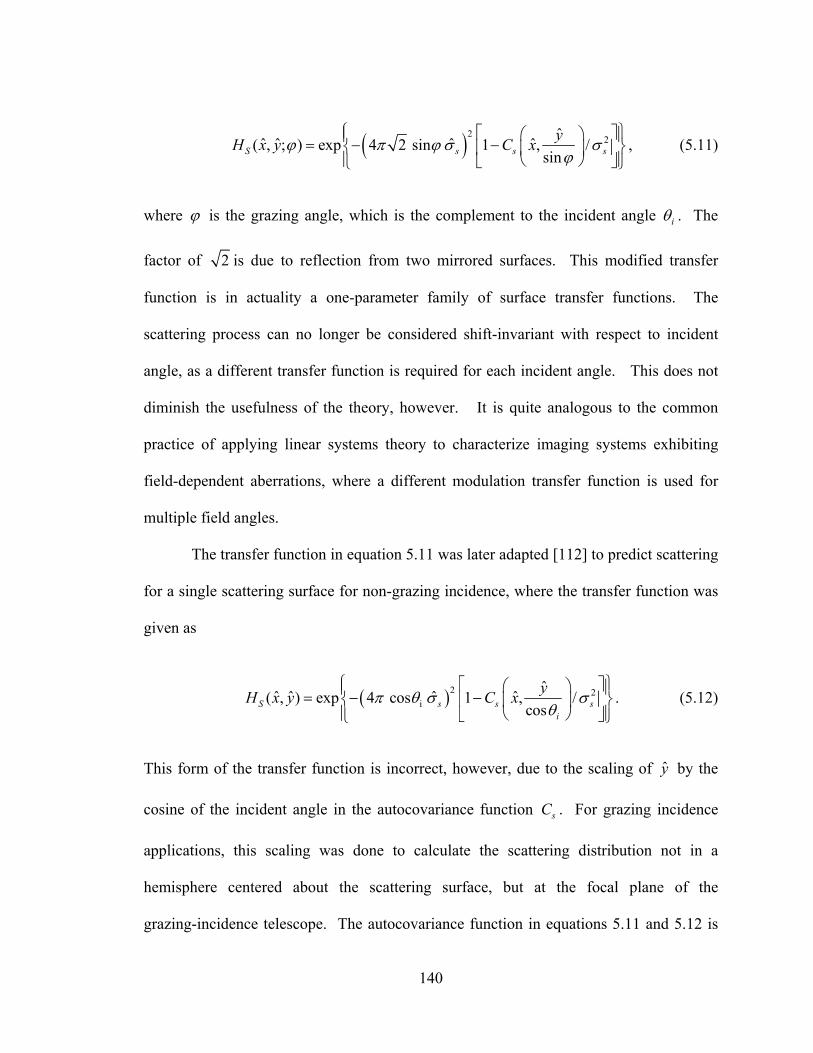
140
( )
2 2ˆˆ ˆ ˆ ˆ( , ; ) exp 4 2 sin 1 , /sinS s s s
yH x y C xϕ π ϕ σ σϕ
⎧ ⎫⎡ ⎤⎛ ⎞⎪ ⎪= − −⎨ ⎬⎢ ⎥⎜ ⎟⎝ ⎠⎪ ⎪⎣ ⎦⎩ ⎭
, (5.11)
where ϕ is the grazing angle, which is the complement to the incident angle iθ . The
factor of 2 is due to reflection from two mirrored surfaces. This modified transfer
function is in actuality a one-parameter family of surface transfer functions. The
scattering process can no longer be considered shift-invariant with respect to incident
angle, as a different transfer function is required for each incident angle. This does not
diminish the usefulness of the theory, however. It is quite analogous to the common
practice of applying linear systems theory to characterize imaging systems exhibiting
field-dependent aberrations, where a different modulation transfer function is used for
multiple field angles.
The transfer function in equation 5.11 was later adapted [112] to predict scattering
for a single scattering surface for non-grazing incidence, where the transfer function was
given as
( ) 2 2
iˆˆ ˆ ˆ ˆ( , ) exp 4 cos 1 , /
cosS s s si
yH x y C xπ θ σ σθ
⎧ ⎫⎡ ⎤⎛ ⎞⎪ ⎪= − −⎨ ⎬⎢ ⎥⎜ ⎟⎝ ⎠⎪ ⎪⎣ ⎦⎩ ⎭
. (5.12)
This form of the transfer function is incorrect, however, due to the scaling of y by the
cosine of the incident angle in the autocovariance function sC . For grazing incidence
applications, this scaling was done to calculate the scattering distribution not in a
hemisphere centered about the scattering surface, but at the focal plane of the
grazing-incidence telescope. The autocovariance function in equations 5.11 and 5.12 is

141
not given in terms of the coordinates of the scattering surface, but in a rotated coordinate
system where ˆ ˆ ˆ ˆ and / cos ox x y y θ= = . For the usual scattering geometry, the correct
form of the modified transfer function for an arbitrary incident angle is therefore given by
( ) ( ){ } 2 2
iˆ ˆ ˆ ˆ ˆ( , ) exp 4 cos 1 , /S s s sH x y C x yπ θ σ σ⎡ ⎤= − −⎣ ⎦ . (5.13)
This can again be written in the form
( )ˆ ˆ ˆ ˆ( , ) ,SH x y A B G x y= + , (5.14)
where ( )2ˆexp 4 cos i sA π θ σ⎡ ⎤= −⎣ ⎦ , (5.15)
( )2ˆ1 exp 4 cos i sB π θ σ⎡ ⎤= − −⎣ ⎦ , (5.16)
and ( )
( )
2
2
ˆ ˆ ˆexp 4 cos ( , ) 1ˆ ˆ( , )
ˆexp 4 cos 1
i
i s
C x yG x y
π θ
π θ σ
⎡ ⎤ −⎣ ⎦=⎡ ⎤ −⎣ ⎦
. (5.17)
A wavefront incident on the scattering surface at an angle iθ is equivalent to
introducing a linear phase shift across the pupil. Assuming the plane of incidence to be
the x-z plane, this will cause a shift of the scattering function in direction cosine space of
oα α− , where sino oα θ= . The ASF is therefore given by the Fourier transform of the
transfer function in equation 5.13 (or 5.14) multiplied by the linear phase shift:
( ) ( ) ( ){ } ( ) ( )ˆ ˆ ˆ, , exp 2 , ,S o o oASF H x y i x A Sα β πα δ α α β α α β= − = − + −F . (5.18)

142
where ( ) ( ) ( ){ }ˆ ˆ ˆ, , exp 2o oS B G x y i xα α β πα− = −F . (5.19)
This is again the sum of a delta function at the location of the specular direction
surrounded by a scattering function, S, where the total power in the specular reflection is
given by A, the percentage of total power in the scattering function (TIS) is given by B,
and A + B = 1.
If any portion of the scattering function S in equation 5.18 falls outside of the unit
circle in direction cosine space, it will need to be truncated and renormalized to account
for conservation of energy. This is accomplished in the same manner as was done for
diffraction in section 3.3 of chapter three. Similar to equation 3.29, the renormalization
constant, K, for the scattering function is given by
( )
( )2
2
1 1-
1 1-
ASF ,
ASF ,
d d
K
d d
βαα
α β α
α β α β
α β α β
∞ ∞
= −∞= −∞
=− = −
=∫ ∫
∫ ∫
. (5.20)
The numerator in equation 5.20 is simply equal to unity, however. The normalization
constant can therefore be written as
( )2
2
1 1-
1 1-
1
ASF ,
K
d dα
α β α
α β α β=− = −
=
∫ ∫, (5.21)
and the angle spread function is then given by
( ) ( ) ( ){ }ˆ ˆ ˆ, , exp 2S oASF K H x y i xα β πα′ = −F . (5.22)

143
Recall from section 2.2.4 that the ASF is a normalized radiance function. We can
therefore convert the angle spread function to intensity by using equation 2.96. The
scattered intensity is therefore given by
( ) ( ) s, , cosiI P ASFα β α β θ= . (5.23)
5.2.1 Smooth Surface Approximation
We will now compare the original and modified Harvey-Shack theories to each
other and with the well-established Rayleigh-Rice theory for smooth surfaces. Although
it is not necessary, it will be useful to make a smooth surface approximation to the
Harvey-Shack theories to aid in the comparison.
A smooth surface implies that the roughness is small compared to the wavelength
of light. If we let ˆ sσ λ<< in equations 5.3-5.5 for the original Harvey-Shack theory, we
obtain
[ ]2ˆ1 4 sA πσ≈ − , (5.24)
[ ]2ˆ4 sB πσ≈ , (5.25)
and ( ) ( ) 2ˆ ˆ ˆ ˆ, , /s sG x y C x y σ= . (5.26)
Using equation 5.7, the scattering function is then given by
( ) ( ){ }2
2
16 ˆ ˆ, ,sS C x yπα βλ
= F . (5.27)

144
After a change of variables from ( )ˆ ˆ,x y to ( ),x y , and recognizing that the autocovariance
function sC and the surface power spectral density (PSD) constitute a Fourier transform
pair, the scattering function can be written in terms of scattering angles as
( ) ( )2
4
16, ; ,OHS s s i x yS PSD f fπθ φ θλ
= , (5.28)
where sin cos sin sin sin, s s i s sx yf fθ φ θ θ φ
λ λ−
= = . (5.29)
From equation 5.23 the scattered intensity for the original Harvey-Shack (OHS) theory is
therefore given by
( ) ( )2
4
16, ; cos ,OHS s s i i s x yI P PSD f fπθ φ θ θλ
⎛ ⎞= ⎜ ⎟
⎝ ⎠. (5.30)
Similarly, the intensity for the modified Harvey-Shack (MHS) theory for smooth surfaces
is given by
( ) ( )2
24
16, ; cos cos ,MHS s s i i s x yiI P PSD f fπθ φ θ θ θ
λ⎛ ⎞
= ⎜ ⎟⎝ ⎠
. (5.31)
Recall from equation 2.39 that the intensity (normalized by incident power) for the
Rayleigh-Rice (RR) theory, assuming a perfect conducting surface and TE polarization,
is given by
( ) ( )2
24
16, ; cos cos ,RR s s i i i s x yI P PSD f fπθ φ θ θ θλ
⎛ ⎞= ⎜ ⎟
⎝ ⎠. (5.32)

145
Comparing equation 5.30 with 5.31, we can see that the original Harvey-Shack
and the modified Harvey-Shack theories are only strictly equal for normal incidence.
They should give similar results, however, for paraxial incident angles when cos 1iθ ≈ .
Comparing both versions of the Harvey-Shack theory to the Rayleigh-Rice theory, we
can see that all three should agree fairly well when both the incident and scattering angles
are paraxial, for which cos ,cos 1i sθ θ ≈ . For larger incident angles, the original
Harvey-Shack will predict both a higher peak and larger TIS than either the modified
Harvey-Shack or the Rayleigh-Rice theories. For all incident angles, the modified
Harvey-Shack and Rayleigh-Rice theories are equal at the location of specular reflection
where cos cosi sθ θ= . They should agree fairly well elsewhere provided that the spread
of the scattering function around the specular beam is small.
For comparison purposes, we will assume the scattering surface to have a
Gaussian autocovariance function of the form
( )2 2
22, exps s
c
x yC x y σ⎡ ⎤+
= −⎢ ⎥⎣ ⎦
. (5.33)
The PSD is then given by
( ) ( )2 2 2 2 2 2, expx y s c c x yPSD f f f fπσ π⎡ ⎤= − +⎣ ⎦ , (5.34)
where lc is the correlation length, and ,x yf f are given by equation 5.29. To calculate the
intensity for the three theories, equation 5.34 is substituted into equations 5.30, 5.31, and
5.32. For smooth surfaces, the RMS roughness only affects the magnitude of the

146
scattering function, not its shape. Therefore we will only use one roughness scale,
/ 0.02sσ λ = , when calculating scatter for smooth surfaces.
Figure 5-2 shows a comparison of the original and modified Harvey-Shack
theories with the Rayleigh-Rice theory for a surface with the autocovariance function
given in equation 5.33. The incident angle is zero degrees and the ratio of the correlation
length to the wavelength of light (lc/λ) is five. The original and modified Harvey-Shack
theories are exactly equal for normal incidence as discussed above. The ratio of lc/λ
determines the angular spread of the scattering function and, in the case of Figure 5-2, the
spread is narrow enough that the Harvey-Shack theories and Rayleigh-Rice theories yield
virtually identical results.
Figure 5-2: OHS and MHS compared to RR for θi = 0° and lc/λ = 5
θi = 0° σs/λ = 0.2 lc/λ = 5

147
In Figure 5-3, the incident angle is again zero degrees, but lc/λ has been decreased
by a factor of ten to 0.5. This results in a much wider angular spread of the scattering
function than in Figure 5-2, and the Harvey-Shack theories depart from the Rayleigh-
Rice theory at larger scattering angles. The original and modified Harvey-Shack theories
still yield identical results since the light is normally incident on the scattering surface.
Figure 5-3: OHS and MHS compared to RR for θi = 0° and lc/λ = 0.5
In Figure 5-4, lc/λ has again been set to five, resulting in a small angular spread of
the scattering function. The incident angle has been increased slightly to five degrees.
θi = 0° σs/λ = 0.02 lc/λ = 0.5

148
The agreement between the three theories is still good; however the original Harvey-
Shack theory deviates slightly from the other two theories near the location of the
specular reflection.
Figure 5-4: OHS and MHS compared to RR for θi = 5° and lc/λ = 5
In Figure 5-5, lc/λ has been kept at five, but the incident angle has been increased
to 40 degrees. The agreement between the modified Harvey-Shack and Rayleigh-Rice
theories is still generally good. The original Harvey-Shack theory departs drastically
from the other two theories. From equation 5.25, the original Harvey-Shack theory
θi = 5° σs/λ = 0.02 lc/λ = 5

149
predicts that 6.32% of the total energy is contained in the scattering function, while both
the modified Harvey-Shack and Rayleigh-Rice theories predict that the scattering
function contains 3.71% of the total energy. The departure will only get worse with
increasing incident angle, as the original Harvey-Shack theory will continue to predict a
TIS of 6.32%, regardless of what the incident angle is, while the TIS predicted by the
modified Harvey-Shack and Rayleigh-Rice theories will continue to decrease with
increasing incident angle.
Figure 5-5: OHS and MHS compared to RR for θi = 40° and and lc/λ = 5
θi = 40° σs/λ = 0.02 lc/λ = 5

150
The modified Harvey-Shack theory is obviously a large improvement over the
original Harvey-Shack theory whenever the incident angle is not small. Therefore, we
will continue to compare only the modified Harvey-Shack theory with the Rayleigh-Rice
theory. In Figures 5-6, 5-7, and 5-8 the two theories are compared for incident angles of
20, 50, and 70 degrees and lc/λ ratios of 1, 5, 10, and 40.
For an incident angle of 20 degrees in Figure 5-6, the only significant departure of
the modified Harvey-Shack theory from the Rayleigh-Rice theory occurs for lc/λ = 1,
when the angular spread of the scattering function is almost 80 degrees. Even then, the
departure is not severe.
For an incident angle of 50 degrees in Figure 5-7, the modified Harvey-Shack
theory departs slightly from the Rayleigh-Rice theory for lc/λ = 5, where the scattering
function is roughly 20 degrees wide. For lc/λ = 1, the departure is quite severe.
In Figure 5-8, where the incident angle is 70 degrees, there is only good
agreement between the two theories when lc/λ = 40, where the width of the scattering
function is about 6 degrees. For all of the other lc/λ ratios, the modified Harvey-Shack
theory departs significantly from the Rayleigh-Rice theory.
The two theories should agree when the angular spread of the scattering function
is small. For small incident angles, the modified Harvey-Shack theory is fairly accurate
even for very wide scattering functions. The restriction on the angular spread becomes
more severe with increasing incident angle, however, and for a given surface, the theory
may work well for smaller incident angles but may break down at larger incident angles.

151
Figure 5-6: MHS compared to RR for θi = 20° and lc/λ = 40, 10, 5, and 1
θi = 20° σs/λ = 0.02 lc/λ = 40
θi = 20° σs/λ = 0.02 lc/λ = 10
θi = 20° σs/λ = 0.02 lc/λ = 5
θi = 20° σs/λ = 0.02 lc/λ = 1

152
Figure 5-7: MHS compared to RR for θi = 50° and lc/λ = 40, 10, 5, and 1
θi = 50° σs/λ = 0.02 lc/λ = 40
θi = 50° σs/λ = 0.02 lc/λ = 10
θi = 50° σs/λ = 0.02 lc/λ = 5
θi = 50° σs/λ = 0.02 lc/λ = 1

153
Figure 5-8: MHS compared to RR for θi = 70° and lc/λ = 40, 10, 5, and 1
θi = 70° σs/λ = 0.02 lc/λ = 40
θi = 70° σs/λ = 0.02 lc/λ = 10
θi = 70° σs/λ = 0.02 lc/λ = 5
θi = 70° σs/λ = 0.02 lc/λ = 1

154
5.2.2 Rough Surfaces
For rough surfaces, a numerical solution to equation 5.18 (or 5.22) will most
likely be required. This is easily accomplished with computational software, such as
MATLAB®, which is what we will use to perform the calculations using the built-in FFT
routine.
Given the ACV function of a surface, as well as the wavelength of light, the
surface transfer function of equation 5.13 or 5.14 is calculated first. If the ACV of the
surface is not known, but the PSD is, the ACV can be calculated from the PSD since the
two constitute a Fourier transform pair. Care must be taken, however, since the PSD is
usually known only over some band-limited region. Fitting the PSD to some functional
form can be useful in these cases to allow extrapolation beyond the known portion of the
PSD.
Figure 5-9 shows the surface transfer function for the O’Donnell-Mendez surface
[110] discussed in chapter four. In this case λ = 10.6 μm, θi = 70°, σs = 2.27 μm, and
lc = 20.9 μm. As seen in the figure, the transfer function consists of the sum of a constant
and a bell-shaped function.
We next use equation 5.18 to calculate the angle spread function which is shown
in Figure 5-10. The constant portion of Figure 5-9 will Fourier transform into a delta
function in the location of specular reflection, while the bell-shaped function will Fourier
transform into the scattering function. The peak of the transfer function is unity, and
therefore from the central ordinate theorem of Fourier transform theory [1], the volume

155
Figure 5-9: MHS surface transfer function for a scattering surface with a Gaussian ACV function. λ = 10.6 μm, θi = 70°, σs = 2.27 μm, lc = 20.9 μm.
Figure 5-10: The ASF calculated by taking the Fourier transform of the transfer function in Figure 5-9

156
under its Fourier transform (the ASF) will also be unity. The constant portion of the
transfer function determines the percentage of the total power that resides in the specular
portion of the ASF, given by A in equation 5.15. The percentage of the total power in the
scattering function is then given by B = 1 – A. For this specific case, B = 0.571.
Any portion of the ASF that falls outside of the unit circle in direction cosine
space is not real and does not propagate. The ASF then needs to be truncated at the unit
circle and renormalized according to equations 5.21 and 5.22. This renormalization
redistributes the energy from that portion of the scattering function that falls outside the
unit circle back into both the real part of the scattering function and the specularly
reflected light. Figure 5-11 shows the result of this truncation and renormalization for the
ASF of Figure 5-10. For this situation, the renormalization factor K is equal to 1.244.
Figure 5-11: Truncated and renormalized ASF of Figure 5-10

157
Figure 5-12 shows a profile of the diffusely scattered portion of the ASF along the
plane of incidence both before and after the truncation and renormalization is performed.
The specular reflection has been omitted. The two profiles differ in magnitude by a
factor of K = 1.244, as calculated from equation 5.21 When plotted as a function of
direction cosines, the scattering function as predicted by the modified Harvey-Shack
theory is symmetrical about the location of specular reflection.
Figure 5-12: Plane-of-incidence profile of the diffusely scattered portion of the ASF in Figure 5-10 both before and after renormalization.

158
The scattered intensity can be calculated from the ASF using equation 5.23.
Figure 5-13 shows a profile of the scattered intensity in the plane-of-incidence as a
function of scattering angle for the diffusely scattered portion of the ASF of Figure 5-10.
The scattered intensity is highly asymmetrical about the direction of specular reflection,
and the peak of the scattered intensity is shifted inside of the specular reflection. The
shift is due to the multiplication of the radiance by a cosine of the scattering angle to
convert it to intensity. The asymmetry is due to both the cosine and the fact that it is
plotted as a function of scattering angle instead of the direction cosine of that angle.
Figure 5-13: Scattered intensity in the plane of incidence as a function of scattering angle for the diffusely scattered portion of the ASF of Figure 5-10

159
A comparison of scattered intensity predicted by the original and modified
Harvey-Shack theories is shown in Figure 5-14 for the O’Donnell-Mendez surface with a
wavelength of 10.6 μm at incident angles of 0, 20, 50, and 70 degrees. Experimental data
taken from [110] for 20 and 70 degrees is also plotted for comparison. For incident
radiation with a wavelength of 10.6 μm, σs/λ = 0.214, and this surface can be considered
moderately rough. Since we only know the profile of the scattered intensity from the
experimental data, we are not able to calculate its volume to scale it to the theoretical
predictions. The peak of the experimental data was therefore normalized to the peak of
the modified Harvey-Shack prediction.
For normal incidence in Figure 5-14, the original and modified Harvey-Shack
theories give the same result. This will always be the case, regardless of how rough the
surface is. For normally incident 10.6 μm radiation, both theories predict that all of the
light will be diffusely scattered, and there will therefore be no specular reflection.
For a 20 degree incident angle, both theories still predict that all of the light will
be diffusely scattered. The original Harvey-Shack theory predicts a smaller peak and a
slightly wider scattering function. The modified Harvey-Shack theory gives a fairly good
fit to the experimental data for this small incident angle, even though the scattering
function has an angular spread of roughly 80 degrees.
For a 50 degree incident angle, the disagreement between the theories is far more
pronounced. The peak of the original Harvey-Shack prediction is about half of the
modified Harvey-Shack peak, and the angular spread is larger. In addition, the original
Harvey-Shack theory still predicts a TIS of 1, while the TIS from the modified
Harvey-Shack theory drops slightly to 0.942.

160
Figure 5-14: MHS compared to OHS and OM experimental data for σs/λ = 0.214, lc/λ = 1.97, and θi = 0°, 20°, 50°, and 70°
θi = 0° σs/λ = 0.214 lc/λ = 1.97 TISOHS = 1 TISMHS = 1
θi = 20° σs/λ = 0.214 lc/λ = 1.97 TISOHS = 1 TISMHS = 1
θi = 50° σs/λ = 0.214 lc/λ = 1.97 TISOHS = 1 TISMHS = 0.94
θi = 70° σs/λ = 0.214 lc/λ = 1.97 TISOHS = 1 TISMHS = 0.47

161
For the 70 degree incident angle in Figure 5-14, the disagreement between the
original and modified Harvey-Shack theories is worse still. The peak of the original
theory is once again smaller than the modified theory, and the angular spread wider. In
addition, while both theories predict that the peak of the scattering function is shifted
from the specular direction, the original theory predicts a larger shift. Even more
significant is that the original Harvey-Shack theory continues to predict that all of the
light will be diffusely scattered, while the modified Harvey-Shack theory predicts that the
TIS will drop to 0.465 for this incident angle. Comparing the theories with the
experimental data, it is once again obvious that the modified Harvey-Shack theory is a
vast improvement over the original theory, especially at large incident angles. Even so,
the agreement of the modified theory with the experimental data is far from ideal. This is
understandable, however, as it can not be expected to work well with such wide angle
scattering at large incident angles.
In Figure 5-15, we are once again comparing the original and modified
Harvey-Shack theories with experimental data for the O’Donnell-Mendez surface, this
time for visible light at 0.6328 μm. At this wavelength, σs/λ = 3.59, and the surface can
be considered very rough. Both the original and modified theories predict that all of the
light will be diffusely scattered, with no specular reflection. The disagreement between
the theories is once again quite severe, however, with the original theory having a much
smaller peak and a much larger angular spread. The modified theory may be an
improvement, but its agreement with the data is still not very good. The peak of the
modified theory is once again shifted inside of the specular direction, but in this case the
data does not exhibit the same shift. The slope of the scattering function in the

162
backwards scattering direction is also much steeper for the modified Harvey-Shack
prediction than it is for the experimental data. Once again, the inaccuracy of the theory
should not be surprising, since the assumption of small angle scattering has been violated.
Figure 5-15: MHS compared to OHS and OM experimental data for σs/λ = 3.59, lc/λ = 33.0, and θi = 70°
5.3 The Generalized Harvey-Shack Formulation
The modified version of the Harvey-Shack theory was clearly an improvement
over the original Harvey-Shack theory, especially for anything larger than paraxial
incident angles. However, the restriction of small angular spread of the scattering
function, which becomes more stringent at large incident angles, is very limiting. We
θi = 70° σs/λ = 3.59 lc/λ = 33.0 TISOHS = 1 TISMHS = 1

163
will remove this limitation in the following development by generalizing the
Harvey-Shack theory for large incident and scattering angles.
Figure 5-16 illustrates radiation incident on a scattering surface at an arbitrary
incident angle, θi. It is obvious from examining the figure that the optical path difference
introduced upon reflection depends not just on the surface height and incident (and
specular) angle, but also on the scattering angle θs. The OPD can be written as
( ) ( ) ˆ ˆcos cos , ;0i sOPD h x yθ θ= + . (5.35)
h
θi
θs
x∧
Sur
face
Hei
ght
h
θi
θs
x∧x∧
Sur
face
Hei
ght
Figure 5-16: Illustration of the OPD for a ray scattered at an arbitrary angle θs
The random phase variation of the reflected wavefront can therefore be written as
( ) ( ) ( ) ( ) ˆˆ ˆ ˆ ˆ, 2 / 2 , ;0i sx y OPD h x yφ π λ π γ γ= = + , (5.36)

164
where cos and cosi i s sγ θ γ θ= = . (5.37)
If we return to the derivation of the original Harvey-Shack theory which was
summarized in chapter two, we can use equation 5.36 to rewrite the random component
of the pupil function given by equation 2.97 as
( ) ( ) ( ) ( )ˆˆ ˆ ˆ ˆ ˆ ˆ, ;0 , ;0 exp 2 , ;0R s i sP x y a x y i h x yπ γ γ⎡ ⎤= +⎣ ⎦ . (5.38)
Substituting equation 5.38 into equation 2.97, and completing the derivation as before
results in a surface transfer function given by
( ) ( ) ( ){ }
2 2ˆ ˆ ˆ ˆ ˆ, ; , exp 2 1 , /S i s s i s s sH x y C x yγ γ π σ γ γ σ⎡ ⎤⎡ ⎤= − + −⎣ ⎦ ⎣ ⎦ . (5.39)
This generalized Harvey-Shack transfer function is in reality a two-parameter family of
surface transfer functions. A different transfer function is required for each incident and
scattering angle. The angle spread function is given by
( ) ( ) ( ){ } ,ˆ ˆ ˆ, , ; , exp 2s s S i s o s s
ASF H x y i xα α β β
α β γ γ πα= =
= −F . (5.40)
Equation 5.40 corresponds to the light scattered in the αs, βs direction. The direction
cosines αs and βs are related to γs by
2 21s s sγ α β= − − . (5.41)
As before, the surface transfer function can be written in the form
( ) ( )ˆ ˆ ˆ ˆ, ; , , ; ,S i s i sH x y A B G x yγ γ γ γ= + , (5.42)

165
where ( ){ }2ˆexp 2 i s sA π γ γ σ⎡ ⎤= − +⎣ ⎦ , (5.43)
( ){ }2ˆ1 exp 2 i s sB π γ γ σ⎡ ⎤= − − +⎣ ⎦ , (5.44)
and ( ) ( ){ }
( )
2
2
ˆ ˆ ˆexp 2 , 1ˆ ˆ( , ; , )
ˆexp 2 1
i s
i s
i s s
C x yG x y
π γ γγ γ
π γ γ σ
⎡ ⎤+ −⎣ ⎦=
⎡ ⎤+ −⎣ ⎦. (5.45)
The ASF can then be written as
( ) ( ) ( ) ,, , ,s s o o s s
ASF A Sα α β β
α β δ α α β α α β= =
⎡ ⎤= − + −⎣ ⎦ , (5.46)
where ( ) ( ) ( ){ }ˆ ˆ ˆ, , ; , exp 2o i s oS B G x y i xα α β γ γ πα− = −F . (5.47)
Equations 5.40 and 5.46 indicate that for a given incident angle, a different
Fourier transform needs to be performed in order to calculate the ASF for each scattering
angle. This process can be avoided if the Fourier transform can be solved analytically.
When this is the case, γs is just treated as a constant since it is not a function of the
variables of integration ˆ ˆ and x y . When a numerical solution is required, multiple
transforms will indeed have to be performed in order to calculate the entire angle spread
function.
Since the delta function in equation 5.46 is equal to zero except when oα α= ,
equation 5.43 corresponds to the percentage of the total power that resides in the
specularly reflected light when i sγ γ= . A is then given by

166
[ ]{ }2ˆexp 4 i sA πγ σ= − . (5.48)
This is the same value predicted by the modified Harvey-Shack theory. The percentage
of the total power that is diffusely scattered is therefore given by
[ ]{ }2ˆ1 1 exp 4 i sB A πγ σ= − = − − . (5.49)
Once the ASF is known over the entire observation hemisphere, equation 5.21 can be
used to renormalize the ASF to unit volume and thus ensure conservation of energy.
5.3.1 Smooth Surface Approximation
For smooth surfaces, we will compare the predictions of the generalized
Harvey-Shack theory to both the modified Harvey-Shack theory and the well-established
Rayleigh-Rice scattering theory. When the roughness of a surface is small compared to
the wavelength of incident light, we can again make an approximation to the surface
transfer function. Letting ˆ sσ λ<< in equations 5.43-5.45 yields
( ) 2ˆ1 2 s i sA πσ γ γ⎡ ⎤≈ − +⎣ ⎦ , (5.50)
( ) 2ˆ2 s i sB πσ γ γ⎡ ⎤≈ +⎣ ⎦ , (5.51)
and ( ) ( ) 2ˆ ˆ ˆ ˆ, , /s sG x y C x y σ= . (5.52)
Using equation 5.47, the scattering function can be written as

167
( ) ( ) ( ){ }2
2i2
4 ˆ ˆ, ,s sS C x yπα β γ γλ
= + F . (5.53)
Writing this in integral form gives
( ) ( ) ( ) ( )2
2i2
- -
4 ˆ ˆ ˆ ˆ ˆ ˆ, , exp 2s sS C x y i x y dxdyπα β γ γ π α βλ
∞ ∞
∞ ∞
⎡ ⎤= + − +⎣ ⎦∫ ∫ . (5.54)
Performing a change of variables from ( ) ( )ˆ ˆ, to ,x y x y yields
( ) ( ) ( ) ( )2
2i2 2
- -
4 1, , exp 2s s x yS C x y i f x f y dxdyπα β γ γ πλ λ
∞ ∞
∞ ∞
⎡ ⎤= + − +⎣ ⎦∫ ∫ . (5.55)
The integral in 5.55 is the Fourier transform of the autocovariance function ( ),sC x y ,
which is simply the power spectral density of the surface. The scattering function for the
generalized Harvey-Shack (GHS) theory can therefore be written in terms of spherical
angles as
( ) ( ) ( )2
24
4, ; cos cos PSD ,GHS s s i i s x yS f fπθ φ θ θ θλ
= + , (5.56)
where from the grating equation
sin cos sin sin sin, s s i s sx yf fθ φ θ θ φ
λ λ−
= = . (5.57)
Using equation 5.23, we can write the diffusely scattered intensity as
( ) ( ) ( )2
2s4
4, ; cos cos cos PSD ,GHS s s i i i s x yI P f fπθ φ θ θ θ θλ
= + . (5.58)

168
Recall from equation 5.31 that the scattered intensity predicted by the modified
Harvey-Shack (MHS) theory for a perfectly conducting smooth surface is given by
( ) ( )2
24
16, ; cos cos ,MHS s s i i i s x yI P PSD f fπθ φ θ θ θλ
⎛ ⎞= ⎜ ⎟
⎝ ⎠, (5.59)
and from equation 5.32 the scattered intensity predicted by the Rayleigh-Rice (RR)
theory for a perfectly conducting smooth surface and TE polarization is given by
( ) ( )2
24
16, ; cos cos ,RR s s i i i s x yI P PSD f fπθ φ θ θ θλ
⎛ ⎞= ⎜ ⎟
⎝ ⎠. (5.60)
Comparing equations 5.58, 5.59, and 5.60 we can see that all three equations are
approximately equal for small incident and scattering angles when cos cos 1i sθ θ≈ ≈ . All
three equations should be exactly equal when s iθ θ= , or when s oθ θ= since
cos cosi oθ θ= .
To compare the modified and generalized Harvey-Shack theories with the
Rayleigh-Rice theory, we will again assume a scattering surface with the Gaussian
autocovariance function in equation 5.33. The PSD is then given by equation 5.34. The
ratio of the RMS surface roughness to the wavelength will again be assumed to be 0.02.
Figure 5-17 shows a comparison of the three theories for normal incidence and an
lc/λ ratio of five. The angular spread of the scattering function is less than 20 degrees
wide, which for normal incidence is relatively small. For this set of parameters, all three
theories yield virtually identical results.

169
Figure 5-17: GHS and MHS compared to RR for θi = 0° and lc/λ = 5
In Figure 5-18, the angle of incidence has been kept at 0 degrees, but the ratio of
lc/λ has been decreased by a factor of ten to 0.5. This results in a much larger angular
spread of the scattering function, and the modified Harvey-Shack theory departs from the
Rayleigh-Rice prediction at larger scattering angles. The generalized Harvey-Shack
theory, however, agrees quite well with the Rayleigh-Rice theory even at large scattering
angles.
In Figures 5-19, 5-20, and 5-21, the modified Harvey-Shack, generalized Harvey-
Shack, and Rayleigh-Rice theories are compared for incident angles of 20, 50, and 70
degrees and lc/λ ratios of 10, 5, 1, and 0.5.
θi = 0° σs/λ = 0.02 lc/λ = 5

170
Figure 5-18: GHS and MHS compared to RR for θi = 0° and lc/λ = 0.5
For the 20 degree incident angle in Figure 5-19, the three theories agree extremely
well for lc/λ = 10 and lc/λ = 5 for which the scattering function is relatively narrow. For
lc/λ = 1 and lc/λ = 0.5, the generalized Harvey-Shack and Rayleigh-Rice theories
continue to agree quite well, while the modified Harvey-Shack theory departs from the
other two. The only noticeable departure of the generalized Harvey-Shack from the
Rayleigh-Rice occurs at the larger negative scattering angles for lc/λ = 0.5, and even this
is relatively minor.
θi = 0° σs/λ = 0.02 lc/λ = 0.5

171
Figure 5-19: GHS and MHS compared to RR for θi = 20° and lc/λ = 10, 5, 1, and 0.5
θi = 20° σs/λ = 0.02 lc/λ = 10
θi = 20° σs/λ = 0.02 lc/λ = 5
θi = 20° σs/λ = 0.02 lc/λ = 1
θi = 20° σs/λ = 0.02 lc/λ = 0.5

172
Figure 5-20: GHS and MHS compared to RR for θi = 50° and lc/λ = 10, 5, 1, and 0.5
θi = 50° σs/λ = 0.02 lc/λ = 1
θi = 50° σs/λ = 0.02 lc/λ = 0.5
θi = 50° σs/λ = 0.02 lc/λ = 5
θi = 50° σs/λ = 0.02 lc/λ = 10

173
Figure 5-21: GHS and MHS compared to RR for θi = 70° and lc/λ = 10, 5, 1, and 0.5
θi = 70° σs/λ = 0.02 lc/λ = 10
θi = 70° σs/λ = 0.02 lc/λ = 1
θi = 70° σs/λ = 0.02 lc/λ = 5
θi = 70° σs/λ = 0.02 lc/λ = 0.5

174
For the 50 degree incident angle in Figure 5-20, the modified Harvey-Shack
theory is just beginning to depart from the other two when lc/λ = 10 and lc/λ = 5. For the
other two lc/λ values, the departure of the modified Harvey-Shack theory is quite drastic.
The generalized Harvey-Shack theory, on the other hand, agrees very well with the
Rayleigh-Rice theory for all values of lc/λ. The only departure again comes for the
larger negative scattering angles for both lc/λ = 1 and lc/λ = 5.
For the 70 degree incident angle in Figure 5-21, the modified Harvey-Shack
theory departs significantly from the other two theories for all values of lc/λ. The
generalized Harvey-Shack theory and Rayleigh-Rice theory agree very well for lc/λ = 10
and lc/λ = 5. For both lc/λ = 1 and lc/λ = 0.5, the two theories depart slightly. The shapes
of the scattering function predicted by both theories are virtually identical; however the
generalized Harvey-Shack result is shifted slightly towards zero degrees. Despite this
discrepancy, the agreement is still quite good.
Most optical surfaces do not have a Gaussian autocovariance function and PSD.
They instead tend to have a PSD with an inverse power law falloff at larger spatial
frequencies. A sufficiently general model for this behavior is the abc or K-correlation
model [46,113] The autocovariance function is given by
( ) ( ) ( )
( )1 / 2/ 21/ 2
( 1) / 22 2 22
/ 2
cc
s ca r rC rb c b b
π ππ−−
−⎛ ⎞ ⎛ ⎞= ⎜ ⎟ ⎜ ⎟Γ ⎝ ⎠ ⎝ ⎠
K , (5.61)
where a, b, and c are fitting parameters, ( 1) / 2C−K is the modified Bessel function of the
second kind [114], and ( )2 2r x y= + . The two-dimensional PSD is the Fourier

175
transform of equation 5.61 and is given by
( ) ( )( ) ( ) ( )1 / 22 2 2
1 / 21,/ 22 1
x y c
x y
c abPSD f fc b f fπ +
⎡ ⎤Γ +⎣ ⎦=Γ ⎡ ⎤+ +⎣ ⎦
. (5.62)
The parameters a and b are usually expressed in units of Å2-μm and μm-1, while the
parameter c is unitless. If c is greater than 1, the PSD will have a finite volume equal to
the square of the RMS roughness given by
( )
( )2 1 / 2
1 / 2s
c ac c b
πσ⎡ ⎤Γ +⎣ ⎦=
− Γ. (5.63)
The intensity predicted by the generalized Harvey-Shack and Rayleigh-Rice
theories for the K-correlation model can be calculated by substituting equation 5.62 into
equations 5.58 and 5.60, respectively. Figure 5-22 shows a comparison of the two
theories for a surface with a K-correlation PSD with a = 1.5E5, b = 300, c = 1.4, and
incident radiation with a wavelength of 0.6328 μm for incident angles of 0, 20, 50, and
70 degrees.
For all four angles of incidence in Figure 5-22, the biggest disagreement between
the two theories occurs at the larger scattering angles. Note however that the intensity is
plotted on a log scale. The majority of the power is contained in near-specular region,
and very little is contained out at the larger angles. The differences between the two
theories are therefore relatively minor, and the agreement can still be considered very
good. This disagreement will be explored further in section 5.3.3 when we discuss the
inverse scattering problem.

176
Figure 5-22: GHS and RR for a K-Correlation PSD with a = 1.5E5, b = 300, c = 1.4, λ = 0.6328μm for θi = 0°, 20°, 50°, and 70°
θi = 0° a = 1.5E5 b=300 c=1.4 λ=0.6328 μm
θi = 20° a = 1.5E5 b=300 c=1.4 λ=0.6328 μm
θi = 50° a = 1.5E5 b=300 c=1.4 λ=0.6328 μm
θi = 70° a = 1.5E5 b=300 c=1.4 λ=0.6328 μm

177
5.3.2 Quasi-Vectorizing The Harvey-Shack Theory For Smooth Surfaces
One of the limitations of the original Harvey-Shack theory is the fact that since it
is a scalar theory, it is unable to account for polarization effects. This is still true for the
generalized Harvey-Shack theory presented in the last section. All of the comparisons we
have made so far have assumed that the scattering surface is perfectly conducting and that
the incident light was TE polarized. The angle spread function was derived to be
independent of any material effects of the scattering surface. The ASF is not a quantity
that can in reality be measured, however. Intensity is the quantity that is actually
measured in practice, and when it is it will include the effects of both material properties
(reflectance) and polarization.
The intensity for a non-perfectly conducting smooth surface as predicted by the
generalized Harvey-Shack theory is given by:
( ) ( ) ( )2
2s4
4, ; cos cos cos PSD ,GHS s s i i i s x yI P R f fπθ φ θ θ θ θλ
= + , (5.64)
where R is the reflectance of the scattering surface. From equation 2.39, the intensity for
the Rayleigh-Rice theory can be written as
( ) ( )2
2s4
16, ; cos cos PSD ,RR s s i i i x yI P Q f fπθ φ θ θ θλ
= , (5.65)
where Q is the polarization dependent reflectance of the surface given by equations 2.44
through 2.52.

178
We have already shown in the previous section that apart from some small
discrepancies at large scattering angles, equations 5.64 and 5.65 give virtually identical
results for perfectly conducting (i.e., R = Q = 1) surfaces and TE polarized radiation.
Therefore, we will quasi-vectorize the generalized Harvey-Shack theory for smooth
surfaces by replacing the reflectance R in equation 5.64 with the polarization dependent
reflectance Q of the Rayleigh-Rice theory. This will then allow us to account for
polarization effects with the generalized Harvey-Shack theory, at least for smooth
surfaces.
5.3.3 Inverse Scattering For Smooth Surfaces
Thus far in this chapter, we have discussed the prediction of surface scatter from
known surface roughness in the form of the power spectral density or autocovariance
function of a surface. It is often desirable to solve the inverse problem: calculation of
surface roughness from scattering measurements. The first attempt at solving the inverse
scattering problem was most likely that of Bennett and Porteus [115] based on the scalar
theory of Davies [2]. The Rayleigh-Rice vector theory is the most widely used method of
performing inverse scattering from smooth surfaces, and has been discussed in detail by
Stover [3].
For smooth, clean, front-surface reflecting surfaces, the PSD of a surface is
related to the scattering BRDF using the Rayleigh-Rice theory by
( ) ( )2
s4
16, ; cos cos PSD ,RR s s i i x yBRDF Q f fπθ φ θ θ θλ
⎛ ⎞= ⎜ ⎟
⎝ ⎠, (5.66)

179
where, once again, and x yf f are related to the incident and scattering angles by
sin cos sin sin sin, s s i s sx yf fθ φ θ θ φ
λ λ−
= = . (5.67)
Using the generalized Harvey-Shack theory, the relationship between the BRDF and the
surface PSD is given by
( ) ( ) ( )2
2s4
4, ; cos +cos PSD ,GHS s s i i x yBRDF Q f fπθ φ θ θ θλ
⎛ ⎞= ⎜ ⎟
⎝ ⎠, (5.68)
where and x yf f are given by equation 5.67, and we have used the polarization-dependent
surface reflectance as discussed in section 5.3.2.
Given a measured BRDF, we can therefore invert equations 5.66 or 5.68 and solve
for the PSD. The PSD determined by this procedure will actually be a bandwidth-limited
portion of the actual surface PSD; the frequency limits will depend on both the
wavelength of light and the incident angle as can be seen from equation 5.67. The
maximum frequency at which the PSD can be determined will increase with increasing
angle of incidence and decreasing wavelength. This is useful in that the PSD calculated
from scattering measurements for a given wavelength and angle of incidence can then be
used to calculate angle-limited scattering from different wavelengths and angles of
incidence. In addition, if the PSD is well behaved, it can be fit with an analytical
function and extrapolated to higher frequencies so that scattering can be calculated for
both larger and smaller wavelengths and angles of incidence.

180
It is important to realize, however, that not all surfaces will scale with wavelength
in the manner described. Some may scale correctly over a limited wavelength region,
while some may not scale correctly at all. Surfaces that do not scale correctly at a certain
wavelength most likely do not meet the requirements of being smooth, clean, and
front-surface reflecting at that wavelength, even though they may meet these
requirements at other wavelengths.
As an example of the inverse scattering process, we will use a measured scattering
BRDF from a molybdenum mirror surface to calculate the surface PSD. We will then use
that PSD to predict the BRDF at different angles of incidence and compare it to
experimental measurements. All of the BRDF and reflectance measurements for this
mirror surface were performed and provided to us by John Stover of The Scatterworks
[116].
The measured BRDF for the molybdenum mirror for an incident angle of −5
degrees, a wavelength of 0.488μm, and TE polarization in the plane of incidence is
shown in Figure 5-23. Note that the sharp drop in the curve occurs when the detector
passes through the incident beam. The BRDF spans several orders of magnitude and is
fairly symmetric about the location of specular reflection.
The reflectance of the molybdenum mirror is shown in Figure 5-24. The
reflectance was measured at three different angles and a polynomial fit to the data was
then performed, with the assumption that the reflectance goes to unity at 90 degrees. The
equation of the polynomial fit is given in the figure.

181
1.E-08
1.E-07
1.E-06
1.E-05
1.E-04
1.E-03
1.E-02
1.E-01
1.E+00
1.E+01
1.E+02
-90 -75 -60 -45 -30 -15 0 15 30 45 60 75 90
Scattering Angle (degrees)
BR
DF
Figure 5-23: Measured BRDF of molybdenum mirror for θi = −5° and λ = 0.488 μm
0.4
0.6
0.8
1.0
0 10 20 30 40 50 60 70 80 90
Angle (Degrees)
Ref
lect
ance
Measured Values
Polynomial Fit
R = 4.45E-13 θ6 + 3.07E-21 θ5 - 4.80E-09 θ4 + 7.01E-16 θ3
+ 6.30E-05 θ2 - 1.36E-11 θ + 5.68E-01
Figure 5-24: Reflectance of the molybdenum mirror as a function of angle

182
The PSD of the mirror can now be calculated from the BRDF in Figure 5-23
through the use of equation 5.66 for the Rayleigh-Rice theory or equation 5.68 for the
generalized Harvey-Shack theory. In order to do so, we need to know the polarization
dependent reflectance, Q. For TE polarized incident radiation and measurement in the
plane of incidence, Q is given by [3]
( ) ( ) ( ),o s o sQ R Rθ θ θ θ= , (5.69)
where ( )oR θ is the reflectance in the specular direction and ( )sR θ is the reflectance in
the scattered direction. These reflectance values can be calculated through the use of the
polynomial equation given in Figure 5-24.
The PSD predicted using equation 5.66 for the Rayleigh-Rice theory is shown in
Figure 5-25, and the generalized Harvey-Shack prediction from equation 5.68 is shown in
Figure 5-26. Both theories predict a PSD that appears linear when plotted on a log-log
scale, and the agreement between the two is excellent up until a frequency of 1 μm-1.
Beyond that point, the Rayleigh-Rice prediction demonstrates a sharp up-turn. The
generalized Harvey-Shack prediction has a very slight up-turn at the end, but it is not
nearly as drastic as that of the Rayleigh-Rice theory. It is possible that this up-turn is due
to particulate scattering, where light scattering off of particles either in the air or on the
surface itself dominates the surface scattering. This does not explain the difference
between the two theories, however. Recall from section 5.3.1 that intensity predictions
for the Rayleigh-Rice and generalized Harvey-Shack theories tend to disagree only at
large scattering angles. This disagreement becomes even more apparent when comparing

183
1.E-01
1.E+00
1.E+01
1.E+02
1.E+03
1.E+04
1.E+05
1.E+06
1.E+07
1.E+08
0.001 0.01 0.1 1 10
Spatial Frequency (μm-1)
PSD
(Å2 - μ
m2 )
Forward Scattered
Backward Scattered
Figure 5-25: Predicted PSD of the molybdenum mirror using the Rayleigh-Rice theory and measured BRDF data for θi = −5° and λ = 0.488 μm
1.E-01
1.E+00
1.E+01
1.E+02
1.E+03
1.E+04
1.E+05
1.E+06
1.E+07
1.E+08
0.001 0.01 0.1 1 10Spatial Frequency (μm-1)
PSD
(Å2 - μ
m2 )
Forward Scattered
Backward Scattered
Figure 5-26: Predicted PSD of the molybdenum mirror using the generalized Harvey-Shack theory and measured BRDF data for θi = −5° and λ = 0.488 μm

184
the BRDFs predicted by the two theories. Figure 5-27 shows predicted BRDFs for a
surface with a K-correlation PSD given by equation 5.62 with a = 1.5E5, b = 300,
c = 1.4, and incident radiation with a wavelength of 0.6328 μm for normal incidence.
The agreement between the two theories is extremely good until approximately ±60
degrees. After that, the Rayleigh-Rice prediction begins dropping sharply to zero, while
the generalized Harvey-Shack maintains a steady rate of decrease and has a non-zero
value at ±90 degrees.
Figure 5-27: GHS and RR predictions of BRDF for a K-Correlation PSD with a = 1.5E5, b = 300, c = 1.4, and λ = 0.6328 μm for normal incidence.
The fact that the BRDF predicted by the Rayleigh-Rice theory drops to zero at
±90 degrees is a direct consequence of the factor cosθs in equation 5.66. The
Rayleigh-Rice theory predicts that all BRDFs go to zero at ±90 degrees. The BRDF is a

185
radiance distribution, and while intensity must tend to zero at ±90 degrees, there is no
requirement that radiance do so. We know, for instance, that the radiance of a
Lambertian surface is a constant as a function of angle, and is therefore discontinuous at
±90 degrees. We are therefore skeptical of the Rayleigh-Rice BRDF prediction at large
scattering angles.
Figure 5-28 again shows the generalized Harvey-Shack prediction of the PSD of
the molybdenum mirror, but with the addition of a K-correlation fit to the predicted PSD.
The parameters of the K-correlation PSD are shown on the figure. We will use this fit to
predict the scattered BRDF for incidence angles of 5, 45, and 75 degrees.
1.E-01
1.E+00
1.E+01
1.E+02
1.E+03
1.E+04
1.E+05
1.E+06
1.E+07
1.E+08
0.001 0.01 0.1 1 10Spatial Frequency (μm-1)
PSD
(Å2 - μ
m2 )
Forward ScatteredBackward ScatteredK-Correlation Fit
Figure 5-28: K-correlation fit to the PSD prediction shown in Figure 5-26

186
Figure 5-29 shows a comparison of the Rayleigh-Rice and generalized
Harvey-Shack BRDF predictions with experimental data for an incident angle of −5
degrees and a wavelength of 0.488 μm. The two theories agree extremely well out to
scattering angles of around 60 degrees. At larger angles, the generalized Harvey-Shack
prediction seems to agree better with the measured data. As previously stated, the BRDF
may be dominated by particulate scattering at large scattering angles, so this agreement
may simply be fortuitous.
1.E-06
1.E-05
1.E-04
1.E-03
1.E-02
1.E-01
1.E+00
1.E+01
1.E+02
-90 -75 -60 -45 -30 -15 0 15 30 45 60 75 90
Scattering Angle (degrees)
BR
DF
GHS PredictionRR PredictionMeasured Data
Figure 5-29: GHS and RR predictions of the BRDF for the molybdenum mirror compared to experimental data for θi = −5° and λ = 0.488

187
Figure 5-30 shows a comparison of the two theories with experimental data for an
incident angle of −45 degrees and a wavelength of 0.488 μm. The two theories agree
extremely well with each other in the backscattered portion of the BRDF, again until
approximately −60 degrees, and both theories agree very well with the data out to −24
degrees, or approximately 70 degrees from the location of specular reflection. Beyond
that, both theories depart from the data, and this again may be due to the domination of
particulate scatter at angles far from the specular direction. This does not explain the
disagreement in the forward direction, however. The data at larger scattering angles in
the forward direction does not tend to zero as predicted by the Rayleigh-Rice theory, but
instead seems to more closely follow the generalized Harvey-Shack prediction.
1.E-07
1.E-06
1.E-05
1.E-04
1.E-03
1.E-02
1.E-01
1.E+00
1.E+01
1.E+02
-90 -75 -60 -45 -30 -15 0 15 30 45 60 75 90
Scattering Angle (degrees)
BR
DF
GHS PredictionRR PredictionMeasured Data
Figure 5-30: GHS and RR predictions of the BRDF for the molybdenum mirror compared to experimental data for θi = −45° and λ = 0.488

188
Figure 5-31 shows a comparison of the two theories with experimental data for an
incident angle of −75 degrees and a wavelength of 0.488 μm. The two theories agree
very well with each other near the specular beam and out to approximately −80 degrees
in the backscattered portion of the BRDF; however there is a discrepancy between the
two theories for angles between −75 and +75 degrees. Comparing equations 5.66 and
5.68, we can see that the two theories are only strictly equal when the scattering angle is
equal to either the incident or specular angle. As the distance between the incident and
specular angle increases, the disagreement between the two theories will increase at
points in between those two angles. The two theories agree well with the data between
15 and 80 degrees, but they again disagree substantially at large negative scattering
angles. Once again, this may be due to the dominance of particulate scatter.
1.E-08
1.E-07
1.E-06
1.E-05
1.E-04
1.E-03
1.E-02
1.E-01
1.E+00
1.E+01
1.E+02
-90 -75 -60 -45 -30 -15 0 15 30 45 60 75 90
Scattering Angle (degrees)
BR
DF
GHS PredictionRR PredictionMeasured Data
Figure 5-31: GHS and RR predictions of the BRDF for the molybdenum mirror compared to experimental data for θi = −75° and λ = 0.488

189
5.3.4 Numerical Calculations For Rough Surfaces
When the roughness of a scattering surface is not small compared to the
wavelength of the incident radiation, we cannot use the approximations of section 5.3.1.
If no other approximations can be made that will result in an analytical solution of
equation 5.40, numerical methods will be required to compute the scattered light
distribution.
Recall that the surface transfer function for the generalized Harvey-Shack theory
is given by
( ) ( ) ( ){ }
2 2ˆ ˆ ˆ ˆ ˆ, ; , exp 2 1 , /S i s s i s s sH x y C x yγ γ π σ γ γ σ⎡ ⎤⎡ ⎤= − + −⎣ ⎦ ⎣ ⎦ , (5.70)
where 2 2cos and 1 cosi i s s s sγ θ γ α β θ= = − − = . (5.71)
The angle spread function, which consists of both the specular reflection and the diffusely
scattered light distribution, is given by
( ) ( ) ( ){ } ,ˆ ˆ ˆ, , ; , exp 2s s S i s o s s
ASF H x y i xα α β β
α β γ γ πα= =
= −F , (5.72)
where ( )2 2ssin and 1o o s sα θ γ α β= = − + . (5.73)
When numerical solutions of equation 5.72 are required, the parameters iγ and sγ
have to be specified before performing the Fourier transform. Calculating the scattering
distribution over the entire observation space for a given angle of incidence will therefore

190
require a different transfer function and Fourier transform calculation for every scattering
angle.
Direction cosine space is a very convenient space in which to perform the
necessary calculations, as the entire observation hemisphere can be reduced to a circle
with unit radius in the α, β plane. Figure 5-32 shows a grid of discreet values in the α, β
plane along with the unit circle representing all space. This unit circle corresponds to
90sθ = for all values of sφ in the spherical coordinate system.
Figure 5-32: Grid of α, β values with unit circle representing the observation space
αk2 + βj
2 = 1
αk
βj

191
It is straightforward to create a grid like the one shown in Figure 5-32 in
MATLAB® as a two dimensional array and then perform the calculation of the ASF,
given by equation 5.72, for each point in the array. For points that lie outside of the unit
circle, we can simply assign a value of zero to the ASF, since γs is not a real number at
those locations. The calculation of the entire ASF can be written as
( ) ( ), ,jk k jj k
ASF K ASFα β α β= ∑∑ , (5.74)
where ( ) ( ) ( ){ } ,ˆ ˆ ˆ, , ; , exp 2k j s i jk o
s s jkASF H x y i x
α α β βα β γ γ πα
= == F , (5.75)
2 21jk k jγ α β= − − , (5.76)
and K is the renormalization constant given by equation 5.21.
As an example of the process, we will calculate the scattering of the
O’Donnell-Mendez surface discussed previously. The Gaussian autocovariance function
of this surface is given by equation 5.33 with σs = 2.27 μm and lc = 20.9 μm. We will
assume that the incident radiation has a wavelength 10.6 μm, and that the angle of
incidence is 45 degrees ( )2 / 2, 2 / 2o iα γ= − = .
We first set up a two-dimensional square array of size N 2 for the ASF. Each array
location corresponds to points in the α, β plane, where α and β are one-dimensional
arrays of length N; α varies from -1 to 1, while β varies from 1 to -1. The first location in
the ASF array (j = 1, k = 1) corresponds to α = −1, β = 1. The last location in the ASF
array (j = N, k = N) corresponds to α = 1, β = -1.

192
We will let N=101, so that the ASF is a square array of 101 x 101 locations. We
first set k = 1, which corresponds to α = −1, and we set j = 1 which corresponds to β = 1.
For these values, γjk is a complex number since that location lies outside of the unit circle.
We therefore assign a value of zero to the ASF at that location. We then continue to loop
through values of j and k. At each step we calculate equation 5.75 if the location lies
inside the unit circle, or we assign a value of zero to the ASF if the location lies outside
the unit circle.
For example, when k = 7 and j = 51, αk = −0.88 and βj = 0. We use these values
of α and β to calculate γjk in equation 5.76. We can then calculate the corresponding
surface transfer function, which is shown in Figure 5-33.
Figure 5-33: GHS surface transfer function for a surface with a Gaussian ACV function. λ = 10.6 μm, σs = 2.27 μm, lc = 20.9 μm, θi = 45°, αs = −0.88, βs = 0

193
Once the surface transfer function has been calculated, it can be used in equation
5.75. The Fourier transform of the surface transfer function yields a two-dimensional
array, which will be referred to as the intermediate ASF. From this array, we extract only
the one data point that corresponds to αj, βk. The intermediate ASF for the surface
transfer function of the current example is shown in Figure 5-34. Only the value
corresponding to α = −0.88, β = 0 will be retained in the final ASF. A profile of this
intermediate ASF along the β = 0 axis is shown in Figure 5-35. The single data point to
be extracted is circled.
Figure 5-34: Intermediate ASF calculated from the surface transfer function in Figure 5-33 where αs = −0.88, βs = 0.

194
Figure 5-35: One-dimensional profile along the β = 0 axis for the intermediate ASF of Figure 5-34. The single data point being extracted is circled.
This procedure is repeated as we continue to loop through j and k. The final ASF
function is made up of the array summation of the single data points extracted at each
step. The single data point extracted in the example above will be the k = 7, j = 51
element of the two-dimensional final ASF array. The final ASF for this example is shown
in Figure 5-36, and a profile in the plane-of-incidence (β = 0) is shown in Figure 5-37.
The intensity can be calculated by using equation 5.23.

195
Figure 5-36: Final ASF predicted by the GHS theory for a surface with a Gaussian ACV function. λ = 10.6 μm, σs = 2.27 μm, lc = 20.9 μm, and θi = 45.
Figure 5-37: Profile of the ASF in Figure 5-36 in the plane-of-incidence.

196
The process described above is computationally intensive, since for each
scattering angle we have to perform a two-dimensional discreet Fourier transform of the
transfer function, extract the one data point corresponding to that scattering angle and
then repeat the process for all other scattering angles. If the surface roughness is
isotropic, the surface transfer function will be rotationally symmetric, and the
two-dimensional Fourier transform in equation 5.75 reduces to a Hankel transform.
Since the Hankel transform operation is one-dimensional, this can help to reduce the
computation time significantly. The process is still the same, except at each step a
numerical Hankel transform is performed, yielding the radial profile of the circularly
symmetric intermediate ASF. Using this profile, it is a simple matter to use a
one-dimensional interpolation to obtain the one point corresponding to αk, βj. For the
rough surface scattering predictions that follow, we utilized a quasi-discrete Hankel
transform algorithm based on a Fourier-Bessel series expansion [117].
Using the procedure for the generalized Harvey-Shack theory outlined above we
have performed scattering predictions for the O’Donnell-Mendez scattering surface. A
comparison of the scattered intensity predicted by the modified Harvey-Shack theory and
the generalized Harvey-Shack theory is shown in Figure 5-38 for the O’Donnell-Mendez
surface with a wavelength of 10.6 μm at incident angles of 0, 20, 50, and 70 degrees.
Experimental data taken from [110] for 20 and 70 degrees is also plotted for comparison.
For radiation with a wavelength of 10.6 μm, the surface can be considered moderately
rough since σs/λ = 0.214. It will also produce fairly wide angle scatter since lc/λ = 1.97.

197
Figure 5-38: GHS compared to MHS and OM experimental data for σs/λ = 0.214, lc/λ = 1.97, and θi = 0°, 20°, 50°, and 70
θi = 0° σs/λ = 0.214 lc/λ = 1.97 TISMHS = 1 TISGHS = 1
θi = 20° σs/λ = 0.214 lc/λ = 1.97 TISMHS = 1 TISGHS = 1
θi = 50° σs/λ = 0.214 lc/λ = 1.97 TISMHS = 0.94 TISGHS = 0.94
θi = 70° σs/λ = 0.214 lc/λ = 1.97 TISMHS = 0.47 TISGHS = 0.52

198
For normal incidence in Figure 5-38, both the modified Harvey-Shack theory and
the generalized Harvey-Shack theory predict that all of the light is diffusely scattered
(TIS = 1). The generalized Harvey-Shack prediction is slightly higher and narrower than
the modified Harvey-Shack prediction, however.
For the 20 degree angle of incidence in Figure 5-38, both theories again predict
that all of the light is diffusely scattered. The peak of the generalized Harvey-Shack
prediction is again higher and slightly narrower than the modified Harvey-Shack peak.
The agreement between the two theories is better on the right hand side of the peak than
it is on the left hand side. The generalized Harvey-Shack provides much better
agreement with the experimental data.
For the 50 degree angle of incidence in Figure 5-38, both theories predict that
there will be a small specular peak, but that 94% of the power will still reside in the
diffusely reflected light. The agreement between the two theories is reasonably good,
although there is some asymmetry since the two theories cross each other on both sides of
the peak. The peak of the modified Harvey-Shack theory is actually higher than that of
the generalized Harvey-Shack prediction for this incident angle, and shifted more towards
zero degrees.
For the 70 degree angle of incidence in Figure 5-38, the disagreement between the
two theories is more pronounced. The generalized Harvey-Shack theory predicts a TIS of
0.52 as opposed to the TIS of 0.47 predicted by the modified Harvey-Shack theory. The
two theories disagree significantly on both sides of the peak. Although not perfect, the
generalized Harvey-Shack theory is a beter fit to the experimental data that the modified
Harvey-Shack theory.

199
In Figure 5-39, we compare the modified and generalized Harvey-Shack theories
with experimental data for the O’Donnell-Mendez surface for light with a wavelength of
0.6328 μm. For this wavelength, the surface can be considered very rough since
σs/λ = 3.59, and both theories predict that all of the light will be diffusely scattered. The
disagreement between the two theories is substantial, however. The peak of the modified
Harvey-Shack theory is shifted substantially from the peak of the generalized Harvey-
Shack theory and is also about 40% higher. The shapes of the two profiles are also quite
different. The agreement between the generalized Harvey-Shack theory and the
experimental data is excellent, especially considering how rough the surface is.
Figure 5-39: GHS compared to MHS and OM experimental data for σs/λ = 3.59, lc/λ = 33.0, and θi = 70°
θi = 70° σs/λ = 3.59 lc/λ = 33.0 TISOHS = 1 TISMHS = 1

200
5.3.5 Comparison With The Modified Beckman-Kirchhoff Theory
Both the modified Beckmann-Kirchhoff theory of chapter four and the
generalized Harvey-Shack theory presented in this chapter yield excellent agreement with
the Rayleigh-Rice theory for scattering from smooth surfaces. In addition, both theories
provide very good agreement with measured experimental data for both moderately
rough and very rough surfaces. We will therefore perform a direct comparison of the two
theories and determine exactly how well they agree with each other.
Recall from equation 4.11 that for smooth or moderately rough surfaces with a
Gaussian autocovariance function, the radiance predicted by the modified
Beckmann-Kirchhoff theory is given by
( ) ( ) 2 22
1
exp -, exp
! 4
mxy cc
ms
vg gL KA m m m
πθ φ
∞
=
⎛ ⎞= −⎜ ⎟⎜ ⎟
⎝ ⎠∑ , (5.77)
where ( )2
22 cos cossi sg πσ θ θ
λ⎛ ⎞= +⎜ ⎟⎝ ⎠
(5.78)
and 2 22 sin 2sin sin cos sinxy i i s s sv π θ θ θ φ θλ
⎛ ⎞= − +⎜ ⎟⎝ ⎠
. (5.79)
From equation 4.13, the radiance predicted by the modified Beckmann-Kirchhoff
theory for very rough surfaces with a Gaussian ACV is given by
( )22
, exp4xy cc
s
vL K
A g gπθ φ
⎛ ⎞= −⎜ ⎟⎜ ⎟
⎝ ⎠, (5.80)
where g and vxy are again given by equations 5.78 and 5.79 respectively.

201
Before proceeding to make comparisons of the modified Beckmann-Kirchhoff
and generalized Harvey-Shack theories, we need to first verify that we are comparing the
same quantities. From equation 2.115, we know that the Harvey-Shack ASF is a
normalized radiance function given by
sAASF LP
= , (5.81)
where L is the radiance, As is the illuminated area of the scattering surface and P is the
total power. For the modified Beckmann-Kirchhoff theory, we equated the right sides of
equations 5.77 and 5.80 to radiance. However, the derivation of the original
Beckmann-Kirchhoff theory assumed a unit amplitude plane wave incident on the
scattering surface. In order to account for anything other than unit amplitude incident
radiation, equations 5.77 and 5.80 are more accurately described as radiance normalized
by the total power. Therefore, when we compare the two theories we will use the
quantity in equation 5.81 and call it the ASF for both theories. Also note that equations
5.77 and 5.80 only represent the diffuse part of the scattering distribution. Thus, we will
only compare the diffusely scattered portion of the ASF for the two theories.
As a starting point, we will compare the two theories for a moderately rough
surface with a Gaussian ACV function. We let lc = 2, σs = 0.1, λ = 0.6328, and θi = 50°.
This is indeed a moderately rough surface since g ≈ 2.66, and we can use equation 5.77
with an appropriate number of terms to calculate the modified Beckmann-Kirchhoff
result. The generalized Harvey-Shack prediction is calculated using the numerical
process outlined in section 5.3.4. The results are shown in Figure 5-40.

202
Figure 5-40: GHS and MBK scattering functions compared for a moderately rough surface with a Gaussian ACV function. lc = 2, σs = 0.1, λ = 0.6328, and θi = 50°
As Figure 5-40 shows, the scattering function predicted by the modified
Beckmann-Kirchhoff theory has a much lower peak. Comparison of the numerical
results shows that the generalized Harvey-Shack prediction is higher by a factor of 1/λ2.
When the modified Beckmann-Kirchhoff prediction is divided by λ2, the two results are
identical as shown in Figure 5-41.
If we let lc = 20, σs = 2.74, λ = 0.6328, and θi = 50°, the surface can be classified
as very rough since g ≈ 2000. We can therefore use equation 5.80 to calculate the
modified Beckmann-Kirchhoff result. The generalized Harvey-Shack prediction is again
calculated using the numerical process outlined in section 5.3.4. A comparison of the
two theories for this surface is shown in Figure 5-42.

203
Figure 5-41: The same comparison as Figure 5-40, except that the MBK result has been divided by λ2
Figure 5-42: GHS and MBK angle spread functions compared for a very rough surface with a Gaussian ACV function. lc = 20, σs = 2.74, λ = 0.6328, and θi = 50°

204
As seen in Figure 5-42, the modified Beckmann-Kirchhoff prediction has a much
lower peak. After investigating the numerical results, the generalized Harvey-Shack ASF
was once again found to be higher by a factor of 1/λ2. When the modified
Beckmann-Kirchhoff result is divided by λ2, the two predictions are identical as shown in
Figure 5-43.
Figure 5-43: The same comparison as Figure 5-42, except that the MBK result has been divided by λ2
The discrepancy between the two theories was investigated for numerous cases
with different roughness values and wavelength. The modified Beckmann-Kirchhoff
result was either higher or lower than the generalized Harvey-Shack result; however the
difference was always a factor of 1/λ2.

205
For smooth surfaces, we can actually obtain an analytical solution for both the
modified Beckmann-Kirchhoff theory and the generalized Harvey-Shack theory in order
to compare the two. For smooth surfaces, g << 1 and we can use equation 5.77 to write
the diffusely scattered portion of the ASF for the modified Beckmann Kirchhoff theory as
( )2 22
, exp4
xy ccMBK
s
vgS KA m
πθ φ⎛ ⎞
= −⎜ ⎟⎜ ⎟⎝ ⎠
. (5.82)
Using equations 5.78 and 5.79, as well as equations 3.15, equation 5.82 can be rewritten
in terms of direction cosines as
( ) ( ) ( )23 2 2 2 2
2 22 2
4, expc s i s c
MBK s o sS Kπ σ γ γ πα β α α β
λ λ+ ⎧ ⎫⎡ ⎤= − − +⎨ ⎬⎣ ⎦⎩ ⎭
. (5.83)
From equations 5.56, 5.57, and 5.34, as well as equations 3.15, the generalized Harvey-
Shack scattering function can be written in terms of direction cosines as
( ) ( ) ( )23 2 2 2 2
2 24 2
4, expc s i s c
GHS s o sS Kπ σ γ γ πα β α α β
λ λ+ ⎧ ⎫⎡ ⎤= − − +⎨ ⎬⎣ ⎦⎩ ⎭
. (5.84)
Comparing equations 5.83 and 5.84, we can see that for smooth surfaces, the modified
Beckmann-Kirchhoff and generalized Harvey-Shack scattering theories are indeed
identical except for the extra λ2 in the denominator of the generalized Harvey-Shack
equation. We also note the the generalized Harvey-Shack result has the correct units of
1/Sr, while the modified Beckmann-Kirchhoff result does not.

206
To understand why, apart from the λ2 discrepancy, the two theories predict the
same results, we need to look back further in the derivation of the Beckmann-Kirchhoff
theory. The equations for smooth, moderately rough, and very rough surfaces are all
approximations to the general solution given by equation 2.71 for isotropic roughness:
( ) ( )2
0 20
2* J , ;xy z zF v v v d
Aπρρ τ χ τ τ τ
∞
= −∫ , (5.85)
where χ2 is the characteristic function of a joint probability distribution, and F2 is the
geometrical factor, which was discarded in the modified Beckmann-Kirchhoff theory.
The quantity on the right side of 5.85, without the geometrical factor, was equated to
radiance in the modified Beckmann-Kirchhoff theory. However, as per the previous
discussion in this section, it will now be equated to radiance normalized by the total
power. Using equation 5.81, we can therefore write the general solution of the modified
Beckmann-Kirchhoff theory as
( ) ( ) ( )0 20
2 J , ;MBK xy xy z zASF v v v v dπ τ χ τ τ τ∞
= −∫ . (5.86)
If we assume the surface height has a Gaussian distribution, equation 5.86 can be
rewritten with the help of equation 2.79 as
( ) ( ) ( )( )00
2 J exp 1MBK xy xyASF v v g C dπ τ τ τ τ∞
⎡ ⎤= − −⎣ ⎦∫ , (5.87)
where g is given by 5.78 and C is the correlation coefficient, which is related to the
surface autocovariance function Cs by [90]

207
2s
s
CCσ
= . (5.88)
Using equations 5.78, 5.88, and the fact that γ = cosθ, equation 5.87 can be rewritten as
( ) ( ) ( ) ( )2
0 20
22 J exp 1 ssMBK xy xy i s
CASF v v d
τπσπ τ γ γ τ τλ σ
∞ ⎧ ⎫⎡ ⎤⎡ ⎤⎪ ⎪⎛ ⎞= − + −⎨ ⎬⎢ ⎥⎜ ⎟⎢ ⎥⎝ ⎠⎣ ⎦ ⎣ ⎦⎪ ⎪⎩ ⎭∫ . (5.89)
Examining equation 5.89, we see that the modified Beckmann-Kirchhoff scattering
distribution is given by the Hankel transform of an exponential function that is exactly
equal to the generalized Harvey-Shack surface transfer function, except that the spatial
variables are not scaled by the wavelength.
We can therefore understand why the two theories produce nearly identical
results. However, we still need to account for the difference of the factor 1/λ2. Equation
5.89 can be written more generally for surfaces whose roughness may not be isotropic as
a two-dimensional Fourier transform given by [118]
( ) ( ) ,, exp ( , ; )MBK x y x y s i sASF v v i v x v y H x y dxdyγ γ∞ ∞
−∞ −∞
⎡ ⎤= − +⎣ ⎦∫ ∫ , (5.90)
where ( ) ( ) ( )2
2
,2, exp 1 sss i s
C x yH x y πσ γ γ
λ σ
⎧ ⎫⎡ ⎤⎡ ⎤⎪ ⎪⎛ ⎞= − + −⎨ ⎬⎢ ⎥⎜ ⎟⎢ ⎥⎝ ⎠⎣ ⎦ ⎣ ⎦⎪ ⎪⎩ ⎭. (5.91)
With the help of equation 5.79, as well as equations 3.15, equation 5.90 can be rewritten
as

208
( ) ( ),, exp 2 , ;os s
MBK s i sASF i x y H x y dxdyα αα β βπ γ γ
λ λ λ λ
∞ ∞
−∞ −∞
⎧ ⎫⎡ ⎤−⎪ ⎪⎛ ⎞ = − +⎨ ⎬⎢ ⎥⎜ ⎟⎝ ⎠ ⎪ ⎪⎣ ⎦⎩ ⎭
∫ ∫ . (5.92)
The ASF from the generalized Harvey-Shack theory is given from equation 5.40 as
( ) ( ){ } ( ),ˆ ˆ ˆ ˆ ˆ ˆ, exp 2 , ;GHS s s o s i sASF i x y H x y dxdyα β π α α β γ γ∞ ∞
−∞ −∞
⎡ ⎤= − − +⎣ ⎦∫ ∫ , (5.93)
where ( ),ˆ ˆ, ;s i sH x y γ γ is given by 5.91 with the spatial variables x and y scaled by the
wavelength.
Examining equations 5.92 and 5.93, we see that for the modified
Beckmann-Kirchhoff equation, the Fourier transform variables are ( ),x y and
( )/ , /α λ β λ , while the Fourier transform variables for the generalized Harvey-Shack
equation are ( )ˆ ˆ,x y and ( ),α β . We can put the modified Beckmann-Kirchhoff result in
the same “space” as the generalized Harvey-Shack result by performing a change of
variables on equation 5.92, letting ˆ ˆ/ , /x x y yλ λ= = . When we do so, equation 5.92 can
be rewritten as
( ) ( ){ } ( )2,ˆ ˆ ˆ ˆ ˆ ˆ, exp 2 , ;MBK s s o s i sASF i x y H x y dxdyα β λ π α α β γ γ
∞ ∞
−∞ −∞
⎡ ⎤= − − +⎣ ⎦∫ ∫ . (5.94)
Comparing equations 5.93 and 5.94, we can see that the two equations indeed
differ only by a factor λ2. From equation 3.27, the total power is given by

209
2
2
1
1
1-
1-
( , ) sTP A L d dα
α
β α
α β α β=− = −
= ∫ ∫ . (5.95)
Using equation 5.81, we can therefore write equation 5.95 as
2
2
1
1
1-
1-
1 ( , ) ASF d dα
α
β α
α β α β=− = −
= ∫ ∫ . (5.96)
Therefore, the volume of the ASF integrated over α,β must be equal to unity.
Since the peak value of Hs in equation 5.93 is by definition unity, the Fourier
transform of Hs must have unit volume, and thus the volume of the ASF given by
equation 5.93 will be unity, satisfying equation 5.96. By the same argument, the volume
of the ASF given by equation 5.94 would be equal to λ2, and equation 5.96 would not be
satisfied. The modified Beckmann-Kirchhoff result is only wrong in that we have
incorrectly defined it radiometrically. What we had equated to radiance in chapter four,
and to ASF previously in this section should actually be defined as ASF*λ2.
Based on the above discussion, the modified Beckmann-Kirchhoff equations used
to predict the diffusely scattered light for a surface with a Gaussian autocovariance
function are given by
( ) ( ) 2 22
21
exp -, exp
! 4
mxy cc
s sm
vK g gASFm m m
πθ φ
λ
∞
=
⎛ ⎞= −⎜ ⎟⎜ ⎟
⎝ ⎠∑ (5.97)
for smooth or moderately rough surfaces, and

210
( )22
2, exp4xy cc
s s
vASF K
g gπθ φλ
⎛ ⎞= −⎜ ⎟⎜ ⎟
⎝ ⎠ (5.98)
for very rough surfaces, with g and vxy given by equations 5.78 and 5.79 respectively.
We have shown in this section that the modified Beckmann-Kirchhoff theory and
the generalized Harvey-Shack theory are identical. Scattering predictions using
equations 5.78 and 5.79 will be entirely consistent with numerical solutions using
equation 5.93, provided that equations 5.78 and 5.79 are used in their proper domain of
validity as discussed in chapter four.

211
CHAPTER 6: SUMMARY AND CONCLUSIONS
In this dissertation, the Harvey-Shack linear-systems treatment of surface scatter
theory has been generalized to account for large incident and scattering angles through
the application of non-paraxial scalar diffraction theory. The result of this generalization
is a new definition of the surface transfer function which is in reality a two-parameter
family of surface transfer functions, one for each incident and scattering angle. This new
surface scatter model is able to provide excellent agreement with the Rayleigh-Rice
theory for smooth surfaces with large incident and scattering angles. In addition, when
compared to previously measured experimental data, this new model was shown to
predict scattering from rough surfaces at large incident and scattering angles with greater
accuracy than the classical Beckmann-Kirchhoff is able to provide. While it can be
computationally intensive for rough surfaces, this new model retains the intuitive nature
of the original Harvey-Shack theory due to its linear-systems approach to the problem of
surface scattering.
6.1 Dissertation Summary
In chapter one of this dissertation, the concept of surface scattering was
introduced, and the motivations and goals for the dissertation were discussed. Our two
main motivations were the need to be able to predict surface scatter in optics applications
and the inability of the currently widespread models (Rayleigh-Rice,

212
Beckmann-Kirchhoff, and Harvey-Shack) to do so in many situations because of their
limited range of applicability. The goal was to develop a surface scatter model that
would incorporate the advantages of each of the three theories while extending the range
of applicability to rougher surface and larger incident and scattering angles. This goal
has been accomplished.
In chapter two, a historical background of both scalar diffraction theory and
surface scattering theories was presented, with particular emphasis on previous work in
the area of non-paraxial scalar theory, as well as fairly extensive detail of both the
Beckmann-Kirchhoff and Harvey-Shack scattering theories. This detail was necessary to
provide the context and background for the new developments in the following chapters.
In the first part of chapter three, a linear-systems formulation of non-paraxial
scalar diffraction theory was developed. By incorporating proper radiometric
terminology and choosing an appropriate parameter space, it was shown that diffracted
radiance is shift-invariant in direction cosine space and therefore the fundamental
quantity predicted by scalar diffraction theory. The proper application of Parseval’s
theorem allows the theory to model the redistribution of energy from evanescent waves to
propagating waves, ensuring conservation of energy.
In the second part of chapter three, some common misconceptions due to paraxial
Fourier treatments of sinusoidal phase gratings were discussed. The new non-paraxial
theory was then applied to these gratings and used to explain their wide-angle behavior.
Finally, the non-paraxial theory was used to predict TE diffraction efficiencies for a
perfectly conducting sinusoidal phase grating. These results were then compared to the
efficiencies predicted by paraxial scalar theories and a rigorous vector treatment. It was

213
shown that the non-paraxial theory is a great improvement over the paraxial scalar
treatments in the range of λ/d values for which scalar theory is generally thought to be
invalid. There was some disagreement between the paraxial and non-paraxial scalar
theories in the “paraxial regime”, however, and further rigorous numerical simulations or
experimental measurements are needed to investigate this.
In chapter four, the insight and understanding of non-paraxial scalar diffraction
obtained in the previous chapter was utilized to make an empirical modification to the
classical Beckmann-Kirchhoff scattering theory for surfaces with Gaussian
autocovariance functions. This modified Beckmann-Kirchhoff model was shown to
agree with the Rayleigh-Rice theory for smooth surfaces with large incident and
scattering angles, while at the same time agreeing with experimental rough surface
measurements at large incident and scattering angles. In both cases, the modified
Beckmann-Kirchhoff theory was shown to be a vast improvement over the classical
Beckmann-Kirchhoff theory. A study on the appropriate use of each of the closed-form
solutions of the modified theory with regard to the amount of roughness was also
performed. An equation for the number of terms that need to be used for moderately
rough surfaces was found, and the choice of a proper “break point” between the smooth
regime and the moderately rough regime, as well as between the moderately rough
regime and the very rough regime, was discussed.
In the first part of chapter five, a study of the modified Harvey-Shack theory was
performed. This variation of the Harvey-Shack theory was originally derived for grazing
incidence telescope applications, and was here adapted to non-grazing incidence. The
modified Harvey-Shack theory was shown to agree with the Rayleigh-Rice theory for

214
arbitrary incident angles only when the spread of the scattering function around the
specular direction is small. This was not a great surprise, as this was the condition under
which it was derived. However, this was this first time such a study has been performed.
The modified Harvey-Shack theory was shown to be a vast improvement over the
original Harvey-Shack theory, however, as the original theory is only valid for small
(paraxial) angles of incidence and small scattering angles.
In the second part of chapter five, the Harvey-Shack theory was generalized to
account for large incident and scattering angles. This was shown to lead to a new
two-parameter family of surface transfer functions, one for each incident and scattering
angle. This new model agrees well with the Rayleigh-Rice theory for smooth surfaces
with large incident and scattering angles, and also provides good agreement with
experimental data from rough surfaces at large incident and scattering angles. A smooth-
surface approximation to and a quasi-vectorizing of the generalized Harvey-Shack
scattering theory also provides an improved BRDF model for solving the inverse
scattering problem to obtain surface characteristics from measured BRDF data. Finally it
was shown that the modified Beckmann-Kirchhoff model and the generalized Harvey-
Shack theory are in fact identical.
6.2 Areas For Future Work
There are three areas that are easily identifiable as directions in which to proceed
from the work presented in this dissertation.

215
The first involves the sinusoidal phase grating. It was pointed out that there is
some disagreement between the paraxial and non-paraxial scalar treatments in what is
known as the “paraxial regime”. It is obvious from the efficiency plots for various values
of h/d that the paraxial theory will not always be valid in what is labeled the “paraxial
regime”, since as h/d is increased, more and more energy is spread out to higher
diffracted orders. It is therefore not clear if the disagreement for lower h/d values is due
to our method of redistributing the energy from evanescent orders to propagating orders.
This merits further investigation, either through comparisons with calculations from a
rigorous vector treatment, or through comparisons with experimental measurements. In
addition, our results are only valid for TE polarization. A quasi-vectorizing of the
non-paraxial model may be possible, but this also requires further investigation.
The second area involves the numerical computation of scattering using the
generalized Harvey-Shack theory. Since a different Fourier transform is required for
every scattering angle of interest, the computation time can be substantial. This was
alleviated to some extent by assuming isotropic roughness and implementing a numerical
Hankel transform routine. Further research into increasing the computational efficiency,
either through analytical approximations or more efficient numerical methods, would be
useful and perhaps extend the range of applications to which the model can be applied.
Finally, an extensive experimental study of scattering from various rough surfaces
over a range of incident angles, scattering angles, wavelengths, and polarizations with
which to compare the generalized Harvey-Shack theory would be extremely useful in
further quantifying its range of validity.

216
LIST OF REFERENCES
[1] J. D. Gaskill, Linear Systems, Fourier Transforms, and Optics. New York: Wiley, 1978.
[2] H. Davies, "The reflection of electromagnetic waves from a rough surface", Proceedings of the IEE 101, pp. 209-214, 1954.
[3] J. C. Stover, Optical scattering, measurement and analysis, 2nd ed. Bellingham, WA: SPIE Optical Engineering Press, 1995.
[4] T. M. Elfouhaily and C. A. Guerin, "A critical survey of approximate scattering wave theories from random rough surfaces", Waves in Random Media 14, p. R1-R40, 2004.
[5] R. Cecchini and G. Pelosi, "Diffraction: the first recorded observation", IEEE Antennas and Propagation Society Magazine 32, pp. 27-30, 1990.
[6] R. Hooke, Micrographia. Project Gutenberg (eBook), 2005 http://www.gutenberg.org/etext/15491
[7] J. H. Marsh, "Optical Sciences in Scotland", in 15th annual meeting of IEEE Lasers and Electro-Optics Society,1, pp. 9-10, 2002.
[8] H. W. Turnbull, "James Gregory (1638-1675)", Address at the Tercentenary of the birth of James Gregory, University of St. Andrews, Scotland, 1938 http://www-history.mcs.st-andrews.ac.uk/Extras/Turnbull_address.html
[9] B. B. Baker and E. T. Copson, The Mathematical Theory of Huygens' Principle, 2nd ed. Oxford: Clarendon Press, 1949.
[10] I. Newton, Opticks. New York: Dover, 1952.
[11] T. Young, Miscellaneous Works of the Late Thomas Young. London: John Murray, 1855.
[12] A. J. Fresnel, Oeuvres completes d'Augustin Fresnel. Paris: Imprimerie imperiale, 1866.
[13] J. W. Goodman, Introduction to Fourier Optics, 2nd ed. New York: McGraw-Hill, 1996.
[14] G. R. Kirchhoff, "Zur theorie der lichtstralen", Annalen der Physik und Chemie 18, pp. 663-695, 1883.

217
[15] A. Sommerfeld, "Mathematische Theorie der Diffraction", Mathematische Annalen 47, pp. 317-374, 1896.
[16] A. Sommerfeld, Optics. Lectures on Theoretical Physics. New York: Academic Press, 1954.
[17] H. G. Booker and P. C. Clemmow, "The concept of an angular spectrum of plane waves and its relation to that of polar diagrams and aperture distribution", Proceedings of the IEE 3, pp. 11-17, 1950.
[18] P. C. Clemmow, The Plane Wave Spectrum Representation of Electromagnetic Fields. New York: Wiley-IEEE Press, 1996.
[19] J. A. Ratcliffe, "Some Aspects of diffraction theory and their application to the ionosphere," in Reports on Progress in Physics. A. C. Strickland, Ed. London: The Physical Society, 2006.
[20] J. E. Harvey, "Fourier treatment of near-field scalar diffraction theory", American Journal of Physics 47, pp. 974-980, 1979.
[21] J. E. Harvey, "Light Scattering Characteristics of Optical Surfaces." PhD Dissertation, University of Arizona, (1976).
[22] J. E. Harvey and R. V. Shack, "Aberrations of diffracted wave fields", Applied Optics 17, pp. 3003-3009, 1978.
[23] Lord Rayleigh, The Theory of Sound, 2nd ed. London: Macmillan & Company, 1896.
[24] Lord Rayleigh, "Polish", Nature 64, pp. 385-388, 1901.
[25] Lord Rayleigh, "On the dynamical theory of gratings", Proceedings of the Royal Society A79, pp. 399-416, 1907.
[26] T. K. Chenmoganadam, "On the specular reflection from rough surfaces", Physical Review 13, pp. 96-101, 1919.
[27] U. Fano, "The theory of anomalous diffraction gratings and of quasi-stationary waves on metallic surfaces (Sommerfeld's waves)", Journal of the Optical Society of America 31, pp. 213-222, 1941.
[28] S. O. Rice, "Reflection of electromagnetic waves from slightly rough surfaces", Communications in Pure and Applied Mathematics 4, pp. 351-378, 1951.
[29] S. O. Rice, Reflection of EM from Slightly Rough Surfaces. New York: Interscience, 1963.

218
[30] D. E. Barrick and W. H. Peake, "Scattering from sufraces with different roughness scales: Analysis and Interpretation," Battelle Memorial Institute,BAT-197-A-10-3, 1967.
[31] D. E. Barrick, "Rough Surfaces," in Radar Cross Scection Handbook. e. a. G.T.Ruck, Ed. New York: Plenum Press, 1970, pp. 671-772.
[32] C. I. Beard, "Coherent and incoherent scattering of microwaves from the ocean", IRE Transactions on Antennas and Propagation 9, pp. 470-483, 1961.
[33] I. M. Fuks, "Theory of radio wave scattering at a rough sea surface", Soviet Radiophysics 9, pp. 513-519, 1966.
[34] W. H. Peake, "Theory of radar return from terrain", IRE National Conventional Record 7, pp. 27-41, 1959.
[35] G. R. Valenzuela, "Depolarization of EM waves by slightly rough surfaces", IEEE Transactions on Antennas and Propagation 15, pp. 552-557, 1967.
[36] G. R. Valenzuela, "Scattering of electromagnetic waves from a tilted slightly rough surface", Radio Science 13, p. 1057, 1968.
[37] F. B. Daniels, "A theory of radar reflection from the moon and planets", Journal of Geophysical Research 66, pp. 1781-1788, 1961.
[38] J. V. Evans and G. H. Petengill, "The scattering behavior of the moon at wavelengths of 3.6, 68, an 784 centimeters", Journal of Geophysical Research 68, pp. 423-447, 1993.
[39] T. Hagafors, "Effects of structure size on moon and earth radar returns at various angles", Journal of Geophysical Research 69, pp. 3779-3784, 1964.
[40] E. L. Church and J. M. Zavada, "Residual surface roughness of diamond-turned optics", Applied Optics 14, pp. 1788-1795, 1975.
[41] E. L. Church, H. A. Jenkinson, and J. M. Zavada, "Measurement of the finish of diamond-turned metal surfaces by differential scattering", Optical Engineering 16, pp. 360-374, 1977.
[42] E. L. Church, H. A. Jenkinson, and J. M. Zavada, "Relationship between surface scattering and microtopographic features", Optical Engineering 18, pp. 125-136, 1979.
[43] E. L. Church, "Fractal Surface Finish", Applied Optics 27, pp. 1518-1526, 1988.

219
[44] E. L. Church, P. Z. Takacs, and T. A. Leonard, "The prediction of BRDFs from surface profile measurements", in Scatter From Optical Components, J. C. Stover, Ed., Proceedings of SPIE 1165, pp. 136-150, 1989.
[45] E. L. Church and P. Z. Takacs, "Subsurface and volume scattering from smooth surfaces", in Scatter from Optical Components, J. C. Stover, Ed., Proceedings of SPIE 1165, pp. 31-41, 1989.
[46] E. L. Church and P. Z. Takacs, "The optimal estimation of finish parameters", in Optical Scatter: Applications, Measurement, and Theory, J. C. Stover, Ed., Proceedings of SPIE 1530, pp. 71-78, 1991.
[47] L. M. Brekhovskikh, "The diffraction of waves from a rough surface: 2. Applications of the general theory (in Russian)", Journal of Experimental and Theoretical Physics 23, pp. 289-304, 1952.
[48] L. M. Brekhovskikh, "The diffraction of waves by a rough surface: 1. General theory (in Russian)", Journal of Experimental and Theoretical Physics 23, pp. 275-288, 1952.
[49] M. A. Isakovich, "Wave scattering from a statistically rough surface (in Russian)", Journal of Experimental and Theoretical Physics 23, pp. 305-314, 1952.
[50] C. Eckart, "The scattering of sound from the sea surface", Journal of the Acoustical Society of America 25, pp. 66-570, 1953.
[51] P. Beckmann and A. Spizzichino, The scattering of electromagnetic waves from rough surfaces. Oxford: Pergamon Press; distributed in the Western Hemisphere by Macmillan, New York, 1963.
[52] F. E. Nicodemus, "Reflectance nomenclature and directional reflectance and emissivity", Applied Optics 9, pp. 1474-1475, 1970.
[53] J. E. Harvey, "Surface scatter phenomena: a linear, shift-invariant process", in Scatter From Optical Components, J. C. Stover, Ed., Proceedings of SPIE 1165, pp. 87-99, 1989.
[54] J. E. Harvey, E. C. Moran, and W. P. Zmek, "Transfer function characterization of grazing incidence optical systems", Applied Optics 27, pp. 1527-1533, 1988.
[55] P. Glenn, P. Reid, A. Slomba, and L. P. Van Speybroeck, "Performance prediction of AXAF technology mirror assembly using measured mirror surface errors", Applied Optics 27, pp. 1539-1543, 1988.

220
[56] J. E. Harvey and P. L. Thompson, "Generalzied Wolter type I design for the Solar X-Ray Imager (SXI)", in X-Ray Optics, Instruments, and Missions II, R. B. Hoover and A. B. Walker II, Eds., Proceedings of SPIE 3766, pp. 173-183, 1999.
[57] J. Shen and A. A. Maradudin, "Multiple scattering of waves from random rough surfaces", Physical Review B 22, pp. 4234-4240, 1980.
[58] D. P. Winebrenner and A. Ishimaru, "Application of the phase perturbation technique to randomly rough surfaces", Journal of the Optical Society of America A 2, pp. 2285-2294, 1985.
[59] D. P. Winebrenner and A. Ishimaru, "Investigation of a surface field perturbation technique for scattering", Radio Science 20, pp. 161-170, 1985.
[60] A. G. Voronovich, "Small-slope approximation in wave scattering from rough surfaces", Soviet Physics - JETP 62, pp. 65-70, 1985.
[61] A. G. Voronovich, "Non-classical approaches in the theory of wave scattering from rough surfaces," in Mathematical and Numerical Aspects of Wave Propagation. J. A. DeSanto, Ed. Philadelphia: SIAM, 1998.
[62] K. M. Watson, "A transport-equation description of nonlinear ocean surface wave interactions", Journal of Fluid Mechanics 70, pp. 815-826, 1975.
[63] J. W. West, "A new numerical method for surface hydrodynamics", Journal of Geophysical Research 92, pp. 803-824, 1987.
[64] D. M. Milder, "The effects of truncation on surface-wave Hamiltonians", Journal of Fluid Mechanics 216, pp. 249-262, 1990.
[65] D. M. Milder, "An improved formalism for wave scattering from rough surfaces", Journal of the Acoustical Society of America 89, pp. 529-541, 1991.
[66] D. M. Milder, "An improved formalism for electromagnetic scattering from a perfectly conducting surface", Radio Science 31, pp. 1369-1376, 1996.
[67] R. A. Smith, "The operator expansion formalism for electromagnetic scattering from rough dielectric surfaces", Radio Science 31, pp. 1377-1385, 1996.
[68] A. K. Fung and G. W. Pan, "An integral equation method for rough surface scattering", Proceedings of the International Symposium on Multiple Scattering of Waves in Random Media and Random Surfaces pp. 701-714, 1986.
[69] A. K. Fung and G. W. Pan, "A scattering model for perfectly conducting random surface: I. Model", International Journal of Remote Sensing 8, pp. 1579-1593, 1987.

221
[70] G. W. Pan and A. K. Fung, "A scattering model for perfectly conducting random surface: II. Range of Validity", International Journal of Remote Sensing 8, pp. 1595-1605, 1987.
[71] A. K. Fung, Z. Li, and K. S. Chen, "Backscattering from a randomly rough dielectric surface", IEEE Transactions on Geoscience and Remote Sensing 30, pp. 356-369, 1992.
[72] E. L. Dereniak, L. G. Brod, and J. Hubbs, "Bidirectional transmittance distribution function measurements on ZnSe", Applied Optics 21, pp. 4421-4425, 1982.
[73] F. O. Bartell, E. L. Dereniak, and W. L. Wolfe, "The theory and measurement of bidirectional reflectance distribution function (BRDF) and bidirectional transmittance distribution function (BTDF)", in Radiation Scattering in Optical Systems I, W. H. Hunt, Ed., Proceedings of SPIE 257, pp. 154-160, 1980.
[74] T. A. Leonard and M. Pantoliano, "BRDF round robin", in Stray Light and Contamination in Optical Systems, R. P. Breault, Ed., Proceedings of SPIE 987, pp. 226-235, 1988.
[75] ASTM Standard E1392-90, Standard Practice for Angle Resolved Optical Scatter Measurements of Specular or Diffuse Surfaces. Philadephia: American Society for Testing and Materials, 1991.
[76] G. S. Agarwal, "Interaction of electromagnetic waves at rough dielectric surfaces", Physical Review B 15, pp. 2371-2383, 1977.
[77] J. M. Elson and R. H. Ritchie, "Diffuse scattering and surface-plasmon generation by photons at a rough dielectric surface", Physica Status Solida B 62, p. 461, 1974.
[78] J. M. Elson, "Light scattering from semi-infinite media for non-normal incidence", Physical Review B 12, pp. 2541-2542, 1975.
[79] J. M. Elson, "Theory of light scattering from a rough surface with an inhomogeneous dielectric permittivity", Physical Review B 30, pp. 5460-5480, 1984.
[80] C. Lopez, F. J. Yndurain, and N. Garcia, "Iterative series for calculating the scattering of waves from a hard corrugated surface", Physical Review B 18, pp. 970-972, 1978.
[81] A. A. Maradudin and D. L. Mills, "Scattering and absorption of electromagnetic radiation by a semi-infinite medium in the presence of surface roughness", Physical Review B 11, pp. 1392-1415, 1975.

222
[82] M. Nieto-Vesperinas and N. García, "A detailed study of the scattering of scalar waves from random rough surfaces", Optica Acta 28, pp. 1651-1672, 1981.
[83] M. Nieto-Vesperinas, "Depolarization of electromagnetic waves scattered from slightly rough random surfaces: a study by means of the extinction theorem", Journal of the Optical Society of America 72, pp. 539-547, 1982.
[84] R. K. Rosich and J. R. Wait, "A general pertubation solution for reflection from two-dimensional periodic surfaces", Radio Science 12, pp. 719-729, 1977.
[85] J. P. Rossi and D. Maystre, "A perturbation theory for scattering from three-dimensional rough surfaces", Journal of Optics 18, pp. 219-228, 1978.
[86] P. C. Waterman, "Symmetry, unitarity, and geometry in electromagnetic scattering", Physical Review D 3, pp. 825-839, 1971.
[87] D. R. Jackson, D. P. Winebrenner, and A. Ishimaru, "Comparison of perturbation theories for rough surface scattering", Journal of the Acoustical Society of America 83, pp. 961-969, 1988.
[88] M. Nieto-Vesperinas, Scattering and Diffraction in Physical Optics. New York: Wiley-Interscience, 1991.
[89] L. Tsang and J. A. Kong, Scattering of Electromagnetic Waves, Advanced Topics. New York: Wiley-Interscience, 2001.
[90] P. Beckmann and A. Spizzichino, The scattering of electromagnetic waves from rough surfaces. Norwood, MA: Artech House, 1987.
[91] A. Papoulis, Probability, Random Variables, and Stochastic Processes. New York: McGraw-Hill, 1965.
[92] J. J. Muray, F. E. Nicodemus, and I. Wunderman, "Proposed supplement to the SI nomenclature for radiometry and photometry", Applied Optics 10, pp. 1465-1468, 1971.
[93] R. W. Boyd, Radiometry and the Detection of Optical Radiation. New York: Wiley, 1983.
[94] E. L. Dereniak and G. D. Boreman, Infrared Detectors and Systems. New York: Wiley, 1996.
[95] H. F. Davis, Vector Analysis. Boston: Allyn and Bacon, Inc., 1961.
[96] D. A. Gremaux and N. C. Gallager, "Limits of scalar diffraction theory for conducting gratings", Applied Optics 32, pp. 1048-1953, 1993.

223
[97] E. G. Loewen and E. Popov, Diffraction Gratings and Applications. New York: Marcel Dekker, 1997.
[98] D. A. Pommet, M. G. Moharam, and E. B. Grann, "Limits of scalar diffraction theory for diffractive phase elements", Journal of the Optical Society of America A 11, pp. 1827-1834, 1994.
[99] R. Petit, Electromagnetic Theory of Gratings. New York: Springer-Verlag, 1980.
[100] J. M. Bennett and L. Mattsson, Introduction to Surface Roughness and Scattering, 2nd ed. Washington D.C.: Optical Society of America, 1999.
[101] J. E. Harvey and E. A. Nevis, "Angular grating anamolies: effect of fine beam size upon wide-angle diffraction phenomena", Applied Optics 31, pp. 6783-6788, 1992.
[102] R. W. Wood, "On a remarkable case of uneven distribution of light in a diffraction grating spectrum", Philosophical Magazine 4, pp. 396-410, 1902.
[103] J. E. Harvey and C. L. Vernold, "Description of diffraction behavior in direction cosine space", Applied Optics 37, pp. 8158-8160, 1998.
[104] D. Maystre, "Rigorous vector theories of diffraction gratings," in Progress in optics XXI. E. Wolf, Ed. New York: Elsevier Science, 1984.
[105] M. Born and E. Wolf, Principles of Optics, 7th ed. New York: Cambridge University Press, 1999.
[106] T. K. Gaylord and M. G. Moharam, "Analysis and applications of optical diffraction by gratings", Proceedings of SPIE 73, pp. 894-937, 1985.
[107] C. V. Raman and N. S. N. Nath, "The diffraction of light by high frequency sound waves", Proceedings of the Indian Academy of Sciences 2, pp. 406-413, 2006.
[108] C. Palmer, Diffraction Grating Handbook, 4th ed. New York: Richardson Grating Laboratory, 2000.
[109] A. Hessel and A. A. Oliner, "A new theory of Wood's anomalies on optical gratings", Applied Optics 4, pp. 1275-1297, 1965.
[110] K. A. O'Donnell and E. R. Mendez, "Experimental study of scattering from characterized random surfaces", Journal of the Optical Society of America A 4, pp. 1194-1205, 1987.
[111] C. L. Vernold and J. E. Harvey, "A modified Beckmann-Kirchhoff scattering theory", in Scattering and Surface Roughness II, Z.-H. Gu and A. A. Maradudin, Eds., Proceedings of SPIE 3426, pp. 51-56, 1998.

224
[112] J. E. Harvey, C. L. Vernold, A. Krywonos, and P. L. Thompson, "Diffracted radiance: a fundamental quantity in non-paraxial scalar diffraction theory", Applied Optics 38, pp. 6469-6481, 1999.
[113] J. M. Elson, J. M. Bennett, and J. C. Stover, "Wavelength and angular dependence of light scattering from beryllium: comparison of theory and experiment", Applied Optics 32, pp. 3362-3376, 1993.
[114] M. Abramowittz and I. A. Stegun, Handbook of Mathematical Functions. New York: Dover, 1965.
[115] H. E. Bennett and J. O. Porteus, "Relationship between surface roughness and specular reflectance at normal incidence", Journal of the Optical Society of America 51, pp. 123-129, 1961.
[116] J. C. Stover, Private Communication, 2005.
[117] M. Guzar-Sicairos and J. C. Gutierrez-Vega, "Computation of quasi-discrete Hankel transforms of integer order for propagating optical wave fields", Journal of the Optical Society of America A 21, pp. 53-58, 2004.
[118] R.Piessens, "The Hankel Transform," in The Transforms and Applications Handbook, 2nd ed. A.D.Poularikas, Ed. Boca Raton, FL: CRC Press, 2000.