storms in space: understanding and predicting space weather · storms in space: understanding and...

October 21, 2008National Science Foundation Seminar

Storms in Space: Understanding and Predicting Space Weather

W. Jeffrey HughesCenter for Integrated

Space Weather ModelingBoston University


Overview

• What is space weather• Why study space weather• What are the challenges• What we’ve done• What we’re proud of• What we’ve learned


What is Space Weather• The phrase Space Weather encompasses all the

science needed both to understand and to predict the space environment: this includes what were once thought of as the separate disciplines of solar, heliospheric, magnetospheric, and upper atmospheric, and space plasma physics.

• Prediction is the ultimate test of any scientific theory.


Why Study Space Weather


EPRI, 1996

How are We Affected by Space Weather?

NASA

IonosphereL1

L2

GPS Receiver

GPS

R. Viereck, NOAA/SECTelstar 401Satellite Systems

Power TransmissionSpace Habitation

Navigation &CommunicationSystems


The Sun’s total irradiance is remarkably constant at 1370 W/m2, varying by only ~0.1% over a solar cycle.

Spacecraft

1%


At short wavelengths the solar spectrum is much more variable

Yellow = Solar MinRed = Solar Max


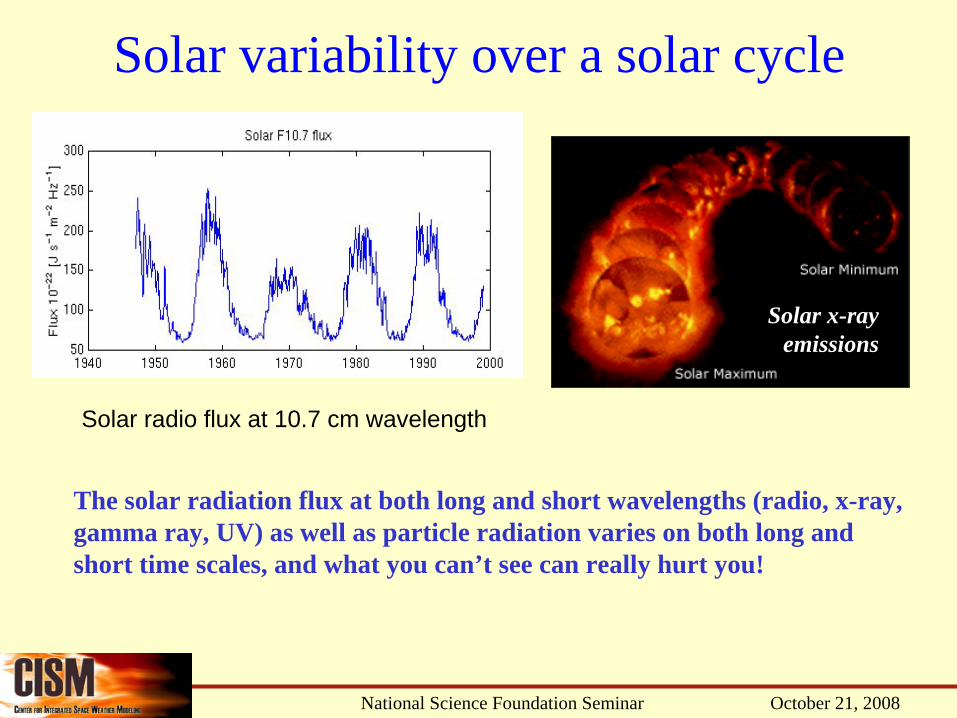
Solar variability over a solar cycle

The solar radiation flux at both long and short wavelengths (radio, x-ray, gamma ray, UV) as well as particle radiation varies on both long and short time scales, and what you can’t see can really hurt you!

Solar x-rayemissions

Solar radio flux at 10.7 cm wavelength


The Sun imaged in extreme ultraviolet (EUV), 195 Å, by the SOHO spacecraft showing the Sun’s outer atmosphere, the corona, at a temperature of1.5 million K

Short time scale EUV variations


Overview of Solar X-rays and Solar Protons: December 2006 storms

X-rays(flares)

EnergeticProtons(100’s keV

– 100’s MeV)

X flareM flareC flare

From: Uccellini et al, NOAA/NCEP Memo on NOAA Region 10930


Hinode Solar Optical Telescope: high-resolution observations of the Dec 13, 2006 flare with flare

ribbons above the sunspot


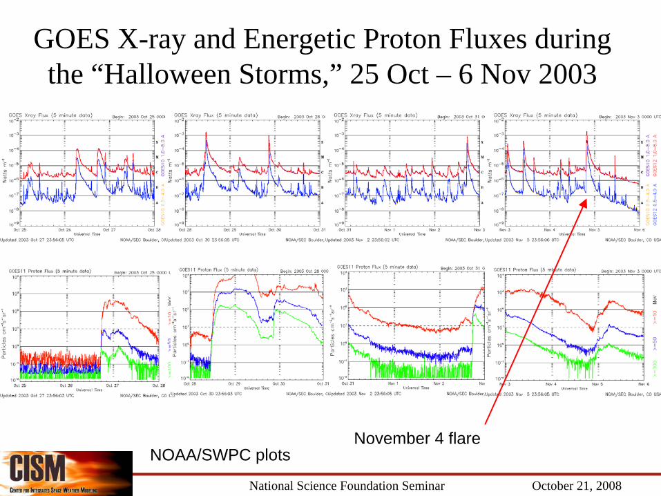
GOES X-ray and Energetic Proton Fluxes during the “Halloween Storms,” 25 Oct – 6 Nov 2003

November 4 flareNOAA/SWPC plots


Soft X-ray image of November 4 flare on the solar limb


Simple model of a solar flare involving magnetic reconnection in the corona

Cusped magnetic loopsLoops move downward cooling as they fall. Loops are visible at a given wavelength only as they pass through a narrow temperature range Flare ribbons in chromosphere

Chromosphere is heated by gas flowing down from reconnection siteflows


The Sun’s outer corona continually streams away from the sun forming the solar wind, a supersonic outflow of a very tenuous plasma with an entrained magnetic field.

The Solar Wind and Coronal

Mass Ejections


SOHO coronagraph images of the 30 July 2005 Coronal Mass Ejection (CME)

6:50 UT 7:53 UT


Simple model of a CME: a solar prominence released by magnetic reconnection

Reconnection of sheared loops creates a magnetic flux rope


The challenge of operational predictions

(from NOAA/SWPC)


(From AFRL)


Mission:• Introduce Sun-to-Earth Community Models into

space physics• Introduce physics-based numerical models into

space weather operational prediction and forecasting

• Imbue the notion that sun-earth science is a single unified discipline

NSF Science and Technology Center (STC): Funded September 2002

Vision: To understand our dynamic sun-earth system and how it affects life and society.

Center for Integrated Space Weather Modeling


Center for Integrated Space Weather ModelingThe CISM Mission is enabled by its unifying GOAL:

To develop and validate coupled physics-based numerical simulation models that describe the space environment from the Sun to the Earth.

USES:• Scientific tools for increased understanding of the

complex space environment.• Specification and forecast tools for space weather

prediction.• Education tools for teaching about the space

environment.MANDATE: in the National Space Weather Program plan


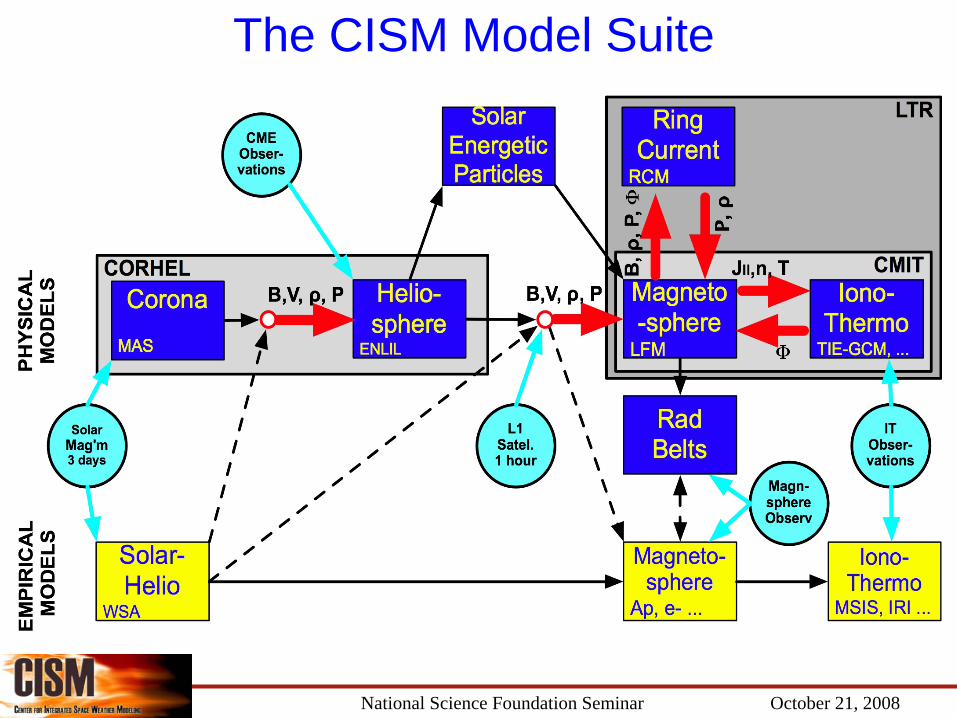
The CISM Model Suite


Core CISM Solar & Heliospheric Models

MAS (coronaand CMEs) ENLIL (solar wind

and cone model forICMEs)


Using observed solar magnetograms as input, a magnetohydrodynamic (MHD) simulation provides the 3-D structure of the coronal magnetic field

A solar magnetogram – the surface magnetic field derived spectroscopically

http://sohowww.nascom.nasa.gov/data/realtime/mdi_mag/


MAS predictions for August 1 Solar Eclipse

Eclipse path

Predicted coronal image at totalityCalculated coronal magnetic field

(published by SAIC a week earlier)


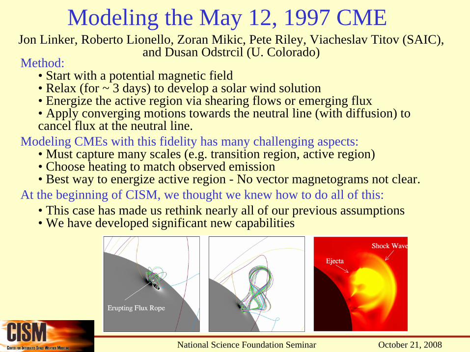
Modeling the May 12, 1997 CME

Method: • Start with a potential magnetic field • Relax (for ~ 3 days) to develop a solar wind solution • Energize the active region via shearing flows or emerging flux • Apply converging motions towards the neutral line (with diffusion) to cancel flux at the neutral line.

Modeling CMEs with this fidelity has many challenging aspects: • Must capture many scales (e.g. transition region, active region) • Choose heating to match observed emission • Best way to energize active region - No vector magnetograms not clear.

At the beginning of CISM, we thought we knew how to do all of this:• This case has made us rethink nearly all of our previous assumptions • We have developed significant new capabilities

Jon Linker, Roberto Lionello, Zoran Mikic, Pete Riley, Viacheslav Titov (SAIC), and Dusan Odstrcil (U. Colorado)


May 12, 1997 CME: Comparison of the Simulated Pre-event Corona with Observations

-2 -1.2 -.4 .4 1.2 2 2.8 0 1 2 3 4Log10 (DN/s)

EIT 171ÅEIT 195Å

EIT 284Å SXT (composite)

-1 -.1 .8 1.7 2.6 3.5

EIT 195Å

EIT 195Å EIT 284Å SXT (composite)


Flux preserving vortical flow introduced to build energy

Δsmax = 0

Δsmax = 0.056 rad

Δsmax = 0.013 rad

Δsmax = 0.11 rad

Energization of the Magnetic Field

Propagation of the Simulated CME into the Corona

6.8 hours after Flux Cancellation begins 8.8 hours7.8 hours

Polarization Brightness

Magnetic Field Lines


Evolution of magnetic field during May 12 eruption


• CME flux rope starts out connected to active region.• As CME propagates, it reconnects with nearby open field andloses connection with the active region


Structure expands to outer edge of MAS solution domain at 20 RSun


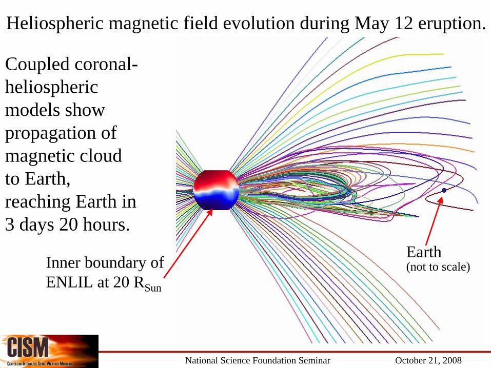
Coupled coronal- heliospheric models show propagation of magnetic cloud to Earth, reaching Earth in 3 days 20 hours.

Heliospheric magnetic field evolution during May 12 eruption.

Inner boundary of ENLIL at 20 RSun

Earth(not to scale)


Fast stream follows the ICME

May 12, 1997 Coronal Mass Ejection (CME) simulated with the Cone Model in the ENLIL Solar Wind MHD Model


Geospace coupling is currently single ENLIL grid point-based

ICME

SHOCK

L1-EARTH


Insert animation CmitPC.avi here

Size to fill slide

available from:

download.hao.ucar.edu/pub/stans/gold/goldpc

(if it doesn’t work, then delete this slide)

GeospaceMagnetosphere, Ionosphere and Thermosphere


Entry of solar wind plasma into the magnetosphere – using Multi-Fluid LFM Peter Damiano, John Lyon, Bill Lotko (Dartmouth Coll.)

• Plasma is split into two identical proton fluids (Blue and Yellow)– Initially 99.99% Blue fluid and 0.01% Yellow– At start of inflow, solar wind is flipped the other way (0.01%

Blue, 99.99% Yellow)– Watch how the Yellow fluid enters the magnetosphere.

• Standard solar wind conditions– 400 kms– N = 5/cc– IMF, Bz = -5 nT


Equatorial planeNoon-midnight meridian plane


Effect of outflowing polar O+ ion fluid on tail dynamics

Without O+ outflow With O+ outflow


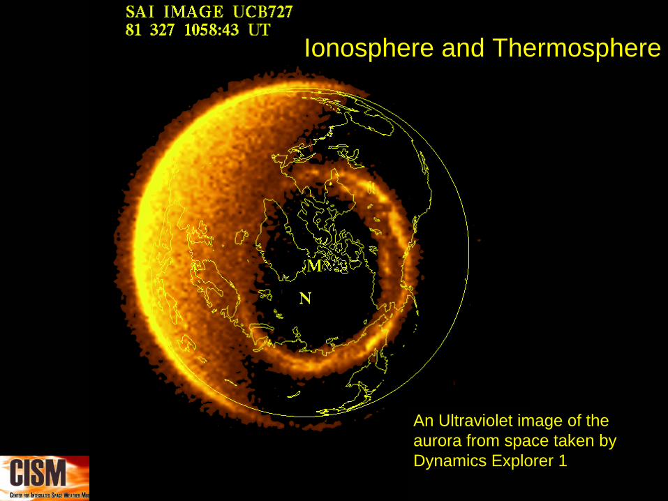
An Ultraviolet image of the aurora from space taken by Dynamics Explorer 1

Ionosphere and Thermosphere


The North Amerian AnomalyΔ

TEC from TIE-GCM Δ

TEC from CMIT Δ

TEC from GPS


Processes Driving Changes in Electron Density


Comparison between CMIT and Millstone Hill Incoherent Scatter Radar


What are we proud of? Crossing the Valley of Death: Moving research models into operational space weather forecasting through our partnership with the NOAA Space Weather Prediction Center (SWPC)

NRC Report: From Research to Operations in Weather Satellites and Numerical Weather Prediction: Crossing the Valley of Death

The Operations Room, NOAA/NWS/SWPC, Boulder Colorado


WSA-ENLIL: 2008 January 6-15 – Flow Velocity


WSA-ENLIL-Cone Model of CME’s: 2007 January 24-25


Geomagnetic disturbances from CMIT

Transition is in initial stages.


What are we proud of? Our graduate student community.Building a strong community of graduate student across institutions & disciplines– Annual graduate student retreats – Graduate students are integral team members– Students have been involved in many cross-institution papers – Graduate student community has become self organized

CISM Graduate students on retreat.


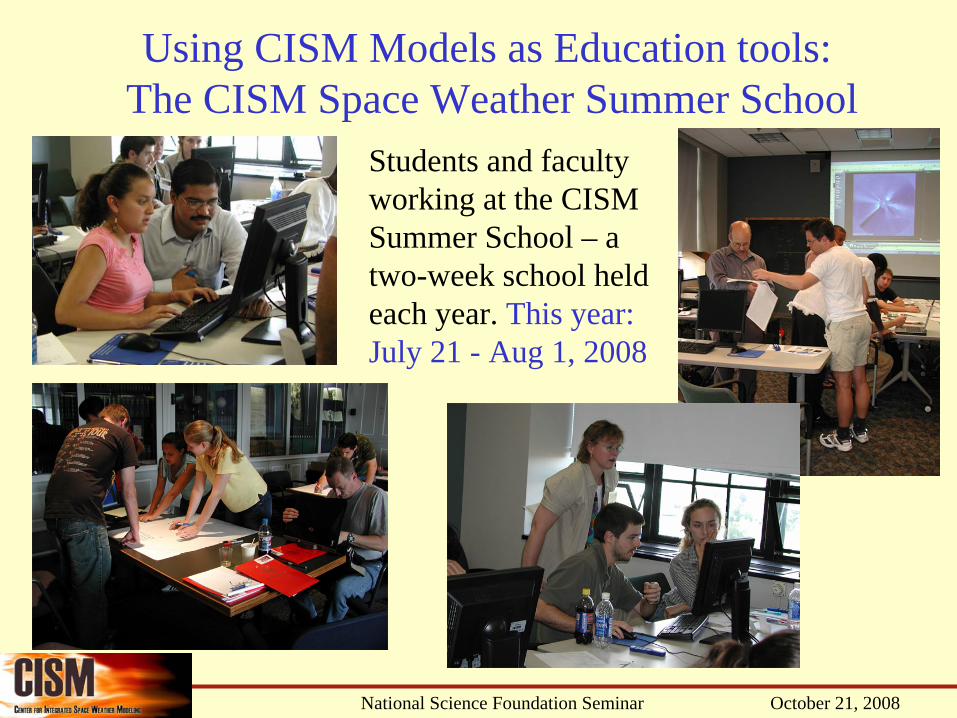
Using CISM Models as Education tools: The CISM Space Weather Summer School

Students and faculty working at the CISM Summer School – a two-week school held each year. This year:July 21 - Aug 1, 2008


What We’ve Learned

• Center structure has allowed CISM a coherent approach to a complex problem.

• Plans need to be flexible and be changed as we learn more.

• Coupled models have led to understanding of coupled processes.

• Crossing the valley of death is difficult, but possible with good collaboration.

storms in space: understanding and predicting space weather · storms in space: understanding and...

Documents