precursory scale increase and long-term seismogenesis in california and northern mexico

ANNALS OF GEOPHYSICS, VOL. 45, N. 3/4, June/August 2002

479

Precursory scale increase and long-termseismogenesis in California

and Northern Mexico

Frank Evison (1) and David Rhoades (2)(1) Institute of Geophysics, Victoria University of Wellington, New Zealand(2) Institute of Geological and Nuclear Sciences, Lower Hutt, New Zealand

AbstractA sudden increase in the scale of seismicity has occurred as a long-term precursor to twelve major earthquakes inCalifornia and Northern Mexico. These include all earthquakes along the San Andreas system during 1960-2000with magnitude M 6.4. The full list is as follows: Colorado Delta, 1966, M 6.3; Borrego Mt., 1968, M 6.5; SanFernando, 1971, M 6.6; Brawley, 1979, M 6.4; Mexicali, 1980, M 6.1; Coalinga, 1983, M 6.7; Superstition Hills,1987, M 6.6; Loma Prieta, 1989, M 7.0; Joshua Tree, 1992, M 6.1; Landers, 1992, M 7.3; Northridge, 1994, M6.6; Hector Mine, 1999, M 7.1. Such a Precursory Scale Increase ( ) was inferred from the modelling of long-term seismogenesis as a three-stage faulting process against a background of self-organised criticality. The location,onset-time and level of are predictive of the location, time and magnitude of the future earthquake. Precursoryswarms, which occur widely in subduction regions, are a special form of ; the more general form is here shownto occur frequently in a region of continental transform. Other seismicity precursors, including quiescence andforeshocks, contribute to or modulate the increased seismicity that characterises . The area occupied by issmall compared with those occupied by the seismicity precursors known as AMR, M 8 and LURR. Further workis needed to formulate as a testable hypothesis, and to carry out the appropriate forecasting tests.

1. Introduction

Anomalies of seismicity are intuitively themost plausible of all proposed earthquakeprecursors. The universal power-law relatingearthquake magnitude and frequency shows thateach earthquake of magnitude M has associatedwith it, in a statistical sense, about three hundredearthquakes of magnitude M-2.5 or greater. For

a shallow earthquake, aftershocks typicallyprovide about one-tenth of these associatedsmaller earthquakes. Immediate preshocks,commonly known as foreshocks, seldom providemore than a few, and often none at all. What aboutpreshocks occurring over longer time periods,and perhaps larger areas? The M 8 model(Kossobokov et al., 1999) and the AcceleratingMoment Release (AMR) model (Varnes, 1989;Bowman et al., 1998) are both concerned withpreshocks over moderately long time periods andover large areas. Shorter time periods and largeareas are specified in the Load/Unload ResponseRatio (LURR) model (Yin et al., 2000). In thepresent study, the time period is the longest sofar suggested for a precursory phenomenon (apartfrom regular recurrence models), while the areais comparatively small.

Mailing address: Prof. Frank F. Evison, Institute ofGeophysics, Victoria University of Wellington, P.O. Box 600,Wellington, New Zealand; e-mail: [email protected]

Key words precursory seismicity – seismogenesis –California – Mexico

480

Frank Evison and David Rhoades

Seismicity precursors are also the easiest tostudy, because of the very large databasecontained in observatory catalogues. Manyworkers consider that it simplifies matters todecluster the catalogue, i.e. to remove aftershocks(Reasenberg, 1985), and perhaps other con-centrations of small earthquakes as well. In thepresent study the whole catalogue is used, apartfrom applying a magnitude threshold in theinterest of homogeneity. Earthquake concen-trations, including aftershocks, are found to behighly relevant to the understanding of seis-mogenesis.

Second only to aftershock sequences, theeasiest concentration of earthquakes to recognisein many catalogues is the swarm. Swarms arecommon in the shallow seismicity of subductionregions: systematic studies in New Zealand,Japan and Greece show that swarms make a largecontribution to long-term preshock activity insubduction regions, where swarms are predictiveof mainshocks (Evison and Rhoades, 2000). Thisphenomenon is explained by modelling seismo-genesis as a three-stage faulting process occur-ring against a background of self-organisedcriticality (Evison and Rhoades, 1998, 2001).An inference from the model, however, is thatpreshocks need not occur as swarms. This hasbeen confirmed in a region of continental col-lision (Evison and Rhoades, 1999a): the pre-cursor is a long-term set of preshocks, irre-spective of how they are distributed in time. Thepresent paper extends the study to a region ofcontinental transform, and better defines theprecursor as a sudden increase in the scale oflong-term minor seismicity in the neighbourhoodof the future mainshock. The aim is to show thatthe scale increase is a seismogenic phenomenon,preparatory to formulating an hypothesis that canbe tested by long-range forecasting.

2. The -phenomenon

The precursory scale increase, here called the-phenomenon, is a seismicity pattern in space,

magnitude and time. The essential features of thephenomenon are shown schematically in thethree diagrams in fig. 1a-c. First, the area oc-cupied by the phenomenon indicates the location

and space-scale of the seismogenic process(fig. 1a). This is found by adjusting the position,size and shape of a rectangular area containingthe main-shock and aftershocks, so as to obtainthe highest seismicity rate in the precursory pe-riod relative to the rate in the prior period (seefig. 1c). Such a procedure could be refined byformal optimisation, which could readily allowfor areas to be elliptical, with any orientation,rather than the present N-S, E-W rectangles. Forthe 12 examples presented below, the medianmain-shock magnitude is M6.6, and the medianarea is 4500 km2. All earthquakes that occur inthe rectangle (and have magnitudes at or abovethe threshold) are included in the analysis.

Secondly, the magnitude level MP of theprecursory seismicity (fig. 1b) determines themagnitude-and-time scale of the seismogenicprocess. A robust measure of magnitude level,adopted here as in previous studies of the swarmprecursor, is the average of the three largestmagnitudes in the relevant time-period. Sincemuch of the precursory seismicity tends to occurearly in the precursory period, a good estimateof this magnitude level, which is a crucialseismogenic parameter, is usually available at anearly stage.

Thirdly, the jump in seismicity that marks theonset of seismogenesis is indicated by the suddenchange of slope in fig. 1c. This graph is a cumu-lative magnitude anomaly (cumag), C(t), whichis a type of cusum (Page, 1954) designed todisplay the average rate of seismicity betweenany two points in time. C(t) is defined by

(2.1)

(2.2)

where Mi is the magnitude and ti the time of theith earthquake, Mc is the threshold magnitude,and k is the average rate of magnitude accu-mulation between the starting time ts and thefinishing time tf . Accordingly, each earthquake

C t M M k t tts ti t i c s( ) = +( ) ( )0 1.

k M M t tts ti t f i c f s= +( ) ( )0 1. /

481

Precursory scale increase and long-term seismogenesis in California and Northern Mexico

micity rate expressed in units of magnitudeper year (MU/yr) for the relevant area. (Forexample, if the chosen threshold magnitude (Mc)is 4.0, and in a particular interval of a year thereoccurs a single earthquake, with magnitude 4.9,the seismicity rate for that time interval is 1.0MU/yr). A major upward jump in rate producesa sharp minimum in the C(t) graph; the low pointis taken as the onset of the -anomaly, and thedate of the low point marks the start of theprecursor time TP . The precursory rate is thengiven by the gradient of the straight line joiningthe low point to the zero point immediatelybefore the mainshock, while the prior rate isobtained by joining the initial zero point to thelow point.

throughout the sequence is represented by anupward jump equal to the amount by which themagnitude exceeds the baseline value, which is0.1 below the threshold magnitude. The down-ward slope between successive earthquakes isequal and opposite to the sum of all the upwardjumps, divided by the total time; thus, a givenplot begins and ends at the value zero. Unlikemost cusum graphs, the cumag abscissa is a linearscale of time.

From eqs. (2.1) and (2.2) it follows that thegradient of the line between any two points onthe C(t) curve is a measure of the average rate ofearthquake activity during the correspondingtime period. Gradients are translated into seis-micity rates by means of a protractor, with seis-

.

Fig. 1a-c. -phenomenon: schematic. a) Typical epicentral area of precursory seismicity, mainshock and after-shocks. b) Prior magnitude level and jump to precursory level MP. Magnitude level is derived from the data: it isthe average of the three largest magnitudes in the relevant period of time. Mm is the mainshock magnitude. c) Priorand precursory seismicity rates, showing sudden change at start of precursor time TP. Seismicity rate is derivedfrom the data by means of the cumag (see eqs. (2.1) and (2.2)); it is averaged over the relevant period of time. Aprotractor is included to indicate the rate corresponding to any given slope; rate is given in units of magnitudeabove base-level, per year (MU/yr).

482


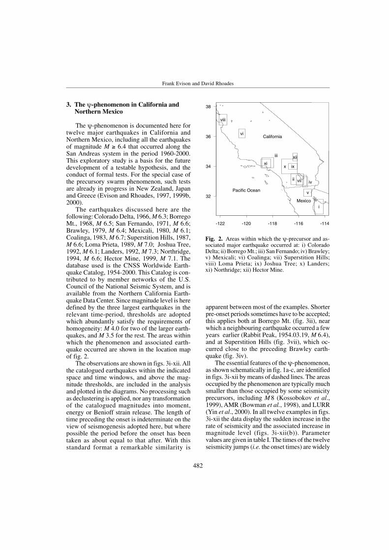
3. The -phenomenon in California andNorthern Mexico

The -phenomenon is documented here fortwelve major earthquakes in California andNorthern Mexico, including all the earthquakesof magnitude M 6.4 that occurred along theSan Andreas system in the period 1960-2000.This exploratory study is a basis for the futuredevelopment of a testable hypothesis, and theconduct of formal tests. For the special case ofthe precursory swarm phenomenon, such testsare already in progress in New Zealand, Japanand Greece (Evison and Rhoades, 1997, 1999b,2000).

The earthquakes discussed here are thefollowing: Colorado Delta, 1966, M 6.3; BorregoMt., 1968, M 6.5; San Fernando, 1971, M 6.6;Brawley, 1979, M 6.4; Mexicali, 1980, M 6.1;Coalinga, 1983, M 6.7; Superstition Hills, 1987,M 6.6; Loma Prieta, 1989, M 7.0; Joshua Tree,1992, M 6.1; Landers, 1992, M 7.3; Northridge,1994, M 6.6; Hector Mine, 1999, M 7.1. Thedatabase used is the CNSS Worldwide Earth-quake Catalog, 1954-2000. This Catalog is con-tributed to by member networks of the U.S.Council of the National Seismic System, and isavailable from the Northern California Earth-quake Data Center. Since magnitude level is heredefined by the three largest earthquakes in therelevant time-period, thresholds are adoptedwhich abundantly satisfy the requirements ofhomogeneity: M 4.0 for two of the larger earth-quakes, and M 3.5 for the rest. The areas withinwhich the phenomenon and associated earth-quake occurred are shown in the location mapof fig. 2.

The observations are shown in figs. 3i-xii. Allthe catalogued earthquakes within the indicatedspace and time windows, and above the mag-nitude thresholds, are included in the analysisand plotted in the diagrams. No processing suchas declustering is applied, nor any transformationof the catalogued magnitudes into moment,energy or Benioff strain release. The length oftime preceding the onset is indeterminate on theview of seismogenesis adopted here, but wherepossible the period before the onset has beentaken as about equal to that after. With thisstandard format a remarkable similarity is

apparent between most of the examples. Shorterpre-onset periods sometimes have to be accepted;this applies both at Borrego Mt. (fig. 3ii), nearwhich a neighbouring earthquake occurred a fewyears earlier (Rabbit Peak, 1954.03.19, M 6.4),and at Superstition Hills (fig. 3vii), which oc-curred close to the preceding Brawley earth-quake (fig. 3iv).

The essential features of the -phenomenon,as shown schematically in fig. 1a-c, are identifiedin figs. 3i-xii by means of dashed lines. The areasoccupied by the phenomenon are typically muchsmaller than those occupied by some seismicityprecursors, including M 8 (Kossobokov et al.,1999), AMR (Bowman et al., 1998), and LURR(Yin et al., 2000). In all twelve examples in figs.3i-xii the data display the sudden increase in therate of seismicity and the associated increase inmagnitude level (figs. 3i-xii(b)). Parametervalues are given in table I. The times of the twelveseismicity jumps (i.e. the onset times) are widely

Fig. 2. Areas within which the -precursor and as-sociated major earthquake occurred at: i) ColoradoDelta; ii) Borrego Mt.; iii) San Fernando; iv) Brawley;v) Mexicali; vi) Coalinga; vii) Superstition Hills;viii) Loma Prieta; ix) Joshua Tree; x) Landers;xi) Northridge; xii) Hector Mine.

483


Fig. 3i,ii. -phenomenon: data and interpretation for major earthquakes at (i) Colorado Delta and (ii) BorregoMt. Interpretation is explained in fig.1a-c. a) Epicentres. b) Magnitudes versus time, also showing (dashed lines)the derived prior and precursory magnitude levels. c) Cumag (eqs. (2.1), (2.2)), also showing (dashed lines) thederived prior and precursory seismicity rates. (The cumag scale on the right-hand side refers to the mainshock-aftershock period).

484


Fig. 3iii,iv. -phenomenon: data and interpretation for major earthquakes at (iii) San Fernando and (iv) Brawley.For explanation see caption fig. 3i,ii.

485


Fig. 3v,vi. -phenomenon: data and interpretation for major earthquakes at (v) Mexicali and (vi) Coalinga. Forexplanation see caption fig. 3i,ii.

486


Fig. 3vii,viii. -phenomenon: data and interpretation for major earthquakes at (vii) Superstition Hills and (viii)Loma Prieta. For explanation see caption fig. 3i,ii.

487


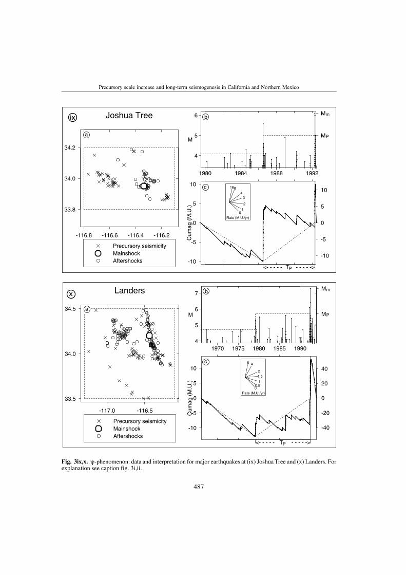
Fig. 3ix,x. -phenomenon: data and interpretation for major earthquakes at (ix) Joshua Tree and (x) Landers. Forexplanation see caption fig. 3i,ii.

488


Fig. 3xi,xii. -phenomenon: data and interpretation for major earthquakes at (xi) Northridge and (xii) HectorMine. For explanation see caption fig. 3i,ii.

489


NB: M is the prior magnitude level; MP is the precursory magnitude level; TP is the time in days between the onsetof seismogenesis and the mainshock; scale increase M is MP minus M ; scale increase rate is precursory rate/priorrate.

Table I. Precursory scale increase ( ) data.

Locality Prior Onset Precursory Scale Mainshock increase

M Rate Date MP Rate TP(d) M Rate Date Mm

Colorado D. 4.2 0.82 1964.01.17 5.1 11.57 933 0.9 14.04 1966.08.07 6.3Borrego Mt. 4.1 1.38 1957.01.24 5.1 5.42 4093 1.0 3.92 1968.04.09 6.5S. Fernando 3.5 0.03 1964.02.08 4.1 0.56 2558 0.6 19.79 1971.02.09 6.6Brawley 3.6 0.16 1974.12.06 4.8 6.55 1774 1.2 40.37 1979.10.15 6.4Mexicali 4.3 1.12 1976.01.03 5.0 5.89 1619 0.7 5.27 1980.06.09 6.1Coalinga 3.8 0.23 1975.01.06 5.1 2.07 3038 1.3 8.83 1983.05.02 6.7Super. Hills 3.6 0.44 1981.04.25 5.6 4.22 2404 2.0 9.70 1987.11.24 6.6Loma Prieta 4.7 0.30 1979.05.08 5.9 1.89 3816 1.2 6.34 1989.10.18 7.0Joshua Tree 4.1 0.87 1986.07.08 5.0 4.00 2116 0.9 4.61 1992.04.23 6.1Landers 4.7 0.42 1979.03.15 5.7 2.37 4854 1.0 5.59 1992.06.28 7.3Northridge 3.5 0.07 1988.11.21 4.8 1.71 1883 1.3 23.00 1994.01.17 6.6Hector Mine 3.5 0.05 1992.06.28 5.0 1.72 2667 1.5 32.29 1999.10.16 7.1

scattered between 1957 and 1992. This makes itunlikely that the -phenomenon in California andNorthern Mexico could be an artificial effectproduced by improvements in the seismographnetwork.

The scale increase in magnitude ranges from0.6 to 2.0 magnitude units, with a median of 1.1.The scale increase in rate ranges from 3.92 to40.37, with a median of 9.27. These medianvalues correspond rather closely; for twoGutenberg-Richter sets with b-values of unity, ajump of 1.0 magnitude units would correspondto a scale increase of 10. The wide range of valuesfor each of the measures of scale increase is tobe expected, on the present view of seismo-genesis, since the level of seismicity in the priorperiod, like the length of that period, is inde-terminate, and has no effect on the seismogenicprocess. (It should be noted that the rates in tableI are not to be compared from one example toanother, since they depend on the size of therelevant area, as well as on the adopted thresholdmagnitude).

In many of the examples the mainshockepicentre is near the centre of the rectangle, but

this is not always to be expected, since the hypo-centre may occur at any point on the fracture. AtColorado Delta (fig. 3i) and at Brawley (fig. 3iv),the mainshock epicentre is near the edge of therectangle, while aftershocks are located amongthe precursory seismicity.

Once the occurrence of a jump in the rate ofseismicity indicates that seismogenesis hasbegun, it is the time of the jump, and the valueof the new magnitude level, that allow the para-meters of the major earthquake to be estimated,as will be explained below. The precursory rategiven in table I is that for the whole precursoryperiod. The rate up to any earlier point canequally be obtained, from the slope of the cumagbetween the time of the jump and that of the pointin question. Thus it is easy to see to what extentthe occurrence of a -anomaly would becomeapparent at an early stage, for example if theseismicity were being monitored in real time. Thecumags in figs. 3i-xii show that rates that wouldbe observed early in the precursory period areusually higher than the final value; i.e. lines fromthe low point to intermediate points along theprecursory data-plot are usually steeper than the

490


dashed line. At Superstition Hills (fig. 3vii), thisis so for about the first half of the precursoryperiod, but the -anomaly could hardly havebeen recognised, because of the short time thatelapsed between the nearby Brawley earthquake(fig. 3iv) and the change of scale at SuperstitionHills. In addition, many of the precursory earth-quakes at Superstition Hills occurred as immediateforeshocks, thus adding to the unusual appear-ance of the cumag graph. (The dashed line in fig.3vii(b) (lower), as in the other cumag graphs infigs. 3i-xii, indicates the average seismicity ratefrom the time of the scale increase to immediatelybefore the mainshock). Despite these com-plications, the parameter values given in table Ifor Superstition Hills are compatible with thosefor the other examples.

The precursory earthquakes, like the after-shocks, contribute directly to the set of minor earth-quakes associated with the major earthquake.The two contributions appear to be roughlycomparable, since the magnitude levels are aboutthe same (Evison and Rhoades, 1998). Together,therefore, they contribute roughly one-fifth of theminor earthquakes that are statistically associatedwith the mainshock through the Gutenberg-Richter relation. The remaining four-fifths evi-dently occur outside the seismogenic location-time space; in this larger space the mainshockwould not stand out as anomalously large.

The following correlations support the viewthat the -anomaly is a seismogenic pheno-menon, and suggest how it might be applied tolong-range earthquake forecasting.

4. Predictive correlations

The -phenomenon is related to the majorearthquake in location, magnitude and time. Theepicentres of the precursory seismicity arelocated close to those of the mainshock andaftershocks, as shown in figs. 3i-xii(a). Secondly,the relation between mainshock magnitude (Mm)and precursor magnitude (MP) agrees closely withthe regression that has previously been calculatedfor the swarm phenomenon (fig. 4a). Thirdly,agreement is also evident with the relationbetween precursor time (TP) and precursor mag-nitude (fig. 4b).

These agreements are to be expected, sinceprecursory swarms are a special form of the -phenomenon. The set of precursory earthquakesmay occur in a variety of ways. In the shallowsubduction regions of Greece, Japan and NewZealand they occur in the highly organized andrecognizable form of swarms. In California andNorthern Mexico, on the other hand, many dif-ferent types of distribution occur, as can be seenin figs. 3i-xii. The agreement with regard to

Fig. 4a,b. Predictive regressions (after Evison andRhoades, 2000) obtained from systematic studies inGreece, Japan and New Zealand, with California andNorthern Mexico data superimposed. a) Mainshockmagnitude versus precursor magnitude. b) Precursortime versus precursor magnitude. NB: Precursormagnitude and precursor time refer to the special caseof the swarm precursor for the Greece, Japan and NewZealand data, and to the more general -precursor forthe California and Northern Mexico data.

491


precursor time depends in part on the tendencyof swarms to occur early in the precursory period,i.e. at or soon after the onset of seismogenesis.

Taking the swarm and results together, therelations between precursor and mainshock asregards magnitude and time are now supported,as fig. 4a,b shows, by 40 examples of majorearthquakes in New Zealand, Japan, Greece,California and Northern Mexico. The presentstudy has yet to be extended to include a searchfor instances of the -phenomenon occurringunrelated to a mainshock event, or vice versa.Nevertheless, the new results help to sharpen thedefinition of the -phenomenon, and theyaugment the empirical basis both for testing thepredictive capability of the phenomenon and formodelling seismogenesis.

5. Three-stage faulting model

A minor variation on the accepted process offaulting - crack formation, shear fracture, healing- is sufficient to account for the above corre-lations. This variation is to regard crack formationas a stage that is separable in time from theconsequent shear fracture. A major fault such asthe San Andreas is the result of many suchfaulting processes through geologic time. As acorollary of the separation of crack formationfrom shear fracture, it is postulated that a majorcrack generates a set of minor cracks, in the sameway that, in the mainshock/aftershock pheno-menon, a major fracture generates a set of minorfractures.

Modelling the faulting process in threeseparable stages was first proposed to accountfor the precursory swarm phenomenon (Evisonand Rhoades, 1998). An inference from themodel, however, was that precursory earthquakesneed not occur as swarms. This extended thescope of the long-term seismicity precursor toregions where swarms do not usually occur,i.e. to other than subduction regions. In thecontinental collision region of New Zealand,swarms are replaced by more dispersed groupsof precursory earthquakes, which have beencalled quasi-swarms, or quarms (Evison andRhoades, 1999a). The present study is the firstin which a sudden increase in the scale of seis-

micity is taken as the precursor; this is the mostgeneral form suggested by the model.

Under the three-stage faulting model, theformation of a major crack starts the processwhich eventually culminates in a major shearfracture (and the resultant major earthquake). Themajor crack at once generates a set of minoraftercracks, which fracture over time, and it isthese minor fractures that produce the precursoryseismicity. Healing of the set of minor fracturesis a necessary condition for the fracture of themajor crack, which generates the mainshock andaftershocks. Finally, healing of these fracturesrestores the medium to the condition it was inbefore the particular process started.

Three-stage faulting accounts, then, for thefollowing features of the -phenomenon. Thejump increase in seismicity marks the onset offracturing of the set of aftercracks generated bythe major crack. It has been observed that theset of precursory earthquakes has a similarmagnitude level to the aftershocks (Evison andRhoades, 1998); this follows, in the model, fromthe major crack and fracture being necessarilyof the same size. (In the 12 examples presentedhere the ratio of aftershock to precursormagnitude level ranges from 0.84 to 1.37, witha median of 0.99). The long duration of theseismogenic process is explained by the need,according to Mogi’s (1963) criteria, for the stressfield across a fault to become uniform beforefracture can occur; uniformity across the majorcrack is attained by the healing of the set ofaftercracks, after they have fractured andgenerated the precursory earthquakes. Finally, theessential independence of major earthquakesfrom one another is explained by the healingwhich follows the mainshock and aftershocks.Inter-earthquake triggering, while not excluded,occurs as a second-order effect. The failure ofexperiments based on the regular-recurrencehypothesis, such as the experiment at Parkfield,California (Roeloffs and Langbein, 1994), isexplained.

The seismogenic process as modelled bythree-stage faulting is further elucidated by theproposal that it takes place against a backgroundof self-organised criticality (Evison and Rhoades,2001). Self-Organised Criticality (SOC) systemsdisplay an extreme sensitivity to initial con-

492


ditions. Thus under the model it is acknowledgedthat the sudden increase in seismicity may be theearliest recognisable signal of a future majorearthquake, just as in meteorology, where SOCis the widely accepted background condition, atropical depression is the earliest signal of a futuretropical cyclone. The scaling principle, which isalso basic to SOC, is exemplified in the modelby the role of the major crack in determining thescale of the entire seismogenic process, withregard to space, magnitude and time. Thus theterm «major» is purely relative: the major crackcan be of any absolute size. Again, the SOCprinciple of hierarchy is exemplified in theoccurrence of smaller seismogenic processesembedded in larger ones, as with the Joshua Treeprocess (fig. 3ix), which was entirely embedded inthe precursor to the Landers earthquake (fig. 3x).

More generally, the context of a given majorearthquake can be understood in two distinctways, depending on scale. On the larger scale,as already mentioned above, the earthquakebelongs to a Gutenberg-Richter set, and occursin a context of self-similarity. On the smallerscale, the earthquake is anomalous: as a main-shock, it is too large to belong to the Gutenberg-Richter set of its preshocks and aftershocks.This is the scale of the predictive correlationsthat have been presented above.

Under self-organized criticality, one canvisualise that any of a large number of smallearthquakes has the potential to avalanche, thusnucleating a large earthquake. This has beeninterpreted to mean that individual earthquakesare intrinsically unpredictable. The present modelreconciles long-range forecasting with self-organized criticality by accommodating theavalanche-nucleation concept at the crack-formation stage of seismogenesis. There is noreason to regard the initial cracking as predictable,but once it has occurred the remaining stages,including the major earthquake, are determined.

This is somewhat analogous to the nucleationand development of a tropical cyclone.

6. Associated precursors

Several types of precursor occur as fluc-tuations which modulate the average seismicity

during the precursory period. Large swarms markthe onset of seismogenesis at Colorado Delta(fig. 3i) and Borrego Mt. (fig. 3ii). Foreshocksoccur at the end of the precursory period, occasion-ally in large numbers, as at Superstition Hills(fig. 3vii) and at Landers (fig. 3x). In contrast,quiescence frequently occurs, as at Northridge(fig. 3xi) and Hector Mine (fig. 3xii), in both ofwhich an interval occupying about 40% of theprecursory period was devoid of earthquakes.The well-known accelerating moment releaseprecursor will be discussed in detail below.

A seismicity parameter frequently studiedin the context of precursory phenomena is theb-value in the Gutenberg-Richter equationlog10N(M) = a bM. A related parameter isthe mean magnitude of a Gutenberg-Richter set(Aki, 1965). The Loma Prieta and Northridgeearthquakes have been studied by Smith (1998)in terms of precursory changes in meanmagnitude. The areas considered are similar tothose in fig. 3viii and fig. 3xi. Using two differenttypes of cusum graph, Smith found an anomalybefore the Loma Prieta earthquake, beginning atabout the same time as the -anomaly report-ed above. This may be a coincidence, since -anomalies are closely related to the a-value inthe Gutenberg-Richter equation, and this isusually held to be independent of the b-value.

Precursors involving phenomena other thanseismicity may in some cases be compatible withthe present model. The crack-formation stage offaulting may produce anomalies in acousticemission (Scholz, 1990), and coda Q 1 (Jin andAki, 1989), due to a form of dilatancy. Here, thedilatancy will consist of a fractal set of cracks,rather than pores of more or less uniform size.Electromagnetic emissions, too, have been wide-ly reported in association with cracking (e.g., Guoet al., 1994). On the present model, all such crack-related anomalies are to be looked for early in theprecursory period.

Many of these precursors have been observed,but the reporting of examples remains largelyanecdotal. This is consistent with the three-stagefaulting model. The contributory precursorsinvolving seismicity are possible but not nec-essary under this model; further, most studies ofprecursors related to cracking have concentratedon time periods rather close to the mainshock time.

493


7. and AMR precursors

Contrasting interpretations of the seismicitypreceding major earthquakes are suggested bythe y and AMR (Accelerating Moment Release)patterns. A ready comparison can be madebetween these interpretations for California,since, of the earthquakes discussed above,Bowman et al. (1998) have presented detailedAMR interpretations of Borrego Mountain, SanFernando, Coalinga, Superstition Hills, LomaPrieta, Landers, and Northridge. The two studieshave different backgrounds. The AMR study wasa search for empirical support of a theoreticalmodel. The incentive for the study, on the otherhand, was an inference from the three-stagefaulting model, which was itself developed toexplain the precursory swarm phenomenon.

Widely differing areas around the earthquakesource are involved in the two interpretations.In AMR theory, an increasing correlation lengthin the regional stress field reaches a critical point,and this is when the earthquake occurs. Theprocess involves an area very much larger thanthe earthquake source area. In the case of , bycontrast, a three-stage faulting process is pos-tulated in the more immediate neighbourhood ofthe source area, although still involving faultsbesides that on which the major earthquakeoccurs. Figure 5 shows the areas of the AMRcircles in Bowman et al. (1998) and those of the

rectangles, for the same set of earthquakes.Also shown is Utsu’s (1961) relation betweenaftershock area and mainshock magnitude, andparallel lines are fitted to the AMR and sets ofdata. Overall, the areas are 10 times larger,and the AMR areas 140 times larger, than theaftershock areas. Further, the scatter is con-siderably less for the areas (variance 0.07) thanfor the AMR areas (variance 0.25).

One might think that the AMR phenomenonwould extend into the source region, but accor-ding to Jaumé and Sykes (1999) it occurs prima-rily outside. That no vestige of accelerating seis-micity occurs in most of the plots (figs. 3i-xii)is thus only to be expected. The exceptions areSuperstition Hills (fig. 3vii), Loma Prieta (fig. 3viii),and Landers (fig. 3x). These apparent oc-currences of accelerating seismicity were notidentified as AMR by Bowman et al. (1998), who

showed (their fig. 5) that for all the earthquakesthat they studied, except Loma Prieta, a linear ordecelerating moment release was indicated forareas of intermediate size.

Widely differing distributions of the precursoryseismicity with respect to time are also proposedby the two models. In AMR, the increase in seis-micity is initially emergent, and accelerates up tothe time of the earthquake, while in , the jump inseismicity occurs at the start of the precursoryperiod. This dominant feature of seems to beirrelevant to AMR, since in the plots given byBowman et al. (1998, fig. 6) for the BorregoMountain, San Fernando, Coalinga, SuperstitionHills and Northridge earthquakes, the starting datewas later than the jump in seismicity.

Little in common can thus be found betweenthe and AMR precursors. They may never-theless offer complementary information on thelocation, magnitude and time of future major

Mainshock magnitude

Are

a(1

000

sq.

km)

6.0 6.5 7.0 7.50.

11.

010

.010

0.0

AMRAftershocks (Utsu, 1961)

AMR

Ψ

Ψ

Fig. 5. and AMR precursory areas versus main-shock magnitudes for the earthquakes at BorregoMountain (1968, M 6.5); San Fernando (1971, M 6.6);Coalinga (1983, M 6.7); Superstition Hills (1987,M 6.6); Loma Prieta (1989, M 7.0); Landers (1992,M 7.3), and Northridge (1994, M 6.6). The Utsu (1961)relation between aftershock area and mainshockmagnitude is shown for comparison, and parallel linesare fitted to the AMR and data.

494


earthquakes. As regards location, the much largerareas involved in AMR are nevertheless centred,in the study by Bowman et al. (1998), on theearthquake epicentre. Robinson (2000) hasshown, however, in a study of three New Zealandearthquakes, that the AMR centre was best placedat a distance of 50-60 km from the earthquakeepicentre. As regards magnitude, AMR relatesthis to area, but as shown in fig. 5 above, there ismuch scatter in magnitude as a function of area.In the precursor, the mainshock epicentre canbe anywhere in the rectangular area, as discussedabove and exemplified in figs. 3i-xii(a), whilethe magnitude is given as a probability dis-tribution, with scatter as shown in fig. 4a.

The time of the major earthquake is indicatedin AMR by an exponentially increasing functionof the time to failure. This seems superior to theprobability distribution and scatter obtained forthe -precursor (fig. 4b). But according toRobinson (2000) the earthquake time estimatedby AMR is in practice only loosely constrained.

8. Conclusions

The -phenomenon is one of the simplestearthquake precursors so far identified. It ismanifested in the origin times, locations andmagnitudes routinely listed in earthquake cat-alogues. The predictive parameters that itsupplies consist of a rather closely defined area,a date, and a magnitude, and these give long-term estimates, in the form of probabilitydistributions, of the location, time and magnitudeof the major earthquake. As the longest-term ofall suggested precursors (unless one includes thehypothesised «seismic gap» as a precursor), itaccommodates a variety of shorter-term anom-alies. Precursory swarms, when they occur, area special case of the -precursor. Thus the aboveexamples from California and Northern Mexicocan be added to the 28 examples previouslypublished from Japan, Greece and New Zealand,making in all 40 large earthquakes that aresimilarly related to the -precursor. This consti-tutes a clear description of the -phenomenonas a long-term precursor, and part of the seis-mogenic process, in some of the main types ofseismotectonic environment. Formulation of a

testable hypothesis can now proceed, and bymeans of the appropriate methodology (Rhoadesand Evison 1979, 1993) the -precursor in Ca-lifornia, Northern Mexico and elsewhere can beevaluated for possible use in long-range earth-quake forecasting.

Acknowledgements

The authors thank E.G.C. Smith, W. D. Smithand J.J. Taber for critical readings of the manu-script, and Paolo Gasperini and an anonymousreviewer for valuable comments. The work hasbeen supported by the New Zealand Foundationfor Research, Science and Technology, underContract C05X0006. The first author acknow-ledges facilities provided under an HonoraryFellowship at Victoria University of Wellington.

REFERENCES

AKI, K. (1965): Maximum likelihood estimate of b in theformula log N = a bM and its confidence limits, Bull.Earthquake Res. Inst. Univ. Toyko, 43, 237-239.

BOWMAN, D.D., G. OUILLON, C.G. SAMMIS, A. SORNETTEand D. SORNETTE (1998): An observational test of thecritical earthquake concept, J. Geophys. Res., 103,24,359-24,372.

EVISON, F.F. and D.A. RHOADES (1997): The precursoryearthquake swarm in New Zealand: hypothesis tests II,N. Z. J. Geol. Geophys., 40, 537-547.

EVISON, F.F. and D.A. RHOADES (1998): Long-termseismogenic process for major earthquakes in subductionzones, Phys. Earth Planet. Inter., 108, 185-199.

EVISON, F.F. and D.A. RHOADES (1999a): The precursoryearthquake swarm and the inferred precursory quarm,N. Z. J. Geol. Geophys., 42, 229-236.

EVISON, F.F. and D.A. RHOADES (1999b): The precursoryearthquake swarm in Japan: hypothesis test, EarthPlanets Space, 51, 1267-1277.

EVISON, F.F. and D.A. RHOADES (2000): The precursoryearthquake swarm in Greece, Ann. Geofis., 43 (5), 991-1009.

EVISON, F.F. and D.A. RHOADES (2001): Model of long-termseismogenesis, Ann. Geofis., 44 (1), 81-93.

GUO, Z., B. LIU and Y. WANG (1994): Mechanism of electro-magnetic emissions associated with microscopic andmacroscopic cracking in rocks, in ElectromagneticPhenomena Related to Earthquake Prediction, editedby M. HAYAKAWA and Y. FUJINAWA (Terra ScientificPublishing Co., Tokyo), 523-529.

JAUME, S.C. and L.R. SYKES (1999): Evolving towards acritical point: a review of accelerating seismic moment/energy release prior to large and great earthquakes, PureAppl. Geophys., 155, 279-305.

495


JIN, A. and K. AKI (1989): Spatial and temporal correlationbetween coda Q 1 and seismicity and its physicalmechanism, J. Geophys. Res., 94, 14,041-14,054.

KOSSOBOKOV, V.G., L.L. ROMASHKOVA, V.I. KEYLIS-BOROKand J.H. HEALY (1999): Testing earthquake predictionalgorithms: statistically significant advance predictionof the largest earthquakes in the Circum-Pacific, 1992-1997, Phys. Earth Planet. Int., 111, 187-196.

MOGI, K. (1963): Some discussions on aftershocks,foreshocks and earthquake swarms - the fracture of asemi-infinite body caused by an inner stress originand its relation to the earthquake phenomena, Bull.Earthquake Res. Inst., 41, 615-658.

PAGE, E.S. (1954): Continuous inspection schemes,Biometrika, 41, 100-114.

REASENBERG, P. (1985): Second-order moment of centralCalifornia seismicity, 1969-1982, J. Geophys. Res., 90,5479-5495.

RHOADES, D.A. and F.F. EVISON (1979): Long-rangeearthquake forecasting based on a single predictor,Geophys. J. R. Astron. Soc., 59, 43-56.

RHOADES, D.A. and F.F. EVISON (1993): Long-rangeearthquake forecasting based on a single predictor withclustering, Geophys. J. Int., 113, 371-381.

ROBINSON, R. (2000): A test of the precursory acceleratingmoment release model on some recent New Zealandearthquakes, Geophys. J. Int., 140, 568-576.

ROELOFFS, E. and J. LANGBEIN (1994): The earthquakeprediction experiment at Parkfield, California, Rev.Geophys., 32, 315-336.

SCHOLZ, C.H. (1990): The Mechanics of Earthquakes andFaulting (Cambridge University Press, Cambridge), p. 21.

SMITH, W.D. (1998): Resolution and significance assessmentof precursory changes in mean earthquake magnitudes,Geophys. J. Int., 135, 515-522.

UTSU, T. (1961): A statistical study on the occurrence ofaftershocks, Geophys. Mag., 30, 521-605.

VARNES, D.J. (1989): Predicting earthquakes by analysingaccelerating precursory seismic activity, Pure Appl.Geophys., 130, 661-686.

YIN, X.C., Y.C. WANG, K.Y. PENG, Y.L. BAI, H.T. WANGand X.F. YIN (2000): Development of a new approachto earthquake prediction: Load/Unload ResponseRatio (LURR) theory, Pure Appl. Geophys., 157,2365-2383.

(received February 4, 2002;accepted July 4, 2002)

precursory scale increase and long-term seismogenesis in california and northern mexico

Documents