precision farming modules - amazon web services

Precision farming modules

Gatekeeper precision farming modules; precision farming actual, precision farming target, John Deere devices.

2

Crops | Livestock | Business & Accounts | Support | Training | Hardware

Contents Introduction to precision farming modules 5

Principles of use 6

Map screens 6

File types 7

Job data, grid cells, and gridding methods 9

Field boundary management 10

Editing field boundaries 10

Field regions 11

Map keys and data headings 13

Map keys 13

Map layers 15

Data headings 15

Devices 17

Adding devices 17

Creating user defined schemas 19

Device Sync 19

Importing data 20

Importing field boundaries 20

Importing field guidance, features, or zones 21

Importing soil sampling or field sensor data 22

Importing job records 23

Viewing imported data 27

Viewing imported work records 27

Swapping job product or sensor headings 28

Editing imported work records 29

3


Editing yield maps 30

Managing imported field guidance 35

Creating variable rate maps 36

Manually creating a variable application map 36

Adjusting map totals 37

Creating variable rate maps using grid generators 37

Importing a SHP prescription from a third party to export to another controller 42

Creating job sheets with maps 44

Exporting work or data to a device 45

Reporting on precision farming data 47

Printing or saving maps 47

Field margin maps 48

Creating whole farm geoanalysis layers 50

Appendix 1 – device tab options 52

Appendix 2 – gridding methods 53

Appendix 3 – plot filters 55

Appendix 4 – grid generator options 56

Data fields 56

Example 1 – seed map from soil zones 58

Example 2 – fertiliser map from soil sampling and yield maps 60

Appendix 5 – John Deere devices 63

Crops 63

Implements and tractor units 63

Profiles 64

Appendix 6 – user defined import schema 65

Appendix 7 – geoanalysis queries 68

4


Example 1 – whole farm yield map 68

Example 2 – whole farm sampling results 69

Example 3 – normalised yield maps 70

Appendix 8 – soil sampling scenarios 71

Planning sample zones 71

Planning sample points 71

Exporting sampling points or zones 72

Importing non-spatial results to a waypoint sampling plan 72

Importing non-spatial results to a zone sampling plan 73

Importing spatial results 74

Importing sampling waypoints 74

Importing sampling zones 74

5


Introduction to precision farming modules Precision farming modules may be added to Gatekeeper software with the mapping module, to allow the import and export of job data and field maps. This guide will look at the functionality available with the addition of these modules, building on the contents of the mapping guidebook. The precision farming modules are split into separate options, depending on the device compatibility and functionality required:

Precision farming actual Precision farming target John Deere devices

Import work done records (non-spatial)

Import work done maps Import field zones and

sampling

View field margin maps

Create variable rate maps

Export work maps to do

Export guidance lines

For all devices except John Deere For John Deere

units only The ability to import work allows users to bring in job data from rate controllers into Gatekeeper, completing field records. Job records may be non-spatial, or may have maps included (for example, bringing in yield maps to complete a harvest record). Importing work records completes job dates and times in the field record. Once spatial records of applications exist in Gatekeeper, the field margin map function is activated. The ability to export data allows users to send out both spatial and non-spatial jobs to control units, as well as features such as field boundaries and guidance lines. Alongside being able to export field data and jobs, the precision farming target and John Deere devices modules activate the target grid generator, which is the functionality for creating variable rate application maps. These maps can be based on existing field data if required. This guide lays out the processes for using Gatekeeper’s precision functionality in the following order:

Setting up devices

Importing data

Checking work done records and working with data if necessary

Creating jobs to export

Exporting data

Reporting and data analysis

But depending on equipment and circumstances you may only need to use some of these steps or functions. For further assistance please don’t hesitate to contact the support line.

6


Principles of use The following information will be useful as you work through the guide and the processes of working with the precision farming modules in Gatekeeper. If you are new to the mapping side of Gatekeeper, you may find it useful to refer to the mapping handbook for information on screen layout, menus, and options, alongside the contents of this guide.

Map screens Gatekeeper mapping customers can access farm and field maps. Adding precision farming functionality to your software adds a third map screen to these options. The correct map to access will depend on what you want to do with the map being viewed.

The farm map The farm map is opened from the main Gatekeeper screen, by selecting the globe icon:

The farm map can be used to view multiple fields at once, and fields may be shown or hidden by their field group. Multiple mapping layers may be viewed as required. Job maps may be viewed through the farm map only after a geoanalysis layer has been built to display them.

The field map The field map is accessed from the cropping record in the field module:

When the field map is opened, multiple mapping layers may be viewed as required. Job maps for the field selected can be viewed for the whole field history. Other fields are not accessible.

7


The job map The job map is accessed through the planning or recording job.

When the job map is opened, multiple layers may be viewed as required. Each field in the job may be viewed, but previous field jobs are not accessible (they should be viewed through the field map).

File types The precision farming modules are capable of working with both generic files and manufacturer specific file types. The method for importing your data will vary slightly depending on which type of data it is. The best method of handling data file from different sources can vary so if you are new to precision farming it may be beneficial to speak to the support team about your specific data sources for advice. Data exchange between Gatekeeper and precision farming equipment takes place in the devices module.

Shape files Shapefiles are a universal file type which are often used for field boundaries or application prescriptions. ‘A shape file’ is always comprised of at least three separate files, a .shp file, a .shx file, and a .dbf file. You must have all three components present in order to be able to use a shape file:

ISOXML files Also known as ‘ISO’ files, this is a newer universal file type which is increasingly used by different controllers. ISOXML data must always be in a folder named TASKDATA, so if you are downloading data files from a telematics website you may need to rename their parent folder.

Manufacturer specific files The files produced by different rate controllers have different formats depending on the manufacturer. The type and setup varies from manufacturer to manufacturer. When importing data it is often necessary for the whole file structure to be present, so it is important to copy the entire data set from the USB stick rather than individual folders. Some examples of the most common data naming conventions are provided below for your reference

Example folder name Data source Example folder name Data source

John Deere 2630 Trimble

John Deere Gen 4 Farmworks

New Holland Intelliview * RDS Ceres

* The folder name is a date stamp. Where multiple .cn1 folders are in use for import of data, they must be saved into separate locations (a different folder for each .cn1 file).

8


In addition, ISOXML controllers will have a single TASKDATA folder. Integration with AgLeader units typically uses files rather than a folder structure. You may see an .agsetup and/or .agdata file, or a number of .ilf files, depending on controller.

Import file types When you import data into Gatekeeper, the data lines on the import screen are colour coded depending on the type of data available within the files being imported. This can help to identify which data lines should be imported.

Data line colour Data type

Red Operation job

Green Field boundary

Orange/beige Field feature

Yellow Machinery settings

Blue Sampling data

Purple Field guidance

Cream Storage sample/sensor data

Turquoise Weather station data

The data types visible in the import screen can be filtered by selecting the data required:

Default: all data types are selected Optional: visible data types are filtered by selection

9


Job data, grid cells, and gridding methods Precision farming data imported into Gatekeeper is generally in one of two formats: zones, or job data. Understanding the type of data you are working with and the implications of its use becomes increasingly important as you use more of the precision integration available in Gatekeeper. A zone is a single polygon which can be allocated with a single characteristic – for example, a soil type classification. In terms of field data, zones are binary: a particular point within the field is either inside or outside a zone. A job data point is a single point identified by a co-ordinate, which may have a number of different characteristics allocated to it – for example, 4 separate nutrient results from a soil test. In terms of field data, job data points can often need some interpretation so that their results can be applied across a field. In the soil sampling map shown here, there are 6 points with specific results assigned to them. In order to create a ‘smoothed’ map as shown below, Gatekeeper must assume the values for all points in the field which do not have a specific value already. The method by which Gatekeeper fills in the gaps between job data points is called the gridding method. This method can be set by heading via Setup > Headings and selecting from the ‘Precision Farming Map Settings’ options. A description and example of each gridding method may be found in Appendix 2 (p.53). When it comes to creating field maps, Gatekeeper uses the concept of a field grid to allow zone and job data to be used together. To create any new application maps using the grid generator, a North-South grid is laid over the entire field. Each box within this grid is referred to as a cell, and each cell will have one rate generated for it. The size of the cells can be changed as required, but the smallest cell size is 10x10m. When a map is being created, Gatekeeper will refer to the gridding method of each heading concerned to calculate the value for each cell. Selecting the correct gridding method for your work is particularly important if you will be using Gatekeeper to create variable rate application maps.

Field zone map

Job data map

Filled job data map

Field map with grids shown

10


Field boundary management

A field’s boundary is the starting point of all mapping activities in Gatekeeper.

A field boundary may be drawn manually into Gatekeeper, or imported through the devices

module.

Where a field is split (has more than one cropping record), each split part has its own boundary.

Changes to the field boundary will affect the field in every year it shares the same field region.

Good field boundary management becomes increasingly important as you utilise more of the precision capabilities of Gatekeeper. For this reason, if you have any queries regarding field boundaries, we strongly recommend contacting the support team before making any changes. See page 20 for the steps required to import field boundaries.

Editing field boundaries To edit a field boundary, open the farm map or field map as required, and ensure the field boundary layer is on top. In the tools bar you will see a number of tools with purple circles in the icons; these are the point editing tools.

Icon Tool Details

1 Insert points To add more points into an existing line (for example,

to smooth a corner)

2 Move point To pick up existing points in a line and change their

position

3 Move entity To pick up an entire entity and change its position

(rarely appropriate for field boundaries)

4 Delete point To delete an existing point from a line

5 Delete entity Does not work on field boundaries as they cannot be

deleted – see below.

Generally speaking, all point editing tools are much easier to use if you have the Snap On function switched on. This means you can quickly identify the points in an existing boundary and adjust them. Check snap is switched on either by looking in the Active Tools menu, or by right clicking in the mapping menu and seeing if Snap On has a tick beside it. For more details on snap, including adjusting the sensitivity, please refer to the mapping guide book. Field boundaries cannot be deleted once they have been added, but it is possible to prevent a field boundary being visible by changing the field region. For more details, please see Removing a Field Boundary, (p.12).

1 2 3 4 5

11


Field regions

The field region is what connects the boundary (shape of the field) to the cropping record (field

activities).

If you edit a field boundary, it will change in every year where the cropping record uses the same

field region.

If you wish to make a change to the field boundary that only applies to certain years, or from the

current year forwards, it is necessary to change the field region before making any changes.

It is the same process to follow if a field has previously been split into two parts and is split into two

different parts.

These steps must also be followed if you are importing new boundaries captured with precision farming equipment and wish to update the boundaries in use each season.

Alternatively, it may be the case that a field is split in two different ways in different cropping years:

In both scenarios, changing the field region allows a different boundary to be associated to the cropping records. Regions are controlled through the cropping record, not in the mapping windows. To change field regions:

1. Open a field’s cropping record (Setup > Fields and double click to open the required field)

2. Click on the ‘Region’ tab

3. Click Swap Field Region

4. Click Setup Field Regions

5. To change the boundary for a whole field, click Add Whole Field Region. To change the boundaries

for part field cropping records, click Add Part Field Region for the number of new regions required.

6. If you use the buffer zone information on the field records, you will need to reselect the

information for the new region(s).

7. If you are setting up part field regions, you may wish to edit the letter assigned to the region so that

A and B are always the current field regions. To do this:

a. From the left hand side of the screen, click on the region currently labelled A.

b. In the ‘Part Field Reference’ box, change A (for example, make it ‘A2’, ‘A.’, or ‘A 2020’)

Up to 2020, original field boundary From 2021, new field boundary with new region

2018, field split 2019-2020, whole field 2021, field split differently

12


c. From the left hand side, click on the new region you wish to make A.

d. In the ‘Part Field Reference’ box, change the current region label to A.

e. Repeat for any other regions as required using B, C, D, etc.

8. Once you have the required region(s) set up, click OK from the next two screens.

9. Click OK to close the cropping record. On the field tab, the ‘Field Map’ button will now say ‘Setup

Boundary Map’. Click to add the new boundary, or import the boundary from a shape file (or, for

precision module users, GPS unit).

Removing a field boundary If you are changing the field region to remove a field boundary because you do not want a field to have a boundary or appear on any maps, use the same steps as above to remove the previous boundary, and do not add a new boundary.

13


Map keys and data headings Map keys There are two types of map key available in Gatekeeper: fixed keys and dynamic keys. Fixed keys always display a specified colour for a specified value or range of values, whereas dynamic keys base the range of values on the values present in the map data they are displaying. This means that the same colour of a dynamic key can represent different values depending on the maps it is used against. As a general rule, fixed keys are suitable for use on maps where you may want to compare maps visually – for example, soil sample results. Dynamic keys are useful for viewing the full range of variation within any map – for example, a soil conductivity map – but care should be taken not to compare values between two different maps using dynamic keys as the same colour will not represent the same underlying value. Map keys may be published between Gatekeeper sites, or allocated to site and organisation catalogues as appropriate. The default map key used to display any map in Gatekeeper is controlled through the heading: for more information, please see Data headings (p.15).

Adding a new map key To add a new map key from scratch, from the main Gatekeeper screen:

1. Go to Setup > Mapping > Keys

2. Click Add

3. Enter a name

4. Select from a key type:

a. Banded – where each colour represents a specified range of values

b. Spot rate – where each colour represents on specific value. Use for data where there are a

set amount of points with finite values

c. Target rate +/- – intended for target application maps, where the middle value will be the

target rate and then values either side are incrementally different either by value or

percentage.

5. Select a rates type:

a. Dynamic – where the key’s steps are dynamically calculated based on the data present in

the job. You will not be able to specify any key values if you are creating a dynamic key

b. User defined – where you wish to define what range of values should be displayed by

which colour

6. Optional: select to make your key the adopted key for any of the options present. Using this option

will cause the key created to be used when any of the available data types are displayed in maps.

Only one key may be the adopted key for any element, and adopting any key will cause the

previously adopted key to be un-adopted.

7. Click on the ‘Options’ tab and:

a. Adjust the number of decimal places if required

b. Select the appropriate units for the elements

8. For user defined rates keys only: to use the speed build option to rapidly build a key based on

specified parameters, follow the next set of steps. To manually build a user defined or dynamic

rates key, please go to step 9.

a. Click on the ‘Speed Build’ subtab

14


b. Define any 3 of the 4 available options:

i. Number of elements (how many colours the key should have)

ii. Minimum element rate (lowest value to be specified by the key)

iii. Maximum element rate (highest value to be specified by the key)

iv. Interval between element rates (step between each colour)

By ticking the selector box beside the option and entering parameters required.

For example: if you know you want a ten colour key for yield that starts at 2t/ha and

displays in 1t increments: tick elements and enter 10, untick maximum, tick minimum and

enter 2, tick interval and enter 1.

c. Click Build Key. If the key created isn’t as expected, rebuild again by repeating step 8, or

adjust manually as in step 9

9. To manually create the bands:

a. Click on the ‘Colours’ subtab and:

i. Specify the number of elements required

ii. Determine the element colours by either:

Clicking Default colours

Ticking ‘Use a single colour’.

Select each element in the key preview and then select a colour using the

colour dropdown selector or ‘…’ icon to access a colour picker screen

iii. Enter band values next to each key element

b. If you wish to add references to the key:

i. Click on the ‘Options’ subtab

ii. Tick ‘Show references’

iii. Enter references in the reference column of the key preview

c. Click on the ‘Contours’ subtab and either:

i. Take the tick out of the ‘Filled contours’ option if you do not wish any smoothed

map using this key to include contour lines, or

ii. Adjust contour settings as required

10. Click OK to save and close

Alternatively, to add a new map key based on an existing key: 1. Go to Setup > Mapping > Keys

2. Select the key to copy

3. Click Copy

4. Rename the copied key

5. Adjust parameters as required

6. Click OK to save and close.

Publishing map keys To publish a map key to another Gatekeeper user, from the main Gatekeeper screen:

1. Go to Setup > Mapping > Keys

2. Select the key to publish

3. Click Publish

4. Select contact and add message as required.

5. Click OK.

The key will be published next time you synchronise Gatekeeper or perform a send/receive.

15


Map layers There are a number of pre-defined zone mapping layers available in Gatekeeper, and this list may be added to or adjust as required.

To add additional zone map layers 1. From the main Gatekeeper screen, go to Setup > Headings

2. Expand the ‘Map Zones and Features’ section of the list on the left hand side

3. Select the appropriate heading type and then group for the layer you wish to add. For example to

add a new waypoints layer, navigate through Field Features Crop Year > Scouted Points; to add a

new soil zones layer, navigate through Field Zones All Years > Soil Types.

4. Click Add Heading

5. If required – select the required co-ordinate precision for the layer

6. Enter the name of the new layer


To hide a layer 1. From the main Gatekeeper screen, go to Setup > Headings

2. Expand the ‘Map Zones and Features’ section of the list on the left hand side

3. Select the layer you wish to hide from the list.

4. Change the selector option to ‘Inactive’


Data headings Most imported precision farming data is stored in categories termed ‘Headings’. The heading controls the default map key used to display data stored within the heading. In addition, correctly allocating data to headings is essential for data management, so that data can be viewed in maps as required, and referred to by the grid generator.

The headings control the default gridding method and map key display options for data. Therefore for any data type you are working with in Gatekeeper, you should select the appropriate gridding method and map key.

16


Users will primarily need to consider adding extra data headings when importing data from field sensors such as the Yara N-Sensor. For devices where sensor data will be imported, there will be a ‘Sensor Import Option’ dropdown so that the correct heading for the import can be selected. Using the N-Sensor as an example: if sensor headings are correctly selected at import during the year, the season’s biomass maps will be separated into different categories. The advantages of this are:

Geoanalysis layers may be built to display whole farm trends at any specific point

User can compare data between years by looking at data for the same heading in different cropping

years

Grid generator computations may be carried out against a selected heading

Users with multiple businesses should note that precision farming map settings are applied to each business individually by default. To share the same method across all businesses in a site, go to Tools > Options and then select the site General options.

Selecting default map keys and gridding methods To set the default map key and gridding method for any heading, from the main Gatekeeper screen:

1. Go to Setup > Headings

2. Navigate the list on the left hand side to the heading required

3. From the precision farming map settings section:

a. Change gridding method as required

b. Change map key as required


Adding data headings To add a data heading to the existing list, from the main Gatekeeper screen:

1. Go to Setup > Headings

2. Expand the appropriate section of the list on the left hand side and select the group you wish to

add a heading to. For example, to add a new field sensor heading for a biomass map, navigate

through Sampling/Sensor/Nutrients > Field Sensor > Biomass.

3. Click Add Heading

4. Enter heading name

5. From the precision farming map settings section:

a. Tick box to activate list and select gridding method

b. Tick box to activate list and select map key


17


Devices The devices module is where data is imported or exported between Gatekeeper and precision farming formats.

The list on the left hand side is prepopulated with the devices you have access to. This list is often easier to navigate if you have the ‘Manufacturer’ and ‘Type’ filters switched on:

There is also a tick box option at the top of main pane of the devices screen titled ‘Show inactive and unused manufacturers, types and devices’. With this box ticked, only the devices you have setup will be visible; you will need to untick the box to add new device types.

Adding devices With the exception of anything within the ‘Farmplan/Generic’ node, you will need to add a device before you can use the device type to import or export data. Devices should be thought of as the equivalent of a single controller unit. In some situations it may be appropriate to have two devices under a single node – for example, if you have two different tractors with Trimble screens in, you should add two devices under the appropriate Trimble node. To add a new device in the devices module:

1. Select the appropriate manufacturer (and, if applicable, type) from the list on the left hand side (for

example, ‘Topcon’ and then ‘Topcon X30’)

2. Click Setup Devices

3. In the new screen that opens, click Add

4. Name the device – often this will be the name or registration of a particular tractor, or the name of

the operator.

5. Click OK

18


Adding a MyJohnDeere link device To use the wireless data exchange between Gatekeeper and compatible Greenstar displays, after adding the device as above you will need to take the extra steps detailed below, once for each device. To enable the transfer of files between Gatekeeper and MyJohnDeere, you need to add and designate a location on your computer for each device – for example:

Once the device has been added as above, from the devices screen with the device selected:


2. Click the ‘Cloud Credentials’ subtab

3. Select the option ‘On’

4. Click the green refresh icon next to the ‘Authorised’ box

5. A browser window will open, connecting you to MyJohnDeere. Enter your details to setup the

wireless link with Gatekeeper.

6. Once authorised, your organisation and activated devices will show on the Cloud Credentials tab.

Select the correct tractor unit for the device you are setting up.


8. Click Device Sync

9. Select the ‘Import’ tab

10. Using the ‘…’ icon next to path, select the transfer folder created (as above). Once this folder has

been selected, it will be remembered and you will not need to reselect it to import or export data.

Users with John Deere devices should be aware of extra steps required for the successful import and export of job data. For more information, please see Appendix 5 (p.63).

Adding a Fendt VarioDoc device To set up a wireless data exchange between Gatekeeper and a Fendt VarioDoc Pro terminal, after adding the device as above you will need to take the extra steps detailed below, once for each device. To enable the transfer of files between Gatekeeper and VarioDoc, you need to add and designate a location on your computer for each device – for example:

Once the device has been added as above, from the devices module with the device selected:


2. Click on the ‘Cloud Credentials’ subtab

3. Select from ‘VarioDoc/TaskDoc Local’ or ‘VarioDoc/TaskDoc Pro’ as required

4. Select from the appropriate option below:

a. For VarioDoc Local:

i. Set the default path to export to the folder data should be exported to

ii. Enter user name and password (provided by AGCO)

iii. Click the green refresh icon next to the ‘Authorised’ box

b. For VarioDoc Pro:

i. Enter user name and password (provided by AGCO)

ii. Enter server as https://www.agco.taskdoc.de

https://www.agco.taskdoc.de/

19


iii. Enter server port as 8080

iv. Click the green refresh icon next to the ‘Authorised’ box

5. Once authorised, your activated devices will show on the Cloud Credentials tab. Select the correct

tractor unit for the device you are setting up.




9. Using the ‘…’ icon next to path, select the transfer folder created (as above). Once this folder has

been selected, it will be remembered and you will not need to reselect it to import or export data.

Creating user defined schemas The user defined import option adds the ability for users to import data from certain file types in addition to the pre-defined generic and manufacturer specific options. This option can be used to allow the import of data in generic formats including CSV, for data such as soil sampling results from an analysis lab not listed. To add a user defined import option, from the devices module:

1. Select device option User Defined > User Defined Actual Data


3. Click Add

4. Click Add Device

5. Enter a device name

6. Click on the ‘Schema’ subtab

7. Click Setup Schemas

8. Click Add Schema

9. Enter a schema name (recommended to be the same as the device name added at step 5)

10. Work through the appropriate options in the ‘Fixed Data’ section of the screen.

11. Optional but recommended: select an example file on the right hand side to make the next steps

easier. The file cannot be open (for example, in Excel) at the same time as being used as an

example file.

12. If your data contains a header line, click Add Header Line

13. Click on the ‘Data’ subtab

14. Click ‘Add Column’ for as many data columns exist in the data file

15. For each column that contains data to import, double click in the ‘Import Column As’ row to assign

the data to the correct data type.

16. When complete, click ‘OK’ twice to save and close.

For a worked example of a user-defined schema setup, please see Appendix 6 (p.65).

Device Sync Once you have added a device, a button named Device Sync will be visible when the device is selected. When you click ‘Device Sync’, a new window will open, through which you can import and export data depending on your module activations. The settings on the ‘Device’ tab of this window control how data is handled and imported. Settings will be remembered and saved as they were last used, but should be carefully checked before any data is imported from the device for the first time. A full breakdown of options is provided in Appendix 1 (p.52).

20


Importing data The import process is largely the same for all data types, but some differences are present depending on the type of data to import, and the data supplier or machinery manufacturer. The most common import processes are detailed here.

Importing field boundaries Field boundaries may be imported in generic formats (for example, shape files), or in manufacturer specific formats. Follow the steps below to import field boundaries, but if your fields already have boundaries present in Gatekeeper please read the notes on field regions (p.11) before proceeding. To import field boundaries:

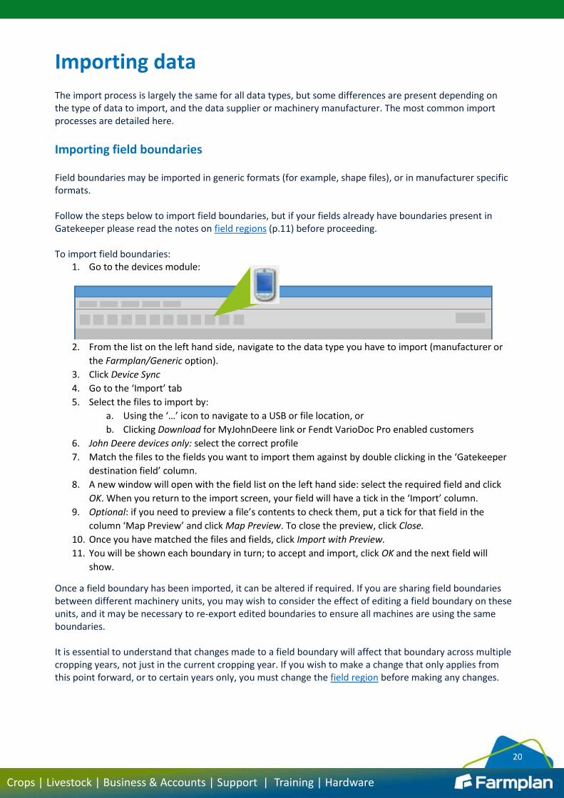
1. Go to the devices module:

2. From the list on the left hand side, navigate to the data type you have to import (manufacturer or

the Farmplan/Generic option).


4. Go to the ‘Import’ tab

5. Select the files to import by:

a. Using the ‘…’ icon to navigate to a USB or file location, or

b. Clicking Download for MyJohnDeere link or Fendt VarioDoc Pro enabled customers

6. John Deere devices only: select the correct profile

7. Match the files to the fields you want to import them against by double clicking in the ‘Gatekeeper

destination field’ column.

8. A new window will open with the field list on the left hand side: select the required field and click

OK. When you return to the import screen, your field will have a tick in the ‘Import’ column.

9. Optional: if you need to preview a file’s contents to check them, put a tick for that field in the

column ‘Map Preview’ and click Map Preview. To close the preview, click Close.

10. Once you have matched the files and fields, click Import with Preview.

11. You will be shown each boundary in turn; to accept and import, click OK and the next field will

show.

Once a field boundary has been imported, it can be altered if required. If you are sharing field boundaries between different machinery units, you may wish to consider the effect of editing a field boundary on these units, and it may be necessary to re-export edited boundaries to ensure all machines are using the same boundaries. It is essential to understand that changes made to a field boundary will affect that boundary across multiple cropping years, not just in the current cropping year. If you wish to make a change that only applies from this point forward, or to certain years only, you must change the field region before making any changes.

21


Importing field guidance, features, or zones Field guidance and feature data are generally imported from manufacturer specific file types after being collected on an in-cab or handheld controller. They may be imported to the field guidance and feature layers in Gatekeeper as appropriate. Gatekeeper can be used as a tool to store guidance data, and to share it between different machines on farm (including between different manufacturer formats). This also means it can be useful for sharing field data with contractors. Field zones are typically supplied in generic formats (for example, shape or ISOXML files), often contain field scale information such as soil types, and may be imported to Field Zones All Years or Field Zone Cropping Year layers. Any data imported to a field zone layer will replace any data already on that layer, it will not be added to existing data. Particular care must be taken to ensure you do not overwrite any field zone data. Data imported in any of the following steps can be viewed through the field or farm map by opening the appropriate layer.

Importing field guidance From the devices screen, with the correct device selected on the left hand side:


2. Check options on the device tab






6. Optional: if required, restrict the data shown in the import grid by selecting the data types you wish

to be visible, then click the green refresh icon beside the path to refresh the view

7. Depending on your setup, the files available to import may have already matched themselves to

the correct fields. If they have not, select fields by double clicking in the Gatekeeper destination

field column and select the correct fields.

8. Click Import with Preview

9. The fields will display one by one with the imported data visible. Click OK to accept and import.

Imported guidance data will always be stored on the field guidance layer ‘Imported Guidance’. For more information on managing guidance data, please see Managing imported field guidance (p.35).

Importing field features or zones From the devices screen:

1. Select the correct device from the left hand side, which will be either:

a. The specific manufacturer for the data files you have (for example, if features were scouted

using a Trimble handheld device, select the appropriate device from the Trimble options),

b. The specific data supplier of the data files you have (for example, if soil zones have been

created by RHIZA, select the appropriate device from the RHIZA options), or

c. The appropriate generic option from the section Farmplan/Generic > Field Zones/Features


3. Check options on the ‘Device’ tab


22







the correct fields. If they have not, select fields by double clicking in the Gatekeeper destination

field column and select the correct fields

8. Select the layer to import data on to by double clicking in the ‘Gatekeeper destination

zone/feature’ column. Please note:

a. Data must be matched to an appropriate layer type to display correctly – for example, if

you have scouted waypoints to import, the selected field feature layer should be ‘Scouted

Points’.

b. If importing data to field zone layers, remember that imported data will replace any

existing data on the matched layer, it will not be added to it. Take care not to over-write

any existing data.

9. When the required data is matched as required, click Import with Preview

10. The fields will display one by one with the imported data visible. Click OK to accept and import.

Imported field features or zones will be stored on the layer they were imported onto.

Importing soil sampling or field sensor data Use these steps to import soil sampling (nutrient analysis) data, field sensor data, or soil scanning where the data is supplied in a plot format. For soil scanning where the data is supplied as soil zones, please see Importing field features or zones (p.21). Data imported using the following steps may be viewed through the job map, and on the sampling tab of the field record. It will only be visible through the farm map if a corresponding geoanalysis layer is created. It is strongly recommended to create a plan to import sample and sensor data onto. The following steps assume that soil sampling has been carried out by a third party, who have provided results files for you to import into your Gatekeeper, or you are importing data from a field sensor. If you have carried out your own soil sampling by planning the sampling on Gatekeeper beforehand and now need to import lab results files, or by creating sampling grids in the field and now need to import both sampling grids and lab results files, please refer to Appendix 8 (p.71) for more detailed guidance. To create a sampling or sensor plan:

1. Open the planning module

2. Click Add Plan

3. Add a plan name, and select a plan group if required

4. Click Add Job >>

5. Select new job type ‘Field Sampling’

6. Click Add Field Sampling Job

7. Select field(s) as required

8. Select the data parameters that will be imported (for example, for soil sampling results select from

Soil Nutrients > P, K, Mg, pH. For soil scanning data, select from the heading group Field Sensor).

If you are not sure of all the parameters contained within the files, select at least one option at this

step so that the plan can be created; the additional data will still be imported and you may just

need to double check the headings selected after import.

23


Before clicking OK to select the data types: the order of sampling headings once they are selected

on the right hand side is the order they will appear in field records including reports. If you would

prefer them to appear in a specific order (for example, P, K, Mg, pH in that order) then click and

drag to rearrange sampling headings before clicking OK.

9. Click OK to save and close plan

10. Click Issue Plan, Issue Plan again, and then Close.

To import the sampling or sensor data to this plan:

11. Open the devices module

12. Select the correct device from the left hand side, which will be either

a. The specific data supplier of the data files you have (for example, if soil sampling results

have been supplied by SOYL, select the appropriate device from the SOYL options), or

b. The manufacturer of the field sensor, or

c. A user defined schema (for more information, please see User defined schemas [p.19])


14. Check options on the device tab. For import of field sensor data, make sure you select the correct

heading before proceeding.


16. Select the files to import by using the ‘…’ icon to navigate to a USB or file location

17. Match the first line of data to the plan by:

a. Double clicking in the Gatekeeper destination column

b. Selecting the correct plan from the list on the left hand side. If field names in the sampling

files match your Gatekeeper fields, clicking once on the plan will prompt Gatekeeper to

automatically find the correct field. If it does not match automatically, find the correct field

in the plan job.

c. Tick the option ‘Apply selected plan and best fit existing job to all following same type data

rows not selected for import’ to prompt Gatekeeper to try and match the rest of the

available files into the same plan

d. Click OK

18. If field names match then all lines should now have a tick in the ‘Import’ column. Select the field

and plan/job for any which have not been automatically matched


20. The plan will open with data imported to the fields as selected. To view fields, click on the Fields

tab, or click OK to accept the import and save.

Importing job records If you are importing work done as a record of field work, it is often easier to manage the data and import process if you have an issued plan to match job records back into. If you also have the ability to export work plans, it is strongly recommended to export a work plan to a device and then import work done into the same plan, and Gatekeeper will automatically match work back into an exported plan where possible. For more information, see Exporting work plans (p.45). If you already have an issued work plan, you will be able to match the completed work into it by following the steps below. However, you do not have to import files into an existing work plan. If no work plan is selected to match into at import, Gatekeeper will create a new plan as you import the files.

24


If you are importing data from a USB stick, you may wish to consider saving the files from the USB stick onto another location on your computer before proceeding. If you are importing harvest maps, especially to previous cropping years, please read Historic yield maps import mode (p.25) before proceeding.

Selecting implements Many types of data will require an implement to be present in the work plan, with a working width defined. To check whether your implements have working widths assigned, from the main Gatekeeper screen go to Setup > Implements and Settings. Implement management becomes increasingly important as you import and export precision farming data from Gatekeeper to machinery controllers. John Deere devices users should ensure they fully understand the implication of correct implement set up before proceeding – please see Appendix 5 (p.63) for further information.

Importing work done To import work records from a precision farming device:


2. From the list on the left hand side, select the appropriate device


4. Check the options on the devices tab – see Appendix 1 (p.52) for more information if required. If

you are importing jobs ‘on the fly’ rather than into a pre-existing plan, ensure you have the correct

import product matching mode selected, then click on the ‘Import’ tab



b. Clicking Download for MyJohnDeere link or Fendt VarioDoc Pro enabled customers.

6. John Deere Devices only: select the correct profile

7. Optional: if required, restrict the data shown in the import grid by selecting the data types you wish

to be visible, then click the green refresh icon beside the path to refresh the view


the correct fields and plan(s). If they have not, double click in the Gatekeeper destination field or

plan columns and select the correct fields and/or plans.

25


After matching the first field into the correct plan, Tick the option ‘Apply selected plan and best fit existing job to all following same type data rows not selected for import’ to prompt Gatekeeper to try and match the rest of the available files into the same plan

9. When the required data is matched as required, click Import with Preview.

10. Plans will open by job (so if you have matched into an existing plan with multiple jobs, you will only

see one job at a time).

Optional: if you created a new plan as you imported the data, you may wish to click on the plan tab

to enter a plan name and select a plan group.

11. Click OK to accept the data and import. If you have multiple jobs, the next job will show; repeat

until finished.

Matching data files to fields Where the data import option ‘Auto find job field by GK boundary is selected’, Gatekeeper tries to automatically match data to fields using the boundary as reference. Where data within a file falls into more than one field boundary, the data file is shown multiple times to allow the user to import the same file onto more than one field:

To preview the data in the file being duplicated, put a tick in the ‘Map Preview’ box and then click ‘Map Preview’. If ‘Auto find job field’ is not being used, and a file contains data for more than one field, it is possible to duplicate the data line so that it can be imported to multiple fields by:

1. Ticking the ‘Map Preview’ box for the file in question

2. Clicking Map Preview

3. Increase the number next to ‘Allocate plots to the additional number of fields’ as required

4. Click Close

5. Continue to import as required.

Historic yield maps import mode The historic yield map import option is designed to allow the import of yield maps to an existing harvest job. This most commonly occurs where either:

Harvested tonnages are recorded daily or regularly against fields throughout harvest, and maps are

matched onto these records after harvest is completed

Mapping and precision modules are added onto an existing Gatekeeper, and the user wishes to

backdate harvest records with combine maps.

It is necessary to use this option where harvest results already exist because otherwise each field will have offtakes recorded against it twice.

26


Due to differences in data manipulation available, use of this mode is not recommended unless necessary – in almost all cases, it is preferable to use the standard import option where possible. For further information please contact the support line who will be happy to advise on your particular circumstances.

27


Viewing imported data Following import, the location of data is dependent on the type of work or file imported. Imported field guidance or zones will be visible in mapping layers, while imported jobs will be visible through the planning or recording job, or field record.

Viewing imported work records When the import process is completed, the job details will be visible through the field record or planning module as usual. The associated jobs will be visible in the devices module and it is possible to double click to open the job to view or edit work records:

If the data imported contained field maps, there are two ways to view the maps once imported – through the field record, or through the work plan.

View a job map through the field record 1. Open the fields module

2. Click on the ‘Field’ tab

3. Click on the Field Map button

4. From the four vertical icons, click on the job data icon (green square and clipboard)

5. Expand the tree view to see the available spatial jobs for that field

6. Select the required job

7. Optional: select the way you wish to view the data from the ‘Displayed Job Data’ section of the job

data menu.

Advantages of viewing a map through the field record include the ability to compare other maps for the same field using the library map function.

View a sampling or sensor map through the field record 1. Open the fields module

2. Click on the ‘Sampling’ tab

3. If you have multiple types of sampling data: click on the appropriate subtab (i.e., soil, pest, tissue)

4. Double click on the map icon for a results map

Double click to open plan

28


5. From the four vertical icons, click on the job data icon (green square and clipboard) to view the

different sampling parameters and options for viewing them.

View a job, sampling map, or sensor map through the work plan 1. Either:

a. Open the planning module and select the required plan, double clicking to open, or

b. For job maps only: open the fields module and select a field. Click on the operations tab

and look for the plan (any job which has a map attached will have the map icon visible).

Double click to open the plan

2. From the fields tab of the plan, click the Field Map button (underneath the map)

3. From the four vertical icons, click on the job data icon (green square and clipboard)

4. Optional: select the way you wish to view the data from the ‘Displayed Job Data’ section of the job

data menu

5. Optional: it is possible to move between fields in the same plan by selecting them from the job data

menu.

6. Optional: place a tick in the box ‘All job fields’ at the top of the job menu screen to view all job

fields in one screen.

Advantages of viewing a map through the work plan include the ability to view different fields from the same job, or all job fields in one screen. Job and sampling maps can be viewed on the farm map after the creation of a geoanalysis layer (p.50).

Swapping job product or sensor headings If job data has been imported onto the wrong product or heading by accident, it is essential to use the steps below to allow the map data to be swapped onto the correct product without loss of data. Do not remove the product in question from the job and replace with another as any map and job completion data will be lost.

To swap an incorrect product 1. Open the plan in question

2. Click on the ‘Products’ tab

3. If there is more than one product in the job, ensure the product with the map attached to it is

selected on the left hand side

4. Click Swap

5. Select the correct product from the list and click OK


29


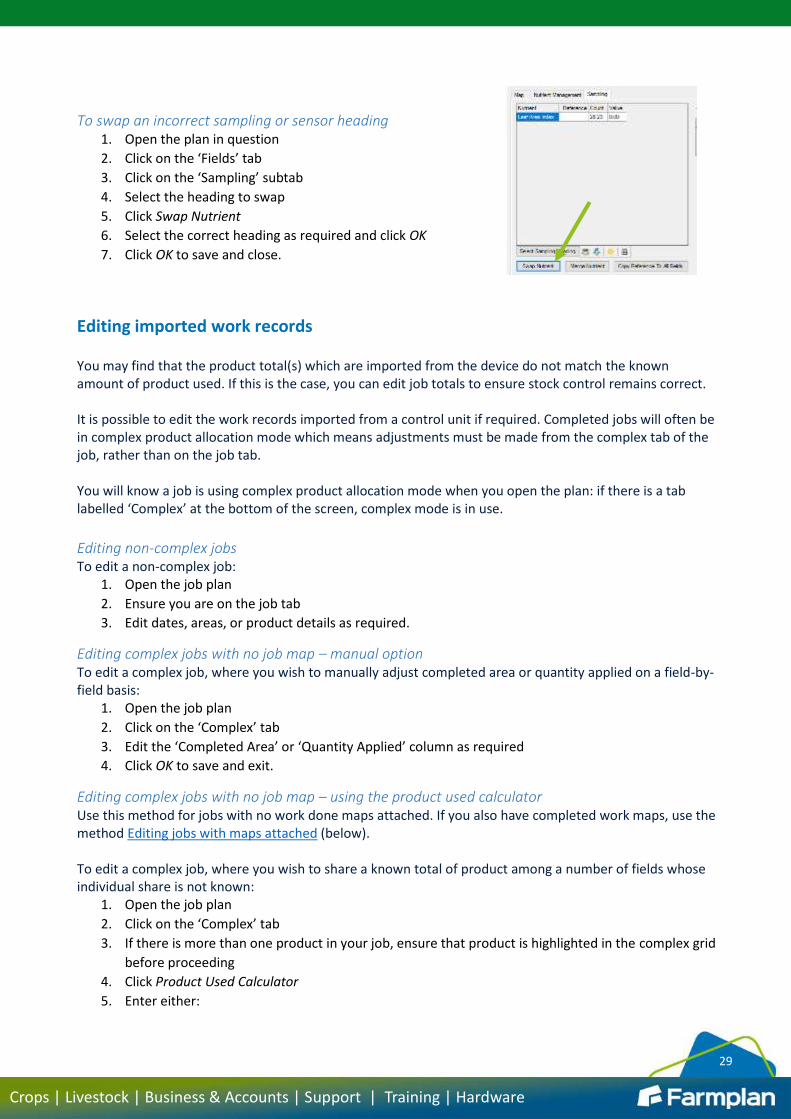
To swap an incorrect sampling or sensor heading 1. Open the plan in question

2. Click on the ‘Fields’ tab

3. Click on the ‘Sampling’ subtab

4. Select the heading to swap

5. Click Swap Nutrient

6. Select the correct heading as required and click OK


Editing imported work records You may find that the product total(s) which are imported from the device do not match the known amount of product used. If this is the case, you can edit job totals to ensure stock control remains correct. It is possible to edit the work records imported from a control unit if required. Completed jobs will often be in complex product allocation mode which means adjustments must be made from the complex tab of the job, rather than on the job tab. You will know a job is using complex product allocation mode when you open the plan: if there is a tab labelled ‘Complex’ at the bottom of the screen, complex mode is in use.

Editing non-complex jobs To edit a non-complex job:

1. Open the job plan

2. Ensure you are on the job tab

3. Edit dates, areas, or product details as required.

Editing complex jobs with no job map – manual option To edit a complex job, where you wish to manually adjust completed area or quantity applied on a field-by-field basis:


2. Click on the ‘Complex’ tab

3. Edit the ‘Completed Area’ or ‘Quantity Applied’ column as required

4. Click OK to save and exit.

Editing complex jobs with no job map – using the product used calculator Use this method for jobs with no work done maps attached. If you also have completed work maps, use the method Editing jobs with maps attached (below). To edit a complex job, where you wish to share a known total of product among a number of fields whose individual share is not known:


2. Click on the ‘Complex’ tab

3. If there is more than one product in your job, ensure that product is highlighted in the complex grid

before proceeding

4. Click Product Used Calculator

5. Enter either:

30


a. A new used rate

b. A new used quantity plus wastage quantity

c. A new total quantity

6. Select from the ‘Proportion Method’ section either:

a. ‘Area completed’, to allocate product share across fields by completed area

b. ‘Existing quantity used’ to allocate product share across fields by quantity used

7. Click Process

Editing jobs with maps attached – calibrating a job For harvest jobs with yield maps, please see Editing yield maps (p.30) before proceeding. The following steps will perform two functions at the same time: plot values within the map are adjusted to match the required total, and the total product used by the field (which relates to stock module) is adjusted. To calibrate a job map without affecting job product totals, ensure ‘New sub total quantity’ is not ticked at step 6. The following process may be carried out for single job records (e.g., one combine’s work where two were present in a field cutting at the same time), single fields, multiple fields, or all fields within a job:



3. Click Calibrate Job

4. Using the ‘Select’ column tick boxes, select either:

a. a single job line

b. all jobs for a field

c. multiple fields, or

Using the ‘Select All’ button underneath the grid, select all fields in the job

5. If your job has multiple products, select the correct product from the dropdown list at the top of

the page

6. Select the option ‘New sub total quantity’

7. In the box that appears, enter the quantity you wish to allocate to the selected field(s)

8. Ensure there is a tick in the option ‘Update job total quantity used’

9. Click Calibrate Plots

10. Repeat from 4 if necessary. Click OK to save and close.

Editing yield maps Harvest maps often need a small amount of editing after the import process to tidy up the data, and remove stray data points. This process should be done before harvest job quantities are adjusted (e.g., to match weighbridge figures).

The calibration function can be used to correct combine figures to weighbridge amounts, and also to adjust maps where two combines have been used in the same job with different factors

Calibrating data from more than one combine Where two combines have worked alongside each other with different calibration details, or different recording systems, this can result in a visible difference between the machines in yield maps:

31


Before opening the ‘Calibrate Job’ screen, you will need to identify which job line(s) relate to which part of the map image and require calibrating. From the fields tab of the harvest job, ensure you are viewing the map data in the ‘Actual Plots’ format. Each individual line you can see at this point is a separate data file from the combines:

Click on each data line to identify which part of the map they correspond to, and make a note of which line(s) relate to the data you need to calibrate, then:

1. Ensure you are not using a dynamic key to view the yield maps before proceeding. To view the key

in use:

a. Click ‘Field Map’ (underneath the visible map)

b. Go to the active tools menu

c. Check key visible in dropdown menu. If necessary, change to a fixed rate key. For more

information on mapping keys, please see Map Keys (p.13).

d. Click OK to return to the fields tab.

2. Click Calibrate Job

3. Using the ‘Select’ column tick boxes, select the data line(s) you wish to calibrate.

4. Depending on the combine type, there may be more than one option at this stage. Select from:

a. If the column ‘Calibration’ is present:

32


i. Each data line will have a calibration factor. The calibration factor is specific to the

machine and the settings at the time of cutting so the actual figure present doesn’t

matter. Matching calibration figures between machines will not necessarily match

the map data, but adjusting the calibration figure of the data lines required up or

down will allow you to ‘match’ one combine’s maps to the other.

ii. Select the method option ‘Calibration factor’

iii. Enter a new calibration factor in the box that appears

b. If the column calibration is not present:

i. You will need to adjust the line(s) required by adjusting the tonnages present in

‘Plot Quantity T’. Do not worry at this stage about correcting the tonnages to

known harvested amounts, this will be done in a separate step.

ii. Select the method option ‘New sub total quantity’

iii. Enter a new sub total quantity to adjust the selected records to

5. Click Calibrate Plots

6. Close calibration screen and check the visible map to see if maps have evened up. Repeat steps 2-5

as required until you are happy to proceed.

7. The process so far has corrected the map data so that the map trends as a whole are more robust.

It is now necessary to adjust the field’s tonnage to ensure that the data is more accurate to

offtakes, and to ensure stock levels (and therefore margin figures) are correct. To calibrate the

whole field for yield:

a. Click Calibrate Job

b. Select all records for the field in question

c. Select method option ‘New sub total quantity’

d. Enter the field’s weighbridge or total tonnage figure

e. Ensure there is a tick in ‘Update job total quantity used’

f. Click Calibrate Plots


Filtering and deleting plots Filtering plots allows data plots to be removed from the active map data. The functionality is most commonly used to remove data points which are the effect of how the combine was driven, rather than a true reflection of crop performance.

Raw data, plots and filled contour map Filtered data, plots and filled contour map

33


Filtering temporarily hides the plot and its associated data. It will not appear in maps, or be referenced by the grid generator if any application maps are made based on it, but it may be reinstated at a later date if required by adjusting the filters.

Deleting points permanently and irreversibly removes them from the map. This method is useful for removing plots which fall outside a field boundary, or which cannot be removed using filters. If points are deleted it is often advisable to recalculate the job data to take account of this change.

To filter job plots Filtering takes place within the plan job. To filter plots:



3. Click Filter Plots

4. If you have used plot filters before, select the filter template you wish to use from the list on the

left. If this is the first time you have used plot filters:

a. Click Add

b. Enter a filter name (e.g., ‘Wheat’)

c. Tick to activate any plot filters you wish to use, and enter the parameter required. For yield

maps, min and max rate and a start of pass delay are a good place to start. A description of

filter functions can be found in Appendix 3 (p.55).

5. If you have multiple products in the job (including a fixed cost product), check the correct product

is selected to filter.

6. If you do not wish to filter all fields in the job with these parameters, select the field(s) to filter from

the list on the right.

7. Click Filter Plots

The plots falling outside your specified parameters will now be hidden, and on the map have been replaced by an empty grey circle. Check the map and whether you wish to adjust the filter parameters. To re-filter, simply repeat steps 3-7 above, adjusting parameters as required. To re-instate all plots and remove the effects of a filter, click Filter Plots and then the button Use All Plots.

To delete all points outside of a field boundary This method is particularly useful where two fields have been cut in one work file, to quickly remove the data points not related to the field in question:

Raw data shows all captured plots Filtered data removes machinery effects to display field trends

34




3. Select the required field from the list on the left hand side

4. Click Field Map (long button underneath the field map)

5. Select the clip points tool (purple circle and scissors)

6. Make a single left click inside the field (a purple box will appear around the field and plots)

7. Right click and select the option Clip points outside field

8. Click Yes to the warning message

9. Click OK to close the mapping window

10. Click Recalc total quantities to ensure the plot and job values are updated.

To manually delete plots 1. Open the planning module and the plan required


3. Select the required field from the list on the left hand side

4. Click Field Map (long button underneath the field map)

5. From the tools:

a. To delete a single plot, select the delete point tool (purple circle and red cross). Left click on

a plot to select it, and left click again to delete.

b. To delete a series of plots, select the clip points tool (purple circle and scissors). Left click

once to select the field, and again to start drawing around the plots you want to delete.

Keep left clicking to draw a polygon around the plots you wish to delete. Right click and

select ‘Delete points inside polygon’.

6. Click OK to close the mapping window

7. Click Recalc total quantities to update plot and job values.

If you use the clip points tool at 5b: points are clipped according to the position of their co-ordinates (displayed as a snap point in the centre of the data point) to the polygon you draw. Therefore any points whose snap point is inside the polygon drawn will be deleted – you do not need to trace the exact outline of the plots. The example below shows plots around a pylon in the field being removed:

Data points to be removed

Snap points visible at centre of plot

Clip plots polygon drawn

Data points removed from map

35


Managing imported field guidance Imported field guidance is always stored on the field guidance layer ‘Imported Guidance’, and may be viewed through either the farm or field map.

To move a guidance line to another layer The following steps will move a stored guidance line off one layer onto another – not duplicate it:

1. Open the field or farm map as required

2. Select the layer ‘Imported Guidance’

3. Ensure the guidance layer is on top

4. Select the AB Line Data tool

5. Click on a snap point of the guidance line to move

6. In the screen that appears, select the new layer in the heading drop down list:


36


Creating variable rate maps Variable rate maps may be created in two main ways. The first of these is to manually draw areas onto a map and specify the rate of products to apply. This option is more suitable for creating a one-off map for a small number of fields, or maps which do not refer to multiple sources. The second is to use the grid generator to refer to multiple data sources and perform a set of pre-specified calculations. This option is suitable for creating maps for many fields at once using a similar rule-set, or for creating a map which refers to many different sources to create one application. It is possible to create a job with variable application jobs for more than one product, but extra steps must be taken as the job is created, and compatibility will depend on manufacturer specifications, so please contact the support line for further advice if required,

Manually creating a variable application map

1. Open the planning module

2. Click Add Plan

3. Enter plan name, select group if required, and click Add Job

4. Click Add Field Operation Job

5. Select field(s) as required

6. Select product. If most of the field will receive one rate, enter this rate. If there is not a rate for the

majority of the field, make the rate 0. Click OK

7. Select an implement


9. Click on the ‘Map’ subtab

10. Tick the option ‘Provide variable application target maps for ALL fields in this job’

11. Click Field Map (long button underneath the field)

12. Optional: if you want to refer to another mapping layer (eg a field zones layer), or the Bing maps

backdrop, ensure this is turned on through the layers menu before proceeding.

13. Select the active tools menu from the left hand side

14. Select the polygon tool (octagon) (other mapping tools may be used if required)

15. Above the mapping key, there is now a box where you can enter a rate. Type the rate you wish to

assign on the map

16. Left click around the area you wish to give this rate. You do not need to be too tidy around the field

boundary – the cells will not be filled beyond any cell which the boundary passes through.

17. When you have drawn the area, right click and select Finish this Entity

18. If required, repeat steps 15-17 for any other rates and areas.

19. If you have multiple fields, move on to the next field by selecting the job data menu and picking the

next field from the left. Repeat steps 14-18.

20. When all fields have application maps, click OK to save and close the mapping window

21. You will be returned to the plan. If you entered a rate of 0 at step 6, click on the job tab adjust the

job target rate so that it is not 0. The actual rate entered doesn’t matter and won’t adjust the maps

drawn, but certain rate controllers can’t accept maps with a target rate of 0.


The totals of products required by the maps you have just drawn may be viewed on the products tab. If you wish to adjust these totals (for example, to better fit seed totals or loads, see Adjusting map totals (p.37)

37


To print a job sheet which includes job maps, see Creating job sheets with maps (p.44) To export the variable plan, see Exporting work (p.45).

Adjusting map totals It is possible to bulk adjust the product totals required by a set of variable application maps. This can be useful to make sure that maps do not exceed the total amount of product available, or to better fit jobs into full loads or bags. To adjust the product totals of all maps within a job, from the fields tab:

1. Click Map Grid Options

2. Select the option ‘Proportion target rates to sum to a total quantity required’

3. In the text box that appears, enter the product amount you want the maps to add up to

4. Click Recalculate

5. Click OK

To adjust the product totals of one field within a job, or each field individually: from the fields tab, 1. Click Map Grid Options

2. At the top of the page, unselect any fields you do not wish to adjust

3. Click ‘Proportion target rates to sum to a total quantity required’

4. In the text box that appears, enter the product amount you want the map for that field to add up to


6. Repeat steps 2-5 for other fields as required

7. Click OK

Creating variable rate maps using grid generators The target grid generator function allows you to setup a rule (or combination of rules) which refer to different pieces of information held within Gatekeeper, and create a variable rate map. Although it takes a little time to set up a grid generator, the advantage is the speed with which it is possible to create maps for many different fields. Grid generators are made up of a number of different components:

Component Function Example Notes

Computation

Looks up a specific piece of information, and carries out a specified calculation based

on it

A computation could look for soil type zones in a field zone

layer, and apply a specific seed rate to each soil type

A grid generator may contain multiple computations,

referring to different pieces of information

Final adjustments

After computation(s) are carried out, final

adjustments may be applied to any rates calculated

A maximum rate may be set to cap any rates calculated

by computations

Final adjustments are always carried out in the order they

are listed on the screen

Fertiliser options

After all computation(s) and adjustment(s) are carried

out, any fertiliser options are applied

After calculating nutrients required based on soil

sample results, the grid generator can subtract any nutrient already applied in that year before finalising

the application map

For fertiliser jobs only – these options allow the user

to specify nutrient and conversion requirements.

Fertiliser products must be set up with nutrient

contents.

38


Due to the many different functions that grid generators can be used for, there are many combinations of options which may be used when creating a grid generator template. The first set of steps describes the general process, and then there are examples to show the most common options used.

Please be aware that the grid generator looks either to your own Gatekeeper data, or to imported customer field records, separately and as specified when the grid generator is set up. If your records contain data published from another Gatekeeper user, you will need to indicate when the data to compute has been imported by using the ‘Use Imported Customer Field Records only’ tick options as appropriate.

Setting up a grid generator template From the main Gatekeeper screen, go to Setup > Mapping > Grid Generator Templates and then:

1. Click Add

2. Name the new grid generator template

3. Select a template group from the dropdown list

4. Click Save

5. Click on the ‘Computations’ tab

6. Optional but recommended: in the ‘Reference’ box, type a description of your computation.

7. From the ‘Type’ dropdown list, select the kind of information you want the computation to lookup.

8. Specify the lookup data.

9. Specify the calculations to carry out when the lookup data is found.

10. Add any final adjustments required.

11. Add any fertiliser options required.


Grid generator template worked example: seed map based on soil zones The following steps are based on an example where:

The soil zones are saved on the Field Zones All Years layer ‘Soil Types’

The soil zones to be referenced are ‘Light sand’, ‘Medium’, and ‘Heavy Clay’

Each soil zone will have a specific rate in kg/ha set

From the main Gatekeeper screen, go to Setup > Mapping > Grid Generator Templates and then:

1. If this is the first grid generator you are adding, a new template named ‘New’ will be added

automatically; if it is not the first grid generator, click Add.

2. Name the template (e.g., ‘Winter wheat from soil zones’)

3. Select the template group ‘Seed’

4. Optional but recommended: add a brief description of the grid generator into the comment box


6. Edit the computation reference to ‘Soil zone lookup’

7. From the computation type dropdown list, select ‘Field Zones All Years’

8. Ensure the target job unit is ‘kg’.

9. At the bottom of the page, click Add Band to add the first calculation

10. Double click in the ‘Heading Group’ column and select ‘Soil Types’. The heading will automatically

be filled with the same name.

11. Double click in the ‘Zone Name’ column and select the first zone name you wish to reference (e.g.,

‘Light sand’)

12. In the ‘Action column’, select ‘Fixed Rate + Quantity’

13. In the ‘Quantity’ column, add the amount of seed to be applied anywhere the soil type is light sand

14. Repeat steps 9-13 for soil types medium and heavy clay, remembering to save.

15. Click on the ‘Final adjustments’ tab

39


16. Apply any final adjustments required: for drilling maps it is often a good idea to use ‘Default cell

rate given to all non calculated cells’ to make sure there are no 0 rate cells that would shut the drill

off.


Grid generator worked example: add a second computation to reference another feature The following steps illustrate how it is possible to use a grid generator template to refer to more than one field feature when creating a variable rate map. They are based on the additional example where:

The Field Zones All Years layer ‘All Years Management’ has a zone named ‘Headland’ added

All fields requiring an additional headland adjustment to seed rate have had a 12m headland drawn

in

All fields with a headland adjustment marked require an additional 25kg/ha seed to be applied.

Follow the steps above, and after step 14:

a. Click Add Computation

b. Edit the computation reference to ‘Headland adjustment’

c. From the computation type dropdown list, select ‘Field Zones All Years’

d. Ensure the target job unit is ‘kg’.

e. Ensure the computation summing type has ‘Add calculated rate’ selected

f. At the bottom of the page, click Add Band to add the first calculation

g. Double click in the ‘Heading Group’ column and select ‘All Years Management’. The

heading will automatically be filled with the same name.

h. Double click in the ‘Zone Name’ column and select the zone ‘Headland’

i. In the action column, select ‘= Fixed Rate’

j. Enter 25 into the fixed rate box (above the band)

k. Return to step 15 above.

Grid generator worked example: fertiliser map based on soil sampling results (+ optionally, refer to previous year’s yield maps) Based on an example where:

the nutrient being calculated for is P2O5

the soil sample results are being referenced as mg/L values

the yield map from last year was a winter wheat crop

From the main Gatekeeper screen, go to Setup > Mapping > Grid Generator Templates and then: 1. If this is the first grid generator you are adding, a new template named ‘New’ will be added

automatically; if it is not the first grid generator, click Add.

2. Name the template (e.g., ‘Phosphate VR application’)

3. Select the template group ‘Fertiliser’

4. Optional but recommended: add a brief description of the grid generator into the comment box


6. Edit the computation reference to ‘P lookup’

7. From the computation type dropdown list, keep ‘Previous Job (low start)’ selected

8. Under the ‘Bands’ section:

a. Select the lookup type ‘Sample Job’

b. Change the lookup years to ‘Look back starting this cropping year’

c. For lookup item, select ‘P’ from the list

9. Click Add Band

40


10. Enter the required calculations for the phosphate lookup. For example, if you wish to apply a

different rate based on soil index:

a. Double click in the ‘Action’ column and select ‘= Fixed Rate’

b. In the ‘From’ and ‘To Less Than’ columns, enter the lowest and highest mg/L value for index

0

c. In the ‘Target Grid Fixed Rate’ column, enter the amount of P2O5 to apply for index 0

results

d. Repeat steps 10 and 11 for index 1 and index 2.

Steps 11-18 are optional, to add a further computation which looks up the results of last year’s yield map and replaces the P offtake of that crop – if you do not wish to do this, continue to step 19.

11. Click Add Computation

12. Edit the computation reference (e.g., ‘Wheat yield’)

13. From the computation type dropdown list, keep ‘Previous Job (low start)’ selected

14. Change the ‘Lookup job unit’ to ‘t’ (assuming your primary outputs are setup with a default unit of t

not kg).

15. Under the ‘Bands’ section:

a. Keep the lookup type ‘Yield Job’

b. Change the lookup years to ‘Single year 1 ago’

c. Keep the lookup item ‘Wheat Winter’

16. Click Add Band

17. Enter the required calculations for the yield map lookup. For example, to apply 8.4kg of P2O5 per t

of crop removed:

a. Leave the ‘From’ value as 0, and add a ‘To Less Than’ value that is higher than any

reasonable crop yield (e.g., 20).

b. Keep the action as ‘Fixed rate + formula’

c. Change the method to ‘Lookup job kg * quantity’

d. Enter 8.4 in the ‘Quantity’ column.

18. Repeat 11-17 for other crops for which there is a yield map in the previous year.

All users:

19. Optional: Click on the ‘Final adjustments’ tab and enter any adjustments required. Useful options

for fertiliser grid generators include:

a. Zero the cell rate for all cells with a rate less than or equal to – set a minimum rate of

nutrient and any rates calculated below this will be replaced with a 0 rate. It can be useful

to enter the minimum theoretical rate your spreader or sprayer is capable of applying here

to make sure your map does not include rates the equipment cannot physically apply.

b. Lower rate limit applied to all non zero cells – the opposite of the ‘zero the cell rate’ option,

if you enter a number in here then any calculated rates below that number will be

increased to the number. Use this option if you would prefer to apply extra fertiliser rather

than cut back to 0 where low rates are calculated.

c. Upper rate limit applied to all cells – give a maximum application amount ceiling.

All calculations at this point for this example are in kg of nutrient, not product. Use the Agrilator if

necessary (press CTRL + A on the keyboard) to help move between nutrient and product.

20. Click on the ‘Fertiliser options’ tab.

21. In the ‘For the nutrient group’ dropdown list, select P2O5.

22. Place a tick in the option ‘Computations, final adjustments, and job default rate are all set up in this

template as nutrient rate’.

41


23. Optional: if you want the grid generator to take into account any fertiliser applications within the

current cropping year and take the applied nutrient off the calculated nutrient requirement

amount, place a tick in the option ‘Calculate the nutrient already applied this year’.


Screenshots of the grid generator examples here are available for cross reference in Appendix 4 (p.56).

Applying a grid generator to create a job with application maps Once the grid generator is created, go to the planning module and create a plan as usual. When you are returned to the main plan screen:


2. Select the ‘Map’ subtab (near the top of the page)

3. Put a tick in the option ‘Provide variable application target maps for ALL fields in this job’

4. Click Target Grid Generator

5. Select your grid generator template from the list on the left hand side

6. If your variable rate plan includes a fertiliser product and your grid generator is setup in rates of

nutrient, ensure you can see the product details in the ‘Fertiliser Product Nutrient Analysis’ box.

7. Click Generate Target Grid

8. Check the contents of the ‘Map Grid Generator Log’ window before closing.

There must be a logged count for every calculation you have asked the grid generator to carry out.

Gatekeeper does not warn you if it does not find a specified data field.

9. Click OK to close the grid generator screen.

Each field will now have a variable rate map visible; you can make manual adjustments or adjust the map totals as required, and export to variable rate controllers.

Making manual adjustments to a variable application map After you have used a grid generator, it is possible to make manual adjustments to a map if required. Common examples of when this would be suitable include to make a one-off adjustment to a map (to increase or decrease a rate based on a parameter you don’t want to build into a grid generator), or to put a zero rate area over the location of an in-field trial. To make manual adjustments to a map, after running a grid generator:



3. Optional: if you want to refer to another mapping layer (e.g. a field zones layer), or the Bing maps

backdrop, ensure this is turned on through the layers menu before proceeding.

4. Select the active tools menu from the left hand side

5. Select the polygon tool (octagon)

6. Above the mapping key, there is now a box where you can enter a rate. Type the rate you wish to

assign on the map

7. Left click around the area you wish to give this rate. You do not need to be too tidy around the field

boundary if your cell is near the edge of the field – the cells will not be filled beyond any cell which

the boundary passes through

8. When you have drawn the area, right click and select Finish this Entity

9. If required, repeat steps 6-8.

10. If there are any other fields in the job that you wish to adjust, you can move between them by

clicking on the job data menu.

Take care not to re-run the grid generator after you have made any manual changes (including using the Adjusting map totals method shown below) as they will be lost.

42


Adjusting map totals It is possible to bulk adjust the product totals required by a set of variable application maps. This can be useful to make sure that maps do not exceed the total amount of product available, or to better fit jobs into full loads or bags. To adjust the product totals of all maps within a job, from the fields tab:


7. Select the option ‘Proportion target rates to sum to a total quantity required’

8. In the text box that appears, enter the product amount you want the maps to add up to


10. Click OK

To adjust the product totals of one field within a job, or each field individually: from the fields tab, 8. Click Map Grid Options

9. At the top of the page, unselect any fields you do not wish to adjust

10. Click ‘Proportion target rates to sum to a total quantity required’

11. In the text box that appears, enter the product amount you want the map for that field to add up to


13. Repeat steps 2-5 for other fields as required

14. Click OK

Importing a SHP prescription from a third party to export to another controller If you have a variable rate prescription from a third party source it is possible to import this into Gatekeeper as a target map. This may be so that you can export the job in another manufacturer specific format, or in cases where the application controller does not have the ability to create an applied map but you wish to be able to create a record of variable application. To import a SHP file as a target prescription:


2. From the list on the left hand side, select ‘Farmplan/Generic’ > ‘Target Data’ > ‘Target Grid Shape

SHP (WGS84)’. If you do not see an expanding tree view, ensure the filters ‘Manufacturer’ and

‘Type’ are selected above the device list. If you do not see a specific node, put a tick in the option

‘Show inactive and unused manufacturers, types and devices’ in the green panel.


4. On the ‘Device’ tab, you may wish to check the following settings:

a. The option ‘Move source to archive after import’ is ticked/unticked as appropriate (this

option will move the SHP file from the folder it is saved in)

b. The option ‘Auto find job field by GK boundary’ is ticked

c. Under ‘Import Product Matching Mode’, you can select ‘Use this single selected product’ to

access the product list and specify which product should be used. It is possible to change

this later in the process so this is not essential.

5. Go to the ‘Import’ tab

6. Use the ‘…’ selector by path to select where the SHP files are saved

7. If your fields have not automatically matched: double click in the ‘Gatekeeper destination field’

column and in the new screen that opens, select the correct target field

If your fields have automatically been matched: tick ‘Import’ for each file you wish to import


43


9. A new draft plan will open with the maps attached. There are a number of options you may wish to

consider:

a. Click on the ‘Plan’ tab and give the plan a name and/or plan group.

b. Select an implement (and tractor unit)

c. If you imported a large number of fields and wish to break them down into smaller jobs:

i. Click on the job tab

ii. Click Split Job

iii. Select the field(s) to move

iv. Click OK

v. A new job will be created with the selected field(s). If you wish to name the

individual jobs, click on the job header tab and enter the job name in the ‘Optional

job reference’ box

10. Click OK to save and close the plan.

You will now have a draft plan with the prescriptions attached to the fields. You can now issue this plan and export to a device as usual (see Exporting data, p.45), or use the target maps to create a proxy application map (see Using Auto Actual, p.49).

Swapping products on an imported prescription It is possible to swap the products on a prescription that has been imported from a third party. However unless the product swapped to has the same nutrient contents, you will need to adjust the product rates within the maps, so care must be taken to ensure that the correct conversions take place as outlined below.

Prescription is in… I want to create a map in… Scenario to use at step 4:

kg of nutrient kg of product A

kg of product kg of nutrient B

kg of product kg of a different product C

In all cases, you will need to know the nutrient content of any fertiliser products involved. To swap products of a prescription and also adjust the product rates so that nutrient rates are unchanged:

1. Open the plan for the prescription in question

2. Click on the ‘Products’ tab

3. Make a note of the total amount of product required in the ‘Outstanding Requirement’ box

4. Click Swap

5. Select the replacement product to be used by the map

6. Click OK

7. Follow one scenario below as decided by the table above:

A. Take the product total from step 3 and convert this into a required amount of product,

using the Agrilator if required (press CTRL + A on the keyboard, click Fertiliser, and enter

product nutrient percentage and nutrient figure [enter total required even though it asks

for kg/ha]). This is your new map total amount for step 8.

B. Take the product total from step 3 and calculate the amount of nutrient contained within it

using the following formula:

The new map total calculated is your amount for step 8.

C. Take the product total from step 3 and calculate the amount of nutrient contained within

it, using scenario B above. Then take this amount of nutrient, and calculate the amount of

44


the second product required using scenario A above. This is your new map total amount for

step 8.

8. Click on the ‘Field’ tab


10. From the options at the bottom of the page, select ‘Proportion target rates to sum to a total

quantity required’

11. In the box that appears, enter your new map total amount from step 4.

12. Click Recalculate.

13. Click OK to close the map grid options screen and return to the plan.

Creating job sheets with maps To create a job sheet for jobs which include variable rate jobs, there are two options.

To create a job sheet with individual maps for each field With the plan selected in the planning module:

1. Click Reports

2. From the left hand side, select the report template ‘Work Plan Field With Maps’

3. Adjust any report options as required. If the Bing map backdrop was switched on last time you had

a mapping window open, it will display in the job sheet. To save ink you can switch it off by going to

the ‘Mapping’ tab and unticking the option ‘Show as backup layers in all maps’

4. Click Run Report

5. Save or print as required.

To create a job sheet with one map for all fields in a plan With the plan selected in the planning module:

1. Click Reports

2. From the left hand side, select the report template ‘Work Plan Farm Map’ or ‘Work Plan Farm Map

Landscape’

3. Optional: if your plan has multiple jobs, you can create a map per job (instead of a map per plan) by

unticking the option ‘Show data for all jobs in one map’. This is particularly useful where different

jobs contain blocks of fields which have distance between them.

4. If it is the first time you have used this report:

a. Click on the ‘Mapping’ subtab

b. In the grid at the bottom of the page, tick the box in the column ‘Target Grid Cells’ for the first

map layer. The text ‘Top(1)’ will appear.

5. Click Run Report

6. Save or print as required.

45


Exporting work or data to a device The following steps assume you have already set up a device as required. If this is not the case, please see Adding devices (p.17) before proceeding.

Export field details, including field guidance if required: Use these steps to export farm structure (e.g., field groups and field names) to a controller. The steps are the same whether you are only wishing to send field names, or field names plus boundaries and/or guidance lines. To export farm and field details to a device:




4. Click on the ‘Export’ tab

5. Select the path to export by using the ‘…’ icon to navigate to a USB. (MyJohnDeere and Variodoc

link customers should not change the path)

6. Click on the ‘Fields’ tab and:

a. Select any field group(s) applicable, or tick ‘Select All’

b. Select any crop(s) applicable, or tick ‘Select All’

c. John Deere devices only: ensure crops are linked to John Deere crops

d. Device dependent: select any guidance to export, or tick ‘Select All’

7. Click on the ‘Lists’ tab and:

a. Tick the product lists applicable

b. Device dependent: select any machinery lists or templates to export

8. Click Export

9. MyJohnDeere and Variodoc link customers only: click Upload.

Export field zones or field boundaries as a generic format Use these steps to export field zones or boundaries:


2. From the list on the left hand side, select the appropriate node (for example, ‘Entity Shape SHP

(WGS84)’)



5. Select the path to export by using the ‘…’ icon to navigate to a USB

6. Select field group(s) to export

7. For field zones only: select the layer(s) to export

8. Click Export

Export a work plan To export work plans to a precision farming device:





5. Select the path to export by using the ‘…’ icon to navigate to a USB. (MyJohnDeere or Variodoc link

customers should not change the path)

46


6. Click on the ‘Fields’ tab and:

a. Select any field group(s) applicable, or tick ‘Select All’

b. Select any crop(s) applicable, or tick ‘Select All’

c. John Deere devices only: ensure crops are linked to John Deere crops

d. Device dependent: select any guidance to export or tick ‘Select All’

7. Click on the ‘Lists’ tab and:

a. Tick the product lists applicable

b. Device dependent: select any machinery lists or templates to export

8. Click on the ‘Plans’ tab and:

a. Select the plan(s) to be exported

b. If your plan contains a variable rate application map, ensure there is a tick in the option

‘Export job target maps’

9. Click Export

10. MyJohnDeere or Variodoc link customers only: click Upload.

47


Reporting on precision farming data

Printing or saving maps There are two ways to create a map document from the Gatekeeper mapping module, which can then be saved or printed as required. Alternatively, it is also possible to run a map report from the fields module, which can then be saved, printed, or exported as required.

Save or print the current view from the mapping window To save or print the map as it appears in the mapping window, use the ‘Print’ icon:

In the window that opens, the following adjustments can be made if necessary:

Save or print a map report from the mapping window The second option for printing and saving from the mapping window is to create a map report. This option can be particularly useful where you have multiple field groups, because Gatekeeper will automatically scale each page of the report to the extent of the fields in each field group. To access map reports, click ‘Reports’:

To specify scale zoom, click here. Alternatively, roll in or out with mouse to adjust map fit on page

Change map fit on page

Add map title

Tick to show or hide options

Add comment

box – will be displayed in bottom left

corner

To adjust the map

location on page, use

arrows

48


Select from the available options as required and then click ‘Run Report’.

Save or print a map report from the fields module If you would prefer to view maps on a field by field basis, the selection of ‘Field Map’ type reports available in the field module may be more useful. If you wish to create a map report that displays cartographic layers, you will need to ensure these layers are visible in the map window before following the steps below. Cartographic layer contents are not clipped to the field boundary, so any entity outside a field boundary but in close proximity will still be visible. To run a field map report:

1. Go to the fields module

2. Click Reports

3. Select a ‘Field Maps’ report from the list – e.g., ‘Field Maps (Full)’

4. Depending on the data to be displayed, either:

a. For job data maps (soil sampling, field sensor, yield maps, etc): Keep the job option ‘Job

data’ and select the data to be displayed on the map from the ‘Headings’ list

b. For geoanalysis layers: Select the job option ‘Geoanalysis and field data’

5. To determine how the mapping data should be displayed, click on the ‘Mapping’ subtab and:

a. Select tick box options as required to show or hide map scale, north arrow, Bing backdrops,

etc

b. For job data maps: Scroll the grid at the bottom of the page and select the display mode

required (for example, for yield maps, tick ‘Actual Filled Contours’)

For geoanalysis layers: from the grid at the bottom of the page, select the geoanalysis layer

to be displayed

6. To specify which fields should appear in the report, click on the ‘Options’ subtab and click ‘Selected

Fields’ to pick the fields required

7. Click Run Report

The options selected at step 5 will be remembered next time you run the selected report, so you will only need to follow step 5 in subsequent times if you wish to change the options selected.

Field margin maps The field margin map function references product prices and confirmed application maps to create a spatial record of financial variation across the field. Margin maps are automatically generated, and are accessed through the fields module: click on the Margin tab and then Margin Maps button. In the window that opens, select from:

Variable costs

Outputs

Gross margin

Fixed costs

Net margin

If desired, a whole farm margin map may be created using a geoanalysis user defined layer. For more information, see Geoanalysis layers (p.50).

The margin map requires a confirmed work map for any variable application jobs. There are two ways for this to be populated in the work record:

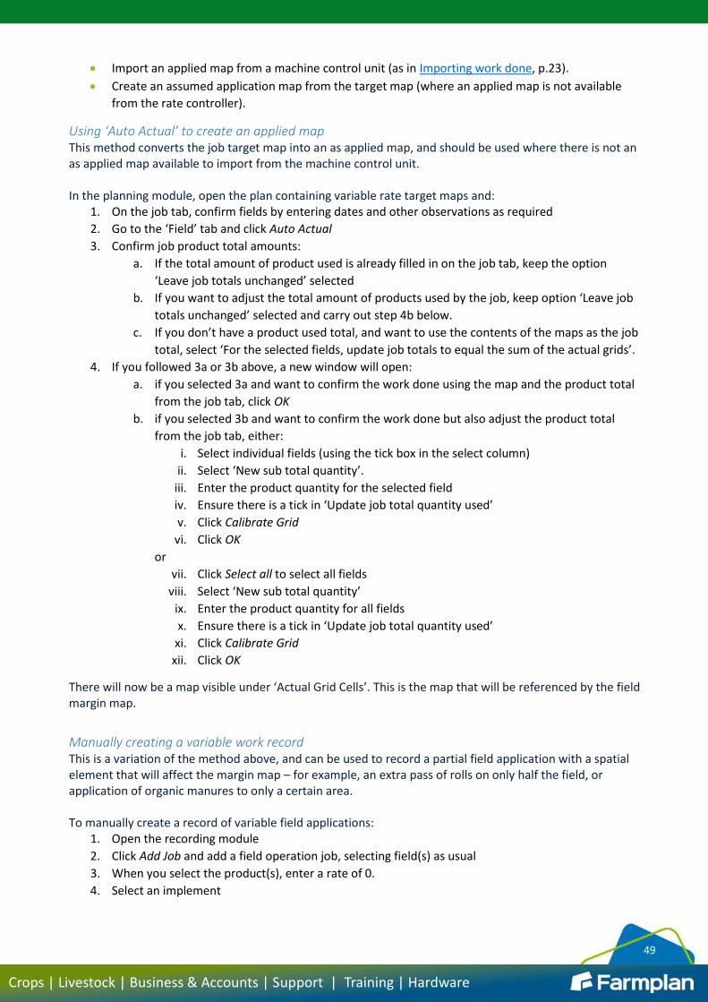
49


Import an applied map from a machine control unit (as in Importing work done, p.23).

Create an assumed application map from the target map (where an applied map is not available

from the rate controller).

Using ‘Auto Actual’ to create an applied map This method converts the job target map into an as applied map, and should be used where there is not an as applied map available to import from the machine control unit. In the planning module, open the plan containing variable rate target maps and:

1. On the job tab, confirm fields by entering dates and other observations as required

2. Go to the ‘Field’ tab and click Auto Actual

3. Confirm job product total amounts:

a. If the total amount of product used is already filled in on the job tab, keep the option

‘Leave job totals unchanged’ selected

b. If you want to adjust the total amount of products used by the job, keep option ‘Leave job

totals unchanged’ selected and carry out step 4b below.

c. If you don’t have a product used total, and want to use the contents of the maps as the job

total, select ‘For the selected fields, update job totals to equal the sum of the actual grids’.

4. If you followed 3a or 3b above, a new window will open:

a. if you selected 3a and want to confirm the work done using the map and the product total

from the job tab, click OK

b. if you selected 3b and want to confirm the work done but also adjust the product total

from the job tab, either:

i. Select individual fields (using the tick box in the select column)

ii. Select ‘New sub total quantity’.

iii. Enter the product quantity for the selected field

iv. Ensure there is a tick in ‘Update job total quantity used’

v. Click Calibrate Grid

vi. Click OK

or

vii. Click Select all to select all fields

viii. Select ‘New sub total quantity’

ix. Enter the product quantity for all fields

x. Ensure there is a tick in ‘Update job total quantity used’

xi. Click Calibrate Grid

xii. Click OK

There will now be a map visible under ‘Actual Grid Cells’. This is the map that will be referenced by the field margin map.

Manually creating a variable work record This is a variation of the method above, and can be used to record a partial field application with a spatial element that will affect the margin map – for example, an extra pass of rolls on only half the field, or application of organic manures to only a certain area. To manually create a record of variable field applications:

1. Open the recording module

2. Click Add Job and add a field operation job, selecting field(s) as usual

3. When you select the product(s), enter a rate of 0.

4. Select an implement

50


5. Enter a job date and any other observations required, except a product amount.


7. Click on the ‘Map’ subtab

8. Tick the option ‘Allow actual map data for THIS field and job’


10. Optional: if you want to refer to another mapping layer, or the Bing maps backdrop, ensure this is

turned on through the layers menu before proceeding

11. Select the polygon tool (octagon)

12. Left click around the area you wish to record an application for.

13. When you have drawn the area, right click and select Finish this Entity.

14. In the window that opens, enter the rate of product applied

15. Click OK

16. If required, repeat steps 13-16 for any other application areas

17. Click OK to save and close the mapping window

18. If required, repeat steps 8-17 for any other fields

19. Click Recalc Total Quantities

20. If your application was to a part field area, put a tick in the option ‘Also recalculate completed

areas’.

21. Click OK

22. Optional: if you want to adjust product totals to match a specific quantity:

a. Click on the ‘Job Header’ tab

b. Click on the ‘Proportion Method’ subtab

c. Select the option ‘Complex product allocation’

d. Click on the ‘Complex’ tab which will now be visible

e. Select from one of the following scenarios:

i. Where product quantities are known for each field: adjust the figure shown in

‘Quantity Applied’ column

ii. Where a total product quantity is known for the job: click ‘Product Used

Calculator’, enter total product quantity, select proportion method, and click

‘Process’


Creating whole farm geoanalysis layers The geoanalysis layers can be used to create whole farm versions of job maps – for example, whole farm soil sampling or yield maps.

The link between field records and geoanalysis layers is not ‘live’ – if you make any changes to field data, you must rebuild any geoanalysis layers for this change to be updated in the maps. Similarly, if you make any changes to the geoanalysis queries, you must rebuild the layer to update the map. All geoanalysis layers are specific to the cropping year they are in. When you move into another cropping year, the layer will be visible but will have nothing on it until you build it for the first time in that year by rebuilding the layer. While it may feel like more work than expected to create a query, once you have it set up you can use it year after year, so it will save time in the long run!

Creating a geoanalysis user defined layer to display job data Geoanalysis layers may be added in the farm map or field map, but are always generated for all fields (you cannot run a geoanalysis query on just one field).

51


To add a new geoanalysis layer, from either the farm map or field map window:

1. Select the geoanalysis menu from the left hand side

2. Click Add Layer

3. Enter a layer name

To create a new geoanalysis query: 1. Click Setup Queries

2. Click Add Query (or, if this is the first query you are creating, click Yes to the message that appears).

3. Enter a query name (we strongly suggest this is the same as the name you entered at step 3, so that

in future you know which query is for which layer).

4. Select query type option ‘Job data map’

5. Optional: if data to be displayed has been imported, tick ‘Use Imported Customer Field Records

Only’

6. Select map key to be used (use ‘…’ icon to link through to setup key window if you need to add or

edit a key before proceeding)

7. Click on the ‘Job data’ tab

8. Select the correct job type from the dropdown list. For example:

If building a whole farm yield map, select job type ‘Operations (cropping year)

If building a whole farm soil sample map, select ‘Sampling latest single job (multi year)

9. Sampling and sensing headings or multi-year queries only: select how many previous years’ data to

include in the map

10. Select the data to be displayed from the ‘Heading’ section (primary output, P index map, etc)

11. Check the options for summing method and source jobs

12. Select the map display options from the list on the right side of the screen. For some job types you

will only be able to select one option at this point (for example, for a yield map you can only select

one display option) but for others you are able to make more than one selection (for example, for

soil sample maps you can select filled contours plus actual text)

13. Click OK

To link the query to the layer and create the map:

14. Select the query you have just created from the dropdown list

15. Click Rebuild Layer

16. In the window that pops up, click OK.

The layer will be built. Depending on the amount of fields and data, this may take some time to process.

For a small selection of examples of geoanalysis layers and the queries used to create them, please see Appendix 7 (p.68).

52


Appendix 1 – device tab options Tick box options – select the options as required:

Option Function

Preview imported data by the job After clicking ‘Import’, user is shown a preview of the

job data with the option to cancel before the import is committing.

Job maps NOT to be saved Job maps are not imported, but other job data (times,

dates, etc) may be used to complete job records.

Move source to archive after import (specific devices only)

After complete import of the data in the source file, the file will be moved from its location into a

Gatekeeper archive location.

Clip job plots to field boundary

Any job plots which fall outside of the field boundary will be ignored and will not be imported to the job. Quantities attached to discarded plots are removed

from the product quantities.

Keep all out of work job plots Any plots marked as out of work by the implement are

imported to Gatekeeper.

Auto find job field by GK boundary Job plot location is used to try and automatically

identify the correct field by boundaries.

Historic yield maps import mode Allows the import of yield maps to an existing record

without adjusting stock levels – for more details please see Historic yield maps (p.25).

Work done uses outstanding field area

Completed job record uses the field working area as the job area, rather than the area recorded by the

implement (which can in some cases be larger than the field area, due to machinery overlaps).

Store job plot height data If job plot height has been stored by the implement,

import this data and store with the job.

Import product matching mode – select one option as appropriate:

Option Function

Use device file products matched to Gatekeeper products by their name

Product names as they appear in the device data are correct: new products will be created in Gatekeeper

stock if the exact product name as used on the device does not already exist in stock.

Any destination job products matched by their order override the device file product names

The products as selected in an existing plan are correct and should be used in preference to the product

names in the device data. This option requires a pre-populated plan for the data to be imported onto.

Use this single selected product Job should use the product selected at this point. This option is ideal if data is being imported ‘on the fly’ and

not matched into an existing plan.

Import width override: if required, adjust the default implement width (which will be reflected in plot widths on job maps), or override the plot width contained within the job data. Sensor import options: for any job record which contains a sensor map, select the heading for the sensor map to be stored under. If you will be collecting multiple crop maps throughout the season, they should be differentiated to allow later comparison. More headings can be added if required via Setup > Headings.

53


Appendix 2 – gridding methods

Gridding method Functionality Suggested uses

Application For display of imported application maps. Each cell is given the value of the plot nearest to its

centre. Imported application maps

Inverse distance

Suited only to maps which contain a lot of field data (e.g., yield maps or field sensor maps). The cell value is calculated as a weighted average of

points around the cell.

For custom inverse distance gridding methods, you can specify both the search area (how far

around the cell to look for data points) and the weighting power (the relative ‘strength’ of points closer or further away from the cell).

Maps with many data points – for example, yield maps

Kriging

Designed for when a smoothed map is required, but there are relatively few data points within

the map. The cell value is calculated based on a predicted trend between data points.

For custom kriging methods, the search area and the maximum number of plots to reference may

be specified.

Jobs with few data points where a smoothed map is

required – for example, soil sampling result maps

Nearest Neighbour

Cell value is the same as the nearest job data point to the cell. The value of cells between two different data points are not extrapolated based

on algorithms (compare with kriging)

Jobs with few data points where cell values should not be extrapolated – for example, soil

sampling maps which will be referenced to create an

application map

Sample Region

Designed for sample data where widely distributed data was collected on a regular grid

basis. Each job data point has a region surrounding it of half the distance between it

and the next point; any cell within a point region is allocated the sample result (no extrapolation

occurs)

Sampling jobs which were undertaken on a regular grid

basis.

Job Zones Override

Where job data was created with zones to accompany the job point data (most commonly soil sampling), the results of each plot is applied to the extents of the sampling zone to which it

belongs.

Soil sampling result maps where the sampling was based

on zones

Some examples of gridding methods and their effect on data display are shown below. These examples are strictly illustrative and are not intended to suggest that all gridding methods are suitable for use in all situations!

54


Example 1 – soil sample results map raw data

Nearest neighbour Kriging Sampling region Job zones override

Example 2 – yield map raw data

Inverse distance Nearest neighbour Kriging

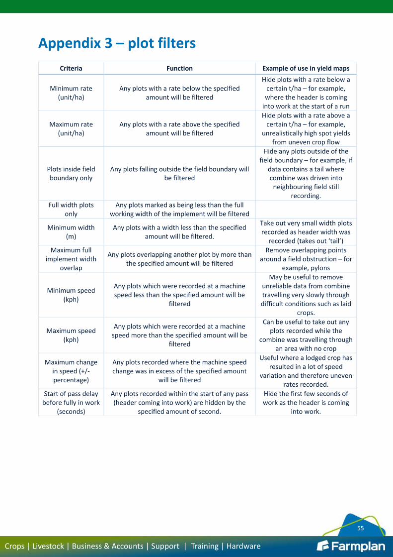
55


Appendix 3 – plot filters

Criteria Function Example of use in yield maps

Minimum rate (unit/ha)

Any plots with a rate below the specified amount will be filtered

Hide plots with a rate below a certain t/ha – for example, where the header is coming

into work at the start of a run

Maximum rate (unit/ha)

Any plots with a rate above the specified amount will be filtered

Hide plots with a rate above a certain t/ha – for example,

unrealistically high spot yields from uneven crop flow

Plots inside field boundary only

Any plots falling outside the field boundary will be filtered

Hide any plots outside of the field boundary – for example, if

data contains a tail where combine was driven into

neighbouring field still recording.

Full width plots only

Any plots marked as being less than the full working width of the implement will be filtered

Minimum width (m)

Any plots with a width less than the specified amount will be filtered.

Take out very small width plots recorded as header width was

recorded (takes out ‘tail’)

Maximum full implement width

overlap

Any plots overlapping another plot by more than the specified amount will be filtered

Remove overlapping points around a field obstruction – for

example, pylons

Minimum speed (kph)

Any plots which were recorded at a machine speed less than the specified amount will be

filtered

May be useful to remove unreliable data from combine travelling very slowly through difficult conditions such as laid

crops.

Maximum speed (kph)

Any plots which were recorded at a machine speed more than the specified amount will be

filtered

Can be useful to take out any plots recorded while the

combine was travelling through an area with no crop

Maximum change in speed (+/- percentage)

Any plots recorded where the machine speed change was in excess of the specified amount

will be filtered

Useful where a lodged crop has resulted in a lot of speed

variation and therefore uneven rates recorded.

Start of pass delay before fully in work

(seconds)

Any plots recorded within the start of any pass (header coming into work) are hidden by the

specified amount of second.

Hide the first few seconds of work as the header is coming

into work.

56


Appendix 4 – grid generator options

Data fields When building grid generator templates: the order of computations in the grid generator and whether they are set to add, subtract, or replace can make a huge difference to the functionality.

Job types

Job type Functionality Use for…

Previous job (low start)

Look for a previous spatial job; the bands entered will start with the

lowest rates found in the job. (Lookup rates are specified as

From – To Less Than)

Referencing the rates of a previous job record with map –

for example, yield maps, spatial soil sampling results, or

previous application maps Previous job (high start)

Look for a previous spatial job; the bands entered will start with the

highest rates found in the job. (Lookup rates are specified as

To Less Than – From)

Field Features Crop Year Looks for field feature polygons with text associated to them. If the text

matches text specified in a computation, the computation

action is applied

Look up sample point waypoints if stored on a field

features layer Field Features All Years

Field Zones Crop Year Look for zones within a field zones

cropping year layer

Looking up zones for a specific cropping year – the reference

year can be specified

Field Zones All Year Look for zones within a field zones

all years layer

Looking up perennial field zones – for example, soil type

zones

Lookup types

Job type Functionality

Application job Search jobs where product has been applied to fields – all variable cost

headings can be searched.

Sample job Search for results of a nutrient sample

Sampling difference Searches for the difference found between multiple nutrient sample

jobs

Sensing job Search for results of a sensor value

Sensor difference Search for the difference found between sensor jobs

Sensor normalised variation Search for the results of a normalised variation sensor map

Target yield (non spatial) Refer to the estimated target yield (as set in the cropping record). This

option is not inactivated by ticking the ‘Ignore jobs with no spatial data’ option.

Total nutrient applied Search jobs for the total amount of the specified nutrient applied

Weeds, pests and diseases difference

Search for the difference found between sample jobs where weeds, pests, and diseases have been recorded.

57


Weeds, pests and diseases job Search for the results of jobs where weed, pest, or disease sample

values have been recorded

Yield job Search for a yield job recorded to a field (spatial or non-spatial)

Yield normalised variation Search for the results of a normalised variation yield map

Actions

Action Functionality Use for…

= Fixed rate Applies the fixed rate specified

Applying a single value to a lookup criteria – for example, if

the soil type zone is ‘Sandy Loam’, apply 180kg/ha seed

Fixed rate + formula Applies the fixed rate (which can be

0) plus the formula specified Calculating a value based on

the lookup value of the reference map – for example,

when referring to tonnages in a yield map. Used in conjunction

with formulas, see below.

Fixed rate - formula Applies the fixed rate minus the

formula specified

Formulas

Formula Functionality

Lookup job value + quantity Add specified value to the value present in the

reference job map

Lookup job value - quantity Minus specified value from the value present in the

reference job map

Lookup job value * quantity Multiply result of the reference job map by a specific

value

Lookup job value / quantity Divide result of the reference job map by a specific

value

58


Example 1 – seed map from soil zones

Name entered

Group selected

Descriptive comment for future reference

Computation added

Description entered

Type is ‘Field Zones All Years’

Three bands added: Heading group = soil types

Heading = soil types [layer name] Zone names = [zones used]

Action = Fixed rate + quantity Quantity = rate to apply

Target job unit is kg

59


Computation added

Description entered

Type is ‘Field Zones All Years’


One band added: Heading group = All years management

Heading = All years management [layer name] Zone name = Headland adjustment

Add calculated rates selected

Fixed rate entered

Action = Fixed rate

60


Example 2 – fertiliser map from soil sampling and yield maps

Name entered

Group selected

Descriptive comment for future reference

Computation added

Description entered

Type is ‘Previous job (low start)’


Lookup years = look back starting this cropping year

Lookup type = Sample Job Lookup item = P

Three bands added. Lookup values specified

Action = Fixed rate Fixed rates entered

61


Description entered

Computation added

Type is ‘Previous job (low start)’

Target job unit is kg, lookup job unit is t

Add calculated rates selected

Lookup years = single year 1 year ago Lookup type = Yield job

Lookup item = Wheat winter

One band added. Lookup values specified Action = fixed rate + formula

Formula method = lookup job t * Quantity Quantity entered as required.

Minimum application rate specified (in kg of nutrient

not product)

Rate rounding specified

62


P2O5 specified as nutrient

Options to convert to product rate and reduce rates by nutrient already

applied ticked

63


Appendix 5 – John Deere devices There are additional specific settings which must be used when exporting to or importing from a John Deere unit. For more information on any of the processes below, please refer to the John Deere devices Quick Start Guide which can be accessed through Gatekeeper by clicking Help > Quick Start Guides, or from the Farmplan website training section.

Crops All active crops must be linked to a John Deere crop before export may take place. To link crops, from the main Gatekeeper screen:

1. Click Setup >Crops and Varieties

2. Select a crop from the left hand side (make sure you are at the crop not crop group level)

3. By the option John Deere Linked Crop, place a tick in the box to activate the dropdown list

4. Select the appropriate crop to link with.

5. Repeat for crops as required.

When you export jobs or data to a John Deere device, the linked crops must be selected on the field subtab of the export tab of the device sync screen:

Implements and tractor units It is essential that implements are imported from the unit before any work is exported. To import machinery settings:


2. Select the John Deere device node and click Device Sync

3. On the ‘Import’ tab, select the path using the ‘…’ icon

4. Select the correct profile

5. Look for the machinery file line (it will be yellow)

Unless all crops are correctly

linked and visible here, data cannot be exported

64


6. Put a tick in the ‘Import column’ and click Import with Preview

7. In the new window that opens, select the implement(s) and machine(s) you wish to import and

click OK.

Profiles When data is exported from a John Deere unit to the USB, a profile name is entered on the screen at the point of export. This helps users to identify which work is present within a particular set of files. When importing data from John Deere devices, the profile must be correctly selected before the data to import will be visible. When exporting data to John Deere devices, the name of the profile may be changed if required by selecting into the profile dropdown and over-typing the new, required profile name.

65


Appendix 6 – user defined import schema Worked example where EM scan data is provided in a .csv file

And the data required for import is:

Column A (job date)

Column D (point co-ordinate longitude)

Column E (point co-ordinate latitude)

Column F (point altitude)

Column M (conductivity shallow)

Column O (conductivity deep)

Schema type – Sampling job Schema sub type – Field sensor Implement width – if required Coordinate type – WGS84 [if correct] Delimiter - , (comma) [if correct]

Valid file extensions - .csv Merge with existing plots – no Zero value plots are valid – [as required]

66


Click to add header line, and then match columns – in this case, sample date.

Example file selected

Select data tab

For any columns with data to import, double click in ‘Import Column As’ row and select the data contained within

the column.

67


For columns with sample data to import, the column is identified as ‘Sample 01 Value’ and then the data heading

must be selected in the ‘Additional Data’ row. For example, to import altitude, Import Column As = Sample 01 Value;

Additional Data = Sample Height (m)

68


Appendix 7 – geoanalysis queries

Example 1 – whole farm yield map

Query type is ‘Job data map’

Map key selected

Job type is ‘Operations (cropping year)’

Heading is ‘Primary Output’

Map format is ‘Actual filled contours’

69


Example 2 – whole farm sampling results


Map key selected

Job type is ‘Sampling latest single job (multi year)’

Look back for appropriate number of years as required

Heading is ‘pH’

Source jobs set to ‘Only use jobs with spatial data’. Where fields have a mixture of spatial and whole field sampling, ‘Use all jobs’ may

be more appropriate

Map format is ‘Actual filled contours’ plus

‘Actual plot text’

70


Example 3 – normalised yield maps


Map key selected

Job type is ‘Yield normalised variation (multi year)’

Look back for appropriate number of years as required

Map format is ‘Actual filled contours’

71


Appendix 8 – soil sampling scenarios There are many variations on how Gatekeeper can be used to plan and/or facilitate soil sampling, as well as record the results of any sampling which has taken place. The following scenarios cover the most common options but are not exhaustive, so please contact the support line if you have any queries.

Planning sample zones Where field will be sampled in zones rather than at specific locations (waypoints):

1. Open farm map module

2. Go to layers menu

3. Select a field zones all years layer as appropriate (for example, soil sampling)

4. Put selected layer on top

5. Go to active tools menu

6. If this is the first time you have used the layer selected:

a. Click Select Zones

b. Click Pick Zone Names

c. Select from ‘Sampling Zones (01+)’ or ‘Sampling Zones (A-Z)’ the number of zones required,

select using the single right arrow, and click OK

d. Click OK to return to mapping

7. Draw zones as required, by either:

a. Drawing freehand, remembering that it does not matter if zones overlap, but that the top

zone has precedence, or;

b. Use the gridding tool to create regular zones:

i. Select gridding tool (# icon)

ii. Adjust size options if required – 100x100m grids gives ha sampling

iii. Ensure mode selected is ‘Sampling’

iv. Adjust offset if required (this affects how the grids are laid out into the field)

v. Double click in field to start drawing base line, left click to place end of line

vi. Grid will automatically populate within field. If required, grid may be edited at this

point (for example, you may wish to use ‘Change polygon zone’ tool to merge two

neighbouring cells)


Planning sample points Where field will be sampled at specific locations rather than in zones:

1. Open farm map module

2. Go to layers menu

3. Select a field zones all years layer as appropriate (for example, soil sampling)

4. Put selected layer on top

5. Go to active tools menu

6. To use the measuring grid tool to divide the field into regular portions:

a. Select measuring grid lines tool (# with ruler underneath)

b. Adjust size options if required – 100x100m grids gives ha sampling

c. Ensure mode selected is ‘Sampling’

d. Adjust offset if required (this affects how the grids are laid out into the field)

e. Double click in field to start drawing base line, left click to place end of line

f. Grid will automatically populate within field.

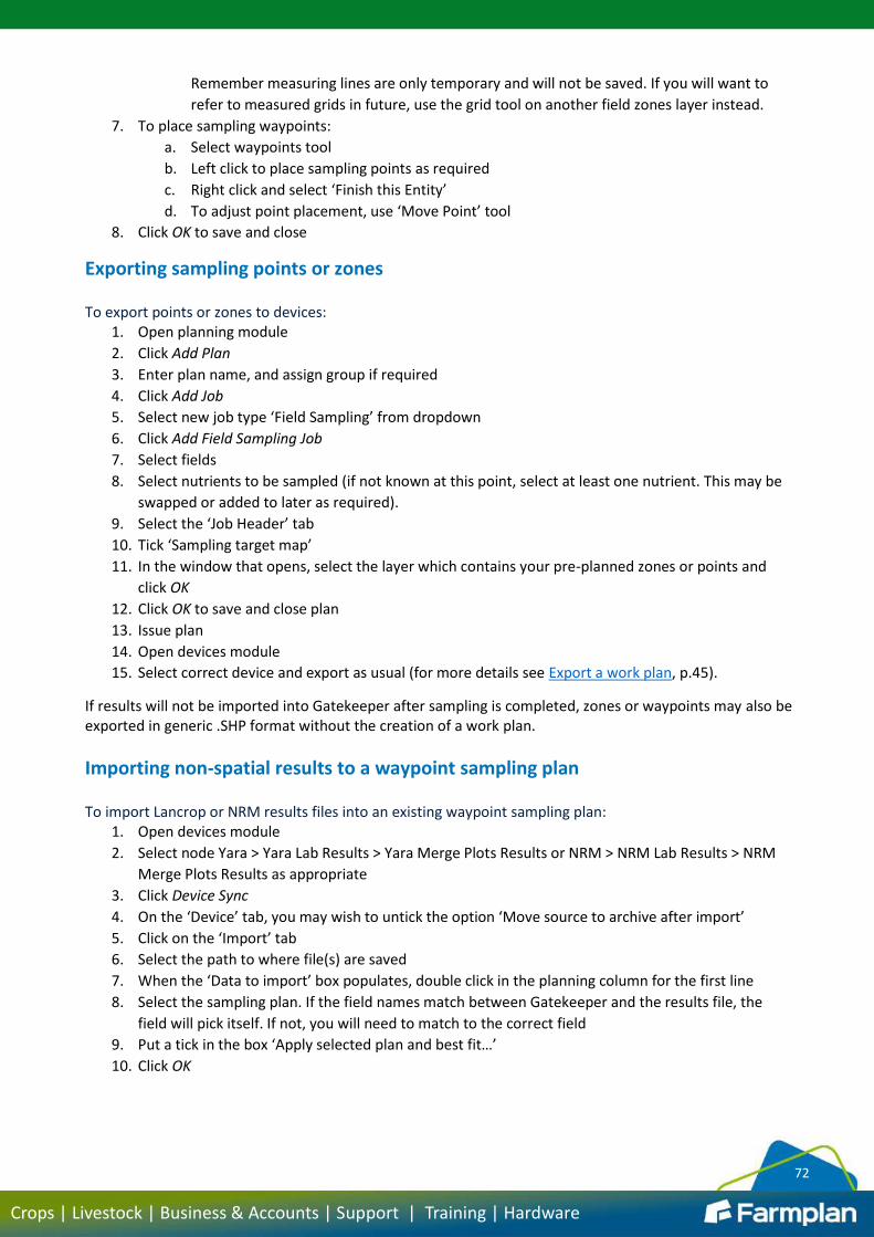
72


Remember measuring lines are only temporary and will not be saved. If you will want to

refer to measured grids in future, use the grid tool on another field zones layer instead.

7. To place sampling waypoints:

a. Select waypoints tool

b. Left click to place sampling points as required

c. Right click and select ‘Finish this Entity’

d. To adjust point placement, use ‘Move Point’ tool


Exporting sampling points or zones To export points or zones to devices:

1. Open planning module

2. Click Add Plan

3. Enter plan name, and assign group if required

4. Click Add Job

5. Select new job type ‘Field Sampling’ from dropdown

6. Click Add Field Sampling Job

7. Select fields

8. Select nutrients to be sampled (if not known at this point, select at least one nutrient. This may be

swapped or added to later as required).

9. Select the ‘Job Header’ tab

10. Tick ‘Sampling target map’

11. In the window that opens, select the layer which contains your pre-planned zones or points and

click OK

12. Click OK to save and close plan

13. Issue plan

14. Open devices module

15. Select correct device and export as usual (for more details see Export a work plan, p.45).

If results will not be imported into Gatekeeper after sampling is completed, zones or waypoints may also be exported in generic .SHP format without the creation of a work plan.

Importing non-spatial results to a waypoint sampling plan To import Lancrop or NRM results files into an existing waypoint sampling plan:


2. Select node Yara > Yara Lab Results > Yara Merge Plots Results or NRM > NRM Lab Results > NRM

Merge Plots Results as appropriate


4. On the ‘Device’ tab, you may wish to untick the option ‘Move source to archive after import’

5. Click on the ‘Import’ tab

6. Select the path to where file(s) are saved

7. When the ‘Data to import’ box populates, double click in the planning column for the first line

8. Select the sampling plan. If the field names match between Gatekeeper and the results file, the

field will pick itself. If not, you will need to match to the correct field

9. Put a tick in the box ‘Apply selected plan and best fit…’

10. Click OK

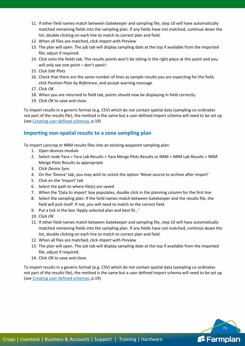
73


11. If other field names match between Gatekeeper and sampling file, step 10 will have automatically

matched remaining fields into the sampling plan. If any fields have not matched, continue down the

list, double clicking on each line to match to correct plan and field.

12. When all files are matched, click Import with Preview

13. The plan will open. The job tab will display sampling date at the top if available from the imported

file; adjust if required.

14. Click onto the fields tab. The results points won’t be sitting in the right place at this point and you

will only see one point – don’t panic!

15. Click Edit Plots

16. Check that there are the same number of lines as sample results you are expecting for the field,

click Position Plots by Reference, and accept warning message

17. Click OK

18. When you are returned to field tab, points should now be displaying in field correctly.


To import results in a generic format (e.g. CSV) which do not contain spatial data (sampling co-ordinates not part of the results file), the method is the same but a user defined import schema will need to be set up (see Creating user defined schemas, p.19)

Importing non-spatial results to a zone sampling plan To import Lancrop or NRM results files into an existing waypoint sampling plan:


2. Select node Yara > Yara Lab Results > Yara Merge Plots Results or NRM > NRM Lab Results > NRM

Merge Plots Results as appropriate




6. Select the path to where file(s) are saved

7. When the ‘Data to import’ box populates, double click in the planning column for the first line

8. Select the sampling plan. If the field names match between Gatekeeper and the results file, the

field will pick itself. If not, you will need to match to the correct field

9. Put a tick in the box ‘Apply selected plan and best fit…’

10. Click OK

11. If other field names match between Gatekeeper and sampling file, step 10 will have automatically

matched remaining fields into the sampling plan. If any fields have not matched, continue down the

list, double clicking on each line to match to correct plan and field.

12. When all files are matched, click Import with Preview

13. The plan will open. The job tab will display sampling date at the top if available from the imported

file; adjust if required.


To import results in a generic format (e.g. CSV) which do not contain spatial data (sampling co-ordinates not part of the results file), the method is the same but a user defined import schema will need to be set up (see Creating user defined schemas, p.19)

74


Importing spatial results To import files provided by a third party which contain the sample location or zones as well as the analysis results, follow the steps provided in Importing soil sampling or field sensor data (p.22).

Importing sampling waypoints Where waypoints were generated at the point of sampling and need to be imported into Gatekeeper:


2. Select correct import node




6. Select the path to where the file(s) are saved

7. When the ‘Data to import’ box populates, double click in the zone/feature column for the first line

8. Select the zone layer to import the waypoints onto. Remember any data imported onto a field zone

layer will replace any data already on that layer, not added to existing data. Ensure you have the

correct layer selected at this point before proceeding.

9. If the field names match between Gatekeeper and the results file, the field column will be matched.

If not, double click in the field column and select the correct field.


11. You will be shown each field in turn. Click OK to accept and import

To match analysis results to sampling locations, follow the steps in Planning sample points (p.71) and then Importing non-spatial results to a waypoint sampling plan (p.72).

Importing sampling zones Where zones were generated at the point of sampling and need to be imported into Gatekeeper:


2. Select correct import node




6. Select the path to where the file(s) are saved

7. When the ‘Data to import’ box populates, double click in the zone/feature column for the first line

8. Select the zone layer to import the zones onto. Remember any data imported onto a field zone

layer will replace any data already on that layer, not added to existing data. Ensure you have the

correct layer selected at this point before proceeding.

9. If the field names match between Gatekeeper and the results file, the field column will be matched.

If not, double click in the field column and select the correct field.


11. You will be shown each field in turn. Click OK to accept and import.

To match analysis results to sampling locations, follow the steps in Planning sample zones (p.71) and then Importing non-spatial results to a zone sampling plan (p.73).

precision farming modules - amazon web services

Documents