PRECIPITATION TENDENCIESPRECIPITATION TENDENCIES& DIAGNOSTIC PRECURSORS& DIAGNOSTIC PRECURSORS

IN THE UPPER DANUBE CATCHMENT IN THE UPPER DANUBE CATCHMENT PARALLEL TO GLOBAL WARMING PARALLEL TO GLOBAL WARMING (1974-2003)(1974-2003)

JánosJános MikaMika11, Vera Schlanger, Vera Schlanger11, , Blanka BartókBlanka Bartók22 & Gábor Bálint & Gábor Bálint33

11Hungarian Meteorological Service, Budapest, Hungarian Meteorological Service, Budapest,

22Babes Bolyai University, Cluj, RomaniaBabes Bolyai University, Cluj, Romania,,

33Water Resources Research Centre, VITUKI, BudapestWater Resources Research Centre, VITUKI, Budapestwith special thanks towith special thanks to Judit Bartholy & Rita PongráczJudit Bartholy & Rita Pongrácz,, Eötvös Loránd University, Budapest;Eötvös Loránd University, Budapest; Emőke BorsosEmőke Borsos && Gábor PándiGábor Pándi, , Babes Bolyai University, Cluj, RomaniaBabes Bolyai University, Cluj, Romania

Some estimates of the IPCC Third Assessment Report (TAR),compared to the same numbers in the previous Report (SAR):

Global changes TAR, 2001 SAR, 1995

CO2 emission (GtC/yr) 5 30 8,4 15,4

CO2 concentration (ppmv) 540 970 490 950

Radiative forcing (Wm-2) 4,2 9,1 4 8

Global warming (K) 1,4 – 5,8 1,0 4,5

Sea-level elevation (cm) 9 88 13 94

Table 9.2: The pattern correlation of temperature (below the diagonal) andprecipitation change (above the diagonal) for the years (2021 to 2050) relative to theyears (1961 to 1990) for the simulations in the IPCC DDC. (GG only experiments).

PrecipitationTemperature CGC M1

CCSR/NIES

CSIROMk2

ECHAM3/ LSG

GFDL_R15_a HadCM2 HadCM3

ECHAM4/ OPYC

DOEPCM

CGCM1 1 0.14 0.08 0.05 0.05 0.23 -0.16 -0.03 0.02

CCSR/NIES 0.75 1 0.13 0.21 0.34 0.36 0.29 0.33 0.18

CSIRO Mk2 0.61 0.71 1 0.13 0.29 0.32 0.31 0.07 0.11

ECHAM3/LSG 0.58 0.50 0.44 1 0.28 0.19 0.11 0.11 0.29

GFDL_R15_a 0.65 0.76 0.69 0.42 1 0.28 0.20 0.22 0.21

HadCM2 0.65 0.69 0.59 0.52 0.50 1 0.19 0.24 0.17

HadCM3 0.60 0.65 0.60 0.49 0.47 0.63 1 0.25 0.09

ECHAM4/OPYC 0.67 0.78 0.66 0.37 0.71 0.61 0.69 1 0.01

DOE PCM 0.30 0.38 0.63 0.24 0.36 0.40 0.44 0.37 1

Climate Change 2001:The Scientific Basis

WHY NOT SIMPLY THE OAGCM OUTPUTS ?WHY NOT SIMPLY THE OAGCM OUTPUTS ?

REGIONAL SCENARIO APPROACHES

• 1*. Raw GCM outputs (interpolation)• 2*. Empirical analogues or simple statistics

similarity hypothesis: regional response depend on the measure of global warming, but not on its causes

• 3+. Physical downscaling with embedded mezoscale models.

• 4++. Statistical downscaling, based on circulation patterns

• *tacled in the presentation + +additional remark to the +just one figure from the literature one in December 2003

. ..

.. .50 N

45 N

10 E 20 E 30 E

50 N

45 NTsBTsB

. . .

. . .

TsB - Transsylvanean Basin

76 st. precipitation76 st. precipitation

GCM (ScenGen)GCM (ScenGen)

Pressure gridpointsPressure gridpoints

Cloudiness & OLRCloudiness & OLR

Sectors of elaboration (as of April 7, 2004)

Figures of 3-component Fourier approximation Figures of 3-component Fourier approximation (mean of 76 individual statistics)(mean of 76 individual statistics)

25 years

mean C1 C2 C1+C2 C3 C1+C2+C3

Mean fit 71% 19% 91% 3%94%

Best fit 95% 58% 100% 47%100%

Worst fit 17% 1% 32% 0%74%

Year byyear C1 C2 C1+C2 C3

C1+C2+C3 Mean fit 33% 18% 51% 15%

66%Best fit 93% 83% 98% 87%

99%Worst fit 0% 0% 1% 0%

6%

Error distribution of Ao+C1+C2+C3(year-by-year approx.)

0%

2%

4%

6%

8%

10%

12%

0 50 100 150

error %fr

eque

ncy

P(ti) = Ao + + C1 + C2 + C3 + err.

i = 1, 2, …, 12

Relation of Fourier-components

A0 vs. C1

0

50

100

150

200

250

0 50 100 150 200 250

Ao

C1

C2 vs. C3

0

50

100

150

0 50 100 150

C2

C3

Regression from short seriesRegression from short seriesMethod of instrumental variables, first applied by Groisman (e.g. Vinnikov, 1986) in climatology

Y(t)=Yo+Y1<T>(t)

Z(t) can be selected for instrumental variable, if it exhibits not not 0 0 correlation with <T>(t),correlation with <T>(t),

0 correlation with observation errors of <T>(t) and correlation with observation errors of <T>(t) and 0 correlation with residuals of Y correlation with residuals of Y

(t)(t)

if Z(t) exists, than cov (Y , Z)

Y1 cov (<T>,Z) Period r(<T>,t) d<T>/dt (K/yr)

1974-98 0,825 0.026 0.004

Z:= t76 stations available

ANNUAL MEAN CHANGES

10.00 12.00 14.00 16.00 18.00 20.00 22.00 24.0046.00

48.00

50.00

1 23 4

5 6

7

89

10 1112 13

14 15 161718 19

20

21 22

2324 25

2627 28

29

3031

32

3334 35

36

37 38

394041

42

4344

45

46

47

48

49

50

5152 53

5455 56

57 5859

60

61

62

63 64

6566

676869

707172

73 74

75

76

10.00 12.00 14.00 16.00 18.00 20.00 22.00 24.0046.00

48.00

50.00

- 6 0 - 5 0 - 4 0 - 3 0 - 2 0 - 1 0 0 1 0 2 0 3 0 4 0 %

Decrease 0 Increase

Intra-region similarity of regression and

their variation with the altitude• Macro- Coeffi- Annual Winter

Summer-region cient total half-yr. half-yr.

• Alps Correl. 0.584 0.667 0.524• C, D, Altitude --- --- ---• J Latitude --- 8.6 ---• 17 st. Longitude -5.5 -8.6 4.8

• W-Carp. Correl. 0.397 0.677 0.356• A, I, Altitude --- 1.1 ---• H, G Latitude --- --- 5.3• 29 st. Longitude -2.5 -4.7 ---

• E-Carp. Correl. 0.658 0.408 0.670• B, E, Altitude -1.7-1.7 -2.0-2.0 -1.7-1.7• F, K Latitude --- --- ---• 30 st. Longitude -2.8 --- -3.3

Fig. 1 Proportion of the minority of stations exhibiting different sign of precipitation changes within the 9 regions (columns) than their dominant fraction, as compared to the same proportion without grouping (background curves).

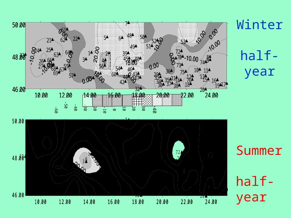
Winter half-year

+

40

+30

+20

+10

0

-10

-20

-30

-40

-50

-60

10.00 12.00 14.00 16.00 18.00 20.00 22.00 24.0046.00

48.00

50.00

1 23 4

5 6

7

89

10 1112 13

14 15 161718 19

20

21 22

2324 25

2627 28

29

3031

32

3334 35

36

37 38

394041

424344

45

46

47

48

49

50

5152 53

5455 56

57 5859

60

61

62

63 64

6566

676869

707172

73 74

7576

10.00 12.00 14.00 16.00 18.00 20.00 22.00 24.0046.00

48.00

50.00

10.00 12.00 14.00 16.00 18.00 20.00 22.00 24.0046.00

48.00

50.00

1 23 4

5 6

7

89

10 1112 13

14 15 161718 19

20

21 22

2324 25

2627 28

29

3031

32

3334 35

36

37 38

394041

42

4344

45

46

47

48

49

50

5152 53

5455 56

57 5859

60

61

62

63 64

6566

676869

707172

73 74

75

76

10.00 12.00 14.00 16.00 18.00 20.00 22.00 24.0046.00

48.00

50.00

Summer half-year

Example: Change field for Europe

0 20 40 E

60 S

50

40

Analysis of Regional Climate Change Scenarios for Hungary

MAGICC/SCENGENWigley et al., 2001;run & elaboration:Schlanger et al., 2003

CHANGES FROM SCENGENCHANGES FROM SCENGEN (7 - 16 models: inter-quartals)(7 - 16 models: inter-quartals)

Középhőmérséklet [°C] Napi hőingás [°C] Max. hőmérséklet [°C] Min. hőmérséklet [°C]

Felhőborítottság [%] Csapadékmennyiség [%] Légnyomás [hPa] Szélsebesség [%]

0

2

4

6

8

10

12

DJF

MA

M

JJA

SO

N

DJF

MA

M

JJA

SO

N

2050 2100

0

2

4

6

8

10

12

DJF

MA

M

JJA

SO

N

DJF

MA

M

JJA

SO

N

2050 2100

0

2

4

6

8

10

12

DJF

MA

M

JJA

SO

N

DJF

MA

M

JJA

SO

N

2050 2100

-3-2-1012345

DJF

MA

M

JJA

SO

N

DJF

MA

M

JJA

SO

N

2050 2100

-50-40-30-20-10

0102030

DJF

MA

M

JJA

SO

N

DJF

MA

M

JJA

SO

N

2050 2100

-80

-60

-40

-20

0

20

40

60

DJF

MA

M

JJA

SO

N

DJF

MA

M

JJA

SO

N2050 2100

-3-2-1012345

DJF

MA

M

JJA

SO

N

DJF

MA

M

JJA

SO

N

2050 2100

-20

-10

0

10

20

30

DJF

MA

M

JJA

SO

N

DJF

MA

M

JJA

SO

N

2050 2100

Mean temperature

K K K K

% % %hPa

Diurnal temp. range Max. temperature Min. temperature

Cloud coverage Precipitation amount Vapour pressure Wind speed

Data for cloudinessGround-based visual observationsGround-based visual observations

• 1973-1996 (24 years)• 172 observation srtations• EECRA data-base (Hahn & Warren,

1999)

GCM-output fields (clouds, etc.)

• 7-16 GCM modell adatai (CCC-EQ, CSIRO1, CSIRO2, ECHAM3, HAD-CM2, UKTR, UKHI-EQ for clouds)

• 2050 - B1 scenario (1,1 K warming) (MAGICC/SCENGEN diagnostics)

• 1961-1990 reference period (0 change)

• Output fields at 5 X 5 deg. rectangles

Distribution of the 172 stations in Eastern Europe

41,2542,5043,7545,0046,2547,5048,7550,0051,25

18,75 20,00 21,25 22,50 23,75 25,00 26,25 27,50 28,75 30,00 31,25

lat. N

Data for cloudiness (cont.)

Outgoing longwave radiation (OLR)

• 1979-2000 (22 years)

• 2,5 X 2,5 deg. resolution

• NOAA/NCEP TIROS-N quasi-polar satellites, AVHRR sensors

Main regulator of OLR: the cloud coverage - Correlation coefficients

(N = 18 : 1979-1996)

Orbital altitude: ~ 850 km

Original resolution: 1 - 3 kmFrequency of images: ~ 6

hours

NOAA

NOAA - NOAA - TIROSTIROS

  

   

 

1 2 3 4 5 6 7 8 9 10 11 12

N region -0,10 -0,43 -0,65 -0,73 -0,92 -0,55 -0,94 -0,94 -0,97 -0,85 -0,65 -0,54S region -0,79 -0,77 -0,80 -0,34 -0,91 -0,90 -0,93 -0,96 -0,93 -0,87 -0,79 -0,44

CHANGE OF CLOUDINESS IN EASTERN-EUROPEChange of cloud cover 7 GCMs (%/0.5 K)

-4,0

-3,0

-2,0

-1,0

0,0

1,0

1 2 3 4 5 6 7 8 9 10 11 12Months

%

Empirical change of OLR (%/0.5 K)

-20

-10

0

10

201 2 3 4 5 6 7 8 9 10 11 12

Months%

Empirical change of cloudiness (% /0.5 K)

-20-15-10

-505

1015

1 2 3 4 5 6 7 8 9 10 11 12Months

%

1973-19961973-1996r = 0.749r = 0.749d<T>/dt = 0.021 K/yrd<T>/dt = 0.021 K/yr

1979-20001979-2000r = 0.736r = 0.736d<T>/dt = 0.022 K/yrd<T>/dt = 0.022 K/yr

Index Winterhalf-year

0,5*dp/d<T>Summerhalf-year

0,5*dp/d<T>

Six points’ meanpressure (hPa)

1018, 9 1,82 1015,0 -0,13

45 N – 50 N grad.[hPa(10 fok)-1]

0,78 0,59 -1,17 -0,69

20 E – (10+30)/2E[hPa(10 fok)-1]

1,05 0,98 0,81 0,04

. . .

. ..

50 N

45 N

20 E10 E 30 E

www.cru.uea.ac.uk/cru/data/pressure.htm

Data: CRU - Norwich University,

VALIDATION OF PRECIPITATION VALIDATION OF PRECIPITATION TENDENCIES FOR 1999-2003 TENDENCIES FOR 1999-2003

Transsylvanean Basin

Areamean

Annualtotal

Winterhalf-year

Summerhalf-year

1999-2003 551,4 192,6 358,81974-1998 600,5 226,0 374,5Diff. in mm -49,1 -33,4 -15,7In % -8,2% -14,8% -4,2%

Area mean precipitation in the Transsylvanean Basin

0

10

20

30

40

50

60

70

80

90

100

1 2 3 4 5 6 7 8 9 10 11 12

1999-2003

25 yrs clim

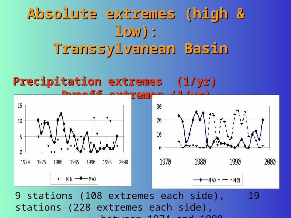
Absolute extremes (high & low):Absolute extremes (high & low): Transsylvanean BasinTranssylvanean Basin

Precipitation extremes (1/yr)Precipitation extremes (1/yr) Runoff extremes (1/yr) Runoff extremes (1/yr)

0

10

20

30

1970 1980 1990 2000

MAX MIN

0

5

10

15

1970 1975 1980 1985 1990 1995 2000

MIN MAX

9 stations (108 extremes each side), 19 stations (228 extremes each side), between 1974 and 1998

CONCLUSIONCONCLUSION100 m vertical difference corresponds to 35 mm increase of annual

precipitation, with a decrease from the oceans towards the inner continent.

The annual mean and the first three Fourier components explain 94 % of variance of the 25 years mean; but 66% of year-by-year anomalies.

Response of precipitation is not unequivocal along the upper-Danube region. Hungary is characterised by slightly negative changes in both half-years. To the East in the Carpathians, the signs are un-equivocally negative, to the west in the Alpines they are positive.

For an expected 0.5 K global warming the order of local changes is a few tens of percents of the total amount, in either direction.

Precipitation of the independent 1999-2003 period supports the extrapolation of the observed negative trends in the 1974-1998 warming period for the Transsylvanean basin.

CONCLUSION (contd.)CONCLUSION (contd.)These changes are qualitatively supported by independent empirical

and GCM-outputs, including precipitation and also cloudiness, however, the latter changes are rather diverse among the models, and somewhat smaller.

Changes of cloudiness and OLR qualitatively remind the decreasing precipitation in the observed (by now) Eastern European region.

Sea level pressure fields exhibit anticyclone–like relative modification in the central and eastern parts of the region, with precipitation decrease; whereas the observed precipitation increase in the Alpine region can not be directly related to the large scale sea-level pressure changes.

Tendencies of runoff extremes may differ from those of preci-pitation, as illustrated on example of Transsylvanean basin.

                                                                          

                

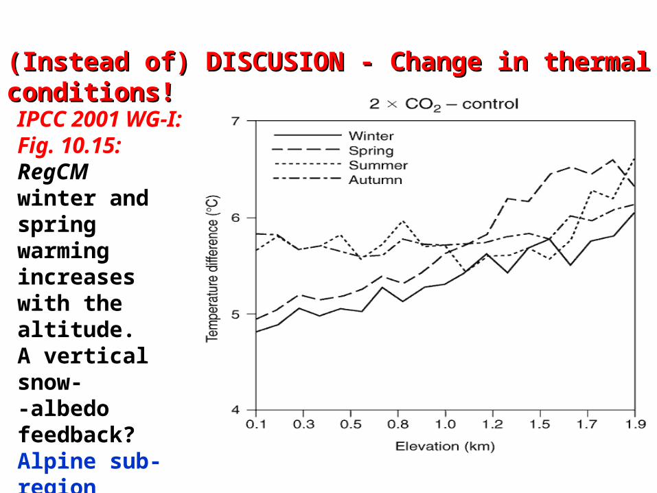
(Instead of) DISCUSION - Change in thermal conditions!(Instead of) DISCUSION - Change in thermal conditions!

IPCC 2001 WG-I:Fig. 10.15: RegCMwinter and spring warming increases with the altitude. A vertical snow--albedo feedback? Alpine sub-region(Giorgi et al. 1997)

ADDITION TO A REMARK ADDITION TO A REMARK IN VITUKI (DECEMBER 2003)IN VITUKI (DECEMBER 2003)

János MIKAJános MIKA

How effective the diurnal circulation How effective the diurnal circulation patterns patterns (by Péczely for Hungary) are? are?

CIRCULATIONAL AND PHYSICAL CIRCULATIONAL AND PHYSICAL FACTORS OF THE ANOMALIESFACTORS OF THE ANOMALIES

Any <A> local anomaly can be resolved (Mika, 1993) as:

M M

<A> = {qI}{AI}+ <q'I>{AI}+

I=1 I=1 M M

+{qI}<A'I>+ <q'I><A'I>

I=1 I=1

where the 1st term is zero.

<A> = C+P+M

C = <q'I>{AI} part of <A>

due to anomalous frequency distribution of circulation

types (circulation term),

P = {qI}<A'I> part of <A>

not directed by frequency of

circ. types (physical term),

M =<q'I> <A'

I> part of <A>

due to mixed influence.

-50%

0%

50%

100%

150%

Jan

Mar

May July

Sep

Nov

Precipitation: ++P M C

0%

50%

100%

Jan

Mar

May July

Sep

Nov

Precipitation: -- P M C

0%

50%

100%

Jan

Mar

May July

Sep

Nov

Temperature ++ P M C

-50%

0%

50%

100%

150%

Jan

Mar

May July

Sep

Nov

Temperature -- P M C

Correlation with the whole anomaly: PRECIPITATION

0

0.5

1

J an Mar May J uly Sep Nov

P

M

C

5%

0

0.5

1

1.5P

M

C

5%

Correlation with the whole anomaly: TEMPERATURE

Results from the 13 Péczely macrosynoptic types (Molnar J. et al., 2001):

Low portion of C term in * But fair correlation ofcase of macro-circulation. * C and full anomalies

MAXIMUM TEMPERATURE

-1,00

-0,50

0,00

0,50

1,001

4

6

8

12

16

24

MINIMUM TEMPERATURE

-1,00

-0,50

0,00

0,50

1,001

4

6

8

12

16

24

SUNSHINE DURATION

-1,00

-0,50

0,00

0,50

1,001

4

6

8

12

16

24

PRECIPITATION

-1,00

-0,50

0,00

0,50

1,001

4

6

8

12

16

24

Debrecen 1901-1996:Debrecen 1901-1996: Correlation Correlation of the clearlycirculation term with the monthly anomaly, averaged for 1, 4, 6, 8 years, and also for 12, 16 and 24 years..

burlesqueparody

frameboundary

conceptualtheoretical

SKIT, SCRIPT, OUTLINE, PLOT, ABSTRACT,

CAPSULATE, SYNOPSIS, SCREEN-PLAY, SKETCH

American synonyms

SCENARIOEnglish synonyms

TIME STORY LINE, THREAD

PLOT STORY UNFOLDING

machination

intriguetale

allegorydevelopmentmaturation