prague stochastics 2006 - mat.izt.uam.mxmat.izt.uam.mx/profs/anovikov/data/nov2006.pdfpreface prague...

PRAGUE STOCHASTICS 2006

Proceedings of the joint session of

7th Prague Symposium on Asymptotic Statistics

and

15th Prague Conference on Information Theory,Statistical Decision Functions and Random Processes,

held in Prague from August 21 to 25, 2006

Organised by

Charles UniversityFaculty of Mathematics and Physics

Department of Probability and Mathematical Statisticsand

Academy of Sciences of the Czech RepublicInstitute of Information Theory and Automation

Department of Stochastic Informatics

Edited by Marie Huskova and Martin Janzura

All rights reserved, no part of this publication may be reproduced or transmittedin any form or by any means, electronic, mechanical, photocopying or otherwise,without the prior written permission of the publisher.

c© (eds.) Marie Huskova and Martin Janzura, 2006c© MATFYZPRESS by publishing house of the Faculty of Mathematics and Physics,

Charles University in Prague, 2006

ISBN 80-86732-75-4

Preface

Prague Stochastics 2006, held in Prague from August 21 to 25, 2006, is an interna-tional scientific meeting that continues the tradition of organising Prague confer-ences on stochastics, established here five decades ago. The first Prague Conferenceon Information Theory, Statistical Decision Functions and Random Process was ini-tiated by Antonın Spacek in 1956. Prague Symposia on Asymptotic Statistics werefounded by Jaroslav Hajek in 1973. This year, we are commemorating the 80thanniversary of the birth date of this untimely deceased outstanding scientist.Traditionally, the scope of the proceedings, as well as the conference itself, is quiteextensive; the topics range from classical to very up-to date ones. It covers bothmethodological and applied statistics, theoretical and applied probability and, ofcourse, topics from information theory. We hope that all readers will find valuablecontributions and a number of papers of their interest in this rich spectrum ofscientific ideas.The printed part contains the plenary and invited papers, and the list of all contri-butions published in the volume. The CD disc, attached as an official part of thebook with the same ISBN code, contains all accepted papers.The editors would like to express their sincere thanks to the authors for their valu-able contributions, to the reviewers for prompt and careful reading of the papers,and to the organisers of the sections for the help with the entire reviewing process.Our thanks also go to our colleagues, in particular to Pavel Bocek and TomasHobza, for their technical editorial work. Without their devotion and diligence, theproceedings would never be completed.It is our pleasure to acknowledge that Prague Stochastics 2006 is held under theauspices of the Mayor of the City of Prague, the Bernoulli Society for MathematicalStatistics and Probability, and the Czech Statistical Society.

Prague, June 2006 Marie Huskova, Martin Janzura

Prague Stochastics 2006 I

Table of Contents

Plenary Lectures 1

Beran Rudolf:Multiple Affine Shrinkage 2

Stepan Josef:Measures with Given Marginals 14

Topsøe Flemming:Truth and Description 45

Invited Papers 55

Arjas Elja:Covariate information in complex event history data 56

Atkinson Anthony, Cerioli Andrea, Riani Marco:Clustering with the Forward Search 63

Aue Alexander, Horvath Lajos, Horvath Zsuzsanna:Level shifts and random walks 73

Drton Mathias:Algebraic Techniques for Gaussian Models 81

Dupacova Jitka:Contamination for multistage programs 91

Gordillo Luis F., Greenwood Priscilla, Kuske Rachel:Autonomous Stochastic Resonance 102

II Prague Stochastics 2006

Hanousek Jan, Kocenda Evzen, Svejnar Jan:Corporate Breakups and Performance 112

Inglot Tadeusz, Ledwina Teresa:Data Driven Tests for Regression 124

Kahle Waltraud:Incomplete Preventive Maintenance 138

Koenker Roger, Mizera Ivan:Alter egos of regularized maximum likelihood density estimators 145

Massam Helene:Conjugates for non decomposable graphs 158

Ondrejat Martin:Stochastic wave equations 165

Ruggeri Fabrizio, Sanso Bruno:Bayesian multi-fractal model of disk usage 173

Rukhin Andrew L.:Pattern Correlation Matrices 183

Saada Ellen:Hydrodynamics of attractive particle systems 193

Swart Jan M.:Duals and thinnings of contact process 203

van Lieshout M.N.M.:Campbell and Moment Measures for Finite Sequential Spatial Processes 215

Prague Stochastics 2006 III

Contributed Papers (CD ROM) 225

Aksin O. Zeynep, Cakan Nesrin, Karaesmen Fikri, Ormeci Lerzan:Joint Flexibility and Capacity Design 226

Astola Jaakko, Ryabko Boris:Universal Codes as a Basis for Time Series Testing 236

Benes Viktor, Helisova Katerina, Klebanov Lev:OUCP and SNCP 247

Bibi Abdelouahab, Gautier Antony:Minimum Distance Estimation 256

Brunel Elodie, Comte Fabienne:Adaptive estimation for censored regression 266

Cruz-Suarez Daniel, Montes-de-Oca Raul, Salem-Silva Francisco:Uniform Approximations of MDPs to Optimal Policies 278

Csiszar Imre, Matus Frantisek:GMLE for EF’s of infinite dimension 288

del Puerto Ines M., Molina Manuel, Ramos Alfonso:Bisexual branching model with immigration 298

Diop Aliou:Extremes of TARSV 308

Dostal Petr:Optimal trading strategies 318

Duffet Carole, Gannoun Ali, Guinot Christiane, Saracco Jerome:An affine equivariant estimator of conditional spatial median 327

IV Prague Stochastics 2006

Dyachkov Arkadii G.:Steganography Channel 334

Dzemyda Gintautas, Kurasova Olga:Visualization of Correlation-Based Data 344

Fabian Zdenek:Johnson characteristics 354

Gontis Vygintas, Kaulakys Bronislovas, Miglius Alaburda:Long-range stochastic point processes 364

Gordienko Evgueni, Novikov Andrey:Probability metrics and robustness 374

Harremoes Peter:Thinning 388

Hobza Tomas, Pardo Leandro:Robust median estimator 396

Hormann Siegfried:Augmented GARCH (1,1) 407

Houda Michal:Aproximations of stochastic and robust optimization programs 418

Houda Michal, Kankova Vlasta:Empirical Processes in Stochastic Programming 426

Huskova Marie, Koubkova Alena:Changes in autoregression 437

Prague Stochastics 2006 V

Iglesias-Perez M. del Carmen, Jacome M. Amalia:Presmoothed estimation with truncated and censored data 448

Kan Yuri:Quantile Comparison 458

Klaassen Chris A.J. , Mokveld Philip J., van Es Bert:Current duration versus length biased sampling 466

Kopa Milos, Post Thierry:FSD Efficiency Tests 475

Koubkova Alena:Sequential Change-Point Analysis 484

Lachout Petr:Sensitivity via infimum functional 495

Lao Wei, Stummer Wolfgang:Bayes risks for financial model choices 505

Laurincikas Antanas:On one application of the theory of processes in analytic number theory 515

Manstavicius Eugenijus:Probabilities in Combinatorics 523

Miyagawa Shigeyoshi, Morita Yoji, Rahman Md. Jahanur:Precautionary Demand by Financial Anxieties 533

Nagaev Sergey:On the best constants in the Burkholder type inequality 544

VI Prague Stochastics 2006

Novikov Andrey:Locally most powerful two-stage tests 554

Omelka Marek:Alternative CI for regression M-estimators 568

Pawlas Zbynek:Distribution function in germ-grain models 579

Pospısil Jan:On Ergodicity of Stochastic Evolution Equations 590

Rublık Frantisek:Principal Components 600

Siemenikhin Konstantin:On Linearity of Minimax Estimates 611

Simecek Petr:Classes of Gaussian, Discrete and Binary Representable Independence Models... 622

Sitar Milan, Sladky Karel:Optimality Conditions in Semi-Markov Decision Processes 633

Smıd Martin:Markov Properties of Limit Order Markets 644

Steland Ansgar:Monitoring LS Residuals 655

Streit Franz:Model Selection by Statistical Tests 666

Prague Stochastics 2006 VII

Stummer Wolfgang:Decisions about financial models 674

Takano Seiji:Inequality of Relative Entropy 680

Tishkovskaya Svetlana:Optimal Grouping in Bayesian Estimation 690

Vajda Igor, van der Meulen Edward C.:On Estimation and Testing by Means of φ-disparities 701

Vajda Igor, Zvarova Jana:Informations, Entropies and Bayesian Decisions 709

Vajda Istvan:Analysis of semi-log-optimal investment strategies 719

Vısek Jan Amos:Least Trimmed Squares - Sensitivity Study 728

Yurachkivsky Andriy :Random hypermeasures 739

Index of Authors A

Locally most powerful two-stage testsAndrey Novikov

Abstract: The problem of testing a simple hypothesis against a composite one-sided alternative is considered. The aim is to find a test which maximizes the slopeof the power function at the point of the null-hypothesis over all tests with fixedlevels of the first-kind error probability and of the average sample number under thenull-hypothesis. For the two-stage tests, the structure of the optimal decision ruleand the optimal continuation rule is given (the observations are not supposed tobe independent). Numerical results on the efficiency of the optimal two-stage tests,with respect to both the optimal fixed sample-size test and the optimal sequentialtest by R.Berk, are given.

MSC 2000: 62F03, 62F05, 62L10, 62M02, 62M07Key words: Statistical hypotheses testing, two-stage test, sequential test, regularexperiment, LAN, locally most powerful test, simple hypothesis, composite alter-native

1 Introduction

This work is motivated by recent results of the author ([8], [9]) on two-stage hy-potheses tests for two simple parametric hypotheses based on regular statisticalexperiments.

In that case, the optimal two-stage tests perform rather competitively withrespect to the optimal sequential tests known as sequential probability ratio tests(SPRT), due to A. Wald [11]. At the same time, the SPRT’s are known to beoptimal essentially for independent and identically distributed observations (see, forexample, [2]), while the two-stage tests have the advantage that they are applicableto any stochastic sequence of observations, and are relatively easy to evaluate (see[8], [9]). In some sense, they are simply ”two-step” versions of the well-knownNeyman-Pearson test (see, for example, [4]), and with essentially the same way ofproof (see [8]), so they are nearly as universal as the Neyman-Pearson test. The realproblem of their applicability is the lack of situations in which a simple hypothesisagainst a simple alternative is to be tested.

An approach to sequential testing a simple hypothesis against a composite al-ternative has been proposed by R. Berk in [1]. Again, due to [1], the optimal(called locally most powerful) sequential test exists in the case of independent and

Acknowledgement. The author wishes to thank the anonymous referee for his valuable sug-gestions on the improvement of the article.

Locally most powerful two-stage tests 555

identically distributed observations. There are no known results on optimality of se-quential hypotheses testing for more general stochastic sequences in the frameworkof this approach.

The main aim of this paper is to study the properties of two-stage tests of asimple hypothesis against a composite alternative in the framework of the approachof R. Berk. Because of particular simplicity of two-stage tests, we do not need someof the assumptions made in [1], in particular, we do not suppose the independenceof the observations at the two stages of the statistical experiment.

In Section 2, we study the structure of the optimal two-stage test in a rathergeneral context of statistical experiment. To deal with the derivative of the powerfunction we discuss some regularity conditions, which guarantee its existence.

In Section 3, we apply the results of Section 2 for optimal two-stage tests totesting hypotheses about the drift of a Wiener process with a lineal drift and givesome numerical results on the efficiency of the optimal two-stage tests with respectto both optimal one-stage tests, and to the locally most powerful sequential test ofR. Berk.

2 The structure of the optimal two-stage tests

In this section, we give a general framework for two-stage hypotheses tests, anddescribe the structure of the optimal two-stage test.

2.1 General framework. Definitions

Let us assume that we can observe in a statistical experiment a random variable X(the first stage of the experiment), and, depending on its value, either stop at thefirst stage or get to a second stage, obtaining an additional portion of observationsY . In any case we have to take a final decision about the distribution from which thevector (X,Y ) comes. This type of experiment can be thought of as an alternativeto fixed-size sampling, as in the Neyman-Pearson test, and to completely sequentialtests like the Wald’s sequential probability ratio test. For example, the usual fixedsample-size test is a particular case of this scheme, corresponding to never going tothe second stage, and making the inference on the base of the X-observation.

Let us assume that the vector (X,Y ) follows a parametric distribution with aprobability density function fθ(x, y) with respect to a product-measure µ1 ⊗ µ2 onthe space of values of (X,Y ), where θ ∈ Θ ⊂ R is some parameter. Thus, fθ(x) =∫fθ(x, y)dµ2(y) is the marginal density function of the first-stage component X

with respect to µ1.Let θ0 be such that there exists θ1, θ0 < θ1 6∞ for which [θ0, θ1) ⊂ Θ. In this

paper, we deal with testing the simple hypothesis H0 : θ = θ0 against the compositeone-sided alternative H1 : θ > θ0.

For a pair of hypotheses H0 and H1 let us define a (two-stage) test as a tripletof measurable functions (φ1(x), φ2(x, y), χ(x)), all of them taking values in [0, 1],

556 Prague Stochastics 2006

with the following interpretation:

• φ1(x) being the conditional probability, given a first-stage observation x, toreject H0,

• φ2(x, y) the conditional probability, given observations up to the second stage(x, y), to reject H0, and

• χ(x) being the conditional probability, given the first-stage observation x, toget to the second stage (to continue sampling).

The functions φ1(x), φ2(x, y) can be considered as (randomized) decision rulesat the respective stages of the experiment, and χ(x) as a (randomized) continuationrule. So, for example, the particular case χ(x) ≡ 0 corresponds to a ”fixed sample-size” test, with no observations at the second stage (in fact, in this case φ2(x, y)has to play no role, although formally we have to give some value to it, for exampleφ2(x, y) ≡ 0 or φ2(x, y) ≡ 1, or whatever. In what follows we will see that it doesnot have any importance for the performance of the test).

As usual in the context of hypotheses testing we define the power function asthe (total) probability to reject H0 when the true parameter of the distribution of(X,Y ) is θ:

P (θ) = Eθ [φ1(X)(1− χ(X)) + φ2(X,Y )χ(X)] . (1)

As in [1], we are interested in maximizing P ′(θ0) and minimizing P (θ0) (calledthe error probability of the first kind). Also, we have to take into account the costof additional observations, if any. As the first stage is always present, the onlyvariable part is naturally related to

C(θ) = Eθχ(X), (2)

the probability of continuing observations up to the second stage, given θ. As in[1], we will only pay attention to the value of C(θ) under H0, i.e. C(θ0).

2.2 Differentiability of the power function

To deal with the derivative of the power function (1), we have to be sure that itexists. In [1], there are conditions ensuring the differentiability of P (θ) for theexperiment consisting in observing sequentially independent and identically dis-tributed random variables X1, X2, . . . , Xn, . . . and any stopping time τ based onit, for which Eθτ < ∞. In our case, in view of (1) the conditions for existenceof the derivative might be very mild. A very natural candidate for this is somedifferentiability condition of the family {fθ(x, y)}θ∈Θ at θ = θ0. Essentially, weneed the possibility to calculate the derivative of the power function (1) at θ = θ0differentiating under the integral sign.

So, we will suppose that at θ = θ0 the following condition holds.


C1. The power function P (θ) (1) of any two-stage test is differentiable and thereexists a µ1 ⊗ µ2-integrable function ψθ(x, y) such that

P ′(θ) =∫ψθ(x, y) [φ1(x)(1− χ(x)) + φ2(x, y)χ(x)] dµ1 ⊗ µ2(x, y)

Typically, one would expect that ψθ(x, y) = f ′θ(x, y) = ∂fθ∂θ (x, y) if this derivative

exists. If it does not, but C1 still holds, we will keep using this notation, i.e.

f ′θ(x, y) ≡ ψθ(x, y) (3)

by definition.There are different ways to guarantee C1. A very closely related discussion can

be found in [5], where some references to earlier papers are given.In particular, it is easy to see that condition C1 is satisfied if fθ(x, y) is L1-

differentiable in the following sense (cf., e.g., [5]).C2. There exists a function ψθ(x, y) such that

∫|ψθ(x, y)|dµ1 ⊗ µ2(x, y) < ∞

and ∫|fθ+u(x, y)− fθ(x, y)− ψθ(x, y)u|dµ1 ⊗ µ2(x, y) = o(u),

as u→ 0.In a rather standard way, in turn, this condition holds if

√fθ(x, y) is L2-

differentiable in the following sense (see, for example, [3]).C3. There exists a function ψθ(x, y) such that

∫ψ2θ(x, y)dµ1⊗µ2(x, y) <∞ and∫

(√fθ+u(x, y)−

√fθ(x, y)− ψθ(x, y)u)2dµ1 ⊗ µ2(x, y) = o(u2),

as u→ 0.Although C2 seems to be more natural in the context of hypotheses testing,

C3 may be preferable dealing with regular statistical experiments and/or locallyasymptotically normal (LAN) experiments (see, for example, [3]).

In what follows, we will only use condition C1, seemingly close to the weakestpossible one.

Note that in all conditions C1-C3 we need in effect only the right-differentiabilityat θ = θ0 due to the essence of our testing problem.

Concluding this section let us note that condition C1 implies that for any one-stage test φ1(x) (with χ(x) ≡ 0) by Fubini’s theorem

P ′(θ) =∫φ1(x)

[∫ψθ(x, y)dµ2(y)

]dµ1(x),

justifying the notation

f ′θ(x) ≡∫ψθ(x, y)dµ2(y). (4)


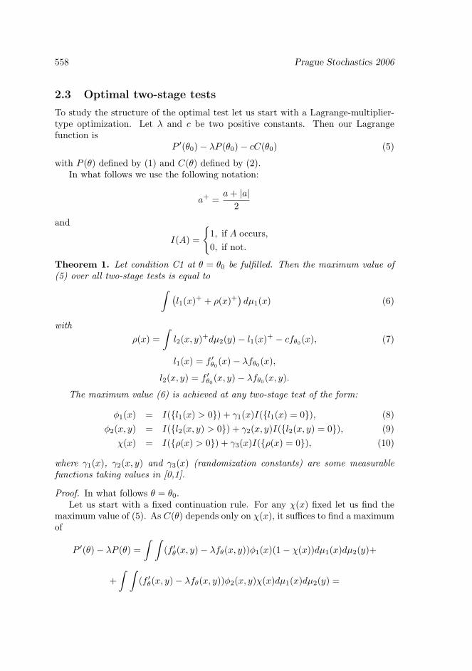
2.3 Optimal two-stage tests

To study the structure of the optimal test let us start with a Lagrange-multiplier-type optimization. Let λ and c be two positive constants. Then our Lagrangefunction is

P ′(θ0)− λP (θ0)− cC(θ0) (5)

with P (θ) defined by (1) and C(θ) defined by (2).In what follows we use the following notation:

a+ =a+ |a|

2

and

I(A) =

{1, if A occurs,0, if not.

Theorem 1. Let condition C1 at θ = θ0 be fulfilled. Then the maximum value of(5) over all two-stage tests is equal to∫ (

l1(x)+ + ρ(x)+)dµ1(x) (6)

withρ(x) =

∫l2(x, y)+dµ2(y)− l1(x)+ − cfθ0(x), (7)

l1(x) = f ′θ0(x)− λfθ0(x),

l2(x, y) = f ′θ0(x, y)− λfθ0(x, y).

The maximum value (6) is achieved at any two-stage test of the form:

φ1(x) = I({l1(x) > 0}) + γ1(x)I({l1(x) = 0}), (8)φ2(x, y) = I({l2(x, y) > 0}) + γ2(x, y)I({l2(x, y) = 0}), (9)

χ(x) = I({ρ(x) > 0}) + γ3(x)I({ρ(x) = 0}), (10)

where γ1(x), γ2(x, y) and γ3(x) (randomization constants) are some measurablefunctions taking values in [0,1].

Proof. In what follows θ = θ0.Let us start with a fixed continuation rule. For any χ(x) fixed let us find the

maximum value of (5). As C(θ) depends only on χ(x), it suffices to find a maximumof

P ′(θ)− λP (θ) =∫ ∫

(f ′θ(x, y)− λfθ(x, y))φ1(x)(1− χ(x))dµ1(x)dµ2(y)+

+∫ ∫

(f ′θ(x, y)− λfθ(x, y))φ2(x, y)χ(x)dµ1(x)dµ2(y) =


=∫

(f ′θ(x)− λfθ(x))φ1(x)(1− χ(x))dµ1(x)+

+∫ ∫

(f ′θ(x, y)− λfθ(x, y))φ2(x, y)χ(x)dµ1(x)dµ2(y), (11)

were we used condition C1 to calculate P ′(θ) and definitions (3) and (4).The first summand on the right-hand side of (11) does not exceed∫

(f ′θ(x)− λfθ(x))+(1− χ(x))dµ1(x),

because their difference is equal to∫(f ′θ(x)− λfθ(x))(I({f ′θ(x)− λfθ(x) > 0})− φ1(x))(1− χ(x))dµ1(x), (12)

which is non-negative due to

(f ′θ(x)− λfθ(x))(I({f ′θ(x)− λfθ(x) > 0})− φ1(x)) > 0,

because 0 6 φ1(x) 6 1.At the same time we see that the difference (12) is equal to 0 if φ1(x) has the

form (8).In the same way we see that the second summand on the right-hand side of (11)

does not exceed ∫ ∫(f ′θ(x, y)− λfθ(x, y))+χ(x)dµ1(x)dµ2(y),

and, again, this maximum is achieved if φ2(x, y) has the form (9).Now we have that for any χ(x)

P ′(θ)− λP (θ)− cC(θ) 6∫(f ′θ(x)−λfθ(x))+(1−χ(x))dµ1(x)+

∫ ∫(f ′θ(x, y)−λfθ(x, y))+χ(x)dµ1(x)dµ2(y)

−c∫χ(x)fθ(x)dµ1(x)

=∫

(f ′θ(x)− λfθ(x))+dµ1(x)

+∫ (∫

(f ′θ(x, y)− λfθ(x, y))+dµ2(y)− (f ′θ(x)− λfθ(x))+ − cfθ(x))χ(x)dµ1(x)

=∫l1(x)+dµ1(x) +

∫ρ(x)χ(x)dµ1(x). (13)


In the same way as above we see that the second term on the right-hand side of(13) does not exceed ∫

ρ(x)+dµ1(x), (14)

and that it coincides with (14) if χ(x) has the form (10).From this fact and (13) we conclude that

P ′(θ)−λP (θ)−cC(θ) 6∫l1(x)+dµ1(x)+

∫ρ(x)+dµ1(x) =

∫(l1(x)++ρ(x)+)dµ1(x),

with the equality if the test has the form (8)-(10).

Note. From the proof it is obvious that, more generally, to reach the maximumvalue (6) the relations (8)–(10) may be satisfied almost everywhere.

More than that, it is not difficult to see that if the maximum (6) is reached,then

φ1(x)(1− χ(x)) = (I({l1(x) > 0}) + γ1(x)I({l1(x) = 0})) (1− χ(x)),

φ2(x, y)χ(x) = (I({l2(x, y) > 0}) + γ2(x, y)I({l2(x, y) = 0}))χ(x),

χ(x) = I({ρ(x) > 0}) + γ3(x)I({ρ(x) = 0}),

almost everywhere, so this is the necessary and sufficient condition for reaching themaximum value (6).

2.4 Locally most powerful two-stage tests

Let us show now how the result of the preceding section can be applied to findinglocally most powerful two-stage tests.

Suppose first that we observe, in two stages, a discrete-time stochastic processX1, X2, . . . , Xn, . . . . In terms of the preceding section we have: X = (X1, X2, . . . ,Xn1) and Y = (Xn1+1, Xn2+2, . . . , Xn1+n2), where n1 (n2) is the number of obser-vations taken at the first (second) stage of the experiment.

Obviously, for any n1 and n2 fixed, Theorem 1 gives us the form of the optimaltest, which maximizes

P ′(θ0)− λP (θ0)− cN(θ0) (15)

over all tests with n1 observations at the first and n2 at the second stage of theexperiment, where N(θ) = n1 + n2C(θ) is the average sample number.

Let us denote by ∆ the class of all two-stage tests of the form (8)–(10) withx = (x1, x2, . . . , xn1) and y = (xn1+1, xn1+2, . . . , xn1+n2), corresponding to anycombination of n1 > 1, n2 > 1, λ > 0 and c > 0.

By Theorem 1, for any fixed λ > 0 and c > 0 any two-stage test has itscorresponding test in ∆ with a greater (or equal) value of the Lagrange function(15).

Let us start with the locally most powerful two-stage tests now.


From now on, for a two-stage test φ =< φ1, φ2, χ > let us use P (θ;φ) andN(θ;φ) for its power function and average sample number, respectively.

As in [1], we are interested in finding a test maximizing P ′(θ0;φ) over all two-stage tests φ with

P (θ0;φ) 6 α, (16)

andN(θ0;φ) 6 ν, (17)

where α ∈ (0, 1) and ν > 0 are some fixed numbers (locally most powerful test atθ = θ0).

LetL(φ;λ, c) = P ′(θ0;φ)− λP (θ0;φ)− cN(θ0;φ) . (18)

Let us suppose now that for some λ > 0 and c > 0 there is a test φ∗ ∈ ∆ suchthat

supφ∈∆

L(φ;λ, c) = L(φ∗;λ, c), (19)

and let α = P (θ0;φ∗) and ν = N(θ0;φ∗).It is easy to see that in this case φ∗ is the locally most powerful test among all

two-stage tests satisfying (16) and (17).Indeed, if φ is any such test, then

L(φ;λ, c) 6 L(φ∗;λ, c)

= P ′(θ0;φ∗)− λP (θ0;φ∗)− cN(θ0;φ∗) = P ′(θ0;φ∗)− λα− cν (20)

because of Theorem 1 and (19).On the other hand, because of (16) and (17),

L(φ;λ, c) = P ′(θ0;φ)− λP (θ0;φ)− cN(θ0;φ) > P ′(θ0;φ)− λα− cν, (21)

Combining (20) and (21) we have

P ′(θ0;φ) 6 P ′(θ0;φ∗),

which proves that φ∗ is locally most powerful.It is quite obvious that in the same way we can apply the result of the preceding

section for construction of the locally most powerful two-stage test for a continuous-time stochastic process.

In this case, the observations will be taken from a stochastic process X(t), t >0, and, in terms of the preceding section, the observations X and Y at the twostages, of the respective duration t1 and t2, can be taken as X(t1) and X(t1 + t2),respectively.

Again, by Theorem 1, the optimal two-stage test has the form (8)–(10) withx = x(t1) and y = x(t1 + t2), where x(t1) and x(t1 + t2) are the observed values of


X(t1) and X(t1 + t2), respectively, and fθ(x, y) corresponds to the two-dimensionaldistribution of (X(t1), X(t1 + t2)). Because of this, all the elements of the optimaltwo-stage test (8)–(10) are relatively easy to calculate, nearly as easy as in the caseof the discrete-time stochastic process above.

Acting in the same way as above in this section (see (19) and what follows), wecan find the locally most powerful two-stage test in this case as well.

It is worth mentioning that, generally speaking, there is no guarantee that thisway we can find the locally most powerful two-stage test for any given α and/orν (and even for some of them), but neither is it there in the case of [1], even forindependent and identically distributed observations.

As a promising fact let us note that in any case the optimization problem (19)is essentially numerical (two-dimensional optimization), so there is a hope that, inany concrete case, it can be solved with more or less difficulty, at least numerically.

3 Example: A Wiener process with a lineal drift

In this section, we apply the results of the preceding section to the case of testinghypotheses about the drift of a Wiener process with a lineal drift.

We observe the process ξ(t) = W (t) + θt, where W (t) is a standard Wienerprocess. At the first stage, we observe ξ(t) up to the time t1, then, if necessary, atthe second stage we observe ξ(t) for t2 time units more.

We are interested in testing H0 : θ = θ0 = 0 vs H1 : θ > 0 using a two-stagetest.

Because (ξ(t1), ξ(t1 + t2)) is a sufficient statistics, we can restrict our attentionto the distribution of the vector (X,Y ), where X = ξ(t1) and Y = ξ(t1 +t2)−ξ(t1).So, in the terms of the preceding section

fθ(x) = f1θ (x) =

1√t1φ

(x− θt1√

t1

), fθ(x, y) = f1

θ (x)f2θ (y),

f2θ (y) =

1√t2φ

(x− θt2√

t2

),

φ(x) being the probability distribution function of the standard normal distribution.In this case (θ0 = 0) it is not difficult to calculate:

f ′θ0(x) = xfθ0(x)

f ′θ0(x, y) = (x+ y)fθ0(x, y)

ρ(x) = (Eθ0(x+ Y − λ)+ − (x− λ)+ − ct2)fθ0(x)

= (√t2φ((x− λ)/

√t2)− |x− λ|Φ(−|x− λ|/

√t2)− ct2)fθ0(x),

where Φ(x) is the standard normal distribution function.


To define the optimal continuation rule (see Theorem 1) let us note that ρ(x) > 0is equivalent to φ(u)−|u|Φ(−|u|) > c

√t2, where u = (x−λ)/

√t2. Thus, the optimal

continuation rule isχ(x) = I({|x− λ|/

√t2 < a}),

where a = a(c√t2) is the positive solution of the equation

φ(u)− |u|Φ(−|u|) = c√t2.

Jointly with φ1(x) = I({x > λ}) and φ2(x) = I({x + y > λ}) this gives acomplete description of the optimal test (8)-(10) for any fixed t1 and t2.

Let us denote G(u) = φ(u) − |u|Φ(−|u|) for u ∈ R. Then for any λ > 0 andc > 0 and t1 > 0, t2 > 0 fixed the value (18) for the above test is equal to

√t1

(G

(λ√t1

)− c

√t1

)+√t2Eθ0

(G

(ξ(t1)− λ√

t2

)− c

√t2

)+

(22)

To find the locally most powerful test following the plan of Section 2.4, we needto find the supremum of (22) over all t1 > 0 and t2 > 0 (see (19)) for any λ > 0and c > 0 fixed.

Surprisingly, for some λ > 0 and c > 0 the maximum value of (22) is equal to 0and is achieved at t1 = t2 = 0, so the procedure of Section 2.4 fails. The worst ofall is that this happens for large values of λ which are necessary to hold the errorprobability (16) at a reasonably low level of α. Our numerical estimations showthat for α ≈ 0.1 or less the maximum value of (22) over all t1 > 0 and t2 > 0 is0. Nevertheless, for greater values of α the direct maximization of (22) gives usa definite level-α two-stage test, which turns out to be the locally most powerfullevel-α two-stage test, by the results of Section 2.4. Some numerical results forlarger α we show below in this Section.

To treat lower levels of α in this example we propose another plan.The idea is to start with a fixed t1 > 0 in maximization of (22), say, t1 = 1. It

is easy to see that the maximum of (22) with t1 = 1 over t2 > 0 is achieved at somet2 = r2. Starting from the pair (1, r2) it is not difficult to construct the two-stagetest giving the maximum to (22) (over t2 > 0) for any fixed t1.

Let us denote by P1(θ;λ, c) the power function of the two-stage test based ont1 = 1 and t2 = r2 giving the maximum (over t2) to (22) with t1 = 1, and letP ′1(θ0;λ, c) be its derivative at θ = θ0. Let, finally, be N1(θ0;λ, c) its averagesample number.

For t1 6= 1 we use, respectively, Pt1(θ;λ, c), P ′t1(θ0;λ, c) and Nt1(θ0;λ, c) for thecorresponding characteristics of the test giving the maximum (over t2) to (22) whent1 is held fixed.

It is not difficult to see that

Pt1(θ0;λ, c) = P1(θ0;λ√t1, c√t1), (23)


P ′t1(θ0;λ, c) =√t1P

′1(θ0;

λ√t1, c√t1), (24)

Nt1(θ0;λ, c) = t1N1(θ0;λ√t1, c√t1). (25)

If nowPt1(θ0;λ, c) ≈ α (26)

andNt1(θ0;λ, c) ≈ ν, (27)

from (23) and (25) we have that

P1(θ0;λ√t1, c√t1) ≈ α (28)

andt1 ≈ ν/N1(θ0;

λ√t1, c√t1),

and, by virtue of (24),

P ′t1(θ0;λ, c) ≈√νP ′1(θ0; λ√

t1, c√t1)√

N1(θ0; λ√t1, c√t1)

. (29)

Thus, to maximize the left-hand side of (29) over all tests subject to (26) and(27), it suffices to maximize the right-hand side of (29) subject to (28).

So, our candidate for the locally most powerful two-stage test is the test givingthe maximum to

P ′1(θ0;λ, c)√N1(θ0;λ, c)

(30)

subject toP1(θ0;λ, c) = α. (31)

The value of (30) is natural to interpret as the efficiency of the two-stage test,representing the ”specific slope”, per square root of the average sample numberunit. Because of that, let us denote its maximum value by E2 = E2(α) (here 2stands for ”two-stage”). Some numerical results on the evaluation of E2 can befound below.

It is very interesting to calculate the relative efficiency of the optimal two-stagetests with respect to the fixed sample-size test, and to the optimal sequential test.

Let us start with the ”fixed sample-size” tests.In terms of Section 2.1 it is a ”one-stage” test with no continuation region

(χ(x) ≡ 0). In the context of this example, this means that it is defined by a fixedtime t1 of the observation at the first stage, with no continuation.


Because the form of the decision rule is fixed by Theorem 1, we have as theoptimal one-stage test φ1(x) = I({x > λ}) with x = ξ(t1). Obviously, the powerfunction of such a test is P (θ0) = Pθ0(ξ(t1) > λ) = 1 − Φ(λ/

√t1) and P ′(θ0) =

Eθ0ξ(t1)I({ξ(t1) > λ}) =√t1 exp{−λ2/(2t1)}/

√2π with N(θ) = t1.

Defining λ in such a way that P (θ0) = α we have:

λ =√t1Φ−1(1− α),

where Φ−1(1− α) it the (1− α)-quantile of the standard normal distribution, andhence for the efficiency E1 = E1(α):

E1 = φ(Φ−1(1− α)). (32)

Again, 1 in E1 stands for ”one-stage”.

Now, let us evaluate the efficiency of the optimal sequential test. Formally, thecase of continuous-time stochastic processes is not covered in [1], so we make use ofthe results of [10] extending the locally most powerful tests of R. Berk to processeswith stationary independent increments. Because, as stated in [10], for exponentialfamilies the locally most powerful sequential test is a Wald’s SPRT for a pair ofconjugate values of θ, for which θ0 is an ”exceptional point”, we see that for thecase we are considering the optimal sequential test is an SPRT for two symmetricalvalues of θ. Being so, it is easy to calculate the characteristics of the test under H0,because in this case the SPRT is defined by two constants −A < 0 and B > 0 andstops when ξ(t) for the first time hits any one of the two boundaries, that is, itsstopping time is τ = sup{t : −A < ξ(t) < B}. Because under H0 there is no drift(ξ(t) ≡ W (t)), all the characteristics are easy to calculate using the well-knownformulas for the ruin probability. This way, we come to the efficiency E∞ of theoptimal sequential test:

E∞ =√α(1− α).

Obviously, it should be E1 < E2 < E∞. In the table below we give the values ofE1, E2 and E∞ for some usual (or interesting) values of α. For convenience, we alsoshow their relative values RE2 = E2/E1 and RE∞ = E∞/E2 to make visible theincrease in the specific slope from using ”respectively more” stages of the experi-ment. It should be noted that the increase E2/E1 is really due to one additionalstage of the experiment, while E∞/E2 corresponds to going to an ”infinitely much”richer experiment, with a continuum of ”stages” in place of two stages as in E2.


α E1 E2 E∞ RE2 RE∞

50% 0.39894 0.43484 0.50000 1.090 1.150

20% 0.28067 0.32867 0.40063 1.171 1.219

10% 0.17550 0.23374 0.30000 1.332 1.283

5.0% 0.10313 0.16143 0.21794 1.565 1.350

2.5% 0.05844 0.11054 0.15612 1.891 1.412

1.0% 0.02665 0.06733 0.09950 2.526 1.478

0.5% 0.01446 0.04630 0.07053 3.202 1.523

We note that the two-stage hypotheses tests are good competitors to the fullysequential tests. Taking into account that they do not require the independence ofthe observations, and thus are more applicable, they are a good prospect to studyin more details.

Examples of the two-stage tests for dependent observations will be given some-where else. The example we consider here deals with independent observations fortwo reasons. We need this case as a ”reference point” for efficiency evaluation,because there are no known optimality results of purely sequential tests for reason-ably general model with dependent observations, and, consequently, the efficiencycomparison of the two-stage tests with purely sequential tests would not be feasi-ble. Now, we can state that two-stage perform well even in the case of independentobservations. The second reason is that the model considered here serve as the”limiting” case for a rather broad class of locally asymptotically normal (LAN)experiments. In particular, we can mention, besides the well-known LAN experi-ments with independent identically distributed observations (see, e.g., [3]), regulardiscrete-time Markov ergodic stochastic processes (see [6], cf. also [7]). We ex-pect that the optimality results for the Wiener process will have consequences inasymptotic optimality for a larger class of LAN experiments.

Other promising application of two-stage tests seems to be the problem of testinga simple hypothesis versus a two-sided alternative, in which case unbiased tests areneeded. As stated in [5] the form of the locally most powerful unbiased sequentialtest is difficult to find. At the same time, unbiased two-stage tests are easy to find,at least in the example we considered here. So the locally most powerful unbiasedtwo-stage tests are waiting for being studied.

References

[1] Berk R.H. Locally most powerful sequential tests. Ann. Statist. V.3, No. 2,373–381, 1975

[2] DeGroot M. H. Optimal statistical decisions. McGraw-Hill Book Co., NewYork-London-Sydney, 1970.


[3] Le Cam, L. Asymptotic methods in statistical decision theory. Springer Seriesin Statistics. Springer-Verlag, New York–Berlin, 1986.

[4] Lehmann E.L. Testing statistical hypotheses. John Wiley & Sons, Inc., NewYork; Chapman & Hall, Ltd., London, 1959.

[5] Muller-Funk U., Pukelsheim F., Witting H. Locally most powerful tests fortwo-sided hypotheses. Probability and statistical decision theory, Vol. A (BadTatzmannsdorf, 1983), 31–56, Reidel, Dordrecht, 1985.

[6] Novikov A. Uniform asymptotic expansion of likelihood ratio for Markovdependent observations. Ann. Inst. Statist. Math., V. 53, No. 4, 799–809,2001.

[7] Novikov A. Efficiency of sequential hypotheses testing. Aportacionesmatematicas. Serie Comunicaciones, 30:71–79, 2002.

[8] Novikov A. Optimality of two-stage hypothesis testsCOMPSTAT Proceedingsin Computational Statistics, 16th Symposium held in Prague, Czech Republic,Physica-Verlag, pp. 1601–1608, 2004.

[9] Novikov A. Asymptotic optimality of two-stage hypotheses tests. Aporta-ciones Matematicas. Serie Comunicaciones, 35:37–43, 2005.

[10] Roters M. Locally most powerful sequential tests for processes of the exponen-tial class with stationary and independent increments. Metrika, 39, no. 3-4,177–183, 1992.

[11] Wald A. Sequential analysis. John Wiley & Sons, Inc., New York; Chapman& Hall, Ltd., London, 1947

Andrey Novikov: UAM-Iztapalapa, Depto. Matematicas, San Rafael Atlixco #186,col. Vicentina, Mexico, 09340, Mexico, [email protected]

prague stochastics 2006 - mat.izt.uam.mxmat.izt.uam.mx/profs/anovikov/data/nov2006.pdfpreface prague...

Documents