prague stochastics 2006 - universidad …mat.izt.uam.mx/profs/anovikov/data/gordnov2006.pdf ·...
TRANSCRIPT

PRAGUE STOCHASTICS 2006
Proceedings of the joint session of
7th Prague Symposium on Asymptotic Statistics
and
15th Prague Conference on Information Theory,Statistical Decision Functions and Random Processes,
held in Prague from August 21 to 25, 2006
Organised by
Charles UniversityFaculty of Mathematics and Physics
Department of Probability and Mathematical Statisticsand
Academy of Sciences of the Czech RepublicInstitute of Information Theory and Automation
Department of Stochastic Informatics
Edited by Marie Huskova and Martin Janzura

All rights reserved, no part of this publication may be reproduced or transmittedin any form or by any means, electronic, mechanical, photocopying or otherwise,without the prior written permission of the publisher.
c© (eds.) Marie Huskova and Martin Janzura, 2006c© MATFYZPRESS by publishing house of the Faculty of Mathematics and Physics,
Charles University in Prague, 2006
ISBN 80-86732-75-4

Preface
Prague Stochastics 2006, held in Prague from August 21 to 25, 2006, is an interna-tional scientific meeting that continues the tradition of organising Prague confer-ences on stochastics, established here five decades ago. The first Prague Conferenceon Information Theory, Statistical Decision Functions and Random Process was ini-tiated by Antonın Spacek in 1956. Prague Symposia on Asymptotic Statistics werefounded by Jaroslav Hajek in 1973. This year, we are commemorating the 80thanniversary of the birth date of this untimely deceased outstanding scientist.Traditionally, the scope of the proceedings, as well as the conference itself, is quiteextensive; the topics range from classical to very up-to date ones. It covers bothmethodological and applied statistics, theoretical and applied probability and, ofcourse, topics from information theory. We hope that all readers will find valuablecontributions and a number of papers of their interest in this rich spectrum ofscientific ideas.The printed part contains the plenary and invited papers, and the list of all contri-butions published in the volume. The CD disc, attached as an official part of thebook with the same ISBN code, contains all accepted papers.The editors would like to express their sincere thanks to the authors for their valu-able contributions, to the reviewers for prompt and careful reading of the papers,and to the organisers of the sections for the help with the entire reviewing process.Our thanks also go to our colleagues, in particular to Pavel Bocek and TomasHobza, for their technical editorial work. Without their devotion and diligence, theproceedings would never be completed.It is our pleasure to acknowledge that Prague Stochastics 2006 is held under theauspices of the Mayor of the City of Prague, the Bernoulli Society for MathematicalStatistics and Probability, and the Czech Statistical Society.
Prague, June 2006 Marie Huskova, Martin Janzura


Prague Stochastics 2006 I
Table of Contents
Plenary Lectures 1
Beran Rudolf:Multiple Affine Shrinkage 2
Stepan Josef:Measures with Given Marginals 14
Topsøe Flemming:Truth and Description 45
Invited Papers 55
Arjas Elja:Covariate information in complex event history data 56
Atkinson Anthony, Cerioli Andrea, Riani Marco:Clustering with the Forward Search 63
Aue Alexander, Horvath Lajos, Horvath Zsuzsanna:Level shifts and random walks 73
Drton Mathias:Algebraic Techniques for Gaussian Models 81
Dupacova Jitka:Contamination for multistage programs 91
Gordillo Luis F., Greenwood Priscilla, Kuske Rachel:Autonomous Stochastic Resonance 102
II Prague Stochastics 2006
Hanousek Jan, Kocenda Evzen, Svejnar Jan:Corporate Breakups and Performance 112
Inglot Tadeusz, Ledwina Teresa:Data Driven Tests for Regression 124
Kahle Waltraud:Incomplete Preventive Maintenance 138
Koenker Roger, Mizera Ivan:Alter egos of regularized maximum likelihood density estimators 145
Massam Helene:Conjugates for non decomposable graphs 158
Ondrejat Martin:Stochastic wave equations 165
Ruggeri Fabrizio, Sanso Bruno:Bayesian multi-fractal model of disk usage 173
Rukhin Andrew L.:Pattern Correlation Matrices 183
Saada Ellen:Hydrodynamics of attractive particle systems 193
Swart Jan M.:Duals and thinnings of contact process 203
van Lieshout M.N.M.:Campbell and Moment Measures for Finite Sequential Spatial Processes 215
Prague Stochastics 2006 III
Contributed Papers (CD ROM) 225
Aksin O. Zeynep, Cakan Nesrin, Karaesmen Fikri, Ormeci Lerzan:Joint Flexibility and Capacity Design 226
Astola Jaakko, Ryabko Boris:Universal Codes as a Basis for Time Series Testing 236
Benes Viktor, Helisova Katerina, Klebanov Lev:OUCP and SNCP 247
Bibi Abdelouahab, Gautier Antony:Minimum Distance Estimation 256
Brunel Elodie, Comte Fabienne:Adaptive estimation for censored regression 266
Cruz-Suarez Daniel, Montes-de-Oca Raul, Salem-Silva Francisco:Uniform Approximations of MDPs to Optimal Policies 278
Csiszar Imre, Matus Frantisek:GMLE for EF’s of infinite dimension 288
del Puerto Ines M., Molina Manuel, Ramos Alfonso:Bisexual branching model with immigration 298
Diop Aliou:Extremes of TARSV 308
Dostal Petr:Optimal trading strategies 318
Duffet Carole, Gannoun Ali, Guinot Christiane, Saracco Jerome:An affine equivariant estimator of conditional spatial median 327

IV Prague Stochastics 2006
Dyachkov Arkadii G.:Steganography Channel 334
Dzemyda Gintautas, Kurasova Olga:Visualization of Correlation-Based Data 344
Fabian Zdenek:Johnson characteristics 354
Gontis Vygintas, Kaulakys Bronislovas, Miglius Alaburda:Long-range stochastic point processes 364
Gordienko Evgueni, Novikov Andrey:Probability metrics and robustness 374
Harremoes Peter:Thinning 388
Hobza Tomas, Pardo Leandro:Robust median estimator 396
Hormann Siegfried:Augmented GARCH (1,1) 407
Houda Michal:Aproximations of stochastic and robust optimization programs 418
Houda Michal, Kankova Vlasta:Empirical Processes in Stochastic Programming 426
Huskova Marie, Koubkova Alena:Changes in autoregression 437
Prague Stochastics 2006 V
Iglesias-Perez M. del Carmen, Jacome M. Amalia:Presmoothed estimation with truncated and censored data 448
Kan Yuri:Quantile Comparison 458
Klaassen Chris A.J. , Mokveld Philip J., van Es Bert:Current duration versus length biased sampling 466
Kopa Milos, Post Thierry:FSD Efficiency Tests 475
Koubkova Alena:Sequential Change-Point Analysis 484
Lachout Petr:Sensitivity via infimum functional 495
Lao Wei, Stummer Wolfgang:Bayes risks for financial model choices 505
Laurincikas Antanas:On one application of the theory of processes in analytic number theory 515
Manstavicius Eugenijus:Probabilities in Combinatorics 523
Miyagawa Shigeyoshi, Morita Yoji, Rahman Md. Jahanur:Precautionary Demand by Financial Anxieties 533
Nagaev Sergey:On the best constants in the Burkholder type inequality 544
VI Prague Stochastics 2006
Novikov Andrey:Locally most powerful two-stage tests 554
Omelka Marek:Alternative CI for regression M-estimators 568
Pawlas Zbynek:Distribution function in germ-grain models 579
Pospısil Jan:On Ergodicity of Stochastic Evolution Equations 590
Rublık Frantisek:Principal Components 600
Siemenikhin Konstantin:On Linearity of Minimax Estimates 611
Simecek Petr:Classes of Gaussian, Discrete and Binary Representable Independence Models... 622
Sitar Milan, Sladky Karel:Optimality Conditions in Semi-Markov Decision Processes 633
Smıd Martin:Markov Properties of Limit Order Markets 644
Steland Ansgar:Monitoring LS Residuals 655
Streit Franz:Model Selection by Statistical Tests 666

Prague Stochastics 2006 VII
Stummer Wolfgang:Decisions about financial models 674
Takano Seiji:Inequality of Relative Entropy 680
Tishkovskaya Svetlana:Optimal Grouping in Bayesian Estimation 690
Vajda Igor, van der Meulen Edward C.:On Estimation and Testing by Means of φ-disparities 701
Vajda Igor, Zvarova Jana:Informations, Entropies and Bayesian Decisions 709
Vajda Istvan:Analysis of semi-log-optimal investment strategies 719
Vısek Jan Amos:Least Trimmed Squares - Sensitivity Study 728
Yurachkivsky Andriy :Random hypermeasures 739
Index of Authors A

Probability metrics and robustness:Is the sample median more robust than the samplemean?Evgueni Gordienko, Andrey Novikov
Abstract: In this paper, we consider a modified concept of qualitative robustnessintroduced by Hampel (see [5]). The modification takes into account the asymp-totic normality of the estimators and allows to obtain quantitative estimates ofthe robustness in terms of suitable probability metrics. To this end, we measuredeviations from the model distribution by metrics rather than by the level of ”con-tamination” with a heavy-tail distribution.
We show that the ”robustness” of the sample mean and the sample medianstatistics depends on the choice of the metrics. In particular, we obtain a quanti-tative estimate of the ”robustness” of the sample mean, which is new in the caseof models with non-Gaussian distributions.
MSC 2000: 62F35, 60E15Key words: probability metric, sample mean, sample median, robust estimation
1 Introduction
In the paper of Hampel [5] the concept of qualitative robustness was introduced(see the definition in Section 3 below). According to his definition (which uses theProkhorov metric) the sample mean is not robust, but the sample median is ([5],and §2.2 in [6]).
In this paper, we define an alternative concept of robustness based on the Kan-torovich metric l (see Section 2). The use of the Kantorovich metric is justified byits closer relation to the mean absolute error of the estimators. To give a quanti-tative aspect to the robustness, we let it be related to some additional probabilitymetric µ, and call this (l − µ)-robustness.
The goal of the paper is to show that this type of robustness of estimatorscrucially depends on the choice of the metric µ. We give an example of probabilitymetric µ for which the sample mean is (l−µ)-robust but the sample median is not.The picture can turn over when using another metric (see Section 5).
The main result of the paper is the quantitative estimation of the (l − µ)-robustness of the sample mean when µ is the maximum of the Kantorovich metricand the Zolotarev metric ζ2 of order 2. More specifically, we show in Section 3 that
supn>1
√nl(Xn,
¯Xn) 6 cmax{l(F, F ), ζ2(F, F )}, (1)
Probability metrics and robustness 375
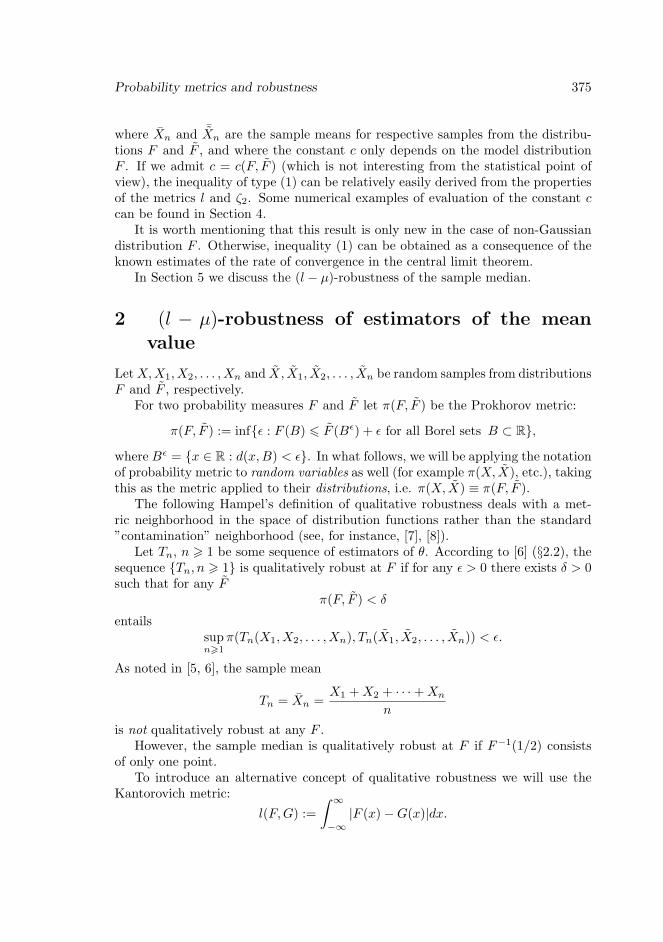
where Xn and ¯Xn are the sample means for respective samples from the distribu-tions F and F , and where the constant c only depends on the model distributionF . If we admit c = c(F, F ) (which is not interesting from the statistical point ofview), the inequality of type (1) can be relatively easily derived from the propertiesof the metrics l and ζ2. Some numerical examples of evaluation of the constant ccan be found in Section 4.
It is worth mentioning that this result is only new in the case of non-Gaussiandistribution F . Otherwise, inequality (1) can be obtained as a consequence of theknown estimates of the rate of convergence in the central limit theorem.
In Section 5 we discuss the (l − µ)-robustness of the sample median.
2 (l − µ)-robustness of estimators of the meanvalue
LetX,X1, X2, . . . , Xn and X, X1, X2, . . . , Xn be random samples from distributionsF and F , respectively.
For two probability measures F and F let π(F, F ) be the Prokhorov metric:
π(F, F ) := inf{ε : F (B) 6 F (Bε) + ε for all Borel sets B ⊂ R},
where Bε = {x ∈ R : d(x,B) < ε}. In what follows, we will be applying the notationof probability metric to random variables as well (for example π(X, X), etc.), takingthis as the metric applied to their distributions, i.e. π(X, X) ≡ π(F, F ).
The following Hampel’s definition of qualitative robustness deals with a met-ric neighborhood in the space of distribution functions rather than the standard”contamination” neighborhood (see, for instance, [7], [8]).
Let Tn, n > 1 be some sequence of estimators of θ. According to [6] (§2.2), thesequence {Tn, n > 1} is qualitatively robust at F if for any ε > 0 there exists δ > 0such that for any F
π(F, F ) < δ
entailssupn>1
π(Tn(X1, X2, . . . , Xn), Tn(X1, X2, . . . , Xn)) < ε.
As noted in [5, 6], the sample mean
Tn = Xn =X1 +X2 + · · ·+Xn
n
is not qualitatively robust at any F .However, the sample median is qualitatively robust at F if F−1(1/2) consists
of only one point.To introduce an alternative concept of qualitative robustness we will use the
Kantorovich metric:l(F,G) :=
∫ ∞
−∞|F (x)−G(x)|dx.
376 Prague Stochastics 2006
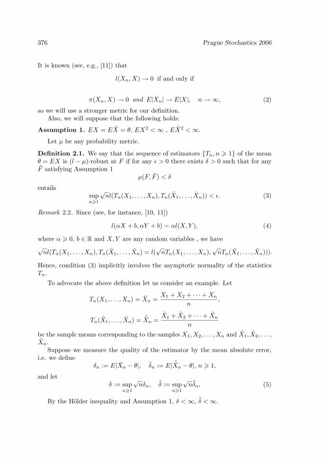
It is known (see, e.g., [11]) that
l(Xn, X) → 0 if and only if
π(Xn, X) → 0 and E|Xn| → E|X|, n→∞, (2)
so we will use a stronger metric for our definition.Also, we will suppose that the following holds:
Assumption 1. EX = EX = θ, EX2 <∞ , EX2 <∞.
Let µ be any probability metric.
Definition 2.1. We say that the sequence of estimators {Tn, n > 1} of the meanθ = EX is (l − µ)-robust at F if for any ε > 0 there exists δ > 0 such that for anyF satisfying Assumption 1
µ(F, F ) < δ
entailssupn>1
√nl(Tn(X1, . . . , Xn), Tn(X1, . . . , Xn)) < ε. (3)
Remark 2.2. Since (see, for instance, [10, 11])
l(αX + b, αY + b) = αl(X,Y ), (4)
where α > 0, b ∈ R and X,Y are any random variables , we have√nl(Tn(X1, . . . , Xn), Tn(X1, . . . , Xn) = l(
√nTn(X1, . . . , Xn),
√nTn(X1, . . . , Xn))).
Hence, condition (3) implicitly involves the asymptotic normality of the statisticsTn.
To advocate the above definition let us consider an example. Let
Tn(X1, . . . , Xn) = Xn =X1 +X2 + · · ·+Xn
n,
Tn(X1, . . . , Xn) = ¯Xn =X1 + X2 + · · ·+ Xn
n
be the sample means corresponding to the samples X1, X2, . . . , Xn and X1, X2, . . . ,Xn.
Suppose we measure the quality of the estimator by the mean absolute error,i.e. we define
δn := E|Xn − θ|, δn := E| ¯Xn − θ|, n > 1,
and letδ := sup
n>1
√nδn, δ := sup
n>1
√nδn, (5)
By the Holder inequality and Assumption 1, δ <∞, δ <∞.
Probability metrics and robustness 377
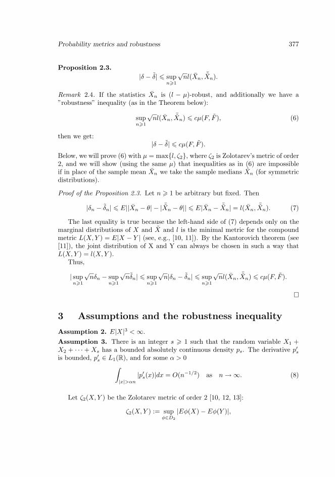
Proposition 2.3.|δ − δ| 6 sup
n>1
√nl(Xn,
¯Xn).
Remark 2.4. If the statistics Xn is (l − µ)-robust, and additionally we have a”robustness” inequality (as in the Theorem below):
supn>1
√nl(Xn,
¯Xn) 6 cµ(F, F ), (6)
then we get:|δ − δ| 6 cµ(F, F ).
Below, we will prove (6) with µ = max{l, ζ2}, where ζ2 is Zolotarev’s metric of order2, and we will show (using the same µ) that inequalities as in (6) are impossibleif in place of the sample mean Xn we take the sample medians Xn (for symmetricdistributions).
Proof of the Proposition 2.3. Let n > 1 be arbitrary but fixed. Then
|δn − δn| 6 E||Xn − θ| − | ¯Xn − θ|| 6 E|Xn − ¯Xn| = l(Xn,¯Xn). (7)
The last equality is true because the left-hand side of (7) depends only on themarginal distributions of X and X and l is the minimal metric for the compoundmetric L(X,Y ) = E|X − Y | (see, e.g., [10, 11]). By the Kantorovich theorem (see[11]), the joint distribution of X and Y can always be chosen in such a way thatL(X,Y ) = l(X,Y ).
Thus,
| supn>1
√nδn − sup
n>1
√nδn| 6 sup
n>1
√n|δn − δn| 6 sup
n>1
√nl(Xn,
¯Xn) 6 cµ(F, F ).
3 Assumptions and the robustness inequality
Assumption 2. E|X|3 <∞.Assumption 3. There is an integer s > 1 such that the random variable X1 +X2 + · · · + Xs has a bounded absolutely continuous density ps. The derivative p′sis bounded, p′s ∈ L1(R), and for some α > 0∫
|x|>αn|p′s(x)|dx = O(n−1/2) as n→∞. (8)
Let ζ2(X,Y ) be the Zolotarev metric of order 2 [10, 12, 13]:
ζ2(X,Y ) := supφ∈D2
|Eφ(X)− Eφ(Y )|,
378 Prague Stochastics 2006
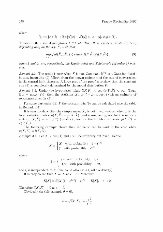
whereD2 := {φ : R → R : |φ′(x)− φ′(y)| 6 |x− y|, x, y ∈ R}.
Theorem 3.1. Let Assumptions 1–3 hold. Then there exists a constant c > 0,depending only on the d.f. F , such that
supn>1
√nl(Xn,
¯Xn) 6 cmax{l(F, F ), ζ2(F, F )}, (9)
where l and ζ2 are, respectively, the Kantorovich and Zolotarev’s (of order 2) met-rics.
Remark 3.2. The result is new when F is non-Gaussian. If F is a Gaussian distri-bution, inequality (9) follows from the known estimates of the rate of convergencein the central limit theorem. A large part of the proof is to show that the constantc in (9) is completely determined by the model distribution F .
Remark 3.3. Under the hypotheses taken l(F, F ) < ∞, ζ2(F, F ) < ∞. Thus,if µ = max{l, ζ2}, then the statistics Xn is (l − µ)-robust (with an estimate ofrobustness given in (9)).
For some particular d.f. F the constant c in (9) can be calculated (see the tablein Remark 4.4).
It is easy to show that the sample mean Xn is not (l− µ)-robust when µ is thetotal variation metric µ(X, X) = σ(X, X) (and consequently, not for the uniformmetric µ(F, F ) = supx |F (x) − F (x)|, nor for the Prokhorov metric µ(F, F ) =π(F, F )).
The following example shows that the same can be said in the case whenµ(X, X) = l(X, X).
Example 3.4. Let X ∼ N(0, 1) and ε > 0 be arbitrary but fixed. Define
X =
{X with probability 1− ε4/3
ξ with probability ε4/3,
where
ξ =
{1/ε with probability 1/2−1/ε with probablity 1/2,
and ξ is independent of X (one could also use a ξ with a density).It is easy to see that X ⇒ X as ε→ 0. Moreover,
E|X| = E|X|(1− ε4/3) + ε1/3 → E|X|, ε→ 0.
Therefore l(X, X) → 0 as ε→ 0.Obviously (in this example θ = 0),
δ =√nE|Xn| =
√2π.

Probability metrics and robustness 379
On the other hand,
Var(X) = σ2(ε) = (1− ε4/3) + ε−2/3 <∞,
and for any fixed ε > 0 √n ¯Xn ⇒ ηε
where ηε ∼ N(0, σ2(ε)). Since the variances of the summands are finite, we have
E|√n ¯Xn| → E|ηε| =
√2πσ(ε), as n→∞.
so that
δ = supn>1
E|√n ¯Xn| >
√2πσ(ε) →∞ as ε→ 0.
So we get l(X, X) → 0, but |δ − δ| → ∞ as ε→ 0.
Now take into account the above Proposition.
4 The proof of the Theorem
Lemma 4.1. Let X,Y, ξ be random variables such that
a) ξ is independent of X and Y;
b) EX = EY ; EX2 <∞, EY 2 <∞;
c) the random variable ξ has a bounded absolutely continuous density fξ such thatf ′ξ ∈ L1(R).
Thenl(X + ξ, Y + ξ) 6 ||f ′ξ||L1ζ2(X,Y ), (10)
where ζ2 is Zolotarev’s metric of order 2.
Proof.
l(X + ξ, Y + ξ) =∫ ∞
−∞dx|∫ ∞
−∞fξ(x− t)[FX(t)− FY (t)]dt|
=∫ ∞
−∞dx|∫ ∞
−∞fξ(x− t)d[
∫ t
−∞[FX(τ)− FY (τ)]dτ ]|. (11)
Since fξ is bounded and EX = EY the integration by parts on the right-handside of (11) yields:
l(X + ξ, Y + ξ) =∫ ∞
−∞dx|∫ ∞
−∞f ′ξ(x− t)[
∫ t
−∞[FX(τ)− FY (τ)]dτ ]dt|

380 Prague Stochastics 2006
6∫ ∞
−∞dx
∫ ∞
−∞|f ′ξ(x− t)||
∫ t
−∞[FX(τ)− FY (τ)]dτ |dt
by Fubini’s theorem
=∫ ∞
−∞dt|∫ t
−∞[FX(τ)− FY (τ)dτ |
∫ ∞
−∞|f ′ξ(x− t)|dx
= ||f ′ξ||L1
∫ ∞
−∞dt|∫ t
−∞[FX(τ)− FY (τ)]dτ |. (12)
The integral term on the right-hand side of (12) is the known (see [10], §14.1)representation of the metric ζ2.
The next lemma is the main part of the proof of Theorem 1. Hopefully it isuseful in a wider context than that of the present paper.
For n = 1, 2, . . . let Sn = X1 + X2 + · · · + Xn; Sn = X1 + X2 + · · · + Xn;σ2 = Var(X) > 0 and EX = EX = θ.
For n > s (see Assumption 3) denote by gn the density of the r.v. Sn/(σ√n).
Lemma 4.2. Under Assumptions 1-3
l(Sn, Sn) 6 cn1/2 max{l(F, F ), ζ2(F, F )}, (13)
wherec = max{(10s− 1)1/2, 5.4d/σ} (14)
andd = sup
n>s
∫ ∞
−∞|g′n(x)|dx <∞. (15)
Remark 4.3. By (4)
l(Sn, Sn) =√nl(
Sn − nθ√n
,Sn − nθ√
n).
For EX2 6= EX2 by the central limit theorem we get that
lim infn→∞
l(Sn − nθ√
n,Sn − nθ√
n) > 0.
Thus, the rate n1/2 on the right-hand side of (13) can not be reduced.Remark 4.4. The constant c in (13), (14) is completely determined by the distribu-tion function F of X. The constant d in (15) can be calculated in some particularcases numerically, using the fact that under our hypotheses∫ ∞
−∞|g′n(x)|dx→
∫ ∞
−∞|( 1√
2πe−x
2/2)′|dx as n→∞.
For, instance we have the following estimates of the constants for normal,gamma, and uniform distributions:

Probability metrics and robustness 381
Distribution d < c <
N(0, σ) 0.798 max{3, 4.31/σ}(s=1)
Γ (2, λ) 1.040 max{3, 3.98/λ}(s=1)
U [0, a] 0.817 max{4.36, 15.29/a}(s=2)
The proof of Lemma 2 uses an improved version of the technique given in [3]and the standard methods of probabilistic metrics in the framework of the centrallimit theorem (see, for instance, [10], [12]).
Making use of the resuts in [4] it is possible to prove a version of inequality (13)for i.i.d. random vectors.
Proof. Let the integer s and α > 0 be from Assumption 3.For n > s we denote by fn and gn the densities of the random variables Sn
and Sn/(σ√n), respectively. First, we show the existence of a finite constant d
(depending on the distribution function F of the r.v. X) such that
supn>s
||g′n|| 6 d, (16)
where (here and in what follows)
||φ|| = ||φ||L1 =∫ ∞
−∞|φ(x)|dx.
We have (n > s)
||g′n|| =∫|x|62
√nα/σ
|g′n(x)|dx+∫|x|>2
√nα/σ
|g′n(x)|dx. (17)
Assumption 3 implies the conditions of Theorem 7 in [9], Ch. VI. Therefore
g′n(x) =1√2π
d2
dx2
[∫ x
−∞e−t
2/2dt− e−x2/2EX
3(x2 − 1)6σ3
√n
]+O(n−1/2) as n→∞,
(18)where the term O(n−1/2) can be chosen independent of x ∈ R.
From (18) it follows that the first summands in (17) are uniformly bounded inn.
For n > s (see Assumption 3):
fn(x) =∫ ∞
−∞ps(x− t)fn−s(t)dt (19)

382 Prague Stochastics 2006
and since p′s is bounded and it belongs to L1(R) we can differentiate under the sighof integral in (19) (almost everywhere on R, see [2], Appendix A)
f ′n(x) =∫ ∞
−∞p′s(x− t)fn−s(t)dt.
Also g′n(x) = σ2nf ′n(σ√nx). Thus (applying Fubini’s theorem),∫
|x|>2√nα/σ
|g′n(x)|dx = σ√n
∫|z|>2αn
dz|∫ ∞
∞p′s(z − t)fn−s(t)dt|
6 σ√n
∫|t|6αn
fn−s(t)dt∫|z|>2αn
|p′s(z − t)|dz
+σ√n
∫|t|>αn
fn−s(t)dt∫|z|>2αn
|p′s(z − t)|dz = I1,n + I2,n.
By (8)
I1,n 6 σ√n
∫|t|6αn
fn−s(t)dt∫|y|>αn
|p′s(y)|dy = O(1). (20)
Also,I2,n 6 σ
√n||p′s||P (|X1 +X2 + · · ·+Xn−s| > αn)
6 σ√n||p′s||
(n− s)σ2
αn2= O(n−1/2). (21)
Finally, from (17), (20), (21) it follows (16).Let us turn now to the proof of inequality (13). Because of the regularity of the
metric l (see, e.g. [11]):l(Sn, Sn) 6 nl(X1, X1).
Thus, inequalities (13) hold for n 6 10s− 1, provided that
c > (10s− 1)1/2. (22)
For n > 10s let m = [9n/10].For independent r.v.’s X,Z,U, V we have ([11], §8.1):
l(X + U,Z + U) 6 l(X,Z)σ(U, V ) + l(Z + V,Z + V ). (23)
Let Sk,n = Xk+1 + · · ·+Xn, Sk,n = Xk+1 + · · ·+ Xn, 0 6 k 6 n.Applying the triangular inequality and (23) to X = Sm,n, Z = Sm,n, U = S0,m,
V = S0,m we getl(Sn, Sn) = l(S0,m + Sm,n, S0,m + Sm,n)
6 l(S0,m + Sm,n, S0,m + Sm,n) + l(S0,m + Sm,n, S0,m + Sm,n)
6 l(S0,m + Sm,n, S0,m + Sm,n) + l(S0,m + Sm,n, S0,m + Sm,n)
Probability metrics and robustness 383
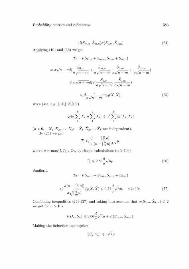
+l(Sm,n, Sm,n)σ(S0,m, S0,m). (24)
Applying (10) and (16) we get
T1 = l(S0,m + Sm,n, S0,m + Sm,n)
= σ√n−ml(
S0,m
σ√n−m
+Sm,n
σ√n−m
,S0,m
σ√n−m
+Sm,n
σ√n−m
)
6 σ√n−mdζ2(
S0,m
σ√n−m
,S0,m
σ√n−m
)
6 d1
σ√n−m
mζ2(X, X), (25)
since (see, e.g. [10],[12],[13])
ζ2(ak∑1
Xi, ak∑1
Xi) 6 a2k∑1
ζ2(Xi, Xi)
(a > 0, X1, X2, . . . , Xk; X1, X2, . . . Xk are independent).By (25) we get
T1 6d
σ
[ 910n]
(n− [ 910n])1/2
µ,
where µ = max{l, ζ2}. Or, by simple calculations (n > 10s)
T1 6 2.85d
σ
√nµ. (26)
Similarly,T2 = l(Sm,n + S0,m, Sm,n + S0,m)
6d(n− [ 9
10n])
σ√
[ 910n]
ζ2(X, X) 6 0.21d
σ
√nµ, n > 10s. (27)
Combining inequalities (24)–(27) and taking into account that σ(S0,m, S0,m) 6 2we get for n > 10s.
l(Dn, Sn) 6 3.06d
σ
√nµ+ 2l(Sm,n, Sm,n).
Making the induction assumption
l(Sk, Sk) 6 c√kµ
384 Prague Stochastics 2006
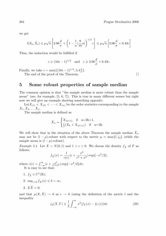
we get
l(Sn, Sn) 6 µ√n
[3.06
d
σ+(
1− 1n
[910n])1/2
c
]6 µ
√n
[3.06
d
σ+ 0.43c
]Thus, the induction would be fulfilled if
c > (10s− 1)1/2 and c > 3.06d
σ+ 0.43c.
Finally, we take c = max{(10s− 1)1/2, 5.4 dσ}.The end of the proof of the Theorem.
5 Some robust properties of sample median
The common opinion is that ”the sample median is more robust than the samplemean” (see, for example, [5, 6, 7]). This is true in many different senses but rightnow we will give an example showing something opposite.
LetX(1) < X(2) < · · · < X(n) be the order statistics corresponding to the sampleX1, X2, . . . Xn.
The sample median is defined as
Xn =
{X(k+1) if n=2k+1,12 (Xk +X(k+1)) if n=2k.
We will show that in the situation of the above Theorem the sample median Xn
may not be (l − µ)-robust with respect to the metric µ = max{l, ζ2} (while thesample mean is (l − µ)-robust).
Example 5.1. Let X ∼ N(0, 1) and 1 > ε > 0. We choose the density fX of F asfollows:
fX(x) =1c(ε)
(ε+x2
ε3 + x2) exp{−x2/2},
where c(ε) =∫∞−∞(ε+ x2
ε3+x2 ) exp{−x2/2}dx.It is easy to see that:
1. fX ∈ C1(R);
2. supε>0 fX(x) 6 b <∞;
3. EX = 0;
and that µ(X, X) → 0 as ε → 0 (using the definition of the metric l and theinequality
ζ2(X,Y ) 612
∫ ∞
−∞x2|fX(x)− fY (x)|dx (28)
Probability metrics and robustness 385
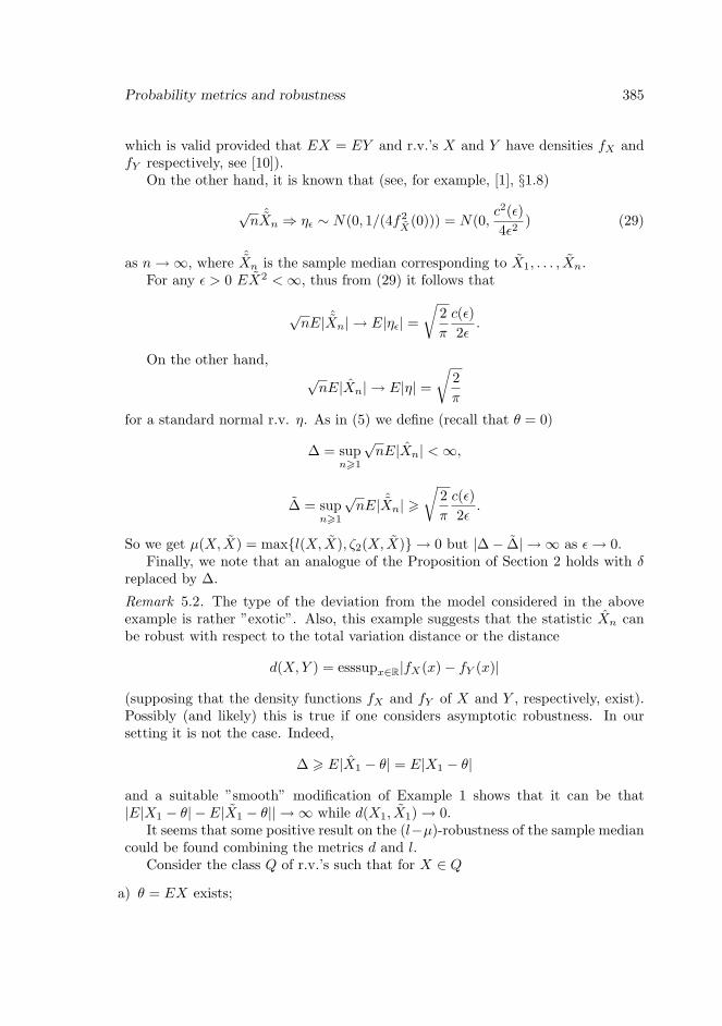
which is valid provided that EX = EY and r.v.’s X and Y have densities fX andfY respectively, see [10]).
On the other hand, it is known that (see, for example, [1], §1.8)
√n ˆXn ⇒ ηε ∼ N(0, 1/(4f2
X(0))) = N(0,
c2(ε)4ε2
) (29)
as n→∞, where ˆXn is the sample median corresponding to X1, . . . , Xn.For any ε > 0 EX2 <∞, thus from (29) it follows that
√nE| ˆXn| → E|ηε| =
√2π
c(ε)2ε
.
On the other hand,√nE|Xn| → E|η| =
√2π
for a standard normal r.v. η. As in (5) we define (recall that θ = 0)
∆ = supn>1
√nE|Xn| <∞,
∆ = supn>1
√nE| ˆXn| >
√2π
c(ε)2ε
.
So we get µ(X, X) = max{l(X, X), ζ2(X, X)} → 0 but |∆− ∆| → ∞ as ε→ 0.Finally, we note that an analogue of the Proposition of Section 2 holds with δ
replaced by ∆.
Remark 5.2. The type of the deviation from the model considered in the aboveexample is rather ”exotic”. Also, this example suggests that the statistic Xn canbe robust with respect to the total variation distance or the distance
d(X,Y ) = esssupx∈R|fX(x)− fY (x)|
(supposing that the density functions fX and fY of X and Y , respectively, exist).Possibly (and likely) this is true if one considers asymptotic robustness. In oursetting it is not the case. Indeed,
∆ > E|X1 − θ| = E|X1 − θ|
and a suitable ”smooth” modification of Example 1 shows that it can be that|E|X1 − θ| − E|X1 − θ|| → ∞ while d(X1, X1) → 0.
It seems that some positive result on the (l−µ)-robustness of the sample mediancould be found combining the metrics d and l.
Consider the class Q of r.v.’s such that for X ∈ Q
a) θ = EX exists;
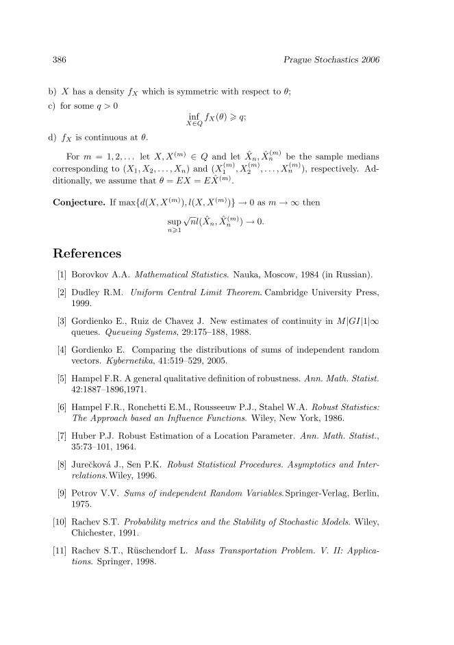
386 Prague Stochastics 2006
b) X has a density fX which is symmetric with respect to θ;
c) for some q > 0infX∈Q
fX(θ) > q;
d) fX is continuous at θ.
For m = 1, 2, . . . let X,X(m) ∈ Q and let Xn, X(m)n be the sample medians
corresponding to (X1, X2, . . . , Xn) and (X(m)1 , X
(m)2 , . . . , X
(m)n ), respectively. Ad-
ditionally, we assume that θ = EX = EX(m).
Conjecture. If max{d(X,X(m)), l(X,X(m))} → 0 as m→∞ then
supn>1
√nl(Xn, X
(m)n ) → 0.
References
[1] Borovkov A.A. Mathematical Statistics. Nauka, Moscow, 1984 (in Russian).
[2] Dudley R.M. Uniform Central Limit Theorem. Cambridge University Press,1999.
[3] Gordienko E., Ruiz de Chavez J. New estimates of continuity in M |GI|1|∞queues. Queueing Systems, 29:175–188, 1988.
[4] Gordienko E. Comparing the distributions of sums of independent randomvectors. Kybernetika, 41:519–529, 2005.
[5] Hampel F.R. A general qualitative definition of robustness. Ann. Math. Statist.42:1887–1896,1971.
[6] Hampel F.R., Ronchetti E.M., Rousseeuw P.J., Stahel W.A. Robust Statistics:The Approach based an Influence Functions. Wiley, New York, 1986.
[7] Huber P.J. Robust Estimation of a Location Parameter. Ann. Math. Statist.,35:73–101, 1964.
[8] Jureckova J., Sen P.K. Robust Statistical Procedures. Asymptotics and Inter-relations.Wiley, 1996.
[9] Petrov V.V. Sums of independent Random Variables. Springer-Verlag, Berlin,1975.
[10] Rachev S.T. Probability metrics and the Stability of Stochastic Models. Wiley,Chichester, 1991.
[11] Rachev S.T., Ruschendorf L. Mass Transportation Problem. V. II: Applica-tions. Springer, 1998.